Transverse Momentum Dependent Gluon Distribution within High Energy Factorization at Next-to-Leading Order
Abstract
We discuss Transverse Momentum Dependent (TMD) gluon distributions within high energy factorization at next-to-leading order in the strong coupling within the framework of Lipatov’s high energy effective action. We provide a detailed discussion of both rapidity divergences related to the TMD definition and its soft factor on the one hand, and rapidity divergences due to high energy factorization on the other hand, and discuss common features and differences between Collins-Soper (CS) and Balitsky-Fadin-Kuarev-Lipatov (BFKL) evolution. While we confirm earlier results which state that the unpolarized and linearly polarized gluon TMD agree in the BFKL limit at leading order, we find that both distributions differ, once next-to-leading order corrections are being included. Unlike previous results, our framework allows to recover the complete anomalous dimension associated with Collins-Soper-Sterman (CSS) evolution of the TMD distribution, including also single-logarithmic terms in the CSS evolution. As an additional result we provide a definition of -factorization, i.e. matching of off-shell coefficients to collinear factorization at next-to-leading order within high energy factorization and the effective action framework. We furthermore establish a link between the QCD operator definition of the TMD gluon distribution and a previously derived off-shell TMD gluon-to-gluon splitting function, which is within the present framework obtained as the real 1-loop correction.
I Introduction
Transverse momentum dependent (TMD) parton distribution functions
(PDFs) [1, 2, 3] are objects of increased
interest, since they allow to provide a more precise kinematic
description of partonic scattering processes already at the leading
order (LO) of perturbation theory. This is in particular true, if the
observable of interest is not entirely inclusive. In that case, TMD
PDFs provide an important advantage over a description based on
collinear parton distributions. TMD PDFs arise naturally in processes
which are characterized by a hierarchy of scales. With the scale of
the hard reactions, TMD PDFs are at first defined for the hierarchy
with the transverse
momentum of the parton and the QCD
characteristic scale of a few hundred MeV. The QCD description of such
events gives then rise to the so-called Collins-Soper-Sterman (CSS)
[4, 5, 6] resummation
formalism. A different kinematic hierarchy in which TMD PDFs arise is
provided by the perturbative Regge or low limit
, where denotes
the center of mass energy of the reaction and . While the
resulting high energy factorization
[7, 8, 9]
does not primarily address the
description of transverse momenta of final states, the ensuing
formalism naturally factorizes cross-sections into transverse momentum dependent coefficients, so
called impact factors, and transverse momentum dependent Green’s function, which summerize logarithms in the center of mass energy. In particular
Balitsky-Fadin-Kuraev-Lipatov
(BFKL) evolution [10, 11, 12, 13, 14, 15], as well as its non-linear extensions,
keep track of transverse momenta along the evolution chain.
Both kinematic limits have a region of overlap, characterized through
the hierarchy , which
is of particular interest due its sensitivity to the emergence of a
semi-hard dynamical scale in the low limit, the so-called
saturation scale [16]. The relation of both
frameworks has been explored in a series of publications
[17, 18, 19, 20, 21, 23, 24, 22, 25] and is currently used for a wide set
of phenomenological studies see e.g.[26, 27, 28, 29, 30, 31]. A somehow
orthogonal approach has been put forward in
[32, 33, 34]:
instead of studying the region of overlap of both kinematic regimes,
the goal has been to derive TMD evolution kernels which are meant to
achieve a simultaneous resummation of both
Dokshitzer-Gribov-Lipatov-Altarelli-Parisi (DGLAP) and BFKL
logarithms [35, 36]. Such an approach seems to be of particular interest for
Monte-Carlo applications such as [37, 38, 39, 40, 41]. While
currently only real splitting kernels have been derived, which reduce
in the regarding limits to the respective real DGLAP and BFKL kernels, the relation to
CSS resummation is at the moment less clear, however the gluon-to-gluon
splitting kernel could be shown to reduce to the
Ciafaloni-Catani-Fiore-Marchesini kernel [42, 43] in the soft limit.
In the following we aim at solving various open questions related to
the previously mentioned studies. In particular we will give a
next-to-leading order (NLO) study with respect to an expansion in the
strong coupling constant of the gluon TMD in the high
energy limit. While a related study has been already presented in
[22] within the Color-Glass-Condensate approach, we
will investigate this problem within the context of Lipatov’s high
energy effective action [44, 45]. Starting
with [46, 47, 48, 49, 50] the systematic determination of
perturbative higher order corrections has been worked out for this
framework, while in [51] equivalence with the
Color-Glass-Condensate formalism has been demonstrated, including an
re-derivation of the Balitsky-JIMWLK evolution, see also
[52, 53] for reviews; for further
recent studies based on this framework see also [54, 55, 56, 57, 58, 59, 60, 61].
In [62] a systematic framework for the
determination of next-to-leading order corrections at cross-section
level has been worked out. For the present study we will further
extend this framework to include asymmetric factorization scale
settings as required for a matching to collinear factorization, i.e. -factorization [8]. While this framework
is currently limited to the dilute regime, i.e. 2 (reggeized)
gluon exchange at the level of the cross-section, it has the great
advantage that it allows to systematically study different choices of
factorization parameter and schemes, which will be of particular use
for the further exploration of the relation between BFKL and Collins-Soper
(CS) [4, 5] evolution, initiated in
[20]. In particular we will determine systematically
the NLO coefficients which relate the QCD operator definition of the
unpolarized and linearly polarized gluon TMD PDF with the unintegrated
gluon density of high energy factorization, which in turn will allow
us to recover the complete CSS resummation scheme in combination with
BFKL evolution, following closely related calculations based on
collinear factorization [63, 64]. We expect our result to be useful for a precise
description of final states with small transverse momenta within high
energy factorized cross-sections, at a similar level of accuracy as
descriptions based on collinear factorization.
Another aspect of our result relates to the derivation of TMD
splitting kernels in
[32, 34]. While the original
derivation was based on a combined implementation of the
Curci-Furmanski-Petronzio formalism for the calculation of the
collinear splitting functions [65] and the framework of
high energy factorization provided by [44], we find
in the following that the real contribution to the QCD operator
definition of the unpolarized gluon TMD yields precisely the
previously derived off-shell TMD splitting kernel. Our current study
provides therefore a possibility to recover the so far missing virtual
corrections to these off-shell splitting kernels.
The outline of this paper is as follows. In Sec. II we
give a precise definition of the goal of this paper in more technical
terms, in particular the definition of the gluon TMD PDFs, Sec. III contains a brief review of Lipatov’s high
energy effective action and presents among other details an extension
of the framework of [62] to
-factorization. In Sec. IV we present the results
of our NLO calculation, while Sec. V discusses
aspects related to the interplay of CS and BFKL evolution. In
Sec. VI we summarize our result and provide an outlook on
future research.
II The setup of our study
The starting point of our study is the TMD factorization of a suitable perturbative process. To be specific we will refer in the following to the transverse momentum distribution of a Higgs boson, as discussed for instance in [64], see also [63]. With and transverse momentum and mass of the Higgs boson, this factorization is valid for and reads:
| (1) |
where is the rapidity of the Higgs boson while denote the hadron momentum fractions of gluons stemming from hadron respectively and
| (2) |
where denotes the rapidity which divides soft gluons from hadron and ; is the renormalization point of the cross-section. To be specific we consider scattering of two hadrons with light-like momenta and which serve to define the light-cone directions
| (3) |
which yields the following Sudakov decomposition of a generic four-momentum,
| (4) |
and . Here, is the embedding of the Euclidean vector into Minkowski space, so . For Eq. (II), the top quark is considered to be integrated out and is the corresponding Wilson coefficient; is the square of the on-shell gluon form factor at time-like momentum transfer , with infrared divergences subtracted, see [66]. To leading order in perturbation theory they equal one, while the precise NLO expression are not of interest for the following discussion and can be found for instance in [64]. is finally the collinear Born level cross-section for the process ,
| (5) |
with GeV the Higgs vacuum expectation value; denotes finally the strong coupling constant at the renormalization point . For an unpolarized hadron, the TMD correlator , can be further decomposed [67]
| (6) |
where denotes the unpolarized TMD gluon distriubtion and the linearly polarized TMD gluon distribution in an unpolarized hadron. In terms of QCD fields the TMD PDF is defined as [63, 64]
| (7) |
where denotes the soft factor and , with a suitable regulator whose precise implementation will be given in Eq. (III.4) below. Gauge links are in general given as a combination of a longitudinal and a transverse gauge link [2], where the transverse gauge link is placed at light-cone infinity. Working in covariant gauge, the gauge field at infinity vanishes and the transverse gauge link therefore equals one. We will therefore in the following not consider the transverse gauge link. The longitudinal gauge link is on the other hand given by
| (8) |
where denotes the gluonic field and
| (9) |
For the soft factor there exists various prescriptions in the literature, see e.g. [68, 63, 64, 2, 69, 70]. To keep the discussion as general as possible, we will consider below the most general soft factor introduced in [2, 69],
| (10) |
with
| (11) |
where are tilted Wilson lines such that is
placed at rapidity111Due to the regulator defined in
Sec. III.4 this implies in our case also an
imaginary part; the above expressions refer to the corresponding
real parts, while imaginary parts cancel for the final result
and at rapidity . For a precise definition of
the light-cone directions see Eq. (III.4) further below. The
goal of the following sections is to study this gluon TMD in the high
energy limit at next-to-leading order. In particular we will discuss
the factorization of this TMD PDF into a perturbative coefficient, the
BFKL gluon Green’s function, and a hadronic impact factor. The latter
two will then form the so-called unintegrated gluon density within
high energy factorization. Our study is limited to the exchange of 2
reggeized gluons. It is known from various studies, that the gluon TMD
also receives corrections due to the exchange of multiple reggeized
gluons, which are of importance to take into account corrections due
to high gluon densities and their possible saturation, see e.g.
[17, 71, 24, 29, 27]. While these are very
interesting questions – in particular since they can provide
modifications of the region of very small transverse momenta due to
the emergence of a saturation scale – we do not consider these
effects in the following. Instead, great care will be taken to provide
a complete discussion of various factorization scales and parameters
both due to factorization in the soft-limit and the high energy limit,
as well as UV renormalization. The study of these effects is somehow
more straightforward, if the observable is restricted to 2 reggeized gluon
exchange, which is the reason why we focus on this limit in the
following. The obtained results may then be generalized at a later
stage to the case of multiple reggeized gluon exchange.
Another motivation for this study is to link the above gluon TMD to the TMD splitting kernels derived in [32, 34]. Below we will demonstrate that the TMD gluon-to-gluon splitting of [34] arises directly from the real contributions to the 1-loop coefficient. We believe that this is a very interesting result, since it allows us to connect the framework of real TMD splitting kernels to the above operator definitions of TMD PDFs.
III The High-Energy Effective Action
Since the current study requires a small but important generalization in comparison to the framework presented in [29], we begin our study with a short review of the high energy effective action and the resulting calculational framework for NLO calculations. Our treatment of high energy factorization is based on Lipatov’s high energy effective action [44]. Within this framework, QCD amplitudes are in the high energy limit decomposed into gauge invariant sub-amplitudes which are localized in rapidity space and describe the coupling of quarks (), gluon () and ghost () fields to a new degree of freedom, the reggeized gluon field . The latter is introduced as a convenient tool to reconstruct the complete QCD amplitudes in the high energy limit out of the sub-amplitudes restricted to small rapidity intervals. Lipatov’s effective action is then obtained by adding an induced term to the QCD action ,
| (12) |
where the induced term describes the coupling of the gluonic field to the reggeized gluon field . High energy factorized amplitudes reveal strong ordering in plus and minus components of momenta which is reflected in the following kinematic constraint obeyed by the reggeized gluon field:
| (13) |
Even though the reggeized gluon field is charged under the QCD gauge group SU, it is invariant under local gauge transformation . Its kinetic term and the gauge invariant coupling to the QCD gluon field are contained in the induced term
| (14) |
with
| (15) |
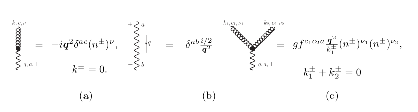
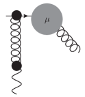
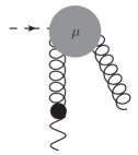
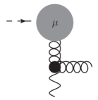
For a more in depth discussion of the effective action we refer to the reviews [52, 53]. Due to the induced term in Eq. (12), the Feynman rules of the effective action comprise, apart from the usual QCD Feynman rules, the propagator of the reggeized gluon and an infinite number of so-called induced vertices. Vertices and propagators needed for the current study are collected in Fig. 1. Determination of NLO corrections using this effective action approach has been addressed recently in series of publications [46, 48, 49, 50, 47]. For a discussion of the analogous high energy effective for flavor exchange [72] at NLO see e.g. [73, 74, 75].
III.1 Determination of NLO coefficients


The framework for the determination of NLO corrections has been established in [62] within the determination of the NLO forward Higgs production coefficient in the infinite top mass limit. We will therefore frequently refer to process
| (16) |
as an example process in the following, where we further assume that the particles in the fragmentation region of the scattering particles are widely separated in rapidity. The partonic impact factor of the quark with momentum will be later on replaced by the hadronic impact factor, which forms together with the BFKL Green’s function the unintegrated gluon density. As in [62], we will consider matrix elements normalized to match corresponding collinear matrix elements for vanishing virtuality of the reggeized gluon state. We therefore have
| (17) |
where we average over incoming parton color as well as the color of the reggeized gluon and sum over the color of produced particles; denotes the -particle system produced in the regarding fragmentation region. With
| (18) |
we arrive at the following definition of an off-shell partonic cross-section and the corresponding impact factor :
| (19) |
Note that this impact factor can in principle be arbitrarily differential, as far as the formulation of high energy factorization is concerned; for a corresponding definition of the other impact factor we refer to [62]. The above expression is subject to so-called rapidity divergences which are understood to be regulated through lower cut-offs on the rapidity of all particles, with and for the number of particles produced in the fragmentation region of the initial parton . For virtual corrections, the regularization is achieved through tilting light-cone directions of the high energy effective action,
| (20) |
Below we will also comment on the possibility to regularize rapidity
divergences through tilting light-cone direction also in the case of
real corrections, see Sec. III.4.
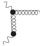
As shown through explicit results [46, 48, 49, 50, 62], impact factors contain beyond leading order configurations, which reproduce factorized contributions with internal reggeized gluon exchange. It is therefore necessary to subtract these contributions, see also Fig. 2. To this end one defines the bare one-loop 2-reggeized-gluon Green’s function as well as the impact factors through the following perturbative expansion
| (21) |
Using the following convolution convention
| (22) |
we then define the following subtracted bare NLO coefficient,
| (23) |
and 222Note that the impact factors themselves might depend on additional transverse momenta; this is however irrelevant for the following discussion of high energy factorization and we therefore suppress this dependence in the following.
| (24) |
where we added the super-scripts ‘’ and ‘’ to indicate that the impact factor of the particle with momentum refers to the hard event and the unintegrated gluon distribution respectively. While rapidity divergences cancel for the the above expression, its elements still depend on the regulator. As a next step we therefore define a renormalized Green’s function through
| (25) |
which yields
| (26) |
where
| (27) |
The transition functions have a twofold purpose: they both serve to cancel -dependent terms between impact factors and Green’s function and allow to define the BFKL kernel. In particular,
| (28) |
where
| (29) |
III.2 Transition function and finite terms
In the following we generalize the treatment given in [62] through including as well the most general finite contribution into our discussion. The need to include finite contribution into this transition factors has been first realized in the determination of the 2-loop gluon Regge trajectory in [50, 49, 48], where both divergent and finite terms could be simply taken to exponentiate, since one is dealing with 1-reggeized gluon exchange contributions only. A suitable generalization, which both reduces to the exponential ansatz of [50] and obeys Eq. (III.1), is then given by
| (30) |
which is sufficient for a discussion up to NLO accuracy. As we will see in the following, these finite contributions serve a twofold purpose. At first they remove a potential finite contribution in the bare Green’s function,
| (31) |
where
| (32) |
which then yields directly the 1-loop BFKL kernel
| (33) |
To keep the treatment as general as possible, the finite contribution is on the other hand then split up into 2 terms:
| (34) |
The contribution is used to transfer finite terms contained in the Green’s function to the impact factors. We take in the following this function to be identical for both plus and minus direction . Indeed, since we are essentially dealing with contributions due to the gluon polarization tensor in the high energy limit, such a symmetric treatment appears to be the appropriate one. One finds
| (35) |
The second contribution was absent in the discussion of [62]. It needs to satisfy to 1-loop the following requirement, to ensure absence of finite terms in the Green’s function:
| (36) |
Note that similar constraints can be imposed on higher order contributions to the functions to achieve a Green’s function without finite contributions at higher orders. Including all contributions, one finally arrives at following expression for the NLO coefficient:
| (37) |
where and are given in Eq. (III.2) and Eq. (III.2) respectively. The function as well as the evolution parameters are on the other hand still undetermined. They are in principle arbitrary, but should be chosen such that both impact factors are free of large logarithms.
III.3 Scale setting for -factorization
The parameters as well as the function are at first arbitrary; the former define through the combination the evolution parameter of the 2 reggeized gluon Green’s function , see also the related discussion in [62, 53]. As usually, it is necessary to chose these parameters such that the next-to-leading order corrections to impact factors are under perturbative control and that large logarithms in the center of mass energy are resumed through the 2 reggeized gluon Green’s function. Within the -factorization setup, one of the impact factors, e.g. the coefficient in our example, is to be replaced by the hadronic impact factor, which then builds together with the BFKL Green’s function the unintegrated gluon density. Even though the hadronic impact factor is naturally a non-perturbative object, at the very least for transverse momenta GeV, it must have an expansion in terms of collinear parton distribution functions and corresponding collinear coefficients, see e.g. [76]. In order to have a complete matching of the resulting expression for the unintegrated gluon density to the collinear gluon distribution in the double-logarithmic limit, it is natural to chose the evolution parameter to coincide with the fraction of the hadronic momentum carried on by the gluon with the invariant mass of the system produced in the fragmentation region333This relation is exact for the scattering of a parton with a hadron . Note that at NLO, an asymmetric scale choice, i.e. choosing the reference scale of the center-of-mass energy to be of the order of a typical scale of one of the impact factors, leads to a modification of the NLO BFKL kernel, see e.g. [14, 77]. To repeat this exercise within the context of the high energy effective action, we reconsider Eq. (III.1), but focuse now on the factorization parameters and the finite terms introduced above:
| (38) |
where is the invariant mass of the produced final state corresponding to each of the impact factors and collects all terms which are independent of both and . To equal the evolution parameter of the Green’s function with the hadron momentum fraction carried on by the reggeized gluon entering the impact factor , we set
| (39) |
where are so far unspecified reference scale and is a parameter of order one, which allows to estimate the scale uncertainty associated with high energy factorization. In the following we chose to be of the order of , i.e. the hard scale. While this is a natural choice for the hard impact factor, it introduces the same scale into the hadronic impact factor, characterized in general by small transverse momenta. We therefore find in the perturbative region of the hadronic impact factor a large collinear logarithm, which at first spoils the convergence of the perturbative expansion. This logarithm can however be absorbed into the function through setting
| (40) |
which eliminates the logarithm in from the hadronic impact factor. Note that the choice of as the relative scale is somewhat arbitary, and other choices are equally possible, see e.g. [76]. It is interesting to compare this situation to the case where the parameters are identified with the rapidities of the system produced in the regarding fragmentation region, , , with . One finds
| (41) |
which allows to verify that the presented treatment agrees – after setting – with the one derived in [77], based on a study of ladder diagrams within the Quasi-Multi-Regge-Kinematics in the context of the definition of the NLO inclusive jet vertex. For the NLO BFKL kernel one finally obtains the following contribution
| (42) |
which is independent of the parameter and where denotes the NLO BFKL kernel if is identified with the rapidities of the external particles with . The above expression is in agreement with [77] and [14]. A more detailed discussion of possible choices of the function will be presented elsewhere.
Summing up we have the general definition of the unintegrated gluon density
| (43) |
where we suppressed the dependence on the invariant mass since the latter can in general be expressed in terms of the transverse momentum. The -factorization scheme fixes then through Eq. (40), while is set to . The high energy factorized cross-section is then obtained as
| (44) |
where ‘’might either denote a parton , a partonic impact factor convoluted with a parton distribution function of a hadron or a colorless initial state which allows for a perturbative treatment. Concluding we remark that in [78] a definition of the unintegrated gluon density has been proposed in terms of a operator definition with the high energy gluonic field in light-cone gauge, which requires the inclusion of both so-called 2,3, and 4 body contributions. While an interpretation of such contributions in terms of induced vertices Fig. 1 of the high energy effective action appears to be possible, the precise relation remains unclear.
III.4 Regularization of rapidity divergences


As pointed out in the above discussion, high energy factorized matrix
elements are subject to so-called rapidity divergences. While they
cancel at the level of observables after subtraction of factorizing
contribution and use of the transition function, intermediate results
beyond leading order require a regulator in order to arrive at
well-defined matrix elements. While for real production a cut-off on
the rapidity of produced particles provides a natural way to regulate
such divergences, a consistent regularization is more difficult to
achieve in the case of virtual diagrams. As already pointed out in
Sec. III.1, a suitable way to regulate these
divergences in the case of virtual corrections is to tilt the
light-cone directions of the high energy effective action away from
the light-cone, see Eq. (20). Note that from a formal point of view this a very attractive way of
regularizing rapidity divergences, since gauge invariance of the high
energy effective action does not depend on the property
; tilting light cone directions provides therefore a
gauge invariant regulator, similar to dimensional
regularization. Nevertheless the current treatment, see e.g.
[46, 48, 62] is
somewhat unsatisfactory, since it treats real (cut-off) and virtual
(tilting) corrections on somewhat different grounds. At the same time,
tilting light-cone directions is also a frequently used regulator for
the determination of the 1-loop corrections to TMD PDFs within
collinear factorization, see e.g. [63, 2] and references therein, which is being use for both
real and virtual corrections. It seems therefore natural to regulate
rapidity divergences through tilting light-cone directions also in the
case of real corrections.
From a technical point, this does not imply any major complications. However the real part of the 1-loop Green’s function Eq. (III.2) would receive a finite correction which in covariant Feynman gauge is related to the square of the induced diagrams (last 2 diagrams in Fig. 3). As can be seen already at the level of diagrams, such contributions arise as well for the corresponding impact factors, which contain an identical diagram once calculating the correction due to the emission of an additional real gluon. As a consequence, it is straightforward to show that the corresponding contributions cancel, once subtracted impact factor and central contribution are being combined. Moreover, such a contribution may be easily absorbed into a generalized version of the function , Eq. (III.2). While including such contributions does not provide any substantial complication, one deals in that case with an entirely spurious contribution, which merely arises due to our choice of our regulator and which has no physical meaning. It seems therefore natural to employ a regulator which avoids such a contribution altogether, at least at 1-loop. The modified regulator is essentially identical to the previously used tilted light-cone vectors, while the tilted elements are taken now to be complex, i.e. we will use in the following
| (45) |
As a consequence one has for virtual corrections
| (46) |
while real corrections yields
| (47) |
The spurious self-energy like contributions are therefore absent. The only disadvantage of this method is that terms of the form in virtual corrections can give rise to undesired imaginary parts due to space-like . While at cross-section level such imaginary parts cancel naturally, if one limits oneself to NLO corrections, a consistent treatment of such contribution at amplitude level would require to absorb this imaginary part into the parameter , e.g. through a suitable replacement etc. in the transition functions.
In the following calculation we will meet rapidity divergences which originate both from high energy factorization and the QCD operator definition of the TMD gluon distribution and the corresponding soft factor, which we will consistently regulate through the tilting as described in Eq. (45), while we reserve the use of the regulator for rapidity divergences due to high energy factorization. To be specific we define in the following the tilted Wilson lines of the TMD definition Eq. (II) and Eq. (II) as
| (48) |
IV Determination of the gluon TMD
The goal of the following section is to determine the gluon TMD Eq. (II) within high energy factorization, i.e. we aim at the determination of the following coefficient , implicitly defined through
| (49) |
Note that the TMD PDFs at first do not depend on the proton momentum fraction , since high energy factorization requires to integrate over this longitudinal momentum fraction. Such a dependence therefore only arises through a special choice for the parameters . To allow for a separate discussion of the different contributions of the gluon TMD, we further define
| (50) |
where for the moment we define the TMD PDF in dimensions, since individual expressions are divergent and . We therefore obtain
| (51) |
In the following we evaluate the above gluon TMD for an initial reggeized gluon state with polarization at 1-loop. To be precise we consider
| (52) |
where the reggeized gluon state is defined with the normalization Eq. (17), appropriate for matching to collinear factorization in the limit of vanishing transverse momentum,i.e.
| (53) |
while high energy factorization requires to integrate over the minus momentum,
| (54) |
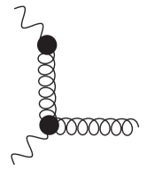
Feynman rules for the determination of perturbative corrections are summarized in Fig. 4. With the following convention to denote the perturbative expansion in for a generic quantity
| (55) |
where , we have finally at leading order
| (56) |
and therefore
| (57) |
and the TMD gluon distributions are up to an overall factor444The overall factor arises since – at least at the level of bare distributions – the unintegrated gluon density reduces to the collinear gluon in the double logarithmic limit after integration over while the gluon TMD requires an integral over , which gives rise to a relative factor of . of at leading order identical to the unintegrated gluon density [17]
| (58) |
where the -factorization scheme defined in Sec. III.3 yields expression which are closest to conventional collinear factorization results. Note that the unintegrated gluon density is therefore directly related to the operator definition of the gluon TMD. Moreover, in the dilute limit i.e. considering only 2 reggeized gluon exchange, the unintegrated gluon density is universal555Note that this universality breaks down, once corrections due to multiple reggeized gluon exchange are included see e.g. [24]. We further stress that the distribution of linearly polarized gluons in an unpolarized hadron is non-zero within high energy factorization already at tree level, in contrast to the result found within collinear factorization [64]. From a technical point of view this is of course easily understood, since the initial gluon carries within high energy factorization already finite and therefore gives rise to such a distribution.
IV.1 One-loop calculation without soft-factor
To regularize infrared and ultraviolet divergences we use dimensional regularization in . The virtual 1-loop correction is provided by the set of diagrams Fig. LABEL:fig:virtual2. The last diagram in the second line vanish within dimensional regularization, since it is scale-less. Including the contribution from the complex conjugate amplitude, we obtain the following result
| (59) |
To obtain the projections on the distribution for the unpolarized TMD PDF and the linearly polarized gluons in an unpolarized hadron, we use
| (60) |
which amounts to replace the overall tensor structure by one for both the unpolarized and the linearly polarized TMD. In particular, due to the presence of non-zero initial transverse momentum, the virtual correction for both TMD distributions are non-zero and agree with each other. Diagrams for real corrections are depicted in Fig. 6. Parameterizing and correspondingly , a straightforward calculation yields
| (61) |
where
| (62) |
where we kept only track of those contributions of order and which are needed to regulate integrals over the momentum fraction and/or transverse momenta, which are not convergent within dimensional regularization. Real splitting functions for the unpolarized () and linearly polarized () gluon read
| (63) | ||||
| (64) |
where we used . Note that the splitting function corresponding to coincides with the real transverse momentum splitting function derived in [34] if we set .


As demonstrated in [34], this splitting function coincides with the DGLAP splitting function in the limit , reduces to the real part of the leading order BFKL kernel in the limit and yields the real leading order kernel of the CCFM equation in the limit . The present calculation provides on the other hand an opportunity to determine the still missing virtual contribution to this splitting function. We further note – in agreement with the result presented in [64] – that the coefficient of the singularity vanishes for the polarized splitting, Eq. (IV.1) in the collinear limit , after averaging additionally over the azimuthal angle of the incoming gluon. For finite this singularity is on the other hand present and requires a treatment similar to the case of the unpolarized gluon TMD PDF. With the integrated real corrections – relevant for the current discussion which is based on high energy factorization – we finally have:
| (65) |
with
| (66) | ||||
| (67) |
where the remaining integrals over are finite and is defined in Eq. (32). If inserted into Eq. (IV), the convolution integral over the reggeized gluon momentum gives still rise to an infra-red singularity. A possibility to extract these singularities is the use of a phase space slicing parameter, see e.g. [81, 80, 79] for an example within the high energy effective action. While this is sufficient to demonstrate finiteness at a formal level, the use of such phase space slicing parameters is in general complicated for numerical studies at NLO accuracy. For the case of collinear NLO calculation, the by now conventional tool to overcome this difficulty are subtraction methods, in particular dipole subtraction [82]. In [62] this has been slightly generalized and applied to the case of divergences which arise due to convolution integrals of transverse momenta. In particular the following decomposition has been proposed:
| (68) |
with
| (69) |
The expression in the squared brackets on the right-hand side vanish in the limit , and is a function which parameterizes the transverse momentum dependence of the reggeized gluon state. The function is such that the integral on the right hand side of (IV.1) is well-defined, which in practice means that it does not behave worse than for and . Furthermore, it should be such that the integral in the second line of (IV.1) can be calculated analytically. Note that the factor is needed to achieve convergence in the ultraviolet. In the current setup we merely require the case with
| (70) |
and
| (71) | ||||
| (72) |
where the corresponding convolution integral can now be defined in dimensions.
IV.2 Soft factor, counter terms and renormalization
The above result contains both rapidity divergences due to high energy factorization and the TMD definition () as well as single and double poles in . Rapidity divergences due to high energy factorization require the subtraction of high energy factorized contributions to the above correlator as well as the application of the transition function, as given by Eq. (III.2). Rapidity divergences due to soft radiation require the soft factor Eq. (10) which we did not include so far. With the 1-loop expansion
| (73) |
and taking the limit666See [69] and [70] for a detailed discussion of these limits , we obtain finally for the soft function in momentum space at 1-loop
| (74) |
where is a finite rapidity and takes a role related to a factorization scale, similar to the parameter in the case of high energy factorization; in particular it enters directly the defintion of the scales defined in Eq. (2). The 1-loop contribution to the TMD gluon densities due to the soft function is finally given by
| (75) |
Note that the 1-loop soft-function, which consists of its real part only within dimensional regularization, agrees with the real part of the 1-loop BFKL kernel. We believe that this coincidence is limited to the 1-loop case and does not hint at a general universality of the rapidity dependence of the soft function. In particular, at the diagrammatic level the soft-function does not give rise to the complete Lipatov vertex, but only to terms related to the induced contributions, see also the discussion in [83] in the context of soft-collinear effective theory for high energy scattering.
As a last step we need to combine virtual (Eq. (IV.1) and real (Eqs. (66)(IV.1)) corrections, with the soft factor, making use of the appropriate projections. Note that the contribution of the soft-factor merely amounts to a replacement of the regulator by the factorization parameter . We obtain for the 1-loop high energy subtracted and renormalized 1-loop coefficients the following result:
| (76) | ||||
| (77) |
where
| (78) |
While the above expression no longer carries rapidity divergences, it still comes with several poles in , which are of ultraviolet origin and which require renormalization. The corresponding renormalization constant is identical for both unpolarized and linearly polarized gluons and is obtained as
| (79) |
which gives rise to the following anomalous dimension
| (80) |
where we used and . Note that the above anomalous dimension agrees with the corresponding result obtained within a treatment based on collinear factorization [64]. This is indeed to be expected since it arises due to the renormalization of ultraviolet divergences, which are naturally independent of the non-zero transverse momentum of the initial state gluon. We however stress that the linearly polarized TMD gluon distribution does not give rise to the above anomalous dimension within collinear factorization, since the corresponding distribution vanishes within collinear factorization at tree-level; the 1-loop result is therefore not renormalized. We finally obtained for the renormalized coefficients
| (81) | ||||
| (82) |
where we made now the dependence on various parameters and explicit. The above expressions for the 1-loop cofficients of unpolarized and linearly polarized gluon TMD are one of the main results of this work.
V Evolution
The coefficients Eqs. (IV.2), (IV.2) depend on three factorization scales and/or parameters: (renormalization scale), (evolution parameter of the soft function) and (evolution parameter of the unintegrated gluon density). In addition we still have the dependence on the function , which is also related to the unintegrated gluon density. The dependence on the renormalization scale and the factorization parameter gives rise to CSS resummation framework, [4, 5, 6]. In the treatment established for collinear initial states, see e.g. [2, 64, 84] it is customary to consider to this end the Fourier-transform of the TMD coefficient to transverse coordinate space
| (83) |
where and then to evolve the coefficient in coordinate space,
| (84) |
with the evolution operator
| (85) |
In the above expression, the CS kernel is in general assumed to have both perturbative and non-perturbative contributions; for a detailed discussion see [2, 64, 84]. The non-perturbative contribution arises due to the inverse Fourier transform, which requires to integrate over large values of , well into the non-perturbative region. Note that a similar statement applies in principle for the convolution integral of Eq. (V.2), if the unintegrated gluon distribution does not drop-off sufficiently fast for small values of transverse momentum . The actual evolution takes place in two steps: first one evolves the coefficient at a certain initial renormalization scale from an initial rapidity – parameterized through , – to a final rapidity . The second step evolves then the TMD PDF from the initial to the final renormalization scale. While the value of the final renormalization scale is of the order of the hard scale, i.e. the Higgs mass for the current example, the initial renormalization scale must be chosen such that it minimizes the perturbative correction to the TMD coefficients. In collinear calculations it it is naturally taken to be of the order of the transverse momentum or its inverse conjugate coordinate with the Euler constant. In the current setup, the optimal choice is far from apparent, since the coefficients depend on multiple scales due to non-zero initial transverse momenta. In particular, the transverse momenta and are at least at first not necessarily of the same order of magnitude.
V.1 A comparison of the kernels of CS and BFKL evolution
Both CS and BFKL evolution describe evolution in rapidity. It is therefore natural to expect that both evolution and their respective kernels have a certain overlap. For the derivation of the CS kernel, we follow closely [2, 84], where the kernel of the Collins-Soper evolution equation is defined through the dependence of the renormalized soft factor,
| (86) |
and is itself subject to the following renormalization group equation,
| (87) |
where is the cusp anomalous dimension in the adjoint representation, see [85, 86, 64] for higher order terms. At 1-loop one finds
| (88) |
While the representation in transverse coordinate space is very useful for a direct solution of the CS-equation through exponentiation of the CS kernel as in Eq. (V), it is also instructive to formulate the CS-equation in momentum space, which allows for a direct comparison with the BFKL equation. In particular, defining in complete analogy to the BFKL treatment a CS Green’s function , BFKL, CS, such that
| (89) |
one finds at 1-loop the following simple relation between both kernels:
| (90) |
The presence of this factor can be explained as follows. As it is well known, the virtual correction to the 1-loop BFKL kernel is directly related to the gluon Regge trajectory which in transverse momentum space can be written as
| (91) |
The CS equation is on the other hand limited to soft radiation, which implies restriction to transverse momenta and . The integrand in the above expression therefore reduces to
| (92) |
and the integral vanishes within dimensional regularization through a cancellation of the infra-red and ultra-violet poles. Removing on the other hand the UV pole through renormalization, one finally ends up with the virtual contribution to the CS kernel. The CS evolution can be therefore understood as the soft approximation to the complete BFKL kernel. Indeed, such an identification is natural, since the CS kernel arises from the rapidity divergence of the soft-function, while the BFKL kernel from the rapidity divergence of partonic cross-sections in the high energy limit .
The above discussion clearly suggests that the CS and BFKL evolution are closely related to each other, with the CS kernel as the soft limit of the complete BFKL kernel. When considering CS and BFKL evolution for the same quantity, it is therefore necessary to remove the overlap of both evolution equations or alternatively to restrict them to distinct regions in phase space, which are then covered by the regarding evolution equation. In particular the various evolution parameters must obey the following ordering
| (93) |
it is needed to separate the phase space covered by BFKL evolution (rapidity evolution of the entire cross-section) and CS evolution (rapidity evolution of soft gluons only). Clearly, soft gluons form a sub-set of the complete cross-section and cannot be evolved separately from the latter in rapidity.
V.2 factorization and alternative schemes
In the following we investigate our result for a specific choice of the evolution parameter of the unintegrated gluon density ,which we fix to coincide with the proton momentum fraction , i.e. we consider now the equivalent of Eq. (IV), but with the following choices for the parameters of the high energy evolution, following the results of Sec. III.3
| (94) |
where is a still unspecified reference scale. The coefficients take the following form
| (95) | ||||
| (96) |
with . Even though both and the function depend within this scheme on a certain reference scale , the dependence on this scale cancels between both contributions, and we remain only with the parameter which is of order one. The scale remains therefore unspecified and can be used to satisfy the ordering condition Eq. (93). A possible and suitable choice is then , with another constant of order one, which eliminates a potential large logarithm in the coefficients and which specifies eventually . The complete resummed gluon TMDs take then the following final form
| (97) |
where and are yet unspecified scales. Reading the above expressions from the right to the left, one first evolves the unintegrated gluon density through BFKL evolution up to the hadron momentum fraction , with a corresponding factorization uncertainty parametrized through . The unintegrated gluon distribution is then convoluted with the NLO TMD coefficient in transverse momentum . The resulting expression defines then the gluon TMD with transverse momentum at a scale and renormalization point . While is an arbitary scale, introduced to define the -factorization scheme, it is naturally chosen to be of the order of the transverse momentum ; the same is true for the choice of the renormalization point . In a next step it is therefore needed to evolve this gluon TMD both in (rapidity evolution of soft gluons) and finally in the renormalization scale to its final values, where rapidity evolution of solution gives rise to a convolution in transverse momentum . The above expressions for CSS evolution (combined evolution in and ) are the conventional expresses found in the literature, while they are expressed in transverse momentum instead of transverse coordinate space. In particular, the CS Green’s function in transverse momentum space is obtained from the frequently used transverse coordinate expression through
| (98) |
At 1-loop, is given by Eq. (86). For perturbative higher orders see e.g. Sec. III of [64], where it is needed to include a relative factor of 2 with respect to the convention employed in this paper. Apart from perturbative higher order corrections, one might also consider RG evolution from the scale to a suitable renormalization point of the CS Green’s function; finally it is also possible to include a model for non-perturbative effects. If one restricts oneself on the other hand to the leading order kernel Eq. (86), the above integral can be easily evaluated and one finds
| (99) |
with . Note that convergence of the Fourier integral requires for the above expression. While the kernels of CSS and BFKL evolution in Eq. (V.2) are well known, our result provides as a new element the perturbative coefficient which connects both evolution equations up to NLO accuracy. In particular, a complete next-to-leading logaritmic resummation of both BFKL and CSS logarithms requires to combine the NLO coefficient Eqs. (V.2), (V.2) with the unintegratd gluon distribution evolved with the NLO BFKL kernel [14] as well as CSS evolution with NLO anomalous dimension Eq. (IV.2), and the corresponding expression for the CS kernel, see [64] for a compact summary up to NNLO accuracy of these elements in the gluonic channel. It would be very interesting to compare this result to the low expansion of exact N3LO results for the gluon TMD PDFs [87]. From a technical point of view, this would require to construct a partonic unintegrated gluon distribtion, following Eq. (III.3), but using NLO quark and gluon impact factors.
While the identification of the evolution parameter according to the -scheme, as used above, provides a direct generalization of the collinear result and is been often employed in fits of the unintegrated gluon density, see e.g. [88, 89, 90, 91], it is not necessarily the most adequate to describe rapidity evolution of the system. An alternative form would be to identify with the maximal rapidity of the soft gluonic system, or with the rapidity of the hard final state, i.e. the Higgs boson . While eliminates entirely the need for CS evolution, it also ignores the rapidity of the hard event (Higgs boson) in the energy evolution of the TMD PDF. The choice appears therefore to be possilbe, but inadequate. The choice evolves the unintegrated gluon density through BFKL evolution up to the rapidity of the hard even, while CS evolution addresses the possible differences , where both and is possible. Introducing furthermore the parameter , which allows to address the scale uncertainty associated with high energy factorization, i.e. high energy evolution describes dependence on and is taken to be of order one, one finds
| (100) |
where , and is a parameter of the order of the hadron rapidity. Note that within this frame, the TMD PDFs no longer depend on the hadron momentum fraction, but rather on rapidity. While this might appear strange at first sight, it is natural from the point of view of high energy factorization where the momentum fraction is – in the case of the -factorization scheme – merely an evolution parameter fixed through the kinematics of the final state, while the above rapidity scheme uses a different choice for this evolution parameter.
V.3 Relation to previous results in the literature
Before we conclude, we briefly discuss the relation of the above
results to results in the literature. In principle the TMD gluon
distribution has been already study within high energy factorization
at NLO in [22], previous studies with a similar scope
are [20] and [92, 93]. At
the level of real corrections, the contributions seem to be identical
at the level of Feynman diagrams, leaving aside the absence of the
multiple reggeized gluon exchange in the current discussion. The set
of virtual diagrams of [22] is on the other hand
clearly reduced with respect to the ones considered in this work,
Fig. LABEL:fig:virtual2. Indeed, the authors of [22]
seem to consider only self-energy corrections to the Wilson line in their
approach. This difference is direcly related to the fact that
[22] makes use of the so-called ‘shock-wave picture’
for the calculation of next-to-leading order corrections. While this
is a frequently used frame for the calculations within the
CGC-framework at both LO and NLO, it does not allow to recover the term proportional to
in the anomalous dimension Eq. (IV.2), as already
noted by the authors of [22]. We believe that this
constitutes an important advantage of the framework of the high energy
effective action, since it does not only allow to recover the
double-logarithmic contribution to CSS resummation, (i.e. the
Sudakov form factor of [22]), but also its
single logarithmic terms.
Another point in which we somehow differ with [22], see also the discussion in [20], is the statement that BFKL and CS evolution cover by default distinct regions of phase space. As outlined above, this problem does strictly speaking not occur, if the evolution variable of the gluon density is identified with the hadron momentum fraction. To clarify this point further and to put this into context with the discussion in [22], we consider in the following the combined and singularities of the real corrections of our 1-loop result. Since the treatment is slighly more involved for the linearly polarized gluon TMD, Eq. (IV.1), we focus in the following on the unpolarized case, Eq. (IV.1). Removing regulators through taken the limits , and keeping only singular terms, we find that the TMD splitting function reduces to
| (101) |
At first sight, the poles at and are therefore indeed well separated. With the rapidity of the produced gluon equal to , the above integral can be however rewritten as
| (102) |
where we re-inserted the previously removed regulators as cut-offs on the rapidity integral. As for the real part of the 1-loop BFKL kernel within the high energy effective action, see [46, 48, 53] for an explicit construction, the above expression is proportional to an integral which extends over the entire range of rapidity. In contrast to the derivation of the BFKL kernel, the above integral is however split up into a ‘soft’ and a ‘hard’ part,
| (103) |
where the distinction into ‘soft’ and ‘hard’ is essentially achieved through the virtual corrections. As a consequence – while we somehow agree with [22] that both pieces are well separated – care is needed to avoid overlap between both contributions. In particular, a gluon with a certain fixed rapidity may be either counted as soft or hard but never as both. At the same time, ‘gaps’ in rapidity should be avoided for a consistent and correct description.
VI Conclusions and outlook
In this paper we extended the framework established in [62] for next-to-leading order corrections within Lipatov’s high energy effective action to the case where the transition function contains an additional finite contributions. Using this extension we were able to address the special, but important case of impact factors which possess a strong hierarchy with respect to their transverse scales, as it is the case within the -factorization setup. The latter is characterized by a impact factor with a hard scale, i.e. the off-shell partonic coefficient, and a hadronic impact factor, characterized by transverse momenta in the non-perturbative domain. The resulting expression have been found to agree with existing results in the literature, which have been established through a study of multi particle production amplitudes in the (Quasi-)Multi-Regge Kinematics [77]. Establishing this formalism at NLO within the high energy effective action is the first key result of this paper.
Another key result is the determination of the next-to-leading order corrections to the gluon TMD PDFs in high energy factorization, making use of the established formalism for the renormalization of matrix elements of reggeized gluon fields. While unsubtracted NLO result is subject to both rapidity divergences due to high energy factorization and rapidity divergences due to definition of the TMD PDF, the subtracted and renormalized coefficient is completely free of such divergencies. In particular we stress that rapidity divergences related to the definition of the TMD PDF can be treated using the soft factor, established within a setup based on collinear factorization. The same observation applies to the treatment of ultraviolet divergences and their renormalization. While this behavior was to be expected and indeed constitutes a necessary requirement, it provides a non-trivial check on the correctness of our result. While we confirm earlier results in the literature which state that unpolarized and linearly polarized gluon TMD agree with each other in the dilute i.e. BFKL limit, we find that both distributions differ at NLO, which is directly related to the non-trivial tensor structure of the real NLO corrections.
As a next step we clarified further the relation between BFKL and CS evolution and clarified that they describe both evolution of the system in rapidity, i.e. BFKL of the cross-section and therefore directly related to the hard final state, while CS evolution rapidity evolution of the soft system. Both evolution equation are therefore not independent and care is needed to avoid over-counting. Unlike previous calculations based on the CGC framework, our study further enabled us to recover the finite term proportional to in the anomalous dimension of the TMD PDFs.
As an important side result of our study we find that the real NLO contribution of the unpolarized gluon TMD yield precisely the off-shell TMD gluon-to-gluon splitting function, determined in [34]. While [34] determined this splitting function from a diagrammatic approach – essentially requiring simultaneous fulfillment of collinear and high energy limit while imposing gauge invariant production vertices – the current study obtains the same result from the QCD operator definition of gluon TMDs. It therefore establishes an important link between both frameworks, which will be of importance to continue with these efforts. In particular the current study provides a possibility to finally determine the still missing virtual corrections to these splitting kernels, and to formulate corresponding evolution equations.
Apart from these efforts, future studies should investigate phenomenological consequences of the derived results, which now allow to use the complete CSS resummation formulation to resum double and single logarithmic contributions with the methods of the renormalization group, extending previous results in the literature such as [92, 93, 22, 27]. Another direction of research should address the inclusion of high density effects, along the lines of [22], but including the complete treatment of factorization scheme dependence established in this paper, asd well as contributions due to quarks.
Acknowledgments
I would like to thank Aleksander Kusina, Krzysztof Kutak, and Mirko Serino for collaboration at an early stage of this project. I am also grateful to Krzysztof Kutak for his comments on the draft. Support by Consejo Nacional de Ciencia y Tecnología grant number A1 S-43940 (CONACYT-SEP Ciencias Básicas) is gratefully acknowledged.
References
- [1] R. Angeles-Martinez, A. Bacchetta, I. I. Balitsky, D. Boer, M. Boglione, R. Boussarie, F. A. Ceccopieri, I. O. Cherednikov, P. Connor and M. G. Echevarria, et al. “Transverse Momentum Dependent (TMD) parton distribution functions: status and prospects,” Acta Phys. Polon. B 46 (2015) no.12, 2501-2534 doi:10.5506/APhysPolB.46.2501 [arXiv:1507.05267 [hep-ph]].
- [2] J. Collins, “Foundations of perturbative QCD,” Camb. Monogr. Part. Phys. Nucl. Phys. Cosmol. 32 (2011), 1-624
- [3] N. A. Abdulov, A. Bacchetta, S. Baranov, A. B. Martinez, V. Bertone, C. Bissolotti, V. Candelise, L. I. Estevez Banos, M. Bury and P. L. S. Connor, et al. [arXiv:2103.09741 [hep-ph]].
- [4] J. C. Collins and D. E. Soper, “Parton Distribution and Decay Functions,” Nucl. Phys. B 194 (1982), 445-492 doi:10.1016/0550-3213(82)90021-9
- [5] J. C. Collins and D. E. Soper, “Back-To-Back Jets in QCD,” Nucl. Phys. B 193 (1981), 381 [erratum: Nucl. Phys. B 213 (1983), 545] doi:10.1016/0550-3213(81)90339-4
- [6] J. C. Collins, D. E. Soper and G. F. Sterman, “Transverse Momentum Distribution in Drell-Yan Pair and W and Z Boson Production,” Nucl. Phys. B 250 (1985), 199-224 doi:10.1016/0550-3213(85)90479-1
- [7] S. Catani, M. Ciafaloni and F. Hautmann, “GLUON CONTRIBUTIONS TO SMALL x HEAVY FLAVOR PRODUCTION,” Phys. Lett. B 242 (1990), 97-102 doi:10.1016/0370-2693(90)91601-7
- [8] S. Catani, M. Ciafaloni and F. Hautmann, “High-energy factorization and small x heavy flavor production,” Nucl. Phys. B 366 (1991), 135-188 doi:10.1016/0550-3213(91)90055-3
- [9] S. Catani, M. Ciafaloni and F. Hautmann, “High-energy factorization in QCD and minimal subtraction scheme,” Phys. Lett. B 307 (1993), 147-153 doi:10.1016/0370-2693(93)90204-U
- [10] E. A. Kuraev, L. N. Lipatov and V. S. Fadin, “Multi - Reggeon Processes in the Yang-Mills Theory,” Sov. Phys. JETP 44, 443-450 (1976)
- [11] L. N. Lipatov, “Reggeization of the Vector Meson and the Vacuum Singularity in Nonabelian Gauge Theories,” Sov. J. Nucl. Phys. 23, 338-345 (1976)
- [12] E. A. Kuraev, L. N. Lipatov and V. S. Fadin, “The Pomeranchuk Singularity in Nonabelian Gauge Theories,” Sov. Phys. JETP 45, 199-204 (1977)
- [13] I. I. Balitsky and L. N. Lipatov, “The Pomeranchuk Singularity in Quantum Chromodynamics,” Sov. J. Nucl. Phys. 28, 822-829 (1978)
- [14] V. S. Fadin and L. N. Lipatov, “BFKL pomeron in the next-to-leading approximation,” Phys. Lett. B 429, 127-134 (1998) doi:10.1016/S0370-2693(98)00473-0 [arXiv:hep-ph/9802290 [hep-ph]].
- [15] M. Ciafaloni and G. Camici, “Energy scale(s) and next-to-leading BFKL equation,” Phys. Lett. B 430, 349-354 (1998) doi:10.1016/S0370-2693(98)00551-6 [arXiv:hep-ph/9803389 [hep-ph]].
- [16] L. V. Gribov, E. M. Levin and M. G. Ryskin, “Semihard Processes in QCD,” Phys. Rept. 100, 1-150 (1983) doi:10.1016/0370-1573(83)90022-4
- [17] F. Dominguez, C. Marquet, B. W. Xiao and F. Yuan, “Universality of Unintegrated Gluon Distributions at small x,” Phys. Rev. D 83 (2011), 105005 doi:10.1103/PhysRevD.83.105005 [arXiv:1101.0715 [hep-ph]].
- [18] F. Dominguez, J. W. Qiu, B. W. Xiao and F. Yuan, “On the linearly polarized gluon distributions in the color dipole model,” Phys. Rev. D 85 (2012), 045003 doi:10.1103/PhysRevD.85.045003 [arXiv:1109.6293 [hep-ph]].
- [19] I. Balitsky and A. Tarasov, “Rapidity evolution of gluon TMD from low to moderate x,” JHEP 10 (2015), 017 doi:10.1007/JHEP10(2015)017 [arXiv:1505.02151 [hep-ph]].
- [20] J. Zhou, “The evolution of the small x gluon TMD,” JHEP 06 (2016), 151 doi:10.1007/JHEP06(2016)151 [arXiv:1603.07426 [hep-ph]].
- [21] C. Marquet, E. Petreska and C. Roiesnel, “Transverse-momentum-dependent gluon distributions from JIMWLK evolution,” JHEP 10 (2016), 065 doi:10.1007/JHEP10(2016)065 [arXiv:1608.02577 [hep-ph]].
- [22] B. W. Xiao, F. Yuan and J. Zhou, “Transverse Momentum Dependent Parton Distributions at Small-x,” Nucl. Phys. B 921, 104 (2017) doi:10.1016/j.nuclphysb.2017.05.012 [arXiv:1703.06163 [hep-ph]].
- [23] T. Altinoluk, R. Boussarie and P. Kotko, “Interplay of the CGC and TMD frameworks to all orders in kinematic twist,” JHEP 05 (2019), 156 doi:10.1007/JHEP05(2019)156 [arXiv:1901.01175 [hep-ph]].
- [24] T. Altinoluk, C. Marquet and P. Taels, “Low-x improved TMD approach to the lepto- and hadroproduction of a heavy-quark pair,” JHEP 06 (2021), 085 doi:10.1007/JHEP06(2021)085 [arXiv:2103.14495 [hep-ph]].
- [25] M. Nefedov, “Sudakov resummation from BFKL,” [arXiv:2105.13915 [hep-ph]].
- [26] A. Dumitru, V. Skokov and T. Ullrich, “Measuring the Weizsäcker-Williams distribution of linearly polarized gluons at an electron-ion collider through dijet azimuthal asymmetries,” Phys. Rev. C 99 (2019) no.1, 015204 doi:10.1103/PhysRevC.99.015204 [arXiv:1809.02615 [hep-ph]].
- [27] A. Stasto, S. Y. Wei, B. W. Xiao and F. Yuan, “On the Dihadron Angular Correlations in Forward collisions,” Phys. Lett. B 784 (2018), 301-306 doi:10.1016/j.physletb.2018.08.011 [arXiv:1805.05712 [hep-ph]].
- [28] H. Mäntysaari, N. Mueller, F. Salazar and B. Schenke, Phys. Rev. Lett. 124 (2020) no.11, 112301 doi:10.1103/PhysRevLett.124.112301 [arXiv:1912.05586 [nucl-th]].
- [29] A. van Hameren, P. Kotko, K. Kutak and S. Sapeta, “Sudakov effects in central-forward dijet production in high energy factorization,” Phys. Lett. B 814 (2021), 136078 doi:10.1016/j.physletb.2021.136078 [arXiv:2010.13066 [hep-ph]].
- [30] H. Fujii, C. Marquet and K. Watanabe, “Comparison of improved TMD and CGC frameworks in forward quark dijet production,” JHEP 12 (2020), 181 doi:10.1007/JHEP12(2020)181 [arXiv:2006.16279 [hep-ph]].
- [31] R. Boussarie, H. Mäntysaari, F. Salazar and B. Schenke, [arXiv:2106.11301 [hep-ph]].
- [32] O. Gituliar, M. Hentschinski and K. Kutak, “Transverse-momentum-dependent quark splitting functions in factorization: real contributions,” JHEP 01 (2016), 181 doi:10.1007/JHEP01(2016)181 [arXiv:1511.08439 [hep-ph]].
- [33] M. Hentschinski, A. Kusina and K. Kutak, “Transverse momentum dependent splitting functions at work: quark-to-gluon splitting,” Phys. Rev. D 94 (2016) no.11, 114013 doi:10.1103/PhysRevD.94.114013 [arXiv:1607.01507 [hep-ph]].
- [34] M. Hentschinski, A. Kusina, K. Kutak and M. Serino, “TMD splitting functions in factorization: the real contribution to the gluon-to-gluon splitting,” Eur. Phys. J. C 78, no. 3, 174 (2018) doi:10.1140/epjc/s10052-018-5634-2 [arXiv:1711.04587 [hep-ph]].
- [35] S. Catani and F. Hautmann, “High-energy factorization and small x deep inelastic scattering beyond leading order,” Nucl. Phys. B 427 (1994), 475-524 doi:10.1016/0550-3213(94)90636-X [arXiv:hep-ph/9405388 [hep-ph]].
- [36] S. Catani and F. Hautmann, “Quark anomalous dimensions at small x,” Phys. Lett. B 315 (1993), 157-163 doi:10.1016/0370-2693(93)90174-G
- [37] H. Jung, S. Baranov, M. Deak, A. Grebenyuk, F. Hautmann, M. Hentschinski, A. Knutsson, M. Kramer, K. Kutak and A. Lipatov, et al. “The CCFM Monte Carlo generator CASCADE version 2.2.03,” Eur. Phys. J. C 70 (2010), 1237-1249 doi:10.1140/epjc/s10052-010-1507-z [arXiv:1008.0152 [hep-ph]].
- [38] F. Hautmann, M. Hentschinski and H. Jung, “Forward Z-boson production and the unintegrated sea quark density,” Nucl. Phys. B 865 (2012), 54-66 doi:10.1016/j.nuclphysb.2012.07.023 [arXiv:1205.1759 [hep-ph]].
- [39] F. Hautmann, L. Keersmaekers, A. Lelek and A. M. Van Kampen, “Dynamical resolution scale in transverse momentum distributions at the LHC,” Nucl. Phys. B 949 (2019), 114795 doi:10.1016/j.nuclphysb.2019.114795 [arXiv:1908.08524 [hep-ph]].
- [40] A. Bermudez Martinez, P. Connor, D. Dominguez Damiani, L. I. Estevez Banos, F. Hautmann, H. Jung, J. Lidrych, M. Schmitz, S. Taheri Monfared and Q. Wang, et al. “Production of Z-bosons in the parton branching method,” Phys. Rev. D 100 (2019) no.7, 074027 doi:10.1103/PhysRevD.100.074027 [arXiv:1906.00919 [hep-ph]].
- [41] S. Baranov, A. Bermudez Martinez, L. I. Estevez Banos, F. Guzman, F. Hautmann, H. Jung, A. Lelek, J. Lidrych, A. Lipatov and M. Malyshev, et al. “CASCADE3 A Monte Carlo event generator based on TMDs,” Eur. Phys. J. C 81 (2021) no.5, 425 doi:10.1140/epjc/s10052-021-09203-8 [arXiv:2101.10221 [hep-ph]].
- [42] M. Ciafaloni, “Coherence Effects in Initial Jets at Small q**2 / s,” Nucl. Phys. B 296 (1988), 49-74 doi:10.1016/0550-3213(88)90380-X
- [43] S. Catani, F. Fiorani and G. Marchesini, “QCD Coherence in Initial State Radiation,” Phys. Lett. B 234 (1990), 339-345 doi:10.1016/0370-2693(90)91938-8
- [44] L. N. Lipatov, “Gauge invariant effective action for high-energy processes in QCD,” Nucl. Phys. B452 (1995) 369-400 [arXiv:hep-ph/9502308 [hep-ph]].
- [45] L. N. Lipatov, “Small x physics in perturbative QCD,” Phys. Rept. 286 (1997) 131-198 [hep-ph/9610276].
- [46] M. Hentschinski and A. Sabio Vera, “NLO jet vertex from Lipatov’s QCD effective action,” Phys. Rev. D 85 (2012), 056006 doi:10.1103/PhysRevD.85.056006 [arXiv:1110.6741 [hep-ph]].
- [47] M. Hentschinski, “Pole prescription of higher order induced vertices in Lipatov’s QCD effective action,” Nucl. Phys. B 859, 129 (2012) [arXiv:1112.4509 [hep-ph]].
- [48] G. Chachamis, M. Hentschinski, J. D. Madrigal Martínez and A. Sabio Vera, “Next-to-leading order corrections to the gluon-induced forward jet vertex from the high energy effective action,” Phys. Rev. D 87 (2013) no.7, 076009 doi:10.1103/PhysRevD.87.076009 [arXiv:1212.4992 [hep-ph]].
- [49] G. Chachamis, M. Hentschinski, J. D. Madrigal Martinez and A. Sabio Vera, “Quark contribution to the gluon Regge trajectory at NLO from the high energy effective action,” Nucl. Phys. B 861 (2012), 133-144 doi:10.1016/j.nuclphysb.2012.03.015 [arXiv:1202.0649 [hep-ph]].
- [50] G. Chachamis, M. Hentschinski, J. D. Madrigal Martinez and A. Sabio Vera, “Gluon Regge trajectory at two loops from Lipatov’s high energy effective action,” Nucl. Phys. B 876 (2013), 453-472 doi:10.1016/j.nuclphysb.2013.08.013 [arXiv:1307.2591 [hep-ph]].
- [51] M. Hentschinski, “Color glass condensate formalism, Balitsky-JIMWLK evolution, and Lipatov’s high energy effective action,” Phys. Rev. D 97 (2018) no.11, 114027 doi:10.1103/PhysRevD.97.114027 [arXiv:1802.06755 [hep-ph]].
- [52] G. Chachamis, M. Hentschinski, J. D. Madrigal Martínez and A. Sabio Vera, “Forward jet production \& quantum corrections to the gluon Regge trajectory from Lipatov‘s high energy effective action,” Phys. Part. Nucl. 45 (2014) no.4, 788-799 doi:10.1134/S1063779614040030 [arXiv:1211.2050 [hep-ph]].
- [53] M. Hentschinski, “Lipatov’s QCD high energy effective action: past and future,” in “From the Past to the Future The Legacy of Lev Lipatov”, edited by J. Bartels, V. Fadin, E. Levin, A. Levin, V. Kim, A. Sabio Vera, World Scientific, https://doi.org/10.1142/12127 [arXiv:2010.14748 [hep-ph]]
- [54] P. Kotko and A. M. Stasto, “Wilson lines in the MHV action,” JHEP 09 (2017), 047 doi:10.1007/JHEP09(2017)047 [arXiv:1706.00052 [hep-th]].
- [55] S. Bondarenko, L. Lipatov, S. Pozdnyakov and A. Prygarin, “One loop light-cone QCD, effective action for reggeized gluons and QCD RFT calculus,” Eur. Phys. J. C 77 (2017) no.9, 630 doi:10.1140/epjc/s10052-017-5208-8 [arXiv:1708.05183 [hep-th]].
- [56] A. van Hameren, “Calculating off-shell one-loop amplitudes for -dependent factorization: a proof of concept,” [arXiv:1710.07609 [hep-ph]].
- [57] S. Bondarenko and S. Pozdnyakov, “S-matrix and productions amplitudes in high energy QCD,” Phys. Lett. B 783 (2018), 207-211 doi:10.1016/j.physletb.2018.06.054 [arXiv:1803.04131 [hep-th]].
- [58] M. A. Braun, “Triple-pomeron amplitude in the effective action approach,” Eur. Phys. J. C 80 (2020) no.8, 774 doi:10.1140/epjc/s10052-020-8356-1 [arXiv:2006.08168 [hep-ph]].
- [59] E. Blanco, A. van Hameren, P. Kotko and K. Kutak, “All-plus helicity off-shell gauge invariant multigluon amplitudes at one loop,” JHEP 12 (2020), 158 doi:10.1007/JHEP12(2020)158 [arXiv:2008.07916 [hep-ph]].
- [60] M. Gómez Bock, M. Hentschinski and A. Sabio Vera, “An effective field theory approach for electroweak interactions in the high energy limit,” Eur. Phys. J. C 80 (2020) no.12, 1193 doi:10.1140/epjc/s10052-020-08751-9 [arXiv:2010.03621 [hep-ph]].
- [61] S. Bondarenko, S. Pozdnyakov and A. Prygarin, “Unifying approaches: BK equation from the Lipatov’s effective action,” [arXiv:2106.01677 [hep-th]].
- [62] M. Hentschinski, K. Kutak and A. van Hameren, “Forward Higgs production within high energy factorization in the heavy quark limit at next-to-leading order accuracy,” Eur. Phys. J. C 81 (2021) no.2, 112 [erratum: Eur. Phys. J. C 81 (2021) no.3, 262] doi:10.1140/epjc/s10052-021-08902-6 [arXiv:2011.03193 [hep-ph]].
- [63] X. d. Ji, J. P. Ma and F. Yuan, “Transverse-momentum-dependent gluon distributions and semi-inclusive processes at hadron colliders,” JHEP 0507, 020 (2005) doi:10.1088/1126-6708/2005/07/020 [hep-ph/0503015].
- [64] M. G. Echevarria, T. Kasemets, P. J. Mulders and C. Pisano, “QCD evolution of (un)polarized gluon TMDPDFs and the Higgs -distribution,” JHEP 07 (2015), 158 [erratum: JHEP 05 (2017), 073] doi:10.1007/JHEP07(2015)158 [arXiv:1502.05354 [hep-ph]].
- [65] G. Curci, W. Furmanski and R. Petronzio, “Evolution of Parton Densities Beyond Leading Order: The Nonsinglet Case,” Nucl. Phys. B 175 (1980), 27-92 doi:10.1016/0550-3213(80)90003-6
- [66] V. Ahrens, T. Becher, M. Neubert and L. L. Yang, “Origin of the Large Perturbative Corrections to Higgs Production at Hadron Colliders,” Phys. Rev. D 79 (2009), 033013 doi:10.1103/PhysRevD.79.033013 [arXiv:0808.3008 [hep-ph]].
- [67] P. J. Mulders and J. Rodrigues, “Transverse momentum dependence in gluon distribution and fragmentation functions,” Phys. Rev. D 63 (2001), 094021 doi:10.1103/PhysRevD.63.094021 [arXiv:hep-ph/0009343 [hep-ph]].
- [68] X. d. Ji, J. p. Ma and F. Yuan, “QCD factorization for semi-inclusive deep-inelastic scattering at low transverse momentum,” Phys. Rev. D 71 (2005), 034005 doi:10.1103/PhysRevD.71.034005 [arXiv:hep-ph/0404183 [hep-ph]].
- [69] J. C. Collins and T. C. Rogers, “Equality of Two Definitions for Transverse Momentum Dependent Parton Distribution Functions,” Phys. Rev. D 87 (2013) no.3, 034018 doi:10.1103/PhysRevD.87.034018 [arXiv:1210.2100 [hep-ph]].
- [70] M. G. Echevarría, A. Idilbi and I. Scimemi, “Soft and Collinear Factorization and Transverse Momentum Dependent Parton Distribution Functions,” Phys. Lett. B 726 (2013), 795-801 doi:10.1016/j.physletb.2013.09.003 [arXiv:1211.1947 [hep-ph]].
- [71] S. Cali, K. Cichy, P. Korcyl, P. Kotko, K. Kutak and C. Marquet, “On systematic effects in the numerical solutions of the JIMWLK equation,” [arXiv:2104.14254 [hep-ph]].
- [72] L. N. Lipatov and M. I. Vyazovsky, “QuasimultiRegge processes with a quark exchange in the t channel,” Nucl. Phys. B 597 (2001), 399-409 doi:10.1016/S0550-3213(00)00709-4 [arXiv:hep-ph/0009340 [hep-ph]].
- [73] M. Nefedov and V. Saleev, “On the one-loop calculations with Reggeized quarks,” Mod. Phys. Lett. A 32 (2017) no.40, 1750207 doi:10.1142/S0217732317502078 [arXiv:1709.06246 [hep-th]].
- [74] M. Nefedov and V. Saleev, “Off-shell initial state effects, gauge invariance and angular distributions in the Drell–Yan process,” Phys. Lett. B 790 (2019), 551-556 doi:10.1016/j.physletb.2018.12.071 [arXiv:1810.04061 [hep-ph]].
- [75] M. A. Nefedov, “Computing one-loop corrections to effective vertices with two scales in the EFT for Multi-Regge processes in QCD,” Nucl. Phys. B 946 (2019), 114715 doi:10.1016/j.nuclphysb.2019.114715 [arXiv:1902.11030 [hep-ph]].
- [76] M. Ciafaloni and D. Colferai, “K factorization and impact factors at next-to-leading level,” Nucl. Phys. B 538 (1999), 187-214 doi:10.1016/S0550-3213(98)00621-X [arXiv:hep-ph/9806350 [hep-ph]].
- [77] J. Bartels, A. Sabio Vera and F. Schwennsen, “NLO inclusive jet production in -factorization,” JHEP 11 (2006), 051 doi:10.1088/1126-6708/2006/11/051 [arXiv:hep-ph/0608154 [hep-ph]].
- [78] T. Altinoluk and R. Boussarie, “Low physics as an infinite twist (G)TMD framework: unravelling the origins of saturation,” JHEP 10 (2019), 208 doi:10.1007/JHEP10(2019)208 [arXiv:1902.07930 [hep-ph]].
- [79] M. Hentschinski, J. D. M. Martínez, B. Murdaca and A. Sabio Vera, “The gluon-induced Mueller–Tang jet impact factor at next-to-leading order,” Nucl. Phys. B 889, 549-579 (2014) doi:10.1016/j.nuclphysb.2014.10.026 [arXiv:1409.6704 [hep-ph]].
- [80] M. Hentschinski, J. D. Madrigal Martínez, B. Murdaca and A. Sabio Vera, “The quark induced Mueller–Tang jet impact factor at next-to-leading order,” Nucl. Phys. B 887, 309-337 (2014) doi:10.1016/j.nuclphysb.2014.08.010 [arXiv:1406.5625 [hep-ph]].
- [81] M. Hentschinski, J. D. Madrigal Martínez, B. Murdaca and A. Sabio Vera, “The next-to-leading order vertex for a forward jet plus a rapidity gap at high energies,” Phys. Lett. B 735, 168-172 (2014) doi:10.1016/j.physletb.2014.06.022 [arXiv:1404.2937 [hep-ph]].
- [82] S. Catani and M. H. Seymour, “A General algorithm for calculating jet cross-sections in NLO QCD,” Nucl. Phys. B 485 (1997), 291-419 [erratum: Nucl. Phys. B 510 (1998), 503-504] doi:10.1016/S0550-3213(96)00589-5 [arXiv:hep-ph/9605323 [hep-ph]].
- [83] I. Z. Rothstein and I. W. Stewart, “An Effective Field Theory for Forward Scattering and Factorization Violation,” JHEP 08 (2016), 025 doi:10.1007/JHEP08(2016)025 [arXiv:1601.04695 [hep-ph]].
- [84] S. M. Aybat and T. C. Rogers, “TMD Parton Distribution and Fragmentation Functions with QCD Evolution,” Phys. Rev. D 83 (2011), 114042 doi:10.1103/PhysRevD.83.114042 [arXiv:1101.5057 [hep-ph]].
- [85] A. Idilbi, X. d. Ji, J. P. Ma and F. Yuan, “Threshold resummation for Higgs production in effective field theory,” Phys. Rev. D 73 (2006), 077501 doi:10.1103/PhysRevD.73.077501 [arXiv:hep-ph/0509294 [hep-ph]].
- [86] A. Idilbi, X. d. Ji and F. Yuan, “Transverse momentum distribution through soft-gluon resummation in effective field theory,” Phys. Lett. B 625 (2005), 253-263 doi:10.1016/j.physletb.2005.08.038 [arXiv:hep-ph/0507196 [hep-ph]].
- [87] M. x. Luo, T. Z. Yang, H. X. Zhu and Y. J. Zhu, “Unpolarized quark and gluon TMD PDFs and FFs at N3LO,” JHEP 06 (2021), 115 doi:10.1007/JHEP06(2021)115 [arXiv:2012.03256 [hep-ph]].
- [88] M. Hentschinski, A. Sabio Vera and C. Salas, “Hard to Soft Pomeron Transition in Small-x Deep Inelastic Scattering Data Using Optimal Renormalization,” Phys. Rev. Lett. 110 (2013) no.4, 041601 doi:10.1103/PhysRevLett.110.041601 [arXiv:1209.1353 [hep-ph]].
- [89] M. Hentschinski, A. Sabio Vera and C. Salas, “ and at small using a collinearly improved BFKL resummation,” Phys. Rev. D 87 (2013) no.7, 076005 doi:10.1103/PhysRevD.87.076005 [arXiv:1301.5283 [hep-ph]].
- [90] G. Chachamis, M. Deák, M. Hentschinski, G. Rodrigo and A. Sabio Vera, “Single bottom quark production in k⟂-factorisation,” JHEP 09 (2015), 123 doi:10.1007/JHEP09(2015)123 [arXiv:1507.05778 [hep-ph]].
- [91] F. G. Celiberto, “Unraveling the unintegrated gluon distribution in the proton via -meson leptoproduction,” Nuovo Cim. C 42 (2020) no.5, 220 doi:10.1393/ncc/i2019-19220-9 [arXiv:1912.11313 [hep-ph]].
- [92] A. H. Mueller, B. W. Xiao and F. Yuan, “Sudakov Resummation in Small- Saturation Formalism,” Phys. Rev. Lett. 110 (2013) no.8, 082301 doi:10.1103/PhysRevLett.110.082301 [arXiv:1210.5792 [hep-ph]].
- [93] A. H. Mueller, B. W. Xiao and F. Yuan, “Sudakov double logarithms resummation in hard processes in the small-x saturation formalism,” Phys. Rev. D 88 (2013) no.11, 114010 doi:10.1103/PhysRevD.88.114010 [arXiv:1308.2993 [hep-ph]].