Scalable, Axiomatic Explanations of Deep Alzheimer’s Diagnosis from Heterogeneous Data

Abstract

Deep Neural Networks (DNNs) have an enormous potential to learn from complex biomedical data. In particular, DNNs have been used to seamlessly fuse heterogeneous information from neuroanatomy, genetics, biomarkers, and neuropsychological tests for highly accurate Alzheimer’s disease diagnosis. On the other hand, their black-box nature is still a barrier for the adoption of such a system in the clinic, where interpretability is absolutely essential. We propose Shapley Value Explanation of Heterogeneous Neural Networks (SVEHNN) for explaining the Alzheimer’s diagnosis made by a DNN from the 3D point cloud of the neuroanatomy and tabular biomarkers. Our explanations are based on the Shapley value, which is the unique method that satisfies all fundamental axioms for local explanations previously established in the literature. Thus, SVEHNN has many desirable characteristics that previous work on interpretability for medical decision making is lacking. To avoid the exponential time complexity of the Shapley value, we propose to transform a given DNN into a Lightweight Probabilistic Deep Network without re-training, thus achieving a complexity only quadratic in the number of features. In our experiments on synthetic and real data, we show that we can closely approximate the exact Shapley value with a dramatically reduced runtime and can reveal the hidden knowledge the network has learned from the data.

1 Introduction

In recent years, deep learning methods have become ubiquitous across a wide range of applications in biomedicine (see e.g. [6] for an overview). While these models may obtain a high predictive performance in a given task, a major obstacle for their routine use in the clinic is their black-box nature: the inner workings that lead to a particular prediction remain opaque to the user. Methods that try to open the black-box and make its decision process interpretable to the user, can be classified as explainable AI [2]. The goals of explainable AI are diverse and can be categorized into five groups [2]: to establish trust, discover causal relationships among inputs, guarantee fairness and privacy, and inform the user about the decision making process.

The focus of this paper is on local explanation: the ability to explain to the user how the prediction for one specific input came to be. We consider the input data to be heterogeneous, namely a combination of tabular biomarkers and brain morphology, both of which are common predictors for various neurodegenerative diseases. The shape of brain structures is rich in information and preferred over simple summary statistics such as volume, as demonstrated in recent deep learning approaches for neuroanatomical shape analysis [12, 16, 20]. However, due to the non-Euclidean geometry, deep learning on shapes requires dedicated network architectures that differ substantially from standard convolutional neural networks. When also incorporating tabular biomarkers, the network usually consists of two arms, each specific to one particular input type. Such networks can achieve impressive predictive performance, but to consider their deployment in the clinic, we need a principled methodology capable of explaining their predictions.

We require explanations to be easy to understand by a human and to accurately imitate the deep learning model. We attain these two properties by building upon the strong theoretical guarantees of the Shapley value [23], a quantity from cooperative game theory. The work in [1, 18, 25, 26] established a set of fundamental axioms local explanations ought to satisfy, and proved that the Shapley value is the unique procedure that satisfies (1) completeness, (2) null player, (3) symmetry, (4) linearity, (5) continuity, (6) monotonicity, and (7) scale invariance. Unfortunately, computing the Shapley value scales exponential in the number of features, which necessitates developing an efficient approximation. To the best of our knowledge, the Shapley value has not been used to explain predictions made by a deep neural network from neuroanatomical shape and clinical information before.

In this work, we propose Shapley Value Explanation of Heterogeneous Neural Networks (SVEHNN): a scalable, axiomatic approach for explaining the decision of a deep neural network integrating neuroanatomical shape and tabular biomarkers. SVEHNN is based on the Shapley value [23] and thus inherits its strong theoretic guarantees. To overcome the cost, exponential in the number of features, we efficiently approximate it by converting standard layers into corresponding probabilistic layers without re-training. Thus, the computational complexity of explaining a model’s prediction is quadratic instead of exponential in the number of features. We assess the approximation error of SVEHNN on synthetic data, for which the exact Shapley value can be computed, and demonstrate its ability to explain Alzheimer’s disease diagnosis of patients on real clinical data.

1.0.1 Related work.

Early work on local explanations includes the occlusion method, which selectively occludes portions of the input and measures the change in the network’s output [27]. It has been employed in [12] for Alzheimer’s disease (AD) diagnosis based on shape representations of multiple brain structures, and in [17] for autism spectrum disorder (ASD) diagnosis based on fMRI. A second group of algorithms obtains local explanations by back-propagating a network’s output through each layer of the network until it reaches individual features of the input [3, 22, 24, 26, 28]. They differ in how the gradients are incorporated into the final feature relevance score. In [28], the authors incorporate forward activations and gradients in the relevance score and applied it to classification of cellular electron cryo-tomography. Different from the above, Zhuang et al. [29] proposed an invertible network for ASD diagnosis. By projecting the latent representation of an input on the decision boundary of the last linear layer and inverting this point, they obtain the corresponding representation in the input space. As shown in [1, 18, 25, 26], the vast majority of the methods above do not satisfy all fundamental axioms of local explanations outlined above. Most relevant to our work is the efficient approximation of the Shapley value for multi-layer perceptrons and convolutional neural networks in [1]. However, it is not applicable to heterogeneous inputs we consider here. In fact, most methods were developed for image-based convolutional neural networks, and it remains unclear how they can be used for non-image data, e.g., when defining a suitable “non-informative reference input” for gradient-based methods [3, 22, 24, 26, 28].

2 Methods

We consider explaining predictions made by a Wide and Deep PointNet (WDPN, [20]) from the hippocampus shape and clinical variables of an individual for AD diagnosis by estimating the influence each input feature has on the model’s output. Before describing our contribution, we will first briefly summarize the network’s architecture and define the Shapley value.

2.1 Wide and Deep PointNet

Figure 1 depicts the architecture of our network to predict the probability of AD diagnosis. We represent the hippocampus shape as a point cloud $\mathcal{P}$, and known clinical variables associated with AD as tabular data $\bm{x}\in\mathbb{R}^{D}$ [20]. Point clouds are fed to a PointNet [21], which first passes each coordinate vector through a multilayer perceptron with shared weights among all points, before aggregating point descriptors using max pooling. We fuse $\bm{x}$ with the latent representation of $\mathcal{P}$ in a final linear layer. To account for non-linear effects, WDPN augments clinical markers by B-spline expansion or interactions.

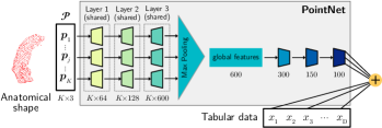
Figure 1: Wide and Deep PointNet Architecture (adapted from [20]).

2.2 Shapley Value

Given a trained WDPN, $f:\mathbb{R}^{K\times 3}\times\mathbb{R}^{D}\rightarrow[0;1]$, we want to explain the predicted probability of AD for one particular input $\mathbf{z}=(\mathcal{P},\bm{x})$ by estimating the contribution individual points in the point cloud and clinical features have on the prediction. In particular, we propose to estimate the Shapley value [23], which we will define next.

We denote by $\mathcal{F}$ the set of all features comprising the input, and $\mathbf{z}_{\mathcal{S}}$ the subset indexed by $\mathcal{S}\subseteq\mathcal{F}$. Let $g:\mathbf{P}(\mathcal{F})\rightarrow\mathbb{R}$ be a set function defined on the power set of $\mathcal{F}$, with $g(\mathcal{S})\neq 0$, $g(\emptyset)=0$. The contribution of a set of features $\mathcal{S}$ on the prediction is given by the set function $g(\mathcal{S})=f(\mathbf{z}_{\mathcal{S}};\mathbf{z}_{\mathcal{F}\setminus\mathcal{S}}^{\text{bl}})-f(\mathbf{z}^{\text{bl}}),$ where the first term corresponds to the prediction of the model after replacing all features not in $\mathcal{S}$ with a baseline value from the vector $\mathbf{z}^{\text{bl}}$. The Shapley value for feature $i$ is defined as

$$s_{i}({\mathbf{z}}\,|\,{f})={\textstyle\frac{1}{|\mathcal{F}|!}\sum_{\mathcal{S}\subseteq\mathcal{F}\backslash\{i\}}|\mathcal{S}|!\cdot(|\mathcal{F}|-|\mathcal{S}|-1)!\left(g(\mathcal{S}\cup\{i\})-g(\mathcal{S})\right).}$$ (1)

Approximate Shapley Value.

Computing (1) exactly would require exponential many evaluations of the difference $\Delta_{i}=g(\mathcal{S}\cup\{i\})-g(\mathcal{S})$ for each feature $i$. Therefore, we employ the approximate Shapley value, first proposed for voting games in [8]. Let $\mathbb{E}_{k}(\Delta_{i})$ denote the marginal contribution of feature $i$, where the expectation is over all $\mathcal{S}$ with $|\mathcal{S}|=k$. By writing (1) in an alternative form where we explicitly sum over all sets $\mathcal{S}$ of equal size and noting that there are ${|\mathcal{F}|-1}\choose{k}$ possible sets of size $k$, we arrive at the approximate Shapley value $\bar{s}_{i}$:

$$s_{i}({\mathbf{z}}\,|\,{f}) =\frac{1}{|\mathcal{F}|!}\sum_{k=0}^{|\mathcal{F}|-1}\sum_{\begin{subarray}{c}\mathcal{S}\subseteq\mathcal{F}\backslash\{i\}\\ |\mathcal{S}|=k\end{subarray}}k!(|\mathcal{F}|-k-1)!\cdot\Delta_{i}\approx\frac{1}{|\mathcal{F}|}\sum_{k=0}^{|\mathcal{F}|-1}\mathbb{E}_{k}(\Delta_{i})=\bar{s}_{i}({\mathbf{z}}\,|\,{f}).$$ (2)

We will now focus on our main contribution to efficiently estimate the expectation

$$\mathbb{E}_{k}(\Delta_{i})=\mathbb{E}_{k}[f(\mathbf{z}_{\mathcal{S}\cup\{i\}};\mathbf{z}_{\mathcal{F}\setminus\mathcal{S}\cup\{i\}}^{\text{bl}})]-\mathbb{E}_{k}[f(\mathbf{z}_{\mathcal{S}};\mathbf{z}_{\mathcal{F}\setminus\mathcal{S}}^{\text{bl}})].$$ (3)

2.3 Efficient Estimation of the Approximate Shapley Value

Our main contribution is based on the observation that we can treat $\mathbf{z}_{\mathcal{S}}$ over all sets $\mathcal{S}$ of size $k$ as a source of aleatoric uncertainty, i.e., we are unsure about the input [1]. Then, the objective becomes propagating the aleatoric uncertainty through the network. This is a challenging task, because we need to create a version of the WDPN that is probabilistic and faithful to the original model. To this end, we propose a novel probabilistic WDPN, inspired by the Lightweight Probabilistic Deep Network (LPDN, [10]), that models aleatoric uncertainty by assuming inputs are comprised of independent univariate normal distributions, one for each feature. The resulting probabilistic WDPN directly outputs an estimate of $\mathbb{E}_{k}[f(\mathbf{z}_{\mathcal{S}};\mathbf{z}_{\mathcal{F}\setminus\mathcal{S}}^{\text{bl}})]$ for a fixed $k$. Next, we will propose a new set of layers to transform inputs into distributions over sets $\mathcal{S}$ of size $k$.

Probabilistic PointNet.

The first part of the network in Fig. 1 processes the point cloud. It consists of multiple fully-connected layers with ReLU activation and batch normalization, where weights are shared across points. For the initial linear layer with weights $\mathbf{W}$, the $m$-th output for the $j$-th point is $h_{jm}=\sum_{l=1}^{3}p_{jl}W_{lm}$. To make it probabilistic, we need to account for $\mathbf{p}_{j}$ being included in $\mathcal{S}$ randomly. Since each $\mathcal{S}$ is selected with probability ${{|\mathcal{F}|}\choose{k}}^{-1}$ and there are ${{|\mathcal{F}|-1}\choose{k-1}}$ sets $S$ containing $\mathbf{p}_{j}$, we have

$$\mathbb{E}_{k}[h_{jm}]=\sum_{\begin{subarray}{c}\mathcal{S}\subseteq\mathcal{F}\\ |\mathcal{S}|=k\end{subarray}}{{|\mathcal{F}|}\choose{k}}^{-1}{{|\mathcal{F}|-1}\choose{k-1}}h_{jm}=\frac{k}{|\mathcal{F}|}h_{jm}.$$ (4)

This is a well-known result from sampling theory [1, 7], which also tells us that $h_{jm}$ can be approximated with a normal distribution with mean (4) and variance

$$\mathbb{V}_{k}(h_{jm})=k\frac{|\mathcal{F}|-k}{|\mathcal{F}|-1}\left[\frac{1}{|\mathcal{F}|}\sum_{l=1}^{3}(p_{jl}W_{lm})^{2}-\left(\frac{1}{|\mathcal{F}|}h_{jm}\right)^{2}\right].$$ (5)

After the first linear layer each output unit is approximated by a normal distribution, and we can employ a LPDN for all subsequent layers, by replacing ReLU, batch-norm, and max-pooling with their respective probabilistic versions [10]. The final output of the probabilistic PointNet is a global descriptor of the whole point cloud, where each feature has a mean and a variance attached to it.

Probabilistic Wide and Deep PointNet.

The final step in estimating the expectation (3) is the integration of clinical markers with the latent point cloud representation (yellow node in Fig. 1). Both information is combined in a linear layer, for which we need to propagate uncertainty due to the distributions describing the point cloud, and due to $\mathcal{S}$ covering a subset of clinical markers. Since a linear layer is an associative operation, we can compute the sum over the latent point cloud features and the clinical features separately, before combining the respective results, thus we split the expectation (3) into $\mathbb{E}_{k}(\Delta_{i})=\mathbb{E}_{k}(\Delta_{i}^{\bm{x}})+\mathbb{E}_{k}(\Delta_{i}^{\mathcal{P}})$. To compute the expectation with respect to tabular data $\bm{x}$, we utilize that for a linear layer with bias $b$ and weights $\mathbf{w}\in\mathbb{R}^{D}$, $f(\bm{x})=b+\mathbf{w}^{\top}\bm{x}$, thus $\mathbb{E}_{k}(\Delta_{i}^{\bm{x}})=w_{i}x_{i}$, if feature $i$ is tabular and $\mathbb{E}_{k}(\Delta_{i}^{\bm{x}})=0$ otherwise. The uncertainty due to the latent point cloud features can be propagated by a linear probabilistic layer [10] with mean $\mu_{k}^{\mathcal{S}}$, yielding $\mathbb{E}_{k}[f(\mathbf{z}_{\mathcal{S}};\mathbf{z}_{\mathcal{F}\setminus\mathcal{S}}^{\text{bl}})]=\mu_{k}^{\mathcal{S}}$. Doing the same, but accounting for the inclusion of $i$ in $\mathcal{S}$, we have $\mathbb{E}_{k}[f(\mathbf{z}_{\mathcal{S}\cup\{i\}};\mathbf{z}_{\mathcal{F}\setminus\mathcal{S}\cup\{i\}}^{\text{bl}})]=\mu_{k}^{\mathcal{S}\cup\{i\}}$. Finally, we subtract both means yielding $\mathbb{E}_{k}(\Delta_{i}^{\mathcal{P}})=\mu_{k}^{\mathcal{S}\cup\{i\}}-\mu_{k}^{\mathcal{S}}$. As a result, we can estimate $\mathbb{E}_{k}(\Delta_{i})$ with only two forward-passes, while keeping $\mathbf{z}$ and $k=|\mathcal{S}|$ fixed.

Estimating the Approximate Shapley Value.

Equipped with an efficient way to estimate the expectation over a fixed number of features in $\mathcal{S}$, we can compute the difference in (3). For the first term, we only need a single forward pass through the probabilistic WDPN using the original input with all features. For the second term, we again need one forward pass, but without the contribution of the $i$-th feature, which is replaced by a baseline value. This value differs depending on whether the $i$-th feature is a point in the hippocampus or a clinical marker. Thus, the complexity to estimate the approximate Shapley value for all features in the input is $\mathcal{O}((D+|\mathcal{P}|)^{2})$. For high-dimensional inputs, we can further reduce the complexity by estimating the average in (2) via $M$ Monte Carlo samples, yielding $\mathcal{O}(M(D+|\mathcal{P}|))$.

Choosing a Baseline.

Selection of an appropriate baseline $\mathbf{z}^{\text{bl}}$ is crucial in obtaining semantically meaningful explanations, as the $i$-th Shapley value reflects the contribution of feature $i$ to the difference $f(\mathbf{z})-f(\mathbf{z}^{\text{bl}})=\sum_{i=1}^{|\mathcal{F}|}s_{i}({\mathbf{z}}\,|\,{f})$ [23]. Assuming no clinical marker has been zero-encoded, we can replace the original value with zero to eliminate its impact. If the $i$-th feature belongs to the point cloud, the situation is more nuanced. Using all-zeros would describe a point at the origin and Shapley values would explain the difference to the prediction made from the origin, which has no semantic meaning in the case of the hippocampus. We propose a better alternative by replacing it with a matching point from a hull containing all point clouds in the dataset. Our motivation for this approach is that it avoids erratic changes of the point cloud’s surface when inserting a point at the origin, and that it provides a common, semantically meaningful reference for all patients, which eases interpretation of explanations across multiple patients.

3 Experiments

In this section, we are evaluating the computational efficiency, approximation error, and semantics of SVEHNN compared to the exact Shapley value [23], Occlusion [27], and Shapley sampling [5]. Note that except for Occlusion, these methods have not been used to explain predictions from shape data before. For each method, we compare three different approaches to choosing the baseline value in point clouds: (i) moving a point to the origin (zero), and (ii) replacing a point by its matching point from the common hull (hull). We quantitatively assess differences with respect to the exact Shapley value in terms of mean squared error (MSE), Spearman rank correlation (SRC), and normalized discounted cumulative gain (NDCG, [15]). MSE captures the overall approximation error, SRC is a measure of agreement between rankings of features, and NDCG is similar to SRC, but penalizes errors in important features – according to the ground truth – more. For NDCG, we use the absolute Shapley value as importance measure. We run Shapley sampling [5] with $M=2,000$ Monte Carlo samples, which results in a runtime of $\mathcal{O}(|\mathcal{P}|M)$. Note that sampling usually requires $M\gg|\mathcal{P}|$ for a good approximation.

3.1 Synthetic Shape Data Set

To assess the approximation error compared to the exact Shapley value in a reasonable amount of time, we created a synthetic dataset of point clouds comprising 16 points ($|\mathcal{P}|=16$). This allows calculation of the exact Shapley values across all $2^{16-1}$ subsets of $\mathcal{P}$ and use it as ground truth. We use a binary PointNet classifier to distinguish point clouds of the characters ‘X’ and ‘I’.

Table 1: Mean difference to exact Shapley value across 100 synthetic point clouds with zero baseline. NE: Number of network evaluations for each example.

Method	MSE	SRC	NDCG	NE
Exact	0	1	1	65,538
Sampling	0.0008	0.9505	0.9986	32,000
Sampling	0.0340	0.5440	0.9481	512
Occlusion	16.1311	0.3180	0.8659	17
SVEHNN	0.0443	0.6918	0.9641	512

Results in Table 1 show that occlusion fails in all categories, except runtime efficiency. SVEHNN closely approximates the exact Shapley value in terms of MSE with less than 0.8% of network evaluations. Running Shapley sampling until convergence (second row) ranks slightly higher, but at more than 60 times the cost of SVEHNN, it is a high cost for an improvement of less than 0.035 in NDCG. When considering Shapley sampling with the same runtime as SVEHNN (third row), rank metrics drop below that of SVEHNN; the MSE remains lower, which is due to the Gaussian approximation of activations in probabilistic layers of SVEHNN. Overall, we can conclude that SVEHNN is computationally efficient with only a small loss in accuracy.

3.2 Alzheimer’s Disease Diagnosis

In this experiment, we use data from the Alzheimer’s Disease Neuroimaging Initiative [13]. Brain scans were processed with FreeSurfer [9] from which we obtained the surface of the left hippocampus, represented as a point cloud with 1024 points. For tabular clinical data, we use age, gender, education (in orthogonal polynomial coding), APOE4, FDG-PET, AV45-PET, A$\beta_{42}$, total tau (t-tau), and phosphorylated tau (p-tau). We account for non-linear age effects using a natural B-spline expansion with four degrees of freedom. We exclude patients diagnosed with mild cognitive impairment and train a WDPN [20] to tell healthy controls from patients with AD. Data is split into 1308 visits for training, 169 for hyper-parameter tuning, and 176 for testing; all visits from one subject are included in the same split. The WDPN achieves a balanced accuracy of 0.942 on the test data. We run SVEHNN with 150 Monte Carlo samples and the hull baseline.

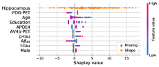
Figure 2: Shapley values of biomarkers and hippocampus shape of 167 correctly classified patients (dots, 110 healthy, 57 AD), sorted by mean relevance.

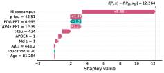
Figure 3: Shapley values of biomarkers of a single AD patient.

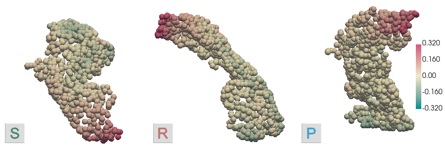
Figure 4: Shapley values of hippocampus shape of same patient as in Fig. 3. Left: Superior view. Middle: Right view. Right: Posterior view.

Figure 3 depicts the Shapley values of individual patients and features for all correctly classified test patients, sorted by the average feature relevance. For tabular biomarkers, colors indicate the range of feature values from low (blue) to high (red). For instance, APOE4 Shapley values of patients with no APOE4 allele are depicted in blue, with one allele in purple, and with two alleles in red. It shows that for a few patients the hippocampus shape is very important, whereas for most patients its relevance is similar to that of tabular biomarkers. Overall, relevance scores echo clinically validated results: high concentrations of p-tau/t-tau and APOE4 are markers for AD, whereas low levels of $A\beta_{42}$ and many years of education are protective [4, 11, 19]. To provide an example of a local explanation by SVEHNN, we selected one AD patient (see Fig. 3). It shows that the AD diagnosis was driven by the hippocampus shape, followed by p-tau, FDG-PET, and AV45-PET. The explanation of the hippocampus reveals that points located in the CA1 subfield were most important for diagnosis (see Fig. 4). This is reassuring, because atrophy in the CA1 subfield is an established marker for AD [14]. By cross-referencing the explanation with clinical knowledge, we can conclude that the predicted AD diagnosis is likely trustworthy.

4 Conclusion

Obtaining comprehensible and faithful explanations of decisions made by deep neural networks are paramount for the deployment of such systems in the clinic. We proposed a principled methodology for explaining individual predictions, which can help to build trust among the users of such a system. In this work, we studied explaining networks integrating neuroanatomical shape and tabular biomarkers, which has not been studied before. We followed an axiomatic approach based on the Shapley value – the unique procedure that satisfies all fundamental axioms of local explanation methods. Our proposed method Shapley Value Explanation of Heterogeneous Neural Networks (SVEHNN) closely approximates the exact Shapley value while requiring only a quadratic instead of exponential number of network evaluations. Finally, we illustrated how SVEHNN can help to understand Alzheimer’s diagnosis made by a network from heterogeneous data to reveal the hidden knowledge the network has learned from the data.

Acknowledgements.

This research was supported by the Bavarian State Ministry of Science and the Arts and coordinated by the Bavarian Research Institute for Digital Transformation, and the Federal Ministry of Education and Research in the call for Computational Life Sciences (DeepMentia, 031L0200A).

References

- [1] Ancona, M., Oztireli, C., Gross, M.: Explaining deep neural networks with a polynomial time algorithm for shapley value approximation. In: Proc. of the 36th International Conference on Machine Learning. vol. 97, pp. 272–281 (2019)
- [2] Arrieta, A.B., Díaz-Rodríguez, N., Ser, J.D., Bennetot, A., Tabik, S., Barbado, A., et al.: Explainable Artificial Intelligence (XAI): Concepts, taxonomies, opportunities and challenges toward responsible AI. Information Fusion 58, 82–115 (Jun 2020). https://doi.org/10.1016/j.inffus.2019.12.012
- [3] Bach, S., Binder, A., Montavon, G., Klauschen, F., Müller, K.R., Samek, W.: On Pixel-Wise Explanations for Non-Linear Classifier Decisions by Layer-Wise Relevance Propagation. PLOS ONE 10(7), e0130140 (Jul 2015). https://doi.org/10.1371/journal.pone.0130140
- [4] Blennow, K., Vanmechelen, E., Hampel, H.: CSF Total tau, A42 and Phosphorylated tau Protein as Biomarkers for Alzheimer’s Disease. Molecular Neurobiology 24(1-3), 087–098 (2001). https://doi.org/10.1385/mn:24:1-3:087
- [5] Castro, J., Gómez, D., Tejada, J.: Polynomial calculation of the Shapley value based on sampling. Computers & Operations Research 36(5), 1726–1730 (2009). https://doi.org/10.1016/j.cor.2008.04.004
- [6] Ching, T., Himmelstein, D.S., Beaulieu-Jones, B.K., Kalinin, A.A., Do, B.T., Way, G.P., Ferrero, E., et al.: Opportunities and obstacles for deep learning in biology and medicine. Journal of The Royal Society Interface 15(141), 20170387 (Apr 2018). https://doi.org/10.1098/rsif.2017.0387
- [7] Cochran: Sampling Techniques. John Wiley & Sons, 3rd edn. (1977)
- [8] Fatima, S.S., Wooldridge, M., Jennings, N.R.: A linear approximation method for the Shapley value. Artificial Intelligence 172(14), 1673–1699 (Sep 2008). https://doi.org/10.1016/j.artint.2008.05.003
- [9] Fischl, B.: FreeSurfer. NeuroImage 62(2), 774–781 (2012). https://doi.org/10.1016/j.neuroimage.2012.01.021
- [10] Gast, J., Roth, S.: Lightweight Probabilistic Deep Networks. In: The IEEE Conference on Computer Vision and Pattern Recognition (CVPR). pp. 3369–3378 (2018)
- [11] Genin, E., Hannequin, D., Wallon, D., Sleegers, K., Hiltunen, M., Combarros, O., et al.: APOE and Alzheimer disease: a major gene with semi-dominant inheritance. Molecular Psychiatry 16(9), 903–907 (2011). https://doi.org/10.1038/mp.2011.52
- [12] Gutiérrez-Becker, B., Wachinger, C.: Deep multi-structural shape analysis: application to neuroanatomy. In: Medical Image Computing and Computer Assisted Intervention (MICCAI). pp. 523–531 (2018). https://doi.org/10.1007/978-3-030-00931-1_60
- [13] Jack, C.R., Bernstein, M.A., Fox, N.C., Thompson, P., Alexander, G., Harvey, D., Borowski, B., Britson, P.J., et al.: The Alzheimer’s disease neuroimaging initiative (ADNI): MRI methods. Journal of Magnetic Resonance Imaging 27(4), 685–691 (2008). https://doi.org/10.1002/jmri.21049
- [14] Joie, R.L., Perrotin, A., de La Sayette, V., Egret, S., Doeuvre, L., et al.: Hippocampal subfield volumetry in mild cognitive impairment, Alzheimer’s disease and semantic dementia. NeuroImage: Clinical 3, 155–162 (2013). https://doi.org/10.1016/j.nicl.2013.08.007
- [15] Järvelin, K., Kekäläinen, J.: Cumulated gain-based evaluation of IR techniques. ACM Transactions on Information Systems (TOIS) 20(4), 422–446 (2002). https://doi.org/10.1145/582415.582418
- [16] Kopper, P., Pölsterl, S., Wachinger, C., Bischl, B., Bender, A., Rügamer, D.: Semi-structured deep piecewise exponential models. In: Proceedings of AAAI Spring Symposium on Survival Prediction - Algorithms, Challenges, and Applications 2021. vol. 146, pp. 40–53 (2021)
- [17] Li, X., Dvornek, N.C., Zhuang, J., Ventola, P., Duncan, J.S.: Brain Biomarker Interpretation in ASD Using Deep Learning and fMRI. In: Medical Image Computing and Computer Assisted Intervention (MICCAI). pp. 206–214 (2018). https://doi.org/10.1007/978-3-030-00931-1_24
- [18] Lundberg, S.M., Lee, S.I.: A Unified Approach to Interpreting Model Predictions. In: Advances in Neural Information Processing Systems 30. pp. 4765–4774 (2017)
- [19] Meng, X., D’Arcy, C.: Education and Dementia in the Context of the Cognitive Reserve Hypothesis: A Systematic Review with Meta-Analyses and Qualitative Analyses. PLoS ONE 7(6), e38268 (2012). https://doi.org/10.1371/journal.pone.0038268
- [20] Pölsterl, S., Sarasua, I., Gutiérrez-Becker, B., Wachinger, C.: A Wide and Deep Neural Network for Survival Analysis from Anatomical Shape and Tabular Clinical Data. In: Machine Learning and Knowledge Discovery in Databases. pp. 453–464 (2020). https://doi.org/10.1007/978-3-030-43823-4_37
- [21] Qi, C.R., Su, H., Mo, K., Guibas, L.J.: PointNet: Deep Learning on Point Sets for 3D Classification and Segmentation. In: The IEEE Conference on Computer Vision and Pattern Recognition (CVPR). pp. 652–660 (2017)
- [22] Selvaraju, R.R., Cogswell, M., Das, A., Vedantam, R., Parikh, D., Batra, D.: Grad-CAM: Visual Explanations from Deep Networks via Gradient-Based Localization. In: The IEEE International Conference on Computer Vision (ICCV) (2017). https://doi.org/10.1109/iccv.2017.74
- [23] Shapley, L.S.: A value for n-person games. Contributions to the Theory of Games 2(28), 307–317 (1953)
- [24] Shrikumar, A., Greenside, P., Kundaje, A.: Learning Important Features Through Propagating Activation Differences. In: Proc. of the 34th International Conference on Machine Learning. vol. 70, pp. 3145–3153 (2017)
- [25] Sundararajan, M., Najmi, A.: The many Shapley values for model explanation. In: Proc. of the 37th International Conference on Machine Learning. vol. 119, pp. 9269–9278 (2020)
- [26] Sundararajan, M., Taly, A., Yan, Q.: Axiomatic Attribution for Deep Networks. In: Proc. of the 34th International Conference on Machine Learning. vol. 70, pp. 3319–3328 (2017)
- [27] Zeiler, M.D., Fergus, R.: Visualizing and Understanding Convolutional Networks. In: European Conference on Computer Vision (ECCV). pp. 818–833 (2014)
- [28] Zhao, G., Zhou, B., Wang, K., Jiang, R., Xu, M.: Respond-CAM: Analyzing Deep Models for 3D Imaging Data by Visualizations. In: Medical Image Computing and Computer Assisted Intervention (MICCAI). pp. 485–492 (2018). https://doi.org/10.1007/978-3-030-00928-1_55
- [29] Zhuang, J., Dvornek, N.C., Li, X., Ventola, P., Duncan, J.S.: Invertible Network for Classification and Biomarker Selection for ASD. In: Medical Image Computing and Computer Assisted Intervention (MICCAI). pp. 700–708 (2019). https://doi.org/10.1007/978-3-030-32248-9_78