IID Sampling from Intractable Distributions

Abstract

In this article, we propose a novel methodology for drawing $iid$ realizations from any target distribution on the $d$-dimensional Euclidean space, for any $d\geq 1$. No assumption of compact support is necessary for the validity of our theory and method. The key idea is to construct an infinite sequence of concentric closed ellipsoids in keeping with the insight that the central one tends to support the modal region while the regions between successive concentric ellipsoids (ellipsoidal annuli) increasingly tend to support the tail regions of the target distribution as the sequence progresses.

Representing the target distribution as an infinite mixture of distributions on the central ellipsoid and the ellipsoidal annuli, we propose simulation from the mixture by selecting a mixture component with the relevant mixing probability, and then simulating from the mixture component via perfect simulation. We develop the perfect sampling scheme by first developing a minorization inequality of the general Metropolis-Hastings algorithm driven by uniform proposal distributions on the compact central ellipsoid and the annuli.

In contrast with most of the existing works on perfect sampling, ours is not only a theoretically valid method, it is practically applicable to all target distributions on any dimensional Euclidean space and very much amenable to parallel computation. We validate the practicality and usefulness of our methodology by generating $10000$ $iid$ realizations from the standard distributions such as normal, Student’s $t$ with $5$ degrees of freedom and Cauchy, for dimensions $d=1,5,10,50,100$, as well as from a $50$-dimensional mixture normal distribution. The implementation time in all the cases are very reasonable, and often less than a minute in our parallel implementation. The results turned out to be highly accurate.

We also apply our method to draw $10000$ $iid$ realizations from the posterior distributions associated with the well-known Challenger data, a Salmonella data and the $160$-dimensional challenging spatial example of the radionuclide count data on Rongelap Island. Again, we are able to obtain quite encouraging results with very reasonable computing time.
Keywords: Ellipsoid; Minorization; Parallel computing; Perfect sampling; Residual distribution; Transformation based Markov Chain Monte Carlo.

1 Introduction

That Markov Chain Monte Carlo (MCMC) has revolutionized Bayesian computation, is an understatement. But in spite of this, MCMC seems to be losing its charm, slowly but steadily, due to the challenges in ascertaining its convergence in practice. Even the most experienced MCMC theorists and practitioners are tending to give up on MCMC and looking for deterministic or even ad-hoc approximations to the posteriors on account of the challenges posed by MCMC, which they feel insurmountable.

The concept of perfect simulation, introduced by Propp and Wilson (1996), seemed promising initially to the MCMC community for solving the convergence problem. Yet, apparent infeasibility of direct practical implementation of the concept in general Bayesian problems managed to act as a deterrent to the community, to the extent of disbelief. So much so, that when the article Mukhopadhyay and Bhattacharya (2012), on perfect sampling in the mixture context, was initially submitted to a so-called reputed journal, the reaction of the reviewers was rejection on account of essentially total disbelief in the success of the idea (one of them even remarked that the work was “too ambitious”). As such, we are not aware of any promising research on perfect sampling in the recent years.

In this article, we take up the task of producing $iid$ realizations from any target distribution on $\mathbb{R}^{d}$, where $\mathbb{R}$ is the real line and $d\geq 1$. Our key idea revolves around judicious construction of an infinite sequence of closed ellipsoids, and representing the target distribution as an infinite mixture on the central ellipsoid and the regions between successive concentric ellipsoids (ellipsoidal annuli). This construction is a reflection of our insight that the central ellipsoid essentially tends to support the modal region and the annuli tend to support the tail regions of the target distribution.

Our proposal for generating $iid$ realizations hinges on drawing a mixture component with the relevant mixing probability, and the ability to simulate from the chosen component using a perfect sampling scheme. To develop the perfect sampling mechanism, we first consider the general Metropolis-Hastings algorithm on our compact ellipsoids and annuli, driven by uniform proposal distributions on these compact sets. Exploiting compactness, we then develop an appropriate minorization inequality for any given compact set in our sequence. Then representing the Metropolis-Hastings chain as a mixture of two components on any given member of our set sequence, we construct a perfect sampler for the mixture component density on its relevant support set. Furthermore, adopting and rectifying an idea proposed in Murdoch and Green (1998), we avoid the computationally expensive coupling from the past (CFTP) algorithm proposed in Propp and Wilson (1996). Bypassing CFTP rendered our perfect sampling idea very much computationally feasible. Integrating all our ideas, we develop a generic parallel algorithm for simulating $iid$ realizations from general target distributions.

To demonstrate the validity and feasibility of our developments in practice, we apply our parallel algorithm to some standard distributions: normal, Student’s $t$ with $5$ degrees of freedom and Cauchy, for dimensions $d=1,5,10,50,100$. We also apply our ideas to a $50$-dimensional mixture normal distribution. In each case, we consider an appropriate location vector and scale matrix. In all the aforementioned setups, we simulate $10000$ $iid$ realizations with our parallel algorithm, and the results are highly accurate. Moreover, the implementation times turned out to be very reasonable, and several of the exercises took less than a minute for completion.

Further, we apply our $iid$ method to posterior distributions based on real data. Specifically, we obtain $10000$ $iid$ realizations from the posteriors corresponding to the well-known Challenger data and the Salmonella data, consisting of two and three parameters, respectively. Finally, we generate $10000$ $iid$ realizations from the $160$-dimensional posterior distribution corresponding to the highly challenging spatial example of the radionuclide count data on Rongelap Island. The spatial example is considered to be an extremely daunting MCMC convergence problem, yet we are able to obtain $10000$ $iid$ samples in just $30$ minutes. As we demonstrate, all our results are highly reliable.

The rest of our article is organized as follows. We introduce our key idea in Section 2. The set-wise perfect sampling theory and method are developed in Section 3. In Section 4 we present our complete parallel algorithm for $iid$ sampling from general target distributions. Our experiments with $iid$ simulations from standard univariate and multivariate distributions are detailed in Section 5, and in Section 6 we provide details of our experiments on $iid$ simulations from posterior distributions based on real data. Finally, we summarize our ideas and make concluding remarks in Section 7.

2 The $iid$ sampling idea

Let $\pi(\boldsymbol{\theta})$ be the target distribution supported on $\mathbb{R}^{d}$, where $d\geq 1$. Here $\boldsymbol{\theta}=(\theta_{1},\ldots,\theta_{d})^{T}$. Note that the distribution can be represented as

$$\pi(\boldsymbol{\theta})=\sum_{i=1}^{\infty}\pi(\boldsymbol{A}_{i})\pi_{i}(\boldsymbol{\theta}),$$ (1)

where $\boldsymbol{A}_{i}$ are disjoint compact subsets of $\mathbb{R}^{d}$ such that $\cup_{i=1}^{\infty}\boldsymbol{A}_{i}=\mathbb{R}^{d}$, and

$$\pi_{i}(\boldsymbol{\theta})=\frac{\pi(\boldsymbol{\theta})}{\pi(\boldsymbol{A}_{i})}I_{\boldsymbol{A}_{i}}(\boldsymbol{\theta}),$$ (2)

is the distribution of $\boldsymbol{\theta}$ restricted on $\boldsymbol{A}_{i}$; $I_{\boldsymbol{A}_{i}}$ being the indicator function of $\boldsymbol{A}_{i}$. In (1), $\pi(\boldsymbol{A}_{i})=\int_{\boldsymbol{A}_{i}}\pi(d\boldsymbol{\theta})\geq 0$. Clearly, $\sum_{i=1}^{\infty}\pi(\boldsymbol{A}_{i})=1$.

The key idea of generating $iid$ realizations from $\pi(\boldsymbol{\theta})$ is to randomly select $\pi_{i}$ with probability $\pi(\boldsymbol{A}_{i})$ and then to perfectly simulate from $\pi_{i}$.

2.1 Choice of the sets $\boldsymbol{A}_{i}$

For some appropriate $d$-dimensional vector $\boldsymbol{\mu}$ and $d\times d$ positive definite scale matrix $\boldsymbol{\Sigma}$, we shall set $\boldsymbol{A}_{i}=\{\boldsymbol{\theta}:c_{i-1}\leq(\boldsymbol{\theta}-\boldsymbol{\mu})^{T}\boldsymbol{\Sigma}^{-1}(\boldsymbol{\theta}-\boldsymbol{\mu})\leq c_{i}\}$ for $i=1,2,\ldots$, where $0=c_{0}<c_{1}<c_{2}<\cdots$. Note that $\boldsymbol{A}_{1}=\{\boldsymbol{\theta}:(\boldsymbol{\theta}-\boldsymbol{\mu})^{T}\boldsymbol{\Sigma}^{-1}(\boldsymbol{\theta}-\boldsymbol{\mu})\leq c_{1}\}$, and for $i\geq 2$, $\boldsymbol{A}_{i}=\{\boldsymbol{\theta}:(\boldsymbol{\theta}-\boldsymbol{\mu})^{T}\boldsymbol{\Sigma}^{-1}(\boldsymbol{\theta}-\boldsymbol{\mu})\leq c_{i}\}\setminus\cup_{j=1}^{i-1}\boldsymbol{A}_{j}$. Observe that ideally one should set $\boldsymbol{A}_{i}=\{\boldsymbol{\theta}:c_{i-1}<(\boldsymbol{\theta}-\boldsymbol{\mu})^{T}\boldsymbol{\Sigma}^{-1}(\boldsymbol{\theta}-\boldsymbol{\mu})\leq c_{i}\}$, but since $\boldsymbol{\theta}$ has continuous distribution in our setup, we shall continue with $\boldsymbol{A}_{i}=\{\boldsymbol{\theta}:c_{i-1}\leq(\boldsymbol{\theta}-\boldsymbol{\mu})^{T}\boldsymbol{\Sigma}^{-1}(\boldsymbol{\theta}-\boldsymbol{\mu})\leq c_{i}\}$.

Thus, the first member of the sequence of sets $\boldsymbol{A}_{i}$; $i\geq 1$, is a closed ellipsoid, while the others are closed annuli, the regions between two successive concentric closed ellipsoids. The compact ellipsoid $\boldsymbol{A}_{1}$ tends to support the modal region of the target distribution $\pi$ and for increasing $i\geq 2$, the compact annuli $\boldsymbol{A}_{i}$ tend to support the tail regions of the target distribution. Thus in practice, it is useful to choose $\sqrt{c_{1}}$ associated with $\boldsymbol{A}_{1}$ to be relatively large compared to $\sqrt{c_{i}}$ for $i\geq 2$. As will be seen in Section 2.3.1, for $i\geq 1$, $\sqrt{c_{i}}$ are the radii of $d$-dimensional balls of the form $\left\{\boldsymbol{Y}:\boldsymbol{Y}^{T}\boldsymbol{Y}\leq c_{i}\right\}$ which has linear correspondence with $d$-dimensional ellipsoids of the form $\{\boldsymbol{\theta}:(\boldsymbol{\theta}-\boldsymbol{\mu})^{T}\boldsymbol{\Sigma}^{-1}(\boldsymbol{\theta}-\boldsymbol{\mu})\leq c_{i}\}$. Hence, we shall refer to $\sqrt{c_{i}}$; $i\geq 1$, as radii.

2.2 Choice of $\boldsymbol{\mu}$ and $\boldsymbol{\Sigma}$

Theoretically, any choice of $\boldsymbol{\mu}\in\mathbb{R}^{d}$ and any $d\times d$ positive definite scale matrix $\boldsymbol{\Sigma}$ is valid for our method. However, judicious choices of $\boldsymbol{\mu}$ and $\boldsymbol{\Sigma}$ play important roles in the efficiency of our $iid$ algorithm. In this regard, in practice, $\boldsymbol{\mu}$ and $\boldsymbol{\Sigma}$ will be the estimates of the mean (if it exists, or co-ordinate-wise median otherwise) and covariance structure of $\pi$ (it it exists, or some appropriate scale matrix otherwise). These estimates will be assumed to be obtained from some reliably implemented efficient MCMC algorithm. In this regard, we recommend the transformation based Markov Chain Monte Carlo (TMCMC) methodology introduced by Dutta and Bhattacharya (2014) that simultaneously updates all the variables using suitable deterministic transformations of some low-dimensional (often one-dimensional) random variable defined on some relevant support. Since the method is driven by the low-dimensional random variable, this leads to drastic dimension reduction in effect, with great improvement in acceptance rates and computational efficiency, while ensuring adequate convergence properties. Our experiences also reveal that addition of a further deterministic step to TMCMC, in a similar vein as in Liu and Sabatti (2000) often dramatically enhances the convergence properties of TMCMC.

2.3 Dealing with the mixing probabilities $\pi(\boldsymbol{A}_{i})$

Recall that the key idea of $iid$ sampling from $\pi(\boldsymbol{\theta})$ is to randomly select $\pi_{i}$ with probability $\pi(\boldsymbol{A}_{i})$ and then to exactly simulate from $\pi_{i}$. However, the mixing probabilities $\pi(\boldsymbol{A}_{i})$ are not available prior to simulation. Since there are infinite number of such probabilities, even estimation of all these probabilities using only a finite TMCMC sample from $\pi$ is out of the question. But estimation of $\pi(\boldsymbol{A}_{i})$ using Monte Carlo samples drawn uniformly from $\boldsymbol{A}_{i}$ makes sense, and the strategy applies to all $i\geq 1$. For the time being assume that we have an infinite number of parallel processors, and the $i$-th processor is used to estimate $\pi(\boldsymbol{A}_{i})$ using Monte Carlo sampling up to a constant. To elaborate, let $\pi(\boldsymbol{\theta})=C\tilde{\pi}(\boldsymbol{\theta})$, where $C>0$ is the unknown normalizing constant. Then for any Borel set $\boldsymbol{A}$ in the Borel $\sigma$-field of $\mathbb{R}^{d}$, letting $\mathcal{L}(\boldsymbol{A})$ denote the Lebesgue measure of $\boldsymbol{A}$, observe that

$$\pi(\boldsymbol{A}_{i})=C\mathcal{L}(\boldsymbol{A}_{i})\int\tilde{\pi}(\boldsymbol{\theta})\frac{1}{\mathcal{L}(\boldsymbol{A}_{i})}I_{\boldsymbol{A}_{i}}(\boldsymbol{\theta})d\boldsymbol{\theta}=C\mathcal{L}(\boldsymbol{A}_{i})E\left[\tilde{\pi}(\boldsymbol{\theta})\right],$$ (3)

the right hand side being $C\mathcal{L}(\boldsymbol{A}_{i})$ times the expectation of $\tilde{\pi}(\boldsymbol{\theta})$ with respect to the uniform distribution on $\boldsymbol{A}_{i}$. This expectation can be estimated by generating realizations of $\boldsymbol{\theta}$ from the uniform distribution on $\boldsymbol{A}_{i}$, evaluating $\tilde{\pi}(\boldsymbol{\theta})$ for the realizations and taking their average. Let $\widehat{\tilde{\pi}(\boldsymbol{A}_{i})}$ denote the Monte Carlo average times $\mathcal{L}(\boldsymbol{A}_{i})$, so that $\widehat{\tilde{\pi}(\boldsymbol{A}_{i})}$ is an estimate of $\tilde{\pi}(\boldsymbol{A}_{i})$. The required uniform sample generation from $\boldsymbol{A}_{i}$ and computation of $\mathcal{L}(\boldsymbol{A}_{i})$ can be achieved in straightforward ways, which we elucidate below.

2.3.1 Uniform sampling from $\boldsymbol{A}_{i}$

First consider uniform generation from the $d$-dimensional ball $\{\boldsymbol{Y}:\boldsymbol{Y}^{T}\boldsymbol{Y}\leq c_{1}\}$, which consists of generation of $X_{k}\stackrel{{\scriptstyle iid}}{{\sim}}N(0,1)$, for $k=1,\ldots,d$, $U\sim U(0,1)$, the uniform distribution on $[0,1]$, and setting $\boldsymbol{Y}=\sqrt{c_{1}}U^{1/d}\boldsymbol{X}/\|\boldsymbol{X}\|$, where $\boldsymbol{X}=(X_{1},\ldots,X_{d})^{T}$ and $\|\cdot\|$ is the Euclidean norm. Then, letting $\boldsymbol{\Sigma}=\boldsymbol{B}\boldsymbol{B}^{T}$, where $\boldsymbol{B}$ is the lower triangular Cholesky factor of $\boldsymbol{\Sigma}$, $\boldsymbol{\theta}=\boldsymbol{\mu}+\boldsymbol{B}\boldsymbol{Y}$ is a uniform realization from $\boldsymbol{A}_{1}$. To generate uniformly from $\boldsymbol{A}_{i}=\{\boldsymbol{\theta}:c_{i-1}\leq(\boldsymbol{\theta}-\boldsymbol{\mu})^{T}\boldsymbol{\Sigma}^{-1}(\boldsymbol{\theta}-\boldsymbol{\mu})\leq c_{i}\}=\{\boldsymbol{\theta}:(\boldsymbol{\theta}-\boldsymbol{\mu})^{T}\boldsymbol{\Sigma}^{-1}(\boldsymbol{\theta}-\boldsymbol{\mu})\leq c_{i}\}\setminus\{\boldsymbol{\theta}:(\boldsymbol{\theta}-\boldsymbol{\mu})^{T}\boldsymbol{\Sigma}^{-1}(\boldsymbol{\theta}-\boldsymbol{\mu})\leq c_{i-1}\}$ for $i\geq 2$, we shall continue uniform simulation of $\tilde{\boldsymbol{\theta}}$ from $\{\boldsymbol{\theta}:(\boldsymbol{\theta}-\boldsymbol{\mu})^{T}\boldsymbol{\Sigma}^{-1}(\boldsymbol{\theta}-\boldsymbol{\mu})\leq c_{i}\}$ until $\tilde{\boldsymbol{\theta}}$ satisfies $(\tilde{\boldsymbol{\theta}}-\boldsymbol{\mu})^{T}\boldsymbol{\Sigma}^{-1}(\tilde{\boldsymbol{\theta}}-\boldsymbol{\mu})>c_{i-1}$.

Note that this basic rejection sampling scheme will be inefficient with high rejection probabilities for $i\geq 2$ when $\sqrt{c_{i}}-\sqrt{c_{i-1}}$ are very small. In such cases, it is important to replace this algorithm with methods that avoid the rejection mechanism. We indeed devise such a method for situations with small $\sqrt{c_{i}}-\sqrt{c_{i-1}}$ for $i\geq 2$ that completely bypasses rejection sampling; see Section 6.

2.3.2 Lebesgue measure of $\boldsymbol{A}_{i}$

It is well-known (see, for example, Giraud (2015)) that the volume of a $d$-dimensional ball of radius $c$ is given by $\frac{\pi^{d/2}}{\Gamma(d/2+1)}c^{d}$, where $\Gamma(x)=\int_{0}^{\infty}t^{x-1}\exp(-t)dt$, for $x>0$, is the Gamma function. Hence, in our case, letting $|\boldsymbol{B}|$ denote the determinant of $\boldsymbol{B}$,

$$\mathcal{L}(\boldsymbol{A}_{1})=|\boldsymbol{B}|\times\mathcal{L}(\{\boldsymbol{\theta}:\|\boldsymbol{\theta}\|\leq\sqrt{c_{1}}\})=\frac{|\boldsymbol{B}|\pi^{d/2}}{\Gamma(d/2+1)}c^{d/2}_{1},$$

and for $i\geq 2$, $\boldsymbol{A}_{i}$ has Lebesgue measure

$$\mathcal{L}(\boldsymbol{A}_{i}) =|\boldsymbol{B}|\times\mathcal{L}(\{\boldsymbol{\theta}:\|\boldsymbol{\theta}\|\leq\sqrt{c_{i}}\})-|\boldsymbol{B}|\times\mathcal{L}(\{\boldsymbol{\theta}:\|\boldsymbol{\theta}\|\leq\sqrt{c_{i-1}}\})$$

$$=|\boldsymbol{B}|\times\frac{\pi^{d/2}}{\Gamma(d/2+1)}\left(c^{d/2}_{i}-c^{d/2}_{i-1}\right).$$

The aforementioned ideas show that all the estimates $\widehat{\tilde{\pi}(\boldsymbol{A}_{i})}$, for $i\geq 1$, are obtainable simultaneously by parallel processing. Also assume that the Monte Carlo sample size $N_{i}$ is large enough for each $i$ such that for any $\epsilon>0$,

$$1-\epsilon\leq\frac{\tilde{\pi}(\boldsymbol{A}_{i})}{\widehat{\tilde{\pi}(\boldsymbol{A}_{i})}}\leq 1+\epsilon.$$ (4)

We further assume that depending on $\epsilon$, there exists $M_{0}\geq 1$ such that for all $M\geq M_{0}$,

$$1-\epsilon\leq C\sum_{i=1}^{M}\widehat{\tilde{\pi}(\boldsymbol{A}_{i})}\leq 1+\epsilon.$$ (5)

Letting

$$\hat{\pi}(\boldsymbol{\theta})=C\sum_{i=1}^{\infty}\widehat{\tilde{\pi}(\boldsymbol{A}_{i})}\pi_{i}(\boldsymbol{\theta}),$$ (6)

which is a well-defined density due to (5), we next provide a rejection sampling based argument to establish that it is sufficient to perfectly simulate from $\hat{\pi}(\boldsymbol{\theta})$ in order to sample perfectly from $\pi(\boldsymbol{\theta})$.

2.4 A rejection sampling argument for validation of $\hat{\pi}(\boldsymbol{\theta})$

Due to (4), for all $\boldsymbol{\theta}\in\mathbb{R}^{d}$,

$$\pi(\boldsymbol{\theta})=C\sum_{i=1}^{\infty}\widehat{\tilde{\pi}(\boldsymbol{A}_{i})}\times\frac{\tilde{\pi}(\boldsymbol{A}_{i})}{\widehat{\tilde{\pi}(\boldsymbol{A}_{i})}}\times\pi_{i}(\boldsymbol{\theta})\leq C(1+\epsilon)\sum_{i=1}^{\infty}\widehat{\tilde{\pi}(\boldsymbol{A}_{i})}\pi_{i}(\boldsymbol{\theta})=(1+\epsilon)\hat{\pi}(\boldsymbol{\theta}).$$

That is, for all $\boldsymbol{\theta}\in\mathbb{R}^{d}$,

$$\frac{\pi(\boldsymbol{\theta})}{\hat{\pi}(\boldsymbol{\theta})}\leq 1+\epsilon,$$ (7)

showing that rejection sampling is applicable for generating samples from $\pi(\boldsymbol{\theta})$ by sampling $\boldsymbol{\theta}$ from $\hat{\pi}(\boldsymbol{\theta})$ and generating $U\sim U(0,1)$ until the following is satisfied:

$$U<\frac{\pi(\boldsymbol{\theta})}{(1+\epsilon)\hat{\pi}(\boldsymbol{\theta})}.$$ (8)

In (8), $\boldsymbol{\theta}\in\boldsymbol{A}_{i}$ for some $i\geq 1$. Hence, due to (4),

$$\frac{\pi(\boldsymbol{\theta})}{(1+\epsilon)\hat{\pi}(\boldsymbol{\theta})}=\frac{1}{(1+\epsilon)}\frac{\tilde{\pi}(\boldsymbol{A}_{i})}{\widehat{\tilde{\pi}(\boldsymbol{A}_{i})}}>\frac{1-\epsilon}{1+\epsilon}.$$ (9)

The right most side of (9) can be made arbitrarily close to $1$ for sufficiently small $\epsilon>0$. Now, since $U\leq 1$ with probability $1$, this entails that (8) is satisfied with probability almost equal to one. Thus, for sufficiently small $\epsilon>0$, we can safely assume that (8) holds for all practical applications, so that any simulation of $\boldsymbol{\theta}$ from $\hat{\pi}(\boldsymbol{\theta})$ would be accepted in the rejection sampling step. In other words, to generate samples from the target density $\pi(\boldsymbol{\theta})$ it is sufficient to simply generate from $\hat{\pi}(\boldsymbol{\theta})$, for sufficiently small $\epsilon$.

3 Perfect sampling from $\hat{\pi}(\boldsymbol{\theta})$

For perfect sampling from $\hat{\pi}(\boldsymbol{\theta})$ we first need to select $\pi_{i}$ with probability $C\widehat{\tilde{\pi}(\boldsymbol{A}_{i})}$ for some $i\geq 1$, and then need to sample from $\pi_{i}$ in the perfect sense. Now $\pi_{i}$ would be selected if

$$\frac{\sum_{j=1}^{i-1}\widehat{\tilde{\pi}(\boldsymbol{A}_{j})}}{\sum_{j=1}^{\infty}\widehat{\tilde{\pi}(\boldsymbol{A}_{j})}}<U<\frac{\sum_{j=1}^{i}\widehat{\tilde{\pi}(\boldsymbol{A}_{j})}}{\sum_{j=1}^{\infty}\widehat{\tilde{\pi}(\boldsymbol{A}_{j})}},$$ (10)

where $U\sim U(0,1)$ and $\widehat{\tilde{\pi}(\boldsymbol{A}_{0})}=0$. But the denominator of the left and right hand sides of (10) involves an infinite sum, which can not be computed. However, note that due to (5),

$$1-\epsilon\leq\frac{\sum_{j=1}^{M}\widehat{\tilde{\pi}(\boldsymbol{A}_{j})}}{\sum_{j=1}^{\infty}\widehat{\tilde{\pi}(\boldsymbol{A}_{j})}}\leq 1+\epsilon.$$ (11)

The following hold due to (11):

$$(1-\epsilon)\frac{\sum_{j=1}^{i-1}\widehat{\tilde{\pi}(\boldsymbol{A}_{j})}}{\sum_{j=1}^{M}\widehat{\tilde{\pi}(\boldsymbol{A}_{j})}}\leq\frac{\sum_{j=1}^{i-1}\widehat{\tilde{\pi}(\boldsymbol{A}_{j})}}{\sum_{j=1}^{\infty}\widehat{\tilde{\pi}(\boldsymbol{A}_{j})}}\leq(1+\epsilon)\frac{\sum_{j=1}^{i-1}\widehat{\tilde{\pi}(\boldsymbol{A}_{j})}}{\sum_{j=1}^{M}\widehat{\tilde{\pi}(\boldsymbol{A}_{j})}};$$ (12)

$$(1-\epsilon)\frac{\sum_{j=1}^{i}\widehat{\tilde{\pi}(\boldsymbol{A}_{j})}}{\sum_{j=1}^{M}\widehat{\tilde{\pi}(\boldsymbol{A}_{j})}}\leq\frac{\sum_{j=1}^{i}\widehat{\tilde{\pi}(\boldsymbol{A}_{j})}}{\sum_{j=1}^{\infty}\widehat{\tilde{\pi}(\boldsymbol{A}_{j})}}\leq(1+\epsilon)\frac{\sum_{j=1}^{i}\widehat{\tilde{\pi}(\boldsymbol{A}_{j})}}{\sum_{j=1}^{M}\widehat{\tilde{\pi}(\boldsymbol{A}_{j})}}.$$ (13)

Due to (12) and (13), for sufficiently small $\epsilon>0$, in all practical implementations (10) holds if and only if

$$\frac{\sum_{j=1}^{i-1}\widehat{\tilde{\pi}(\boldsymbol{A}_{j})}}{\sum_{j=1}^{M}\widehat{\tilde{\pi}(\boldsymbol{A}_{j})}}<U<\frac{\sum_{j=1}^{i}\widehat{\tilde{\pi}(\boldsymbol{A}_{j})}}{\sum_{j=1}^{M}\widehat{\tilde{\pi}(\boldsymbol{A}_{j})}}$$ (14)

holds. If, in any case, $i=M$, then we shall compute $\widehat{\tilde{\pi}(\boldsymbol{A}_{j})}$; $j=M+1,\ldots,2M$, and re-check (14) for the same set of uniform random numbers $U\sim U(0,1)$ as before by replacing $M$ with $2M$, and continue the procedure until all the indices $i$ are less than $M$.

Once $\pi_{i}$ is selected by the above strategy, we can proceed to sample perfectly from $\pi_{i}$. We progress towards building an effective perfect sampling strategy by first establishing a minorization condition for the Markov transition kernel.

3.1 Minorization for $\pi_{i}$

For $\pi_{i}$, we consider the Metropolis-Hastings algorithm in which all the co-ordinates $\theta_{k}$; $k=1,\ldots,d$, are updated in a single block using an independence uniform proposal density on $\boldsymbol{A}_{i}$ given by

$$q_{i}(\boldsymbol{\theta}^{\prime})=\frac{1}{\mathcal{L}(\boldsymbol{A}_{i})}I_{\boldsymbol{A}_{i}}(\boldsymbol{\theta}^{\prime}).$$ (15)

Although independence proposal distributions are usually not recommended, particularly in high dimensions, here this makes good sense. Indeed, since $\boldsymbol{A}_{i}$ are so constructed that the densities $\pi_{i}$ are expected to be relatively flat on these sets, the uniform proposal is expected to provide good approximation to the target $\pi_{i}$. Furthermore, as we shall show, the uniform proposal will be responsible for obtaining significantly large lower bound for our minorization, which, in turn, will play the defining role in our construction of an efficient perfect sampler for $\pi_{i}$.

For $\boldsymbol{\theta}\in\boldsymbol{A}_{i}$, for any Borel set $\mathbb{B}$ in the Borel $\sigma$-field of $\mathbb{R}^{d}$, let $P_{i}(\boldsymbol{\theta},\mathbb{B}\cap\boldsymbol{A}_{i})$ denote the corresponding Metropolis-Hastings transition probability for $\pi_{i}$. Let $s_{i}=\underset{\boldsymbol{\theta}\in\boldsymbol{A}_{i}}{\inf}~{}\tilde{\pi}(\boldsymbol{\theta})$ and $S_{i}=\underset{\boldsymbol{\theta}\in\boldsymbol{A}_{i}}{\sup}~{}\tilde{\pi}(\boldsymbol{\theta})$. Then, with (15) as the proposal density we have

$$P_{i}(\boldsymbol{\theta},\mathbb{B}\cap\boldsymbol{A}_{i}) \geq\int_{\mathbb{B}\cap\boldsymbol{A}_{i}}\min\left\{1,\frac{\tilde{\pi}(\boldsymbol{\theta}^{\prime})}{\tilde{\pi}(\boldsymbol{\theta})}\right\}q_{i}(\boldsymbol{\theta}^{\prime})d\boldsymbol{\theta}^{\prime}$$

$$\geq\left(\frac{s_{i}}{S_{i}}\right)\times\frac{\mathcal{L}(\mathbb{B}\cap\boldsymbol{A}_{i})}{\mathcal{L}(\boldsymbol{A}_{i})}$$

$$=p_{i}~{}Q_{i}(\mathbb{B}\cap\boldsymbol{A}_{i}),$$ (16)

where $p_{i}=s_{i}/S_{i}$ and

$$Q_{i}(\mathbb{B}\cap\boldsymbol{A}_{i})=\frac{\mathcal{L}(\mathbb{B}\cap\boldsymbol{A}_{i})}{\mathcal{L}(\boldsymbol{A}_{i})}$$

is the uniform probability measure corresponding to (15). Since (16) holds for all $\boldsymbol{\theta}\in\boldsymbol{A}_{i}$, the entire set $\boldsymbol{A}_{i}$ is a small set.

Here are some important remarks regarding justification of the choice of the uniform proposal density. First, since the uniform proposal is the independence sampler, independent of the previous state of the underlying Markov chain, the right hand side of (16) is rendered independent of $\boldsymbol{\theta}$, which is a requisite condition for minorization. For proposal distributions of the form $q_{i}(\boldsymbol{\theta}^{\prime}|\boldsymbol{\theta})$, infimum of $q_{i}(\boldsymbol{\theta}^{\prime}|\boldsymbol{\theta})$ for $\boldsymbol{\theta},\boldsymbol{\theta}^{\prime}\in\boldsymbol{A}_{i}$ would be necessary, which would lead to much smaller lower bound for $P_{i}(\boldsymbol{\theta},\mathbb{B}\cap\boldsymbol{A}_{i})$ compared to the right hand side of (16). This is precisely the reason why we do not consider TMCMC for $iid$ sampling, whose move types depend upon the previous state. Any independence proposal density other than the uniform will not get cancelled in the Metropolis-Hastings acceptance ratio and the corresponding $s_{i}/S_{i}$ may be vanishingly small if $\tilde{\pi}$ is not well-approximated by the independence proposal on $\boldsymbol{A}_{i}$. This would make perfect sampling infeasible. Furthermore, as will be seen in Section 3.2, for perfect sampling it is required to simulate from the proposal density. But unlike the case of uniform proposal, it may be difficult to simulate from the proposal on $\boldsymbol{A}_{i}$, which has closed ellipsoidal or closed annulus structure.

Observe that $s_{i}$ and $S_{i}$ associated with (16) will usually not be available in closed forms. In this regard, let $\hat{s}_{i}$ and $\hat{S}_{i}$ denote the minimum and maximum of $\tilde{\pi}(\cdot)$ over the Monte Carlo samples drawn uniformly from $\boldsymbol{A}_{i}$ in course of estimating $\tilde{\pi}(\boldsymbol{A}_{i})$ by $\widehat{\tilde{\pi}(\boldsymbol{A}_{i})}$. Then $\frac{s_{i}}{S_{i}}\leq\frac{\hat{s}_{i}}{\hat{S}_{i}}$. Hence, there exists $\eta_{i}>0$ such that $1\geq\frac{s_{i}}{S_{i}}\geq\frac{\hat{s}_{i}}{\hat{S}_{i}}-\eta_{i}>0$. Let $\hat{p}_{i}=\frac{\hat{s}_{i}}{\hat{S}_{i}}-\eta_{i}$. Then it follows from (16) that

$$P_{i}(\boldsymbol{\theta},\mathbb{B}\cap\boldsymbol{A}_{i}\geq\hat{p}_{i}~{}Q_{i}(\mathbb{B}\cap\boldsymbol{A}_{i}),$$ (17)

which we shall consider for our purpose from now on. In practice, $\eta_{i}$ is expected to be very close to zero, since the Monte Carlo sample size would be sufficiently large. Thus, $\hat{p}_{i}$ is expected to be very close to $p_{i}$.

3.2 Split chain

Due to the minorization (17), $P_{i}(\boldsymbol{\theta},\mathbb{B}\cap\boldsymbol{A}_{i})$ admits the following decomposition for all $\boldsymbol{\theta}\in\boldsymbol{A}_{i}$:

$$P_{i}(\boldsymbol{\theta},\mathbb{B}\cap\boldsymbol{A}_{i})=\hat{p}_{i}~{}Q_{i}(\mathbb{B}\cap\boldsymbol{A}_{i})+(1-\hat{p}_{i})~{}R_{i}(\boldsymbol{\theta},\mathbb{B}\cap\boldsymbol{A}_{i}),$$ (18)

where

$$R_{i}(\boldsymbol{\theta},\mathbb{B}\cap\boldsymbol{A}_{i})=\frac{P_{i}(\boldsymbol{\theta},\mathbb{B}\cap\boldsymbol{A}_{i})-\hat{p}_{i}~{}Q_{i}(\mathbb{B}\cap\boldsymbol{A}_{i})}{1-\hat{p}_{i}}$$ (19)

is the residual distribution.

Therefore, to implement the Markov chain $P_{i}(\boldsymbol{\theta},\mathbb{B}\cap\boldsymbol{A}_{i})$, rather than proceeding directly with the uniform proposal based Metropolis-Hastings algorithm, we can use the split (18) to generate realizations from $P_{i}(\boldsymbol{\theta},\mathbb{B}\cap\boldsymbol{A}_{i})$. That is, given $\boldsymbol{\theta}$, we can simulate from $Q_{i}$ with probability $\hat{p}_{i}$, and with the remaining probability, can generate from $R_{i}(\boldsymbol{\theta},\cdot)$.

To simulate from the residual density $R_{i}(\boldsymbol{\theta},\cdot)$ we devise the following rejection sampling scheme. Let $\tilde{R}_{i}(\boldsymbol{\theta},\boldsymbol{\theta}^{\prime})$ and $\tilde{P}_{i}(\boldsymbol{\theta},\boldsymbol{\theta}^{\prime})$ denote the densities of $\boldsymbol{\theta}^{\prime}$ with respect to $R_{i}(\boldsymbol{\theta},\cdot)$ and $P_{i}(\boldsymbol{\theta},\cdot)$, respectively. Then it follows from (18) and (19) that for all $\boldsymbol{\theta}\in\boldsymbol{A}_{i}$,

$$\tilde{R}_{i}(\boldsymbol{\theta},\boldsymbol{\theta}^{\prime})=\frac{\tilde{P}_{i}(\boldsymbol{\theta},\boldsymbol{\theta}^{\prime})-\hat{p}_{i}~{}q_{i}(\boldsymbol{\theta}^{\prime})}{1-\hat{p}_{i}}\leq\frac{\tilde{P}_{i}(\boldsymbol{\theta},\boldsymbol{\theta}^{\prime})}{1-\hat{p}_{i}}$$

$$\Leftrightarrow\frac{\tilde{R}_{i}(\boldsymbol{\theta},\boldsymbol{\theta}^{\prime})}{\tilde{P}_{i}(\boldsymbol{\theta},\boldsymbol{\theta}^{\prime})}\leq\frac{1}{1-\hat{p}_{i}},~{}\mbox{for all}~{}\boldsymbol{\theta}^{\prime}\in\boldsymbol{A}_{i}.$$

Hence, given $\boldsymbol{\theta}$ we can continue to simulate $\boldsymbol{\theta}^{\prime}\sim\tilde{P}_{i}(\boldsymbol{\theta},\cdot)$ using the uniform proposal distribution (15) and generate $U\sim U(0,1)$ until

$$U<\frac{(1-\hat{p}_{i})\tilde{R}_{i}(\boldsymbol{\theta},\boldsymbol{\theta}^{\prime})}{\tilde{P}_{i}(\boldsymbol{\theta},\boldsymbol{\theta}^{\prime})}$$ (20)

is satisfied, at which point we accept $\boldsymbol{\theta}^{\prime}$ as a realization from $\tilde{R}_{i}(\boldsymbol{\theta},\cdot)$.

Now

$$\tilde{P}_{i}(\boldsymbol{\theta},\boldsymbol{\theta}^{\prime}) =q_{i}(\boldsymbol{\theta}^{\prime})\min\left\{1,\frac{\pi(\boldsymbol{\theta}^{\prime})}{\pi(\boldsymbol{\theta})}\right\}+r_{i}(\boldsymbol{\theta})I_{\boldsymbol{\theta}}(\boldsymbol{\theta}^{\prime})$$

$$=\frac{1}{\mathcal{L}(\boldsymbol{A}_{i})}\min\left\{1,\frac{\pi(\boldsymbol{\theta}^{\prime})}{\pi(\boldsymbol{\theta})}\right\}+r_{i}(\boldsymbol{\theta})I_{\boldsymbol{\theta}}(\boldsymbol{\theta}^{\prime}),$$

where

$$r_{i}(\boldsymbol{\theta}) =1-\int_{\boldsymbol{A}_{i}}\min\left\{1,\frac{\pi(\tilde{\boldsymbol{\theta}})}{\pi(\boldsymbol{\theta})}\right\}q_{i}(\tilde{\boldsymbol{\theta}})d\tilde{\boldsymbol{\theta}}$$

$$=1-\int_{\boldsymbol{A}_{i}}\min\left\{1,\frac{\pi(\tilde{\boldsymbol{\theta}})}{\pi(\boldsymbol{\theta})}\right\}\frac{1}{\mathcal{L}(\boldsymbol{A}_{i})}d\tilde{\boldsymbol{\theta}}.$$ (21)

Let $\hat{r}_{i}(\boldsymbol{\theta})$ denote the Monte Carlo estimate of $r_{i}(\boldsymbol{\theta})$ obtained by simulating $\tilde{\boldsymbol{\theta}}$ from the uniform distribution on $\boldsymbol{A}_{i}$ and taking the average of $\min\left\{1,\frac{\pi(\tilde{\boldsymbol{\theta}})}{\pi(\boldsymbol{\theta})}\right\}$ in (21). Let

$$\hat{P}_{i}(\boldsymbol{\theta},\boldsymbol{\theta}^{\prime}) =\frac{1}{\mathcal{L}(\boldsymbol{A}_{i})}\min\left\{1,\frac{\pi(\boldsymbol{\theta}^{\prime})}{\pi(\boldsymbol{\theta})}\right\}+\hat{r}_{i}(\boldsymbol{\theta})I_{\boldsymbol{\theta}}(\boldsymbol{\theta}^{\prime}),~{}\mbox{and}$$

$$\hat{R}_{i}(\boldsymbol{\theta},\boldsymbol{\theta}^{\prime}) =\frac{\hat{P}_{i}(\boldsymbol{\theta},\boldsymbol{\theta}^{\prime})-\hat{p}_{i}~{}q_{i}(\boldsymbol{\theta}^{\prime})}{1-\hat{p}_{i}}.$$

Given $\boldsymbol{\theta}$ and any $\epsilon>0$, let the Monte Carlo sample size be large enough such that

$$1-\epsilon\leq\frac{\tilde{P}_{i}(\boldsymbol{\theta},\boldsymbol{\theta}^{\prime})}{\hat{P}_{i}(\boldsymbol{\theta},\boldsymbol{\theta}^{\prime})}\leq 1+\epsilon,~{}\mbox{and}$$

$$1-\epsilon\leq\frac{\tilde{R}_{i}(\boldsymbol{\theta},\boldsymbol{\theta}^{\prime})}{\hat{R}_{i}(\boldsymbol{\theta},\boldsymbol{\theta}^{\prime})}\leq 1+\epsilon.$$

Then

$$\left(\frac{1-\epsilon}{1+\epsilon}\right)\frac{\tilde{R}_{i}(\boldsymbol{\theta},\boldsymbol{\theta}^{\prime})}{\tilde{P}_{i}(\boldsymbol{\theta},\boldsymbol{\theta}^{\prime})}\leq\frac{\hat{R}_{i}(\boldsymbol{\theta},\boldsymbol{\theta}^{\prime})}{\hat{P}_{i}(\boldsymbol{\theta},\boldsymbol{\theta}^{\prime})}\leq\left(\frac{1+\epsilon}{1-\epsilon}\right)\frac{\tilde{R}_{i}(\boldsymbol{\theta},\boldsymbol{\theta}^{\prime})}{\tilde{P}_{i}(\boldsymbol{\theta},\boldsymbol{\theta}^{\prime})}.$$ (22)

Due to (22), in all practical implementations, for sufficiently small $\epsilon>0$, (20) holds if and only if

$$U<\frac{(1-\hat{p}_{i})\hat{R}_{i}(\boldsymbol{\theta},\boldsymbol{\theta}^{\prime})}{\hat{P}_{i}(\boldsymbol{\theta},\boldsymbol{\theta}^{\prime})}$$ (23)

holds. Hence, we shall carry out our implementations with (23).

3.3 Perfect simulation from $\pi_{i}$

For perfect simulation we exploit the following idea first presented in Murdoch and Green (1998). From (18) note that at any given positive time $T_{i}=t$, $\boldsymbol{\theta}^{\prime}$ will be drawn from $Q_{i}(\cdot)$ with probability $\hat{p}_{i}$. Also observe that $T_{i}$ can not take the value $0$, since only initialization is done at the zero-th time point. Hence, $T_{i}$ follows a geometric distribution given by

$$P(T_{i}=t)=\hat{p}_{i}(1-\hat{p}_{i})^{t-1};~{}t=1,2,\ldots.$$ (24)

This is in contrast with the form of the geometric distribution provided in Murdoch and Green (1998), which gives positive probability to $T_{i}=0$ (in our context, $P(T_{i}=t)=\hat{p}_{i}(1-\hat{p}_{i})^{t};~{}t=0,1,2,\ldots$, with respect to their specification). Indeed, all our implementations yielded correct $iid$ simulations only for the form (24) and failed to provide correct answers for that of Murdoch and Green (1998).

Because of (24), it is possible to simulate $T_{i}$ from the geometric distribution and then draw $\boldsymbol{\theta}^{(-T_{i})}\sim Q_{i}(\cdot)$. Then the chain only needs to be carried forward in time till $t=0$, using $\boldsymbol{\theta}^{(t+1)}=\psi_{i}(\boldsymbol{\theta}^{(t)},\boldsymbol{U}^{(t+1)}_{i})$, where $\psi_{i}(\boldsymbol{\theta}^{(t)},\boldsymbol{U}^{(t+1)}_{i})$ is the deterministic function corresponding to the simulation of $\boldsymbol{\theta}^{(t+1)}$ from $\tilde{R}_{i}(\boldsymbol{\theta}^{(t)},\cdot)$ using the set of appropriate random numbers $\boldsymbol{U}^{(t+1)}_{i}$; the sequence $\{\boldsymbol{U}^{(t)}_{i};t=0,-1,-2,\ldots\}$ being assumed to be available before beginning the perfect sampling implementation. The resulting draw $\boldsymbol{\theta}^{(0)}$ sampled at time $t=0$ is a perfect sample from $\pi_{i}(\cdot)$.

In practice, storing the uniform random numbers $\{\boldsymbol{U}^{(t)}_{i};t=0,-1,-2,\ldots\}$ or explicitly considering the deterministic relationship $\boldsymbol{\theta}^{(t+1)}=\psi_{i}(\boldsymbol{\theta}^{(t)},\boldsymbol{U}^{(t+1)}_{i})$, are not required. These would be required only if we had taken the search approach, namely, iteratively starting the Markov chain at all initial values at negative times and carrying the sample paths to zero.

4 The complete algorithm for $iid$ sample generation from $\pi$

We present the complete algorithm for generating $iid$ realizations from the target distribution $\pi$ as Algorithm 1.

Algorithm 1.

 IID sampling from the target distribution $\pi$  

• Using TMCMC based estimates, obtain $\boldsymbol{\mu}$ and $\boldsymbol{\Sigma}$ required for the sets $\boldsymbol{A}_{i}$; $i\geq 1$.

• Fix $M$ to be sufficiently large.

• Choose the radii $\sqrt{c_{i}}$; $i=1,\ldots,M$ appropriately. A general strategy for these selections will be discussed in the context of the applications.

• Compute the Monte Carlo estimates $\widehat{\tilde{\pi}(\boldsymbol{A}_{i})}$; $i=1,\ldots,M$, in parallel processors. Thus, $M$ parallel processors will obtain all the estimates simultaneously.

• Instruct each processor to send its respective estimate to all the other processors.

• Let $K$ be the required $iid$ sample size from the target distribution $\pi$. Split the job of obtaining $K$ $iid$ realizations into parallel
  processors, each processor scheduled to simulate a single realization at a time. That is, with $K$ parallel processors, $K$ realizations will be simulated simultaneously. In each processor, do the following:

  1. Select $\pi_{i}$ with probability proportional to $\widehat{\tilde{\pi}(\boldsymbol{A}_{i})}$.

  2. If $i=M$ for any processor, then return to Step (2), increase $M$ to $2M$, and repeat the subsequent steps (in Step (4) only $\widehat{\tilde{\pi}(\boldsymbol{A}_{i})}$; $i=M+1,\ldots,2M$, need to be computed). Else

     1. Draw $T_{i}\sim Geometric(\hat{p}_{i})$ with respect to (24).

     2. Draw $\boldsymbol{\theta}^{(-T_{i})}\sim Q_{i}(\cdot)$.

     3. Using $\boldsymbol{\theta}^{(-T_{i})}$ as the initial value, carry the chain $\boldsymbol{\theta}^{(t+1)}\sim\tilde{R}_{i}(\boldsymbol{\theta}^{(t)},\cdot)$ forward for $t=-T_{i},-T_{i}+1,\ldots,-1$.

     4. From the current processor, send $\boldsymbol{\theta}^{(0)}$ to processor $0$ as a perfect realization from $\pi$.

• Processor $0$ stores the $K$ $iid$ realizations $\left\{\boldsymbol{\theta}^{(0)}_{1}.\ldots,\boldsymbol{\theta}^{(0)}_{K}\right\}$ thus generated from the target distribution $\pi$.

 

5 Experiments with standard distributions

To illustrate our $iid$ sampling methodology, we now apply the same to generate $iid$ samples from standard distributions, namely, normal, Student’s $t$ (with $5$ degrees of freedom), Cauchy, and mixture of normals. We consider both univariate and multivariate versions of the distributions, with dimensions $d=1,5,10,50,100$. For the location vector, we set $\boldsymbol{\nu}=(\nu_{1},\ldots,\nu_{d})^{T}$, with $\nu_{i}=i$, for $i=1,\ldots,d$. We denote the $d\times d$ scale matrix by $\boldsymbol{S}$, whose $(i,j)$-th element is specified by $S_{ij}=10\times\exp\left\{-(i-j)^{2}/2\right\}$. We also consider a mixture of two normals for $d=50$ with the means being $\boldsymbol{\nu}_{1}=\boldsymbol{\nu}$ and $\boldsymbol{\nu}_{2}=2\boldsymbol{\nu}$, and the covariance matrix $\boldsymbol{S}$ the same as the above for both the normal components. The mixing proportions of the normals associated with $\boldsymbol{\nu}_{1}$ and $\boldsymbol{\nu}_{2}$ are $2/3$ and $1/3$, respectively. For illustrative purposes, we assume that $\boldsymbol{\mu}=\boldsymbol{\nu}$ and $\boldsymbol{\Sigma}=\boldsymbol{S}$ associated with the sets $\boldsymbol{A}_{i}$. In the normal mixture setup, there are two relevant sets of the form $\boldsymbol{A}_{i}$ for each $i$, associated with the two mixture components. We denote these sets by $\boldsymbol{A}_{1i}$ and $\boldsymbol{A}_{2i}$, associated with $\boldsymbol{\mu}=\boldsymbol{\nu}_{1}$ and $\boldsymbol{\mu}=\boldsymbol{\nu}_{2}$, respectively, while $\boldsymbol{\Sigma}=\boldsymbol{S}$ in both the cases. In $\hat{p}_{i}$, we set $\eta_{i}=10^{-5}$ in all the simulation experiments.

Details of our $iid$ simulation procedure and the results for the different standard distributions are presented below. All our codes are written in C using the Message Passing Interface (MPI) protocol for parallel processing. We implemented our codes on a $80$-core VMWare provided by Indian Statistical Institute. The machine has $2$ TB memory and each core has about $2.8$ GHz CPU speed.

5.1 Simulation from normals

For $d=1,5,10,50,100$, we set $\sqrt{c_{1}}=4$ and for $i=2,\ldots,M$, set $\sqrt{c_{i}}=\sqrt{c_{1}}+(i-1)/2$. With these choices of the radii, it turned out that $M=71$ was sufficient for all the dimensions considered. The choice of such forms of the radii has been guided by the insight that the target distribution is concentrated on $\boldsymbol{A}_{1}$, and the sets $\boldsymbol{A}_{i}$, for increasing $i$, encapsulate the tail regions. Thus, setting $\sqrt{c_{1}}$ somewhat large and keeping the difference $\sqrt{c_{i}}-\sqrt{c_{i-1}}$ adequately small for $i>1$, seems to be a sensible strategy for giving more weight to the modal region and less weight to the tail regions. Of course, it has to be borne in mind that a larger value of $\sqrt{c_{1}}$ than what is adequate can make $\hat{p}_{1}$ extremely small, since for larger radii $s_{1}$ would be smaller and $S_{1}$ larger (see (16)). The explicit choices in our cases are based on experimentations after fixing the forms of the radii for dimension $d$ as follows: $\sqrt{c_{1}}=r_{d}$ and for $i=2,\ldots,M$, $\sqrt{c_{i}}=\sqrt{c_{1}}+a_{d}\times(i-1)$. The values of $M$, $r_{d}$ and $a_{d}$ that yielded sufficiently large values of $\hat{p}_{i}$; $i=1,\ldots,M$, for Monte Carlo size $N_{i}=10000$, are considered for our applications. With a given choice of $M$, if $\boldsymbol{A}_{M}$ is represented in the set of $iid$ realizations, then we increase $M$ to $2M$ and repeat the experiment, as suggested in Section 3 and made explicit in Algorithm 1. This basic method of selecting the radii and $M$ will remain the same in all our applications.

With the Monte Carlo size $N_{i}=10000$ used for the construction of $\hat{\pi}(\boldsymbol{\theta})$, we then simulated $10000$ $iid$ realizations from $\hat{\pi}(\boldsymbol{\theta})$, which took $57$ minutes, $1$ hour $45$ minutes, $25$ minutes, $6$ minutes, and $1$ hour $39$ minutes on our VMWare, for $d=1,5,10,50,100$, respectively. In all the cases, the true marginal densities and the correlation structures are very accurately captured by the $iid$ samples generated by our methodology. For the sake of brevity, we display in Figure 1 the results for only four co-ordinates in the context of $d=100$. The exact and estimated correlation structures for the first $20$ co-ordinates are displayed in Figure 2.

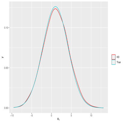
(a) True and $iid$-based density for $\theta_{1}$.

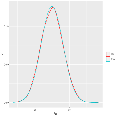
(b) True and $iid$-based density for $\theta_{25}$.

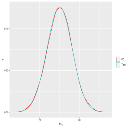
(c) True and $iid$-based density for $\theta_{75}$.

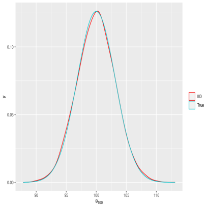
(d) True and $iid$-based density for $\theta_{100}$.

Figure 1: Simulation from $100$-dimensional normal distribution. The red and blue colours denote the $iid$ sample based density and the true density, respectively.

(a) Exact correlation structure.

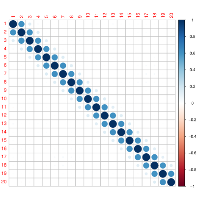
(b) Correlation structure based on $iid$ samples.

Figure 2: Simulation from $100$-dimensional normal distribution. True and $iid$-based correlation structures for the first $20$ co-ordinates.

5.2 Simulation from Student’s $t$ with $5$ degrees of freedom

In the Student’s $t$ setup, $M=1000$ turned out to be sufficient for all the dimensions that we considered; this significantly larger value of $M$ compared to that for the normal setup is due to the much thicker tails of the $t$ distribution with $5$ degrees of freedom. Depending upon the dimension, we chose the radii differently for adequate performance of our methodology. The general form of our choice is the same as in the normal setup, that is, $\sqrt{c_{1}}=r_{d}$ and $\sqrt{c_{i}}=\sqrt{c_{1}}+a_{d}\times(i-1)$, for $i=2,\ldots,M$. Following our experimentations as discussed in the normal simulation context, we set $r_{1}=5$ and $r_{d}=4$, for $d=5,10,50,100$. As regards $a_{d}$, we set $a_{1}=3.801$, $a_{5}=2.1654$, $a_{10}=2.5$, $a_{50}=0.52$ and $a_{100}=0.52$. As before, we used Monte Carlo size $N_{i}=10000$ for the construction of $\hat{\pi}(\boldsymbol{\theta})$, and then simulated $10000$ $iid$ realizations from $\hat{\pi}(\boldsymbol{\theta})$. The times taken for $d=1,5,10,50,100$ are $4$ minutes, $29$ minutes, $1$ hour $3$ minutes, less than a minute, and less than a minute, respectively. The reason for the significantly less time here compared to the normal setup is again attributable to the thick tails of the $t$ distribution; the flatter tails ensure that the infimum $s_{i}$ and supremum $S_{i}$ are not much different, entailing that $\hat{p}_{i}$ is reasonably large (see (16)), so that simulation from the geometric distribution (24) yielded significantly smaller values of the coalescence time $T_{i}$ compared to the normal setup. Thus, in spite of the larger value of $M$, these small values of $T_{i}$ led to much quicker overall computation.

Again, the $iid$ simulations turned out to be highly reliable in all the cases. Figure 3 shows the results for four co-ordinates in the context of $d=100$, and the exact and estimated correlation structures for the first $20$ co-ordinates are displayed in Figure 4.

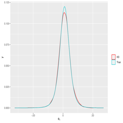
(a) True and $iid$-based density for $\theta_{1}$.

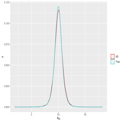
(b) True and $iid$-based density for $\theta_{25}$.

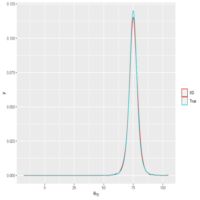
(c) True and $iid$-based density for $\theta_{75}$.

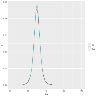
(d) True and $iid$-based density for $\theta_{100}$.

Figure 3: Simulation from $100$-dimensional Student’s $t$ distribution with $5$ degrees of freedom. The red and blue colours denote the $iid$ sample based density and the true density, respectively.

(a) Exact correlation structure.

(b) Correlation structure based on $iid$ samples.

Figure 4: Simulation from $100$-dimensional Student’s $t$ distribution with $5$ degrees of freedom. True and $iid$-based correlation structures for the first $20$ co-ordinates.

5.3 Simulation from Cauchy

In this case, we set $\sqrt{c_{1}}=r_{d}$ and $\sqrt{c_{i}}=\sqrt{c_{1}}+a_{d}\times(i-1)$, for $i=2,\ldots,M_{d}$. Thus, even the value of $M$ now depends upon $d$. Following our experimentations we obtained the following: $(r_{1}=5,a_{1}=3.801,M_{1}=2000)$, $(r_{5}=0.5,a_{5}=0.5,M_{5}=3000)$, $(r_{10}=0.5,a_{10}=0.5,M_{10}=3000)$, $(r_{50}=4,a_{50}=0.52,M_{50}=2000)$, $(r_{100}=4,a_{100}=0.52,M_{100}=2576)$. Note that the values of $M_{d}$ are at least twice that for the Student’s $t$ distribution, which is clearly due to the much thicker tail of Cauchy compared to $t$.

As before, using Monte Carlo size $N_{i}=10000$ for the construction of $\hat{\pi}(\boldsymbol{\theta})$, we then simulated $10000$ $iid$ realizations from $\hat{\pi}(\boldsymbol{\theta})$. In this case, the times taken for $d=1,5,10,50,100$ are $2$ minutes, $2$ minutes, $2$ minutes, less than a minute, and $2$ minutes, respectively. Notice the significantly less time taken in this setup compared to both normal and Cauchy. Given the thickest tail of Cauchy, the reason for this is the same as provided in Section 5.2 that explains lesser time for $t$ compared to normal.

As expected, the $iid$ simulations accurately represented the underlying Cauchy distributions. Depictions of the true and $iid$ sample based marginal densities of four co-ordinates are presented by Figure 5 in the context of $d=100$. Since the covariance structure does not exist for Cauchy, we do not present the correlation structure comparison unlike the previous cases.

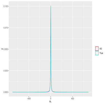
(a) True and $iid$-based density for $\theta_{1}$.

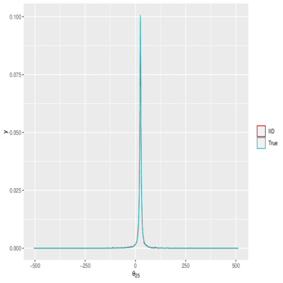
(b) True and $iid$-based density for $\theta_{25}$.

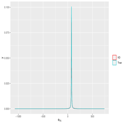
(c) True and $iid$-based density for $\theta_{75}$.

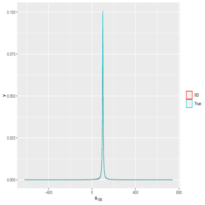
(d) True and $iid$-based density for $\theta_{100}$.

Figure 5: Simulation from $100$-dimensional Cauchy distribution. The red and blue colours denote the $iid$ sample based density and the true density, respectively.

5.4 Simulation from normal mixture

In this case, for both $\boldsymbol{A}_{1i}$ and $\boldsymbol{A}_{2i}$, we chose $r_{50}=4$ and $a_{50}=0.5$. As in the normal setup detailed in Section 5.1, $M=71$ turned out to be sufficient. We set $N_{i}=10000$ as the Monte Carlo size, as in the previous cases. For drawing each $iid$ realization, assuming known mixing probabilities $2/3$ and $1/3$, we first selected either of the two mixing densities, indexed by $j=1,2$. Then, with the corresponding sequence of sets $\boldsymbol{A}_{ji}$, we proceeded with perfect sampling from the mixing density indexed by $j$. The time taken for the entire implementation was $7$ minutes for generating $10000$ $iid$ realizations.

As before, the $iid$ realizations very accurately represented the true mixture distribution, Figure 6 bearing some testimony. Figure 7 compares the true correlation structure and that estimated by our $iid$ method. As expected, the estimated structure yielded by our $iid$ method has been highly accurate. Here it is worth remarking that the true correlation structure is also an estimated structure, based on $10000$ direct $iid$ realizations from the normal mixture.

Details of the method for generating perfect $iid$ realizations from any general multimodal target distribution $\pi$, is provided in Bhattacharya (2021).

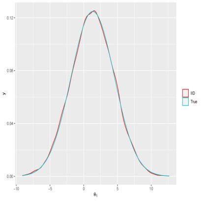
(a) True and $iid$-based density for $\theta_{1}$.

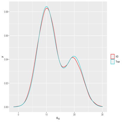
(b) True and $iid$-based density for $\theta_{10}$.

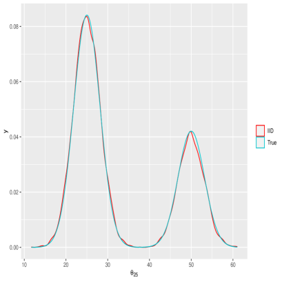
(c) True and $iid$-based density for $\theta_{25}$.

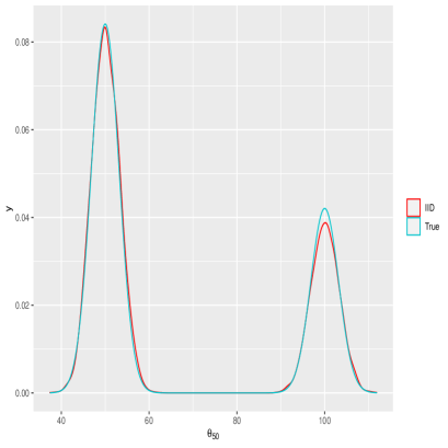
(d) True and $iid$-based density for $\theta_{50}$.

Figure 6: Simulation from $50$-dimensional mixture normal distribution. The red and blue colours denote the $iid$ sample based density and the true density, respectively.

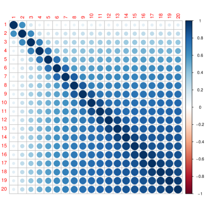
(a) Exact correlation structure.

(b) Correlation structure based on $iid$ samples.

Figure 7: Simulation from $50$-dimensional mixture normal distribution. True and $iid$-based correlation structures for the first $20$ co-ordinates.

6 Experiments with posterior distributions given real data

We now consider the application of our $iid$ method to posterior distributions given real datasets. Our first application in this regard will be the well-known Challenger space shuttle problem (see, for example, Dalal et al. (1989), Martz and Zimmer (1992) and Robert and Casella (2004), Dutta and Bhattacharya (2014)). The data can be found in Robert and Casella (2004) and in the supplement of Dutta and Bhattacharya (2014). Here we consider drawing $iid$ realizations from the two-parameter posterior distribution corresponding to a logit likelihood and compare the $iid$ based and TMCMC based posteriors.

For our second application, we shall consider the Salmonella example from Chapter 6.5.2 of Lunn et al. (2012). The data, three-parameter Poisson log-linear model, the priors and the BUGS/JAGS codes are also available at http://runjags.sourceforge.net/quickjags.html. In this example as well, we shall compare the $iid$ based and TMCMC based posteriors.

Our third application is on the really challenging, spatial data and model setup related to radionuclide count data on Rongelap Island (Diggle et al. (1997), Diggle et al. (1998)). The model for the radionuclide counts is a Poisson log-linear model encapsulating a latent Gaussian process to account for spatial dependence. The model consists of $160$ parameters. The difficulty of MCMC convergence for the posterior analysis in this problem is very well-known and several research works have been devoted to this (see, for example, Rue (2001), Christensen (2004), Christensen (2006)). Very encouragingly, even in this challenging problem, we are able to very successfully obtain $iid$ samples from the posterior, after using a specific diffeomorphic transformation to the posterior to render it sufficiently thick-tailed to yield reasonably large values of $\hat{p}_{i}$. As in the previous examples, here also we shall compare the $iid$ and TMCMC based posteriors.

6.1 Application to the Challenger dataset

In 1986, the space shuttle Challenger exploded during take off, killing the seven astronauts aboard. The explosion was the result of an O-ring failure, a splitting of a ring of rubber that seals the parts of the ship together. The accident was believed to be caused by the unusually cold weather ($31\degree$F or $0\degree$C) at the time of launch, as there is reason to believe that the O-ring failure probabilities increase as temperature decreases.

In this regard, for $i=1,\ldots,n$, where $n=23$, let $y_{i}$ denote the indicator variable denoting failure of the O-ring. Also let $x_{i}=t_{i}/\max~{}t_{i}$, where $t_{i}$ is the temperature (degrees F) at flight time $i$. We assume that for $i=1,\ldots,n$, $y_{i}\sim Bernoulli(p(x_{i}))$ independently, where $p(x_{i})=\exp(\alpha+\beta x_{i})\big{/}(1+\exp(\alpha+\beta x_{i}))$. As regards the prior for $(\alpha,\beta)$, we set $\pi(\alpha,\beta)\equiv 1$ for $\alpha,\beta\in\mathbb{R}$.

For TMCMC, we consider the additive transformation detailed in Section 4 of Dutta and Bhattacharya (2014), with scaling constants in the additive transformation being $7.944$ and $9.762$ respectively for $\alpha$ and $\beta$. After accepting the proposed additive TMCMC move or the previous state in accordance with the TMCMC acceptance probability, we conduct another mixing-enhancement step in a similar vein as in Liu and Sabatti (2000) which, given the current accepted state, proposes another move that gives either forward transformation to both the parameters or backward transformation to both the parameters, with equal probability. Either this final move, or the last accepted additive TMCMC move is accepted in accordance with the TMCMC acceptance probability. With this strategy, we run our chain for $2\times 10^{5}$ iterations, discarding the first $10^{5}$ as burn-in. We estimate $\boldsymbol{\mu}$ and $\boldsymbol{\Sigma}$ required for our sets $\boldsymbol{A}_{i}$ using the stored $10^{5}$ iterations after burn-in.

In order to select the radii, we set as before, with $d=2$, $\sqrt{c_{1}}=r_{d}$ and $\sqrt{c_{i}}=\sqrt{c_{1}}+a_{d}\times(i-1)$, for $i=2,\ldots,M$. Our experiments indicated that $M=85$, $r_{d}=2$ and $a_{d}=0.02$ are appropriate choices. Now, since $\sqrt{c_{2}}-\sqrt{c_{1}}=2\times 0.02$ and $\sqrt{c_{i}}-\sqrt{c_{i-1}}=0.02$ for $i\geq 3$, rejection sampling in order to simulate uniformly from $\boldsymbol{A}_{i}$ for $i\geq 2$ is costly computationally, since the probability of any point $\tilde{\boldsymbol{\theta}}$ drawn uniformly from the ellipsoid $\{\boldsymbol{\theta}:(\boldsymbol{\theta}-\boldsymbol{\mu})^{T}\boldsymbol{\Sigma}^{-1}(\boldsymbol{\theta}-\boldsymbol{\mu})\leq c_{i}\}$ to satisfy $(\tilde{\boldsymbol{\theta}}-\boldsymbol{\mu})^{T}\boldsymbol{\Sigma}^{-1}(\boldsymbol{\theta}-\tilde{\boldsymbol{\mu}})>c_{i-1}$, is small. To handle this, we adopt the following strategy. First observe that in this situation, $\boldsymbol{A}_{i}$ here is well approximated by the region close to the surface of the above ellipsoid. For sufficiently large value of $\tilde{d}$, $\tilde{\boldsymbol{Y}}=\sqrt{c_{i}}U^{1/\tilde{d}}\boldsymbol{X}/\|\boldsymbol{X}\|$ with $\boldsymbol{X}=(X_{1},\ldots,X_{d})^{T}$ where $X_{k}\stackrel{{\scriptstyle iid}}{{\sim}}N(0,1)$, for $k=1,\ldots,d$, $U\sim U(0,1)$, represents the uniform distribution essentially about the surface of the ball centered around $\boldsymbol{0}$ and with radius $\sqrt{c_{i}}$, so that $\tilde{\boldsymbol{\theta}}=\boldsymbol{\mu}+\boldsymbol{B}\tilde{\boldsymbol{Y}}$ essentially represents the desired uniform distribution on $\boldsymbol{A}_{i}$. Thus, this method completely avoids rejection sampling. Setting $\tilde{d}=10^{5}$ turned out to yield quite accurate results with this strategy. Indeed, comparison with actual rejection sampling showed that the final results are almost indistinguishable.

Instead of setting $N_{i}=10000$ as the Monte Carlo size as in our experiments with the standard distributions, here we set $N_{i}=5000$. One obvious reason for this is to reduce the computing time, since there are $M=10^{5}$ set $\boldsymbol{A}_{i}$ where the Monte Carlo method needs to be applied to. Another reason is that, due to the narrow regions covered individually by the current sets $\boldsymbol{A}_{i}$, not much Monte Carlo realizations are necessary. Again, we compared the results with actual rejection sampling by setting $N_{i}=10000$, and again the final results turned out to be almost the same.

There is another subtle issue that deserves mention. The above strategy for avoiding rejection sampling does not guarantee that none of the points sampled from $\boldsymbol{A}_{i}$ will fall in $\boldsymbol{A}_{i-1}$, for $i\geq 2$. Indeed, a few points must percolate into $\boldsymbol{A}_{i-1}$, but are still counted for computation of the infimum and supremum of $\tilde{\pi}(\boldsymbol{\theta})$ in $\boldsymbol{A}_{i}$. These points thus render the effect of lowering the value of the ratio of the actual infimum and supremum. To counter this effect, we set $\eta_{i}=0$ in the formula for $\hat{p}_{i}$. Note however, that the Monte Carlo estimate of $\tilde{\pi}(\boldsymbol{A}_{i})$ is unaffected by this percolation since the effect of the few points, when divided by the Monte Carlo size, is washed away.

As before, we sampled $10000$ $iid$ realizations from this Challenger posterior. The implementation time of our $iid$ method has been $22$ minutes for this problem.

Figure 8 compares the $iid$ based and TMCMC based marginal posteriors of $\alpha$ and $\beta$. Here we thinned the $10^{5}$ TMCMC realizations by using one in every $10$ for comparing with our $10000$ $iid$ realizations. Observe that the $iid$ based densities are in very close agreement with those based on TMCMC.

The TMCMC and $iid$ based posterior correlations between $\alpha$ and $\beta$ are $-0.99771$ $-0.99761$, respectively, exhibiting close agreement.

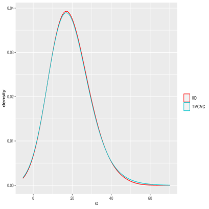
(a) TMCMC and $iid$-based density for $\alpha$.

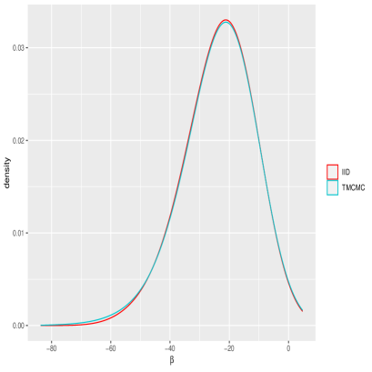
(b) TMCMC and $iid$-based density for $\beta$.

Figure 8: Challenger posterior. The red and blue colours denote the $iid$ sample based density and the TMCMC based density, respectively.

6.2 Application to the Salmonella dataset

Here the data concerned is a mutagenicity assay data on Salmonella. In the relevant experiment, three plates have each been processed at various doses of quinoline and subsequently the number of revertant colonies of TA98 Salmonella are measured; see Breslow (1984), Lunn et al. (2012).

For $i=1,\ldots,6$ and $j=1,2,3$, letting $y_{ij}$ denote the number of colonies observed on plate $j$ at dose $x_{i}$, the model considered (see Lunn et al. (2012)) is $y_{ij}\sim Poisson(\mu(x_{i}))$, where $\log(\mu_{i})=\alpha+\beta+\gamma(x_{i}+10)+\gamma x_{i}$. The priors for $\alpha,\beta,\gamma$ are independent zero-mean normal distributions with standard deviation $100$.

We first consider an additive TMCMC application to this problem, with the scaling constants in the additive transformation for $\alpha,\beta,\gamma$ being $0.21832$, $0.056563$ and $0.00024192$, respectively. The forward and backward transformations are considered with equal probability. The rest of the details remain the same as in the Challenger problem. Quite encouraging TMCMC convergence properties are indicated by our informal diagnostics. As before, $\boldsymbol{\mu}$ and $\boldsymbol{\Sigma}$ are estimated from the stored $10^{5}$ TMCMC realizations, after ignoring the first $10^{5}$ realizations as burn-in.

For application of our $iid$ method, we set, for $d=3$, $r_{d}=3$, $a_{d}=0.02$, and $M=200$, as suggested by our experiments. Again, we avoided rejection sampling in the same way as in the Challenger case, and considered $N_{i}=5000$, drawing $10000$ realizations from the three-parameter posterior. The time for implementation here is only a minute.

Figure 9 compares TMCMC and $iid$ sampling with respect to density estimation of the parameters with $10^{5}$ TMCMC realizations thinned to $10000$ realizations by considering one in every $10$. Once again, the $iid$ results are in close agreement with the TMCMC results.

The estimated correlation structures, however, are not much different with respect to the competing methods. The TMCMC estimates of the posterior correlations between $(\alpha,\beta)$, $(\alpha,\gamma)$ and $(\beta,\gamma)$ are $-0.9627896$, $0.7810736$ and $-0.8901597$, respectively, while the respective $iid$ estimates are $-0.9625148$, $0.7774780$ and $-0.8887078$.

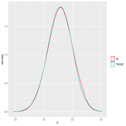
(a) TMCMC and $iid$-based density for $\alpha$.

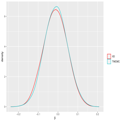
(b) TMCMC and $iid$-based density for $\beta$.

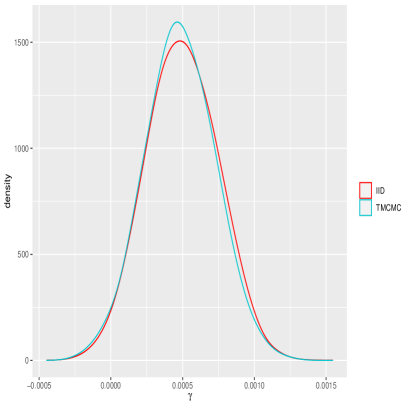
(c) TMCMC and $iid$-based density for $\gamma$.

Figure 9: Salmonella posterior. The red and blue colours denote the $iid$ sample based density and the TMCMC based density, respectively.

6.3 Application to the Rongelap Island dataset

We now consider application of our $iid$ sampling idea to the challenging spatial statistics problem involving radionuclide count data on Rongelap Island. Following Diggle et al. (1998), we model the count data, for $i=1,\ldots,157$, as

$$Y_{i}\sim Poisson(\mu_{i}),$$

where

$$\mu_{i}=t_{i}\exp\{\beta+S(\boldsymbol{x}_{i})\},$$

$t_{i}$ being the duration of observation at location $\boldsymbol{x}_{i}$, $\beta$ is an unknown parameter and $S(\cdot)$ is a zero-mean Gaussian process with isotropic covariance function of the form

$$Cov\left(S(\tilde{\boldsymbol{x}}_{1}),S(\tilde{\boldsymbol{x}}_{2})\right)=\sigma^{2}\exp\{-\alpha\parallel\tilde{\boldsymbol{x}}_{1}-\tilde{\boldsymbol{x}}_{2}\parallel\}$$

for any two locations $\tilde{\boldsymbol{x}}_{1},\tilde{\boldsymbol{x}}_{2}$. In the above, $(\sigma^{2},\alpha)$ are unknown parameters. We assume uniform priors on the entire parameter space corresponding to $(\beta,\log(\sigma^{2}),\log(\alpha))$. Since there are $157$ latent Gaussian variables $S(\boldsymbol{x}_{i})$ and three other unknowns $(\alpha,\beta,\sigma^{2})$, there are in all $160$ unknowns in this problem.

To first consider a TMCMC implementation, we adopted the same additive TMCMC sampler of Dey and Bhattacharya (2017) specific to this spatial count data problem (see Section 8 of their article), but also enhanced its convergence properties by adding the step with the flavour of Liu and Sabatti (2000) in the same way as in the previous applications regarding Challenger and Salmonella. After discarding the first $10^{6}$ realizations as burn-in, we stored one in $100$ in the next $10^{6}$ iterations, to obtain $10000$ realizations, which we used for estimation of $\boldsymbol{\mu}$ and $\boldsymbol{\Sigma}$ needed for $\boldsymbol{A}_{i}$ of our $iid$ sampler. The TMCMC exercise took about $1$ hour $40$ minutes.

Now, with $d=160$, application of the $iid$ method requires appropriate specification of $r_{d}$ and $a_{d}$ such that $\hat{p}_{i}$ are sufficiently large. However, in this challenging application, all our experiments failed to yield significant $\hat{p}_{i}$. To handle this challenge, we decided to flatten the posterior distribution in a way that its infimum and the supremum are reasonably close (so that $\hat{p}_{i}$ are adequately large) on all the $\boldsymbol{A}_{i}$. This requires an appropriate flattening bijective transformation. As it turns out, the MCMC literature already contains instances of such transformations with stronger properties such that the transformation and its inverse are continuously differentiable. Such transformations are called diffeomorphisms. In fact, diffeomorphisms with stronger properties have been considered in Johnson and Geyer (2012); see also Dey and Bhattacharya (2016) who implement such diffeomorphisms in the TMCMC context. However, in the above works, the transformations are meant to reduce thick-tailed target distributions to thin-tailed ones. Here we need just the opposite; the Rongelap Island posterior needs to be converted to a thick-tailed distribution for our $iid$ sampling purpose. As can be anticipated, the inverse transformations for thick to thin tail conversions will be appropriate here. Details follow.

6.3.1 A suitable diffeomorphic transformation and the related method

Observe that if $\pi_{\boldsymbol{\theta}}$, the multivariate target density of some random vector $\boldsymbol{\theta}$ is interest, then

$$\pi_{\boldsymbol{\gamma}}(\boldsymbol{\gamma})=\pi_{\boldsymbol{\theta}}\left(h(\boldsymbol{\gamma})\right)\left|\mbox{det}~{}\nabla h(\boldsymbol{\gamma})\right|$$ (25)

is the density of $\boldsymbol{\gamma}=h^{-1}(\boldsymbol{\theta})$, where $h$ is a diffeomorphism. In the above, $\nabla h(\boldsymbol{\gamma})$ denotes the gradient of $h$ at $\boldsymbol{\gamma}$ and $\mbox{det}~{}\nabla h(\boldsymbol{\gamma})$ stands for the determinant of the gradient of $h$ at $\boldsymbol{\gamma}$.

Johnson and Geyer (2012) obtain conditions on $h$ which make $\pi_{\boldsymbol{\gamma}}$ super-exponentially light. Specifically, they define the following isotropic function $h:\mathbb{R}^{d}\mapsto\mathbb{R}^{d}$:

$$h(\boldsymbol{\gamma})=\left\{\begin{array}[]{cc}f(\|\boldsymbol{\gamma}\|)\frac{\boldsymbol{\gamma}}{\|\boldsymbol{\gamma}\|},&\boldsymbol{\gamma}\neq\boldsymbol{0}\\ 0,&\boldsymbol{\gamma}=\boldsymbol{0},\end{array}\right.$$ (26)

for some function $f:(0,\infty)\mapsto(0,\infty)$. Johnson and Geyer (2012) confine attention to isotropic diffeomorphisms, that is, functions of the form $h$ where both $h$ and $h^{-1}$ are continuously differentiable, with the further property that $\mbox{det}~{}\nabla h$ and $\mbox{det}~{}\nabla h^{-1}$ are also continuously differentiable. In particular, if $\pi_{\boldsymbol{\beta}}$ is only sub-exponentially light, then the following form of $f:[0,\infty)\mapsto[0,\infty)$ given by

$$f(x)=\left\{\begin{array}[]{cc}e^{bx}-\frac{e}{3},&x>\frac{1}{b}\\ x^{3}\frac{b^{3}e}{6}+x\frac{be}{2},&x\leq\frac{1}{b},\end{array}\right.$$ (27)

where $b>0$, ensures that the transformed density $\pi_{\boldsymbol{\gamma}}$ of the form (25), is super-exponentially light.

In our current context, the $d=160$ dimensional target distribution $\pi_{\boldsymbol{\theta}}$ needs to be converted to some thick-tailed distribution $\pi_{\boldsymbol{\gamma}}$. Hence, we apply the transformation $\boldsymbol{\gamma}=h(\boldsymbol{\theta})$, the inverse of the transformation considered in Johnson and Geyer (2012). Consequently, the density of $\boldsymbol{\gamma}$ here becomes

$$\pi_{\boldsymbol{\gamma}}(\boldsymbol{\gamma})=\pi_{\boldsymbol{\theta}}\left(h^{-1}(\boldsymbol{\gamma})\right)\left|\mbox{det}~{}\nabla h(\boldsymbol{\gamma})\right|^{-1},$$ (28)

where $h$ is the same as (26) and $f$ is given by (27). We also give the same transformation to the uniform proposal density (15), so that the new proposal density now becomes

$$q_{i}(\boldsymbol{\gamma}^{\prime})=\frac{1}{\mathcal{L}(\boldsymbol{A}_{i})}I_{\boldsymbol{A}_{i}}(h^{-1}(\boldsymbol{\gamma}^{\prime}))\left|\mbox{det}~{}\nabla h(\boldsymbol{\gamma}^{\prime})\right|^{-1}.$$ (29)

With (29) as the proposal density for (28), the proposal will not cancel in the acceptance ratio of the Metropolis-Hastings acceptance probability. For any set $\boldsymbol{A}$, let $h(\boldsymbol{A})=\left\{h(\boldsymbol{\theta}):\boldsymbol{\theta}\in\boldsymbol{A}\right\}$. Also, now let $s_{i}=\underset{\boldsymbol{\gamma}\in h(\boldsymbol{A}_{i})}{\inf}~{}\frac{\tilde{\pi}_{\boldsymbol{\gamma}}(\boldsymbol{\gamma})}{q_{i}(\boldsymbol{\gamma})}$ and $S_{i}=\underset{\boldsymbol{\gamma}\in h(\boldsymbol{A}_{i})}{\sup}~{}\frac{\tilde{\pi}_{\boldsymbol{\gamma}}(\boldsymbol{\gamma})}{q_{i}(\boldsymbol{\gamma})}$, where $\tilde{\pi}_{\boldsymbol{\gamma}}(\boldsymbol{\gamma})$ is the same as (28) but without the normalizing constant. Then, with (29) as the proposal density we have

$$P_{i}(\boldsymbol{\gamma},h(\mathbb{B}\cap\boldsymbol{A}_{i})) \geq\int_{h(\mathbb{B}\cap\boldsymbol{A}_{i})}\min\left\{1,\frac{\tilde{\pi}_{\boldsymbol{\gamma}}(\boldsymbol{\gamma}^{\prime})/q_{i}(\boldsymbol{\gamma}^{\prime})}{\tilde{\pi}_{\boldsymbol{\gamma}}(\boldsymbol{\gamma})/q_{i}(\boldsymbol{\gamma})}\right\}q_{i}(\boldsymbol{\gamma}^{\prime})d\boldsymbol{\gamma}^{\prime}$$

$$\geq p_{i}~{}Q_{i}(h(\mathbb{B}\cap\boldsymbol{A}_{i})),$$

where $p_{i}=s_{i}/S_{i}$ and $Q_{i}$ is the probability measure corresponding to (29). The rest of the details remain the same as before with necessary modifications pertaining to the new proposal density (29) and the new Metropolis-Hastings acceptance ratio with respect to (29) incorporated in the subsequent steps. Once $\boldsymbol{\gamma}$ is generated from (28) we transform it back to $\boldsymbol{\theta}$ using $\boldsymbol{\theta}=h^{-1}(\boldsymbol{\gamma})$.

6.3.2 Results with the diffeomorphic transformation

With the transformed posterior density corresponding to the form (25), our experiments suggested that $M=10000$, $b=0.01$, $r_{d}=7.8$ and $a_{d}=0.0005$ are appropriate, and rendered $\hat{p}_{i}$ significantly large for the transformed target. With $N_{i}=5000$ and the technique of avoiding rejection sampling remaining the same as in the previous two applications, generation of $10000$ $iid$ realizations took $30$ minutes in our parallel processors.

Figures 10 and 11 show that the marginal density estimates with the TMCMC based and the $iid$ based samples are in agreement, as in the previous examples. That the correlation structures obtained by both the methods are also in close agreement, is borne out by Figure 12.

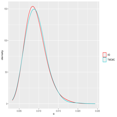
(a) TMCMC and $iid$-based density for $\alpha$.

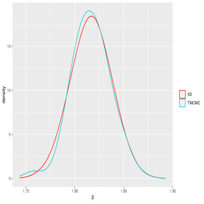
(b) TMCMC and $iid$-based density for $\beta$.

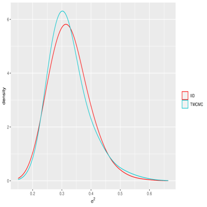
(c) TMCMC and $iid$-based density for $\sigma^{2}$.

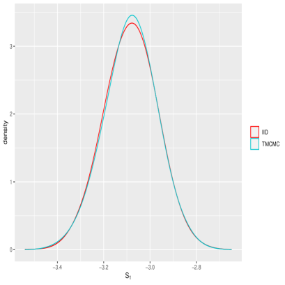
(d) TMCMC and $iid$-based density for $S_{1}$.

Figure 10: Rongelap Island posterior. The red and blue colours denote the $iid$ sample based density and the TMCMC based density, respectively.

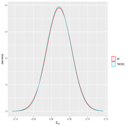
(a) TMCMC and $iid$-based density for $S_{10}$.

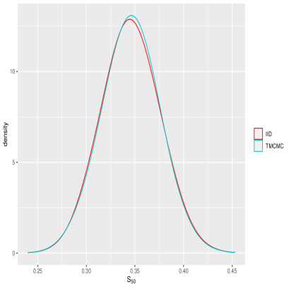
(b) TMCMC and $iid$-based density for $S_{50}$.

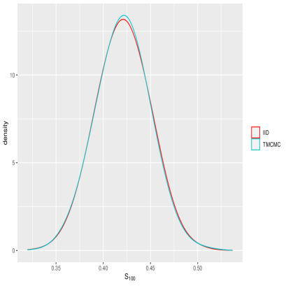
(c) TMCMC and $iid$-based density for $S_{100}$.

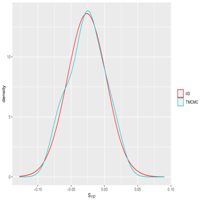
(d) TMCMC and $iid$-based density for $S_{157}$.

Figure 11: Rongelap Island posterior. The red and blue colours denote the $iid$ sample based density and the TMCMC based density, respectively.

(a) TMCMC based correlation structure.

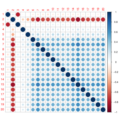
(b) Correlation structure based on $iid$ samples.

Figure 12: Rongelap Island posterior. TMCMC and $iid$-based correlation structures for the first $20$ co-ordinates.

7 Summary and conclusion

In this article, we have attempted to provide a valid and practically feasible methodology for generating $iid$ realizations from any target distribution on the Euclidean space of arbitrary dimensionality. The key insight leading to the development is that, perfect simulation, which lies at the heart of our methodology, is expected to be practically feasible if implemented on appropriately constructed compact sets on which the target density is relatively flat. This motivated us to create an infinite sequence of concentric compact ellipsoids such that the target density restricted to the central ellipsoid and the ellipsoidal annuli are expected to be amenable to very feasible perfect sampling.

We formally attempted to achieve this by representing the target distribution as an infinite mixture of such densities. Consequently, to generate a realization from the target, a mixture component can be picked with its corresponding mixing probability and a realization can be obtained exactly from the mixture component by perfect simulation. Using minorization, we achieve the goal of appropriate perfect sampler construction for the mixture densities restricted on the ellipsoids and the annuli. The computational burden of the CFTP based search method for perfect sampling is avoided in our approach by accommodating the proposed idea of Murdoch and Green (1998) with due rectification. Amalgamating the above ideas coherently enabled us to construct an efficient parallel algorithm for $iid$ sampling from general target distributions, with or without compact supports.

Applications of our $iid$ sampling algorithm to various standard univariate and multivariate distributions, with dimension as high as $100$, vindicated the accuracy and computational efficiency of our ideas. Further applications to real data scenarios again brought out the usefulness, general applicability and reliability of our method.

The particularly important and challenging real data application is that of the spatial radionuclide count data on Rongelap Island, consisting of $160$ parameters and ill-famed for rendering most MCMC approaches ineffective. In this case, using our original strategy we were initially unable to obtain any ellipsoid sequence amenable to feasible perfect sampling. However, application of an appropriate flattening diffeomorphic transformation to the posterior density seemed to be an appropriate response to the challenge, and facilitated cheap implementation of $iid$ sampling. It thus seems that the class of diffeomorphic transformations is destined to play an important role in further development of our research in this extremely important topic of $iid$ sampling from general intractable distributions.

References

- Bhattacharya (2021) Bhattacharya, S. (2021). IID Sampling from Intractable Multimodal and Variable-Dimensional Distributions. arXiv preprint.
- Breslow (1984) Breslow, N. (1984). Extra-Poisson Variation in Log-Linear Models. Applied Statistics, 33, 38–44.
- Christensen (2004) Christensen, O. F. (2004). Monte Carlo Maximum Likelihood in Model-Based Geostatistics. Journal of Computational and Graphical Statistics, 13, 702–718.
- Christensen (2006) Christensen, O. F. (2006). Robust Markov Chain Monte Carlo Methods for Spatial Generalized Linear Mixed Models. Journal of Computational and Graphical Statistics, 15, 1–17.
- Dalal et al. (1989) Dalal, S. R., Fowlkes, E. B., and Hoadley, B. (1989). Risk Analysis of the Space Shuttle: pre-Challenger Prediction of Failure. Journal of the American Statistical Association, 84, 945–957.
- Dey and Bhattacharya (2016) Dey, K. K. and Bhattacharya, S. (2016). On Geometric Ergodicity of Additive and Multiplicative Transformation Based Markov Chain Monte Carlo in High Dimensions. Brazilian Journal of Probability and Statistics, 30, 570–613. Also available at “http://arxiv.org/pdf/1312.0915.pdf”.
- Dey and Bhattacharya (2017) Dey, K. K. and Bhattacharya, S. (2017). A Brief Tutorial on Transformation Based Markov Chain Monte Carlo and Optimal Scaling of the Additive Transformation. Brazilian Journal of Probability and Statistics, 31, 569–617. Also available at “http://arxiv.org/abs/1307.1446”.
- Diggle et al. (1997) Diggle, P. J., Tawn, J. A., and Moyeed, R. A. (1997). Geostatistical Analysis of Residual Contamination from Nuclear Weapons Testing. In V. Barnet and K. F. Turkman, editors, Statistics for Environment 3: Pollution Assessment and Control, pages 89–107. Chichester: Wiley.
- Diggle et al. (1998) Diggle, P. J., Tawn, J. A., and Moyeed, R. A. (1998). Model-Based Geostatistics (with discussion). Applied Statistics, 47, 299–350.
- Dutta and Bhattacharya (2014) Dutta, S. and Bhattacharya, S. (2014). Markov Chain Monte Carlo Based on Deterministic Transformations. Statistical Methodology, 16, 100–116. Also available at http://arxiv.org/abs/1106.5850. Supplement available at http://arxiv.org/abs/1306.6684.
- Giraud (2015) Giraud, C. (2015). Introduction to High-Dimensional Statistics. CRC Press, Boca Raton, FL.
- Johnson and Geyer (2012) Johnson, L. T. and Geyer (2012). Variable Transformation to Obtain Geometric Ergodicity in the Random-Walk Metropolis Algorithm. The Annals of Statistics, 40, 3050–3076.
- Liu and Sabatti (2000) Liu, J. S. and Sabatti, S. (2000). Generalized Gibbs Sampler and Multigrid Monte Carlo for Bayesian Computation. Biometrika, 87, 353–369.
- Lunn et al. (2012) Lunn, D., Jackson, C., Best, N., Thomas, A., and Spiegelhalter, D. (2012). The BUGS Book: A Practical Introduction to Bayesian Analysis. CRC Press, Boca Raton, Florida.
- Martz and Zimmer (1992) Martz, H. F. and Zimmer, W. J. (1992). The Risk of Catastrophic Failure of the Solid Rocket Boosters on the Space Shuttle. The American Statistician, 46, 42–47.
- Mukhopadhyay and Bhattacharya (2012) Mukhopadhyay, S. and Bhattacharya, S. (2012). Perfect Simulation for Mixtures with Known and Unknown Number of Components. Bayesian Analysis, 7, 675–714.
- Murdoch and Green (1998) Murdoch, D. and Green, P. J. (1998). Exact sampling for a continuous state. Scandinavian Journal of Statistics, 25, 483–502.
- Propp and Wilson (1996) Propp, J. G. and Wilson, D. B. (1996). Exact Sampling with Coupled Markov Chains and Applications to Statistical Mechanics. Random Structures and Algorithms, 9, 223–252.
- Robert and Casella (2004) Robert, C. P. and Casella, G. (2004). Monte Carlo Statistical Methods. Springer-Verlag, New York.
- Rue (2001) Rue, H. (2001). Fast sampling of Gaussian Markov random fields. Journal of the Royal Statistical Society. Series B, 63, 325–338.