MVPipe: Enabling Lightweight Updates and Fast Convergence in Hierarchical Heavy Hitter Detection

Abstract

Finding hierarchical heavy hitters (HHHs) (i.e., hierarchical aggregates with exceptionally huge amounts of traffic) is critical to network management, yet it is often challenged by the requirements of fast packet processing, real-time and accurate detection, as well as resource efficiency. Existing HHH detection schemes either incur expensive packet updates for multiple aggregation levels in the IP address hierarchy, or need to process sufficient packets to converge to the required detection accuracy. We present MVPipe, an invertible sketch that achieves both lightweight updates and fast convergence in HHH detection. MVPipe builds on the skewness property of IP traffic to process packets via a pipeline of majority voting executions, such that most packets can be updated for only one or few aggregation levels in the IP address hierarchy. We show how MVPipe can be feasibly deployed in P4-based programmable switches subject to limited switch resources. We also theoretically analyze the accuracy and coverage properties of MVPipe. Evaluation with real-world Internet traces shows that MVPipe achieves high accuracy, high throughput, and fast convergence compared to six state-of-the-art HHH detection schemes. It also incurs low resource overhead in the Tofino switch deployment.

I Introduction

Network administrators often need to measure and characterize the anomalous behaviors of IP traffic in operational networks. IP traffic is inherently hierarchical. It can be organized in hierarchical forms in one or multiple dimensions. For example, it can be aggregated either by source IP address prefixes (i.e., one-dimensional (1D)), or by the source-destination IP address prefixes (i.e., two-dimensional (2D)). Given the hierarchical nature of IP traffic, finding hierarchical heavy hitters (HHHs) (i.e., the hierarchical aggregates with exceptionally huge amounts of traffic) is of particular interest to network measurement [12, 39, 17, 26]. One notable application of HHH detection is to identify distributed denial-of-service (DDoS) or botnet attacks [32, 15], in which the traffic aggregates of multiple attack flows can bring substantial damage to a network.

Unlike the classical heavy hitter (HH) detection problem [13, 19, 23], whose goal is to identify individual large-sized flows (i.e., HHs), HHH detection is a much more challenging task as it needs to identify not only the HHs, but also the set of flows that have small sizes each but have a huge aggregate size when combined together. As there are many possibilities for aggregating traffic at different levels in the IP address hierarchy (e.g., multiple lengths of prefixes in IP addresses), enumerating all possible combinations of traffic aggregates is infeasible for HHH detection. This motivates the need for specialized algorithmic designs for HHH detection.

Like most network measurement tasks, practical HHH detection schemes need to address the challenges of managing the ever-increasing speed and size of IP traffic in modern networks. For a typical backbone link with a bandwidth of tens or hundreds of Gigabits per second, network measurement tasks should efficiently track millions of concurrently active flows at any time. Maintaining per-flow states, or even any combination of traffic aggregates in HHH detection, inevitably has tremendous resource demands. In addition, with the emergence of programmable networking, new network measurement solutions (e.g., [34, 16, 27]) often offload packet processing to programmable hardware switches for scalable network measurement. Unfortunately, the available switch resources are scarce (e.g., less than 2 MB of SRAM per processing stage [6, 34]), thereby complicating the use of HHH detection in programmable hardware switches. To this end, HHH detection should aim for the following design requirements: (i) fast packet processing (i.e., keeping pace with the line rate of operational networks), (ii) real-time and accurate detection (i.e., identify all HHHs in real-time with low false positive/negative rates), and (iii) resource efficiency (i.e., the computational and memory resources should be limited within their available capacities in both hardware and software).

HHH detection has been extensively studied in the literature for more than a decade (see §VII for details). One class of HHH detection schemes is streaming-based [21, 11, 24, 39, 37, 25], in which they use memory-efficient stream data structures to process IP traffic and detect HHHs at short time scales, at the expense of incurring bounded errors on detection. However, such schemes often have high processing costs to capture multiple aggregation levels of HHHs in stream data structures, and hence cannot be readily scaled to line-rate processing in modern networks. Another class of HHH detection schemes is sampling-based, by updating a sketch instance with only a sampled subset of packets [3, 2]. One representative example is randomized HHH (RHHH) [3], which detects HHHs at long time scales. RHHH maintains multiple instances of sketches for different aggregation levels and randomly selects one instance to update per packet. It has high update performance, but has slow convergence, as the HHHs cannot be detected until sufficient packets have been processed. Furthermore, both streaming-based and sampling-based HHH detection schemes have been deployed in hardware [17, 26, 30, 20, 2], but their designs often face different limitations, such as relying on a controller to specify what HHHs are monitored [17, 26], requiring specialized hardware (e.g., TCAM) to maintain high update throughput [30, 20], or sampling packets to trade convergence for resource efficiency in hardware [2].

We present MVPipe, an invertible sketch that achieves lightweight updates, fast convergence, and resource efficiency in HHH detection, in both software and hardware. By “invertible”, we mean that MVPipe can directly return all HHHs (with high accuracy) from the data structure itself. MVPipe’s design builds on the observation that IP traffic is highly skewed across multiple aggregation levels, in which most IP traffic belonging to large flows can be aggregated in a single level, while only a small fraction of traffic needs to be aggregated across all levels in the IP address hierarchy. Specifically, MVPipe maintains its sketch with small and static memory allocation (i.e., the memory can be pre-allocated a priori) and tracks aggregates via the pipelined executions of the majority vote algorithm (MJRTY) [7]. For most packets, MVPipe only updates a single level with a single MJRTY execution, while only for a small fraction of packets, MVPipe needs to update more levels along the pipeline with multiple MJRTY executions (i.e., lightweight updates). In addition, MVPipe processes all packets within its sketch, so it can detect HHHs at short time scales (i.e., fast convergence) as opposed to sampling-based approaches. Furthermore, with small and static memory allocation, MVPipe can be readily deployed in programmable hardware switches.

While we motivate our HHH detection problem from the hierarchical nature of IP traffic, we expect that our MVPipe design is also applicable to general types of hierarchical datasets, such as geographic or temporal datasets [24].

The contributions of this paper are summarized as follows.

• We design MVPipe, a novel invertible sketch for HHH detection with three major design features: lightweight updates, fast convergence, and resource efficiency for deployment in both software and hardware.

• We implement MVPipe on P4-based programmable switches [28] and compile our prototype in the Tofino chipset [36], subject to limited hardware resources.

• We conduct theoretical analysis on MVPipe, including its space and time complexities, accuracy, and coverage.

• We conduct trace-driven evaluation on MVPipe in both software and hardware. Evaluation in software shows that MVPipe achieves higher detection accuracy, faster convergence, and up to $22.13\times$ throughput gain compared to six state-of-the-art HHH detection schemes. MVPipe also incurs limited resource overhead in the Tofino switch deployment.

We open-source our MVPipe prototype in both software and P4 at https://github.com/Grace-TL/MVPipe.

II Problem Formulation

We formulate the HHH detection problem; similar formulations are also found in [11, 24, 3]. We focus on IP traffic, which can be aggregated by different prefixes in the IP address space. We model IP traffic as a stream of packets. Each packet is denoted by a tuple $(f,v_{f})$ and is allowed to be processed only once. In network measurement, $f$ identifies a flow, and $v_{f}$ is either one (for packet counting) or the packet size (for byte counting). In this work, we consider one-dimensional (1D) and two-dimensional (2D) HHH detection: for 1D HHH detection, $f$ refers to a source IP address (the same arguments hold for a destination IP address); for 2D HHH detection, $f$ refers to a source-destination IP address pair.

We aggregate source addresses or source-destination address pairs by the address prefixes at either byte-level or bit-level granularities; we refer to them as 1D-byte, 2D-byte, 1D-bit, and 2D-bit hierarchies. Figure 1 shows the 1D-byte and 2D-byte hierarchies. Each node corresponds to the key of a flow at a certain aggregation level in a hierarchy. We define the level of a node as the position in a hierarchy of depth $d$, where the level ranges between 0 and $d-1$. The key at the lowest level 0 is the most specific and refers to an exact address (1D) or an address pair (2D), while the key at the highest level $d-1$ corresponds to the most general aggregate (i.e., all addresses or address pairs). In general, a key refers to an address prefix (1D) or a pair of address prefixes (2D). The keys of lower-level nodes (a.k.a. descendants) can be generalized to the keys of their higher-level nodes (a.k.a. ancestors); for example, the key $1.2.3.4$ can be generalized by one byte to $1.2.3.*$. Let $\prec$ be the generalization relation of two keys. For any keys $x$ and $y$, we say that $x\prec y$ if $x$ can be generalized to $y$, and that $x\preceq y$ if $x\prec y$ or $x=y$.

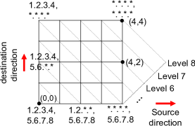
(a) 1D-byte hierarchy	(b) 2D-byte hierarchy

Figure 1: 1D-byte and 2D-byte hierarchies.

To quantify the level of a node, we associate each node with a coordinate in multi-dimensional space as shown in Figure 1. The $i$-th element of the coordinate represents the degree of generalization in the $i$-th dimension. Then the level of a node is the sum of all elements of the node’s coordinate. For example, in Figure 1(a), the node with coordinate $(1)$ is at level 1; in Figure 1(b), the node with coordinate $(4,2)$ is at level 6. In multi-dimensional space, multiple nodes can reside at the same level (e.g., see the 2D case in Figure 1(b)). We denote the set of nodes at level $i$ by $\mathcal{L}(i)$.

We now formally define HHHs. Let $S(x)=\sum_{f\preceq x}S(f)$ be the count of a key $x$ (i.e., packet count or byte count), where $S(f)$ denotes the sum of all $v_{f}$’s for every flow $f$ under $x$; for example, if $x$ refers to a subnet, $S(x)$ is the total count of all flows under the subnet. Intuitively, a key $x$ is an HHH if $S(x)$ exceeds some pre-defined threshold. However, if the count of a key exceeds a threshold, so do the counts of all its ancestors, which cover the key itself. To concisely define HHHs, we focus on the conditioned count of a key [24, 3], defined as the total count of all its associated flows that do not belong to any HHH. Specifically, for a key $x$ and a set of HHHs $\mathcal{H}$, the conditioned count of $x$ with respect to $\mathcal{H}$ is $S_{\mathcal{H}}(x)=\sum S(f):(f\preceq x)\wedge(\nexists y\in\mathcal{H},$ where $f\preceq y)$. Thus, we can formally define an HHH in an inductive fashion:

Definition 1.

(Hierarchical heavy hitters (HHHs) [11]). Let $\mathcal{S}$ be the total count of all flows and $\phi$ be a fractional threshold (where $0<\phi<1$). We define $\mathcal{H}_{i}$ as the set of HHHs at level $i$ (where $0\leq i<d$), such that:

• $\mathcal{H}_{0}$ is a set of flows, in which each flow $f$ has count $S(f)\geq\phi\mathcal{S}$ (i.e., $f$ is a heavy hitter);

• $\mathcal{H}_{i}=\mathcal{H}_{i-1}\cup\{x:(x\in\mathcal{L}(i))\wedge(S_{\mathcal{H}_{i-1}}(x)\geq\phi\mathcal{S})\}$; and

• $\mathcal{H}_{d-1}$ is the set of all HHHs.

We perform HHH detection at fixed-time intervals called epochs. Our goal is to find: (i) the set of all HHHs (whose conditioned counts exceed $\phi\mathcal{S}$) at the end of each epoch and (ii) the count $S(x)$ of each key $x$ that is identified as an HHH.

III MVPipe Design

MVPipe is a novel invertible sketch for HHH detection, with three major design goals: lightweight updates, fast convergence, and resource efficiency.

MVPipe builds on the skewness of IP traffic to find HHHs. Field studies [14, 38, 31] show that IP traffic is highly skewed, in which a small fraction of flows accounts for a majority of traffic. We argue that the skewness property also holds across aggregation levels. To justify, we evaluate the real-world IP traffic traces from CAIDA [8] (see §VI-A for details) on the cumulative percentage of packet counts versus the top percentage of keys at different aggregation levels. Figure 2 plots the results for the 1D-byte and 2D-byte hierarchies for some aggregation levels in IPv4 traffic. We observe that the top-10% of keys at each level all account for more than 65% of IP traffic at that level.

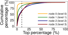
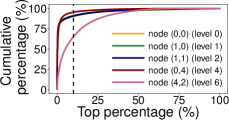
(a) 1D-byte hierarchy	(b) 2D-byte hierarchy

Figure 2: Cumulative percentage of packet counts versus the top-percentage of keys at different aggregation levels. The dashed line denotes the top-10% mark. Here, we focus on IPv4 traffic.

MVPipe tracks the candidate HHHs that are likely the true HHHs via the pipelined executions of the majority vote algorithm (MJRTY) [7]. MJRTY is a one-pass, constant-memory algorithm that finds the item that has more than half of the occurrences (i.e., the majority item) in a data stream. It is proven that if the majority item exists, MJRTY can always find the majority item [7].

Based on MJRTY, MVPipe maintains an array of buckets for each node in a hierarchy. Each bucket performs MJRTY to find the dominant key among all packets that are hashed to the bucket itself (i.e., the majority item in MJRTY) as the candidate HHH for the bucket. Then MVPipe processes each packet $(f,v_{f})$ starting from the lowest level 0 (i.e., node (0) in the 1D hierarchy or node (0,0) in the 2D hierarchy) in the hierarchy. If $f$ does not belong to any candidate HHH at a lower level, MVPipe generalizes $f$ to its ancestor at the next higher level and checks if the ancestor is a candidate HHH at that level. MVPipe proceeds toward higher levels, until $f$ is admitted by a candidate HHH (i.e., the value $v_{f}$ is included in the count of the candidate HHH).

We justify how MVPipe achieves its design goals:

• Lightweight updates: By the skewness of IP traffic, the pipelined design of MVPipe stops processing most of the packets at lower-level arrays and passes only a small fraction of packets to higher-level arrays. Also, the processing of each packet in each array of MVPipe only contains one hash computation and one memory access. Thus, the amortized processing cost is low.

• Fast convergence: MVPipe processes every packet (without sampling) in the same data structure and ensures that any HHH can be detected with high accuracy at short time scales.

• Resource efficiency: MVPipe requires only primitive computations in packet processing (e.g., hashing, addition, and subtraction). Also, MVPipe supports static memory allocation (i.e., its memory space can be pre-allocated in advance) and incurs limited memory usage. Such features allow MVPipe to be readily implemented in both hardware and software (§IV).

III-A Data Structure

Figure 3 shows the data structure of MVPipe. It comprises $H$ arrays, denoted by $A_{0},A_{1},\cdots,A_{H-1}$, where $H$ is the number of nodes in the hierarchy. Each array $A_{i}$ (where $0\leq i<H$) contains $w_{i}$ buckets and corresponds to one node in the hierarchy. Let $B(i,j)$ be the $j$-th bucket in array $A_{i}$, where $0\leq j<w_{i}$. Each bucket $B(i,j)$ consists of four fields: (i) $K_{i,j}$, which stores the candidate HHH in the bucket; (ii) $V_{i,j}$, which is the total count of all keys hashed to the bucket; (iii) $I_{i,j}$, which is the indicator counter that checks if the current candidate HHH in $K_{i,j}$ should be kept or replaced by MJRTY; and (iv) $C_{i,j}$, which is the cumulative count of the candidate HHH since it is stored in $K_{i,j}$. MVPipe is associated with $H$ pairwise-independent hash functions $h_{0},h_{1}\cdots h_{H-1}$, such that each $h_{i}$ (where $0\leq i<H$) hashes the generalization of the key of each incoming packet to one of the $w_{i}$ buckets in $A_{i}$.

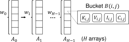
Figure 3: Data structure of MVPipe. Each bucket $B(i,j)$ (where $0\leq i<H$ and $0\leq j<w_{i}$) has four fields: $K_{i,j}$, $V_{i,j}$, $I_{i,j}$, and $C_{i,j}$.

MVPipe currently associates a single array with each node in the hierarchy. It can improve the HHH detection accuracy by associating multiple arrays with each node in the hierarchy, at the expense of degraded update performance. We discuss the trade-off in §V-B.

III-B 1D HHH Detection

We first consider the operations of MVPipe in 1D HHH detection, whose pseudo-code is shown in Figure 4. MVPipe supports two major operations: (i) Update, which updates each packet $(f,v_{f})$ into the data structure; and (ii) Detect, which returns the set of all HHHs and their respective estimated counts from the data structure. It also builds on two functions: (i) Push, which pushes the updates of a key and its corresponding count along the arrays; and (ii) Estimate, which returns an estimated count of a key in its hashed bucket. Note that in 1D HHH detection, each node in a hierarchy corresponds to a distinct level. Thus, each array $A_{i}$ corresponds to level $i$, where $0\leq i<H$.

1:function Push(key, value, $l$)

2:    $(x,v_{x})\leftarrow(\textrm{key},\textrm{value})$

3:    for $i=l$ to $H-1$ do

4:         $x\leftarrow$ generalize $x$ at level $i$

5:         $V_{i,h_{i}(x)}\leftarrow V_{i,h_{i}(x)}+v_{x}$

6:         if $K_{i,h_{i}(x)}=x$ then

7:             $I_{i,h_{i}(x)}\leftarrow I_{i,h_{i}(x)}+v_{x}$

8:             $C_{i,h_{i}(x)}\leftarrow C_{i,h_{i}(x)}+v_{x}$

9:             return

10:         else if $I_{i,h_{i}(x)}\geq v_{x}$ then

11:             $I_{i,h_{i}(x)}\leftarrow I_{i,h_{i}(x)}-v_{x}$

12:         else$\triangleright$ $K_{i,h_{i}(x)}\neq x$ and $I_{i,h_{i}(x)}<v_{x}$

13:             $I_{i,h_{i}(x)}\leftarrow v_{x}-I_{i,h_{i}(x)}$

14:             swap $(K_{i,h_{i}(x)},C_{i,h_{i}(x)})$ and $(x,v_{x})$              

15:function Estimate($x$, $l$, $t$)

16:    $U_{l}\leftarrow(V_{l,h_{l}(x)}+I_{l,h_{l}(x)})/2$

17:    $v\leftarrow C_{l,h_{l}(x)}$

18:    for $i=l+1$ to $\min\{l+t,H-1\}$ do

19:         $y\leftarrow$ generalize $x$ at level $i$

20:         if $K_{i,h_{i}(y)}$ = $y$ then

21:             $U_{i}=(V_{i,h_{i}(y)}+I_{i,h_{i}(y)})/2+v$

22:             $v\leftarrow v+C_{i,h_{i}(y)}$

23:         else

24:             $U_{i}=(V_{i,h_{i}(y)}-I_{i,h_{i}(y)})/2+v$              

25:    return $\min_{l\leq i\leq\min\{l+t,H-1\}}\{U_{i}\}$

26:procedure Update($f,v_{f}$)

27:    Push($f,v_{f},0$)

28:procedure Detect

29:    $\mathcal{A},\mathcal{H}_{o},\mathcal{H}_{1},\dots,\mathcal{H}_{H-1}\leftarrow\emptyset$

30:    for $i=0$ to $H-1$ do

31:         for $j=0$ to $w_{i}-1$ do

32:             $x\leftarrow K_{i,j}$

33:             $\hat{S}_{\mathcal{H}_{i-1}}(x)\leftarrow$ Estimate($x$, $i$, $t$) $\triangleright$ $\mathcal{H}_{i-1}=\emptyset$ for $i=0$

34:             if $\hat{S}_{\mathcal{H}_{i-1}}(x)>\phi\mathcal{S}$ then

35:                 $\hat{S}(x)\leftarrow\hat{S}_{\mathcal{H}_{i-1}}(x)+\sum_{x^{\prime}\in\mathcal{H}_{i-1}\wedge x^{\prime}\prec x}C_{i^{\prime},h_{i^{\prime}}(x^{\prime})}$ $\triangleright$ $i^{\prime}$ is the level of $x^{\prime}$

36:                 $\mathcal{A}\leftarrow\mathcal{A}\cup{(x,\hat{S}(x))}$

37:             else

38:                 Push($x,V_{i,j},i+1$)                       

39:         $\mathcal{H}_{i}\leftarrow\mathcal{H}_{i-1}\cup\mathcal{A}$

40:         $\mathcal{A}\leftarrow\emptyset$     

41:    return $\mathcal{H}_{H-1}$

Figure 4: Major operations for 1D HHH detection.

Update operation.

We apply the Update operation to insert each incoming packet to MVPipe, starting from $A_{0}$. At a high level, we hash the flow key of each packet to one of the buckets in $A_{0}$ and check if the flow key is a candidate HHH in the bucket via MJRTY. If so, we end the update; otherwise, we generalize the flow key to its ancestor at the next higher level 1 and continue to insert the ancestor to $A_{1}$. We update $A_{1}$ and the remaining arrays in a similar way until the flow key is admitted by a candidate HHH. During the process, if the original candidate HHH stored in MVPipe is replaced by the current generalized flow key due to MJRTY, we generalize the original candidate HHH and insert it into higher-level arrays.

We elaborate on the Update operation (Lines 26-27 of Figure 4) as follows. At the beginning of each epoch, we initialize the counters of all buckets of MVPipe to zeros. We update each incoming packet $(f,v_{f})$ starting from array $A_{0}$ of MVPipe by calling the Push($f,v_{f},0$) function, which processes $f$ starting from level 0 until $f$ is admitted by a candidate HHH in one of the levels.

The Push function (Lines 1-14 of Figure 4) takes a key, its associated value, and the array index $l$ (where $0\leq l<H$) as input. We first initialize $(x,v_{x})$ from the input, where $(x,v_{x})$ is passed along the arrays at higher levels (Line 2). For each array $A_{i}$ (where $l\leq i<H$), we generalize $x$ at level $i$ (Line 4) and hash the new $x$ into the bucket $B(i,h_{i}(x))$. We increment $V_{i,h_{i}(x)}$ by $v_{x}$ and check if $x$ should become the candidate HHH of the bucket based on MJRTY. Specifically, if $K_{i,h_{i}(x)}$ equals $x$ (i.e., $x$ is already a candidate HHH), we increment both $I_{i,h_{i}(x)}$ and $C_{i,h_{i}(x)}$ by $v_{x}$ and return (Lines 6-9); else if $x$ is not the candidate HHH and $I_{i,h_{i}(x)}$ is at least $v_{x}$, we decrement $I_{i,h_{i}(x)}$ by $v_{x}$ (Lines 10-11); otherwise, if $x$ is not the candidate HHH and $I_{i,h_{i}(x)}$ is below $v_{x}$, it means that $x$ should now become the new candidate HHH in $B(i,j)$. Then we should update $K_{i,h_{i}(x)}$ and $C_{i,h_{i}(x)}$ with $x$ and $v_{x}$, respectively, and aggregate the count of the original key in $K_{i,h_{i}(x)}$ to the next higher level. More precisely, we set $I_{i,h_{i}(x)}$ to $v_{x}-I_{i,h_{i}(x)}$ and swap $(K_{i,h_{i}(x)},C_{i,h_{i}(x)})$ and $(x,v_{x})$ (Lines 12-14).

From the Update operation, it is clear that once the candidate HHH is stored in $K_{i,j}$, its subsequent values received at level $i$ (i.e. $C_{i,j}$) are not pushed to higher levels. In other words, the cumulative count of a candidate HHH is not aggregated to any of its ancestors at higher levels.

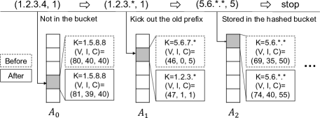
Figure 5: Example of the Update operation in MVPipe.

Example. Figure 5 depicts the Update operation. Suppose that a packet $(f,v_{f})=(1.2.3.4,1)$ arrives. If, say, 1.2.3.4 is not the candidate HHH in the hashed bucket in $A_{0}$ and the branch in Lines 10-11 holds, we generalize 1.2.3.4 into 1.2.3.* and proceed to the next level. If, say, 1.2.3.* is not the candidate HHH in the hashed bucket in $A_{1}$ but the branch in Line 12-14 holds (i.e., it now becomes the candidate HHH), we substitute the original candidate HHH 5.6.7.* by 1.2.3.*. We now generalize 5.6.7.* into 5.6.*.* and push (5.6.*.*, 5) to the next level. If, say, 5.6.*.* is the candidate HHH in $A_{2}$ (i.e., the branch in Lines 6-9 holds), the Update operation updates the counters and terminates (i.e., $f$ is now admitted by 5.6.*.*).

Detect operation.

We apply the Detect operation at the end of each epoch to find all HHHs and their estimated counts. At a high level, we traverse all arrays of MVPipe and check if the candidate HHH in each bucket should be reported as an HHH. We start from the array $A_{0}$ and check each candidate HHH: if the estimated conditioned count of the candidate HHH exceeds the threshold, we treat the candidate HHH as an HHH and include both the candidate HHH and its estimated count into the output set $\mathcal{H}_{H-1}$; otherwise, the candidate HHH should not be reported as an HHH and its key and cumulative count should be further pushed to higher-level arrays (as one of its ancestors may be reported as an HHH).

We elaborate on the Detect operation (Lines 28-41 of Figure 4) as follows. Let $\hat{S}_{\mathcal{H}_{i-1}}(x)$ and $\hat{S}(x)$ be the estimated conditioned count at level $i$ and the estimated count of key $x$, respectively. For each bucket $B(i,j)$ (where $0\leq i<H$ and $0\leq j<w_{i}$), we call the Estimate function to return the estimated conditioned count $\hat{S}_{\mathcal{H}_{i-1}}(x)$ of key $x$ stored in $K_{i,j}$ (Lines 32-33). If $\hat{S}_{\mathcal{H}_{i-1}}(x)$ exceeds the threshold $\phi\mathcal{S}$, we further calculate the estimated count $\hat{S}(x)$ and add $x$ to $\mathcal{A}$, where $\mathcal{A}$ is the set of detected HHHs at level $i$ (Lines 34-36). Otherwise, we call the Push function to push ($x,C_{i,j}$) to the next higher level $i+1$ (Lines 37-38). After processing array $A_{i}$, we update $\mathcal{H}_{i}$ as the union of $\mathcal{H}_{i-1}$ and $\mathcal{A}$, and reset $\mathcal{A}$ to empty (Line 39-40).

For each reported HHH $x$ at level $i$, we need to calculate its estimated count $\hat{S}(x)$. From the Update operation, we note that the cumulative count of each of $x$’s descendants that are reported as HHHs in $\mathcal{H}_{i-1}$ is not pushed to the hashed bucket of $x$. Thus, we need to include such “missing” counts in the calculation of $\hat{S}(x)$. We calculate $\hat{S}(x)$ as the sum of: (i) the estimated conditioned count $\hat{S}_{\mathcal{H}_{i-1}}(x)$ is returned by the Estimate function (see details below) and (ii) the cumulative counts of $x$’s descendants that are reported as HHHs in lower levels (Line 35). We analyze the error bound of $\hat{S}(x)$ in §V.

The Estimate function (Lines 15-25 of Figure 4) returns the estimated conditioned count of a given key $x$ in its hashed bucket. The function takes a key $x$, the level $l$, and the configurable number $t$ of the ancestors that are checked in estimation (see details below). We start from array $A_{l}$ and obtain the upper bound $U_{l}$ of $x$ in $B_{l,h_{l}(x)}$ as $(V_{l,h_{l}(x)}+I_{l,h_{l}(x)})/2$ (Line 16); in MJRTY, the count of $x$ in $I_{l,h_{l}(x)}$ is decremented by other keys in the same bucket by at most $(V_{l,h_{l}(y)}-I_{l,h_{l}(y)})/2$. We show that $U_{l}$ is the upper bound of the true count of $x$ tracked in its hashed bucket (Lemma 1 of §V).

Note that $x$ may have hash collisions with some large keys in $A_{l}$, and $U_{l}$ severely overestimates the true count of $x$. To reduce the collision error, we introduce the configurable parameter $t$, through which we access $t$ additional arrays and further check the estimated counts of the $t$ closest ancestors of $x$ from $A_{l+1}$ to $A_{l+t}$ (if $l+t$ is beyond the maximum number of arrays $H-1$, we stop in $A_{H-1}$). The idea here is that when we include the cumulative count of $x$ in the estimated count of each ancestor, if the estimated count of the ancestor is smaller than $U_{l}$, it implies that $x$ collides with some large keys in $A_{l}$ and hence $U_{l}$ is severely overestimated. Thus, we use the minimum value of $U_{l}$ (the estimated count of $x$ in $A_{l}$) and $U_{i}$’s (the estimated counts of $t$ ancestors of $x$ from $A_{l+1}$ to $A_{l+t}$) as the final estimated count of $x$ (Line 25). The parameter $t$ determines the performance-accuracy trade-off in HHH detection: a large $t$ means fewer false positives, but incurs more time to find all HHHs.

Given $t$, the Estimate function proceeds as follows. For each array $A_{i}$, where $l+1\leq i\leq\min\{l+t,H-1\}$, we set $y$ as the generalization of $x$ at level $i$ (Line 19). We calculate the estimate of $y$: if $K_{i,h_{i}(y)}$ equals $y$, $U_{i}$ is $(V_{i,h_{i}(y)}+I_{i,h_{i}(y)})/2+v$ (Line 21); otherwise, $U_{i}$ is $(V_{i,h_{i}(y)}-I_{i,h_{i}(y)})/2+v$ (Line 24). The term $v$, which we initialize as the cumulative counter value $C_{l,h_{l}(x)}$ (Line 17), refers to the cumulative count of $x$ that should be included in $y$ when $U_{i}$ is calculated. Finally, we return the minimum value among $U_{i}$’s, where $l\leq i\leq\min\{l+t,H-1\}$ (Line 25).

Example. Figure 6 depicts the Detect operation. We set the threshold as 30 and $t=2$. At the end of an epoch, we start from $A_{0}$ to check every bucket. Suppose that we check bucket $B(0,3)$. We first calculate the estimated conditioned count of the candidate HHH 1.5.8.8 in $B(0,3)$ via the Estimate function. Suppose that we have $U_{0}=32$ and $v=8$. We generalize 1.5.8.8 to 1.5.8.* and find that it is the candidate HHH in the hashed bucket in $A_{1}$ (i.e., the branch in Lines 20-22 holds). We obtain $U_{1}=23$ and add the cumulative count $C_{1,3}=14$ to $v$, so we now have $v=22$. We continue to generalize 1.5.8.* to 1.5.*.* and find that the generalized key is not the candidate HHH (which is now 1.6.*.*) in $A_{2}$ (i.e., the branch in Lines 23-24 holds). We obtain $U_{2}=26$. Thus, the returned estimated conditioned count of 1.5.8.8 is $\min\{U_{0},U_{1},U_{2}\}=23$, which is smaller than the threshold 30 (i.e., the branch Lines 37-38 holds). We then push 1.5.8.8 to higher levels: we generalize it to 1.5.8.* and update the hashed bucket in $A_{1}$. If, say, 1.5.8.* is already stored in the bucket, we increment each of the three counters of the bucket by 8 and finish the checking of $B(0,3)$.

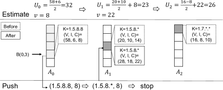
Figure 6: Example of the Detect operation in MVPipe.

III-C 2D HHH Detection

We extend MVPipe to 2D HHH detection, in which the generalization relation now forms a lattice structure (Figure 1(b)). Similar to 1D HHH detection, we maintain an array of buckets for each node of the lattice to track the candidate HHHs. We briefly describe the Update and Detect operations in 2D HHH detection; their pseudo-code is in the supplementary file.

Update operation.

In 2D HHH detection, we need to address the generalization order and the stop condition in the Update operation. Unlike 1D HHH detection, which only has one generalization direction, a key in 2D HHH detection has two generalization directions: the source direction (i.e., from left to right) and the destination direction (from bottom to up). For example, the address pair (1.2.3.4, 5.6.7.8) can be generalized to either (1.2.3.*, 5.6.7.8) or (1.2.3.4, 5.6.7.*) by a single byte. To represent the lattice structure in MVPipe, we index the arrays of MVPipe first along the destination direction (from bottom to up), followed by along the source direction (from left to right). For example, array $A_{0}$ corresponds to node (0,0), while array $A_{22}$ corresponds to node (4,2) in Figure 1(b) (recall that the number of arrays is the number of nodes in the lattice).

We enforce that the generalization of a key along the source direction only applies to the bottom nodes in the lattice (i.e., nodes (0,0), (0,1), …, (0,4) in Figure 1(b)). Specifically, we update each incoming packet in MVPipe starting from level 0 (i.e., node (0,0)). If a key is not admitted by a candidate HHH, we push the key in two generalization directions: (i) along the destination direction from the bottom node and (ii) the next bottom node. We stop the generalization until a key is admitted by the candidate HHH in a bottom node.

We use Figure 7 to show the idea of the Update operation. For the key (1.2.3.4, 5.6.7.8), we first insert it to array $A_{0}$ in node (0,0). If it is not a candidate HHH, we push the key along the destination direction until it is admitted by some ancestor (e.g., node $o$). We also push the key to the next bottom node (1,0). If, say, the generalized key (1.2.3.*, 5.6.7.8) is still not a candidate HHH, we push it along the destination direction until it is admitted by some ancestor (e.g., node $x$). Similar operations apply to node (2,0) and its destination direction. We terminate until the key is admitted by a bottom node (e.g., node $p$).

Detect operation.

Since we now push the count of a key along both the source direction along the bottom nodes and the destination direction from the bottom nodes, the count of a key can contribute to multiple ancestors, leading to the double counting problem [11, 24]. For example, the key (1.2.3.4, 5.6.7.8) is pushed along the arrows in Figure 7 according to the Update operation. Suppose that its count is counted by both of its ancestors $x$ and $y$ that are both reported to be HHHs. Now, we calculate the conditioned count of $z$, which is the common ancestor of both $x$ and $y$. By the definition of the conditioned count, we need to subtract the counts of both $x$ and $y$ from $z$, but doing so will deduct the count of (1.2.3.4, 5.6.7.8) twice from $z$.

The Detect operation addresses the double counting problem based on the inclusion-exclusion principle [11, 24], whose idea is that after subtracting all descendants that are HHHs, we add back the count that is discounted twice. At the end of an epoch, the Detect operation checks the candidate HHH in each bucket. If the estimated conditioned count of a candidate HHH exceeds the threshold, we add it to the output set; otherwise, we push the candidate HHH to higher-level nodes, either in the source direction along the bottom nodes or in the destination direction from the bottom nodes.

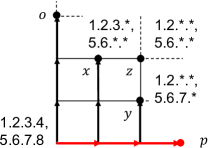
Figure 7: Illustration for the major operations in 2D HHH detection. The generalization is applied either in the source direction along the bottom nodes or in the destination direction from the bottom nodes.

III-D Discussion

MJRTY has also been adopted in HH detection (i.e., no hierarchy awareness) [18, 35]. In particular, MV-Sketch [35] maintains multiple rows of buckets, in which each bucket tracks a candidate HH using MJRTY. It hashes each packet into a bucket in each of the rows, and updates the counters in each bucket. It uses multiple rows of buckets to resolve the hash collisions of HHs into the same bucket. In contrast to MVPipe, MV-Sketch implements a single stage of MJRTY and is not hierarchy-aware, while MVPipe forms multiple pipelined stages of MJRTY for HHH detection.

MVPipe is much beyond a simple extension of MV-Sketch in HHH detection. A naïve way to extend MV-Sketch for HHH detection is to maintain an instance of MV-Sketch for every node of the IP address hierarchy. For each packet, we compute all its generalizations and insert each of them independently into the corresponding instances, so that the HHHs can later be recovered as the HHs of each aggregation level. However, such a naïve approach incurs substantial update overhead, as it updates all MV-Sketch instances for each incoming packet. In contrast, MVPipe forms multiple pipelined stages of MJRTY that correspond to different nodes in the IP address hierarchy, and maintains one array for each node. With the skewness of IP traffic, MVPipe only needs to update a small number of arrays per packet (and one array for most of the time) and hence achieves lightweight updates. Also, to resolve hash collisions, MVPipe checks additional arrays in higher levels when estimating the value of a candidate HHH (see the Estimate function in Figure 4) and hence maintains high accuracy.

Currently, we focus on 1D and 2D HHH detection. MVPipe can be extended for higher dimensions, yet both its space and time complexities become the multiplication of the depths of all dimensions. Nevertheless, practical applications do not need to consider general HHH detection in all dimensions [39].

In addition, the examples presented in this paper are based on IPv4 traffic, yet MVPipe can also be directly applied to IPv6 traffic without modification. We present our evaluation results for IPv6 traffic in the supplementary file.

IV Implementation

We have implemented MVPipe in both software and hardware. In particular, our hardware implementation of MVPipe is written in P4 [28], and addresses the limitations of the existing hardware-based HHH detection schemes (§I) in the following ways: no reliance on a controller for counter updates, using SRAM rather than TCAM (which is more expensive and scarce) for HHH counting, and avoids sampling of packets or aggregation levels for fast convergence.

IV-A Software Implementation

We have built a software version of MVPipe in C++ with around 800 LoC (including both 1D and 2D HHH detection). MVPipe uses MurmurHash [1] as the hash function. It can be integrated into the data plane of a software switch [29] for real-time HHH detection. Specifically, the software switch inserts the IP packet header of each incoming packet to an in-memory buffer, from which MVPipe fetches and processes the packet headers. We now implement MVPipe in a single thread running on a single CPU core.

IV-B P4 Implementation

We implement MVPipe in P4 [28] with around 900 LoC and compile it into a Tofino switch [36]. Our P4 implementation is based on the Protocol Independent Switch Architecture (PISA) [6, 5]. A PISA switch first extracts the header fields of each incoming packet via a programmable parser. It then passes the packet to an ingress pipeline of stages, each of which contains a series of match-action tables. Each stage matches the extracted header fields of the packet with the entries in the match-action tables, and applies the matched actions to modify the extracted header fields and/or update the persistent state at the stage. Afterwards, the switch passes the packet to a similar egress pipeline and emits the packet.

Programmable switches offer rich computational capability in addition to packet forwarding, yet they pose stringent hardware resource constraints [4]. For example, a programmable switch typically has limited SRAM (e.g., few megabytes) and a small number of stateful arithmetic-logic units (ALUs) per stage. Such constraints pose two challenges to our MVPipe implementation. First, each stage in the ingress/egress pipeline can only access a memory block once per packet, with only a single read-modify-write operation. Second, each stage only supports an if-else chain with at most two branches.

In the following, we describe how we address the above constraints and adapt MVPipe into a programmable switch. Here, we only focus on the 1D-byte HHH detection due to the limited number of stages available in a switch, while the detection for other granularities is posed as future work. For each level of the 1D-byte hierarchy, we create four register arrays, denoted by $K$, $V$, $I$, and $C$, which correspond to the four bucket fields in MVPipe (Figure 3).

Using pairs atoms to update dependent fields.

One implementation challenge is that the Push function (Figure 4) makes inter-dependent accesses to $K$ and $I$: the write to $I$ depends on the value of $K$ (Lines 6-7), yet the write to $K$ is conditioned on the value of $I$ (Lines 12-14). It is infeasible to update both $K$ and $I$ with a single read-modify-write.

We resolve the inter-dependency of updating both $K$ and $I$ using the pairs atoms [33], which are natively supported atomic operations in PISA. A pairs atom reads two 32-bit elements from a register array, performs conditional branching and primitive arithmetic on both elements, and writes back the results. At the same time, it can output either the original value of an element or the computation results to a specified metadata field. In our case, we pack $K$ and $I$ to the upper 32 bits and lower 32 bits in a 64-bit register array, respectively. We then update them using a pairs atom.

Reducing the updates to the indicator counter.

Referring to the Push function in Figure 4, we split the updates to the bucket fields into three branches: Lines 6-9, Lines 10-11, and Lines 12-14. Only the indicator counter (i.e., the register array $I$) will be updated in each of the three branches. This needs a three-branch if-else chain to update $I$, which is infeasible as only a two-branch if-else chain is supported in each stage.

To fit the update of $I$ into a two-branch if-else chain, we discard the update of $I$ in the third branch (i.e., Line 13 in Figure 4); in other words, the indicator counter will not be updated if a key is not a candidate HHH in $K$ but has a count larger than the current indicator counter $I$. The rationale here is that the condition rarely happens in skewed workloads, in which an HHH is quickly tracked in $K$ and is unlikely (albeit possible) substituted by a different key. Thus, we (slightly) sacrifice the accuracy to reduce the update of $I$ to only two (instead of three) branches. Now all bucket fields can be updated with a two-branch if-else chain in a single stage.

1:function Push($l$)

2:    $(x,v_{x})\leftarrow$ (Meta.key_l, Meta.val_l)

3:    // Stage 1: update $V_{l,h(x)}$ and $(K_{l,h(x)},I_{l,h(x)})$

4:    $V_{l,h(x)}\leftarrow V_{l,h(x)}+v_{x}$

5:    if $K_{l,h(x)}=x$ then $\triangleright$ Case 1

6:         $I_{l,h(x)}\leftarrow I_{l,h(x)}+v_{x}$

7:    else$\triangleright$ Case 2

8:         $I_{l,h(x)}\leftarrow I_{l,h(x)}-v_{x}$     

9:    if $K_{l,h(x)}\neq x$ and $I_{l,h(x)}<v_{x}$ then $\triangleright$ Case 3

10:         $K_{l,h(x)}\leftarrow x$     

11:    if $K_{l,h(x)}=x$ or $I_{l,h(x)}<v_{x}$ then $\triangleright$ Case 1 or 3

12:         Meta.key_(l+1) $\leftarrow K_{l,h(x)}$     

13:    // Stage 2: set metadata fields based on the last Stage

14:    if Meta.key${}_{(l+1)}=0$ then $\triangleright$ Case 2

15:         Meta.key_(l+1) $\leftarrow$ generalize $x$ at level $l+1$

16:         Meta.val_(l+1) $\leftarrow v_{x}$

17:    else

18:         Meta.flag${}_{l}\leftarrow$ Meta.key_(l+1) xor $x$     

19:    // Stage 3: update $C_{l,h(x)}$ based on metadata set in Stage 2

20:    if Meta.flag${}_{l}=0$ then $\triangleright$ Case 1

21:         $C_{l,h(x)}\leftarrow C_{l,h(x)}+v_{x}$

22:    else$\triangleright$ Case 3

23:         Meta.val${}_{(l+1)}\leftarrow C_{l,h(x)}$

24:         $C_{l,h(x)}\leftarrow v_{x}$

25:         Meta.key${}_{(l+1)}\leftarrow$ generalize Meta.key_(l+1) at level $l+1$     

26:procedure Update

27:    Push($0$)

28:    if Meta.val${}_{1}\neq 0$ then

29:         Push($1$)     

30:    if Meta.val${}_{2}\neq 0$ then

31:         Push($2$)     

32:    if Meta.val${}_{3}\neq 0$ then

33:         Push($3$)     

34:    if Meta.val${}_{4}\neq 0$ then

35:         $V_{4}\leftarrow V_{4}+$ Meta.val₄     

Figure 8: Pseudo-code of the update operation for 1D-byte HHH detection in P4.

Putting it all together.

Figure 8 shows the pseudo-code of our P4 implementation. For each level $l$, where $0\leq l\leq 4$, we denote the corresponding register arrays by $K_{l}$, $V_{l}$, $I_{l}$, and $C_{l}$, where each element of $K_{l}$ is initialized as $-1$ and each element of other arrays is initialized as zero. We define three metadata fields for level $l$, namely Meta.key_l, Meta.value_l, and Meta.flag_l. The metadata fields Meta.key_l and Meta.value_l store the key and its value, respectively, that are pushed to level $l$, while Meta.flag_l stores the intermediate result at level $l$. All metadata fields are initialized as zeros prior to the processing of each packet.

The Push function pushes the key Meta.key_l and the value Meta.val_l to level $l$ in three stages:

• Stage 1: update $(K_{l},I_{l})$ with a pairs atom;

• Stage 2: set the metadata value using the results in Stage 1; and

• Stage 3: update $C_{l}$ and prepare the key and value that should be pushed to the next level based on the metadata value from Stage 2.

We denote the three branches in the Push function (i.e., Lines 6-9, Lines 10-11, and Lines 12-14 in Figure 4) by Case 1, Case 2 and Case 3, respectively. In Stage 1, we issue a pairs atom to perform conditional branching on $K_{l,h_{l}(x)}$ and $I_{l,h_{l}(x)}$ and update their values accordingly. Each time when Case 1 or Case 3 happens, we output the original value of $K_{l,h_{l}(x)}$ to Meta.key_l+1 (Lines 11-12). Note that all conditional branches in a pairs atom are executed simultaneously. In Stage 2, if Meta.key_(l+1) equals zero (i.e., neither Case 1 nor Case 3 happens), we set Meta.key_(l+1) as the generalization of $x$ at level $l+1$ and Meta.val_(l+1) as $v_{x}$ (Line 14-16). Otherwise, we set Meta.flag_l as 0 if $x$ equals Meta.key_(l+1) (Case 1), or 1 if they are different (Case 2) (Line 18). In Stage 3, we update $C_{l,h(x)}$ based on the value of Meta.flag_l (Lines 20-25).

To realize the Update procedure of MVPipe in P4, we call Push($0$) to update each packet from level $0$ (Line 27). If Meta.val₁ has a non-zero value in Push($0$) (i.e., either Case 2 or Case 3 happens), we continue to call Push($1$) to update level $1$ (Lines 28-29). We have a similar process for level 2 and level 3 (Lines 30-33). For level 4, we maintain only one register to count the value of Meta.val₄, as there is only one fully generalized key (i.e., any address) (Lines 34-35).

V Theoretical Analysis

We present theoretical analysis on MVPipe for both 1D and 2D HHH detection. Our analysis configures MVPipe with $\tfrac{2}{\epsilon}$ buckets per array on average and the number of ancestors being checked in estimation $t=\log\tfrac{1}{\delta}$ ($t$ is defined in §III-B), where $\epsilon$ ($0<\epsilon\leq\phi<1$) is the approximation parameter, $\delta$ ($0<\delta<1$) is the error probability, and the logarithm base is 2. Each key is represented in $\log n$ bits, where $n$ is the maximum value of a key. We use the same $n$ for both 1D and 2D cases.

Our analysis assumes $H\geq t=\log\tfrac{1}{\delta}$ (where $H$ is the number of nodes in the hierarchy, or the number of arrays in MVPipe, as defined in §III-A). That is, MVPipe has sufficient memory to cover all nodes in the hierarchy for accurate HHH detection.

V-A Main Results

Our goal is to show that MVPipe maintains the following two properties.

• Accuracy: $\Pr[\hat{S}(x)-S(x)\leq k\epsilon\mathcal{S}]>1-\tfrac{1}{4k}$, for some constant $k\geq 1$. This property states that the estimated count of a key in MVPipe is close to its true count with a high probability.

• Coverage: For each key $x\notin\mathcal{H}$, $S_{\mathcal{H}}(x)<\phi\mathcal{S}$. This property states that any key not in the output set of HHHs $\mathcal{H}$ must have a conditioned count with respect to $\mathcal{H}$ less than $\phi\mathcal{S}$.

We first bound the count of a key in a bucket to which the key is hashed. Let $\Delta(x)$ be the true count of $x$ tracked in its hashed bucket $B(i,j)$. Lemma 1 gives both the upper and lower bounds of $\Delta(x)$. Lemma 2 further shows that $U(x)$ given by the Estimate function is an upper bound of $\Delta(x)$.

Lemma 1.

Consider the bucket $B(i,j)$ to which key $x$ is hashed. If $K_{i,j}$ equals $x$, then $C_{i,j}\leq\Delta(x)\leq\tfrac{V_{i,j}+I_{i,j}}{2}$; otherwise, $0\leq\Delta(x)\leq\tfrac{V_{i,j}-I_{i,j}}{2}$.

Proof.

We can bound $\Delta(x)$ with the values of $K_{i,j}$ and $I_{i,j}$ based on the prior analysis [35, Lemma 2] on MJRTY [7]. If $x$ equals $K_{i,j}$, $I_{i,j}\leq\Delta(x)\leq\tfrac{V_{i,j}+I_{i,j}}{2}$; otherwise, $0\leq\Delta(x)\leq\tfrac{V_{i,j}-I_{i,j}}{2}$. In MVPipe, if $x$ equals $K_{i,j}$, we use $C_{i,j}$ to track the cumulative count of $x$ since it is stored in $K_{i,j}$, which implies $\Delta(x)\geq C_{i,j}\geq I_{i,j}$. ∎

Lemma 2.

The returned estimate $U(x)$ of key $x$ by the Estimate function is an upper bound of $\Delta(x)$.

Proof.

We focus on 1D HHH detection, while the proof for 2D HHH detection is identical. Denote the $t$ closest ancestors of $x$ by $y_{i}$, where $1\leq i\leq t$. Let $U_{x}$ and $U_{i}$ be the temporary estimates calculated for $x$ and $y_{i}$ in the Estimate function, respectively. By Lemma 1 and the Estimate function, we have $U_{x}\geq\Delta(x)$ and $U_{i}\geq\Delta(y_{i})+v\geq\Delta(x)$, where $v$ is the sum of cumulative counts of $y_{i}$’s descendants. Thus, $U(x)=\min_{1\leq i\leq t}{\{U_{x},U_{i}\}}\geq\Delta(x)$. ∎

We first consider 1D HHH detection. Theorem 1 states the space and time complexities of MVPipe. Theorem 2 shows that MVPipe satisfies both accuracy and coverage properties. Theorem 3 further presents the bounds of MVPipe for 1D HHH detection under certain conditions.

Theorem 1.

In 1D HHH detection, MVPipe finds HHHs in $O(\tfrac{H}{\epsilon}\log{n})$ space. The update time is $O(H)$. The detection time is $O(\tfrac{H(d-1)}{\epsilon}\log{\tfrac{1}{\delta}})$. Note that the space and time complexities of MVPipe are implicitly related to the error probability $\delta$, as we assume $H\geq\log{\tfrac{1}{\delta}}$.

Proof.

We maintain an array of buckets for each of the $H$ nodes in the hierarchy. Each bucket stores a $\log n$-bit candidate HHH and three counters. Thus, the space usage is $O(\tfrac{H}{\epsilon}\log{n})$. Each per-packet update accesses at most $H$ buckets, and hence takes $O(H)$ time in the worst case. We traverse all $Hw$ buckets to return the set of HHHs. For each candidate HHH $x$ in a bucket, we obtain $\hat{S}_{\mathcal{H}}(x)$ by checking the $t$ closest ancestors of $x$. If $\hat{S}_{\mathcal{H}}(x)$ is below the threshold, we push $x$ to at most $d-1$ higher-level arrays. Thus, it takes $O(\tfrac{H(d-1)}{\epsilon}\log{\tfrac{1}{\delta}})$ time to return all HHHs. ∎

Theorem 2.

The main operations of MVPipe in 1D HHH detection (Figure 4 in §III-B) satisfy the accuracy and coverage properties.

Proof.

We first prove the accuracy property. Let $B(i,j)$ be the bucket to which $x$ is hashed. Consider the sum of all keys in $B(i,j)$ except $x$. Its expectation is $\mathbf{E}[V_{i,j}-\Delta(x)]=\mathbf{E}[\sum_{y\neq x,h_{i}(y)=h_{i}(x)}\Delta(y)]\leq\tfrac{\mathcal{S}-\Delta(x)}{w_{i}}\leq\tfrac{\epsilon\mathcal{S}}{2}$. By Markov’s inequality,

$$\Pr[V_{i,j}-\Delta(x)\geq k\epsilon\mathcal{S}]\leq\tfrac{1}{2k}.$$ (1)

We study the difference between $S(x)$ and $\hat{S}(x)$. When we start checking $B(i,j)$ in the Detect operation, the counts of the descendants of $x$ that are not in $\mathcal{H}$ are all pushed to $B(i,j)$. At this time, $S(x)$ consists of two parts in MVPipe: $\Delta(x)$; and the sum of the cumulative counts of $x$’s descendants in $\mathcal{H}$. That is, $S(x)=\Delta(x)+\sum_{x^{\prime}\in\mathcal{H}\wedge x^{\prime}\prec x}C_{i^{\prime},h_{i^{\prime}}(x^{\prime})}$, where $i^{\prime}$ is the level of $x^{\prime}$. By the Detect operation, $\hat{S}(x)=U(x)+\sum_{x^{\prime}\prec x\wedge x\in\mathcal{H}}C_{i^{\prime},h_{i^{\prime}}(x^{\prime})}$. We then have $\hat{S}(x)-S(x)=U(x)-\Delta(x)$. By Lemma 1 and the Estimate function, if $K_{i,j}$ equals $x$, $U(x)-\Delta(x)\leq\tfrac{V_{i,j}+I_{i,j}}{2}-\Delta(x)\leq\tfrac{V_{i,j}-\Delta(x)}{2}$; otherwise, if $K_{i,j}\neq x$, $U(x)-\Delta(x)\leq\tfrac{V_{i,j}-I_{i,j}}{2}-\Delta(x)\leq\tfrac{V_{i,j}-\Delta(x)}{2}$. Combining both cases, we have $\Pr[U(x)-\Delta(x)\geq k\epsilon\mathcal{S}]\leq\Pr[\tfrac{V_{i,j}-\Delta(x)}{2}\geq k\epsilon\mathcal{S}]\leq\tfrac{1}{4k}$ by Equation 1. Thus, $\Pr[\hat{S}(x)-S(x)\leq k\epsilon\mathcal{S}]=\Pr[U(x)-\Delta(x)\leq k\epsilon\mathcal{S}]\geq 1-\tfrac{1}{4k}$.

We prove the coverage property by contradiction. Suppose that $S_{\mathcal{H}}(x)\geq\phi\mathcal{S}$. As the counts of the descendants of $x$ that are not in $\mathcal{H}$ must be pushed to $B(i,j)$, we have ${S}_{\mathcal{H}}(x)\leq\Delta(x)$. Then, $\phi\mathcal{S}\leq{S}_{\mathcal{H}}(x)\leq\Delta(x)\leq U(x)=\hat{S}_{\mathcal{H}}(x)$. We do not report $x$ as an HHH only if $x$ is not stored in $K_{i,j}$. In this case, the count of $x$ in $B(i,j)$ is further pushed to its ancestors until $x$ is admitted by an HHH. Thus, we must add at least one of the ancestors of $x$ to $\mathcal{H}$. By the definition of the conditioned count, $S_{\mathcal{H}}(x)=0$, which is a contradiction. ∎

Theorem 3.

In 1D HHH detection, if key $x$ and each of its $t=\log\tfrac{1}{\delta}$ closest ancestors have counts at most $(\phi-\tfrac{\epsilon}{2})\mathcal{S}$, MVPipe falsely reports $x$ as an HHH with a probability at most $\delta$; if $x$ is at level $l$ with $S_{\mathcal{H}_{l-1}}(x)\geq\phi\mathcal{S}$, MVPipe misses $x$ and reports its ancestor at a level higher than $l+t$ as an HHH with a probability at most $\delta$.

Proof.

We first show that MVPipe reports a small key $x$ that is at level $l$ with a small probability. Suppose that $x$ is hashed to bucket $B(l,j)$. A necessary condition of reporting $x$ as an HHH is that $\hat{S}_{\mathcal{H}_{l-1}}(x)=U(x)\geq\phi\mathcal{S}$. We get $U(x)=\min\{U_{k}\}$, where $0\leq k\leq t$ and $U_{0},U_{1},\dots,U_{t}$ are the estimate of $x$ and its $t$ ancestors $y_{1},\dots,y_{t}$, respectively, in the Estimate function. We have $U_{k}\geq\phi\mathcal{S}$ for each $0\leq k\leq t$. Consider $U_{0}$ first. We have $U_{0}-S(x)\geq\phi\mathcal{S}-(\phi-\tfrac{\epsilon}{2})\mathcal{S}=\tfrac{\epsilon\mathcal{S}}{2}$. Then, $\Pr[U_{0}-S(x)\geq\tfrac{\epsilon\mathcal{S}}{2}]\leq\Pr[U_{0}-\Delta(x)\geq\tfrac{\epsilon\mathcal{S}}{2}]\leq\Pr[\tfrac{V_{i,j}-\Delta(x)}{2}\geq\tfrac{\epsilon\mathcal{S}}{2}]\leq\tfrac{1}{2}$ by Equation 1 and the proof in Theorem 2. Similarly, we can get $\Pr[U_{k}-S(y_{k})\geq\tfrac{\epsilon\mathcal{S}}{2}]\leq\tfrac{1}{2}$. Thus, $\Pr[U(x)\geq\phi\mathcal{S}]=\prod_{k=0}^{t}\Pr[U_{k}-S(y_{k})\geq\tfrac{\epsilon\mathcal{S}}{2}]\leq\tfrac{1}{2^{t+1}}\leq\delta$.

We show that MVPipe misses an HHH $x$ at level $l$ but reports its ancestor at much higher levels with a small probability. Given $S_{\mathcal{H}_{l-1}}(x)\geq\phi\mathcal{S}$, we have $\hat{S}_{\mathcal{H}_{l-1}}(x)=U(x)\geq\Delta(x)\geq S_{\mathcal{H}_{l-1}}(x)\geq\phi\mathcal{S}$ by the Detect operation and Lemma 2. We do not report $x$ as an HHH when checking its hashed bucket $B(l,j)$ if $x$ is not stored in $K_{l,j}$. By MJRTY, the count of $x$ in $B(l,j)$ does not account for more than half of the total count in that bucket. We have $\Pr[\Delta(x)\leq\tfrac{V_{l,j}}{2}]=\Pr[V_{l,j}-\Delta(x)\geq\Delta(x)]\leq\Pr[V_{l,j}-\Delta(x)\geq S_{\mathcal{H}}(x)]\leq\Pr[V_{l,j}-\Delta(x)\geq\phi\mathcal{S}]\leq\Pr[V_{l,j}-\Delta(x)\geq\epsilon\mathcal{S}]\leq\tfrac{1}{2}$ by Equation 1. Similarly, the probability that we miss the next ancestor of $x$ is also smaller than $\tfrac{1}{2}$. Thus, the probability that we miss all $t-1$ closest ancestors of $x$ is smaller than $\tfrac{1}{2^{t}}=\delta$. ∎

We also consider 2D HHH detection. Theorem 4 states the space and time complexities. Theorem 5 shows that MVPipe satisfies both the accuracy and coverage properties. In the interest of space, we present the major operations of 2D HHH detection and the proofs of the theorems in the supplementary file.

Theorem 4.

In 2D HHH detection, MVPipe finds HHHs in $O(\tfrac{H}{\epsilon}\log{n})$ space. The update time is $O(d)$ in the worst case. The detection time is $O(\tfrac{(d-1)H}{\epsilon}\log{\tfrac{1}{\delta}})$.

Theorem 5.

The main operations of MVPipe in 2D HHH detection satisfy the accuracy and coverage properties.

V-B Comparisons with Existing Schemes

Update time. Compared to previous studies, except for RHHH [3] with $O(1)$ update time, MVPipe achieves the same or even a lower update time complexity even in the worst case. For example, the schemes in [24] process each packet at each of the $H$ nodes in the hierarchy, and the update time complexity is $O(H\log\tfrac{1}{\epsilon})$ (for heap-based implementation) and $O(H)$ (using unitary updates). The schemes in [11] have an amortized update time complexity $O(H\log{(\epsilon\mathcal{S})})$.

Note that our update time analysis for MVPipe in Theorem 1 focuses on the worst case (i.e., each packet update takes $O(H)$ time), yet our evaluation (i.e. Experiments 4 and 5 in §VI) shows that MVPipe can terminate the Update operation for most packets at low levels under the skewness of IP traffic. The amortized update time of MVPipe in our evaluation for real-world traces is much smaller than $O(H)$.

Accuracy.

Prior studies pose strong accuracy guarantees for the estimated count $\hat{S}(x)$ of key $x$. For example, the HHH detection schemes in [11, 24] guarantee that the error between $\hat{S}(x)$ and $S(x)$ is at most $\epsilon\mathcal{S}$, while randomized HHH (RHHH) [3] keeps the error within $\epsilon\mathcal{S}$ with a probability of at least $1-\delta$. In contrast, MVPipe relaxes the accuracy guarantee for high update performance, in which $\hat{S}(x)$ is close to $S(x)$ and deviates much from $S(x)$ with a small probability.

We can improve the accuracy of MVPipe by maintaining multiple rows of buckets for each node of the hierarchy, at the expense of degrading the processing speed and increasing the update complexity. The reasons are two-fold. First, the process of each key in an array of MVPipe requires multiple memory accesses, as MVPipe needs to insert each processed key into multiple arrays to reduce the errors caused by hash collisions. Second, there could be multiple keys being kicked out from an array after a key is updated, and if it happens, we need to further check whether each of the kicked-out keys remains in the other rows of the array except for the row where the key is kicked out. When we push the kicked-out keys that are no longer in the array to the subsequent higher-level arrays, each of these keys may also kick out multiple keys. Thus, maintaining multiple rows of buckets for each node of the hierarchy incurs high update overhead. Nevertheless, even though the one-row-array design of MVPipe relaxes the accuracy guarantee, our evaluation (i.e., Experiments 1 and 2 in §VI) shows that MVPipe achieves high accuracy.

VI Evaluation

We compare MVPipe with six state-of-the-art HHH detection schemes, including: trie-based HHH detection (TRIE) [39], full ancestry (FULL) [11], partial ancestry (PARTIAL) [11], heap-based Space Saving (HSS) [24], unitary-update-based Space Saving (USS) [24], and randomized HHH (RHHH) [3]; the first five schemes are streaming-based, while RHHH is sampling-based (§I). We show that MVPipe achieves (i) high detection accuracy, (ii) high update throughput, (iii) small convergence time, and (iv) limited resource usage in a Tofino switch [36].

VI-A Methodology

Traces. We use the real-world traces from CAIDA [8], captured on an OC-192 backbone link in January 2019. Note that CAIDA traces are also used for evaluating HHH detection in both networking [3] and database [11, 24] communities. By default, we use the first five minutes of the traces for evaluation and divide them into five one-minute epochs, each of which has 36.7 M packets and 1.1 M unique IPv4 addresses on average; in Experiment 6, we vary the number of epochs and the epoch length. We perform HHH detection in each epoch and obtain the average results over all epochs.

We also consider IPv6 traffic from both the CAIDA traces and the IPv6 traces from MAWI’s WIDE project[10]. We find that MVPipe shows similar trends on both IPv4 and IPv6 traffic compared with state-of-the-arts. For brevity, we focus on IPv4 traffic in the CAIDA traces in this section, and report the findings for IPv6 traffic in the supplementary file.

Parameter settings.

We configure the number of buckets (i.e., $w_{i}$) in each array $A_{i}$ of MVPipe for a given available memory size, where $0\leq i<H$. We first calculate the average number of buckets, denoted by $w_{avg}$, for each array of MVPipe based on the bucket size (e.g, a bucket consumes 16 bytes, with four bytes for each field, for 1D-byte HHH detection) and the number of nodes $H$ in the hierarchy (e.g., five nodes for 1D-byte HHH detection). We set $w_{i}$ for each array $A_{i}$, starting from the top level $H-1$ of the hierarchy. If a level has a key space size smaller than $w_{avg}$ (e.g., the highest level $H-1$ has only the wildcard element), we set $w_{i}$ as the key space size and update $w_{avg}$ by averaging the residual available memory size among the remaining arrays; otherwise, we set $w_{i}=w_{avg}$.

We configure the memory sizes for HSS, USS, and RHHH based on the fractional threshold $\phi$ to ensure that there is enough memory to store the maximum possible number of HHHs; a large $\phi$ implies a small number of true HHHs in an epoch, which also implies less memory usage to store all HHHs. We also configure the maximum memory sizes for FULL and PARTIAL based on $\phi$. Note that the memory sizes for FULL and PARTIAL vary in an epoch, as they dynamically expand and shrink their counter arrays during packet processing to keep only the large keys in the arrays.

We consider 1D-byte, 1D-bit, 2D-byte, and 2D-bit HHH detection. We only present the results for packet counting (i.e., $v_{f}=1$) in the interest of space, while MVPipe shows similar results for byte counting. For TRIE, we only evaluate it for 1D cases, due to its high space complexity and low accuracy for 2D cases. We implement hash functions using MurmurHash [1] in all schemes.

VI-B Results

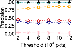
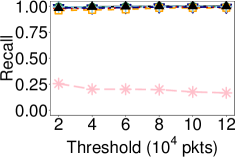
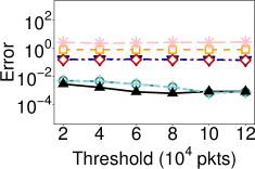
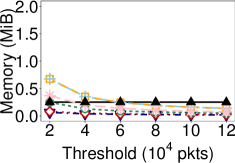
(a) Precision for 1D-byte	(b) Recall for 1D-byte	(c) Error for 1D-byte	(d) Memory for 1D-byte
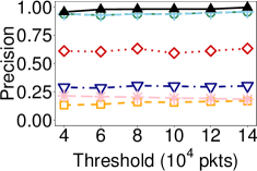
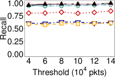
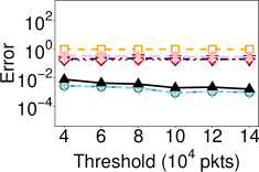
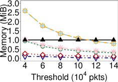
(e) Precision for 1D-bit	(f) Recall for 1D-bit	(g) Error for 1D-bit	(h) Memory for 1D-bit
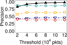
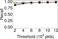
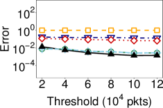
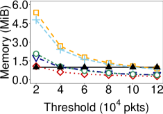
(i) Precision for 2D-byte	(j) Recall for 2D-byte	(k) Error for 2D-byte	(l) Memory for 2D-byte
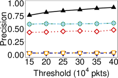
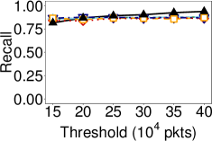
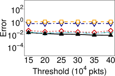
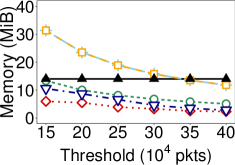
(m) Precision for 2D-bit	(n) Recall for 2D-bit	(o) Error for 2D-bit	(p) Memory for 2D-bit

Figure 9: (Experiment 1) Accuracy comparisons.

(Experiment 1) Accuracy comparisons. We compare different HHH detection schemes on accuracy versus different values of the absolute threshold $\phi\mathcal{S}$. We fix the memory space of MVPipe as 256 KiB, 1 MiB, 1 MiB, and 16 MiB for 1D-byte, 1D-bit, 2D-byte, and 2D-bit HHH detection, respectively. We consider different absolute thresholds, such that the number of true HHHs per epoch varies between 200 and 1,000.

We consider three accuracy metrics: (i) precision, the ratio of true HHHs reported over all reported HHHs (the denominator includes all true and false HHHs); (ii) recall, the ratio of true HHHs reported over all true HHHs (the denominator includes all reported and non-reported true HHHs); and (iii) relative error, defined as $\tfrac{1}{|\mathcal{H}|}\sum_{x\in\mathcal{H}}\tfrac{|\hat{S}(x)-S(x)|}{S(x)}$, where $\mathcal{H}$ is the set of true HHHs reported. Note that an HHH is identified by both its prefix and subnet mask. For example, it is treated as an error if an HHH 1.2.3.4/32 is reported as 1.2.3.4/31 in 1D-bit HHH detection.

We also measure the memory usage of each scheme based on the number of counters allocated in its data structure. As both FULL and PARTIAL dynamically allocate memory space in each epoch, we report their peak memory usage.

Figure 9 shows the results. MVPipe achieves higher accuracy in most cases compared to others in all cases. RHHH achieves a precision below 0.85 and 0.25 for byte-level and bit-level HHH detection, respectively, with a relative error of around 100%. The reason is that RHHH has slow convergence and needs to process sufficient packets in order to converge to high accuracy (see Experiment 6 for further analysis). Both HSS and USS have comparable accuracy to MVPipe in 1D-byte and 1D-bit HHH detection, yet their precisions are significantly lower than MVPipe in 2D-byte and 2D-bit HHH detection (e.g., their precisions are around 0.6 in 2D-bit precision), mainly because they estimate the conditioned count of a key in a more conservative way. TRIE, FULL, and PARTIAL have low accuracy in all settings. We observe that the accuracy of MVPipe increases with the threshold (i.e., fewer HHHs), while those of other schemes remain almost the same for all thresholds. The reason is that MVPipe adopts static memory allocation and its memory size is fixed for all thresholds, while the memory sizes of other schemes decrease as the threshold increases (§VI-A).

For memory usage, MVPipe maintains a medium size of memory usage among all schemes. RHHH and USS have the highest memory usage in most cases, as they implement multiple Space Saving instances [23], each of which comprises a hash table and multiple doubly linked lists. FULL and PARTIAL have the smallest memory usage, as they dynamically kick out small keys and keep only large keys in their counter arrays; however, such dynamic memory allocation incurs high update overhead (Experiment 3).

(Experiment 2) Robustness of MVPipe under various memory sizes.

We evaluate MVPipe versus the absolute threshold $\phi\mathcal{S}$ by varying the memory size allocated for MVPipe. We configure the memory size in the range from 256 KiB to 2 MiB for 1D-byte, 1D-bit, and 2D-byte HHH detection, while increasing the memory size to the range from 8 MiB to 14 MiB for 2D-bit HHH detection for tracking many more nodes in the 2D-bit hierarchy.

Figure 10 shows the results. As expected, MVPipe achieves higher accuracy with larger memory sizes. Also, the accuracy of MVPipe is fairly robust in different cases. For example, with a memory size of 1 MiB, both the precision and recall of MVPipe are above 0.9 for most of the absolute threshold settings in 1D-bit, 1D-byte, and 2D-byte HHH detection.

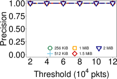
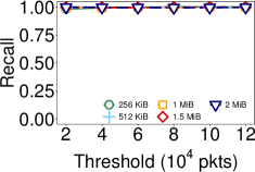
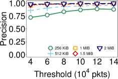
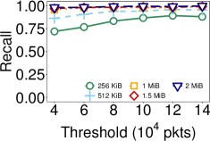
(a) Precision for 1D-byte	(b) Recall for 1D-byte	(c) Precision for 1D-bit	(d) Recall for 1D-bit
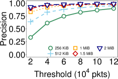
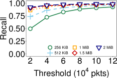
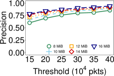
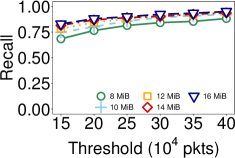
(e) Precision for 2D-byte	(f) Recall for 2D-byte	(f) Precision for 2D-bit	(h) Recall for 2D-bit

Figure 10: (Experiment 2) Robustness of MVPipe under various memory sizes.

(Experiment 3) Update throughput.

We benchmark the update throughput of all HHH detection schemes on a server equipped with an Intel Xeon E5-1630 3.70 GHz CPU and 16 GiB RAM. The server runs Ubuntu 14.04.5. To exclude disk I/O overhead and stress-test each scheme, we first load the whole trace into memory before running the experiment, and then process the trace as fast as possible. Here, we focus on 1D-byte and 1D-bit HHH detection, while similar performance trends are observed for 2D-byte and 2D-bit HHH detection. We keep the same memory size setting for MVPipe as in Experiment 1 and fix the absolute threshold as 100,000 packets.

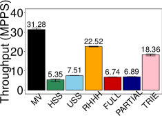
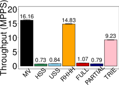
(a) 1D-byte	(b) 1D-bit

Figure 11: (Experiment 3) Update throughput.

Figures 11(a) and 11(b) show the update throughput of all schemes in million packets per second (MPPS) for 1D-byte and 1D-bit HHH detection, respectively; each error bar shows the maximum and minimum throughput across different epochs for each scheme. MVPipe achieves the highest throughput with up to $5.84\times$ and $22.13\times$ throughput gain for byte-level and bit-level HHH detection, respectively. Both HSS and USS have the lowest throughput as they update the sketch instance for every node in the hierarchy for each packet. FULL, PARTIAL, and TRIE also have low throughput, as they dynamically expand or shrink their data structures during packet updates.

Although RHHH supports constant-time updates per packet [3], it has lower throughput than MVPipe in 1D HHH detection. The reason is that for each packet update, RHHH accesses a single Space Saving instance, but may incur multiple pointer assignments to update the linked lists in the Space Saving data structure [23]. RHHH can increase its throughput via packet sampling (e.g., 10% of packets in 10-RHHH [3]), but it increases the convergence time and has low accuracy.

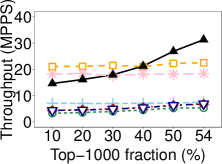
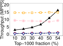
(a) 1D-byte	(b) 1D-bit

Figure 12: (Experiment 4) Throughput vs. skewness.

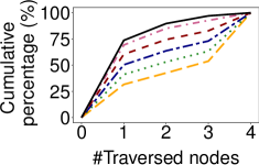
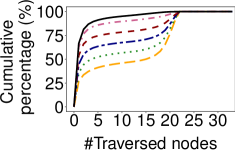
(a) 1D-byte	(b) 1D-bit

Figure 13: (Experiment 5) Number of traversed nodes.

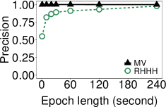
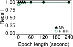
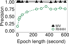
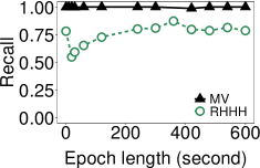
(a) Precision for 1D-byte	(b) Recall for 1D-byte	(c) Precision for 1D-bit	(d) Recall for 1D-bit

Figure 14: (Experiment 6) Convergence.

(Experiment 4) Throughput versus skewness.

While MVPipe is designed for highly skewed workloads, we evaluate the update throughput of MVPipe for less skewed workloads by varying the skewness degree of the CAIDA traces. In the original CAIDA traces used in our evaluation, the top-1000 flows account for 54% of the total number of packets in the traces. We vary the skewness degree of the traces by controlling the fraction of the total number of packets occupied by the top-1000 flows in each epoch. Specifically, we replace some packets of the top-1000 flows with new packets that have randomly generated source and destination IP addresses, such that the top-1000 flows account for a specified fraction (varied from 10% to 50%) of the total number of packets in each epoch. A smaller specified fraction implies a less skewed workload. Here, we set $w_{0}$ as 5,000 and 3,000 in 1D-byte and 1D-bit detection, respectively.

Figure 12 shows the update throughput of all schemes under various skewness degrees for 1D-byte and 1D-bit HHH detection. The throughput of MVPipe drops quickly as the specified fraction decreases (i.e., less skewed), as more packets need to be pushed to higher levels. Although MVPipe’s throughput decreases for less skewed workloads, its throughput remains higher than other schemes except for RHHH and TRIE.

(Experiment 5) Number of traversed nodes.

To understand the update throughput of MVPipe, we collect the number of nodes being traversed by MVPipe in a hierarchy for each packet update in both 1D-byte and 1D-bit hierarchies for different skewness degrees as specified in Experiment 4.

Figure 13 shows the cumulative percentage of packets versus the number of traversed nodes by MVPipe for different skewness degrees. We first examine the results for the original CAIDA traces (i.e., the top-1000 fraction is 54%). In 1D-byte HHH detection, 73% of packet updates traverse only one node in the hierarchy, where each packet update on average traverses only 1.39 nodes. In 1D-bit HHH detection, the number of traversed nodes slightly increases: only 66% of packet updates traverse one node, while each packet update on average traverses 2.36 nodes. The reason is that as the number of nodes increases in the 1D-bit hierarchy, each packet update generally needs to traverse more nodes in order to be admitted by a candidate HHH. Thus, MVPipe has lower throughput in 1D-bit HHH detection than in 1D-byte HHH detection. Nevertheless, since each packet update traverses only one node in a hierarchy in most cases, it justifies the high update throughput of MVPipe (see Figure 11 in Experiment 3).

We examine the results when the skewness degree decreases. As the top-1000 fraction decreases from 54% to 10%, the fraction of packet updates traversing only one node decreases from 73% to 31% for 1D-byte HHH detection, and from 66% to 26% for 1D-bit HHH detection. Correspondingly, the average number of traversed nodes per update increases from 1.39 to 2.72, and from 2.36 to 11.62, respectively. This explains the throughput drop of MVPipe for less skewed workloads.

(Experiment 6) Convergence.

We study the convergence by comparing the accuracy between MVPipe and RHHH [3] for various epoch lengths. We use the first twelve minutes of the CAIDA traces and vary the epoch length from one second to ten minutes (our default is one minute), where the number of packets in each epoch on average varies from 0.5 M to 401 M. For each epoch length, we divide the traces into multiple epochs (if the epoch length is larger than six minutes, we consider one epoch only). A small epoch length (e.g., one second) implies a small number of packets in the epoch, and any scheme that requires sufficient packets for convergence may have low accuracy. We set the absolute threshold for each epoch as $\phi\mathcal{S}$, where we fix $\phi=0.01$ and $\mathcal{S}$ as the total number of packets in that epoch. We keep the same memory usage of MVPipe and RHHH. We focus on 1D HHH detection, and similar observations are made for the 2D cases.

Figure 14 shows the results. The accuracy of RHHH drops in small epoch lengths, due to its slow convergence. For example, its precision is less than 0.9 if the epoch length is less than 30 s in the 1D-byte case; in the 1D-bit case, both its precision and recall converge to around 0.8 after 300 seconds (conforming to the results in the original paper [3]). In contrast, the precision and recall of MVPipe are higher than 0.99 in all settings.

(Experiment 7) MVPipe in hardware.

We evaluate MVPipe for 1D-byte HHH detection in a Tofino switch [36]. We configure the number of buckets from arrays $A_{0}$ to $A_{4}$ as 2048, 2048, 2048, 256, and 1, respectively. In this case, both the precision and recall of MVPipe are above 0.9 for an epoch length of one second in our traces.

Table I summarizes the resource usage of MVPipe in the Tofino switch, in terms of the number of physical stages used, SRAM consumption, the number of stateful ALUs consumed, and the message size overhead across stages in the packet header vector (PHV). MVPipe occupies all 12 physical stages of the switch. Nevertheless, its average resource consumption per stage is small, and the remaining resources in each occupied stage can still be made available for other applications. For example, MVPipe consumes only 2.81% of SRAM and 27.18% of stateful ALUs of the switch. The total size of messages across stages, including packet header information and metadata needed by MVPipe, is 132 bytes, among which only 48 bytes are due to the metadata from MVPipe.

We also validate that MVPipe’s throughput now achieves 100 Gb/s in our testbed (bounded by our packet generation rate), and it does not have any packet resubmission or recirculation. As MVPipe incurs limited switch resource overhead, we conjecture that its throughput in switch hardware can be even higher in production deployment.

No. stages	SRAM (KiB)	No. SALUs	PHV size (byte)
12 (100%)	432 (2.81%)	13 (27.08%)	132 (17.18%)

Table I: (Experiment 7) Switch resource usage of MVPipe; percentages are fractions of total resources.

VII Related Work

Dynamic data structures.

To maintain memory efficiency in HHH detection, prior studies propose dynamic data structures that insert or delete keys of interest on-the-fly. Trie-based HHH detection [39, 37] tracks keys in trie nodes and dynamically spawns new child nodes if a trie node has a byte count above a splitting threshold. Cormode et al. [11] propose full ancestry and partial ancestry, both of which build on Lossy Counting [22] with hierarchy awareness. Both algorithms maintain a lattice structure that dynamically adds or removes nodes. In contrast, MVPipe uses static memory allocation and incurs no dynamic memory management overhead.

Extensions of HH detection.

Several studies extend existing heavy-hitter-based solutions for HHH detection. Lin et al. [21] adapt Space Saving [23] to improve the accuracy of 1D HHH detection. Mitzenmacher et al. [24] further extend Space Saving with better space efficiency. Randomized HHH (RHHH) [3] extends the solution by Mitzenmacher et al. [24] with randomization: it maintains a Space Saving instance for each level of the hierarchy and randomly updates only one of the instances for each packet. While RHHH achieves high update throughput, it has slow convergence. In contrast, MVPipe preserves the invertibility and static memory allocation of MV-Sketch and adopts a pipelined design to achieve both lightweight updates and fast convergence in HHH detection.

TCAM-based solutions.

Some studies [17, 26, 30] leverage TCAM counters in hardware switches for 1D HHH detection, by matching and counting packets in the data plane and adapting the monitoring rules for different prefixes based on counter values. They rely on a centralized controller to decide the rules on which specific aggregation levels are monitored. In contrast, MVPipe can work entirely in the data plane for general aggregation levels.

Others.

Some HHH detection solutions specifically address the practical requirements of network measurement. AutoFocus [12] is an offline traffic analysis tool for identifying large traffic clusters. Cho [9] proposes a recursive partitioning approach for tractable HHH detection from an operational perspective.

VIII Conclusions

We revisit the HHH detection problem in network measurement. We present MVPipe, a novel invertible sketch that supports both lightweight updates and fast convergence in HHH detection and can be feasibly deployed in programmable switches. MVPipe builds on the skewness property of IP traffic and the pipelined executions of majority voting. Theoretical analysis and prototype evaluation in both software and hardware justify the design properties of MVPipe: high accuracy, high update throughput, fast convergence, and resource efficiency in P4-based switch deployment.

References

- [1] A. Appleby. https://github.com/aappleby/smhasher, 2016.
- [2] R. B. Basat, X. Chen, G. Einziger, and O. Rottenstreich. Designing Heavy-Hitter Detection Algorithms for Programmable Switches. IEEE/ACM Transactions on Networking, 2020.
- [3] R. B. Basat, G. Einziger, R. Friedman, M. C. Luizelli, and E. Waisbard. Constant Time Updates in Hierarchical Heavy Hitters. In Proc. of ACM SIGCOMM, pages 127–140, 2017.
- [4] R. Ben-Basat, X. Chen, G. Einziger, and O. Rottenstreich. Efficient Measurement on Programmable Switches Using Probabilistic Recirculation. In Proc. of IEEE ICNP, pages 313–323, 2018.
- [5] P. Bosshart, D. Daly, G. Gibb, M. Izzard, N. McKeown, J. Rexford, C. Schlesinger, D. Talayco, A. Vahdat, G. Varghese, et al. P4: Programming Protocol-Independent Packet Processors. ACM SIGCOMM Computer Communication Review, 44(3):87–95, 2014.
- [6] P. Bosshart, G. Gibb, H.-S. Kim, G. Varghese, N. McKeown, M. Izzard, F. Mujica, and M. Horowitz. Forwarding Metamorphosis: Fast Programmable Match-Action Processing in Hardware for SDN. In Proc. of ACM SIGCOMM, number 4, 2013.
- [7] R. S. Boyer and J. S. Moore. MJRTY – A Fast Majority Vote Algorithm. In Automated Reasoning, pages 105–117. Springer, 1991.
- [8] CAIDA. http://www.caida.org/data/passive/trace_stats/, 2022.
- [9] K. Cho. Recursive Lattice Search: Hierarchical Heavy Hitters Revisited. In Proc. of ACM IMC, pages 283–289, 2017.
- [10] K. Cho, K. Mitsuya, and A. Kato. Traffic Data Repository at the WIDE Project. In USENIX 2000 FREENIX Track, June 2000. https://mawi.wide.ad.jp/mawi/.
- [11] G. Cormode, F. Korn, S. Muthukrishnan, and D. Srivastava. Finding Hierarchical Heavy Hitters in Streaming Data. ACM Trans. on Knowledge Discovery from Data, 1(4):2, 2008.
- [12] C. Estan, S. Savage, and G. Varghese. Automatically Inferring Patterns of Resource Consumption in Network Traffic. In Proc. of ACM SIGCOMM, pages 137–148, 2003.
- [13] C. Estan and G. Varghese. New Directions in Traffic Measurement and Accounting. In Proc. of ACM SIGCOMM, 2002.
- [14] W. Fang and L. Peterson. Inter-AS Traffic Patterns and Their Implications. In Proc. of IEEE GLOBECOM, 1999.
- [15] S. K. Fayaz, Y. Tobioka, V. Sekar, and M. Bailey. Bohatei: Flexible and Elastic DDoS Defense. In Proc. of USENIX Security Symposium, pages 817–832, 2015.
- [16] A. Gupta, R. Harrison, M. Canini, N. Feamster, J. Rexford, and W. Willinger. Sonata: Query-Driven Streaming Network Telemetry. In Proc. of ACM SIGCOMM, pages 357–371, 2018.
- [17] L. Jose, M. Yu, and J. Rexford. Online Measurement of Large Traffic Aggregates on Commodity Switches. In Proc. of ACM Hot-ICE, 2011.
- [18] M. Kallitsis, S. A. Stoev, S. Bhattacharya, and G. Michailidis. AMON: An Open Source Architecture for Online Monitoring, Statistical Analysis, and Forensics of Multi-Gigabit Streams. IEEE Journal on Selected Areas in Communications, 34(6):1834–1848, 2016.
- [19] R. M. Karp, S. Shenker, and C. H. Papadimitriou. A Simple Algorithm for Finding Frequent Elements in Streams and Bags. ACM Trans. on Database Systems, 28(1):51–55, 2003.
- [20] J. Kučera, D. A. Popescu, H. Wang, A. Moore, J. Kořenek, and G. Antichi. Enabling Event-Triggered Data Plane Monitoring. In Proc. of ACM SOSR, pages 14–26, 2020.
- [21] Y. Lin and H. Liu. Separator: Sifting Hierarchical Heavy Hitters Accurately from Data Streams. Proc, of ACM ADMA, pages 170–182, 2007.
- [22] G. S. Manku and R. Motwani. Approximate Frequency Counts over Data Streams. In Proc. of ACM VLDB, pages 346–357, 2002.
- [23] A. Metwally, D. Agrawal, and A. E. Abbadi. Efficient Computation of Frequent and Top-K Elements in Data Streams. In Proc. of ICDT, pages 398–412, 2005.
- [24] M. Mitzenmacher, T. Steinke, and J. Thaler. Hierarchical Heavy Hitters with the Space Saving Algorithm. In Proc. of ACM ALENEX, pages 160–174, 2012.
- [25] J. Moraney and D. Raz. On the Practical Detection of Hierarchical Heavy Hitters. In Proc. of IFIP Networking, pages 37–45, 2020.
- [26] M. Moshref, M. Yu, and R. Govindan. Resource/Accuracy Tradeoffs in Software-Defined Measurement. In Proc. of ACM HotSDN, pages 73–78, 2013.
- [27] S. Narayana, A. Sivaraman, V. Nathan, P. Goyal, V. Arun, M. Alizadeh, V. Jeyakumar, and C. Kim. Language-Directed Hardware Design for Network Performance Monitoring. In Proc. of ACM SIGCOMM, pages 85–98, 2017.
- [28] P4 Open Source Programming Language. https://p4.org, 2022.
- [29] B. Pfaff, J. Pettit, T. Koponen, E. J. Jackson, A. Zhou, J. Rajahalme, J. Gross, A. Wang, J. Stringer, P. Shelar, et al. The Design and Implementation of Open vSwitch. In Proc. of USENIX NSDI, 2015.
- [30] D. A. Popescu, G. Antichi, and A. W. Moore. Enabling Fast Hierarchical Heavy Hitter Detection using Programmable Data Planes. In Proc. of ACM SOSR, pages 191–192, 2017.
- [31] N. Sarrar, S. Uhlig, A. Feldmann, R. Sherwood, and X. Huang. Leveraging Zipf’s Law for Traffic Offloading. ACM SIGCOMM Computer Communication Review, 42(1):16–22, 2012.
- [32] V. Sekar, N. Duffield, O. S. amd Kobus van der Merwe, and H. Zhang. LADS: Large-scale Automated DDoS Detection System. In Proc. of USENIX ATC, 2006.
- [33] A. Sivaraman, A. Cheung, M. Budiu, C. Kim, M. Alizadeh, H. Balakrishnan, G. Varghese, N. McKeown, and S. Licking. Packet Transactions: High-Level Programming for Line-Rate Switches. In Proc. of ACM SIGCOMM, pages 15–28, 2016.
- [34] V. Sivaraman, S. Narayana, O. Rottenstreich, S. Muthukrishnan, and J. Rexford. Heavy-Hitter Detection Entirely in the Data Plane. In Proc. of Proc. of SOSR, pages 164–176, 2017.
- [35] L. Tang, Q. Huang, and P. P. Lee. A Fast and Compact Invertible Sketch for Network-Wide Heavy Flow Detection. IEEE/ACM Trans. on Networking, 28(5):2350–2363, Oct 2020.
- [36] Tofino. https://www.intel.com/content/www/us/en/products/network-io/programmable-ethernet-switch/tofino-series/tofino.html, 2022.
- [37] P. Truong and F. Guillemin. Identification of Heavyweight Address Prefix Pairs in IP Traffic. In Proc. of IEEE International Teletraffic Congress, pages 1–8, 2009.
- [38] Y. Zhang, L. Breslau, V. Paxson, and S. Shenker. On the Characteristics and Origins of Internet Flow Rates. In Proc. of ACM SIGCOMM, 2002.
- [39] Y. Zhang, S. Singh, S. Sen, N. Duffield, and C. Lund. Online Identification of Hierarchical Heavy Hitters: Algorithms, Evaluation, and Applications. In Proc. of ACM IMC, pages 101–114, 2004.