One-Point Feedback for Composite Optimization with Applications to Distributed and Federated Learning

Abstract

This work is devoted to solving the composite optimization problem with the mixture oracle: for the smooth part of the problem, we have access to the gradient, and for the non-smooth part, only to the one-point zero-order oracle. For such a setup, we present a new method based on the sliding algorithm. Our method allows to separate the oracle complexities and compute the gradient for one of the function as rarely as possible. The paper also present the applicability of our new method to the problems of distributed optimization and federated learning. Experimental results confirm the theory.

1 Introduction

Composite optimization. In this paper, we focus on the composite optimization problem [34, 26]:

$$\min_{x\in\mathcal{X}}\Psi_{0}(x)\overset{\text{def}}{=}f(x)+g(x).$$ (1)

This problem occurs in a fairly large number of applications. In particular, we can recall the problems of minimizing the objective function $f(x)$ with regularization $g(x)$, which can often be found in machine learning [4]. Newer and more interesting applications of the composite problem arises in distributed optimization. In more detail, the goal of distributed optimization is to minimize the global objective function $f(x)=\frac{1}{M}\sum_{m=1}^{M}f_{m}(x)$, where functions $f_{1},\ldots,f_{M}$ are distributed among $M$ devices, and each device $m$ has access only to its local function $f_{m}$. Therefore, in order to solve this problem, one needs to establish a communication process between devices. Two methods are distinguished: centralized and decentralized. In a centralized case, all devices can only communicate with the central server – transfer information about the $f_{m}$ function to it and receive responses. In a decentralized case, there is no a central server; all devices are connected into a network, which can be represented as an undirected graph, where vertices are devices, and edges are the presence of a connection between a pair of devices. Communication in a decentralized network is typically done with the gossip protocol [24, 7, 32], which uses the so-called gossip matrix $W$. This matrix is built on the basis of the properties of the communication graph.

It turns out that distributed optimization problem can be written as a composite one [28, 17, 6, 12, 21, 20]:

$$\min_{X\in\mathcal{X}^{M}}\underbrace{\sum\limits_{m=1}^{M}f_{m}(x_{m})}_{f(X)}+\underbrace{\frac{\lambda}{M}\sum\limits_{m=1}^{M}\|x_{m}-\bar{x}\|^{2}_{2}}_{g(X)}$$ (2)

for the centralized case and

$$\min_{X\in\mathcal{X}^{M}}\underbrace{\sum\limits_{m=1}^{M}f_{m}(x_{m})}_{f(X)}+\underbrace{\lambda\|\sqrt{W}X\|^{2}_{2}}_{g(X)}$$ (3)

for decentralized one. Here we introduce the matrix $X=[x_{1},\ldots,x_{M}]^{T}$, the vector $\bar{x}=\frac{1}{M}\sum_{m=1}^{M}x_{m}$ and the parameter of regularization $\lambda>0$. The essence of expressions (2) and (3) is very simple. On each device, we have local variables $x_{m}$, and we penalize their deviations at the expense of the regularizer. In the centralized case, we penalize the deviation from the average across the entire network, and in the decentralized case, the difference between the connected devices (this is what the $W$ matrix is responsible for). In fact, in the decentralized case, we can also write the penalized problem in form (2). But if in case of a centralized architecture $\bar{x}$ is easy to calculate on the server, then in a decentralized network this is problematic (in particular, one of the devices have to be used as a server). Another important question is how to choose the $\lambda$ parameter. To get a close solution to the real solution of the distributed problem, one needs to take $\lambda$ large enough [12]. But more recently, problems (2) and (3) are considered from the point of view of personalized federated learning, in this case it makes sense to take small $\lambda$ as well [20, 21, 37].

Gradient-free methods. Now let us go back to the original problem (1). As noted above, the function $g$ often plays the role of a regularizer, usually it is a simple function for which the gradient $\nabla g$ can be computed . At the same time, the objective function $f$ can be quite complex. In this paper, we focus on the case when for the function $f$ only zero order oracle (i.e., only the values of the function $f$, but not its gradient) is available. In the literature, this concept is sometimes referred to as a black-box. It arises when the calculation of gradient is expensive (in Adversarial training [9], optimization [35], structured-prediction [41]) or impossible (in Reinforcement learning [15, 10, 38], bandit problem [8, 39], black box ensemble learning [29]). To make the problem statement even more practical we assume that we have access inexact values of function $f(x,\xi)$ with some random noise $\xi$. With the help of this oracle, it is possible to make some approximation of the gradient in terms of finite differences. Next we highlight two main approaches for such gradient estimates. The first approach is called a two-point feedback:

$$\tilde{f}^{\prime}_{r}(x,\xi)\overset{\text{def}}{=}\frac{n}{2r}(f(x+re,\xi)-f(x-re,\xi))e,$$ (4)

where $e$ is uniformly distributed on the unit euclidean sphere. For two-point feedback there are a lot of papers with theoretical analysis [11, 35, 16, 39, 14, 18]. An important thing of this approach is the assumption that we were able to obtain the values of the function in points $x+re$ and $x-re$ with the same realization of the noise $\xi$. But from a practical point of view, this is a very strong and idealistic assumption. Therefore, it is proposed to consider the concept of one-point feedback [16, 1, 36]:

$$\tilde{f}^{\prime}_{r}(x,\xi^{\pm})\overset{\text{def}}{=}\frac{n}{2r}(f(x+re,\xi^{+})-f(x-re,\xi^{-}))e.$$ (5)

In general $\xi^{+}\neq\xi^{-}$. In this paper we work with one-point concept.

The function $f$ is ”bad”, while the function $g$ is ”good”. The question arises how to minimize $\Psi_{0}$ from (1). The easiest option is to add the gradient $g$ and the ”gradient” $f$ (from (5)) and make step along it. In this approach, there are no problems when $g$ is just a Tikhonov regularizer, but if we look at problems (2) and (3), to compute the gradient of $g$ we need to make communication, while to calculate the ”gradient” $f$ we do not need it. But communications are the bottleneck of distributed algorithms, they require significantly more time than local computations. Therefore, one wants to reduce the number of communications and to calculate the gradient $g$ as rarely as possible.

This brings us to the goal of this paper: to come up with an algorithm that solves the composite optimization problem for one part of which we have a one-point zero order oracle, and for the other – a gradient. At the same time, we want to call this gradient as rarely as possible.

1.1 Our contribution

We present a new method based on the sliding technique for the convex problem (1) with the mixture oracle: first order for the smooth part $g$ and zeroth order for the non-smooth part $f$. Our method solves the problems mentioned above in the introduction. It reduces the number of calls for the gradient $\nabla g$ of the smooth part of the composite problem, while using one-point feedback for the non-smooth part $f$.

Note that all the results were obtain in general (non-euclidean) proximal setup. This allows sometimes to reduce $f$-oracle calls complexity $\sim n$-times in comparison with algorithms that use euclidean setup, where $n$ is a dimension of the problem – see Table 1.

	$\|\cdot\|=\|\cdot\|_{2}$	$\|\cdot\|=\|\cdot\|_{1}$
$\nabla g$	$O\left(\sqrt{\frac{LD^{2}}{\varepsilon}}\right)$	$O\left(\sqrt{\frac{LD^{2}}{\varepsilon}}\right)$
$f$	$\tilde{O}\left(\sqrt{\frac{LD^{2}}{\varepsilon}}+\frac{nG^{2}D^{2}}{\varepsilon^{2}}+\frac{n^{2}G^{2}\sigma^{2}D^{2}}{\varepsilon^{4}}\right)$	$O\left(\sqrt{\frac{LD^{2}}{\varepsilon}}+\frac{\ln nG^{2}D^{2}}{\varepsilon^{2}}+\frac{n\ln nG^{2}\sigma^{2}D^{2}}{\varepsilon^{4}}\right)$

Table 1: Summary of complexity results on the number of $\nabla g$ and $f$ calls for finding an $\varepsilon$-solution of (1) in the different geometric setups: Euclidean and non-Euclidean. Convergence is measured by the function distance to the solution. Notation: $L$ = constant of $L$-smoothness of $g$ (in the corresponding norm), $G$ = bound of $\nabla f$ (only for theory), $n$ = dimension of vector $x$ ($\mathcal{X}\subset\mathbb{R}^{n}$), $\sigma^{2}$ = variance of unbiased noise $\xi$, $D$ = diameter of $\mathcal{X}$(in the corresponding geometry).

We also present the applicability and relevance of our new method for distributed and federated learning problems in both centralized (2) and decentralized (3) setups – see Table 2. It turns out that this method can be useful in terms of reducing the number of communications.

	Centralized	Decentralized
comm	$O\left(\sqrt{\frac{\lambda D^{2}}{\varepsilon}}\right)$	$O\left(\sqrt{\frac{\lambda\lambda_{\max}(W)D^{2}}{\varepsilon}}\right)$
local	$O\left(\sqrt{\frac{\lambda D^{2}}{\varepsilon}}+\frac{nG^{2}D^{2}}{\varepsilon^{2}}+\frac{n^{2}G^{2}\sigma^{2}D^{2}}{\varepsilon^{4}}\right)$	$O\left(\sqrt{\frac{\lambda\lambda_{\max}(W)D^{2}}{\varepsilon}}+\frac{nG^{2}D^{2}}{\varepsilon^{2}}+\frac{n^{2}G^{2}\sigma^{2}D^{2}}{\varepsilon^{4}}\right)$

Table 2: Summary of complexity results on communications (comm) and local computations (local) for finding an $\varepsilon$-solution of centralized (2) and decentralized (3) distributed problems. Convergence is measured by the function distance to the solution. Notation: $\lambda_{\max}(W)$ = maximum eigenvalue of $W$, $G$ = bound of $\nabla f$ (only for theory), $n$ = dimension of vector $x$ ($\mathcal{X}\subset\mathbb{R}^{n}$), $\sigma^{2}$ = variance of unbiased noise $\xi$, $D$ = diameter of $\mathcal{X}$ (in the Euclidean norm).

1.2 Comparison with known results

Let us note some works related to our paper.

Sliding. The naive approach to (1) looks at it as a whole problem and not take into account its composite structure. This can significantly worsen the oracle complexities for one of the functions. Sliding technique allows to avoid those losses and to separate oracle complexities. In particular, if we can solve a separate problem $\min f(x)$ by $T_{f}$ oracle calls (these can be calls of gradient or any other oracle, for example, zeroth order), and a problem $\min g(x)$ by $T_{g}$ oracle calls, then sliding techniques gives that we can solve the composite problem by $\mathcal{O}(T_{f})$ oracle calls corresponds to $f$ and $\mathcal{O}(T_{g})$ oracle calls corresponds to $g$. If we use naive approach we have the same complexities $\mathcal{O}(\max(T_{g};T_{f}))$ for both $f$ and $g$.

There are various types of sliding in the literature, depending on what assumptions are made for (1).

• Sliding was justified for smooth $f$ and $g$ with gradient oracles for convex optimization problems in [23, 3, 42, 27, 30].

• In [13, 22] they considered case with smooth $f$ and smooth $g$ with zeroth-order oracle for $f$ and gradient oracle for $g$.

• In [25, 26] Sliding was used for non-smooth $f$ and smooth $g$ with stochastic subgradient oracle for $f$ and gradient oracle for $g$.

• Based on [25] in [6] Sliding was adapted for non-smooth $f$ and smooth $g$ with two-point zeroth-order stochastic oracle (4) for $f$ and gradient oracle for $g$.

The development of sliding technique is a quite popular issue in the literature, but on the other hand it should be mentioned that there are still a lot of open problems especially for mixture oracle. In this paper we concentrated on generalization of [6] for non-smooth $f$ and smooth $g$ with one-point zeroth-order stochastic oracle for $f$ ((5) feedback rather than (4) of [6]) and gradient oracle for $g$ for convex optimization problems. For strongly convex problems our results can also be generalized by using standard restart technique, see i.e. [6].

Gradient-free methods. Let us highlight the main works devoted to the zeroth-order methods: for two-point feedback [40, 35, 11, 16, 39, 14, 18], for one-point feedback [5, 16, 1, 36]. For two-point stochastic/deterministic feedback optimal methods for smooth/non-smooth, convex/strongly convex problems were developed in cited papers. For one-point problem there are still a gap between lower bounds and complexities of the best known methods. In this paper we generalize the best-known composite-free ($g=0$) results concerning non-smooth $f$ with stochastic one-point feedback from [16] for smooth $g\neq 0$ with gradient oracle.

Distributed setup. For (strongly) convex optimization problems optimal (stochastic) gradient decentralized method have been developed – see surveys [12, 19] and references therein. For stochastic two-point feedback (with non-smooth target function $f$) optimal decentralized methods were developed in [6]. To the best of our knowledge this is the only optimal result in this field. For one-point stochastic feedback we know only one result [2], they assume that target function $f$ is highly-smooth and strongly convex. Their result is best known for one-point stochastic feedback oracle, but the method is very expensive in terms of decentralized communication. The reason is that in [2] authors fight only for oracle calls criteria and do not use Sliding technique that allows to split communication complexity from the oracle one. In our paper by using Sliding technique we split these complexities in reduced problem (3) and obtain much better communication complexity.

2 Preliminaries

First, we define several notation. We denoted the inner product of $x,y\in\mathbb{R}^{n}$ as $\langle x,y\rangle\overset{\text{def}}{=}\sum_{i=1}^{n}x_{i}y_{i}$, where $x_{i}$ corresponds to the $i$-th component of $x$ in the standard basis in $\mathbb{R}^{n}$. Also, we denote $\ell_{p}$-norms as $\|x\|_{p}\overset{\text{def}}{=}\left(\sum_{i=1}^{n}|x_{i}|^{p}\right)^{\frac{1}{p}}$ for $p\in(1,\infty)$ and for $p=\infty$ we use $\|x\|_{\infty}\overset{\text{def}}{=}\max_{1\leq i\leq n}|x_{i}|$ And for the dual norm $\|\cdot\|_{*}$ for the norm $\|\cdot\|$ is defined in the following way: $\|y\|_{*}\overset{\text{def}}{=}\max\left\{\langle x,y\rangle\mid\|x\|\leq 1\right\}$. Operator $\mathbb{E}[\cdot]$ denotes full mathematical expectation and operator $\mathbb{E}_{\xi}[\cdot]$ express conditional mathematical expectation w.r.t. all randomness coming from random variable $\xi$.

Now let us introduce a few definitions

Definition 2.1 ($L$-smoothness).

Function $g$ is called $L$-smooth in $X\subseteq\mathbb{R}^{n}$ with $L>0$ w.r.t. norm $\|\cdot\|$ when it is differentiable and its gradient is $L$-Lipschitz continuous in $X$, i.e.

$$\|\nabla g(x)-\nabla g(y)\|_{*}\leq L\|x-y\|,\quad\forall x,y\in X.$$

One can show that $L$-smoothness implies [34]

$$g(x)\leq g(y)+\langle\nabla g(y),x-y\rangle+\dfrac{L}{2}\|x-y\|^{2},\quad\forall x,y\in X.$$ (6)

Definition 2.2 (Bregman divergence).

Assume that function $\nu(x)$ is $1$-strongly convex w.r.t. $\|\cdot\|$-norm and differentiable on $X$ function. Then for any two points $x,y\in X$ we define Bregman divergence $V(x,y)$ associated with $\nu(x)$ as follows:

$$V(x,y)\overset{\text{def}}{=}\nu(y)-\nu(x)-\langle\nabla\nu(x),y-x\rangle.$$

Then we denote the Bregman-diameter of the set $X$ w.r.t. $V(x,y)$ as $D_{X,V}\overset{\text{def}}{=}\max\{\sqrt{2V(x,y)}\mid x,y\in X\}$.

Definition 2.3 (convex function).

Continuously differentiable function $g(x)$ is called convex in $\mathbb{R}^{n}$ if the inequality holds for $x,y\in\mathbb{R}^{n}$ any

$$g(y)\geq g(x)+\langle\nabla g(x),y-x\rangle.$$ (7)

3 Main part

Recall that we consider the composite optimization problem (1). To take into account the ”geometry” of the problem, we work in a certain (not necessarily Euclidean) norm $\|\cdot\|$ (with dual norm $\|\cdot\|_{*}=\|\cdot\|_{q}$), and also measure the distance using the Bregman divergence $V$. Assume that $X\subseteq\mathbb{R}^{n}$ is a compact and convex set with diameter $D_{X,V}$, function $g$ is convex and $L$-smooth w.r.t. $\|\cdot\|$-norm on $X$, function $f$ is convex differentiable function on $X$. Assume we can use the first-order oracle for $g(x)$ and zeroth-order oracle with in unbiased stochastic noise for $f(x)$, i.e. we have access to

$$\tilde{f}(x,\xi)\overset{\text{def}}{=}f(x)+\xi$$ (8)

where $\xi$ is generated randomly regardless of the point $x$. Additionally, we assume that the noise is bounded:

$$\mathbb{E}\xi=0,\quad\mathbb{E}[\xi^{2}]\leq\sigma^{2}.$$ (9)

Also assume that for all $x\in X$

$$\|\nabla f(x)\|_{2}\leq G.$$ (10)

Note that the boundedness of the (sub-)gradient $f$ is needed only for the theoretical analysis; in practice, the method uses only the oracle with the values of the function.

3.1 From first to zeroth order

Before presenting the main Algorithm, let us understand the properties of the approximation (5) that we use. Most of these properties have already been encountered in the literature [39], we modified only a few of them for our case. These properties are associated with the next object

$$F(x)\overset{\text{def}}{=}\mathbb{E}[f(x+re)].$$ (11)

The function $F$ is called the ”smoothed” version of the function $f$. Our algorithm does not use it in any way, but it will be used in the theoretical analysis.

Lemma 3.1 (see Lemmas 1 and 2 from [6]).

$F(x)$ is convex, differentiable and it holds that

$$\sup_{x\in X}|F(x)-f(x)| \leq rG,$$ (12)

$$\mathbb{E}[\tilde{f}^{\prime}_{r}(x,\xi^{\pm})]-\nabla F(x) =0,$$ (13)

$$\mathbb{E}[\|\tilde{f}^{\prime}_{r}(x,\xi^{\pm})\|^{2}_{*}] \leq p^{2}(n)\left(3nG^{2}+\frac{2n^{2}\sigma^{2}}{r^{2}}\right),$$ (14)

where $p^{2}(n)\overset{\text{def}}{=}\min\{2q-1,32\log n-8\}n^{\frac{2}{q}-1}$.

Let us discuss these facts. The property (28) gives that approximation (5) is an unbiased estimation of the gradient, not of the original function $f$, but of the smoothed function $F$. This means that we can replace the original problem (1) with $\min[F(x)+g(x)]$ and now consider the oracle (5) for $F$ as an unbiased stochastic gradient with a second moment equal to (29). The question arises how much the new problem differs from the original one? (12) says that for a small parameter $r$ the original problem (1) and the new one are very close. The proof of the algorithm will be built on this idea.

3.2 Algorithm

As mentioned above, our algorithm is based on the sliding algorithm [25, 6]. Our algorithm is a modification of the first order sliding with a zeroth order oracle. Sliding (complexities splitting) effect is achieved due to the fact that the method consists of an outer and inner loops. At the outer iterations, we calculate the gradient of the function $g$, while at the inner loop (prox-sliding procedure), only the function $f$ is used, with fixed information about the gradient $g$.

Algorithm 1 One-Point Zeroth-Order Sliding Algorithm (OPZOSA)

1:Initial point $x_{0}\in X$ and iteration limit $N$. Let $\beta_{k}\in\mathbb{R}_{++}$, $\gamma_{k}\in\mathbb{R}_{+}$, and $T_{k}\in\mathbb{N}$, $k=1,2,...$, be given and set $\overline{x}_{0}=x_{0}$.

2:for $k=1,...,N$ do

3:     Set $\underline{x}_{k}=(1-\gamma_{k})\overline{x}_{k-1}+\gamma_{k}x_{k-1}$ and let $h_{k}(y)=g(x_{k})+\left<\nabla g(x_{k}),y-x_{k}\right>$

4:     Set $(x_{k},\tilde{x}_{k})=\text{{\tt PS}}(h_{k},x_{k-1},\beta_{k},T_{k})$

5:     Set $\overline{x}_{k}=(1-\gamma_{k})\overline{x}_{k-1}+\gamma_{k}\tilde{x}_{k}$

6:end for

7:Result: $\overline{x}_{N}$

The PS procedure: $(x^{+},\tilde{x}^{+})=\text{{\tt PS}}(h,x,\beta,T)$

1:Let the parameters $p_{t}\in\mathbb{R}_{++}$ and $\theta_{t}\in[0,1],t=1,...$ be given. Set $u_{0}=\tilde{u}_{0}=x$.

2:for $t=1,...,T$ do

3:     $u_{t}=\mathop{\arg\!\min}\limits_{u\in X}\left\{h(u)+\left<\tilde{f^{\prime}_{r}}(u_{t-1},\xi^{\pm}_{t-1}),u\right>+\beta V(x,u)+\beta p_{t}V(u_{t-1},u)\right\}$

4:     $\tilde{u}_{t}=(1-\theta_{t})\tilde{u}_{t-1}+\theta_{t}u_{t}$

5:end for

6:Set $x^{+}=u_{T}$ and $\tilde{x}^{+}=\tilde{u}_{T}$.

The following theorem gives an estimate for the convergence of this method:

Theorem 3.2.

Suppose that $p_{t}=\frac{t}{2}$, $\theta_{t}=\frac{2(t+1)}{t(t+3)}$, $\beta_{k}=\frac{2L}{k}$, $\gamma_{k}=\frac{2}{k+1}$,

$$T_{k}=\max\left\{1;\frac{16Nk^{2}}{3D_{X,V}^{2}L^{2}}\cdot\left(14p^{2}(n)nG+\frac{p^{2}(n)n^{2}\sigma^{2}}{r^{2}}\right)\right\}$$

for $t\geq 1,k\geq 1$. Then for any number of iteration $N$ it holds that

$$\mathbb{E}[\Psi_{0}(\overline{x}_{N})-\Psi_{0}(x^{*})] \leq 2rG+\frac{12LD_{X,V}^{2}}{N(N+1)}.$$ (15)

Additionally, the total number of PS procedure iteration is

$$T^{\text{total}}=\frac{(N+1)^{4}}{D_{X,V}^{2}L^{2}}\cdot\left(14p^{2}(n)nG+\frac{p^{2}(n)n^{2}\sigma^{2}}{r^{2}}\right).$$ (16)

This Theorem shows the significance of the choice of $r$. In particular, it follows from (59) that $r$ should be taken as small as possible. On the other hand, it follows from (16) that as $r$ decreases, the total number of internal iterations increases. From here we get a game to some extent: the parameter $r$ must be controlled and adjusted carefully.

Corollary 3.3.

Under assumptions of Theorem 3.2 and if we put $r=\Theta\left(\frac{\varepsilon}{G}\right)$, then the number of calling for $\nabla g$ and $f$ required by Algorithm 1 to find an $\varepsilon$-solution $\overline{x}_{N}$ of (1) that $\mathbb{E}[\Psi_{0}(\overline{x}_{N})]-\Psi_{0}(x^{*})\leq\varepsilon$, is bounded by

$$O\left(\sqrt{\frac{LD_{X,V}^{2}}{\varepsilon}}\right)\quad\text{and}$$

$$O\left(\sqrt{\frac{LD_{X,V}^{2}}{\varepsilon}}+\frac{n\cdot p^{2}(n)G^{2}D_{X,V}^{2}}{\varepsilon^{2}}+\frac{n^{2}\cdot p^{2}(n)G^{2}\sigma^{2}D_{X,V}^{2}}{\varepsilon^{4}}\right).$$

This is the result that we wanted to achieve in the use of Sliding. The oracle complexity for $\nabla g$ was not affected in any way by the fact that we use a ”very bad” oracle for $f$. Our results also cover those obtained for one-point feedback in the non-distributed composite-free case [16].

Remark. Note that the second estimate depends on the ”geometry” of the problem. In particular, in the Euclidean case $q=2$ and then we have the following oracle complexity for $f$

$$O\left(\sqrt{\frac{LD_{X}^{2}}{\varepsilon}}+\frac{nG^{2}D_{X}^{2}}{\varepsilon^{2}}+\frac{n^{2}G^{2}\sigma^{2}D_{X}^{2}}{\varepsilon^{4}}\right).$$ (17)

A more interesting case is the case when we work in the non-Euclidean setting (for example, on a probability simplex), then $\|\cdot\|=\|\cdot\|_{1}$ and $q=\infty$ and $D_{X,V}^{2}=2\ln n$, in this case the estimate is transformed into

$$O\left(\sqrt{\frac{LD_{X,V}^{2}}{\varepsilon}}+\frac{\ln n\cdot G^{2}D_{X,V}^{2}}{\varepsilon^{2}}+\frac{n\ln n\cdot G^{2}\sigma^{2}D_{X,V}^{2}}{\varepsilon^{4}}\right).$$ (18)

It can be seen that (18) improves the estimate (17) $n$ times by using a different geometric setup. Moreover, if the noise $\sigma=0$, our estimates are the same (up to $\ln n$) with the estimates for the full-gradient method [25].

3.3 Applications to distributed optimization

Now let us move on to some examples, including those for which sliding gives the estimates necessary from practice. We consider problems (2) and (3). We briefly mentioned in the introduction that in these problems, we need to reduce the number of $\nabla g$ calls, thereby reducing the number of communications. Indeed, in order to calculate the gradient $g$ in the problem (2), we need to know the value of $\bar{x}$. But there is no way to calculate this only with the help of local computations, which means that one need help of the central server: send all current $x_{m}$ and get the average $\bar{x}$. At the same time, any calculations of $f$ do not require communications. To compute $f(X)$ we need to compute $f_{m}(x_{m})$, and this is just the values of local functions on local variables. For problem (3), the same reasoning is valid, but communication takes place with neighbors using the gossip protocol with $W$.

Then we a ready to obtain estimates for problems (2) and (3) from the general results of the previous section. We consider the Euclidean case. Let assume that all functions $f_{m}$ have bounded gradient with constant $G$. Then $f(X)$ has also bounded gradient. One can note that $g$ is $\lambda$-smooth in (2) and $\lambda\lambda_{\max}(W)$-smooth in (3). Recall that the number of the computations of $\nabla g(X)$ corresponds to the number of the communication rounds, and the calls $f(X)$ – to the local gradient-free calculations. Then the following estimates are valid for the number of communications and local iterations:

• in the centralized case

  $$O\left(\sqrt{\frac{\lambda D_{X,V}^{2}}{\varepsilon}}\right)\quad\text{communication rounds}\quad\text{and}$$

  $$O\left(\sqrt{\frac{\lambda D_{X,V}^{2}}{\varepsilon}}+\frac{nG^{2}D_{X,V}^{2}}{\varepsilon^{2}}+\frac{n^{2}G^{2}\sigma^{2}D_{X,V}^{2}}{\varepsilon^{4}}\right)\quad\text{local computations;}$$

• and in the decentralized case

  $$O\left(\sqrt{\frac{\lambda\lambda_{\max}(W)D_{X,V}^{2}}{\varepsilon}}\right)\quad\text{communication rounds}\quad\text{and}$$

  $$O\left(\sqrt{\frac{\lambda\lambda_{\max}(W)D_{X,V}^{2}}{\varepsilon}}+\frac{nG^{2}D_{X,V}^{2}}{\varepsilon^{2}}+\frac{n^{2}G^{2}\sigma^{2}D_{X,V}^{2}}{\varepsilon^{4}}\right)\quad\text{local computations.}$$

This is a rather remarkable result. We have ”very bad” local functions (they are non-smooth and only with the zeroth order information), but this fact does not reflect dramatically on communications. It remains only to discuss the selection of $\lambda$ parameter for problems (2) and (3). In fact, this is a key in personalized learning to select of $\lambda$ parameter: a small $\lambda$ parameter is a small regularizer, and then a small penalty for the fact that all local variables are not similar to each other, then each $x_{m}$ takes a little information from others $x$ and rely primarily on the local function $f_{m}$. The reverse situation is observed with a large $\lambda$. All $x_{m}$ tend to the same value. In particular, there are two extreme cases:

• If $\lambda=0$, then (2) and (3) becomes

  $$\min_{X\in\mathcal{X}^{M}}\sum^{M}_{m=1}f_{m}(x_{m}).$$

  This is equivalent to independent local optimization without communications.

• As $\lambda\to+\infty$, (2) and (3) tends to the distributed problem with equal local arguments

  $$\min_{x_{1}=\dots=x_{M}\in\mathcal{X}}\sum^{M}_{m=1}f_{m}(x_{m}).$$

  Note that an infinite $\lambda$ can mess up estimates on communications. It turns out $\lambda$ can be taken large but not infinite [12, 6]. In particular, it is enough to take $\lambda=\frac{G^{2}}{\lambda^{+}_{\min}(W)\varepsilon}$. And then we have the following communication complexities:

  $$O\left(\frac{GD_{X,V}}{\varepsilon}\right),\quad O\left(\sqrt{\chi}\frac{GD_{X,V}}{\varepsilon}\right)$$

  in the centralized and decentralized cases, respectively.

4 Experiments

The purpose of our experiments is to compare how our method works in practice in comparison with classical methods. In particular, we compare our method with methods that do not take into account the composite structure of the problem (1). As such a method, we consider Mirror Descent in two settings: in the first case, we consider full-gradient mirror descent [33], which uses $\nabla f+\nabla g$ as a gradient; we also consider a gradient-free version of it, which uses $\tilde{f}^{\prime}_{r}(x,\xi^{\pm})+\nabla g$ as a ”gradient”.

Comparison is made up on the problem of distributed computation of geometric median [31, 6]. We have $m$ vectors $b_{1},\ldots,b_{m}\in\mathbb{R}^{n}$:

$$\min\limits_{x\in\mathbb{R}^{n}}f(x)=\sum\limits_{m=1}^{M}\|x-b_{m}\|_{2}.$$

We distributed vectors $b$ among 10 computing devices. Then the problem can be written in the form (3):

$$\min\limits_{X\in\mathbb{R}^{n\times M}}\underbrace{\sum\limits_{m=1}^{M}\overbrace{\|x_{m}-b_{m}\|_{2}}^{f_{m}(x_{m})}}_{f(X)}+\underbrace{\frac{\lambda}{2}\|\sqrt{W}\mathbf{x}\|_{2}^{2}}_{g(X)}.$$ (19)

To make our problem stochastic. Each time when we compute $\nabla f$ or the value $f$, we generate a small normal noise vector $\xi_{m}$ for each vector $b_{m}$.

We run Algorithm 1, the first order Mirror Descent [33] and the zeroth order Mirror Descent [11] on problem (19) with $n=100$, $M=50$ and $\lambda=10^{2}$. Vectors $b_{1},\ldots,b_{m}$ are generated as i.i.d. samples from normal distributed ${\cal N}({\mathbf{1}},2I_{n})$, noise $\xi$ is also generated from normal distributed ${\cal N}(0,\sigma^{2}I_{n})$, where $\sigma=0,01$. We consider different decentralised topologies: star, cycle, chain, i.e. path, and complete graph. All methods tuned for better convergence: in the first order Mirror Descent we tune step size, in the zeroth order Mirror Descent we put $r=10^{-2}$ in (5) and also tune step size, Algorithm 1 is not tuned and is used with theoretical set of parameters from Theorem 3.2 and $r=10^{-2}$ in (5). The main comparison criterion is the number of communications, i.e. calls to the oracle $\nabla g=\lambda WX$. See Figure 1 for results. We notice that in these tests Algorithm 1 outperforms even Mirror Descent which is a first-order method. This shows the importance of taking into account the composite structure of the problem.

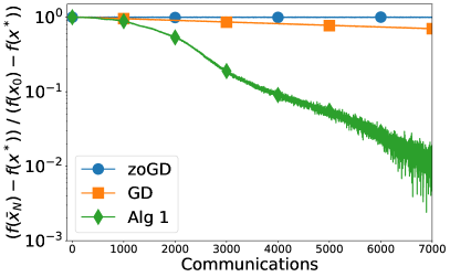
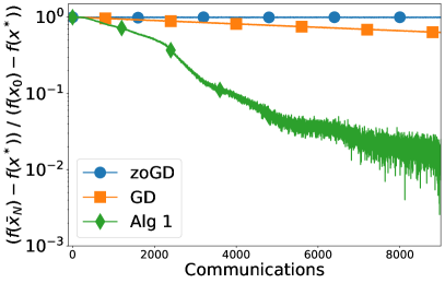
(a) star

(b) complete

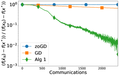
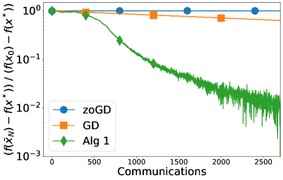
(c) chain

(d) cycle

Figure 1: Algorithm 1 (green), first order Mirror Descent (blue) and zeroth order Mirror Descent (orange) applied to solve (19) for different network topologies.

Supplementary Material

Appendix A Basic Facts

Lemma A.1.

For arbitrary integer $n\geq 1$ and arbitrary set of positive numbers $a_{1},\ldots,a_{n}$ we have

$$\left(\sum\limits_{i=1}^{m}a_{i}\right)^{2}\leq m\sum\limits_{i=1}^{m}a_{i}^{2}$$ (20)

Lemma A.2 (Hölder inequality).

For arbitrary $x,y\in\mathbb{R}^{n}$ the following inequality holds

$$\langle x,y\rangle\leq\|x\|_{*}\cdot\|y\|$$ (21)

Lemma A.3 (Cauchy-Schwarz inequality for random variables.).

Let $\xi$ and $\eta$ be real valued random variables such that $\mathbb{E}[\xi^{2}]<\infty$ and $\mathbb{E}[\eta^{2}]<\infty$. Then

$$\mathbb{E}[\xi\eta]\leq\sqrt{\mathbb{E}[\xi^{2}]\mathbb{E}[\eta^{2}]}.$$ (22)

Lemma A.4 (Strong convexity of Bregman divergence.).

For any points $x,y\in X$ the following inequality holds

$$V(x,y)\geq\frac{1}{2}\|x-y\|^{2}.$$ (23)

Appendix B Auxiliary Results

Lemma B.1 (Lemma 9 from [40]).

For any function $g$ which is $M$-Lipschitz with respect to the $\ell_{2}$-norm, it holds that if $e$ is uniformly distributed on the Euclidean unit sphere, then

$$\sqrt{\mathbb{E}[(g(e)-\mathbb{E}g(e))^{4}]}\leq\frac{4M^{2}}{n}.$$

Lemma B.2 (Lemma 3.5 from [26]).

Let the convex function $p:X\to\mathbb{R}$, the points $\tilde{x},\tilde{y}\in X$ and scalars $\mu_{1},\mu_{2}\geq 0$ be given. Let $\nu:X\to\mathbb{R}$ be a differentiable convex function and $V(x,z)$:

$$V(x,z)=\nu(z)-[\nu(x)+\nabla\nu(x)^{\top}(z-x)].$$

If

$$\tilde{u}=\mathop{\arg\!\min}_{u\in X}\{p(u)+\mu_{1}V(\tilde{x},u)+\mu_{2}V(\tilde{y},u)\},$$

then for any $u\in X$, we have

$$p(\tilde{u})+\mu_{1}V(\tilde{x},\tilde{u})+\mu_{2}V(\tilde{y},\tilde{u})\leq p(u)+\mu_{1}V(\tilde{x},u)+\mu_{2}V(\tilde{y},u)-(\mu_{1}+\mu_{2})V(\tilde{u},u).$$

Lemma B.3 (Lemma 3.17 from [26]).

Let $w_{k}\in(0;1]$, $k=1,2,\ldots$ be given. Also let us denote

$$W_{k}=\begin{cases}1,&k=1,\\ (1-w_{k})W_{k-1},&k>1.\end{cases}$$

Suppose that $W_{k}>0$ for all $k>1$ and that the sequence $\{\Delta_{k}\}_{k\geq 0}$ satisfies

$$\Delta_{k}\leq(1-w_{k})\Delta_{k-1}+B_{k},~{}~{}~{}k=1,2,\ldots$$

for some positive constants $\{B_{k}\}_{k\geq 0}$. Then, we have

$$\Delta_{k}\leq W_{k}(1-w_{1})\Delta_{0}+W_{k}\sum\limits_{i=1}^{k}\frac{B_{i}}{W_{i}}.$$

Lemma B.4.

Assume that for the differentiable function $f$ defined on a closed and convex set $X$ there exists such $M$ that

$$\|\nabla f(x)\|_{*}\leq G\quad\forall x\in X.$$ (24)

Then,

$$f(x)\leq f(y)+\langle\nabla f(y),x-y\rangle+2G\|x-y\|,\quad\forall x,y\in X.$$

Proof of Lemma B.4. For arbitrary points $x,y\in X$ we have

$$f(x) =f(y)+\int\limits_{0}^{1}\langle\nabla f(y+\tau(x-y)),x-y\rangle d\tau$$

$$=f(y)+\langle\nabla f(y),x-y\rangle+\int\limits_{0}^{1}\langle\nabla f(y+\tau(x-y))-\nabla f(y),x-y\rangle d\tau.$$

Using (21) and then (24), we obtain

$$f(x) \overset{}{\leq}f(y)+\langle\nabla f(y),x-y\rangle+\int\limits_{0}^{1}\|\nabla f(y+\tau(x-y))-\nabla f(y)\|_{*}\cdot\|x-y\|d\tau$$

$$\overset{}{\leq}f(y)+\langle\nabla f(y),x-y\rangle+\int\limits_{0}^{1}2G\|x-y\|d\tau$$

$$\leq f(y)+\langle\nabla f(y),x-y\rangle+2G\|x-y\|.$$

Appendix C Proof of Lemma 3.1

In this Section, we prove Lemma 3.1. For convenience, we divided the proof into two lemmas. Lemma C.1 gives the properties of the function (11), and Lemma C.2 – the properties of the approximation (5). Also, for convenience, we duplicate the statements of Lemma 3.1.

Lemma C.1 (Lemma 8 from [39] and Lemma 1 from [6]).

$F(x)$ defined in (11) is convex, differentiable and $F(x)$ satisfies

$$\nabla F(x) =\mathbb{E}\left[\frac{n}{r}f(x+re)e\right],$$ (25)

$$\sup_{x\in X}|F(x)-f(x)| \leq rG,$$ (26)

$$\|\nabla F(x)\|_{*} \leq 2\sqrt{n}p(n)G,$$ (27)

where $p^{2}(n)$ defined as follows: $\sqrt{\mathbb{E}[\|e\|_{*}^{4}]}\leq p^{2}(n)\overset{\text{def}}{=}\min\{2q-1,32\log n-8\}n^{\frac{2}{q}-1})$.

Proof of Lemma C.1: The convexity and differentiability of the function $F(x)$ and (25) follows from Lemma 8 of [39]. Then using sequentially the definition of $F(x)$ and the properties of the expectation associated with the absolute value and the mean value theorem, we get that for all $x\in X$.

$$|F(x)-f(x)| =|\mathbb{E}[f(x+re)]-f(x)|$$

$$\leq\mathbb{E}[|f(x+re)-f(x)|]$$

$$\leq\mathbb{E}[\|\nabla f(z(x,x+re))\|_{2}\cdot\|re\|_{2}],$$

where $z(x,x+re)$ is a convex combination of $x$ and $x+re$. It remains to use (10) and get

$$|F(x)-f(x)|\leq rG.$$

As required to prove in (26). Finally, we prove (27). By the symmetry of the distribution of $e$ and (25) we get:

$$\|\nabla F(x)\|_{*}^{2} =\left\|\mathbb{E}\left[\frac{n}{r}f(x+re)\right]\right\|_{*}^{2}$$

$$=\left\|\mathbb{E}\left[\frac{n}{2r}f(x+re)e\right]-\mathbb{E}\left[\frac{n}{2r}f(x-re)e\right]\right\|_{*}^{2}$$

$$\leq\frac{n^{2}}{4r^{2}}\mathbb{E}[(f(x+re)-f(x-re))^{2}\|e\|_{*}^{2}]$$

$$=\frac{n^{2}}{4r^{2}}\mathbb{E}[((f(x+re)-\alpha)-(f(x-re)-\alpha))^{2}\|e\|_{*}^{2}].$$

Next, we apply (20) and obtain:

$$\frac{n^{2}}{4r^{2}}\mathbb{E}[((f(x+re)-\alpha)-(f(x-re)-\alpha))^{2}\|e\|_{*}^{2}]\leq \frac{n^{2}}{2r^{2}}\mathbb{E}[(f(x+re)-\alpha)^{2}\|e\|_{*}^{2}]$$

$$+\frac{n^{2}}{2r^{2}}\mathbb{E}[(f(x-re)-\alpha)^{2}\|e\|_{*}^{2}].$$

Since the distribution of $e$ is symmetric

$$\frac{n^{2}}{2r^{2}}\left(\mathbb{E}[(f(x+re)-\alpha)^{2}\|e\|_{*}^{2}]+\mathbb{E}[(f(x-re)-\alpha)^{2}\|e\|_{*}^{2}]\right)=\frac{n^{2}}{r^{2}}\mathbb{E}[(f(x+re)-\alpha)^{2}\|e\|_{*}^{2}].$$

Using the Cauchy-Schwarz inequality (22), we get

$$\frac{n^{2}}{r^{2}}\mathbb{E}[(f(x+re)-\alpha)^{2}\|e\|_{*}^{2}]\leq\frac{n^{2}}{r^{2}}\sqrt{\mathbb{E}[\|e\|_{*}^{4}]\mathbb{E}[(f(x+re)-\alpha)^{4}]}.$$

Taking $\alpha=E[(f(x+re)]$ and having that $f(x+re)$ is $Gr$-Lipshitz w.r.t. $e$ in terms of the $\|\cdot\|_{2}$ - norm and using Lemma B.1, we get:

$$\frac{n^{2}p^{2}(n)}{r^{2}}\sqrt{\mathbb{E}[(f(x+re)-\alpha)^{4}]}\leq\frac{4n^{2}p^{2}(n)}{r^{2}}\cdot\frac{G^{2}r^{2}}{n}=4np^{2}(n)G^{2}.$$

That is, we proved that

$$\|\nabla F(x)\|_{*}\leq 2\sqrt{n}p(n)G.$$

$\square$

Lemma C.2 (see Lemma 2 from [6]).

For $\tilde{f}^{\prime}_{r}$ given in (5) the following inequalities hold:

$$\mathbb{E}[\tilde{f}^{\prime}_{r}(x,\xi^{\pm})]-\nabla F(x) =0$$ (28)

$$\mathbb{E}[\|\tilde{f}^{\prime}_{r}(x,\xi^{\pm})\|^{2}_{*}] \leq p^{2}(n)\left(3nG^{2}+\frac{2n^{2}\sigma^{2}}{r^{2}}\right).$$ (29)

where $p^{2}(n)$ is determined by $\sqrt{\mathbb{E}[\|e\|^{4}_{*}]}\leq p^{2}(n)$.

Proof of Lemma C.2 We start from (28). With definition (5), we get

$$\mathbb{E}[\tilde{f}_{r}^{\prime}(x,\xi^{\pm})] =\frac{n}{2r}\left(\mathbb{E}[f(x+re,\xi^{+})e]-\mathbb{E}[f(x-re,\xi^{-})e]\right)$$

$$=\frac{n}{2r}\left(\mathbb{E}[f(x+re)e]-\mathbb{E}[f(x-re)e]\right)+\frac{n}{2r}\mathbb{E}[(\xi^{+}-\xi^{-})e]$$

Taking into account the independence of $e$, $\xi$ and (9) we have $\mathbb{E}[(\xi^{+}-\xi^{-})e]=\mathbb{E}_{e}\left[\mathbb{E}_{\xi}[(\xi^{+}-\xi^{-})e]\right]=0$. Then, using (25), we obtain

$$\mathbb{E}[\tilde{f}_{r}^{\prime}(x,\xi^{\pm})]-\nabla F(x) =\frac{n}{2r}\mathbb{E}\left[f(x+re)e\right]-\frac{n}{2r}\mathbb{E}\left[f(x-re)e\right]-\nabla F(x)$$

$$=\frac{n}{r}\mathbb{E}\left[f(x+re)e\right]-\nabla F(x)=0$$

Next, we prove (29). With definition (5), we get

$$\mathbb{E}[\|\tilde{f}^{\prime}_{r}(x,\xi^{\pm})\|^{2}_{*}] =\mathbb{E}\left[\left\|\frac{n}{2r}(\tilde{f}(x+re,\xi^{+})-\tilde{f}(x-re,\xi^{-}))e\right\|^{2}_{*}\right]$$

$$=\mathbb{E}\left[\left\|\frac{n}{2r}(f(x+re)+\xi^{+}-f(x-re)-\xi^{-})e\right\|^{2}_{*}\right].$$

Using the property (20) twice, we get

$$\mathbb{E}\left[\|\tilde{f}^{\prime}_{r}(x,\xi^{\pm})\|^{2}_{*}\right]\leq \frac{n^{2}}{2r^{2}}\mathbb{E}\left[\|(f(x+re)-f(x-re))e\|^{2}_{*}\right]+\frac{n^{2}}{2r^{2}}\mathbb{E}\left[\|(\xi^{+}-\xi^{-})e\|^{2}_{*}\right]$$

$$\leq \frac{n^{2}}{2r^{2}}\mathbb{E}\left[(f(x+re)-f(x-re))^{2}\|e\|^{2}_{*}\right]$$

$$+\frac{n^{2}}{r^{2}}\mathbb{E}\left[((\xi^{+})^{2}+(\xi^{-})^{2})\|e\|^{2}_{*}\right].$$

By independence of $\xi^{\pm}$ and $e$, we have

$$\mathbb{E}\left[\|\tilde{f}^{\prime}_{r}(x,\xi^{\pm})\|^{2}_{*}\right]\leq \frac{n^{2}}{2r^{2}}\mathbb{E}_{\xi}\left[\mathbb{E}_{e}\left[(f(x+re)-\alpha-f(x+re)+\alpha)^{2}\|e\|^{2}_{*}\right]\right]$$

$$+\frac{n^{2}}{r^{2}}\mathbb{E}_{\xi}\left[\mathbb{E}_{e}\left[((\xi^{+})^{2}+(\xi^{-})^{2})\|e\|^{2}_{*}\right]\right]$$

$$\leq \frac{n^{2}}{r^{2}}\mathbb{E}_{\xi}\left[\mathbb{E}_{e}\left[(f(x+re)-\alpha)^{2}+(f(x-re)-\alpha)^{2}\|e\|^{2}_{*}\right]\right]$$

$$+\frac{n^{2}}{r^{2}}\mathbb{E}_{\xi}\left[\mathbb{E}_{e}\left[((\xi^{+})^{2}+(\xi^{-})^{2})\|e\|^{2}_{*}\right]\right].$$

Taking into account the symetric distribution of $e$, also using Cauchy-Schwarz inequality (22), the definition of $p^{2}(n)$ and (9), we get

$$\mathbb{E}\left[\|\tilde{f}^{\prime}_{r}(x,\xi^{\pm})\|^{2}_{*}\right]\leq \frac{n^{2}}{r^{2}}\mathbb{E}_{\xi}\left[\mathbb{E}_{e}\left[(f(x+re)-\alpha)^{2}\|e\|^{2}_{*}\right]\right]+\frac{n^{2}}{r^{2}}\mathbb{E}_{\xi}\left[\mathbb{E}_{e}\left[((\xi^{+})^{2}+(\xi^{-})^{2})\|e\|^{2}_{*}\right]\right]$$

$$\leq \frac{n^{2}}{r^{2}}\mathbb{E}_{\xi}\left[\sqrt{\mathbb{E}_{e}\left[(f(x-re)-\alpha)^{4}\right]}\sqrt{\mathbb{E}_{e}\left[\|e\|^{4}_{*}\right]}\right]$$

$$+\frac{n^{2}}{r^{2}}\mathbb{E}_{\xi}\left[\mathbb{E}_{e}\left[((\xi^{+})^{2}+(\xi^{-})^{2})\|e\|^{2}_{*}\right]\right]$$

$$\leq \frac{n^{2}p^{2}(n)}{r^{2}}\mathbb{E}_{\xi}\left[\sqrt{\mathbb{E}_{e}[(f(x-re)-\alpha)^{4}}\right]+\frac{2n^{2}p^{2}(n)\sigma^{2}}{r^{2}}.$$

We have that $f(x+re)$ is Gr-Lipshitz w.r.t $e$ in terms of the $\|\cdot\|_{2}$. By this fact and using Lemma B.1, we get

$$\mathbb{E}[\|\tilde{f}^{\prime}_{r}(x,\xi^{\pm})\|^{2}_{*}]\leq p^{2}(n)\left(3nG^{2}+\frac{2n^{2}\sigma^{2}}{r^{2}}\right).$$

$\square$

Appendix D Proof of Theorem 3.2

In this Section we prove the main theorem. The following analysis is based on [25, 6]. Let us consider the following lemma provides an analysis of PS from Algorithm 1.

Lemma D.1.

Assume that $\{p_{t}\}_{t\geq 1}$ and $\{\theta_{t}\}_{t\geq 1}$ in the subroutine PS of Algorithm 1 satisfy

$$\theta_{t} =\frac{P_{t-1}-P_{t}}{(1-P_{t})P_{t-1}},$$ (30)

$$P_{t} =\begin{cases}1&t=0,\\ p_{t}(1+p_{t})^{-1}P_{t-1}&t\geq 1.\end{cases}$$ (31)

Then for any $t\geq 1$ and $u\in X$:

$$\frac{\beta}{1-P_{t}} V(u_{t},u)+(\Phi(\tilde{u}_{t})-\Phi(u))$$

$$\leq \frac{\beta P_{t}}{1-P_{t}}V(u_{0},u)+\frac{P_{t}}{1-P_{t}}\sum_{i=1}^{t}\frac{1}{P_{i-1}p_{i}}\left[\frac{(\tilde{G}+\|\delta_{i}\|_{*})^{2}}{2\beta p_{i}}+\langle\delta_{i},u-u_{i-1}\rangle\right],$$ (32)

where

$$\Phi(u) \overset{\text{def}}{=}g(u)+F(u)+\beta V(x,u),$$ (33)

$$\delta_{t} \overset{\text{def}}{=}\tilde{f}_{r}^{\prime}(u_{t-1},\xi^{\pm}_{t-1})-\nabla F(u_{t-1}),$$ (34)

$$\tilde{G} \overset{\text{def}}{=}4p(n)\sqrt{n}G.$$ (35)

Proof of Lemma D.1:
Let us consider the following functions:

$$l_{F}(u_{t-1},u) \overset{\text{def}}{=}F(u_{t-1})+\langle\nabla F(u_{t-1}),u-u_{t-1}\rangle$$

$$\tilde{l}_{F}(u_{t-1},u) \overset{\text{def}}{=}F(u_{t-1})+\langle\tilde{f}^{\prime}_{r}(u_{t-1},\xi^{\pm}_{t-1}),u-u_{t-1}\rangle$$

Using Lemma B.4 and then Lemma C.1, we get

$$F(u_{t})\leq l_{F}(u_{t-1},u_{t})+\tilde{G}\|u_{t}-u_{t-1}\|.$$

Adding $g(u_{t})+\beta V(x,u_{t})$ to this inequality and applying (33), we obtain:

$$\Phi(u_{t}) \leq g(u_{t})+l_{F}(u_{t-1},u_{t})+\beta V(x,u_{t})+\tilde{G}\|u_{t}-u_{t-1}\|$$

$$=g(u_{t})+\tilde{l}_{F}(u_{t-1},u_{t})-\langle\delta_{t},u_{t}-u_{t-1}\rangle+\beta V(x,u_{t})+\tilde{G}\|u_{t}-u_{t-1}\|.$$

Using (21), we get

$$\Phi(u_{t})\leq g(u_{t})+\tilde{l}_{F}(u_{t-1},u_{t})+\beta V(x,u_{t})+(\tilde{G}+\|\delta_{t}\|_{*})\|u_{t}-u_{t-1}\|.$$ (36)

Next, we apply Lemma B.2 to Line 3 of PS procedure. Here $p(\cdot)=h(\cdot)+\left<\tilde{f^{\prime}_{r}}(u_{t-1},\xi^{\pm}_{t-1}),\cdot\right>$, $\mu_{1}=\beta$, $\mu_{2}=\beta p_{t}$, $\tilde{u}=u_{t}$, $\tilde{x}=x$ and $\tilde{y}=u_{t-1}$. Then we obtain that for all $u\in X$

$$g(u_{t}) +\tilde{l}_{F}(u_{t-1},u_{t})+\beta V(x,u_{t})+\beta p_{t}V(u_{t-1},u_{t})$$

$$\leq g(u)+\tilde{l}_{F}(u_{t-1},u)+\beta V(x,u)+\beta p_{t}V(u_{t-1},u)-\beta(1+p_{t})V(u_{t},u)$$

$$= g(u)+l_{F}(u_{t-1},u)+\langle\delta_{t},u-u_{t-1}\rangle+\beta V(x,u)$$

$$+\beta p_{t}V(u_{t-1},u)-\beta(1+p_{t})V(u_{t},u)$$

$$\leq \Phi(u)+\beta p_{t}V(u_{t-1},u)-\beta(1+p_{t})V(u_{t},u)+\langle\delta_{t},u-u_{t-1}\rangle.$$ (37)

Moreover, the strong convexity of $V$ (Lemma A.4) implies that

$$-\beta p_{t}V(u_{t-1},u_{t}) +(\tilde{G}+\|\delta_{t}\|_{*})\|u_{t}-u_{t-1}\|$$

$$\leq -\frac{\beta p_{t}}{2}\|u_{t}-u_{t-1}\|^{2}+(\tilde{G}+\|\delta_{t}\|_{*})\|u_{t}-u_{t-1}\|$$

$$\leq \frac{(\tilde{G}+\|\delta_{t}\|_{*})^{2}}{2\beta p_{t}}.$$ (38)

Combining (36), (D) and (D), we get

$$\Phi(u_{t})-\Phi(u)\leq\beta p_{t}V(u_{t-1},u)-\beta(1+p_{t})V(u_{t},u)+\frac{(\tilde{G}+\|\delta_{t}\|_{*})^{2}}{2\beta p_{t}}+\langle\delta_{t},u-u_{t-1}\rangle.$$

Now dividing both sides of the above inequality by $1+p_{t}$ and rearranging the terms, we get

$$\beta V(u_{t},u)+\frac{\Phi(u_{t})-\Phi(u)}{1+p_{t}}\leq\frac{\beta p_{t}}{1+p_{t}}V(u_{t-1},u)+\frac{(\tilde{G}+\|\delta_{t}\|_{*})^{2}}{2\beta(1+p_{t})p_{t}}+\frac{\langle\delta_{t},u-u_{t-1}\rangle}{1+p_{t}}.$$

Next, we apply Lemma B.3 with $1-w_{k}=\tfrac{p_{t}}{1+p_{t}}$, $W_{k}=P_{t}$ and $\Delta_{k}=\beta V(u_{t},u)$ and get

$$\frac{\beta}{P_{t}}V(u_{t},u) +\sum_{i=1}^{t}\frac{\Phi(u_{i})-\Phi(u)}{P_{i}(1+p_{i})}$$

$$\leq \beta V(u_{0},u)+\sum_{i=1}^{t}\left[\frac{(\tilde{G}+\|\delta_{i}\|_{*})^{2}}{2\beta P_{i}(1+p_{i})p_{i}}+\frac{\langle\delta_{i},u-u_{i-1}\rangle}{P_{i}(1+p_{i})}\right].$$

Multiplying by $\tfrac{P_{t}}{1-P_{t}}$, we obtain

$$\frac{\beta}{1-P_{t}} V(u_{t},u)+\sum_{i=1}^{t}\frac{P_{t}}{P_{i}(1+p_{i})(1-P_{t})}\cdot(\Phi(u_{i})-\Phi(u))$$

$$\leq \frac{\beta P_{t}}{1-P_{t}}V(u_{0},u)+\frac{P_{t}}{1-P_{t}}\sum_{i=1}^{t}\left[\frac{(\tilde{G}+\|\delta_{i}\|_{*})^{2}}{2\beta P_{i}(1+p_{i})p_{i}}+\frac{\langle\delta_{i},u-u_{i-1}\rangle}{P_{i}(1+p_{i})}\right].$$ (39)

$\tilde{u}_{t}$ is a convex combination of $\tilde{u}_{t-1}$ and $u_{t}$ (Line 4 of PS procedure). In turn, $\tilde{u}_{t-1}$ is also a combination $\tilde{u}_{t-2}$ and $u_{t-1}$. Continuing further, we have that $\tilde{u}_{t}$ is a convex combination of $u_{t}$, $u_{t-1}$, …$u_{1}$. Using the definitions $\theta_{t}$ (30) and $\tilde{u}_{t}$ (Line 4 of PS procedure) we have

$$\tilde{u}_{t} =\frac{P_{t}}{1-P_{t}}\left(\frac{1-P_{t-1}}{P_{t-1}}\tilde{u}_{t-1}+\frac{1}{P_{t}(1+p_{t})}u_{t}\right),$$

$$\tilde{u}_{t} =\frac{P_{t}}{1-P_{t}}\left(\frac{1-P_{t-2}}{P_{t-2}}\tilde{u}_{t-2}+\frac{1}{P_{t-1}(1+p_{t-1})}u_{t-1}+\frac{1}{P_{t}(1+p_{t})}u_{t}\right)$$

$$=\ldots=\sum\limits_{i=1}^{t}\frac{P_{t}}{1-P_{t}}\frac{1}{P_{i}(1+p_{i})}\cdot u_{i}.$$ (40)

Combining (D), (D) and using convexity of $\Phi$, we get

$$\frac{\beta}{1-P_{t}} V(u_{t},u)+(\Phi(\tilde{u}_{t})-\Phi(u))$$

$$\leq \frac{\beta P_{t}}{1-P_{t}}V(u_{0},u)+\frac{P_{t}}{1-P_{t}}\sum_{i=1}^{t}\left[\frac{(\tilde{G}+\|\delta_{i}\|_{*})^{2}}{2\beta P_{i}(1+p_{i})p_{i}}+\frac{\langle\delta_{i},u-u_{i-1}\rangle}{P_{i}(1+p_{i})}\right].$$

Definition of $P_{i}$ finishes the proof.

$\square$

Theorem D.2.

Assume that $\{p_{t}\}_{t\geq 1}$, $\{\theta_{t}\}_{t\geq 1}$, $\{\beta_{k}\}_{k\geq 1}$, $\{\gamma_{k}\}_{k\geq 1}$ in Algorithm 1 satisfy (30), (31) and

$$\gamma_{1}=1,~{}~{}~{}~{}\beta_{k}-L\gamma_{k}\geq 0,~{}~{}~{}k\geq 1,$$ (41)

$$\Gamma_{k}=\begin{cases}1,&k=1,\\ (1-\gamma_{k})\Gamma_{k-1},&k>1,\end{cases}$$ (42)

$$\frac{\gamma_{k}\beta_{k}}{\Gamma_{k}(1-P_{T_{k}})}\leq\frac{\gamma_{k-1}\beta_{k-1}}{\Gamma_{k-1}(1-P_{T_{k-1}})},~{}~{}~{}k\geq 2.$$ (43)

Then

$$\mathbb{E}[\Psi(\overline{x}_{N})-\Psi(x^{*})]\leq\frac{\Gamma_{N}\beta_{1}}{1-P_{T_{1}}}V(x_{0},x^{*})+\Gamma_{N}\sum\limits_{k=1}^{N}\sum\limits_{i=1}^{T_{k}}\frac{(\tilde{G}^{2}+\rho^{2})\gamma_{k}P_{T_{k}}}{\beta_{k}\Gamma_{k}(1-P_{T_{k}})p_{i}^{2}P_{i-1}},$$ (44)

where $P_{t}$ is from (31) and $x^{*}$ is a solution for the problem

$$\min\limits_{x\in X}\Psi(x)\overset{\text{def}}{=}F(x)+g(x),$$ (45)

and

$$\rho^{2}\overset{\text{def}}{=}14np^{2}(n)G^{2}+\frac{4n^{2}p^{2}(n)\sigma^{2}}{r^{2}}.$$ (46)

Proof of Theorem D.2
Function $g$ is $L$-smooth. Then, with(6) and new definition

$$l_{g}(x,y)\overset{\text{def}}{=}g(x)+\langle\nabla g(x),y-x\rangle,$$

we obtain:

$$g(\overline{x}_{k}) \leq l_{g}(\underline{x}_{k},\overline{x}_{k})+\frac{L}{2}\|\overline{x}_{k}-\underline{x}_{k}\|^{2}.$$

Then we use $\overline{x}_{k}-\underline{x}_{k}=\gamma_{k}(\tilde{x}_{k}-x_{k-1})$ (Lines 3 and 5 of Algorithm 1) and get

$$g(\overline{x}_{k})\leq l_{g}(\underline{x}_{k},\overline{x}_{k})+\frac{L}{2}\|\overline{x}_{k}-\underline{x}_{k}\|^{2}$$

$$= (1-\gamma_{k})l_{g}(\underline{x}_{k},\overline{x}_{k-1})$$

$$+\gamma_{k}l_{g}(\underline{x}_{k},\tilde{x}_{k})+\frac{L\gamma_{k}^{2}}{2}\|\tilde{x}_{k}-x_{k-1}\|^{2}$$

$$\leq (1-\gamma_{k})g(\overline{x}_{k-1})+\gamma_{k}\left[l_{g}(\underline{x}_{k},\tilde{x}_{k})+\beta_{k}V(x_{k-1},\tilde{x}_{k})\right]$$

$$-\gamma_{k}\beta_{k}V(x_{k-1},\tilde{x}_{k})+\frac{L\gamma_{k}^{2}}{2}\|\tilde{x}_{k}-x_{k-1}\|^{2}.$$

By strong convexity of $V$ (Lemma A.4) and (41) we get:

$$g(\overline{x}_{k})\leq (1-\gamma_{k})g(\overline{x}_{k-1})+\gamma_{k}\left[l_{g}(\underline{x}_{k},\tilde{x}_{k})+\beta_{k}V(x_{k-1},\tilde{x}_{k})\right]$$

$$-\left(\gamma_{k}\beta_{k}-L\gamma_{k}^{2}\right)V(x_{k-1},\tilde{x}_{k})$$

$$\leq (1-\gamma_{k})g(\overline{x}_{k-1})+\gamma_{k}\left[l_{g}(\underline{x}_{k},\tilde{x}_{k})+\beta_{k}V(x_{k-1},\tilde{x}_{k})\right],$$

Using convexity of $F$ and Line 5 of Algorithm 1, we obtain:

$$F(\overline{x}_{k})\leq(1-\gamma_{k})F(\overline{x}_{k-1})+\gamma_{k}F(\tilde{x}_{k}).$$

Summing up previous two inequalities, and using the definitions (45) and (33), we have

$$\Psi(\overline{x}_{k})\leq(1-\gamma_{k})\Psi(\overline{x}_{k-1})+\gamma_{k}\Phi_{k}(\tilde{x}_{k}).$$

and then

$$\Psi(\overline{x}_{k})-\Psi(u)\leq(1-\gamma_{k})[\Psi(\overline{x}_{k-1})-\Psi(u)]+\gamma_{k}[\Phi_{k}(\tilde{x}_{k})-\Psi(u)].$$ (47)

Using (D.1) and (33), we have that for all $u\in X$

$$\beta_{k}(1-P_{T_{k}})^{-1} V(x_{k},u)+\left[\Phi_{k}(\tilde{x}_{k})-\Phi_{k}(u)\right]$$

$$\leq \beta_{k}P_{T_{k}}(1-P_{T_{k}})^{-1}V(x_{k-1},u)$$

$$+\frac{P_{T_{k}}}{1-P_{T_{k}}}\sum\limits_{i=1}^{T_{k}}\frac{1}{p_{i}P_{i-1}}\left[\frac{(\tilde{G}+\|\delta_{k,i}\|_{*})^{2}}{2\beta_{k}p_{i}}+\langle\delta_{k,i},u-u_{k,i-1}\rangle\right].$$ (48)

Combing of (47) and (D) gives for all $u\in X$:

$$\Psi(\overline{x}_{k})-\Psi(u)\leq (1-\gamma_{k})[\Psi(\overline{x}_{k-1})-\Psi(u)]+\gamma_{k}\Bigg{\{}\frac{\beta_{k}}{1-P_{T_{k}}}[V(x_{k-1},u)-V(x_{k},u)]$$

$$+\frac{P_{T_{k}}}{1-P_{T_{k}}}\sum_{i=1}^{T_{k}}\frac{1}{p_{i}P_{i-1}}\left[\frac{\left(\tilde{G}+\|\delta_{k,i}\|_{*}\right)^{2}}{2\beta_{k}p_{i}}+\langle\delta_{k,i},u-u_{k,i-1}\rangle\right]\Bigg{\}}.$$

Now we apply Lemma B.3 with $w_{k}=\gamma_{k}$, $W_{k}=\Gamma_{k}$ and $\Delta_{k}=\Psi(\overline{x}_{k})-\Psi(u)$ and get

$$\Psi(\overline{x}_{N}) -\Psi(u)$$

$$\leq \Gamma_{N}(1-\gamma_{1})[\Psi(\overline{x}_{0})-\Psi(u)]+\Gamma_{N}\sum_{k=1}^{N}\frac{\beta_{k}\gamma_{k}}{\Gamma_{k}(1-P_{T_{k}})}\left[V(x_{k-1},u)-V(x_{k},u)\right]$$

$$\quad\quad+\Gamma_{N}\sum_{k=1}^{N}\frac{\gamma_{k}P_{T_{k}}}{\Gamma_{k}(1-P_{T_{k}})}\sum_{i=1}^{T_{k}}\frac{1}{p_{i}P_{i-1}}\left[\frac{\left(\tilde{G}+\|\delta_{k,i}\|_{*}\right)^{2}}{2\beta_{k}p_{i}}+\langle\delta_{k,i},u-u_{k,i-1}\rangle\right].$$ (49)

From (43) we obtain for all $u\in X$

$$\sum_{k=1}^{N}\frac{\beta_{k}\gamma_{k}}{\Gamma_{k}(1-P_{T_{k}})} \left[V(x_{k-1},u)-V(x_{k},u)\right]$$

$$\leq\frac{\beta_{1}\gamma_{1}}{\Gamma_{1}(1-P_{T_{1}})}V(x_{0},u)-\frac{\beta_{N}\gamma_{N}}{\Gamma_{N}(1-P_{T_{N}})}V(x_{N},u).$$

With $\gamma_{1}=\Gamma_{1}=1$, $P_{T_{N}}\leq 1$ and $V(x_{N},u)\geq 0$ we get:

$$\sum_{k=1}^{N}\frac{\beta_{k}\gamma_{k}}{\Gamma_{k}(1-P_{T_{k}})} \leq\frac{\beta_{1}}{1-P_{T_{1}}}V(x_{0},u).$$ (50)

Combining (49) and (50), we get for all $u\in X$

$$\Psi(\overline{x}_{N})-\Psi(u)\leq \frac{\beta_{k}}{1-P_{T_{1}}}V(x_{0},u)$$

$$+\Gamma_{N}\sum\limits_{k=1}^{N}\frac{\gamma_{k}P_{T_{k}}}{\Gamma_{k}(1-P_{T_{k}})}\sum\limits_{i=1}^{T_{k}}\frac{1}{p_{i}P_{i-1}}\Bigg{[}\frac{(\tilde{G}^{2}+\|\delta_{k,i}\|_{*}^{2})}{\beta_{k}p_{i}}+\langle\delta_{k,i},u-u_{k,i-1}\rangle\Bigg{]}.$$

Then we substitute $u=x^{*}$ and take a full expectation

$$\mathbb{E} \left[\Psi(\overline{x}_{N})-\Psi(x^{*})\right]$$

$$\leq \frac{\beta_{k}}{1-P_{T_{1}}}V(x_{0},x^{*})$$

$$+\Gamma_{N}\sum\limits_{k=1}^{N}\frac{\gamma_{k}P_{T_{k}}}{\Gamma_{k}(1-P_{T_{k}})}\sum\limits_{i=1}^{T_{k}}\frac{1}{p_{i}P_{i-1}}\Bigg{[}\frac{(\tilde{G}^{2}+\mathbb{E}[\|\delta_{k,i}\|_{*}^{2}])}{\beta_{k}p_{i}}+\mathbb{E}\left[\langle\delta_{k,i},x^{*}-u_{k,i-1}\rangle\right]\Bigg{]}.$$

Using definition of $\delta_{k,i}$ from (34), one can obtain that $u_{k,i-1}$ does not depend on $\delta_{k,i}$. Then, by (28), we get

$$\mathbb{E}[\langle\delta_{k,i},u-u_{k,i-1}\rangle]=\mathbb{E}[\langle\mathbb{E}_{k,i}[\delta_{k,i}],u-u_{k,i-1}\rangle]=0.$$ (51)

Whence we obtain

$$\mathbb{E} \left[\Psi(\overline{x}_{N})-\Psi(x^{*})\right]$$

$$\leq\frac{\beta_{k}}{1-P_{T_{1}}}V(x_{0},x^{*})+\Gamma_{N}\sum\limits_{k=1}^{N}\frac{\gamma_{k}P_{T_{k}}}{\Gamma_{k}(1-P_{T_{k}})}\sum\limits_{i=1}^{T_{k}}\frac{1}{p_{i}P_{i-1}}\Bigg{[}\frac{(\tilde{G}^{2}+\mathbb{E}[\|\delta_{k,i}\|_{*}^{2}])}{\beta_{k}p_{i}}\Bigg{]}.$$

Next, we estimate $\mathbb{E}[||\delta_{k,i}||^{2}_{*}]$.

$$\mathbb{E}[\|\delta\|^{2}_{*}] =\mathbb{E}[\|\tilde{f}_{r}^{\prime}(x)-\nabla F(x)\|^{2}_{*}]\leq 2\mathbb{E}\|\tilde{f}_{r}^{\prime}(x)\|^{2}_{*}+2\mathbb{E}\|\nabla F(x)\|^{2}_{*}.$$

Using the results of Lemma C.1 and C.2, we get

$$\mathbb{E}[\|\delta\|^{2}_{*}] \leq 2p^{2}(n)\left(3nG^{2}+\frac{2n^{2}\sigma^{2}}{r^{2}}\right)+8np^{2}(n)G^{2}.$$

As a result, by (46) we get:

$$\mathbb{E}[\|\delta\|^{2}_{*}]\leq\rho^{2}.$$

This completes the proof.

$\square$

The next corollary offers a concrete choice of parameters and guarantees of convergence of states in a more explicit way.

Corollary D.3.

Suppose that $\{p_{t}\}_{t\geq 1}$, $\{\theta_{t}\}_{t\geq 1}$ are

$$p_{t}=\frac{t}{2},~{}~{}~{}\theta_{t}=\frac{2(t+1)}{t(t+3)},~{}~{}~{}\forall t\geq 1,$$ (52)

$N$ is given, $\{\beta_{k}\}$, $\{\gamma_{k}\}$, $\{T_{k}\}$ are

$$\beta_{k}=\frac{2L}{k},~{}~{}~{}\gamma_{k}=\frac{2}{k+1},~{}~{}~{}T_{k}=\max\left\{1;\frac{4N(\tilde{G}^{2}+\rho^{2})k^{2}}{3D_{X,V}^{2}L^{2}}\right\}$$ (53)

for $\tilde{G}$ is from (35) and $\rho$ is from (46). Then for all $N\geq 1$

$$\mathbb{E}[\Psi(\overline{x}_{N})-\Psi(x^{*})]\leq\frac{16LD_{X,V}^{2}}{N(N+1)}$$ (54)

Proof of Corollary D.3: First of all, we need to verify conditions of Theorem D.2: (30), (31), (41), (43), (42).

Let us put

$$P_{t}=\frac{2}{(t+1)(t+2)}.$$ (55)

One can check that such $P_{t}$ and $p_{t}$, $\theta_{t}$ from (52) satisfy conditions (30) and (31). Also with $T_{k}$ from (53), we get

$$P_{T_{k}}\leq P_{T_{k-1}}\leq\ldots\leq P_{T_{1}}\leq\frac{1}{3}.$$ (56)

It is easy to verify that

$$\Gamma_{k}=\frac{2}{k(k+1)}$$ (57)

satisfy (42) with $\gamma_{k}$ from (53). Moreover, $\beta_{k}$ and $\gamma_{k}$ from (53) fit inequality (41). Finally, by (53), (55), (56) we verify assumption (43).

Now, we are ready to prove (54). Simple calculations and relations (52), (55) imply

$$\sum\limits_{i=1}^{T_{k}}\frac{1}{p_{i}^{2}P_{i-1}}=2\sum\limits_{i=1}^{T_{k}}\frac{i+1}{i}\leq 4T_{k}.$$

Next, from this estimate we can obtain

$$\sum\limits_{i=1}^{T_{k}}\frac{\gamma_{k}P_{T_{k}}}{\Gamma_{k}\beta_{k}(1-P_{T_{k}})p_{i}^{2}P_{i-1}}\leq\frac{4\gamma_{k}P_{T_{k}}T_{k}}{\Gamma_{k}\beta_{k}(1-P_{T_{k}})}.$$

Substituting $\gamma_{k}$, $\beta_{k}$ from (53) and $\Gamma_{k}$ from (57), one can have

$$\sum\limits_{i=1}^{T_{k}}\frac{\gamma_{k}P_{T_{k}}}{\Gamma_{k}\beta_{k}(1-P_{T_{k}})p_{i}^{2}P_{i-1}}\leq\frac{4\gamma_{k}P_{T_{k}}T_{k}}{\Gamma_{k}\beta_{k}(1-P_{T_{k}})}\leq\frac{2k^{2}P_{T_{k}}T_{k}}{L(1-P_{T_{k}})}.$$

Using (56), we can note that $1-P_{T_{k}}\geq\tfrac{2}{3}$. Also, substituting (55) for $P_{T_{k}}$, we get

$$\sum\limits_{i=1}^{T_{k}}\frac{\gamma_{k}P_{T_{k}}}{\Gamma_{k}\beta_{k}(1-P_{T_{k}})p_{i}^{2}P_{i-1}}\leq\frac{6k^{2}}{L(T_{k}+3)}.$$ (58)

Finally, we use the statement (44) of Theorem D.2 and (58)

$$\mathbb{E}[\Psi(\overline{x}_{N})-\Psi(x^{*})]\leq\frac{\Gamma_{N}\beta_{1}}{1-P_{T_{1}}}V(x_{0},x^{*})+6\Gamma_{N}(\tilde{G}^{2}+\rho^{2})\sum\limits_{k=1}^{N}\frac{k^{2}}{L(T_{k}+3)}.$$

Substituting $Ta_{k}$ from (53), we have

$$\mathbb{E}[\Psi(\overline{x}_{N})-\Psi(x^{*})] \leq\frac{\Gamma_{N}\beta_{1}}{1-P_{T_{1}}}V(x_{0},x^{*})+5\Gamma_{N}\sum\limits_{k=1}^{N}\frac{D_{X,V}^{2}L}{N}$$

$$\leq\Gamma_{N}\left(\frac{\beta_{1}}{1-P_{T_{1}}}V(x_{0},x^{*})+5D_{X,V}^{2}L\right).$$

It remains to put $\Gamma_{N}$ from (57), $\beta_{1}$ from (53) and $1-P_{T_{k}}\geq\tfrac{2}{3}$.

$$\mathbb{E}[\Psi(\overline{x}_{N})-\Psi(x^{*})] \leq\frac{2L}{N(N+1)}(3V(x_{0},x^{*})+5D_{X,V}^{2})$$

$$\leq\frac{2L}{N(N+1)}(3V(x_{0},x^{*})+5D_{X,V}^{2}).$$

$\square$

To get the final result we need to following corollary.

Corollary D.4.

Under assumptions of Corollary D.3 we have that for all $N\geq 1$ it holds that

$$\mathbb{E}[\Psi_{0}(\overline{x}_{N})-\Psi_{0}(x^{*})] \leq 2rM+\frac{12LD_{X,V}^{2}}{N(N+1)}.$$ (59)

Additionally, the total number PS procedure iteration is

$$T^{\text{total}}=\frac{(N+1)^{4}}{D_{X,V}^{2}L^{2}}\cdot\left(14p^{2}(n)nG+\frac{p^{2}(n)n^{2}\sigma^{2}}{r^{2}}\right).$$ (60)

Proof of Corollary D.4: The inequality (59) is proved by using (54) and (26). To prove the bounds (60) we use expression for $T_{k}$ (53)

$$\sum\limits_{i=1}^{N}T_{k} {\leq}\sum\limits_{i=1}^{N}\left(\frac{4N(\tilde{G}^{2}+\rho^{2})k^{2}}{3D_{X,V}^{2}L^{2}}+1\right)$$

$$=\frac{2}{18}\frac{N^{2}(N+1)(2N+1)(\tilde{G}^{2}+\rho^{2})}{D_{X,V}^{2}L^{2}}+N$$

$$\leq\frac{2}{9}\frac{(N+1)^{4}(\tilde{G}^{2}+\rho^{2})}{D_{X,V}^{2}L^{2}}+N$$

Substituting $\tilde{G}$ and $\rho$ from (35) and (46) gives the result.

$\square$

References

- [1] A. Akhavan, M. Pontil, and A.B. Tsybakov, Exploiting higher order smoothness in derivative-free optimization and continuous bandits, arXiv preprint arXiv:2006.07862 (2020).
- [2] A. Akhavan, M. Pontil, and A.B. Tsybakov, Distributed zero-order optimization under adversarial noise, arXiv preprint arXiv:2102.01121 (2021).
- [3] M.S. Alkousa, A.V. Gasnikov, D.M. Dvinskikh, D.A. Kovalev, and F.S. Stonyakin, Accelerated methods for saddle-point problem, Computational Mathematics and Mathematical Physics 60 (2020), pp. 1787–1809.
- [4] F. Bach, Learning theory from first principles (2021).
- [5] F. Bach and V. Perchet, Highly-smooth zero-th order online optimization, in Conference on Learning Theory. PMLR, 2016, pp. 257–283.
- [6] A. Beznosikov, E. Gorbunov, and A. Gasnikov, Derivative-free method for composite optimization with applications to decentralized distributed optimization, IFAC-PapersOnLine 53 (2020), pp. 4038–4043.
- [7] S. Boyd, A. Ghosh, B. Prabhakar, and D. Shah, Randomized gossip algorithms, IEEE transactions on information theory 52 (2006), pp. 2508–2530.
- [8] S. Bubeck and N. Cesa-Bianchi, Regret analysis of stochastic and nonstochastic multi-armed bandit problems, arXiv preprint arXiv:1204.5721 (2012).
- [9] P.Y. Chen, H. Zhang, Y. Sharma, J. Yi, and C.J. Hsieh, Zoo, Proceedings of the 10th ACM Workshop on Artificial Intelligence and Security - AISec ’17 (2017). Available at http://dx.doi.org/10.1145/3128572.3140448.
- [10] K. Choromanski, M. Rowland, V. Sindhwani, R. Turner, and A. Weller, Structured Evolution with Compact Architectures for Scalable Policy Optimization, in Proceedings of the 35th International Conference on Machine Learning, J. Dy and A. Krause, eds., Proceedings of Machine Learning Research Vol. 80, 10–15 Jul. PMLR, 2018, pp. 970–978. Available at https://proceedings.mlr.press/v80/choromanski18a.html.
- [11] J.C. Duchi, M.I. Jordan, M.J. Wainwright, and A. Wibisono, Optimal rates for zero-order convex optimization: The power of two function evaluations, IEEE Transactions on Information Theory 61 (2015), pp. 2788–2806.
- [12] D. Dvinskikh and A. Gasnikov, Decentralized and parallel primal and dual accelerated methods for stochastic convex programming problems, Journal of Inverse and Ill-posed Problems 29 (2021), pp. 385–405.
- [13] D. Dvinskikh, S. Omelchenko, A. Gasnikov, and A. Tyurin, Accelerated Gradient Sliding for Minimizing a Sum of Functions, in Doklady Mathematics, Vol. 101. Springer, 2020, pp. 244–246.
- [14] P. Dvurechensky, E. Gorbunov, and A. Gasnikov, An accelerated directional derivative method for smooth stochastic convex optimization, European Journal of Operational Research 290 (2021), pp. 601–621.
- [15] M. Fazel, R. Ge, S. Kakade, and M. Mesbahi, Global convergence of policy gradient methods for the linear quadratic regulator, in International Conference on Machine Learning. PMLR, 2018, pp. 1467–1476.
- [16] A.V. Gasnikov, E.A. Krymova, A.A. Lagunovskaya, I.N. Usmanova, and F.A. Fedorenko, Stochastic online optimization. single-point and multi-point non-linear multi-armed bandits. convex and strongly-convex case, Automation and remote control 78 (2017), pp. 224–234.
- [17] E. Gorbunov, D. Dvinskikh, and A. Gasnikov, Optimal decentralized distributed algorithms for stochastic convex optimization, arXiv preprint arXiv:1911.07363 (2019).
- [18] E. Gorbunov, P. Dvurechensky, and A. Gasnikov, An accelerated method for derivative-free smooth stochastic convex optimization, SIAM J. Optim. (2022).
- [19] E. Gorbunov, A. Rogozin, A. Beznosikov, D. Dvinskikh, and A. Gasnikov, Recent theoretical advances in decentralized distributed convex optimization, arXiv preprint arXiv:2011.13259 (2020).
- [20] F. Hanzely, S. Hanzely, S. Horváth, and P. Richtárik, Lower bounds and optimal algorithms for personalized federated learning, arXiv preprint arXiv:2010.02372 (2020).
- [21] F. Hanzely, B. Zhao, and M. Kolar, Personalized federated learning: A unified framework and universal optimization techniques, arXiv preprint arXiv:2102.09743 (2021).
- [22] A. Ivanova, A. Gasnikov, P. Dvurechensky, D. Dvinskikh, A. Tyurin, E. Vorontsova, and D. Pasechnyuk, Oracle complexity separation in convex optimization, arXiv preprint arXiv:2002.02706 (2020).
- [23] A. Juditsky, A. Nemirovski, and C. Tauvel, Solving variational inequalities with stochastic mirror-prox algorithm, Stochastic Systems 1 (2011), pp. 17–58.
- [24] D. Kempe, A. Dobra, and J. Gehrke, Gossip-based computation of aggregate information, in 44th Annual IEEE Symposium on Foundations of Computer Science, 2003. Proceedings. IEEE, 2003, pp. 482–491.
- [25] G. Lan, Gradient sliding for composite optimization, Mathematical Programming 159 (2016), pp. 201–235.
- [26] G. Lan, Lectures on Optimization Methods for Machine Learning, H. Milton Stewart School of Industrial and Systems Engineering Georgia Institute of Technology, Atlanta, GA, 2019.
- [27] G. Lan and Y. Ouyang, Mirror-prox sliding methods for solving a class of monotone variational inequalities, arXiv preprint arXiv:2111.00996 (2021).
- [28] H. Li, C. Fang, W. Yin, and Z. Lin, Decentralized accelerated gradient methods with increasing penalty parameters, IEEE Transactions on Signal Processing 68 (2020), pp. 4855–4870.
- [29] X. Lian, Y. Huang, Y. Li, and J. Liu, Asynchronous parallel stochastic gradient for nonconvex optimization, Advances in Neural Information Processing Systems 28 (2015), pp. 2737–2745.
- [30] Q. Lin and Y. Xu, Inexact accelerated proximal gradient method with line search and reduced complexity for affine-constrained and bilinear saddle-point structured convex problems, arXiv preprint arXiv:2201.01169 (2022).
- [31] S. Minsker, et al., Geometric median and robust estimation in banach spaces, Bernoulli 21 (2015), pp. 2308–2335.
- [32] A. Nedic and A. Ozdaglar, Distributed subgradient methods for multi-agent optimization, IEEE Transactions on Automatic Control 54 (2009), pp. 48–61.
- [33] A.S. Nemirovsky and D.B. Yudin, Problem complexity and method efficiency in optimization. (1983).
- [34] Y. Nesterov, et al., Lectures on convex optimization, Vol. 137, Springer, 2018.
- [35] Y. Nesterov and V.G. Spokoiny, Random gradient-free minimization of convex functions, Foundations of Computational Mathematics 17 (2017), pp. 527–566.
- [36] V. Novitskii and A. Gasnikov, Improved exploiting higher order smoothness in derivative-free optimization and continuous bandit, arXiv preprint arXiv:2101.03821 (2021).
- [37] A. Sadiev, D. Dvinskikh, A. Beznosikov, and A. Gasnikov, Decentralized and personalized federated learning, arXiv preprint arXiv:2107.07190 (2021).
- [38] T. Salimans, J. Ho, X. Chen, S. Sidor, and I. Sutskever, Evolution strategies as a scalable alternative to reinforcement learning, arXiv preprint arXiv:1703.03864 (2017).
- [39] O. Shamir, An optimal algorithm for bandit and zero-order convex optimization with two-point feedback, The Journal of Machine Learning Research 18 (2017), pp. 1703–1713.
- [40] O. Shamir, An optimal algorithm for bandit and zero-order convex optimization with two-point feedback., Journal of Machine Learning Research 18 (2017), pp. 1–11.
- [41] B. Taskar, V. Chatalbashev, D. Koller, and C. Guestrin, Learning structured prediction models: a large margin approach, 2004.
- [42] V. Tominin, Y. Tominin, E. Borodich, D. Kovalev, A. Gasnikov, and P. Dvurechensky, On accelerated methods for saddle-point problems with composite structure, arXiv preprint arXiv:2103.09344 (2021).