Faster Math Functions, Soundly

Abstract.

Standard library implementations of functions like sin and exp optimize for accuracy, not speed, because they are intended for general-purpose use. But applications tolerate inaccuracy from cancellation, rounding error, and singularities—sometimes even very high error—and many application could tolerate error in function implementations as well. This raises an intriguing possibility: speeding up numerical code by tuning standard function implementations.

This paper thus introduces OpTuner, an automatic method for selecting the best implementation of mathematical functions at each use site. OpTuner assembles dozens of implementations for the standard mathematical functions from across the speed-accuracy spectrum. OpTuner then uses error Taylor series and integer linear programming to compute optimal assignments of function implementation to use site and presents the user with a speed-accuracy Pareto curve they can use to speed up their code. In a case study on the POV-Ray ray tracer, OpTuner speeds up a critical computation, leading to a whole program speedup of $9\%$ with no change in the program output (whereas human efforts result in slower code and lower-quality output). On a broader study of $37$ standard benchmarks, OpTuner matches $216$ implementations to $89$ use sites and demonstrates speed-ups of $107\%$ for negligible decreases in accuracy and of up to $438\%$ for error-tolerant applications.

1. Introduction

Floating-point arithmetic is foundational for scientific, engineering, and mathematical software. This is because, while floating-point arithmetic is approximate, most applications tolerate minute errors (Piparo et al., 2014). In fact, a speed-accuracy trade-off is ever-present in numerical software engineering: mixed-and lower-precision floating-point (Chiang et al., 2017; Rubio-González et al., 2013; Damouche and Martel, 2018; Guo and Rubio-González, 2018), alternative numerical representations (Wang and Kanwar, 2019; Behnam and Bojnordi, 2020; Darvish Rouhani et al., 2020), quantized or fixed-point arithmetic (Lin et al., 2016), rewriting (Saiki et al., 2021), and various forms of lossy compression (Ballester-Ripoll and Pajarola, 2015; Ballester-Ripoll et al., 2019) all promise faster but less accurate programs. In each case, the challenge is helping the numerical software engineer apply the technique and explore the trade-offs available.

The implementation of library functions like sin, exp, or log is one instance of this ever-present speed-accuracy trade-off. Traditional library implementations, such as those in GLibC, guarantee that all but maybe the last bit are correct. This high accuracy comes at a cost: these traditional implementations tend to be slow. Recent work shows that substantial speed-ups are possible (Piparo et al., 2014; Kupriianova and Lauter, 2014; Darulova and Volkova, 2019; Vanover et al., 2020) if the accuracy requirement is relaxed. But achieving that speed-up in practice is challenging, because it requires carefully selecting among alternate function implementations (Corden and Kreitzer, 2009; Piparo et al., 2014; AMD, 2021; Julia Math Project, 2021), and proving accuracy bounds for the tuned program. All this requires manual effort and deep expertise, along with a substantial investment of time and effort.

We propose OpTuner, a sound, automatic tool for exploring the speed-accuracy trade-offs of library function implementations. For any floating-point expression, OpTuner selects the best exp, log, sin, cos, or tan implementation to use for each call site in the program and presents the user with a speed-accuracy Pareto curve. This Pareto curve shows only the best-in-class tuned implementations, condensing millions of possible configurations into a few dozen that the user can rapidly explore to speed up their computation. Each point on the curve is also annotated with a rigorously-derived sound error bound allowing non-experts to understand its impact on the accuracy of their code.

OpTuner’s key insight is that error Taylor series, a state of the art technique for bounding floating-point error, can be extended to derive a linear error model that predicts the error of the expression based on the error of the individual function implementations used. This linear error model is combined with a simple, linear, cost model for expression run time to create an integer linear program whose discrete variables encode the choice of function implementation for each use site. An off-the-shelf integer linear programming solver is then be used to rapidly search through millions of possible implementation choices to find the points along the speed-accuracy Pareto curve for the input expression. The error and speed is then verified by timed execution and computation of a sound error bound before being presented to the user.

One of the benefits of this approach is that OpTuner can perform optimizations too difficult or nit-picky for humans to perform. We illustrate this by introducing custom implementations for exp, log, sin, cos, and tan that are only valid on a restricted range of inputs. The restricted range allows the use of simplified range reduction methods that are much faster than a traditional implementation. Using these new implementations requires proving that their input is within a certain range of values, even when taking into account the rounding error incurred computing that input. We extend OpTuner to automatically perform such proofs, and therefore transparently mix these range-restricted implementations with existing libraries to achieve even better speed-accuracy trade-offs.

We evaluate OpTuner on $37$ standard benchmarks from the FPBench 2.0 (Damouche et al., 2016) and Herbie 1.5 suites (Panchekha et al., 2015). OpTuner tunes these benchmarks using $216$ implementations of sin, cos, tan, exp, and log, ranging in accuracy across $15$ different orders of magnitude and with speeds that vary by a factor of $58\times$. OpTuner can provide a speedup of $107\%$ while maintaining high accuracy, and for error-tolerant applications the OpTuner-optimized benchmarks are up to $438\%$ faster than ones that use the GLibC implementations.

To highlight the benefits of OpTuner, we perform a case study with the POV-Ray ray tracer. POV-Ray is a state-of-the-art CPU ray tracer and part of the SPEC 2017 benchmark collection. We find that POV-Ray spends a substantial portion of its runtime inside calls to sin and cos, and the POV-Ray developers maintain custom sin and cos implementations that are faster but less accurate in order to achieve acceptable speed. We show that OpTuner can automate this kind of optimization, achieving an end-to-end $9\%$ speed-up with no loss in output quality. This is both faster and higher quality than the POV-Ray developers’ own efforts. Moreover, other points on OpTuner’s speed-accuracy Pareto curve could be useful to the POV-Ray developers or even to users with complex geometries.

In summary, our main insight is that error Taylor series can be used to derive a linear error model for the accuracy of a floating-point expression in terms of the function implementations it uses. That allows us to construct OpTuner, a tool with:

• Accuracy specifications for widely used mathematical libraries (Section 4);

• Automatically-derived linear cost models for error and runtime (Section 5);

• An integer linear formulation of the implementation selection problem (Section 6);

• Extensions to handle function implementations with restricted input ranges (Section 7);

• Fast, range-restricted implementations of exp, log, sin, cos, and tan.

Section 8 demonstrates that by leveraging these components OpTuner can dramatically speed up standard floating-point benchmarks with minimal loss of accuracy.

2. The Big Idea in One Formula

Floating-point arithmetic deterministically approximates real-number arithmetic. The error of this approximation is given the rounding model $y(1+\varepsilon)+\delta$, which formally states

(1) $$\forall\>x\in D,\exists\>|\varepsilon_{x}|\leq\varepsilon_{f},|\delta_{x}|\leq\delta_{f},\quad\tilde{f}(x)=f(x)(1+\varepsilon_{x})+\delta_{x},$$

In other words, a floating-point computation $\tilde{f}(x)$ is equal to its true mathematical value $f(x)$, but with a relative error of $\varepsilon_{x}$ (bounded by $\varepsilon_{f}$) and an absolute error of $\delta_{x}$ (bounded by $\delta_{f}$). Both $\varepsilon_{x}$ and $\delta_{x}$ are necessary to bound the error for both normal and subnormal numbers. The constants $\varepsilon_{f}$ and $\delta_{f}$, depend on the particular function implementation $\tilde{f}$ and characterize its accuracy.

2.1. Error Taylor Series

Equation 1 bounds the error of a single call to $f$, but a floating-point expressions calls multiple functions, and their errors interact to affect the overall error of that expression. Consider the composition $\tilde{f}(\tilde{g}(x))$. Expanding according to eq. 1 yields

(2) $$\tilde{f}(\tilde{g}(x))=f(g(x)(1+\underbrace{\varepsilon_{1})+\delta_{1}}_{\text{from }\tilde{g}})(1+\underbrace{\varepsilon_{2})+\delta_{2}}_{\text{from }\tilde{f}}$$

Here, the $\varepsilon_{1}$, $\delta_{1}$, $\varepsilon_{2}$, and $\delta_{2}$ terms are variables bounded by constants $\varepsilon_{f}$, $\delta_{f}$, $\varepsilon_{g}$, and $\delta_{g}$ that characterize the error of $\tilde{f}$ and $\tilde{g}$. Error Taylor series are a state-of-the-art technique to bound the maximum error of this expression based on the insight that the $\varepsilon$ and $\delta$ parameters are always small.

The core idea is to expand Equation 2 as a Taylor series in the $\varepsilon$s and $\delta$s:

$$\tilde{f}(\tilde{g}(x))=f(g(x))+f^{\prime}(g(x))g(x)\varepsilon_{1}+f^{\prime}(g(x))\delta_{1}+f(g(x))\varepsilon_{2}+\delta_{2}+o(\varepsilon^{2})$$

The first term in this Taylor series represents the exact output, so the other terms represent the error. Ignore for a moment the higher-order terms represented by $o(\varepsilon^{2})$ as they are usually insignificant; the other four linear terms are called the first-order error of the computation.

Since these four terms are linear in the $\varepsilon$ and $\delta$ terms, the maximum error occurs when each $\varepsilon$ and $\delta$ has the largest possible magnitude and the same sign as the term it is multiplied by:

(3) $$|\tilde{f}(\tilde{g}(x))-f(g(x))|\leq\max_{x}\left(|f^{\prime}(g(x))g(x)|\varepsilon_{g}\\ +|f^{\prime}(g(x))|\delta_{g}+|f(g(x))|\varepsilon_{f}+|1|\delta_{f}+o(\varepsilon^{2})\right)$$

Note that $\varepsilon_{f}$ and similar are constants, not variables, so bounding the maximum error of the linear terms just requires optimizing a complicated function of $x$, which can be done using a global nonlinear optimization package. The higher-order terms can also be bounded, via Lagrange’s theorem for the remainder of a Taylor series, again using global non-linear optimization. Error Taylor series thus provide an elegant, rigorous, and relatively accurate way to bound the error of an arbitrary floating-point expression. Recent work focuses on automating this idea (Solovyev et al., 2018) and scaling it larger programs (Das et al., 2020).

2.2. The Idea

OpTuner’s key insight is to treat $\varepsilon_{f}$ and $\delta_{f}$ not as constants but as variables. By triangle inequality,

(4) $$|\tilde{f}(\tilde{g}(x))-f(g(x))|\leq\max_{x}\left(|f^{\prime}(g(x))g(x)|\varepsilon_{g}+|f^{\prime}(g(x))|\delta_{g}+|f(g(x))|\varepsilon_{f}+|1|\delta_{f}\right)\leq\\ \underbrace{\left(\max_{x}|f^{\prime}(g(x))g(x)|\right)}_{\text{constant }A_{1}}\varepsilon_{g}+\underbrace{\left(\max_{x}|f^{\prime}(g(x))|\right)}_{\text{constant }B_{1}}\delta_{g}+\underbrace{\left(\max_{x}|f(g(x))|\right)}_{\text{constant }A_{2}}\varepsilon_{f}+\underbrace{\left(\max_{x}|1|\right)}_{\text{constant }B_{2}}\delta_{f}$$

The coefficients $A_{i}$ and $B_{i}$ in front of each $\varepsilon_{f}$ and $\delta_{g}$ are numbers that can be directly computed using a global nonlinear optimizer. This simple rearrangement thus converts the error Taylor series from a simple numeric bound to a linear error model that gives the accuracy of the overall expression in terms of the errors of each individual function implementation. OpTuner uses this linear error model in an integer linear program to search for optimal speed-accuracy trade-offs and then presents those trade-offs to the user.

3. Case Study

Ray tracers are complex, numerically intense software that can run for hours or even days: the perfect target for OpTuner. Moreover, ray tracers are naturally tolerant of inaccuracy since they produce an image with only eight bits per color channel and the resulting images are often further compressed by image and video codecs. We therefore conducted a case study applying OpTuner to an expression extracted from POV-Ray (Plachetka, 1998), a full-featured, widely-used, and mature ray tracer in continuous development since 1992.

Searching POV-Ray’s source code for calls to sin and cos directed us to a custom table-based implementations the two mathematical functions. Related comments, commented-out code, and older releases revealed that the developers of the 3.5 release, likely around 2004, concluded that the system implementations of these functions were too slow for their use case, and so wrote custom implementations to exploit two features of their use case: that POV-Ray only calls sin and cos with inputs between $-\pi$ and $\pi$; and that POV-Ray can tolerate significant inaccuracy in the result. These custom implementations are used to compute the following expression, which is the input to OpTuner:

(5) $$\begin{array}[]{l}\text{{require}}\>\theta,\phi\in[-\pi,\pi]\land n_{x},n_{y},n_{z}\in[-1,1]\\ \text{{let}}\>c=\cos(\theta),d_{y}=\sin(\theta)\\ \text{{let}}\>d_{x}=c\cdot\cos(\phi),d_{z}=c\cdot\sin(\phi)\\ \text{{return}}\>n_{x}\cdot d_{x}+n_{y}\cdot d_{y}+n_{z}\cdot d_{z}\end{array}$$

This expression is the “photon incidence computation” in POV-Ray’s “caustics” module. Caustics are light effects like the lensing effects of glass or the pattern at the bottom of a swimming pool; to model these, POV-Ray shoots virtual photons at the scene and calculates how these photons move using the photon incidence computation. The expression above computes the reflected energy of an incoming photon (with direction given by $\theta$ and $\phi$) reflected from a surface with normal vector $n$. Millions of photon paths must be used to achieve realistic results, so photon incidence computation is a bottleneck, responsible for as much as $60\%$ of POV-Ray’s total runtime when caustics are enabled.

3.1. Changing Function Implementations

(a) grenadine rendered using GLibC sin and cos.

(b) Same with $\text{{sin}}(x)=x$ and $\text{{cos}}(x)=-x$.

Figure 1. Two renderings of the grenadine scene using POV-Ray. On the left, the reference rendering uses GLibC’s implementations of sin and cos, which is accurate but quite slow. On the right, using crude approximations of sin and cos is much faster, but leads to obvious visual artifacts (look at the the orange slice, cocktail surface, and glass bottom). We tested several variations and $\text{{cos}}(x)=-x$ was the fastest “crude” approximation.

Developing a custom sin and cos implementation for use in just this computation was a sharp insight on the part of the POV-Ray developers. Photon incidence spends almost all of its time inside the sin and cos functions, and the custom sin and cos implementations are $2.15\times$ faster than the system GLibC libraries. These custom implementations use 255-entry tables of sin and cos values between $-\pi$ and $\pi$, similar to that shown in Figure 5(b). Of course, due to the limited size of the tables, the custom sin and cos are also significantly less accurate than the system libraries; but the increased speed was worth it to the POV-Ray developers. This optimization demonstrates the expertise that the POV-Ray developers are fortunate enough to poses.

But can we do better—can we find even faster and more accurate implementations of sin and cos for this particular expression? For example, $\sin(x)\approx x$, at least for $x\approx 0$; implementing sin and cos with such crude approximations speeds up POV-Ray by another $1.83\%$ over and above the POV-Ray developers’ version. But now the cost in accuracy is too steep: a standard test scene, grenadine, rendered with this ultra-fast sin implementation looks like Figure 1(b), with unrealistic highlights and lighting effects where glass interacts with the water in the drink or in the orange. The resulting render is very different from the ground truth in Figure 1(a) and looks worse than without caustics enabled at all.

Fortunately, there are dozens of implementations of sin between the extremes of GLibC and $\sin(x)\approx x$. OpTuner’s linear error models provide a simple way to quantify the effect of different function implementations and thereby search this space of possibilities. OpTuner computes Equation 5’s error model as:

(6) $$\mathcal{E}=1.41\varepsilon_{c1}+\varepsilon_{s1}+\varepsilon_{c2}+\varepsilon_{s2}+1.41\delta_{c1}+\delta_{s1}+\delta_{c2}+\delta_{s2}+2.09\cdot 10^{-15}$$

Here, $\mathcal{E}$ is the overall error of Equation 5 and the $\varepsilon$ and $\delta$ variables measure the accuracy of each call to sin and cos. For any given choice of sin and cos implementations, Equation 6 estimates the impact of that choice on accuracy, which can be used to efficiently search for good implementation choices. Note that unlike the error models in Section 2, this error model includes a constant term, $2.09\cdot 10^{-15}$. This constant term represents error due from operators that OpTuner cannot tune, in this case addition and multiplication.

(a) Errors from POV-Ray’s table-based sin and cos.

(b) Errors from OpTuner’s suggested configuration.

Figure 2. Differences from the reference rendering for two tuned versions of POV-Ray. On the left, POV-Ray’s table-based sin and cos has significant, easily-visible errors. On the right, the chosen OpTuner configuration produces minimal errors yet retains almost all of the table-based version’s speed. OpTuner makes finding such configurations easy.

Plugging some values into the model gives a good feel for the scale of errors from using differing implementations. For the double precision implementations of both sin an cos provided by GLibC the corresponding $\varepsilon$ and $\delta$ are $2.22\cdot 10^{-16}$ and $5\cdot 10^{-324}$. Using these values gives an overall error of $3.07\cdot 10^{-15}$, which goes some way toward explaining why using GLibC generates the correct render in Figure 1(a). The POV-Ray developers’ implementations have $\varepsilon=0$ and $\delta=0.02473$, leading to an overall error of $0.11$, $3.56\cdot 10^{13}$ times larger than GLibC, explaining some of the errors seen in Figure 2. The crude approximations of $\sin(x)=x$ and $\cos(x)=-x$, meanwhile, produce an error of $16.28$ (for a value actually between $-1$ and $1$), which explains the terrible rendering in Figure 1(b). In other words, the error model makes it easy to estimate how choosing certain function implementations impacts the error of a floating-point expression.

3.2. How OpTuner Works

The error model is convenient for sketching out the benefits of alternative function implementations. Yet with two calls to sin and two calls to cos, each of which could use a different implementation, eq. 5 has millions of possible configurations. What’s needed is a tool that uses eq. 6 to automatically elevate implementation choices that optimally trade speed for accuracy.

OpTuner does just this. Since only the application developers can decide how much accuracy to trade for speed, OpTuner outputs a speed-accuracy Pareto curve, where each point on the curve is the most accurate configuration possible at a given speed. To derive this curve, OpTuner combines the error model above with a simple profiled cost model that estimates the time to evaluate each function implementation. Importantly, both the error and cost models are linear, which allows OpTuner to phrase the choice of implementation as an integer linear program. OpTuner can then use an off-the-shelf ILP solver to compute points along the speed-accuracy Pareto curve. For example, OpTuner can tune POV-Ray’s photon incidence computation against a collection of $49$ sin implementations and $45$ cos implementations, a space of $4.9$ million possible configurations. Out of this vast search space, OpTuner produces the speed-accuracy Pareto curve shown in Figure 3(a), with just $219$ configurations, in $82$ minutes.

Automating implementation selection with OpTuner also makes novel optimizations possible. For example, a function implementations that is only called on a restricted range of inputs can often be faster without being less accurate. OpTuner automates this optimization by extending the integer linear program to also compute bounds on the value of any expression, allowing it to use restricted-range implementations when their arguments are in range. To make use of this, OpTuner includes custom, reduced-range implementations of exp, log, sin, cos, and tan that are much faster than traditional, full range, implementations. Normally, reduced-range implementations are dangerous, since using them on out-of-range inputs can lead to disasterous results. But the sound error bounds computed by OpTuner make this complex and dangerous optimization easy and safe.

3.3. Results

The $219$ configurations chosen by OpTuner are shown in Figure 3(a). Each point in that plot is a configuration—a choice of library implementation for each call to sin and cos—and its location on the plot gives that configuration’s speed and worst-case accuracy bound. These configurations range from an extreme-accuracy configuration, which uses the verified CRLibM library for each call site and is $1.53\times$ more accurate and $5.07\times$ slower than GLibC, to an extreme-speed configuration, which uses custom implementations and is $4.46\times$ faster and $3.72\cdot 10^{14}\times$ less accurate than GLibC (that is, it has a relative error of $0.259$). Somewhere in between these extremes is the red starred point in Figure 3(a), which uses custom order 13/15 implementations for the sin calls and a custom order 14 implementation for cos, all fit to the $[-\pi,\pi]$ input range. This configuration is $2.48\times$ faster and $3.5\cdot 10^{6}\times$ less accurate than the GLibC configuration; that makes it both faster and more accurate than the POV-Ray developers’ custom table-based sin and cos, shown with a green star in Figure 3(a).

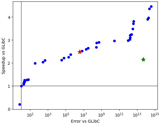
(a) Speed-accuracy Pareto curve for Equation 5

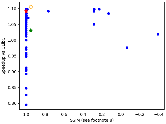
(b) Speed-accuracy Pareto curve for POV-Ray

Figure 3. Speed vs. accuracy for various configurations of Equation 5. On the left, speed and accuracy for just Equation 5; on the right, speed and accuracy for POV-Ray as a whole (on the grenadine scene). Speedup is normalized to the all-GLibC configuration. OpTuner’s configurations are marked in blue and red, while the POV-Ray developers’ custom implementation is marked with a green star. OpTuner’s tuned configurations are both faster and more accurate than the developers’ custom implementation. The orange circle in the graph on the right relates to future work described in Appendix A.

Using OpTuner’s suggested configurations can lead to end-to-end application speedups. We produced modified versions of POV-Ray for each of OpTuner’s suggested configurations and plotted both their overall run time and the quality of their outputs in Figure 3(b). POV-Ray is a naturally-error-tolerant program as shown by the blue streak on the left-hand-side of the figure: OpTuner’s $78$ most accurate configurations all render the reference image exactly. Likewise, there’s a limit to how much POV-Ray can be sped up just by changing function implementation, for Amdahl’s-law-like reasons. The red starred configuration hits both these limits, with results identical to the reference rendering, but produced roughly $9\%$ faster. By contrast, the green starred point, which is the POV-Ray developers’ implementation, is both slower and has noticable errors (Figure 2). Of course, it is up to the POV-Ray developers to decide how much accuracy loss is acceptable and how large a speed-up makes up for a given level of error. But here, OpTuner’s proposed configurations are simultaneously faster and more accurate. Moreover, the point marked in red is not the only option produced by OpTuner; the developers can experiment with different configurations and easily find one that is faster and less accurate if they so desire.

4. Mathematical Function Implementation Background

While the mathematics behind approximating transcendental functions is well understood, numerous choices, like approximation method, polynomial order, table size, and range reduction strategy, all impact both accuracy and speed.

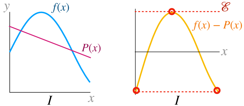
(a) Polynomial approximation and error

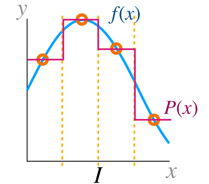
(b) Table approximation

Figure 4. Approximations $P(x)$ of an arbitrary function $f(x)$. A order-1 polynomial approximation is shown on the left; a $4$-entry table based approximation is shown on the right. In the middle, an illustration of the equioscillation theorem: the polynomial approximation is optimal error reaches its highest value the maximum number of times.

double ml2_raw_wide_sin_13(double x){
  double x2 = x * x;
  double pa, pa1, pa3, pa5, pa7, pa9, pa11, pa13;
  pa13 =  0x1.52a851954275cp-33;
  pa11 = -0x1.ae00bdd2a86a8p-26 + x2 * pa13;
  pa9  =  0x1.71dce463cf737p-19 + x2 * pa11;
  pa7  = -0x1.a019fce360596p-13 + x2 * pa9;
  pa5  =  0x1.11111109020a6p-7  + x2 * pa7;
  pa3  = -0x1.5555555540916p-3  + x2 * pa5;
  pa1  =  0x1.ffffffffffdc9p-1  + x2 * pa3;
  pa   = x * pa1;
  return pa;
}

(a) An order-13 polynomial function approximation

double sin_table[255];

void fill_table() {
  for(i=0; i<255; i++){
    theta = (double)(i-127)*M_PI/127.0;
    sin_table[i] = sin(theta);
  }
}

double table_sin(double x){
  int index = (x*127.0/M_PI) + 127;
  return sin_table[index];
}

(b) A size-255 table-based function approximation

Figure 5. Two possible approximations of sin for $x\in[-\pi,\pi]$. The one on the left uses an order-13 order polynomial and achieves an absolute error of $3.87\cdot 10^{-6}$ and a run time of $3.85$ nanoseconds on our reference machine. The on on the right is the table based implementation used by POV-Ray, with an absolute error of $0.02473$ and a run time of $3.19$ nanoseconds.

4.1. Approximating over an Interval

The core technique in implementing a mathematical function is approximating a function $f$ over a small input range $I$. One method is to find a polynomial $P(x)$ that approximates $f$. While techniques like Taylor series and Chebyshev approximations, which optimize for the average case, are better known, implementations usually optimize for worst-case errors. The Remez exchange algorithm (Pachón and Trefethen, 2009), which solves for local minima and maxima of $f(x)-P(x)$ by the Chebyshev equioscillation theorem (Mayans, 2006), is the standard way of deriving coefficients for $P$ that minimize worst-case error. Figure 4(a) illustrates this approach. Remez exchange is implemented in the the Sollya tool (S. Chevillard et al., 2010), which additionally uses the LLL algorithm (Lenstra et al., 1982) to tune the coefficients for the floating-point domain. The end result of this process is an implementation similar to the one shown in Figure 5(a). The number of terms in the polynomial is the key parameter to this process; an implementation can approximate a target functions like $\sin$ or $\exp$ with anywhere from one to dozens of terms, offering a spectrum with higher-order approximations being more accurate but also slower. The input interval $I$ is also an important input; generally speaking, wider input intervals yield worse approximations. Even once a polynomial is found, there are more choices to make. For example, the polynomial $P(x)=a_{0}+a_{1}\cdot x+a_{2}\cdot x^{2}+\dotsb$ is usually evaluated via Horner’s rule, $P(x)=a_{0}+x\cdot(a_{1}+x\cdot(a_{2}+x\cdot(\dotsb)))$, but there are other evaluation schemes as well, like Estrin’s Method for parallelization with SIMD or compensated summation for higher accuracy.

Table-based implementations are an alternative to pure polynomial approximation. In a table-based implementation, the interval $I$ is split into many smaller intervals, often hundreds or thousands of them, and then some uniform method is used to approximate the function on each of those smaller intervals. A simple table-based implementation like this tabulates $f(x)$ for evenly spaced $x$ values, like the $\sin$ table in the back of an old-school math textbook; such an implementation is shown in Figure 5(b). A more sophisticated approach may store polynomial coefficients in the table, or use complex interpolation schemes to fill in intermediate values. Just as with polynomial implementations, a table-based scheme has many parameters for the implementor to choose: table size, interpolation scheme, subdivision algorithm, and so on; and again, these parameters affect both speed and accuracy, and may depend on machine-specific parameters like cache size.

4.2. Range Reduction

Neither polynomial nor table-based approximation works well over a large input interval $I$, so the most challenging part of approximating a mathematical function is making sure the function can be applied to an arbitrary input. This is called range reduction and reconstruction. Range reduction and reconstruction bookend the polynomial or table, transforming the input to lie within the polynomial or table’s input range and then adjusting the output to fit the original input.

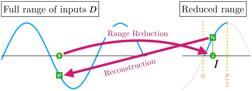
Figure 6. Range reduction and reconstruction for sin. The input point, somewhere along the input domain, is mapped via range reduction into the interval $[0,\pi/2]$ for evaluation, then mapped back via reconstruction to the correct output value. This reduction takes advantage of the cyclic nature of sin, the symmetry of the sections of sin above and below $y=0$, and the mirror symmetry present in each half cycle. Reconstruction of sin needs only determine the correct sign of the output.

Consider implementing sin over a large range. Since sin is periodic, $\sin(x)=\sin(x\bmod 2\pi)$; and furthermore, $x\bmod 2\pi$ is bounded to the range $[0,2\pi]$. Thus, sin can be implemented over a large range by using a polynomial or table for the range $[0,2\pi]$ and reducing other inputs to lie within that range. We can take advantage of other symmetries to restrict the range further. For example, $\sin(x)=-\sin(x-\pi)$; for inputs $x\in[\pi,2\pi]$ the right hand side of this equation calls $\sin$ on inputs $x-\pi\in[0,\pi]$. So, a polynomial or table fit to $[0,\pi]$ is enough, but in this case a reconstruction step is necessary to take the output on the reduced input (in this case, $\sin(x-\pi)$) and compute from it the output for the original input (in this case, by negating the reduced output). Both reduction and reconstruction are shown in fig. 6. Other identities, like the double-angle formula, can also be used for range reduction, and the same general principle of using function identities to reduce the input range can apply to $\log$, $\exp$, or any other functions with identities to leverage.

Reducing the interval $I$ that the polynomial or table is fit to usually makes the approximation itself either more accurate or faster (by using fewer terms). But range reduction and reconstruction can slow the implementation down and add error of their own. Traditionally, math libraries have used higher-precision arithmetic, such as in Cody & Waite reduction (Cody, 1980), to implement range reduction with no error. This maximizes accuracy, especially for very large inputs (imagine computing $\text{{sin}}(10^{10})$), but is also very slow because it requires computing $x\bmod 2\pi$ in very high precision using thousands of bits of $\pi$. But range reduction can also trade accuracy for speed. For example, $x\bmod 2\pi$ can be computed by just evaluating $x-\lfloor x/2\pi\rfloor$ in double precision. This introduces errors (from approximating $\pi$ and from division) but is significantly faster than high-precision arithmetic. There are also intermediate choices with more or less error. Thus, the choice of range reduction again presents a trade-off between accuracy and speed.

5. Error and cost models

The input to OpTuner is a floating-point expression $\tilde{E}$, with no loops or control flow, over some number of floating-point inputs; for simplicity, this section refers to a single input $x_{0}$, though generalizing to multiple inputs is straightforward. In addition to the expression $\tilde{E}$, the input must also contain an interval $I$ that the input $x_{0}$ is drawn from. The core idea behind OpTuner, as described in Section 2, is the linear error model for a floating-point expression. To compute the error model OpTuner uses error Taylor series (Solovyev et al., 2018).

5.1. Error model

Take a floating-point expression $\tilde{E}$ generated by the grammar $e::=\tilde{f}(e,e,\ldots)\mid x_{0}$. In this paper, variables with tildes, like $\tilde{x}_{i}$, represent floating-point values, and the same variables without tildes, like $x_{i}$, represent their true mathematical value when computed without rounding error. Each $\tilde{f}$ thus implements of some underlying function $f$; floating-point constants like PI can be considered zero-argument functions.

Transform the expression $\tilde{E}$ to a linear sequence of function calls $\tilde{x}_{n}:=\tilde{f_{n}}(\tilde{x}_{n-a_{n}},\tilde{x}_{n-b_{n}},\ldots)$, where later function calls may use the results of earlier calls as arguments, and where the value of the expression as a whole is the value of the last variable in the sequence, $\tilde{x}_{N}$. By eq. 1, $\tilde{x}_{n}=f_{n}(\tilde{x}_{n-a_{n}},\tilde{x}_{n-b_{n}},\ldots)(1+\varepsilon_{n})+\delta_{n}$. Note that $\tilde{x}_{N}$ is thus a function of the $\varepsilon_{n}$s and $\delta_{n}$s. When all $\varepsilon_{n}=\delta_{n}=0$, the result is $x_{n}$ computed without any error; but $\varepsilon_{n}$ and $\delta_{n}$ are not equal to zero. Instead they are small, unkown values bounded by constants $\varepsilon_{f_{n}}$ and $\delta_{f_{n}}$.

Define the constants

$$A^{k}_{n}=\max_{x\in I}\left(\frac{\partial\tilde{x}_{k}}{\partial\varepsilon_{n}}\left[\begin{array}[]{l}0/\varepsilon\\ 0/\delta\end{array}\right]\right)\;\text{and}\;B^{k}_{n}=\max_{x\in I}\left(\frac{\partial\tilde{x}_{k}}{\partial\delta_{n}}\left[\begin{array}[]{l}0/\varepsilon\\ 0/\delta\end{array}\right]\right)$$

and $A_{n}=A^{N}_{n}$ and $B_{n}=B^{N}_{n}$. Note that these constants are real numbers and can be computed by a one-dimensional global nonlinear optimization; or, for expressions with multiple variables, over as many dimensions as there are input variables. Then the error of $\tilde{E}$ is:

(7) $$|\tilde{x}_{N}-x_{N}|\leq\sum_{n}A_{n}\varepsilon_{f_{n}}+\sum_{n}B_{n}\delta_{f_{n}}+o(\varepsilon^{2}).$$

Here, the $o(\varepsilon^{2})$ term represents the quadratic and higher-order terms of the error Taylor series. It can be bounded using Lagrange’s theorem,

$$o(\varepsilon^{2})\leq\max_{x\in I}\left(\sum_{u,v\in\{\varepsilon,\delta\}}\sum_{i,j}\frac{\partial^{2}x_{k}}{\partial u_{i}\partial v_{i}}\left[\begin{array}[]{l}0/\varepsilon\\ 0/\delta\end{array}\right]u_{f_{i}}v_{f_{j}}\right),$$

where the sums range over all pairs of $\varepsilon/\delta$ variables. Importantly, since this bound involves higher powers of the $\varepsilon_{f}$s and $\delta_{f}$s, it tends to be insignificantly small. It is necessary for soundness, but is not particularly important for estimating the error.

Equation 7, including the Lagrange bound for the higher-order terms, is the traditional use of error Taylor series. OpTuner instead drops the higher-order terms and considers the remaining linear terms as a function of the $\varepsilon$ and $\delta$ variables that estimates $\tilde{E}$’s error in terms of the function implementations it uses. Note that typically, an expression contains operators like addition and multiplication that OpTuner cannot tune. In this case some of the $\varepsilon$ and $\delta$s are fixed and OpTuner folds those resulting terms into a constant.

5.2. Cost model

The complement to the linear error model is a linear cost model, which estimates the speed of the expression given the implementations chosen for each function call. OpTuner uses a simple cost model:

$$\mathit{cost}=\sum_{n}c_{f_{n}},$$

where $c_{f}$ is the average runtime of the function implementation $\tilde{f}$. To measure $c_{f}$, each implementation is compiled and run on $163840$ random valid inputs in a tight loop for $10$ seconds. To try to get maximally accurate timings. we use multiple measurements, input pre-generation, core binding, and the -O3 -march=native -mtune=native -DNDEBUG compiler flags.

Normally, a simple sum of average runtimes is too simplistic: it ignores the complexities of modern CPUs and the details of input-dependent control flow. Several factors make this model more appropriate in our setting. OpTuner’s goal is to find all Pareto-optimal trade-offs between the error and cost models, so the cost model only needs to be a relative order, not a precise prediction of runtimes. Plus, mathematical function implementations usually have rare, easily-branch-predicted control flow; use few if any data structures or complex memory access patterns; and are generally compute-bound. That makes average runtimes more meaningful than for general-purpose code. Finally, since OpTuner only changes the implementation of mathematical functions, any computation outside a function implementation will be the same across all configurations. The cost model thus does not need to model those costs, and is only predicting the costs of calls to shared libraries.

One caveat is necessary for achieving good results with this cost model: the linear sequence of function calls $x_{n}=\tilde{f}_{n}(x_{n-a_{n}},x_{n-b_{n}},\ldots)$ must contain no duplicate entries representing common subexpressions. Compilers commonly perform common subexpression elimination to avoid recomputing the same expression twice. Thus, if two subexpressions both compute $f(x_{1},x_{2})$, and the first subexpression uses implementation $\tilde{f}_{a}$ while the second uses implementation $\tilde{f}_{b}$, the cost is $c_{a}+c_{b}$ if these implementations are different but only $c_{a}$ is both implementations are the more accurate of the two. In other words, when common subexpressions exist, it’s best to use the same, more accurate implementation at both sites. OpTuner thus performs common subexpression elimination when converting expressions to a linear sequence of function calls, and the cost and error models are built on this deduplicated sequence, ensuring that common subexpressions use the same implementations.

5.3. Mathematical Libraries

Func	Domain	Error	Cost	Library
exp	$[-1.79e^{308},$ $709.78]$	0.5	54.02	CRLibM
		1.0	10.71	GLibC
			10.70	OpenLibm
			10.78	AMD LibM
		5.0	5.32	VDT
log	$[5.0e^{-324},$ $1.79e^{30}]$	0.5	32.93	CRLibM
		1.0	8.53	GLibC
			8.53	OpenLibm
			8.36	AMD LibM
		5.0	5.99	VDT
sin	$[-1.79e^{308},$ $1.79e^{308}]$	0.5	35.27	CRLibM
		1.0	8.76	GLibC
			8.76	OpenLibm
			7.56	AMD LibM
		5.0	4.42	VDT
	$[-0.78,0.78]$	5.0	1.82	VDT
cos	$[-1.79e^{308},$ $1.79e^{308}]$	0.5	34.35	CRLibM
		1.0	8.84	GLibC
			8.82	OpenLibm
			7.19	AMD LibM
		5.0	4.20	VDT
	$[-0.78,0.78]$	5.0	2.04	VDT
tan	$[-1.79e^{308},$ $1.79e^{308}]$	0.5	80.20	CRLibM
		1.0	15.81	GLibC
			16.00	OpenLibm
			28.66	AMD LibM
		5.0	8.90	VDT

(a) Double precision implementations

Func	Domain	Error	Cost	Library
expf	$[-3.40e^{38},$ $88.72]$	$2.68\cdot 10^{8}$	5.06	RLibM
		$4.03\cdot 10^{8}$	8.46	GLibC
			4.86	OpenLibm
			4.68	AMD LibM
		$1.76\cdot 10^{10}$	5.20	VDT
logf	$[1.40e^{-45},$ $3.40e^{38}]$	$2.68\cdot 10^{8}$	6.26	RLibM
		$2.76\cdot 10^{8}$	7.15	GLibC
			7.13	OpenLibm
			5.88	AMD LibM
		$5.45\cdot 10^{8}$	5.80	VDT
sinf	$[-3.40e^{38},$ $3.40e^{38}]$	$2.16\cdot 10^{9}$	7.13	GLibC
			7.10	OpenLibm
			7.64	AMD LibM
		$1.74\cdot 10^{10}$	4.69	VDT
	$[-0.785,0.785]$	$1.74\cdot 10^{10}$	1.60	VDT
cosf	$[-3.40e^{38},$ $3.40e^{38}]$	$2.16\cdot 10^{9}$	7.13	GLibC
			7.10	OpenLibm
			6.76	AMD LibM
		$1.74\cdot 10^{10}$	4.47	VDT
	$[-0.785,0.785]$	$1.74\cdot 10^{10}$	1.93	VDT
tanf	$[-3.40e^{38},$ $3.40e^{38}]$	$5.37\cdot 10^{8}$	8.50	GLibC
			8.49	OpenLibm
			7.03	AMD Libm
		$1.77\cdot 10^{10}$	8.32	VDT

(b) Single precision implementations

Figure 7. The standard library implementations available to OpTuner. Errors were found via documentation and source code comments and are given in “units in the last place”; the actual $\varepsilon_{f}$ and $\delta_{f}$ values are the listed error times $2^{-52}$ for $\varepsilon_{f}$ and $2^{-1022}$ for $\delta_{f}$. There is a general trade-off between speed and accuracy, though with a lot of heterogeneity between libraries and functions.

Implementations of mathematical functions are usually gathered into libraries that provide a large collection of functions all at a similar point in the speed-accuracy trade-off. These libraries broadly cover a spectrum from faster, less-accurate implementations to slower, more-accurate ones. OpTuner ships with support for many of the most popular libraries, covering a range of accuracies and speeds; Figure 7 lists these libraries and their error and cost model parameters $D$, $\varepsilon_{f}$, $\delta_{f}$, and $c_{f}$.

The golden standard for function implementation are correctly rounded implementations. These yield the true mathematical result, rounded to floating-point; this value is unique, so all correctly-rounded libraries produce identical answers on all inputs. Unfortunately, achieving this accuracy is still a topic of active research. CRLibM provides correctly-rounded implementations of many math functions in double precision, but it is quite slower, usually by a factor of $5$–$10\times$, than a traditional implementation. Work on reducing this overhead is ongoing. The recently-published RLibM library achieves correct rounding and speed comparable to alternative libraries using techniques from program synthesis and verification. However, its techniques do not scale to 64-bit implementations, so RLibM only provides 32-bit implementations and furthermore only for a small set of mathematical functions not including, for example, sin and cos. Ultimately, neither CRLibM or Rlibm is (currently) in common use, showing that most users have already decided on higher speed in exchange for lower accuracy.

Standard system math libraries aim for nearly-correct rounding. These libraries, which include GLibC, OpenLibm, and AMD Libm, aim to achieve the highest possible performance while allowing the least- or even second-least-significant bit to be incorrect. Being marginally less accurate than CRLibM and RLibM often allows them to be dramatically faster. Consequently, these libraries are appropriate for general-purpose code, where speed is a top-level concern but where programmers do not have the expertise to optimize the speed-accuracy trade-off further. Different libraries in this category use different implementation strategies in order to achieve maximum speed, including (often) custom implementations for specific hardware architectures or generations. For example, GLibC has roughly a dozen architecture-specific implementations of the main mathematical functions.

In some domains, greater speed and lower accuracy are required; for such programs, special-purpose mathematical libraries exist. For example, the VDT library, developed by CERN, allows for up to 3 incorrect bits, two more than the standard system library (more in single precision). In exchange for lower accuracy, VDT can be up to twice as fast as the corresponding GLibC function and also has some vectorization advantages. VDT uses Padé approximations (a variant on polynomial approximations) and tunes them to slightly lower accuracy in order to achieve this speedup.

Finally, some applications are best run at a speed-accuracy trade-off not represented by any of the above libraries. For such cases, MetaLibm provides a metaprogramming framework ideal for generating new function implementations. MetaLibm provides easy access to polynomial generation with Sollya, a convenient cross-compilation mechanism, and utility routines useful for writing function implementations. Of particular interest is that MetaLibm implementations can be parameterized; for example, MetaLibm’s exp implementation can be parameterized by any number of polynomial terms. Besides the specific implementations that ship with MetaLibm, such as the parameterized exp implementation, users can also use MetaLibm to write their own custom implementations.

Some libraries also provide multiple implementations of the same function for tuning purposes. The simplest case of this is providing different implementations for single- and double-precision arguments: single-precision versions are fundamentally less accurate due to rounding, so different parameter choices are advised. The single-precision versions also usually have a narrow input range. Usually the single-precision version is not implemented independently; instead it uses a truncated and rounded form of the polynomial used for the double function. (This is not optimal, but economizes on the high cost of developing a novel function implementation.) Some libraries also provide function implementations valid over only a certain input range, which allows those implementations to skip (or simplify) range reduction. For example, the VDT library internally contains implementations of sin and cos which are valid only on the reduced range $[-\pi/2,\pi/2]$. These types of implementations are intended to be used with external range reduction, and are often not exposed at a library level, but using them directly can lead to generous advantages in speed. The bar to using these implementations is proving that the input will be in the reduced range.

6. Selecting optimal implementations

Between the various libraries listed above, and the parameterized implementations from MetaLibm, there are dozens of implementations of sin, cos, tan, exp, and log, which makes selecting the right one a chore. OpTuner uses its error and cost models to encode the implementation selection problem as an integer linear program and select the right configurations automatically.

6.1. Encoding Configuration Selection

DefVar  t_i,j ∈{ 0, 1 } PickOne  ∑_j t_i, j = 1 SetEps  ε_i = ∑_j t_i,j ε_f_j ∧δ_i = ∑_j t_i,j δ_f_j MinErr  min∑_i A_i ε_i + ∑_i B_i δ_i SetCost  c_i = ∑_j t_i,j c_f_j MinCost  min∑_i c_i

Figure 8. And integer-linear-program formulation of the implementation selection problem.

A valid implementation selection must minimize both overall error and execution time while making a discrete choice of implementation for each use site. This naturally fits the integer linear programming paradigm; a full integer linear program is given in Figure 8. The key decision variables for the linear program are boolean variables that determine which implementation is used at each use site: $n\times m$ boolean variables $t_{i,j}$, where $t_{i,j}$ is true if use site $i$ uses implementation $f_{j}$ (DefVar). Note that for a fixed $i$, the $t_{i,j}$ sum to 1 (PickOne).

The two key constraints on these decision variables are to minimize the error and cost models. First, the $\varepsilon_{i}$, $\delta_{i}$, and cost $c_{i}$ of the chosen implementation for each use site $i$ are computed (SetEps and SetCost). Note that these constraints embed the $\varepsilon_{f}$, $\delta_{f}$, and $c_{f}$ constants for the available implementations of each function. Then, the error and cost models are minimized in the integer linear program. The cost model is just the sum of per-use-site costs, so is simple to express (MinCost). The error model, on the other hand, is the linear expression described in Section 5. In our implementation error Taylor series are computed with FPTaylor (Solovyev et al., 2018) and each optimization problem is solved using the Gelpia (Baranowski et al., 2018) sound global nonlinear optimization engine.

To solve these constraints, the integer-linear-program solver must support two additional features. The $\varepsilon_{f_{j}}$ and $\delta_{f_{j}}$ coefficients in this linear program typically vary dramatically in magnitude, (rounding error can differ dramatically between implementations). Unfortunately, many common ILP solvers produce errors or invalid solutions when coefficients vary so widely, likely due to rounding error inside the solver itself. An exact rational ILP solver is thus necessary. Furthermore, the error and cost models are usually at odds with one another and cannot be minimized simultaneously. Instead of a single solution to the conflicting goals there is a set of points where decreasing error must increase cost, and vice versa. The ILP solver in question must implement a Pareto mode which can find this set automatically. (Repeated ILP queries with a varying error bound also work, but an in-solver Pareto mode is typically much more efficient.) OpTuner uses Z3 as its ILP solver (de Moura and Bjørner, 2008); Z3 uses exact rational arithmetic and has an efficient Pareto mode. A particularly handy aspect of Z3’s Pareto modes is that the points are generated sequentially, not all at once, so users can start exploring OpTuner-suggested configurations even while OpTuner is still running.

6.2. Verification and Timing

The Pareto-optimal solutions to the integer linear program in Figure 8 are Pareto-optimal for OpTuner’s error and cost models. But modeled and real speed and accuracy, differ enough to shift the position of the points. OpTuner thus recomputes true error and measures actual speed in a post pass.

OpTuner’s error model simplifies floating-point error in several ways. For one, eq. 1 mildly overestimates floating point error. Dropping higher-order terms from the error Taylor form then underestimates error when the $\varepsilon$ and $\delta$ values are large—that is, for particularly inaccurate function implementations. Then, linearizing the error model in eq. 4 overapproximates by ignoring correlations between different terms. So, OpTuner recalculates the accuracy of all configurations returned by the ILP solver using FPTaylor’s most accurate fp-power2 mode. Since the recalculation is working with a fixed implementation selection, the higher-order and correlation terms can be included and a sound worst-case error bound can be returned.

OpTuner’s cost model also oversimplifies. Needless to say, modern CPUs are complex, with features like out-of-order execution and branch prediction that OpTuner’s cost model ignores. Runtime also typically depends on the larger application context; a table-based function implementation runs much faster if the table stays resident in cache. OpTuner thus measures the speed of each configuration returned by the ILP solver. To make sure the measurement is accurate, OpTuner uses the maximum-speed compiler flags, averages multiple measurements, pre-generates random valid inputs, and binds the timing program to a core, just like when computing $c_{f}$ for each implementation.

After accuracies are recalculated and speeds measured, it is possible for some configurations returned by the ILP solver to no longer be on the Pareto frontier—that is, for one of the returned points to in fact be both faster and more accurate than another. OpTuner filters out such points by sorting returned points by actual speed, and removing any points whose accuracy is not monotonically increasing. This filtering is just a convenience for the user, and removes, on average, only $26\%$ of the points. Usually, the points removed by this process are still quite close to the Pareto frontier; however, removing these points means the user needs to explore fewer configurations and can find a good configuration more quickly.

7. Leveraging Restricted Input Ranges

As discussed in Section 5.3, there are advantages to reduced range function implementations: by skipping range reduction entirely, or by using faster but less accurate range reductions, a function implementation can be dramatically sped up without meaningfully increasing its error. However, restricted-range implementations can only be safely used by proving that its input lies within that restricted range.

7.1. Modeling Input Ranges

When a function is called in a floating-point expression, the range of inputs it is called on depends on not only the mathematical value of the input expression but also on how much error that input is computed with. This dependence means that choosing a rougher approximation for one part of a computation can change what implementations are available in a later part of the computation. Determining where a reduced-range implementation can be used is therefore like flattening a rug with a bump in it—as soon as one part is fixed another part pushes back up—because replacing one function implementation with another will also change the range of its output and thus the valid implementations of other function calls. Yet the advantages of reduced-range implementations are too large to pass up.

Formally, consider a sequence of function assignments $\tilde{x}_{n}:=\tilde{f_{n}}(\tilde{x}_{n-a_{n}},\tilde{x}_{n-b_{n}},\ldots)$, except that the function $\tilde{f}_{n}$ is only valid when its first argument is in the range $[d_{1},d_{2}]$ (functions with range restrictions on other arguments work analogously). Since $\tilde{f_{n}}$ is in fact called on $\tilde{x}_{n-a_{n}}$, we must establish that $d_{1}<\tilde{x}_{n-a_{n}}<d_{2}$. Following the idea of the error Taylor series,

$$|\tilde{x}_{n-a_{n}}-x_{n-a_{n}}|\leq\sum_{i}A^{n}_{i}\varepsilon_{f_{i}}+\sum_{i}B^{n}_{i}\delta_{f_{i}}+o(\varepsilon^{2})$$

where the $A^{n}_{i}$ and $B^{n}_{i}$ constants are as defined in Section 5. For now, ignore the higher-order terms. Now, suppose $x_{n-a_{n}}$, the true mathematical value of $\tilde{x}_{n-a_{n}}$, is bounded within $[a_{1},a_{2}]$ for all $x\in I$; OpTuner computes these bounds using Gelpia. The requirement $d_{1}<\tilde{x}_{n-a_{n}}<d_{2}$ can then be rewritten:

$$d_{1}<x_{n-a_{n}}\pm\left(\sum_{i}A^{n}_{i}\varepsilon_{f_{i}}+\sum_{i}B^{n}_{i}\delta_{f_{i}}\right)<d_{2}$$

$$\operatorname{\Longleftrightarrow}\; d_{1}<a_{1}-\left(\sum_{i}A^{n}_{i}\varepsilon_{f_{i}}+\sum_{i}B^{n}_{i}\delta_{f_{i}}\right)\land a_{2}+\left(\sum_{i}A^{n}_{i}\varepsilon_{f_{i}}+\sum_{i}B^{n}_{i}\delta_{f_{i}}\right)<d_{2}$$

$$\operatorname{\Longleftrightarrow}\; \left(\sum_{i}A^{n}_{i}\varepsilon_{f_{i}}+\sum_{i}B^{n}_{i}\delta_{f_{i}}\right)<a_{1}-d_{1}\land\left(\sum_{i}A^{n}_{i}\varepsilon_{f_{i}}+\sum_{i}B^{n}_{i}\delta_{f_{i}}\right)<d_{2}-a_{2}$$

(8) $$\operatorname{\Longleftrightarrow}\; \left(\sum_{i}A^{n}_{i}\varepsilon_{f_{i}}+\sum_{i}B^{n}_{i}\delta_{f_{i}}\right)<\min(a_{1}-d_{1},d_{2}-a_{2})$$

Define the constant $S_{i,j}$ to be the right hand side value, $\min(a_{1}-d_{1},d_{2}-a_{2})$, for using implementation $\tilde{f}_{j}$ at use site $i$. Crucially, the right hand side value depends only on the function input range $[d_{1},d_{2}]$ and the argument’s error-free range $[a_{1},a_{2}]$. Thus, the final inequality of Equation 8 is a linear inequality over the same $\varepsilon$ and $\delta$ variables as the integer linear program in Section 6. OpTuner adds the following inequality to the integer linear program:

$$\framebox{{InRange}}\;t_{i,j}\implies\sum_{k}A^{i}_{k}\varepsilon_{k}+\sum_{k}B^{i}_{k}\delta_{k}<S_{i,j},$$

The implication can also be written as a pure ILP statement, but the ILP solver OpTuner uses, Z3, supports implication statements like these directly. Note that in some cases, the constant $S_{i,j}$ can be negative, meaning that $\tilde{f}_{j}$ cannot be used.

Just like with OpTuner’s use of the linear error model, a post-pass is necessary to take into account the higher-order terms that OpTuner ignores during ILP solving. This post-pass recomputes the input range using the most accurate rounding model and with higher-order terms bounded using Lagrange’s theorem, and removes the point from the speed-accuracy Pareto curve if adding the higher-order terms makes the chosen implementations invalid. In practice this occurs for $11.0\%$ of points, mostly at the far end of the Pareto curve where error is already high.

7.2. Implementing New Restricted-range Libraries

To test OpTuner’s support for restricted input ranges, we used MetaLibm to implement custom restricted-range versions of $\sin$, $\cos$, $\tan$, $\exp$, and $\log$. Our implementations are based on those of Green (2002, 2020): they fit a polynomial of 1–$16$ terms using over a function-specific core interval $I$, and then use either no range reduction or a custom, simplified range reduction without higher-precision arithmetic operations. Since these range reductions use simplified arithmetic, they are accurate over roughly 1–50 multiples of $I$, with an accuracy/input range trade-off on top of the accuracy/speed trade-off. Traditionally, restricted-range implementations are hidden from library users because it is too easy to misuse them. Because OpTuner is sound, this fear no longer applies.

Implementing these functions was relatively straightforward thanks to MetaLibm, but deriving accuracy bounds was more challenging. Inaccuracy—error—comes from three sources: algorithmic error, or the difference between the polynomial and the function being implemented; rounding error, or the error of evaluating the polynomial in floating-point arithmetic; and reduction error from error in the range reduction and reconstruction steps. To derive a sound bound we bound each type of error separately and then sum them, once for the $\varepsilon$ parameter and once for the $\delta$ parameter. The algorithmic error is a purely mathematical artifact, and Sollya can compute it automatically (it is computed in the inner loop of the Remez exchange algorithm). To bound the rounding error we use FPTaylor with the most accurate fp-power2 error model. While FPTaylor’s bounds are very tight they can in rare cases be edged out by manual error analysis, such as Oliver (1979)’s bound on the rounding error of a Horner-form polynomial. To get the best possible bound we use the tigher of FPTaylor’s and Oliver’s bound, since both are sound error estimates. The reduction error, however, is harder to analyze.

Range reduction typically involves a mix of integer and floating-point computations, so to bound it we use the approach of Lee, Sharma, and Aiken (Lee et al., 2016). In mixed integer-floating point computations the integer values are constant for some range of floating-point values; for example, when rounding a floating-point value to an integer; all of the float values in the range $[0.5,1.5]$ round to $1$. A single mixed-integer-floating-point computation is therefore broken down into multiple computations only floating-point variables and integer constants, where different computations are used for different $x$ values. Our restricted-range implementations compute $k=\lfloor x/\pi\rfloor$; this expression for $k$ is monotonic so a fixed $k$ values corresponds to an interval of $x$ values. The error of the remaining floating-point operations is computed using FPTaylor, and FPTaylor is again used to determine how the approximating polynomial modulates that error. Aggregating across all $k$ values results in the overall reduction error. Generally, larger $k$ values lead to larger input ranges but also greater error. To account for this, we give a single implementation multiple accuracy specifications (as if it were multiple functions) with narrower input ranges having lower error.

On the 8-core machine used for this paper, verifying the bounds for the complete collection of $216$ custom implementations of exp, log, sin, cos, and tan takes approximately $2$ hours. On average, for each implementation, generating the approximating polynomial takes $5$ minutes, verifying its accuracy without range reduction takes $3$ minutes, and verifying its accuracy with range reduction takes an additional $3$ minutes for each $k$ bound. Importantly, though verifying these implementations takes a lot of time, it only needs to be done once, and the resulting implementations and accuracy bounds are distributed with OpTuner.

8. Evaluation

We evaluate whether OpTuner can automatically select function implementations to achieve a trade-off between speed and accuracy. The data is gathered on a machine with an Intel i7-4793K processor and 32GB of DDR3 memory running Debian 10.10 (Buster), GCC 8.3.0, GLibC 2.28, Sollya 7.0, and Python 3.7.3.

8.1. Methodology

Function $\sin(x)$	Function $\cos(x)$	Function $\tan(x)$
$\bullet$: $D=[-62.83,64.40]$	$\bullet$: $D=[-62.83,64.40]$	$\bullet$: $D=[-39.26,40.05]$
$\bullet$: $D=[-1.571,1.571]$	$\bullet$: $D=[-1.571,1.571]$	$\bullet$: $D=[-0.1,0.89]$
$\bullet$: $D=[-3.142,3.142]$	$\bullet$: $D=[-3.142,3.142]$

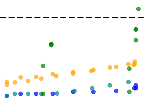
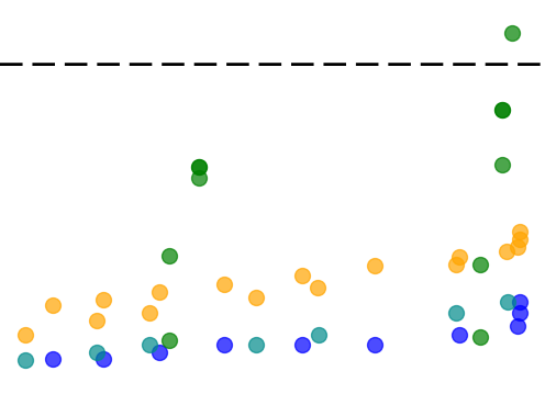
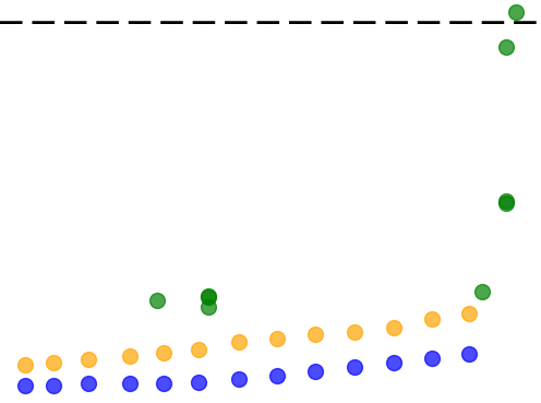
Legend
$\bullet$: Standard libraries
$\bullet$: MetaLibm exp
Custom:
$\bullet$: mild range reduction
$\bullet$: no range reduction
$\bullet$: no range reduction

Function $\exp(x)$	Function $\log(x)$
$\bullet$: $D=[-34.75,35.45]$	$\bullet$: $D=[1.5\cdot 10^{-4},4096]$
$\bullet$: $D=[-0.1,0.79]$	$\bullet$: $D=[0.65,1.6]$

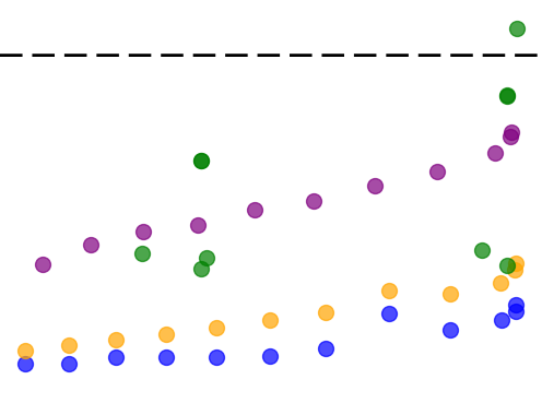
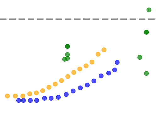
Figure 9. The available implementations for OpTuner. Accuracy is shown in log-scale on the horizontal axis, while runtime is plotted on the vertical axis. The plot’s bottom border represents a runtime of 0, while the dashed line is a break in the vertical axis with CRLibM lying above the break. Note that the synthesized implementations with simplified range reduction are significantly faster.

We evaluate OpTuner on $37$ benchmarks from the FPBench suite (Damouche et al., 2016) as well as the haskell benchmark suite from Herbie 1.5 (Panchekha et al., 2015), originally extracted from Haskell packages via a compiler plugin. Specifically, we select all benchmarks that use the exp, log, sin, cos, or tan functions and do not contain loops or tensors (which OpTuner does not support). Within these benchmarks exp, log, sin, cos, and tan are used a collective $89$ times; the only other library function called is a single use of atan, for which we use the GLibC implementation. Thirteen benchmarks have a single input, ten have two inputs, eleven have three inputs, and the remainder have four or more inputs. Some of the benchmarks come equipped with input ranges defined for them, but, for those that did not, we choose input ranges that avoid domain errors such as division by zero.

OpTuner tunes these benchmarks using a total of $216$ implementations of library functions exp, log, sin, cos, and tan drawn from the standard mathematical libraries and parameterized MetaLibm implementations described in Section 5.3. Figure 9 plots the accuracies and costs for standard mathematical libraries (in green); MetaLibm’s parameterized exp implementation (in purple); and OpTuner’s custom, range-restricted implementations (in blue, cyan, and orange). The various implementations span from half an ulp of error to a relative error of $10\%$, and the fastest implementation is usually about $5\times$ faster than GLibC while the slowest is usually about $5\times$ slower. In between these extremes, there is a smooth trade-off between speed and accuracy.

8.2. Results

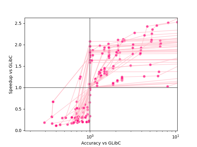
(a) High-accuracy configurations

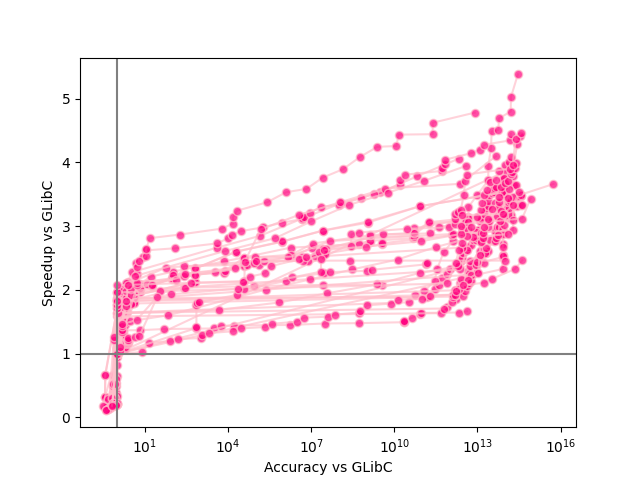
(b) All configurations of any accuracy

Figure 10. OpTuner’s optimized implementations of $37$ benchmarks. Each point’s accuracy and runtime is normalized so that using the GLibC implementations for each function gives a speedup and relative error of $1\times$.

Figure 10 contains all $37$ speed-accuracy Pareto curves, with $1175$ configurations in total. In the plot, each line represents a single benchmark, and each heavy dot along that line is a configuration produced by OpTuner. The benchmarks are normalized so that the “standard” implementation that uses GlibC for each use site is at $(1,1)$.

On the left, in Figure 10(a), are all benchmark implementations with error no more than $10\times$ larger than the standard implementation. Note that even with just one decimal digit more error, speedups of $50\%$, $100\%$ and sometimes even $150\%$ are possible. Note also the cluster of points below and to the left of $(1,1)$. These points represent configurations that are more accurate but also slower than GLibC, generally using the correctly-rounded CRLibM functions. A few points in the plot are above and to the left of $(1,1)$: these configurations are both faster and more accurate than GLibC, generally by mixing CRLibM and custom implementations. In this case, OpTuner is truly offering speed for free. All told, Figure 10(a) shows than OpTuner can produce impressive speedups with minimal expertise or knowledge of numerical analysis.

The right-hand plot, in Figure 10(b), instead focuses on applications tolerant of significant error, such as POV-Ray. Here, implementations with dramatically higher error are plotted, and correspondingly larger speedups are achieved. The points on this figure generally use OpTuner’s custom implementations, which are the fastest ones available. The speedups here are as large as $438\%$. However, the available speedup is limited in benchmarks that use mathematical operations that OpTuner does not tune and in benchmarks with few use sites. For an average benchmark, therefore, the maximum speedup reaches $244\%$. Of course, by the logic of the Pareto curve, this maximum speedup comes with minimal accuracy, and not all applications are as error-tolerant as POV-Ray. Nevertheless, the figure shows that most benchmarks’ Pareto curves feature a steady upward slope, meaning that decreasing accuracy consistently buys increasing speed. Many applications could fruitfully use OpTuner to explore the possibilities that this trade-off offers.

On most benchmarks OpTuner runs in a few minutes. OpTuner’s run time depends on several factors: the number of use sites; the complexity of the expression; the number of input arguments; and in a few cases the input range used. On our test machine, $28$ of the $37$ benchmarks complete in under three minutes and $33$ complete in under ten. The remaining four benchmarks contain the most use sites and thus have the most output configurations to verify and time. OpTuner generates output configurations incrementally, so for these slowest benchmarks, users would have OpTuner’s first configurations available much sooner, usually a few minutes in.

8.3. Detailed Analysis

A close inspection of the OpTuner’s selected configurations demonstrates that these speedups often come from noticing use sites that have little impact on accuracy. Consider the benchmark problem_3_3_2, originally from a mathematical textbook (Hamming, 1986):

$$\begin{array}[]{l}\text{{require}}\>0\leq\mathit{x}\leq 0.75\land 0\leq\mathit{eps}\leq 0.0078125\\ \text{{return}}\>\tan(\mathit{x}+\mathit{eps})-\tan(\mathit{x})\end{array}$$

OpTuner mixes GLibC’s tan for the first call and VDT’s tan for the second to give a $17\%$ speedup over pure GLibC while only increasing relative error from $6.47\cdot 10^{-16}$ to $8.99\cdot 10^{-15}$. The first call to tan has a larger argument than the second call to tan, and due to tan’s steep increase in the region just to the right of $0$ this gives the first call a higher impact on overall accuracy. OpTuner notices this and uses a more accurate implementation for the first call than the second call.

OpTuner’s optimizations can be even more subtle; consider this complex sine benchmark:

$$\begin{array}[]{l}\text{{require}}\>0\leq\mathit{re}\leq 10\land 0\leq\mathit{im}\leq 10\\ \text{{return}}\>(0.5\cdot\sin(\mathit{re}))\cdot(\exp(-\mathit{im})-\exp(\mathit{im}))\end{array}$$

The second call to exp requires more accuracy than the first because $\mathit{im}$ is positive, so the first exp returns smaller values than the second and thus has less impact on the expression’s error. Meanwhile, the output of the sin call is multiplied $\exp(-\mathit{im})+\exp(\mathit{im})$ and its error is thus magnified. In view of these effects, OpTuner selects a high accuracy sin (such as CRLibM’s) and two different exp implementations (say, order-9 and order-12 custom implementations) along the speed-accuracy Pareto curve. This unintuitive mix of implementations leads to a $79\%$ speedup over an all GlibC configuration while only increasing error from $2.25\cdot 10^{-11}$ to $8.65\cdot 10^{-11}$.

These same patterns occur far along the speed-accuracy Pareto curve. Consider the logexp benchmark:

$$\begin{array}[]{l}\text{{require}}\>0\leq x\leq 8\\ \text{{return}}\>\log(1+\exp(x))\end{array}$$

At lower accuracies OpTuner will select VDT’s float variation of log and a custom order-7 exp implementation. This yields a speedup of $205\%$, paid for an accuracy drop from $4.61\cdot 10^{-15}$ to $4.99\cdot 10^{-6}$. As in all these examples, the most important thing to note is the extensive expertise and time commitment necessary to do a similar optimizations by hand.

9. Related Work

Implementing mathematical functions in floating point has a long history. Kahan (1967, 2004), Higham (2002), Muller (2016), and Cody (1980) all made monumental contributions to the field. These authors all leveraged earlier work on approximation theory developed by mathematicians like Pafnutiy Chebyshev and Charles-Jean de la Vallée Poussin. Robin Green’s recent talks on the topic [(2002; 2020)] are a good introduction to and survey of the field. Standard library implementations tend to be accurate to within 1 or a few ulps (FSF, 2020), but some implementations have been produced with a “gold-standard” accuracy of a half ulp, including MPFR (Fousse et al., 2007) and CRLibm (Daramy et al., 2003). Most implementations of library functions like exp or sin are manually verified, and bugs are sometimes discovered (Dawson, 2014; Green, 2002). However, a few of the Intel Math Kernel Library implementations of functions like log, sin, and tan have been verified with semi-automated methods (Lee et al., 2017), and some verified synthesis techniques are available (Lim et al., 2020). OpTuner could these libraries or any other libraries.

Using lower-accuracy library function implementations is an established, if infrequent, program optimization technique. The CERN math library used in OpTuner, VDT (Piparo et al., 2014), was created to allow developers to manually tune this tradeoff. VDT is also carefully optimized for SIMD support, which OpTuner does not currently attempt. There are other similar libraries that OpTuner does not yet incorporate such as Intel MKL (Intel, 2020), CEPHES (Moshier, 1992), and VC’s math functions (VC, 2021).

Darulova and Volkova (2019) have attempted to automate the implementation selection problem in the Daisy numerical compiler (Darulova et al., 2018). In a certain sense, these authors approach a similar problem to OpTuner, but in reverse. In their approach, Daisy starts by analyzing the user’s expression to derive an accuracy bound for each call to a library function. Daisy then leverages MetaLibm’s parametric implementations (Kupriianova and Lauter, 2014) to generate a custom implementation for this accuracy bound. We experimented with using MetaLibm in a similar way. However, we ultimately found that enumerating the space of possible library function implementations was a superior approach, not only because it searches over a broader range of implementation choices than MetaLibm’s parameterized implementations but also because it allows for much more accurate error estimation and thus greater speedups. Daisy also returns a single implementation, while OpTuner returns the full speed-accuracy Pareto curve.

While not specific to floating point, the Green framework (Baek and Chilimbi, 2010) does allow replacing math functions with faster variations in the spirit of approximate computing. Instead of relying on error analysis, the code under test must be accompanied by a quality of service metric. Green provides statistical metrics but does not guarantee worst case behavior. Another downside of this approach is that it scales linearly in the number of possible implementation configurations, which itself grows combinatorially in the number of available implementations and call sites.

Several tools attempt to speeding up floating point computation by computing intermediate values to lower precision. Precimonious (Rubio-González et al., 2013) approaches the problem by sampling points and dynamically testing the speed and error while lowering precision of intermediates in a random search. Blame Analysis (Rubio-González et al., 2016) instead dynamically determines which intermediates have low impact on error, and then select those intermediates as candidates for lowering. HiFPTuner (Guo and Rubio-González, 2018) improves further upon this method by performing a static analysis of the expression to group intermediates and hierarchically search the space of precisions. CRAFT (Lam et al., 2013) is similar to this line of work, but performs the dynamic analysis at a binary level. None of these tools can guarantee a sound error bound. FPTuner (Chiang et al., 2017), on the other hand, performs precision tuning while also guaranteeing an overall error bound. Its use of error Taylor forms and integer linear programming was an inspiration for OpTuner. Optimizing value precision is orthogonal to OpTuner’s purpose, and could potentially integrated into OpTuner.

Other tools improve the accuracy of a floating point expression without an explicit concern for speed. The Herbie (Panchekha et al., 2015) and Salsa (Damouche and Martel, 2018) tools attempt to increase the accuracy of a floating-point expression by rewriting it using algebraic and analytic identities. While these tools do not consider speed, they do sometimes discover rewrites that both increase accuracy and improve runtime (Panchekha et al., 2015). More recently, the Herbie authors have added support for combining rewriting with precision tuning to explore the speed-accuracy trade-off of lower-precision arithmetic (Saiki et al., 2021). Finally, the Stoke tool uses stochastic search over assembly instructions to improve runtime without much reducing accuracy (Schkufza et al., 2014). While this sometimes discovers valuable algebraic rearrangements, this approach cannot implement a complex library function like exp or sin. Stoke also cannot bound the worst-case error of its tuned floating-point expressions; it can only bound the difference between the original and optimized version. In any case, none of these tools currently considers changing the implementation of library functions as OpTuner does. Integrating OpTuner with these tools would likely discover new speedups and further refine the speed-accuracy Pareto curves discovered.

10. Conclusion

OpTuner makes floating-point computations faster by choosing the right implementation of library functions like exp or sin. OpTuner uses a linear error model and integer linear programming to select the best implementations to use (from among standard mathematical libraries and generated implementations) for each use of a library function in a floating-point expression. It then verifies the optimal configurations and presents the user with a speed-accuracy Pareto curve summarizing the available optimization options. Across $37$ benchmarks, OpTuner demonstrates speedups of up to $438\%$, with speedups of $107\%$ available at negligible accuracy increases. OpTuner thus demonstrates the possibilities of a hitherto-underexplored avenue for floating-point program optimization.

Appendix A Appendix: Case Study Methodology

To evaluate POV-Ray’s speed and accuracy for different function implementation configurations, we leveraged the SPEC 2017 benchmark suite, which includes POV-Ray. SPEC 2017 includes a standard compilation harness and a standard quality measure, the structural similarity index measure (Wang et al., 2004), which assigns each $8\times 8$ pixel block a score from $-1$ to $+1$, with $+1$ indicating an exact match. The minimum block score is then used to evaluate image quality, with scores over $0.96$ considered acceptable. The benchmark scene used by SPEC does not use the photons feature, but POV-Ray ships many standard scenes to demonstrate its capabilities, and we use one of those, grenadine, to avoid creating our own contrived example.

The version of POV-Ray included in SPEC 2017 includes and uses the custom sin and cos implementations described in Section 3. These implementations are quite simplistic; a condensed version of sin is shown in Figure 5(b). The input $x$ is converted to an integer from $0$ to $254$ by simple linear transformation: $i=(x/\pi+1)*127$, rounded down. Then a hard-coded table is used to look up $\sin((i-127)*\pi/127)\pi$. This implementation is quite inaccurate—$i$ only has 8 bits of information—but is also quite fast, likely because during a tight loop the hard-coded table stays loaded in cache. OpTuner’s fastest implementations, meanwhile, are all polynomial-based. Nonetheless, some of the configurations it finds are both faster and more accurate than the POV-Ray implementations, suggesting that OpTuner could have helped the POV-Ray developers speed up caustics.

One challenge in this evaluation is the choice of baseline. SPEC uses POV-Ray’s custom table-based implementations to generate its reference image, but as mentioned above those implementations are inaccurate. We therefore modified POV-Ray to use the sin and cos implementations from GLibC, which POV-Ray had historically used (prior to the development of the custom table-based implementations), and used that implementation to generate our reference images as well as our performance baseline. We also verified that a rendering using CRLibM’s (Daramy et al., 2003) sin and cos produces the exact same image; since CRLibM is maximally accurate, this further justifies the use of GLibC as a baseline. Code comments in the POV-Ray source code confirm that before POV-Ray added its custom sin and cos implementations, it used GLibC (or other system math library) implementations, making this baseline historically plausible.

To use OpTuner with POV-Ray, we first extracted the expression seen in Equation 5 and recorded it in FPCore, OpTuner’s input language. The bounds on the input variables were easily established since the angle values were already known to be bounded and the $n$ values come from a unit normal. We then ran OpTuner to generate the configurations along the speed-accuracy Pareto curve. For each resulting configuration, we produced a patched version of POV-Ray by injecting the source code for all of OpTuner’s supported implementations into POV-Ray and using macros and compiler flags to select which one is used. The SPEC harness was then used to determine both the speedup and the quality of the resulting rendering. This allows us to measure OpTuner’s outputs not just in terms of the isolated extracted expression but also in end-to-end real terms for a large and performance-sensitive software project.

Besides the change in function implementations, the POV-Ray developers made a second change to the photon incidence computation, again trading away accuracy to gain speed, but in this case by modifying the storage format instead of by changing the implementation of functions. Specifically, instead of storing incidence angles as double-precision values, as prior POV-Ray releases and commented-out code did, they changed some internal data structures to store the index $i$ directly. Since indices can be stored in a single byte, this reduces the memory used for the photon table which speeds POV-Ray up by a further $10.6\%$, resulting in the speed and accuracy shown by the orange circle in Figure 3(b). This is faster than the best speed-up achievable by tuning function implementations alone. OpTuner only supports double-precision computation and cannot make storage optimizations, so it cannot directly propose a similar optimization. That said, we did make some ad-hoc modifications to OpTuner to generate error models for 8-bit inputs and to produce a speed-accuracy Pareto curve with them. OpTuner is again able to find configurations both faster and more accurate than that used in POV-Ray. This is possible because POV-Ray’s implementation is still inaccurate, even for 8-bit inputs, because when building the table it evaluates sin at the location corresponding to index $i$, instead of the location corresponding to $i+\frac{1}{2}$. These results are tentative: our “8-bit” function implementations are just wrapped versions of our double-precision implementations, and OpTuner’s support for 8-bit values is limited. That said, these results suggest that precision tuning along the lines of FPTuner (Chiang et al., 2017) or POP (Ben Khalifa et al., 2020) could be combined with OpTuner’s tuning of function implementations to suggest even faster and more accurate configurations.

References

- (1)
- AMD (2021) AMD. 2021. AMD Math Library (LibM). https://developer.amd.com/amd-aocl/amd-math-library-libm/
- Baek and Chilimbi (2010) Woongki Baek and Trishul M. Chilimbi. 2010. Green: A Framework for Supporting Energy-Conscious Programming Using Controlled Approximation. SIGPLAN Not. 45, 6 (June 2010), 198–209. https://doi.org/10.1145/1809028.1806620
- Ballester-Ripoll et al. (2019) Rafael Ballester-Ripoll, Peter Lindstrom, and Renato Pajarola. 2019. TTHRESH: Tensor Compression for Multidimensional Visual Data. IEEE Transaction on Visualization and Computer Graphics (2019).
- Ballester-Ripoll and Pajarola (2015) Rafael Ballester-Ripoll and Renato Pajarola. 2015. Lossy volume compression using Tucker truncation and thresholding. The Visual Computer (2015), 1–14. Publisher: Springer Berlin Heidelberg.
- Baranowski et al. (2018) Marek Baranowski, Ian Briggs, Wei-Fan Chiang, Ganesh Gopalakrishnan, Zvonimir Rakamaric, and Alexey Solovyev. 2018. Moving the Needle on Rigorous Floating-Point Precision Tuning. Kalpa Publications in Computing 5 (Jan. 2018). https://doi.org/10.29007/f4f3
- Behnam and Bojnordi (2020) Payman Behnam and Mahdi Bojnordi. 2020. Posit: A Potential Replacement for IEEE 754. https://www.sigarch.org/posit-a-potential-replacement-for-ieee-754/
- Ben Khalifa et al. (2020) Dorra Ben Khalifa, Matthieu Martel, and Assalé Adjé. 2020. POP: A Tuning Assistant for Mixed-Precision Floating-Point Computations. In Formal Techniques for Safety-Critical Systems, Osman Hasan and Frédéric Mallet (Eds.). Springer International Publishing, Cham, 77–94.
- Chiang et al. (2017) Wei-Fan Chiang, Mark Baranowski, Ian Briggs, Alexey Solovyev, Ganesh Gopalakrishnan, and Zvonimir Rakamarić. 2017. Rigorous floating-point mixed-precision tuning. In Proceedings of the 44th ACM SIGPLAN Symposium on Principles of Programming Languages (POPL 2017). Association for Computing Machinery, New York, NY, USA, 300–315. https://doi.org/10.1145/3009837.3009846
- Cody (1980) William James Cody. 1980. Software Manual for the Elementary Functions (Prentice-Hall series in computational mathematics). Prentice-Hall, Inc., USA.
- Corden and Kreitzer (2009) Martyn J Corden and David Kreitzer. 2009. Consistency of floating-point results using the intel compiler or why doesn’t my application always give the same answer. Intel Corp., Software Solutions Group, Santa Clara, CA, USA, Tech. Rep (2009). http://rc.dartmouth.edu/wp-content/uploads/2018/03/FP_Consistency_12.pdf
- Damouche and Martel (2018) Nasrine Damouche and Matthieu Martel. 2018. Salsa: An Automatic Tool to Improve the Numerical Accuracy of Programs. In Kalpa Publications in Computing, Vol. 5. EasyChair, 63–76. https://doi.org/10.29007/j2fd ISSN: 2515-1762.
- Damouche et al. (2016) Nasrine Damouche, Matthieu Martel, Pavel Panchekha, Jason Qiu, Alex Sanchez-Stern, and Zachary Tatlock. 2016. Toward a Standard Benchmark Format and Suite for Floating-Point Analysis. (July 2016).
- Daramy et al. (2003) Catherine Daramy, David Defour, Florent Dinechin, and Jean-Michel Muller. 2003. CR-LIBM: A correctly rounded elementary function library. Proceedings of SPIE - The International Society for Optical Engineering 5205 (Dec. 2003). https://doi.org/10.1117/12.505591
- Darulova et al. (2018) E. Darulova, E. Horn, and S. Sharma. 2018. Sound Mixed-Precision Optimization with Rewriting. In 2018 ACM/IEEE 9th International Conference on Cyber-Physical Systems (ICCPS). 208–219. https://doi.org/10.1109/ICCPS.2018.00028