Kernel Continual Learning

Abstract

This paper introduces kernel continual learning, a simple but effective variant of continual learning that leverages the non-parametric nature of kernel methods to tackle catastrophic forgetting. We deploy an episodic memory unit that stores a subset of samples for each task to learn task-specific classifiers based on kernel ridge regression. This does not require memory replay and systematically avoids task interference in the classifiers. We further introduce variational random features to learn a data-driven kernel for each task. To do so, we formulate kernel continual learning as a variational inference problem, where a random Fourier basis is incorporated as the latent variable. The variational posterior distribution over the random Fourier basis is inferred from the coreset of each task. In this way, we are able to generate more informative kernels specific to each task, and, more importantly, the coreset size can be reduced to achieve more compact memory, resulting in more efficient continual learning based on episodic memory. Extensive evaluation on four benchmarks demonstrates the effectiveness and promise of kernels for continual learning.

1 Introduction

Despite the promise of artificially intelligent agents  (LeCun et al., 2015; Schmidhuber, 2015), they are known to suffer from catastrophic forgetting when learning over non-stationary data distributions  (McCloskey & Cohen, 1989; Goodfellow et al., 2014). Continual learning  (Ring, 1998; Lopez-Paz & Ranzato, 2017; Nguyen et al., 2018), also known as life-long learning, was introduced to deal with catastrophic forgetting. In this framework, agent continually learns to solve a sequence of non-stationary tasks by accommodating new information, while remaining able to complete previously experienced tasks with minimal performance degradation. The fundamental challenge in continual learning is catastrophic forgetting, which is caused by the interference among tasks from heterogeneous data distributions (Lange et al., 2019).

Task interference is almost unavoidable when model parameters, like the feature extractor and the classifier, are shared by all tasks. At the same time, it is practically infeasible to keep a separate set of model parameters for each individual task when learning with an arbitrarily long sequence of tasks (Hadsell et al., 2020). Moreover, knowledge tends to be shared and transferred across tasks more in the lower layers than higher layers of deep neural networks (Ramasesh et al., 2021). This has motivated the development of non-parametric classifiers that automatically avoid task interference without sharing any parameters across tasks. Kernel methods (Schölkopf & Smola, 2002) provide a well-suited tool for this due to their non-parametric nature, and have proven to be a powerful technique in machine learning  (Cristianini et al., 2000; Smola & Schölkopf, 2004; Rahimi & Recht, 2007; Sinha & Duchi, 2016). Kernels have been shown to be effective for incremental and multi-task learning with support vector machines (Diehl & Cauwenberghs, 2003; Pentina & Ben-David, 2015). Recently, they have also been demonstrated to be strong learners in tandem with deep neural networks (Wilson et al., 2016a, b; Tossou et al., 2019), especially when learning from limited data (Zhen et al., 2020; Patacchiola et al., 2020). Inspired by the success of kernels in machine learning, we introduce task-specific classifiers based on kernels by decoupling the feature extractor from the classifier for continual learning.

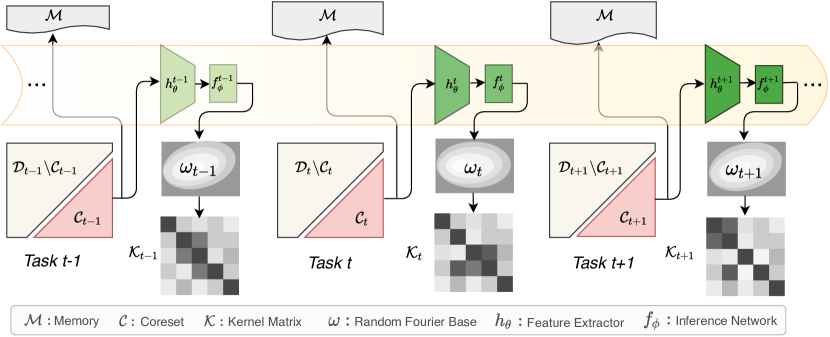
Figure 1: Overview of kernel continual learning with variational random features. For each task $t$, we use the coreset $\mathcal{C}_{t}$ to infer the random Fourier basis, which generates kernel matrix $\mathcal{K}_{t}$. The classifier for this task is constructed based on kernel ridge regression using $\mathcal{K}_{t}$. $h_{\theta}$ denotes the feature extraction network, parameterized by $\theta$, which is shared and updated when training on the task sequence. $f_{\phi}$ is the inference network, parameterized with $\phi$ for random Fourier bases, which is also shared across tasks and updated throughout learning. Memory $\mathcal{M}$ stores the coreset from each task and is used for inference only. $h_{\theta}$ and $f_{\phi}$ are jointly learned end-to-end.

In this paper, we propose kernel continual learning to deal with catastrophic forgetting in continual learning. Specifically, we propose to learn non-parametric classifiers based on kernel ridge regression. To do so, we deploy an episodic memory unit to store a subset of samples from the training data for each task, which we refer to as ‘the coreset’, and learn the classifier based on the kernel ridge regression. Kernels provide several benefits. First, the direct interference of classifiers is naturally avoided as kernels are established in a non-parametric way for each task and no classifier parameters are shared across tasks. Moreover, in contrast to existing memory replay methods, e.g., (Kirkpatrick et al., 2017; Chaudhry et al., 2019a), our kernel continual learning does not need to replay data from previous tasks when training the current task, which avoids task interference while enabling more efficient optimization. In order to achieve adaptive kernels for each task, we further introduce random Fourier features to learn kernels in a data-driven manner. Specifically, we formulate kernel continual learning with random Fourier features as a variational inference problem, where the random Fourier basis is treated as a latent variable. The variational inference formulation naturally induces a regularization term that encourages the model to learn adaptive kernels for each task from the coreset only. As a direct result, we are able to achieve more compact memory, which reduces the storage overhead.

We perform experiments on four benchmark datasets: Rotated MNIST, Permuted MNIST, Split CIFAR100 and miniImageNet. The results demonstrate the effectiveness and promise of kernel continual learning, which delivers state-of-the-art performance on all benchmarks.

2 Related Works

A fundamental problem in continual learning is catastrophic forgetting. Existing methods differ in the way they deal with this. We will briefly review them in terms of regularization, dynamic architectures and experience replay. For a more extensive overview we refer readers to the reviews by Parisi et al. (2018) and Lange et al. (2019).

Regularization methods (Kirkpatrick et al., 2017; Aljundi et al., 2018; Lee et al., 2017; Zenke et al., 2017; Kolouri et al., 2019) determine the importance of each model’s parameter for each task, which prevents the parameters from being updated for new tasks. Kirkpatrick et al. (2017), for example, specify the performance of each weight with a Fisher information matrix. Alternatively, Aljundi et al. (2018), determine parameter importance by the gradient magnitude. Naturally, these methods can also be explored from the perspective of Bayesian optimization  (Nguyen et al., 2018; Titsias et al., 2020; Schwarz et al., 2018; Ebrahimi et al., 2020; Ritter et al., 2018). For instance, Nguyen et al. (2018) introduce a regularization technique to protect their model against forgetting. Bayesian or not, all these methods address catastrophic forgetting by adding a regularization term to the main loss function. As shown by Lange et al. (2019), the penalty terms proposed in such algorithms are unable to prevent drifting in the loss landscape of previous tasks. While alleviating forgetting, the penalty term also unavoidably prevents the plasticity to absorb new information from future tasks learned over a long timescale (Hadsell et al., 2020).

Dynamic architectures (Rusu et al., 2016; Yoon et al., 2018; Jerfel et al., 2019; Li et al., 2019) allocate a subset of the model parameters for each task. This is achieved by a gating mechanism (Wortsman et al., 2020; Masse et al., 2018), or by incrementally adding new parameters to the model (Rusu et al., 2016). Incremental learning and pruning is another possibility (Mallya & Lazebnik, 2018). Given an over-parameterized model with the ability to learn quite a few tasks, Mallya & Lazebnik (2018) achieve model expansion by pruning the parameters not contributing to the performance of the current task, while keeping them available for future tasks. These methods are preferred when there is no memory usage constraint and the final model performance is prioritized. They offer an effective way to avoid task interference and catastrophic forgetting, but suffer from potentially unbounded model expansion and prevent positive knowledge transfer across tasks.

Experience replay methods (Lange et al., 2019) assume it is possible to access data from previous tasks by having a fixed-size memory or a generative model able to produce samples from old tasks (Lopez-Paz & Ranzato, 2017; Riemer et al., 2019; Rios & Itti, 2018; Shin et al., 2017; Zhang et al., 2019). Rebuffi et al. (2017) introduce a model augmented with fixed-size memory, which accumulates samples in the proximity of each class center. Chaudhry et al. (2019b) propose another memory-based model by exploiting a reservoir sampling strategy in the raw input data selection phase. Rather than storing the original samples, Chaudhry et al. (2019a) accumulate the parameter gradients during task learning. Shin et al. (2017) incorporate a generative model into a continual learning model to alleviate catastrophic forgetting by producing samples from previous tasks and retraining the model using data from both previous tasks and the current one. These papers assume that an extra neural network, such as a generative model, or a memory unit is available. Otherwise, these methods cannot be exploited. Replay-based methods benefit from a memory unit to retrain their model over previous tasks. In contrast, our proposed method only uses memory to store data as a task identifier proxy at inference time without the need of replay for training, which mitigates the optimization cost.

3 Kernel Continual Learning

3.1 Problem Statement

In the traditional supervised learning setting, a model or agent $f$ is learned to map input data from the input space to its target in the corresponding output space: $\mathcal{X}\mapsto\mathcal{Y}$, where samples $X\in\mathcal{X}$ are assumed to be drawn from the same data distribution. In the case of the image classification problem, $X$ are the images and $Y$ are associated class labels. Instead of solving a single task, continual learning aims to solve a sequence of different tasks, $T_{1},T_{2},\cdot\cdot\cdot T_{n}$, from non-stationary data distributions, where $n$ stands for the number of tasks, and each of which is an individual classification problem. A continual learner is required to continually solve each $t$ of those tasks once being trained on its labeled data, while remaining able to solve previous tasks with no or limited access to their data.

Generally, a continual learning model based on a neural network is comprised of a feature extractor $h_{\theta}$ and a classifier $f_{c}$. The feature extractor is a convolutional architecture found before the last fully connected layer, which is shared across tasks. The classifier is the last fully connected layer. We propose to learn a task-specific, non-parametric classifier based on kernel ridge regression.

We consider learning the model on the current task $t$. Given its training data $\mathcal{D}_{t}$, we choose uniformly a subset of data between existing classes in current task $t$, which is called the coreset dataset (Nguyen et al., 2018) and denoted as: $\mathcal{C}_{t}{=}{(\mathbf{x}_{i},\mathbf{y}_{i})}_{i{=}1}^{N_{c}}$. We construct the classifier $f_{c}$ based on kernel ridge regression on the coreset. Assume we have the classifier with weight $\mathbf{w}$, and the loss function of kernel ridge regression takes the following form:

$$\mathcal{L}_{\rm{krr}}(\mathbf{w})=\frac{1}{2}\sum_{i}(\mathbf{y}_{i}-\mathbf{w}^{\top}\psi(\mathbf{x}_{i}))+\frac{1}{2}\lambda||\mathbf{w}||^{2},$$ (1)

where $\lambda$ is the weight decay parameter. Based on the Representer theorem (Schölkopf et al., 2001), we have:

$$\mathbf{w}=f^{\alpha^{t}}_{c}(\cdot)=\sum^{N_{c}}_{i=1}\alpha_{i}k(\cdot,\psi(\mathbf{x}_{i})),$$ (2)

where $k(\cdot,\cdot)$ is the kernel function. Then $\alpha$ can be calculated in a closed form:

$$\alpha^{t}=Y(\lambda I+\mathcal{K})^{-1},$$ (3)

where $\alpha^{t}{=}[\alpha_{1},\cdots,\alpha_{i},\cdots,\alpha_{N_{C}}]$ and $\lambda$ is considered to be a learnable hyperparameter. The $\mathcal{K}\in R^{N_{c}\times N_{c}}$ matrix for each task is computed as $k(\mathbf{x}_{i},\mathbf{x}_{j}){=}\psi(\mathbf{x}_{i})\psi(\mathbf{x}_{j})^{\top}$. Here, $\psi(\mathbf{x}_{i})$ is the feature map of $\mathbf{x}_{i}\in\mathcal{C}_{t}$, which can be obtained from the feature extractor $h_{\theta}$.

To jointly learn the feature extractor $h_{\theta}$, we minimize the overal loss function over samples from the remaining set:

$$\sum_{(\mathbf{x}^{\prime},\mathbf{y}^{\prime})\in D_{t}\backslash\mathcal{C}_{t}}{\mathcal{L}(f^{\alpha^{t}}_{c}({\psi(\mathbf{x}^{\prime})),\mathbf{y}^{\prime}})}.$$ (4)

Here, we choose $\mathcal{L}(\cdot)$ to be the cross-entropy loss function and the predicted output $\tilde{\mathbf{y}}^{\prime}$ is computed by

$$\tilde{\mathbf{y}}^{\prime}=f^{\alpha^{t}}_{c}(\psi(\mathbf{x}^{\prime}))=\texttt{Softmax}(Y(\lambda I+\mathcal{K})^{-1}\tilde{K}),$$ (5)

where $\tilde{K}{=}\psi(X)\psi(\mathbf{x}^{\prime})^{\top}$, $\psi(X)$ denotes the feature maps of samples in the coreset, and $\texttt{Softmax}(\cdot)$ is the softmax function applied to the output of the kernel ridge regression.

In principle, we can use any (semi-)positive definite kernel, e.g., a radial basis function (RBF) kernel or a dot product linear kernel to construct the classifier. However, none of those kernels are task specific, potentially suffering from suboptimal performance, especially with limited data. Moreover, we would require a relatively large coreset to obtain informative and discriminative kernels for satisfactory performance. To address this, we further introduce random Fourier features to learn data-driven kernels, which have previously demonstrated success in regular learning tasks (Bach et al., 2004; Sinha & Duchi, 2016; Carratino et al., 2018; Zhen et al., 2020). Data-driven kernels using random Fourier features provides an appealing technique to learn strong classifiers with a relatively small memory footprint for continual learning based on episodic memory.

3.2 Variational Random Features

One of the key ingredients when finding a mapping function in non-parametric approaches, such as kernel ridge regression, is the kernel function. Rahimi & Recht (2007) introduced an algorithm to approximate translation-invariant kernels using explicit feature maps, which is theoretically underpinned by Bochner’s theorem (Rudin, 1962).

Theorem 1 (Bochner’s Theorem)

A continuous, real valued, symmetric and shift-invariant function $\mathrm{k}\left(\mathbf{x},\mathbf{x}^{\prime}\right)=\mathrm{k}(\mathbf{x}-\mathbf{x}^{\prime})$ on $\mathbb{R}^{\mathrm{d}}$ is a positive definite kernel if and only if it is the Fourier transform $p(w)$ of a positive finite measure such that:

$$\mathrm{k}\left(\mathbf{x},\mathbf{x}^{\prime}\right)= \int_{\mathbb{R}^{d}}e^{i\omega^{\top}\left(\mathbf{x}-\mathbf{x}^{\prime}\right)}dp(\boldsymbol{\omega})=\mathbb{E}_{\omega}\left[\zeta_{\omega}(\mathbf{x})\zeta_{\omega}\left(\mathbf{x}^{\prime}\right)^{*}\right]$$ (6)

$$\text{ where }\zeta_{w}(\mathbf{x})=e^{i\omega^{\top}\mathbf{x}}.$$

With a sufficient number of samples $\omega$ drawn from $p(\omega)$, we can achieve an unbiased estimation of $\mathrm{k}\left(\mathbf{x},\mathbf{x}^{\prime}\right)$ by $\zeta_{w}(\mathbf{x})\zeta_{w}(\mathbf{x})^{*}$ (Rahimi & Recht, 2007).

Based on Theorem 1, we draw $D$ sets of samples: $\{{\omega_{i}}\}_{i=1}^{D}$ and $\{{b_{i}}\}_{i=1}^{D}$ from a normal distribution and uniform distribution (with a range of [$0$, $2\pi$]), respectively, and construct the random Fourier features (RFFs) for each data point $\mathbf{x}$ using the formula:

$$\psi(\mathbf{x})=\frac{1}{\sqrt{D}}\left[\cos\left(\boldsymbol{\omega}_{1}^{\top}\mathbf{x}+b_{1}\right),\cdots,\cos\left(\boldsymbol{\omega}_{D}^{\top}\mathbf{x}+b_{D}\right)\right].$$ (7)

Having the random Fourier features, we calculate the kernel matrix by $\mathrm{k}\left(\mathbf{x},\mathbf{x}^{\prime}\right){=}\psi(\mathbf{x})\psi(\mathbf{x}^{\prime})^{\top}$.

Traditionally the shift-invariant kernel is constructed based on random Fourier features, where the Fourier basis is drawn from a Gaussian distribution transformed from a pre-defined kernel. This results in kernels that are agnostic to the task. In continual learning, however, tasks are provided sequentially from non-stationary data distributions, which makes it suboptimal to share the same kernel function across tasks. To address this problem, we propose to learn task-specific kernels in a data-driven manner. This is even more appealing in continual learning as we would like to learn informative kernels using a coreset of a minimum size. We formulate it as a variational inference problem, where we treat the random basis $\omega$ as a latent variable.

Evidence Lower Bound

From the probabilistic perspective, we would like to maximize the following conditional predictive log-likelihood for the current task $t$:

$$\max_{p}\sum_{(\mathbf{x},\mathbf{y})\in\mathcal{D}_{t}\backslash\mathcal{C}_{t}}\ln p(\mathbf{y}|\mathbf{x},\mathcal{D}_{t}\backslash\mathcal{C}_{t}),$$ (8)

which amounts to making maximally accurate predictions on $\mathbf{x}$ based on $\mathcal{D}_{t}\backslash\mathcal{C}_{t}$.

By introducing the random Fourier basis $\omega$ into Eq. (8), which is treated as a latent variable, we have:

$$\max_{p}\sum_{(\mathbf{x},\mathbf{y})\in\mathcal{D}_{t}\backslash\mathcal{C}_{t}}\ln\int p(\mathbf{y}|\mathbf{x},\omega,\mathcal{D}_{t}\backslash\mathcal{C}_{t})p_{\gamma}(\omega|\mathcal{D}_{t}\backslash\mathcal{C}_{t})d\omega.$$ (9)

The intuition is that we can use data to infer the distribution over the latent variable $\omega$ whose prior is conditioned on the data. We combine the data and $\omega$ to generate kernels to classify $\mathbf{x}$ based on kernel ridge regression. We can also simply place an uninformative prior of a standard Gaussian distribution over the latent variable $\omega$, which will be investigated in our experiments.

It is intractable to directly solve for the true posterior $p(\omega|\mathbf{x},\mathbf{y},\mathcal{D}_{t}\backslash\mathcal{C}_{t})$ over $\omega$. We therefore introduce a variational posterior $q_{\phi}(\omega|\mathcal{C}_{t})$ conditioned solely on the coreset $\mathcal{C}_{t}$ because the coreset will be stored as episodic memory for the inference of each corresponding task.

By incorporating the variational posterior into Eq. (9) and applying Jensen’s inequality, we establish the evidence lower bound (ELBO) as follows:

$$\ln p(\mathbf{y}|\mathbf{x},\mathcal{D}_{t}\backslash\mathcal{C}_{t}) \geq\mathbb{E}_{q_{\phi}(\boldsymbol{\omega}|\mathcal{C}_{t})}\big{[}\ln p(\mathbf{y}|\mathbf{x},\boldsymbol{\omega},\mathcal{D}_{t}\backslash\mathcal{C}_{t})\big{]}$$ (10)

$$-D_{\mathrm{KL}}\big{[}q_{\phi}(\boldsymbol{\omega}|\mathcal{C}_{t})\|p_{\gamma}(\boldsymbol{\omega}|\mathcal{D}_{t}\backslash\mathcal{C}_{t})\big{]}$$

$$=\mathcal{L}_{\mathrm{ELBO}}.$$

Therefore, maximizing the ELBO amounts to maximizing the conditional log-likelihood in Eq. (8). The detailed derivation is provided in the supplementary materials.

Empirical Objective Function

In the continual learning setting, we would like the model to be able to make predictions based solely on the coreset $\mathcal{C}_{t}$ stored in the memory. That is, the conditional log-likelihood should be conditioned on the coreset only. Based on the ELBO in Eq. (15) we establish the following empirical objective function which, is minimized by our overall training procedure:

$$\tilde{\mathcal{L}}_{\mathrm{ELBO}} =\frac{1}{T}\sum_{t=1}^{T}\Big{[}\sum_{(\mathbf{x},\mathbf{y})\in\mathcal{D}_{t}\backslash\mathcal{C}_{t}}\frac{1}{L}\sum^{L}_{\ell=1}\big{[}\ln p(\mathbf{y}|\mathbf{x},\boldsymbol{\omega}^{(\ell)},\mathcal{C}_{t})\big{]}$$ (11)

$$-D_{\mathrm{KL}}\big{[}q_{\phi}(\boldsymbol{\omega}|\mathcal{C}_{t})\|p_{\gamma}(\boldsymbol{\omega}|\mathcal{D}_{t}\backslash\mathcal{C}_{t})\big{]}\Big{]},$$

where, in the first term, we employ the Monte Carlo method to draw samples from the variational posterior $q(\omega|\mathcal{C}_{t})$ to estimate the log-likelihood, and $L$ is the number of Monte Carlo samples. In the second term, the conditional prior serves as a regularizer that ensures the inferred random Fourier basis will always be relevant to the current task. Minimizing the Kullback Leibler (KL) divergence forces the distribution of random Fourier bases, as inferred from the coreset, to be close to the one from the training set. Moreover, the KL term enables us to generate informative kernels adapted to each task using relatively small memory.

In practice, the conditional distributions $q_{\phi}(\boldsymbol{\omega}|\mathcal{C}_{t})$ and $p_{\gamma}(\boldsymbol{\omega}|\mathcal{D}_{t}\backslash\mathcal{C}_{t})$ are assumed to be Gaussian. We implement them by using the amortization technique (Kingma & Welling, 2014). That is, we use multilayer perceptrons to generate the distribution parameters, $\mu$ and $\sigma$, by taking the conditions as input. In our experiments, we deploy two separate amortization networks, referred to as the inference network $f_{\phi}$ for the variational posterior and the prior network $f_{\gamma}$ for the prior. In addition, to demonstrate the effectiveness of data-driven kernels, we also implement a variant of variational random features by replacing the conditional prior in Eq. (11) with an uninformative one, i.e., an isotropic Gaussian distribution $\mathcal{N}(0,\rm{I})$. In this case, kernels are also learned in a data-driven way from the coreset without being regulated by the training data from the task.

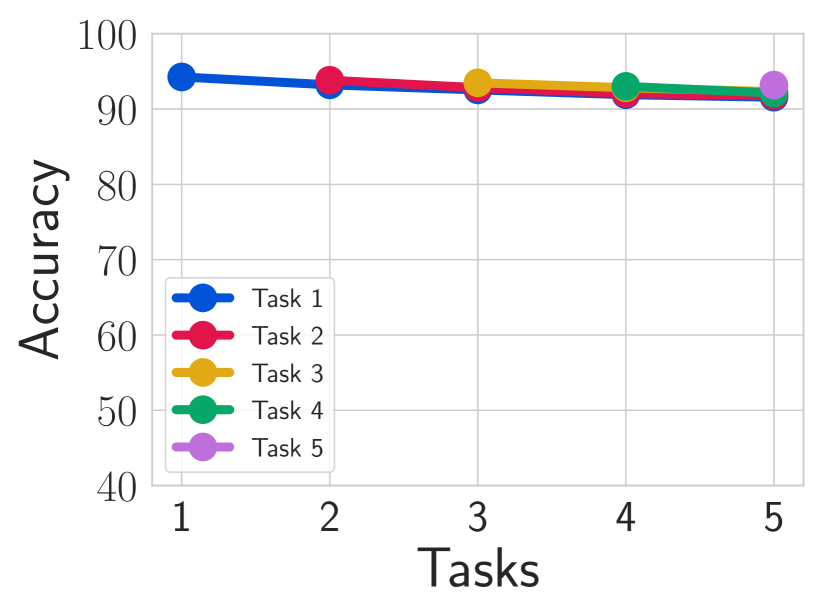
(a) Permuted MNIST

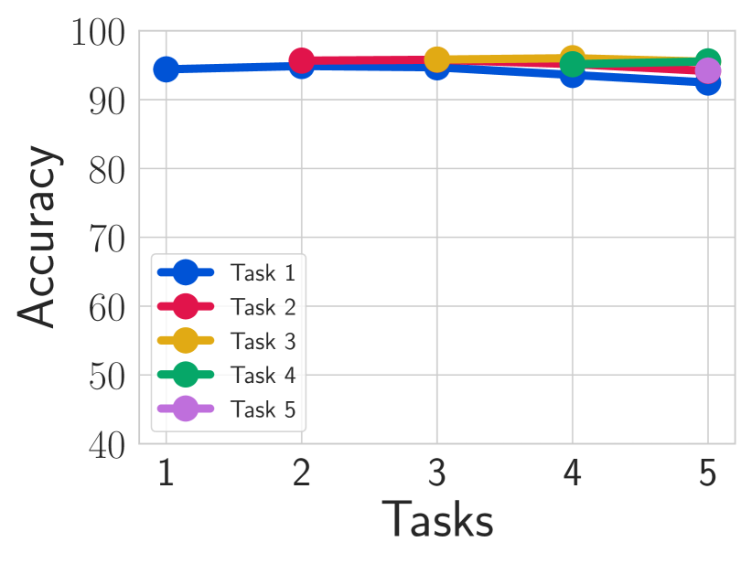
(b) Rotated MNIST

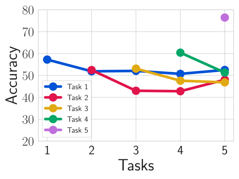
(c) Split CIFAR100

Figure 2: Effectiveness of kernels. Accuracy of kernel continual learning by variational random features for the first five tasks on three benchmarks. Note the limited decline in accuracy as the number of tasks increase.

4 Experiments

We conduct our experiments on four benchmark datasets for continual learning. We perform thorough ablation studies to demonstrate the effectiveness of kernels for continual learning as well as the benefit of variational random features in learning data-driven kernels.

4.1 Datasets

Permuted MNIST Following (Kirkpatrick et al., 2017), we generate 20 different MNIST datasets. Each dataset is created by a special pixel permutation of the input images, without changing their corresponding labels. Each dataset has its own permutation by owning a random seed.

Rotated MNIST Similar to Permuted MNIST, Rotated MNIST has 20 tasks (Mirzadeh et al., 2020). Each task’s dataset is a specific random rotation of the original MNIST dataset, e.g., the dataset for task $1$, task $2$, and task $3$ are the original MNIST dataset, a 10-degree rotation, and a 20-degree rotation, respectively. In other words, each task’s dataset is a 10-degree rotation of the previous task’s dataset.

Split CIFAR100 Zenke et al. (2017) created this benchmark by dividing the CIFAR100 dataset into 20 sections. Each section represents $5$ out of $100$ labels (without replacement) from CIFAR100. Hence, it contains $20$ tasks and each task is a $5$-way classification problem.

Split miniImageNet Similar to Split CIFAR100, the miniImageNet benchmark (Vinyals et al., 2016) contains 100 classes, and is a subset of the original ImageNet dataset (Russakovsky et al., 2015). It has 20 disjoint tasks, each of which task contains 5 classes.

4.2 Evaluation Metrics

We follow the common conventions in continual learning  (Chaudhry et al., 2018; Mirzadeh et al., 2020), and report the average accuracy and average forgetting metrics.

Average Accuracy This score shows the model accuracy after training over $t$ consecutive tasks are finished. It is formulated as follows:

$$\mathrm{A}_{t}=\frac{1}{t}\sum_{i=1}^{t}\mathrm{a}_{t,i},$$ (12)

where $\mathrm{a}_{t,i}$ refers to the model performance on task $i$ after being trained on task $t$.

Average Forgetting This metric measures the decline in accuracy for each task, according to the highest accuracy and the final accuracy reached after model training is finished. It is formulated as follows:

$$\mathrm{F}=\frac{1}{T-1}\sum_{i=1}^{T-1}\rm{max}_{1,...,T-1}(\mathrm{a}_{t,i}-\mathrm{a}_{T,i}).$$ (13)

Taken together, the two metrics allow us to asses how well a continual learner achieves its classification target while overcoming forgetting.

4.3 Implementation Details

Our kernel continual learning contains three networks: a shared backbone $h_{\theta}$, a posterior network $f_{\phi}$, and a prior network $f_{\gamma}$. An overview of our implementation is provided in the supplementary materials. For the Permuted MNIST and Rotated MNIST benchmarks, $h_{\theta}$ contains only two hidden layers, each of which has $256$ neurons, followed by a ReLU activation function. For Split CIFAR100, we use a ResNet18 architecture similar to Mirzadeh et al. (2020), and for miniImageNet, we have a ResNet18 similar to  Chaudhry et al. (2020). With regard to the $f_{\gamma}$ and $f_{\phi}$ networks, we adopt three hidden layers followed by an ELU activation function (Gordon et al., 2019). The number of neurons in each layer depends on the benchmark. On Permuted MNIST and Rotated MNIST, there are $256$ neurons per layer, and we use $160$ and $512$ for Split CIFAR100 and miniImageNet, respectively. For fair comparisons, the model is trained for only one epoch per task, that is, each sample in the dataset is observed only once. The batch size is set to 10. Other optimization techniques, such as weight-decay, learning rate decay, and dropout are set to the same values as in (Mirzadeh et al., 2020). The model is implemented in Pytorch (Paszke et al., 2019). All our code will be released.

4.4 Results

We first provide a set of ablation studies for our proposed method. Then, the performance of our method is compared against other continual learning methods (see the supplementary materials for more details about each ablation).

Effectiveness of kernels

To demonstrate the effectiveness of kernels for continual learning, we establish classifiers based on kernel ridge regression using commonly used linear, polynomial, radial basis function (RBF) kernels, and our proposed variational random Fourier features. We report results on Split CIFAR100, where we sample five different random seeds. For each random seed, the model is trained over different kernels. Finally, the result for each kernel is estimated by averaging over the corresponding random seeds. For fair comparison, all kernels are computed using the same coreset of size $20$.

The results are shown in Table 1. All kernels perform well: the radial basis function (RBF) obtains a modest average accuracy in comparison to other basic kernels such as the linear and polynomial kernels. The linear and polynomial kernels perform similarly. The kernels obtained from variational random features (VRFs) achieve the best performance in comparison to other kernels, and they work better than its uninformative counterpart. This emphasizes that the prior incorporated in VRFs is more informative because its prior is data-driven.

Regarding VRFs, Figure 2 demonstrates the change of each task’s accuracy on Permuted MNIST, Rotated MNIST and Split CIFAR100. It is also worth mentioning that the classifiers based on those kernels are non-parametric, enabling them to systematically avoid task interference in classifiers. Thanks to the non-parametric nature of the classifiers based on kernels, our method is flexible and able to naturally deal with a more challenging setting under a different numbers of classes (which we refer to as ‘varied ways’). To demonstrate this, we conduct experiments with a varying number of classes in each task using VRFs. The results on Split CIFAR100 and Split miniIMageNet are shown in Table 2. Kernel continual learning results in slightly lower accuracy on Split CIFAR100, but leads to an improvement over the traditional fixed ways evaluation on Split miniImageNet.

Table 1: Effectiveness of kernels on Split CIFAR100. All kernels perform well, but the simple linear kernel performs better than the RBF kernel. The adaptive kernels based on the random Fourier features achieve the best performance, indicating the advantage of data-driven kernels.

	Split CIFAR100
Kernel	Accuracy	Forgetting
RBF	56.86 $\pm$ 1.67	0.03 $\pm$ 0.008
Linear	60.88 $\pm$ 0.64	0.05 $\pm$ 0.007
Polynomial	60.96 $\pm$ 1.19	0.03 $\pm$ 0.004
VRF (uninformative prior)	62.46 $\pm$ 0.93	0.05 $\pm$ 0.004
VRF	62.70 $\pm$ 0.89	0.06 $\pm$ 0.008

Table 2: Effectiveness of VRF kernel for variable-way scenario on Split CIFAR100 and Split miniImageNet. In this scenario, instead of covering a fixed number of five classes per task from Split CIFAR100 and Split miniImageNet, a task is able to cover a more flexible number of classes in the range $[3,15]$. By doing so, the experimental setting is more realistic. Even in this case, our proposed method is effective, as indicated by the performance improvement of miniImageNet.

	Split CIFAR100		Split miniImageNet
	Accuracy	Forgetting	Accuracy	Forgetting
Fixed Ways	64.02	0.05	51.89	0.06
Varied Ways	61.00$\pm$ 1.80	0.05$\pm$ 0.01	53.90$\pm$ 2.95	0.05$\pm$ 0.01

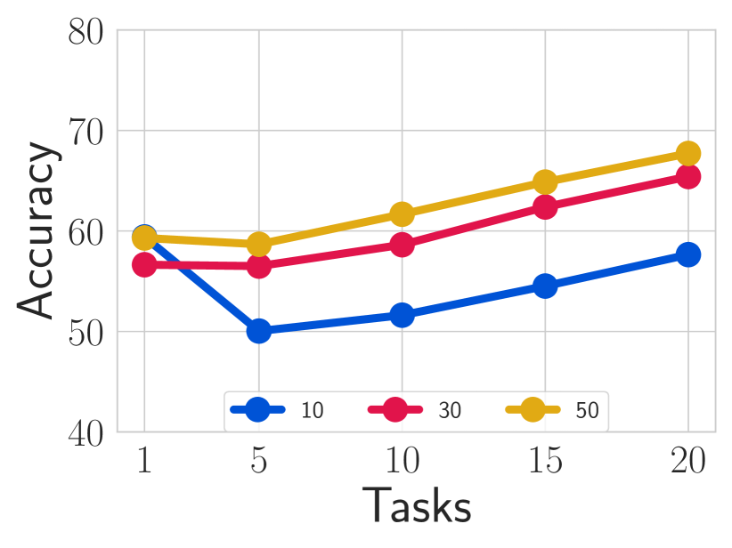
(a) Split CIFAR100

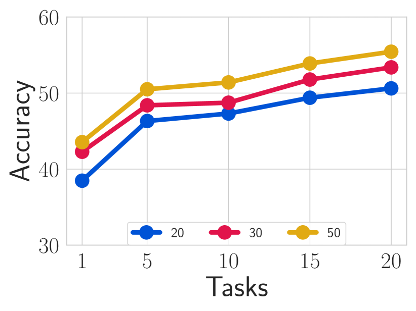
(b) Split miniImageNet

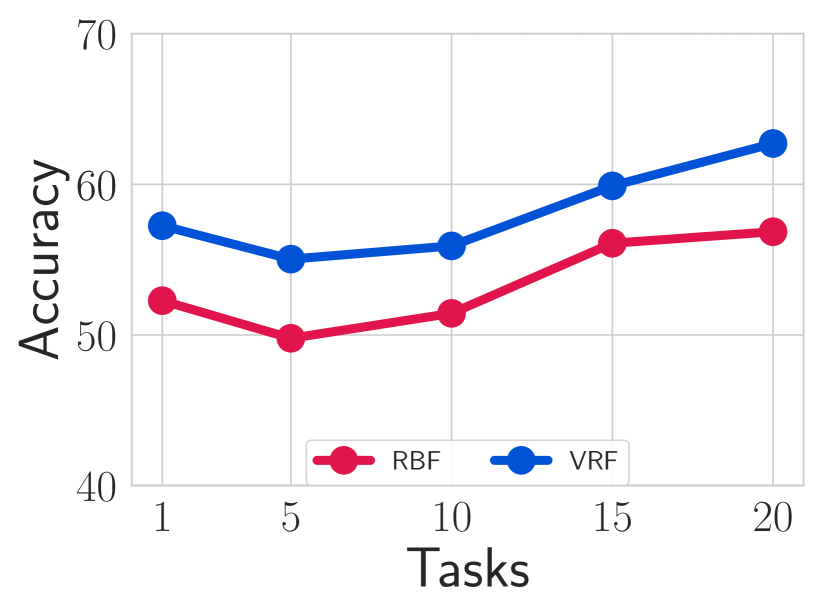
(c) RBF vs. VRF on Split CIFAR100

Figure 3: Influence of number of tasks. The average accuracies of kernel continual learning by variational random features for $20$ tasks under three different coreset sizes are illustrated on Split CIFAR100 (a) and Split miniImageNet (b). Moreover, in figure (c), we show the average accuracy of two VRF and RBF kernels. As show in all figures, our proposed kernel continual learning is improved when observing more tasks.

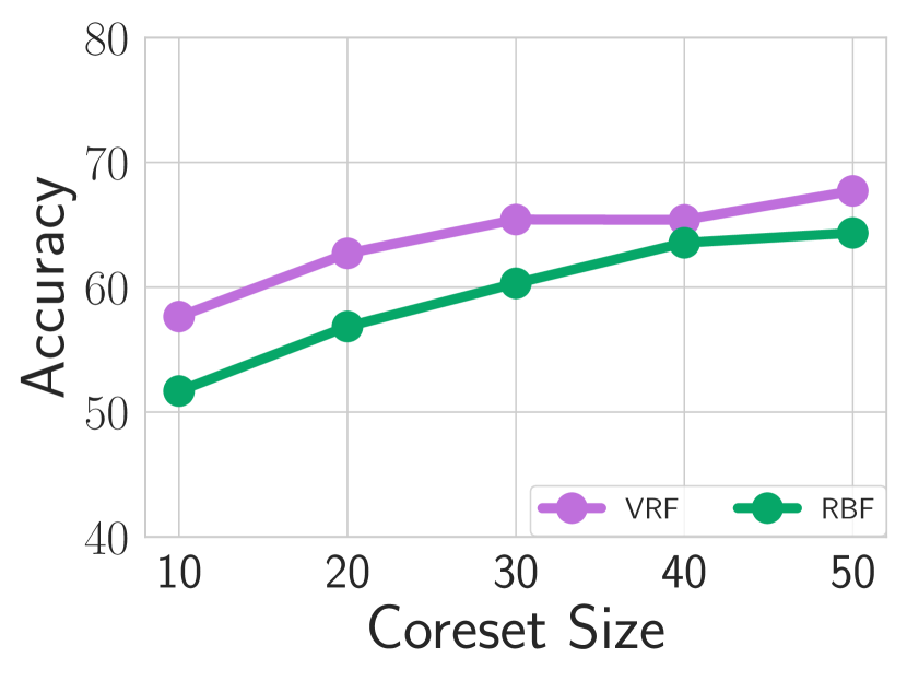
Figure 4: Memory benefit of Variational Random Features. To achieve similar performance, variational random features need a smaller coreset size compared to RBF kernels, showing the benefit of variational random features for kernel continual learning.

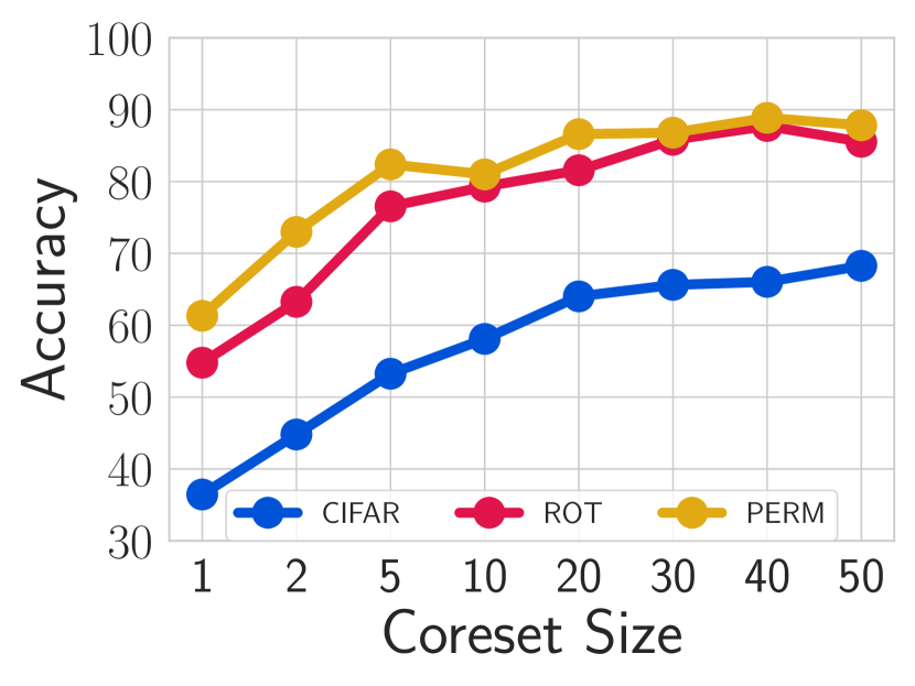
Figure 5: How much inference memory? Enlarging the coreset size of the VRF kernel leads to improvement in performance on all datasets. The more challenging the dataset, the more memory size helps.

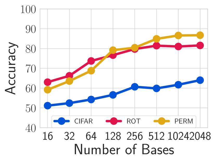
Figure 6: How many Random Bases? In general, a larger number of random Fourier bases consistently improves the performance on all benchmarks. With the relatively small number of $256$ bases, our variational random features can deliver good performance.

Table 3: How much inference memory? Increasing the coreset size has only a minimal impact on time complexity at inference.

	Split CIFAR100
	5	10	20	40
Time (s)	0.0017	0.0017	0.0017	0.0018

Table 4: How may Random Bases? Increasing the number of Random Bases leads to an increased time complexity at inference.

	Split CIFAR100
	256	512	1024	2048
Time (s)	0.0014	0.0015	0.0015	0.0017

Influence of Number of Tasks

Next we ablate the robustness of our proposal when the number of tasks increase. We report results with three different coreset sizes on Split CIFAR100 and Split miniImageNet in Figure 3 (a) and (b). As can be seen, our method achieves increasingly better performance as the number of tasks increases, indicating that knowledge is transferred forward from previous tasks to future tasks. The observed positive transfer is likely due to the shared parameters in the feature extractors and amortization networks, as they allow knowledge to be transferred across tasks. We again show a comparison between variational random features and a predefined RBF kernel in Figure 3 (c). The performance for variational random features increases faster than the RBF kernel when observing more tasks. This might be due to the amortization network shared among tasks, which enables knowledge to be transferred across tasks as well, indicating the benefit of learning data-driven kernels by our variational random features.

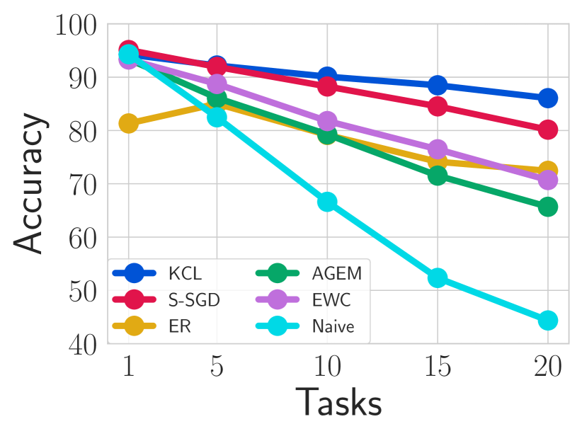
(a) Permuted MNIST

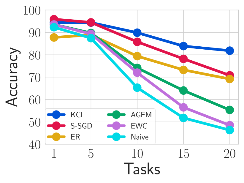
(b) Rotated MNIST

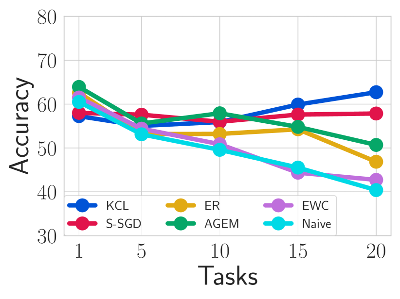
(c) Split CIFAR100

Figure 7: Comparison between the state of the art and our kernel continual learning by variational random features over 20 consecutive tasks, in terms of average accuracy. Our model consistently performs better than other methods with less accuracy drop on Rotated and Permuted MNIST and, further, the performance even starts to increase when observing more tasks on the challenging Split CIFAR100 dataset.

Table 5: Comparison to the state-of-the-art. Results for other methods on Permuted MNIST, Rotated MNIST and Split CIFAR100 are adopted from Mirzadeh et al. (2020). For Split miniImageNet results are from Chaudhry et al. (2020).We include columns denoting if and when memory is used. In all cases, kernel continual learning is best.

Method	Memory		Permuted MNIST		Rotated MNIST		Split CIFAR100		Split miniImageNet
	If	When	Accuracy	Forgetting	Accuracy	Forgetting	Accuracy	Forgetting	Accuracy	Forgetting
Lower Bound: Naive-SGD (Mirzadeh et al., 2020)	✗	-	44.4$\pm$2.46	0.53$\pm$0.03	46.3$\pm$1.37	0.52$\pm$0.01	40.4 $\pm$2.83	0.31$\pm$0.02	36.1$\pm$ 1.31	0.24$\pm$ 0.03
EWC (Kirkpatrick et al., 2017)	✗	-	70.7$\pm$1.74	0.23$\pm$0.01	48.5$\pm$1.24	0.48$\pm$0.01	42.7$\pm$1.89	0.28$\pm$0.03	34.8$\pm$ 2.34	0.24 $\pm$ 0.04
AGEM (Chaudhry et al., 2019a)	✓	Train	65.7$\pm$0.51	0.29$\pm$0.01	55.3$\pm$1.47	0.42$\pm$0.01	50.7$\pm$2.32	0.19$\pm$0.04	42.3$\pm$ 1.42	0.17$\pm$ 0.01
ER-Reservoir (Chaudhry et al., 2019b)	✓	Train	72.4$\pm$0.42	0.16$\pm$0.01	69.2$\pm$1.10	0.21$\pm$0.01	46.9$\pm$0.76	0.21$\pm$0.03	49.8$\pm$ 2.92	0.12$\pm$ 0.01
Stable SGD (Mirzadeh et al., 2020)	✗	-	80.1$\pm$0.51	0.09$\pm$0.01	70.8$\pm$0.78	0.10$\pm$0.02	59.9$\pm$1.81	0.08$\pm$0.01	-	-
Kernel Continual Learning	✓	Test	85.5$\pm$0.78	0.02$\pm$0.00	81.8$\pm$0.60	0.01$\pm$0.00	62.7$\pm$0.89	0.06$\pm$0.01	53.3$\pm$ 0.57	0.04$\pm$ 0.00
Upper Bound: multi-task learning (Mirzadeh et al., 2020)	✗	-	86.5$\pm$0.21	0.0	87.3$\pm$0.47	0.0	64.8$\pm$0.72	0.0	65.1	0.0

Memory benefit of Variational Random Features

To further demonstrate the memory benefit of data-driven kernel learning, we compare variational random features with a predefined RBF kernel in Figure 6. We consider five different coreset sizes. Variational random features exceed the RBF kernel consistently. For instance, With a smaller coreset size of 20, variational random features can achieve similar performance to the RBF kernel with a larger coreset size of 40. This demonstrates that learning task-specific kernels in a data driven way enables us to use less memory than with a pre-defined kernel.

How much inference memory?

Since kernel continual learning does not need to replay and only uses memory for inference, the coreset size plays a crucial role. We therefore ablate its influence on Rotated MNIST, Permuted MNIST, and Split CIFAR100 by varying the coreset size as 1, 2, 5, 10, 20, 30, 40, and 50. Here, the number of random bases is set to 1024 for Rotated MNIST and Permuted MNIST, and 2048 for Split CIFAR100. The results in Figure 10 show that increasing the coreset size from 1 to 5 results in a steep accuracy increase for all datasets. This continues depending on the difficulty of the dataset. For Split CIFAR100, the results start to saturate after a coreset size of 20. This is expected as increasing the number of samples in a coreset allows us to better infer the random Fourier bases with more data from the task, therefore resulting in more representative and descriptive kernels. In the remaining experiments we use a coreset size of $20$ for Rotated MNIST, Permuted MNIST and Split CIFAR100, and a coreset size of $30$ for miniImageNet (see supplementary materials). We also ablate the effect of the coreset size on time complexity in Table 3. Indeed, it shows that increasing the coreset size only comes with a limited cost increase at inference time.

How many Random Bases?

When approximating VRF kernels the number of random Fourier bases is a important hyperparameter. In principle, a larger number of random Fourier bases should yield a better approximation of kernels, leading to better classification accuracy. Here, we investigate its effect on the continual learning accuracy. Results with different numbers of bases are shown in Figure 10 on Rotated MNIST, Permutated MINST and Split CIFAR100. As expected, the performance increases with a larger number of random Fourier bases, but with a relatively small number of $256$ bases, our method already performs well on all datasets. Table 4 further shows the impact of the number of random bases on time complexity. It highlights that increasing the number of random bases comes with an increasing computation time for the model at inference time.

Comparison to the state-of-the-art

We compare kernel continual learning with alternative methods on the four benchmarks. The accuracy and forgetting scores in Table 5 for Rotated MNIST, Permuted MNIST and Split CIFAR100 are all adopted from (Mirzadeh et al., 2020), and results for miniImageNet are from (Chaudhry et al., 2020). The “if” column indicates whether a model utilizes memory and if so, the “when” column denotes whether the memory data are used during training time or test time. Our method achieves better performance in terms of average accuracy and average forgetting. Moreover, compared to memory-based methods such as A-GEM (Chaudhry et al., 2019a) and ER-Reservoir (Chaudhry et al., 2019b), which replay over previous tasks (when $=$ Train), kernel continual learning does not require replay, enabling our method to be efficient during training time. Further, for the most challenging miniImageNet dataset, kernel continual learning also performs better than other methods, both in terms of accuracy and forgetting. In Figure 7, we compare our kernel continual learning by variational random features with other methods in terms of average accuracy over 20 consecutive tasks. Our method performs consistently better. It is worth noting that on the relatively challenging Split CIFAR100 dataset, the accuracy of our method drops a bit at the beginning but starts to increase when observing more tasks. This indicates a positive forward transfer from previous tasks to future tasks. All hyperparameters for reproducing the results in Figure 7 and Table 5 are provided in the supplementary materials.

5 Conclusion

In this paper, we introduce kernel continual learning, a simple but effective variation of continual learning with kernel-based classifiers. To mitigate catastrophic forgetting, instead of using shared classifiers across tasks, we propose to learn task-specific classifiers based on kernel ridge regression. Specifically, we deploy an episodic memory unit to store a subset of training samples for each task, which is referred to as the coreset. We formulate kernel learning as a variational inference problem by treating random Fourier bases as the latent variable to be inferred from the coreset. By doing so, we are able to generate an adaptive kernel for each task while requiring a relatively small memory size. We conduct extensive experiments on four benchmark datasets for continual learning. Our thorough ablation studies demonstrate the effectiveness of kernels for continual learning and the benefits of variational random features in learning data-driven kernels for continual learning. Our kernel continual learning already achieves state-of-the-art performance on all benchmarks, while opening up many other possible connections between kernel methods and continual learning.

6 Appendix

In Section 6.1, we provide the detailed derivation of the Evidence Lower Bound (ELBO) of our variational random features for kernel continual learning. In Section 6.2, we illustrate our proposed model in detail, explaining each part. Moreover, for all kernels, e.g., Linear, Polynomial, and Radial Basis Function, we discuss how the main architecture is changed accordingly. In Section 6.3, all hyperparamters are listed in a table in order to reproduce the paper results. Finally, in Section 6.4, we include additional ablation results on miniImageNet for the size of inference memory and number of Random Bases.

6.1 Derivation of Evidence Lower Bound

Our proposed objective in equation 10 is derived as follows:

$$\ln p(\mathbf{y}|\mathbf{x},\mathcal{D}_{t}\backslash\mathcal{C}_{t}) =\ln\Big{[}\int p(\mathbf{y}|\mathbf{x},\boldsymbol{\omega},\mathcal{D}_{t}\backslash\mathcal{C}_{t})p(\boldsymbol{\omega}|\mathcal{D}_{t}\backslash\mathcal{C}_{t})d\boldsymbol{\omega}\Big{]}$$ (14)

$$=\ln\Big{[}\int p(\mathbf{y}|\mathbf{x},\boldsymbol{\omega},\mathcal{D}_{t}\backslash\mathcal{C}_{t})p(\boldsymbol{\omega}|\mathcal{D}_{t}\backslash\mathcal{C}_{t})\frac{q_{\phi}(\boldsymbol{\omega}|\mathcal{C}_{t})}{q_{\phi}(\boldsymbol{\omega}|\mathcal{C}_{t})}d\boldsymbol{\omega}\Big{]}$$

$$=\ln\Big{[}\mathbb{E}_{q_{\phi}(\boldsymbol{\omega}|\mathcal{C}_{t})}{\frac{p(\mathbf{y}|\mathbf{x},\boldsymbol{\omega},\mathcal{D}_{t}\backslash\mathcal{C}_{t})p(\boldsymbol{\omega}|\mathcal{D}_{t}\backslash\mathcal{C}_{t})}{q_{\phi}(\boldsymbol{\omega}|\mathcal{C}_{t})}}\Big{]}.$$

By applying Jensen’s inequality, we have

$$\ln p(\mathbf{y}|\mathbf{x},\mathcal{D}_{t}\backslash\mathcal{C}_{t}) \geq\mathbb{E}_{q_{\phi}(\boldsymbol{\omega}|\mathcal{C}_{t})}\Big{[}\ln{\frac{p(\mathbf{y}|\mathbf{x},\boldsymbol{\omega},\mathcal{D}_{t}\backslash\mathcal{C}_{t})p(\boldsymbol{\omega}|\mathcal{D}_{t}\backslash\mathcal{C}_{t})}{q_{\phi}(\boldsymbol{\omega}|\mathcal{C}_{t})}}\Big{]}$$ (15)

$$=\mathbb{E}_{q_{\phi}(\boldsymbol{\omega}|\mathcal{C}_{t})}\Big{[}\ln{p(\mathbf{y}|\mathbf{x},\boldsymbol{\omega},\mathcal{D}_{t}\backslash\mathcal{C}_{t})}+\ln{\frac{p(\boldsymbol{\omega}|\mathcal{D}_{t}\backslash\mathcal{C}_{t})}{q_{\phi}(\boldsymbol{\omega}|\mathcal{C}_{t})}}\Big{]}$$

$$=\mathbb{E}_{q_{\phi}(\boldsymbol{\omega}|\mathcal{C}_{t})}\Big{[}\ln{p(\mathbf{y}|\mathbf{x},\boldsymbol{\omega},\mathcal{D}_{t}\backslash\mathcal{C}_{t})}\Big{]}+\mathbb{E}_{q_{\phi}(\boldsymbol{\omega}|\mathcal{C}_{t})}\Big{[}\ln{\frac{p(\boldsymbol{\omega}|\mathcal{D}_{t}\backslash\mathcal{C}_{t})}{q_{\phi}(\boldsymbol{\omega}|\mathcal{C}_{t})}}\Big{]}$$

$$=\mathbb{E}_{q_{\phi}(\boldsymbol{\omega}|\mathcal{C}_{t})}\Big{[}\ln{p(\mathbf{y}|\mathbf{x},\boldsymbol{\omega},\mathcal{D}_{t}\backslash\mathcal{C}_{t})}\Big{]}-D_{\mathrm{KL}}\big{[}q_{\phi}(\boldsymbol{\omega}|\mathcal{C}_{t})\|p_{\gamma}(\boldsymbol{\omega}|\mathcal{D}_{t}\backslash\mathcal{C}_{t})\big{]}$$

$$=\mathcal{L}_{\mathrm{ELBO}}.$$

6.2 Model Details

We provide the computational graph of our kernel continual learning with variational random features in Figure 8. Our method consists of three networks. $h_{\theta}$ is the backbone network shared across different tasks to extract general features. $f_{\phi}$ and $f_{\gamma}$ are two amortized networks to estimate the posterior and prior distributions over $\omega$. $q$ and $p$ refer to posterior and prior distributions. $r_{x}$ are features extracted over samples drawn from $D\backslash C$. These features are l2-normalized as well as average pooled over samples in the batch.

On the left, we show the posterior and the priors generated in the sequence of tasks. On the right, the inference model is depicted. To predict a label for a given query sample, first, the input images and its corresponding coreset are forwarded through $h_{\theta}$ and their features are computed: $r_{x}^{t}$ and $r_{c}^{t}$. Next, we feed $r_{c}^{t}$ through $f_{\phi}$ and estimate the posterior distribution over $q_{\phi}(\omega\mid\mathcal{C}_{t})$. Then, we create the random Fourier bases $\omega_{t}$ by drawing samples from estimated posterior distribution. Having random bases for the current task $t$, $\omega_{t}$, as well as $r_{x}^{t}$ and $r_{c}^{t}$, random Fourier features related the query input $\psi(r_{x}^{t})$ and coreset data $\psi(r_{c}^{t})$ are estimated. Each kernel, $K$ and $\tilde{K}$, is estimated using its corresponding random Fourier features and $\mathrm{k}\left(\mathbf{x},\mathbf{x}^{\prime}\right){=}\psi(\mathbf{x})\psi(\mathbf{x}^{\prime})^{\top}$. Based on Eq. (5) in the main manuscript, these two estimated kernels are used to predict the output labels for given query samples.

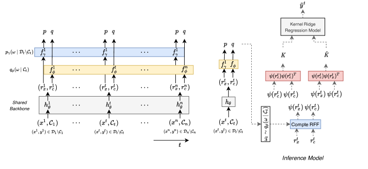
Figure 8: Kernel continual learning model with variational random features.

Note that for the variant of our variational random features with an uninformative prior. the prior network is removed and the prior is set to a standard Gaussian distribution. In addition, by using linear, polynomial, and radial basis function kernels, neither the prior network nor the posterior network is used.

6.3 Hyperparameters

We provide the detailed hyperparameter settings in Table 6, which are used to to generate Figure 7 and Table 3 in the main paper for each dataset.

Table 6: Hyperparameters used to generate results in Figure 7 and Table 3.

Method	Permuted MNIST	Rotated MNIST	Split CIFAR100	Split miniImageNet
Batch Size	10	10	10	10
Learning Rate (LR)	0.1	0.1	0.3	0.3
LR Decay Factor	0.8	0.8	0.95	0.95
Momentum	0.8	0.8	0.8	0.8
Dropout	0.5	0.5	0.02	0.02
Coreset Size	20	20	20	30
Number of Bases	1024	1024	2048	2048
Number of Tasks	20	20	20	20
Tau	0.01	0.01	0.01	0.01

6.4 Additional ablation results on miniImageNet

We provide additional ablation results on the miniImageNet dataset. We report the influence of the inference memory and the number of Random bases. Figure 10 shows increasing the coreset size from $1$ to $20$, improves average accuracy consistently. It saturates between $20$ to $40$. By enlarging the coreset size to 50, model performance increases again. In Table 3 in the main paper the results related to miniImageNet are reported based on a coreset size of 30. Figure 10 highlights how the number of random bases affects the average accuracy. Consistent with the findings in other datasets, the performance increases with a larger number of random Fourier bases. Since miniImageNet is a challenging benchmark, we choose $2048$ as the number of bases for all remaining experiments in the main paper.

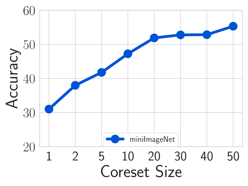
Figure 9: How much inference memory? Enlarging the coreset size of the VRF kernel leads to improvement of performance on miniImageNet benchmark dataset. Coreset size 30 is chosen for conducting experiment in the main paper.

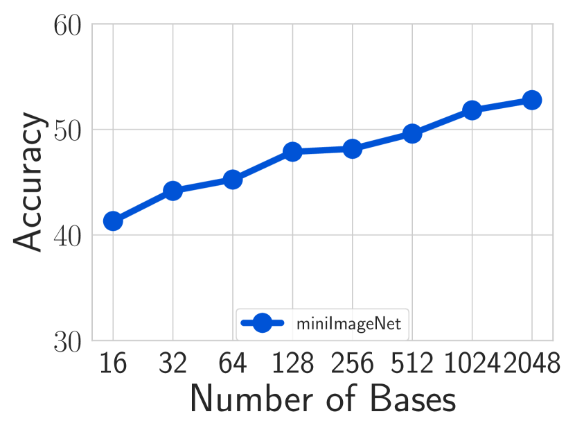
Figure 10: How many Random Bases? In general, a larger number of random Fourier bases consistently improves performance on miniImageNet benchmark dataset. In the main paper, number of bases is set to be 2048.

References

- Aljundi et al. (2018) Aljundi, R., Babiloni, F., Elhoseiny, M., Rohrbach, M., and Tuytelaars, T. Memory aware synapses: Learning what (not) to forget. In European Conference on Computer Vision, 2018.
- Bach et al. (2004) Bach, F. R., Lanckriet, G. R., and Jordan, M. I. Multiple kernel learning, conic duality, and the SMO algorithm. In International Conference on Machine Learning, 2004.
- Carratino et al. (2018) Carratino, L., Rudi, A., and Rosasco, L. Learning with sgd and random features. In Advances in Neural Information Processing Systems, 2018.
- Chaudhry et al. (2018) Chaudhry, A., Dokania, P. K., Ajanthan, T., and Torr, P. H. S. Riemannian walk for incremental learning: Understanding forgetting and intransigence. In European Conference on Computer Vision, 2018.
- Chaudhry et al. (2019a) Chaudhry, A., Ranzato, M., Rohrbach, M., and Elhoseiny, M. Efficient lifelong learning with A-GEM. In International Conference on Learning Representations, 2019a.
- Chaudhry et al. (2019b) Chaudhry, A., Rohrbach, M., Elhoseiny, M., Ajanthan, T., Dokania, P. K., Torr, P. H. S., and Ranzato, M. On tiny episodic memories in continual learning. In Advances in Neural Information Processing Systems, 2019b.
- Chaudhry et al. (2020) Chaudhry, A., Khan, N., Dokania, P. K., and Torr, P. H. Continual learning in low-rank orthogonal subspaces. In Advances in Neural Information Processing System, 2020.
- Cristianini et al. (2000) Cristianini, N., Shawe-Taylor, J., et al. An introduction to support vector machines and other kernel-based learning methods. Cambridge university press, 2000.
- Diehl & Cauwenberghs (2003) Diehl, C. P. and Cauwenberghs, G. Svm incremental learning, adaptation and optimization. In Proceedings of the International Joint Conference on Neural Networks, 2003.
- Ebrahimi et al. (2020) Ebrahimi, S., Elhoseiny, M., Darrell, T., and Rohrbach, M. Uncertainty-guided continual learning with bayesian neural networks. In International Conference on Learning Representations, 2020.
- Goodfellow et al. (2014) Goodfellow, I. J., Mirza, M., Xiao, D., Courville, A., and Bengio, Y. An empirical investigation of catastrophic forgeting in gradientbased neural networks. In International Conference on Learning Representations, 2014.
- Gordon et al. (2019) Gordon, J., Bronskill, J., Bauer, M., Nowozin, S., and Turner, R. E. Meta-learning probabilistic inference for prediction. In International Conference on Learning Representations, 2019.
- Hadsell et al. (2020) Hadsell, R., Rao, D., Rusu, A. A., and Pascanu, R. Embracing change: Continual learning in deep neural networks. Trends in Cognitive Sciences, 2020.
- Jerfel et al. (2019) Jerfel, G., Grant, E., Griffiths, T. L., and Heller, K. A. Reconciling meta-learning and continual learning with online mixtures of tasks. In Advances in Neural Information Processing Systems, 2019.
- Kingma & Welling (2014) Kingma, D. P. and Welling, M. Auto-encoding variational bayes. In International Conference on Learning Representations, 2014.
- Kirkpatrick et al. (2017) Kirkpatrick, J., Pascanu, R., Rabinowitz, N., Veness, J., Desjardins, G., Rusu, A. A., Milan, K., Quan, J., Ramalho, T., Grabska-Barwinska, A., Hassabis, D., Clopath, C., Kumaran, D., and Hadsell, R. Overcoming catastrophic forgetting in neural networks. Proceedings of the National Academy of Sciences, 114(13):3521–3526, 2017.
- Kolouri et al. (2019) Kolouri, S., Ketz, N., Zou, X., Krichmar, J., and Pilly, P. Attention-based structural-plasticity. arXiv preprint arXiv:1903.06070, 2019.
- Lange et al. (2019) Lange, M., Aljundi, R., Masana, M., Parisot, S., Jia, X., Leonardis, A., Slabaugh, G. G., and Tuytelaars, T. Continual learning: A comparative study on how to defy forgetting in classification tasks. arXiv preprint arXiv:1909.08383, 2019.
- LeCun et al. (2015) LeCun, Y., Bengio, Y., and Hinton, G. Deep learning. Nature, 2015.
- Lee et al. (2017) Lee, S.-W., Kim, J.-H., Jun, J., Ha, J.-W., and Zhang, B.-T. Overcoming catastrophic forgetting by incremental moment matching. In Advances in Neural Information Processing Systems, 2017.
- Li et al. (2019) Li, X., Zhou, Y., Wu, T., Socher, R., and Xiong, C. Learn to grow: A continual structure learning framework for overcoming catastrophic forgetting. In International Conference on Machine Learning, 2019.
- Lopez-Paz & Ranzato (2017) Lopez-Paz, D. and Ranzato, M. Gradient episodic memory for continual learning. In Advances in Neural Information Processing Systems, 2017.
- Mallya & Lazebnik (2018) Mallya, A. and Lazebnik, S. Packnet: Adding multiple tasks to a single network by iterative pruning. In IEEE Conference on Computer Vision and Pattern Recognition, 2018.
- Masse et al. (2018) Masse, N. Y., Grant, G. D., and Freedman, D. J. Alleviating catastrophic forgetting using context-dependent gating and synaptic stabilization. Proceedings of the National Academy of Sciences, 115(44), 2018.
- McCloskey & Cohen (1989) McCloskey, M. and Cohen, N. J. Catastrophic interference in connectionist networks: The sequential learning problem. Academic Press, 1989.
- Mirzadeh et al. (2020) Mirzadeh, S. I., Farajtabar, M., Pascanu, R., and Ghasemzadeh, H. Understanding the role of training regimes in continual learning. In Advances in Neural Information Processing Systems, 2020.
- Nguyen et al. (2018) Nguyen, C. V., Li, Y., Bui, T. D., and Turner, R. E. Variational continual learning. In International Conference on Learning Representations, 2018.
- Parisi et al. (2018) Parisi, G., Kemker, R., Part, J. L., Kanan, C., and Wermter, S. Continual lifelong learning with neural networks: A review. Neural Networks, 2018.
- Paszke et al. (2019) Paszke, A., Gross, S., Massa, F., and et. al. Pytorch: An imperative style, high-performance deep learning library. 2019.
- Patacchiola et al. (2020) Patacchiola, M., Turner, J., Crowley, E. J., O’Boyle, M., and Storkey, A. Bayesian meta-learning for the few-shot setting via deep kernels. In Advances in Neural Information Processing Systems, 2020.
- Pentina & Ben-David (2015) Pentina, A. and Ben-David, S. Multi-task and lifelong learning of kernels. In International Conference on Algorithmic Learning Theory, 2015.
- Rahimi & Recht (2007) Rahimi, A. and Recht, B. Random features for large-scale kernel machines. In Advances in Neural Information Processing Systems, 2007.
- Ramasesh et al. (2021) Ramasesh, V. V., Dyer, E., and Raghu, M. Anatomy of catastrophic forgetting: Hidden representations and task semantics. International Conference on Learning Representations, 2021.
- Rebuffi et al. (2017) Rebuffi, S.-A., Kolesnikov, A. I., Sperl, G., and Lampert, C. H. iCaRL: Incremental classifier and representation learning. In IEEE Conference on Computer Vision and Pattern Recognition, 2017.
- Riemer et al. (2019) Riemer, M., Cases, I., Ajemian, R., Liu, M., Rish, I., Tu, Y., and Tesauro, G. Learning to learn without forgetting by maximizing transfer and minimizing interference. In International Conference on Learning Representations, 2019.
- Ring (1998) Ring, M. B. Child: A first step towards continual learning. Learning to learn, 1998.
- Rios & Itti (2018) Rios, A. and Itti, L. Closed-loop gan for continual learning. In International Joint Conference on Artificial Intelligence, 2018.
- Ritter et al. (2018) Ritter, H., Botev, A., and Barber, D. Online structured laplace approximations for overcoming catastrophic forgetting. In Advances in Neural Information Processing Systems, 2018.
- Rudin (1962) Rudin, W. Fourier analysis on groups. Wiley Online Library, 1962.
- Russakovsky et al. (2015) Russakovsky, O., Deng, J., Su, H., Krause, J., Satheesh, S., Ma, S., Huang, Z., Karpathy, A., Khosla, A., Bernstein, M., et al. Imagenet large scale visual recognition challenge. International journal of computer vision, 2015.
- Rusu et al. (2016) Rusu, A. A., Rabinowitz, N. C., Desjardins, G., Soyer, H., Kirkpatrick, J., Kavukcuoglu, K., Pascanu, R., and Hadsell, R. Progressive neural networks. In Advances in Neural Information Processing Systems, 2016.
- Schmidhuber (2015) Schmidhuber, J. Deep learning in neural networks: An overview. Neural Networks, 2015.
- Schölkopf & Smola (2002) Schölkopf, B. and Smola, A. J. Learning with kernels. MIT Press, 2002.
- Schölkopf et al. (2001) Schölkopf, B., Herbrich, R., and Smola, A. J. A generalized representer theorem. In International Conference on Computational Learning Theory, 2001.
- Schwarz et al. (2018) Schwarz, J., Czarnecki, W., Luketina, J., Grabska-Barwinska, A., Teh, Y. W., Pascanu, R., and Hadsell, R. Progress & compress: A scalable framework for continual learning. In International Conference on Machine Learning, 2018.
- Shin et al. (2017) Shin, H., Lee, J. K., Kim, J., and Kim, J. Continual learning with deep generative replay. In Advances in Neural Information Processing Systems, 2017.
- Sinha & Duchi (2016) Sinha, A. and Duchi, J. C. Learning kernels with random features. In Advances in Neural Information Processing Systems, 2016.
- Smola & Schölkopf (2004) Smola, A. J. and Schölkopf, B. A tutorial on support vector regression. Statistics and computing, 2004.
- Titsias et al. (2020) Titsias, M. K., Schwarz, J., Matthews, A. G. d. G., Pascanu, R., and Teh, Y. W. Functional regularisation for continual learning using gaussian processes. In International Conference on Learning Representations, 2020.
- Tossou et al. (2019) Tossou, P., Dura, B., Laviolette, F., Marchand, M., and Lacoste, A. Adaptive deep kernel learning. In Advances in Neural Information Processing Systems, 2019.
- Vinyals et al. (2016) Vinyals, O., Blundell, C., Lillicrap, T., Kavukcuoglu, K., and Wierstra, D. Matching networks for one shot learning. In Advances in Neural Information Processing Systems, 2016.
- Wilson et al. (2016a) Wilson, A. G., Hu, Z., Salakhutdinov, R., and Xing, E. P. Deep kernel learning. In International Conference on Artificial Intelligence and Statistics, 2016a.
- Wilson et al. (2016b) Wilson, A. G., Hu, Z., Salakhutdinov, R., and Xing, E. P. Stochastic variational deep kernel learning. In Advances in Neural Information Processing Systems, 2016b.
- Wortsman et al. (2020) Wortsman, M., Ramanujan, V., Liu, R., Kembhavi, A., Rastegari, M., Yosinski, J., and Farhadi, A. Supermasks in superposition. In Advances in Neural Information Processing Systems, 2020.
- Yoon et al. (2018) Yoon, J., Yang, E., Lee, J., and Hwang, S. J. Lifelong learning with dynamically expandable networks. In International Conference on Learning Representations, 2018.
- Zenke et al. (2017) Zenke, F., Poole, B., and Ganguli, S. Continual learning through synaptic intelligence. In International Conference on Machine Learning, 2017.
- Zhang et al. (2019) Zhang, M., Wang, T., Lim, J. H., and Feng, J. Prototype reminding for continual learning. arXiv preprint arXiv:1905.09447, 2019.
- Zhen et al. (2020) Zhen, X., Sun, H., Du, Y., Xu, J., Yin, Y., Shao, L., and Snoek, C. Learning to learn kernels with variational random features. In International Conference on Machine Learning, 2020.