Which Molecular Cloud Structures Are Bound?

Abstract

We analyze surveys of molecular cloud structures defined by tracers ranging from CO $J=1\rightarrow 0$ through ¹³CO $J=1\rightarrow 0$ to dust emission together with NH₃ data. The mean value of the virial parameter and the fraction of mass in bound structures depends on the method used to identify structures. Generally, the virial parameter decreases and the fraction of mass in bound structures increases with the effective density of the tracer, the surface density and mass of the structures, and the distance from the center of a galaxy. For the most complete surveys of structures defined by CO $J=1\rightarrow 0$, the fraction of mass that is in bound structures is 0.19. substantial alleviation of the fundamental problem of slow star formation. If only clouds found to be bound are counted and they are assumed to collapse in a free-fall time at their mean cloud density, the sum over all clouds in a complete survey of the Galaxy yields a predicted star formation rate of 46 M_⊙ yr^-1, a factor of 6.5 less than if all clouds are bound.

1 Introduction

The fundamental problem of star formation was first stated by Zuckerman & Palmer (1974) and Zuckerman & Evans (1974). Simply stated, a theoretical estimate of the star formation rate in the Milky Way exceeded by a factor of about 100 the rate averaged over the last Gyr or so, as inferred from observations. Those early estimates were based on preliminary surveys of the Galaxy in CO and estimates of the average star formation rate, but the situation has only worsened after nearly a half century of improved surveys. Heyer & Dame (2015) estimated a mass of $(1.0\pm 0.3)\times 10^{9}$ M_⊙ for the total molecular gas in the Galaxy. The free-fall time,

$$\mbox{$t_{\rm ff}$}=\bigg{(}\frac{3\pi}{32G\rho}\bigg{)}^{0.5}=3.34\mbox{${}\times 10^{7}$}n^{-0.5}{\rm yr}=\\ 1.66\mbox{${}\times 10^{7}$}r_{\rm pc}^{1.5}M_{\mbox{M${}_{\odot}$}}^{-0.5}{\rm yr},$$ (1)

where $n$ is the particle density , related to $\rho$ by the mean mass per particle of 2.37 (Kauffmann et al. 2008). For a characteristic density of 100 cm^-3, $\mbox{$t_{\rm ff}$}=3.34\mbox{${}\times 10^{6}$}$ yr, predicting a star formation rate of 300 M_⊙ yr^-1. In contrast, observational data indicate much lower rates. Counting young stars from the GLIMPSE (Benjamin et al. 2003; Churchwell et al. 2009) survey, Robitaille & Whitney (2010) constrained the star formation rate to 0.68-1.45 M_⊙ yr^-1, averaged over the lifetime of infrared excesses around young stars, roughly the last few Myr. Using a wider range of indicators, Chomiuk & Povich (2011) derived a star formation rate of $1.9\pm 0.4$ M_⊙ yr^-1, which we adopt. The discrepancy has, if anything, worsened with further research to a factor of 160.

This problem arises because the molecular clouds identified by CO emission are assumed to be gravitationally bound and collapsing on a free-fall timescale. This problem is properly called the slowness of star formation (Krumholz et al. 2014; Padoan et al. 2014) and parameterized by the efficiency per free-fall time, $\epsilon_{\rm ff}$. which is taken to be 0.01, reflecting the factor of 100 problem identified by the first references, but the latest numbers suggest $\mbox{$\epsilon_{\rm ff}$}=0.006$. Another expression of the slowness is that the depletion time, given by the molecular mass divided by the star formation rate, is $\mbox{$t_{\rm dep}$}=5\mbox{${}\times 10^{8}$}$ yr, much larger than $t_{\rm ff}$. The depletion time is even longer in other galaxies, $\mbox{$t_{\rm dep}$}\approx 2$ Gyr (Bigiel et al. 2008).

A somewhat distinct problem is the final efficiency of star formation, $\epsilon_{\rm sf}$, defined by

$${\mbox{$\epsilon_{\rm sf}$}=M_{*}/M_{\rm gas},}$$ (2)

where $M_{*}$ is the mass in stars at the end of the event and $M_{\rm gas}$ is the mass of gas at the beginning. While we cannot measure these for an individual cloud, star clusters that have formed reasonably recently (i.e., leaving aside globular clusters) are much less massive than the mass in clouds. We can compare the mass function of molecular clouds to that of clusters. The mass functions, expressed per logarithmic unit of mass are expressed as

$$\frac{dN}{d\log M}\propto(M/M_{\rm u,x})^{\Gamma_{\rm x}}$$ (3)

where $M$ is the mass of entity $x$, up to a maximum mass $M_{\rm u,x}$. For Milky Way OB assocations and clusters, $\Gamma_{\rm cluster}$ is $-1.0$ and $M_{\rm u,cluster}$ is about 6${}\times 10^{4}$ M_⊙ (Massey et al. 1995; McKee & Williams 1997; Portegies Zwart et al. 2010). For molecular clouds, the values are $\Gamma_{\rm cloud}=-0.6$ and $M_{\rm u,cloud}=6\mbox{${}\times 10^{6}$}$ M_⊙ (Williams & McKee 1997). See also Rosolowsky (2005), who give results in terms of $\gamma=\Gamma_{\rm cloud}+1$, with our definition of $\Gamma_{\rm cloud}$. The ratio of upper mass limits suggests that $\mbox{$\epsilon_{\rm sf}$}=0.01$, but the differences in the slopes suggests that molecular clouds are not the immediate precursors of clusters and associations. Dense clumps, in contrast, have a similar slope and upper mass limit to those of clusters and associations. Shirley et al. (2003) found $\Gamma_{\rm clump}=-1.0$ for dense clumps defined by strong CS $J=5\rightarrow 4$ emission. Elia et al. (2017) found $\Gamma_{\rm clump}=-1.05\pm 0.08$ in a sample of $10^{4}$ clumps defined from submillimeter continuum emission. The upper mass limit for clumps, $M_{\rm u,clump}$ is about 1${}\times 10^{5}$ M_⊙ based on various studies (Shirley et al. 2003; Svoboda et al. 2016; Urquhart et al. 2018).

Much theoretical ingenuity has been expended to solve the problem of slow star formation. Magnetic fields may help to “support” clouds, and turbulence can slow collapse. However, numerical simulations generally found that supersonic turbulence should decay rapidly, with or without magnetic fields (Stone et al. 1998; Mac Low 1999). Also, turbulence appears to be driven on scales larger than the cloud, rather than from within the cloud (Larson 1981; Heyer & Brunt 2004; Brunt et al. 2009).

The kind of solution that invokes turbulence to support a cloud has the problem of the inherent instability of a gravitationally bound entity. It is hard to imagine an individual cloud avoiding gravitational collapse for a depletion time that is over 200 times the free-fall time. Indeed, Heyer & Dame (2015) placed a strong upper limit on cloud lifetime ($t_{\rm cloud}$) of $10^{8}$ yr and preferred a lifetime of $3\mbox{${}\times 10^{7}$}$ yr, based on Kawamura et al. (2009), closer to 10 times the canonical value for $t_{\rm ff}$. Clearly most of the mass in clouds must disperse after a star forming event. The low value of $\epsilon_{\rm sf}$ suggests that 99.4% is dispersed. Another approach has been to question the use of the current density to estimate the free-fall time (Vázquez-Semadeni et al. 2019). A lower initial density would slow the initial rate of collapse, but the conflict with the prediction based on current properties of molecular clouds remains.

Recent theoretical work has concentrated on feedback to remove most of the gas before it forms stars For example, Kim et al. (2018) compared the effectiveness of radiation pressure and photoionization in disrupting clouds. Even though they started with marginally bound clouds, the final efficiencies, $\epsilon_{\rm sf}$, increased strongly with increasing initial cloud surface density ($\Sigma_{\rm M}$), exceeding 5% by initial $\mbox{$\Sigma_{\rm M}$}=20$ M_⊙ pc^-2 (figure 7 of their paper). Bound clouds overproduce stars even at very low initial $\Sigma_{\rm M}$, even with strong radiative feedback. Another interesting feature of figure 7 of Kim et al. (2018) is that $\epsilon_{\rm sf}$ reaches about 0.5 at $\mbox{$\Sigma_{\rm M}$}\sim\mbox{$10^{3}$}$ M_⊙ pc^-2, similar to the surface density of the dense clumps studied by Shirley et al. (2003). If these were the bound entities, the ratio of maximum cluster mass to initial gas mass would come out about right. Simulations of unbound clouds look more promising. Kim et al. (2021) have performed radiative magnetohydrodynamical simulations (RMHD) for clouds with starting $\mbox{$\Sigma_{\rm M}$}=80$ M_⊙ pc^-2, reasonably appropriate to the structures traced by CO. The star formation is limited by feedback from massive stars. They found that both $\epsilon_{\rm ff}$ and $\epsilon_{\rm sf}$ decrease with increasing virial parameter ($\alpha_{\rm vir,0}$), reaching values similar to the observed values for $\mbox{$\alpha_{\rm vir,0}$}\sim 5$.

In the current situation, it seems prudent to reexamine the assumptions underlying the fundamental problem: that all molecular clouds are gravitationally bound and that they are collapsing at free-fall, with the free-fall time calculated from the mean cloud density of 100 cm^-3. The question of whether the cloud is bound is usually addressed by calculating the virial parameter, $\alpha_{\rm vir}$ (Bertoldi & McKee 1992). The definition of this parameter varies. The most common definition assumes virial equilibrium. Ignoring surface terms and magnetic fields,

$$\mbox{$\alpha_{\rm vir}$}=\frac{2E_{kin}}{|E_{g}|},$$ (4)

where $E_{g}$ is the gravitational potential energy and $E_{kin}$ is the kinetic energy. With this definition, the dividing line between bound and unbound is $\mbox{$\alpha_{\rm vir}$}=2$, where $E_{kin}=|E_{g}|$. Surface pressure from the surrounding medium would increase $\alpha_{\rm vir}$ while magnetic fields would decrease $\alpha_{\rm vir}$ (Tan et al. 2013). Because we cannot measure them, we neglect the largely unknown pressure and magnetic terms. Then a cloud with $E_{kin}>E_{g}$ would tend to expand or dissipate, so we take $\mbox{$\alpha_{\rm vir}$}=2$ as our critical value to define a cloud as bound if $\mbox{$\alpha_{\rm vir}$}<2$ and unbound if $\mbox{$\alpha_{\rm vir}$}>2$.

The calculation of $E_{g}$ depends on cloud shape and structure (Bertoldi & McKee 1992; Kauffmann et al. 2013) but these effects can be considered as correction factors for the expression for a uniform density sphere:

$$E_{g}=\frac{-3GM^{2}}{5R}.$$ (5)

where M and R are the cloud mass and radius. The kinetic energy is estimated from

$$E_{kin}=\frac{3\mbox{$\sigma_{v}$}^{2}M}{2}$$ (6)

where $\sigma_{v}$ is the one-dimensional velocity dispersion averaged over the cloud.

Unbound clouds may of course contain bound structures. Measuring $\alpha_{\rm vir}$ in the complex structures of the ISM is more problematic, as surface terms are likely to be important (Mao et al. 2020). Kim et al. (2021) compared the virial parameters from their model clouds to those that would be derived from observations. They found that the methods used by observers are more likely to overestimate the boundedness of the cloud, but generally by factors of 2 or less. They caution that neglect of tidal effects in crowded regions would make the overestimation worse. This effect was indeed apparent in larger-scale simulations (Mao et al. 2020), which found that many regions that were apparently bound, based on the criteria that $\mbox{$\alpha_{\rm vir}$}<2$ were in fact unbound. In particular, the boundedness of large massive structures was more likely to be overestimated using the simpler estimations available to observers.

Given our simple approach to the virial parameter, ignoring external pressure, magnetic fields, and tides, we use the term “bound” as shorthand for gravitationally bound. A cloud could be unbound in our definition, but contained or “bound” by external pressure. Our focus is on whether gravity or turbulence is dominant. If the results of the simulations discussed above apply, our criteria for boundedness will be more generous than reality. We calculate virial parameters from

$$\mbox{$\alpha_{\rm vir}$}=\frac{2E_{kin}}{|E_{g}|}=1160\mbox{$\sigma_{v}$}^{2}R_{pc}/M_{\mbox{M${}_{\odot}$}}=\\ 209\mbox{$\Delta v$}^{2}R_{pc}/M_{\mbox{M${}_{\odot}$}},$$ (7)

where $M_{\mbox{M${}_{\odot}$}}$ is the actual mass of the cloud in solar masses.

Estimating the actual mass of the cloud can be done in a number of ways, but the original source of the fundamental problem relied on observations of the lowest rotational transition of CO. The problem is that this line is usually very optically thick. Many words have been expended explaining why this can work, including an implicit assumption that the clouds are in virial equilibrium (e.g., Bolatto et al. 2013). If this were the only argument, the whole discussion would be circular, but we will take the CO-derived masses as independent of the assumption of virial equilibrium. The correlation of CO emission with dust extinction via the $X({\rm CO})$ factor provides an independent basis for its use in determining column density (Dickman 1978; Pineda et al. 2010; Heiderman et al. 2010). While column density may be underestimated at high column density and overestimated at low column density, both by factors of 2 or more, Bolatto et al. (2013) argued that variations in $X$(CO) average out, so $L$(CO) may reflect mass better than the intensity traces column density for a particular line of sight. The relation is $\mbox{$M_{\rm CO}$}=\mbox{$\alpha_{\rm CO}$}\mbox{$L_{\rm CO}$}$. We follow Bolatto et al. (2013) in taking $\alpha_{\rm CO}$ of 4.3 M_⊙(K km s^-1 pc²)^-1.

Samples using ¹³CO $J=1\rightarrow 0$ to get mass usually combine the ¹³CO data with CO data to derive the optical depth and then column density of ¹³CO, $N_{\rm 13}$, assuming that the excitation temperatures of CO and ¹³CO are equal and that the partition function can be approximated by assuming that the excitation temperature applies to all levels (commonly referred to as the “LTE” assumption). The excitation temperature can be found from the CO brightness temperature. Because we use CO data with low spatial resolution, we instead assume an excitation temperature of 8 K for all lines of sight (Roman-Duval et al. 2010). We follow the description by Ripple et al. (2013) but note the error in their equation 4, in which the exponential factor should be in the denominator. Conversion to the column density of H₂ follows

$$N({\rm H_{2}})=N_{\rm 13}\Bigl{[}\frac{{\rm H_{2}}}{\rm CO}\Bigr{]}\Bigl{[}\frac{\rm CO}{\mbox{${}^{13}$CO}}\Bigr{]}.$$ (8)

We have used the latest number for H₂/CO of 6000 (Lacy et al. 2017). Because the new measurement directly relates the abundance of H₂, not including helium, to that of CO through infrared absorption observations, we use the mean molecular weight of $\mbox{$\mu_{\rm H_{2}}$}m_{\rm H}$, with $\mbox{$\mu_{\rm H_{2}}$}=2.8$ to convert to mass (Kauffmann et al. 2008). We have corrected data to use these values. Unless otherwise noted, when analyzing the ¹³CO $J=1\rightarrow 0$ data, we account for a Galactic gradient in ${\rm CO}/{\rm{}^{13}CO}$. We apply the elemental isotope gradient in the Galaxy most recently derived by Jacob et al. (2020),

$$\frac{{}^{12}{\rm C}}{{}^{13}{\rm C}}=5.87\mbox{$R_{\rm gal}$}+13.25,$$ (9)

where $R_{\rm gal}$ is the distance of the cloud from the Galactic Center in kpc.

2 Samples

The sets of data used in this paper are listed in Table 1. We consider structures defined by CO emission, ¹³CO emission, and dust emission, supplemented by molecular line data. From the catalogs in the papers, we extracted the information on size, mass, mass surface density ($\Sigma_{\rm M}$) and virial parameter ($\alpha_{\rm vir}$), or the parameters needed to calculate them. In most cases, some pruning of the catalog entries was necessary. The cuts used are explained below.

2.1 Structures Defined by CO $J=1\rightarrow 0$ Emission

The samples in this category rely on masses measured from the luminosity of the $J=1\rightarrow 0$ transition of CO. The conversion from luminosity to mass ($\alpha_{\rm CO}$) differed somewhat among the studies; to standardize them, the value of $M_{\rm CO}$ in the Milky Way samples was calculated using $\mbox{$\alpha_{\rm CO}$}=4.3$ M_⊙(K km s^-1 pc²)^-1 (Bolatto et al. 2013).

Table 1: Sample List

Name	Tracer	Reference	Notes
CO-Rice	CO $J=1\rightarrow 0$	Rice et al. (2016)	1
CO-MD	CO $J=1\rightarrow 0$	Miville-Deschênes et al. (2017)	2
CO-CMZ	CO $J=1\rightarrow 0$	Oka et al. (2001)	3
CO-OGS	CO $J=1\rightarrow 0$	Heyer et al. (2001)	4
CO-Sun	CO $J=1\rightarrow 0$	Sun et al. (2020)	5
13CO-GRS	13CO $J=1\rightarrow 0$	Roman-Duval et al. (2010)	6
13CO-EXFC55-100	13CO $J=1\rightarrow 0$	Roman-Duval et al. (2016)	7
13CO-EXFC135-195	13CO $J=1\rightarrow 0$	Roman-Duval et al. (2016)	8
13CO-SEDIGISM	13CO $J=2\rightarrow 1$	Duarte-Cabral et al. (2021)	9
Herschel	submillimeter$+$ NH3	Merello et al. (2019)	10

Notes: 1. Recovers 25% of emission in the survey by Dame et al. (2001).
2. Recovers 98% of emission in the survey by Dame et al. (2001).
3. Attempted to restrict to CMZ.
4. Outer Galaxy Survey: $\mbox{$\langle\mbox{$R_{\rm gal}$}\rangle$}=11.8\pm 1.3$
5. Survey of 66 galaxies.
6. Galactic Ring Survey: $\mbox{$\langle\mbox{$R_{\rm gal}$}\rangle$}=5.2\pm 1.0$
7. Exeter-FCRAO Survey for $55<l<100$: $\mbox{$\langle\mbox{$R_{\rm gal}$}\rangle$}=10.3\pm 1.9$
8. Exeter-FCRAO Survey for $135<l<195$: $\mbox{$\langle\mbox{$R_{\rm gal}$}\rangle$}=12.9\pm 2.1$
9. Covers $R_{\rm gal}$ from 0.6 to 15.7 kpc: $\mbox{$\langle\mbox{$R_{\rm gal}$}\rangle$}=5.5\pm 1.8$
10. Based on the Herschel Infrared Galactic Plane Survey

New catalogs of clouds based on decomposition of the CO surveys are now available (Rice et al. 2016; Miville-Deschênes et al. 2017). These are particularly interesting as they used the data from Dame et al. (2001) that was featured by Heyer & Dame (2015) but analyzed it in two different ways. These two studies, labeled CO-Rice and CO-MD in Table 1, take different approaches to breaking the large scale CO emission in the Galaxy into clouds, and we will discuss the effect of those differences in §4.1.

Rice et al. (2016) used a dendrogram analysis to identify 1064 clouds. They recovered 2.5${}\times 10^{8}$ M_⊙, about 25% of the total molecular mass of the Galaxy. Table 3 of Rice et al. (2016) provides a radius, $\sigma_{v}$, and $M_{\rm CO}$, the mass determined from the CO luminosity, which we use directly. The mass surface density was determined from $M_{\rm CO}$ and the radius. No mass or size information was given for clouds without clear resolution of the kinematic distance ambiguity, and one cloud was assigned zero size and mass in Table 3 of Rice et al. (2016); after removing these, 1037 clouds remained for our analysis.

Miville-Deschênes et al. (2017) used a Gaussian decomposition and hierarchical cluster analysis to assign essentially all the CO emission in the Dame survey to 8107 clouds comprising $1.2\mbox{${}\times 10^{9}$}$ M_⊙. Their online table provides radii and masses for both near and far kinematic distances, along with a code for resolution of the kinematic distance ambiguity, which we use to select the best radius and mass. Miville-Deschênes et al. (2017) calculated a radius from the two projected radii by $r=(r_{\rm max}r_{\rm min}r_{\rm min})^{1/3}$, arguing that the depth was more likely equal to the smaller size projected on the sky. They also provide $\sigma_{v}$, which we use in calculating $\alpha_{\rm vir}$. The masses were based on summing column densities, using $X_{\rm CO}=2\mbox{${}\times 10^{20}$}$ cm^-2 (K km s^-1)^-1, which corresponds to $\mbox{$\alpha_{\rm CO}$}=4.3$ M_⊙(K km s^-1 pc²)^-1 (Bolatto et al. 2013). The catalog contains a small number of clouds with nominal Galactocentric radii greater than 30 kpc and a large number of low-mass objects with very high $\alpha_{\rm vir}$. To select against these, we require that $R_{\rm gal}<30$ kpc, $\mbox{$M_{\rm CO}$}>1$ M_⊙ and $\mbox{$\alpha_{\rm vir}$}<\mbox{$\alpha_{\rm max}$}$, where $\alpha_{\rm max}$ is an arbitrarily chosen maximum value. Entry 2 in Table 2 required $\mbox{$\alpha_{\rm vir}$}<100$, while entry 3 used $\mbox{$\alpha_{\rm vir}$}<20$.

The sample labeled CO-CMZ in Table 1 is from Oka et al. (2001) and focuses on clouds in the Central Molecular Zone (CMZ) using data obtained with the Nobeyama Radio Observatory 45-m telescope. Clouds were defined by topologically closed surfaces in $(l,b,v)$ space. Three different thresholds were used and some clouds appear multiple times in the catalog, providing a range of surface densities. The dispersions in all three coordinates were used to define sizes and linewidths. A distance of 8.5 kpc was used for all clouds. They accounted for truncation by the threshold by comparing to simulated clouds and provided corrected values for sizes, velocity dispersions, and CO luminosities. These are what we use. To calculate the mass surface density, we take the size as a radius. They also computed virial masses, but we do not use these. We eliminate clouds determined to be outside the CMZ (labeled D in their table 1) or confused (labeled with C in their table 1). The use of $\mbox{$\alpha_{\rm CO}$}=4.3$ M_⊙(K km s^-1 pc²)^-1 in the CMZ is dubious. Oka et al. (1998) suggested a value 10 times smaller. Elemental abundances certainly are higher in the CMZ and a correction for that might be appropriate, as suggested by Sun et al. (2020) for other galaxies.

The sample labeled CO-OGS in Table 1 is a sample of clouds in the outer Galaxy mapped by the FCRAO 14-m telescope (Heyer et al. 1998) and tabulated by Heyer et al. (2001). The Table provides $L_{\rm CO}$, $\Delta v$ (FWHM), and diameter of the structure. Heyer et al. (2001) used $\mbox{$\alpha_{\rm CO}$}=4.1$ to convert to mass, but we changed to 4.3 for consistency. We convert diameter to radius for consistency. The linewidth used to calculate $M_{\rm vir}$ was that of a spectrum averaged over the cloud. These were almost always larger than an alternative estimate using the dispersion of line centroids over the cloud, indicating that the clouds are generally not dominated by systematic motions such as shear. The catalog contains 10156 structures, but many are local. To select outer Galaxy sources, Heyer et al. (2001) required $\mbox{$v_{LSR}$}<-25$ km s^-1. To select against small structures, they also required $\mbox{$M_{\rm CO}$}>2.5\mbox{${}\times 10^{3}$}$ M_⊙. We give values for this cut, but we relax it to $\mbox{$M_{\rm CO}$}>10$ M_⊙ for the figures and most analysis because we are more interested in completeness in structures than in defining a mass function.

2.2 Structures Defined by CO $J=2\rightarrow 1$ Emission in Other Galaxies

Studies of other galaxies are beginning to provide similar information without the line-of-sight confusion of Milky Way studies. For other galaxies, we use the remarkable compilation by Sun et al. (2020) of the PHANGS-ALMA study of the CO $J=2\rightarrow 1$ transition, labeled CO-Sun in Table 1, which is part of a larger program including HST observations (Lee et al. 2021). They collected data on over $10^{5}$ sightlines toward 66 galaxies, resampled to a uniform spatial resolution of 150 pc, by far the largest data base available, albeit with very poor spatial resolution by the standards of studies in our Galaxy. They used a metallicity dependent value for $\alpha_{\rm CO}$, and we use their values. Their table 2 provides $\Sigma_{\rm M}$ and $\alpha_{\rm vir}$. We compute $M_{\rm CO}$ from $\Sigma_{\rm M}$ and the fixed size of 150 pc and use their $\alpha_{\rm vir}$.

2.3 Structures Defined by ¹³CO $J=1\rightarrow 0$ Emission

Roman-Duval et al. (2010) provided the sample defined by ¹³CO $J=1\rightarrow 0$ emission from the Galactic Ring Survey (GRS) by Jackson et al. (2006). The ¹³CO data were combined with the CO data from the University of Massachusetts-Stony Brook (UMSB) survey (Sanders et al. 1985; Clemens et al. 1986) to determine optical depth and ¹³CO column density. The clouds in the Roman-Duval et al. (2010) study were actually identified by Rathborne et al. (2009), who presented a detailed description of the method, using CLUMPFIND (Williams et al. 1994) and a number of tests to be able to identify both bright, compact structures and fainter, more diffuse structures. The effective lowest brightness level was 0.2 K, so they should not have selected regions of abnormally high density.

For the original analysis by Roman-Duval et al. (2010) of the GRS survey, we consider these to be structures defined by ¹³CO. Radius, mass, surface density, and $\alpha_{\rm vir}$ are provided by their table 1, with 749 entries. Requiring $\mbox{$M_{\rm CO}$}>1$ M_⊙, $\mbox{$\Sigma_{\rm M}$}>10$ M_⊙ pc^-2, and $\mbox{$\alpha_{\rm vir}$}<20$ pruned the sample to 737. The condition on $\alpha_{\rm vir}$ removed a few extreme outliers. 170 clouds in the sample were not covered by the UMSB CO survey, so the usual method to determine the column density of ¹³CO was impractical. If we exclude those, the results do not differ substantially. Roman-Duval et al. (2010) used a different definition of $\alpha_{\rm vir}$, assuming a correction for the density distribution. For consistency, we recalculated $\alpha_{\rm vir}$ from Equation 7. These values were larger by a factor of 1.3 on average than those given in their paper when the same assumptions about abundances were made.

For the ¹³CO $J=1\rightarrow 0$ samples from other parts of the Galaxy, both ¹³CO and CO $J=1\rightarrow 0$ were observed simultaneously. These are the Exeter-FCRAO surveys, which are divided into EXFC55-100 and EXFC135-195, but our analysis excludes the range of longitude where kinematic distances are unreliable ($165<l<195$), as described by Roman-Duval et al. (2016). For the EXFC surveys, Roman-Duval et al. (2016) attempted to identify all voxels with emission to distinguish diffuse (CO only) from “dense” gas (¹³CO and CO). Structures were not identified and no catalogs were provided. We have re-analyzed all the ¹³CO $J=1\rightarrow 0$ surveys in a uniform way, using the CO-defined structures from Miville-Deschênes et al. (2017), with the procedure detailed in the Appendix. Because the masses are based on all the ¹³CO data within the CO-defined structures, we refer to these results as ¹³CO-CO, followed by the survey name, such as GRS.

The GRS sample is concentrated in the inner Galaxy; the sub-sample that we analyze has median($R_{\rm gal}$)$=5.2$ kpc, $\mbox{$\langle\mbox{$R_{\rm gal}$}\rangle$}=5.2\pm 1.0$ kpc. The EXFC55-100 sample is concentrated closer to the solar circle, with $7.2<\mbox{$R_{\rm gal}$}<14.5$, median($R_{\rm gal}$)$=10.7$ kpc, $\mbox{$\langle\mbox{$R_{\rm gal}$}\rangle$}=10.3\pm 1.9$ kpc. The EXFC135-195 data is concentrated in the outer Galaxy, with $10.3<\mbox{$R_{\rm gal}$}<20.4$, median($R_{\rm gal}$)$=12.5$ kpc, $\mbox{$\langle\mbox{$R_{\rm gal}$}\rangle$}=12.9\pm 2.1$ kpc. They thus provide convenient samples for examining the effects of $R_{\rm gal}$.

2.4 Structures Defined by ¹³CO $J=2\rightarrow 1$ Emission

The SEDIGISM survey (Duarte-Cabral et al. 2021) has provided a catalog of structures defined by emission from the $J=2\rightarrow 1$ transition of ¹³CO. They used the SCIMES algorithm described by Colombo et al. (2019) to define the structures. They determined column densities by assuming a constant ratio of H₂  column density to integrated intensity of ¹³CO $J=2\rightarrow 1$ of $X(\mbox{${}^{13}$CO}\ \mbox{$J=2\rightarrow 1$})=1\mbox{${}\times 10^{21}$}\mbox{cm${}^{-2}$}(\mbox{K\ \mbox{km s${}^{-1}$}})^{-1}$ and a mean molecular weight per H₂ of 2.8. Because their choice of $X(\mbox{${}^{13}$CO}\ \mbox{$J=2\rightarrow 1$})$ was empirically based (Schuller et al. 2017), we did no re-scaling. The sample was pruned to remove those with ambiguous distances, near edges of maps, or smaller than 114 pixels, roughly re-creating their “science sample.” The masses and virial parameters in their tables were used directly, but $\alpha_{\rm vir}$ was checked and agreed with a calculation from their mass, size, and linewidth information.

2.5 Structures Defined by Herschel and NH₃

Structures identified from the Herschel and ATLASGAL maps of the Milky Way were presented by Merello et al. (2019). They meet a number of requirements, but most relevant to us, they have NH₃ observations, which are used to obtain a linewidth from the inversion transition in the $(J,K)=(1,1)$ level and a temperature from the ratio of (1,1) and (2,2) lines. We use the sample of 1068, called the “Final Sample” by Merello et al. (2019). They provide mass, $\Delta v$ (FWHM), and radius, from which we compute $\alpha_{\rm vir}$ and $\Sigma_{\rm M}$. The masses were computed from a fit to the SED, the resulting optical depth at 300 µm, and an opacity of 0.1 cm² g^-1 of gas plus dust. The radius was half the FWHM of the emission at 250 µm.

3 Results

For each of the samples, four plots are provided: (1) the mean, median, and standard deviation of $\alpha_{\rm vir}$ versus mass; (2) the mean, median, and standard deviation of $\alpha_{\rm vir}$ versus surface density ($\Sigma_{\rm M}$); (3) a histogram of $\log\mbox{$\Sigma_{\rm M}$}$; (4) a histogram of $\log\mbox{$\alpha_{\rm vir}$}$. Statistics of the relevant properties are summarized in Table 2. For each sample, Table 2 has the median, mean, and standard deviation of $\alpha_{\rm vir}$ and the median, mean, and standard deviation of $\Sigma_{\rm M}$. The table also includes the fraction of the total number of structures that satisfy $\mbox{$\alpha_{\rm vir}$}<2$. The fraction of the number ($f(N)$), and the fraction of the total mass ($f(M)$) satisfying these conditions are both tabulated.

Table 2: Statistics

Sample	Number	$\alpha_{\rm vir}$			$\Sigma_{\rm M}$ (M⊙ pc-2)			$f(N)$	$f(M)$	$f_{\rm c}(N)$	$f_{\rm c}(M)$	Note
		Med	Mean	Std.	Med	Mean	Std.
CO-Rice	1037	2.44	3.45	3.34	21.2	38.3	43.4	0.38	0.73	0.33	0.41	1
CO-MD	7516	7.58	15.20	18.53	21.9	41.1	53.9	0.07	0.19	0.06	0.09	2
CO-MD	5776	5.49	6.91	4.70	31.4	49.4	58.1	0.09	0.19	0.08	0.10	3
CO-CMZ	110	3.26	4.45	3.46	1311.3	1703.2	1271.0	0.29	0.71	0.00	0.00	4
CO-OGS	380	2.27	2.51	1.25	29.3	35.4	20.2	0.41	0.72	0.40	0.56	5
CO-OGS	3714	6.15	7.22	4.79	17.7	21.0	11.7	0.06	0.58	0.06	0.46	6
CO-Sun	102788	3.47	4.57	4.10	21.6	49.9	144.3	0.21	0.35	0.18	0.15	7
13CO(1-0)	737	1.03	1.95	2.76	82.0	85.5	39.8	0.72	0.95	0.58	0.55	8
13CO-CO-GRS	289	2.86	3.83	3.02	80.7	103.7	84.0	0.31	0.46	0.17	0.19	9
13CO-CO-EXFC55-100	105	0.99	1.92	2.24	25.9	36.1	32.8	0.62	0.73	0.58	0.70	10
13CO-CO-EXFC135-195	98	1.37	2.30	3.00	21.1	24.2	13.0	0.63	0.75	0.63	0.75	11
13CO(2-1)	6658	1.25	1.94	2.66	74.7	87.7	49.0	0.73	0.79	0.62	0.41	12
Herschel	1067	0.29	0.58	1.08	2497.7	3249.8	3032.2	0.96	1.00	0.00	0.00	13

Notes: 1. Data from Rice et al. (2016). Clouds with ambiguous distance assignments and one cloud with zero mass were eliminated.
2. Data from Miville-Deschênes et al. (2017) using criteria $\mbox{$M_{\rm CO}$}>1$ M_⊙, $R_{\rm gal}<30$ kpc, and $\mbox{$\alpha_{\rm vir}$}<100.$
3. Data from Miville-Deschênes et al. (2017) using criteria $\mbox{$M_{\rm CO}$}>1$ M_⊙, $R_{\rm gal}<30$ kpc, and $\mbox{$\alpha_{\rm vir}$}<20.$
4. Data from Oka et al. (2001), considering only clouds in CMZ
5. Data from Heyer et al. (2001), using criterion $\mbox{$M_{\rm CO}$}>2.5\mbox{${}\times 10^{3}$}$ M_⊙
6. Data from Heyer et al. (2001), using criterion $\mbox{$M_{\rm CO}$}>1.0\mbox{${}\times 10^{1}$}$ M_⊙
7. Data from Sun et al. (2020)
8. GRS Data from Roman-Duval et al. (2010), updated abundance, some selection
9. Re-analysis of GRS ¹³CO data within CO clouds
10. Re-analysis of EXFC 55-100 ¹³CO data within CO clouds
11. Re-analysis of EXFC 135-195 ¹³CO data within CO clouds
12. Data from Duarte-Cabral et al. (2021)
13. Data from Merello et al. (2019), using criteria $\mbox{$M_{\rm dust}$}>1$ M_⊙

We will compare the criterion for the virial parameter to the surface density criterion for star formation. In local clouds, star formation is strongly concentrated in regions with $\mbox{$\Sigma_{\rm M}$}\geq 120$ M_⊙ pc^-2 (Heiderman et al. 2010; Lada et al. 2010, 2012; Evans et al. 2014). For simplicity, we refer to structures with $\mbox{$\Sigma_{\rm M}$}<120$ M_⊙ pc^-2 as clouds and those with $\mbox{$\Sigma_{\rm M}$}\geq 120$ M_⊙ pc^-2 as clumps and the plots of $\alpha_{\rm vir}$ versus $\Sigma_{\rm M}$ include a line demarcating that boundary. We emphasize that this definition of “clump” does not include constraints often used to define clumps, such as size information, and we use the terminology only for simplicity. This usage of “clump” is also distinguished from “dense clumps” as identified in lines of much higher effective density, as in the Herschel sample or samples studied by Wu et al. (2010) and others. We use bins of 0.3 in log $\Sigma_{\rm M}$, on either side of 2.08, corresponding to $\mbox{$\Sigma_{\rm M}$}=120$ M_⊙ pc^-2. Similarly, we summarize the boundedness with labels of “bound” or “unbound” on either side of a line at $\mbox{$\alpha_{\rm vir}$}=2$ in the plots. Finally, the fraction of the number ($f_{\rm c}(N)$) and mass ($f_{\rm c}(M)$) that satisfy both $\mbox{$\alpha_{\rm vir}$}<2$ and $\mbox{$\Sigma_{\rm M}$}<120$ M_⊙ pc^-2 are tabulated, the subscript (c) indicating that they apply only to structures we have called clouds.

3.1 Structures Defined by CO $J=1\rightarrow 0$ Emission

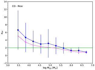
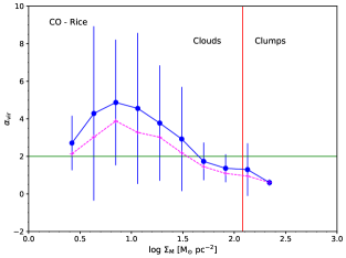
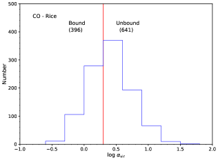
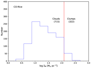
Figure 1: (Upper Left) The mean and standard deviation of the virial ratio is plotted versus the logarithm of the clump mass, for the catalog of Rice et al. (2016). Median values are plotted in a magenta dashed line. (Upper Right) The same quantities are plotted versus the mass surface density. The horizontal line at $\mbox{$\alpha_{\rm vir}$}=2$ demarcates nominally unbound clouds above the line from nominally bound clouds below the line. The vertical line in the right panel indicates $\mbox{$\Sigma_{\rm M}$}=120$ M_⊙ pc^-2. (Lower left) The histogram of values of log $\alpha_{\rm vir}$, with a vertical red line at $\mbox{$\alpha_{\rm vir}$}=2.0$. The number of structures in each category are given in parentheses. (Lower right) The histogram of values of log $\Sigma_{\rm M}$, with a vertical red line at $\mbox{$\Sigma_{\rm M}$}=120$ M_⊙ pc^-2.

We plot $\alpha_{\rm vir}$ calculated from the data in Rice et al. (2016) in Figure 1. The mean $\alpha_{\rm vir}$ declines with mass, so that $\mbox{$\langle\mbox{$\alpha_{\rm vir}$}\rangle$}<2$ for log$\mbox{$M_{\rm CO}$}>5.7$. The mean $\alpha_{\rm vir}$ also declines with $\Sigma_{\rm M}$, so that $\mbox{$\langle\mbox{$\alpha_{\rm vir}$}\rangle$}<2$ for log$\mbox{$\Sigma_{\rm M}$}>1.7$. The histograms indicate that most structures are clouds and most are

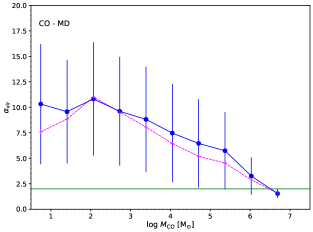
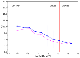
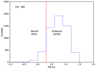
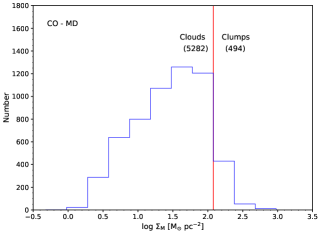
Figure 2: (Upper Left) The mean and standard deviation of the virial ratio is plotted versus the logarithm of the clump mass, for the catalog of Miville-Deschênes et al. (2017) after selecting only those catalog entries with $\mbox{$\alpha_{\rm vir}$}<100$ and $\mbox{$M_{\rm CO}$}>1$ M_⊙. Median values are plotted in a magenta dashed line. (Upper Right) The same quantities are plotted versus the mass surface density. The horizontal line at $\mbox{$\alpha_{\rm vir}$}=2$ demarcates nominally unbound clouds above the line from nominally bound clouds below the line. The vertical line in the right panel indicates $\mbox{$\Sigma_{\rm M}$}=120$ M_⊙ pc^-2. (Lower left) The histogram of values of log $\alpha_{\rm vir}$, with a vertical red line at $\mbox{$\alpha_{\rm vir}$}=2.0$. The number of structures in each category are given in parentheses. (Lower right) The histogram of values of log $\Sigma_{\rm M}$, with a vertical red line at $\mbox{$\Sigma_{\rm M}$}=120$ M_⊙ pc^-2.

The catalog of Miville-Deschênes et al. (2017), as noted in §2, contains some outliers with very high nominal $\alpha_{\rm vir}$, so we exclude those greater than a maxiumum value, $\alpha_{\rm max}$. Entries in Table 2 are given for two choices, $\mbox{$\alpha_{\rm max}$}=100$ and $\mbox{$\alpha_{\rm max}$}=20$. The mean and standard deviation are plotted versus mass in Figure 2. As we saw with the catalog of Rice et al. (2016), the $\langle\mbox{$\alpha_{\rm vir}$}\rangle$ values decline with $M_{\rm CO}$. In this case, they reach $\mbox{$\langle\mbox{$\alpha_{\rm vir}$}\rangle$}=2$ only for the most massive bin. The mean and median values of $\alpha_{\rm vir}$ decline with $\Sigma_{\rm M}$, but never drop below $\mbox{$\alpha_{\rm vir}$}=2$. The histograms indicate that the vast majority of structures are unbound clouds. The fraction of the mass that is bound is relatively insensitive to the choice of $\alpha_{\rm max}$, at about 0.19 for all structures. The fact that these results differ subtantially from those of Rice et al. (2016) will be discussed in §4.1.

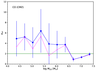
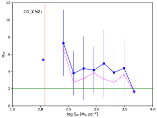
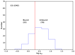
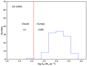
Figure 3: The catalog of Oka et al. (2001) is plotted. (Upper Left) The mean and standard deviation of the virial ratio is plotted versus the logarithm of the clump mass. Median values are plotted in a magenta dashed line. (Upper Right) The same quantities are plotted versus the mass surface density. The horizontal line at $\mbox{$\alpha_{\rm vir}$}=2$ demarcates nominally unbound clouds above the line from nominally bound clouds below the line. The vertical line indicates $\mbox{$\Sigma_{\rm M}$}=120$ M_⊙ pc^-2. (Lower left) The histogram of values of log $\alpha_{\rm vir}$, with a vertical red line at $\mbox{$\alpha_{\rm vir}$}=2.0$. The number of structures in each category are given in parentheses. (Lower right) The histogram of values of log $\Sigma_{\rm M}$, with a vertical red line at $\mbox{$\Sigma_{\rm M}$}=120$ M_⊙ pc^-2.

Figure 3 shows that the structures in the CMZ in the catalog of Oka et al. (2001) are generally unbound even though they almost all have $\mbox{$\Sigma_{\rm M}$}>120$ M_⊙ pc^-2, satisfying the local criterion for star formation. Clearly, the definition of a clump based on the local surface density criterion for active star formation does not work in the CMZ. While most structures are unbound, the tendency for higher mass structures to be bound results in a relatively high $\mbox{$f(M)$}=0.71$, with the caveat that these masses may well be overestimated (§2).

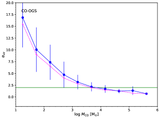
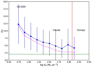
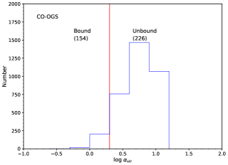
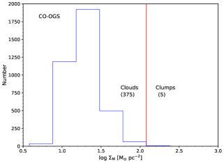
Figure 4: The catalog of Heyer et al. (2001) is plotted. The masses were limited to $\mbox{$M_{\rm CO}$}>2.5\mbox{${}\times 10^{3}$}$ M_⊙  for completeness and $\mbox{$v_{LSR}$}<-25$ km s^-1 to avoid distance ambiguity. (Upper Left) The mean and standard deviation of the virial ratio is plotted versus the logarithm of the clump mass. Median values are plotted in a magenta dashed line. (Upper Right) The same quantities are plotted versus the mass surface density. The horizontal line at $\mbox{$\alpha_{\rm vir}$}=2$ demarcates nominally unbound clouds above the line from nominally bound clouds below the line. The vertical line indicates $\mbox{$\Sigma_{\rm M}$}=120$ M_⊙ pc^-2. (Lower left) The histogram of values of log $\alpha_{\rm vir}$, with a vertical red line at $\mbox{$\alpha_{\rm vir}$}=2.0$. The number of structures in each category are given in parentheses. (Lower right) The histogram of values of log $\Sigma_{\rm M}$, with a vertical red line at $\mbox{$\Sigma_{\rm M}$}=120$ M_⊙ pc^-2.

The outer Galaxy sample (OGS) from the catalog of Heyer et al. (2001) shows a similar behavior. Most are unbound, but more than half the mass is in bound structures despite having $\mbox{$\Sigma_{\rm M}$}<120$ M_⊙ pc^-2, with $\mbox{$f(M)$}=0.72$ (Table 2). To some extent, this result depends on the requirement that $\mbox{$M_{\rm CO}$}>2.5\mbox{${}\times 10^{3}$}$ M_⊙ imposed by Heyer et al. (2001) to ensure completeness. Since completenesss is less important for our purposes, we relaxed that criterion to $\mbox{$M_{\rm CO}$}>10$ M_⊙ to see the effect. While $f(N)$ dropped to 0.06, $\mbox{$f(M)$}=0.58$, still substantial because most of the bound mass was in the higher mass structures.

3.2 Structures Defined by CO $J=2\rightarrow 1$ Emission in Other Galaxies

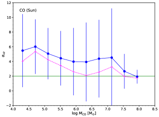
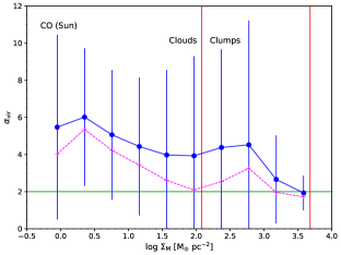
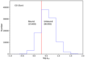
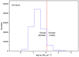
Figure 5: The mean and standard deviation of the virial ratio is plotted in bins versus the logarithm of the clump mass, for The catalog of Sun et al. (2020) is plotted. (Upper Left) The mean and standard deviation of the virial ratio is plotted versus the logarithm of the clump mass. Median values are plotted in a magenta dashed line. (Upper Right) The same quantities are plotted versus the mass surface density. The horizontal line at $\mbox{$\alpha_{\rm vir}$}=2$ demarcates nominally unbound clouds above the line from nominally bound clouds below the line. Vertical lines indicate $\mbox{$\Sigma_{\rm M}$}=120$ M_⊙ pc^-2 and $\mbox{$\Sigma_{\rm M}$}=1$ g cm^-2. (Lower left) The histogram of values of log $\alpha_{\rm vir}$, with a vertical red line at $\mbox{$\alpha_{\rm vir}$}=2.0$. The number of structures in each category are given in parentheses. (Lower right) The histogram of values of log $\Sigma_{\rm M}$, with a vertical red line at $\mbox{$\Sigma_{\rm M}$}=120$ M_⊙ pc^-2.

We were able to use all the catalog entries from table B1 of Sun et al. (2020), save one entry with a negative value for $\alpha_{\rm vir}$. Sun et al. (2020) themselves found an area-weighted median $\mbox{$\alpha_{\rm vir}$}=3.5$ with a 1-$\sigma$ spread of 0.6 dex, based on over $10^{5}$ pixels of size 150 pc in 66 galaxies. The mass-weighted median was smaller at 2.7. All the caveats about neglect of tidal effects, etc. apply quite strongly to studies with 150 pc resolution. Independent analysis of the data in their table B1 confirms the median value and finds a mean value of $\mbox{$\langle\mbox{$\alpha_{\rm vir}$}\rangle$}=4.7\pm 4.0$. The averages of $\alpha_{\rm vir}$ in Figure 5 all lie above $\mbox{$\alpha_{\rm vir}$}=2$, but they approach that value for the most massive data points. A similar pattern applies to the plot of $\alpha_{\rm vir}$ versus $\Sigma_{\rm M}$. While many points have very high $\alpha_{\rm vir}$, the fraction with $\mbox{$\alpha_{\rm vir}$}<2$ is $\mbox{$f(N)$}=0.21$ and the fraction of the total mass in those structures is $\mbox{$f(M)$}=0.35$, reflecting the usual trend for lower $\alpha_{\rm vir}$ in more massive clouds. The median and mean surface densities are 22 and 50 M_⊙ pc^-2, but with a maximum at $\mbox{$\Sigma_{\rm M}$}=9.7\mbox{${}\times 10^{3}$}$ M_⊙ pc^-2. The last value is clearly more characteristic of dense clumps, not clouds. All points above log $\mbox{$M_{\rm CO}$}=6.43$ M_⊙  correspond to $\mbox{$\Sigma_{\rm M}$}>120$ M_⊙ pc^-2 or $\mbox{$A_{V}$}>8$ mag. Vertical lines on Figure 5 indicate surface densities of 120 M_⊙ pc^-2 and 1 g cm^-2. The second of these corresponds to the criterion for massive star formation (Krumholz & McKee 2008). The fact that $\alpha_{\rm vir}$ drops to values near two as the surface density approaches this value is interesting. To have such high surface density averaged over a region of 150 pc is quite remarkable. If $\Sigma_{\rm M}$ is restricted to be less than 120 M_⊙ pc^-2, the fraction of the total mass with $\mbox{$\alpha_{\rm vir}$}<2$ becomes 0.15.

3.3 Structures Defined by ¹³CO $J=1\rightarrow 0$ Emission

To use data from all three surveys and to compare methods for structure identification, we have reanalyzed the three data sets, using the CO clouds defined by Miville-Deschênes et al. (2017) to constrain the ¹³CO voxels included. The detailed method is explained in the Appendix. However, we begin with the original catalog, but with updated abundance assumptions. These results will allow a comparison between different cloud identification methods.

3.3.1 GRS: Original Sample

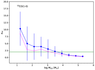
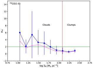
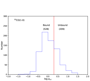
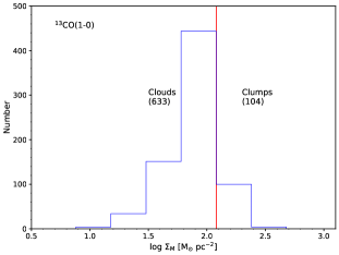
Figure 6: (Upper Left) The mean and standard deviation of the virial ratio is plotted versus the logarithm of the clump mass, for the catalog of Roman-Duval et al. (2010). after selecting only those catalog entries with $\mbox{$\Sigma_{\rm M}$}>10$ and $\mbox{$M_{\rm CO}$}>1$ M_⊙, and $\mbox{$\alpha_{\rm vir}$}<20$. Median values are plotted in a magenta dashed line. (Upper Right) The same quantities are plotted versus the mass surface density. The horizontal line at $\mbox{$\alpha_{\rm vir}$}=2$ demarcates nominally unbound clouds above the line from nominally bound clouds below the line. The vertical line in the right panel indicates $\mbox{$\Sigma_{\rm M}$}=120$ M_⊙ pc^-2. (Lower left) The histogram of values of log $\alpha_{\rm vir}$, with a vertical red line at $\mbox{$\alpha_{\rm vir}$}=2.0$. The number of structures in each category are given in parentheses. (Lower right) The histogram of values of log $\Sigma_{\rm M}$, with a vertical red line at $\mbox{$\Sigma_{\rm M}$}=120$ M_⊙ pc^-2.

The tabulated masses and surface densities for the ¹³CO GRS data from Roman-Duval et al. (2010) originally used values of H₂/CO of 12500 and $\mbox{$\mu_{\rm H_{2}}$}=2.37$. As discussed in §1, we instead use the current best values for H₂/CO and $\mu_{\rm H_{2}}$, resulting in masses and surface densities lower by a factor of 0.567 and virial parameters higher by a factor of 1.76. For a first analysis, (entry 8 in Table 2), we retain the assumption from Roman-Duval et al. (2010) of a constant CO/¹³CO of 45. The usual quantities are plotted in Figure 6 and the results are in Table 2. The majority of the sample would be classified as clouds, with $\mbox{$\Sigma_{\rm M}$}<120$ M_⊙ pc^-2, but about 1/6 are denser. The fraction of mass in bound structures, $\mbox{$f(M)$}=0.95$, but the fraction for clouds is much less, $\mbox{$f_{\rm c}(M)$}=0.55$.

3.3.2 GRS: New Analysis

From now on, we use the CO-defined structures and the ¹³CO-derived properties, with the abundance assumptions described at the end of §1, including the variation of ${\rm CO}/{\rm{}^{13}CO}$ with $R_{\rm gal}$. We begin with a re-analysis of the GRS survey in ¹³CO (Roman-Duval et al. 2010). The structures are defined in the catalog of Miville-Deschênes et al. (2017), but only for a sub-sample. The sub-sample of CO clouds is somewhat biased towards higher $\Sigma_{\rm M}$ and lower $\alpha_{\rm vir}$ than the full catalog: $\mbox{$\langle\mbox{$\Sigma_{\rm M}$}\rangle$}=95\pm 64$ M_⊙ pc^-2, nearly twice that for the full catalog; $\mbox{$\langle\mbox{$\alpha_{\rm vir}$}\rangle$}=5.62\pm 5.28$, 0.81 times that for the full catalog.

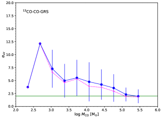
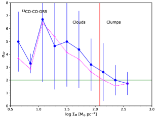
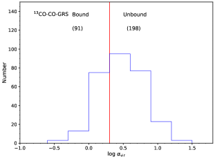
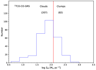
Figure 7: (Upper Left) The mean and standard deviation of the virial ratio is plotted versus the logarithm of the clump mass, for the catalog produced for the GRS in combination with CO. Median values are plotted in a magenta dashed line. (Upper Right) The same quantities are plotted versus the mass surface density. The horizontal line at $\mbox{$\alpha_{\rm vir}$}=2$ demarcates nominally unbound clouds above the line from nominally bound clouds below the line. The vertical line in the right panel indicates $\mbox{$\Sigma_{\rm M}$}=120$ M_⊙ pc^-2. The mass and surface density are the total (gas+dust) determined from submm continuum emission. (Lower left) The histogram of values of log $\alpha_{\rm vir}$, with a vertical red line at $\mbox{$\alpha_{\rm vir}$}=2.0$. The number of structures in each category are given in parentheses. (Lower right) The histogram of values of log $\Sigma_{\rm M}$, with a vertical red line at $\mbox{$\Sigma_{\rm M}$}=120$ M_⊙ pc^-2.

The analysis of the GRS data with the method described in the Appendix is listed as entry 9 of Table 2 and the usual plots are in Figure 7. The main difference from entry 8 is that the clouds were identified in the CO analysis and the ¹³CO data were taken only within the boundaries of those clouds. The change in cloud definition makes the mean $\alpha_{\rm vir}$ larger and $f(M)$ smaller by substantial amounts ($\mbox{$f(M)$}=0.46$).

The fraction of the mass of the CO-defined structure contained in the ¹³CO emission ($M_{\rm 13}/M_{\rm CO}$) is a valuable guide to the fraction of possibly bound structures within unbound CO clouds. For the GRS sample, $\mbox{$\langle\mbox{$M_{\rm 13}/M_{\rm CO}$}\rangle$}=0.22\pm 0.08$ with a median $\mbox{$M_{\rm 13}/M_{\rm CO}$}=0.21$.

3.3.3 EXFC55-100

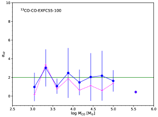
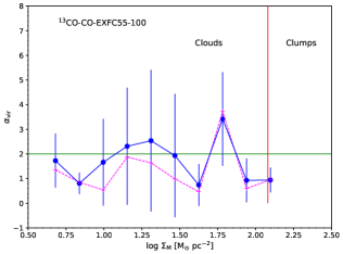
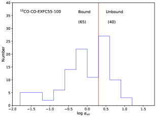
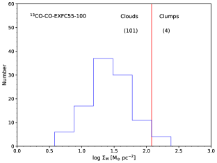
Figure 8: (Upper Left) The mean and standard deviation of the virial ratio is plotted versus the logarithm of the clump mass, for the catalog produced for the EXFC55-100 sample in combination with CO and using new abundances. Median values are plotted in a magenta dashed line. (Upper Right) The same quantities are plotted versus the mass surface density. The horizontal line at $\mbox{$\alpha_{\rm vir}$}=2$ demarcates nominally unbound clouds above the line from nominally bound clouds below the line. The vertical line in the right panel indicates $\mbox{$\Sigma_{\rm M}$}=120$ M_⊙ pc^-2. The mass and surface density are the total (gas+dust) determined from submm continuum emission. (Lower left) The histogram of values of log $\alpha_{\rm vir}$, with a vertical red line at $\mbox{$\alpha_{\rm vir}$}=2.0$. The number of structures in each category are given in parentheses. (Lower right) The histogram of values of log $\Sigma_{\rm M}$, with a vertical red line at $\mbox{$\Sigma_{\rm M}$}=120$ M_⊙ pc^-2.

For this sample, most structures are identified as clouds, but they are mostly bound, despite having low $\Sigma_{\rm M}$. The usual plots are in Figure 8 and the statistics are given as entry 10 in Table 2. The fraction of the CO mass recovered by the ¹³CO emission, $\mbox{$\langle\mbox{$M_{\rm 13}/M_{\rm CO}$}\rangle$}=0.79\pm 0.80$ with a median $\mbox{$M_{\rm 13}/M_{\rm CO}$}=0.61$. These values are much higher than those in the GRS.

3.3.4 EXFC135-195

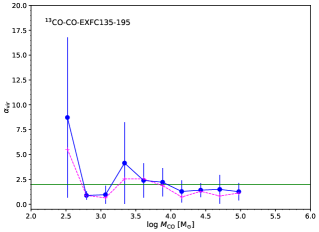
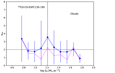
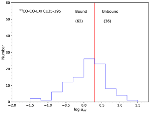
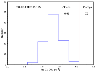
Figure 9: (Upper Left) The mean and standard deviation of the virial ratio is plotted versus the logarithm of the clump mass, for the catalog produced for the EXFC135-195 sample in combination with CO and using new abundances. Median values are plotted in a magenta dashed line. (Upper Right) The same quantities are plotted versus the mass surface density. The horizontal line at $\mbox{$\alpha_{\rm vir}$}=2$ demarcates nominally unbound clouds above the line from nominally bound clouds below the line. The vertical line in the right panel indicates $\mbox{$\Sigma_{\rm M}$}=120$ M_⊙ pc^-2. The mass and surface density are the total (gas+dust) determined from submm continuum emission. (Lower left) The histogram of values of log $\alpha_{\rm vir}$, with a vertical red line at $\mbox{$\alpha_{\rm vir}$}=2.0$. The number of structures in each category are given in parentheses. (Lower right) The histogram of values of log $\Sigma_{\rm M}$, with a vertical red line at $\mbox{$\Sigma_{\rm M}$}=120$ M_⊙ pc^-2.

As for EXFC55-100, most structures are identified as clouds, but they are mostly bound, despite having very low $\Sigma_{\rm M}$. The usual plots are in Figure 9 and the statistics are given as entry 11 in Table 2. For the EXFC135-195 sample, $\mbox{$\langle\mbox{$M_{\rm 13}/M_{\rm CO}$}\rangle$}=0.76\pm 0.34$ with a median $\mbox{$M_{\rm 13}/M_{\rm CO}$}=0.66$. These values are much higher than those in the GRS and similar to those of the EXFC55-100 sample.

3.3.5 Summary of Consequences of New Analysis

The main effect of the different method of structure identification is to decrease the fraction of mass in bound structures. In the inner Galaxy, most become unbound, but 46% of the mass is still in bound structures. For larger $R_{\rm gal}$, the structures become less dense but more bound. For the outer Galaxy (EXFC135-195) sample, $\mbox{$f(M)$}=0.75$ even though $\mbox{$\langle\mbox{$\Sigma_{\rm M}$}\rangle$}=24$ M_⊙ pc^-2. This trend reflects a strong decrease in velocity dispersion with $R_{\rm gal}$. The fraction of the mass recovered by ¹³CO ($M_{\rm 13}/M_{\rm CO}$) is low in the inner Galaxy, but quite high in the other two samples.

3.4 ¹³CO $J=2\rightarrow 1$

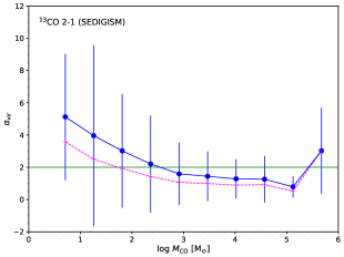
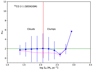
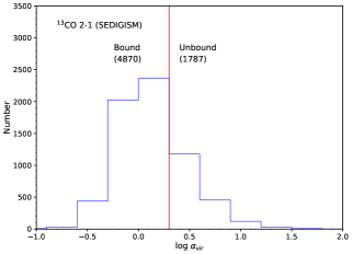
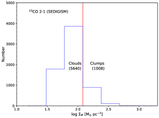
Figure 10: (Upper Left) The mean and standard deviation of the virial ratio is plotted versus the logarithm of the clump mass, for the catalog of Duarte-Cabral et al. (2021), after selecting only those catalog entries with good distances, not on edges and at least 114 pixels. Median values are plotted in a magenta dashed line. (Upper Right) The same quantities are plotted versus the mass surface density. The horizontal line at $\mbox{$\alpha_{\rm vir}$}=2$ demarcates nominally unbound clouds above the line from nominally bound clouds below the line. The vertical line in the right panel indicates $\mbox{$\Sigma_{\rm M}$}=120$ M_⊙ pc^-2. (Lower left) The histogram of values of log $\alpha_{\rm vir}$, with a vertical red line at $\mbox{$\alpha_{\rm vir}$}=2.0$. The number of structures in each category are given in parentheses. (Lower right) The histogram of values of log $\Sigma_{\rm M}$, with a vertical red line at $\mbox{$\Sigma_{\rm M}$}=120$ M_⊙ pc^-2.

The situation for the $J=2\rightarrow 1$ transition of ¹³CO (Duarte-Cabral et al. 2021), shown in Figure 10, is different. Most clouds defined in this sample are nominally bound, even for relatively low mass and $\Sigma_{\rm M}$. However, $\langle\mbox{$\alpha_{\rm vir}$}\rangle$ is lower and $f(M)$ is higher than for the $J=1\rightarrow 0$ in the GRS sample with the new analysis, but comparable for the other $J=1\rightarrow 0$ samples.

3.5 Stuctures Defined by Herschel and NH₃

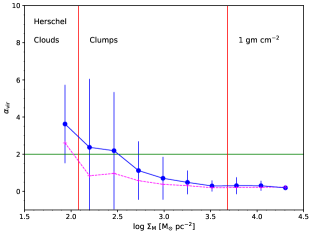
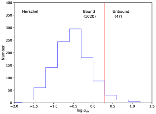
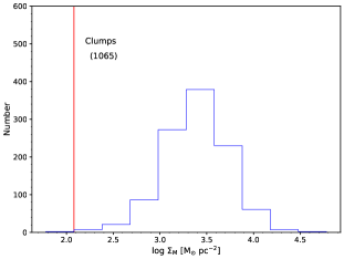
Figure 11: (Upper Left) The mean and standard deviation of the virial ratio is plotted versus the logarithm of the clump mass, for the catalog of Merello et al. (2019). Median values are plotted in a magenta dashed line. (Upper Right) The same quantities are plotted versus the mass surface density. The horizontal line at $\mbox{$\alpha_{\rm vir}$}=2$ demarcates nominally unbound clouds above the line from nominally bound clouds below the line. The vertical lines in the right panel indicate $\mbox{$\Sigma_{\rm M}$}=120$ M_⊙ pc^-2 and $\mbox{$\Sigma_{\rm M}$}=1$ g cm^-3. The mass and surface density are the total (gas+dust) determined from submm continuum emission. (Lower left) The histogram of values of log $\alpha_{\rm vir}$, with a vertical red line at $\mbox{$\alpha_{\rm vir}$}=2.0$. The number of structures in each category are given in parentheses. (Lower right) The histogram of values of log $\Sigma_{\rm M}$, with a vertical red line at $\mbox{$\Sigma_{\rm M}$}=120$ M_⊙ pc^-2.

Compact structures identified by their submm emission with Herschel have very low virial parameters, strongly indicative of being gravitationally dominated and $\mbox{$f(M)$}=1.0$. Figure 11 plots the virial parameter versus the logarithm of clump mass from an analysis by Merello et al. (2019). Only the clumps with the lowest mass and $\Sigma_{\rm M}$ are unbound. While most of these contain star formation, even the 157 “prestellar” clumps are strongly gravitationally dominated, with $\mbox{$\langle\mbox{$\alpha_{\rm vir}$}\rangle$}=0.57$, almost identical to the value for the full sample. The values for $f_{\rm c}(N)$ and $f_{\rm c}(M)$ of zero reflect the fact that the very few structures in the sample with surface densities small enough to be considered clouds are all unbound.

4 Discussion

In this section, we will explore how the boundedness of structures depends on methods and properties. We include sub-sections on the method used to identify structures, the tracer used to define the structures and measure the mass, the location in the Galaxy, mass of the structure, and the surface density of the structure.

4.1 Dependence on Method Used to Identify Structure

The first issue to consider is the fact that the results from two different decompositions of the CO $J=1\rightarrow 0$ survey by Dame et al. (2001) show quite different results. The difference is clear from the Figures, but it can be encapsulated in the values of $f(M)$: the structures identified by Rice et al. (2016) have $\mbox{$f(M)$}=0.73$ while those of Miville-Deschênes et al. (2017) have $\mbox{$f(M)$}=0.19$.

Clearly, the choice of method to identify structures plays a major role in the different results. We can borrow the terminology of taxonomists to distinguish lumpers and splitters. In our context, lumpers would aggregate emission into larger structures, while splitters would break emission into smaller structures. Rice et al. (2016) used a dendrogram analysis to identify 1064 clouds, accounting for about 25% of the molecular mass in the Galaxy. They note that their method avoids merging unrelated clouds into pseudo-clouds. In this sense, they are splitters. Comparing their catalog to that of Dame et al. (1986) (based on an early version of the first quadrant survey), they recover all of the same clouds, but some are split and less massive. They use the size-linewidth relation and latitude distribution to break the kinematic distance ambiguity. In contrast, Miville-Deschênes et al. (2017) might reasonably be called lumpers. They performed a Gaussian decomposition of each spectrum and then lumped them together by a clustering procedure. This process led to larger linewidths in the clouds (median $\mbox{$\sigma_{v}$}=3.6$ km s^-1) than in the individual Gaussian components (median $\mbox{$\sigma_{v}$}=1.65$ km s^-1). Interestingly, this method allowed them to identify 98% of the CO emission with 8107 clouds. They found that the size-linewidth relation has too much scatter, so they use the relation $\mbox{$\sigma_{v}$}\propto(R\mbox{$\Sigma_{\rm M}$})^{0.5}$, where $R$ is the cloud size, to resolve the kinematic distance ambiguity. While the mass also increased by this process, the net effect was probably to produce larger $\alpha_{\rm vir}$. Were they lumpers or splitters? In the sense that they aggregated velocity components, they were lumpers, but they decomposed four times as much of the CO emission into 8 times as many clouds as Rice, making them splitters. Lumping in velocity and splitting in number of clouds is likely to lead to larger $\alpha_{\rm vir}$. However, the fact that the scaling relation mentioned above holds indicates that unrelated gas is not being lumped in pseudo-clouds.

Another difference between the results of the two methods is apparent in the x-axis values for the plots of $\alpha_{\rm vir}$ versus $M_{\rm CO}$. The plot for Rice et al. (2016) starts at $\log\mbox{$M_{\rm CO}$}=3.5$, while that of Miville-Deschênes et al. (2017) starts at $\log\mbox{$M_{\rm CO}$}=0.5$. The latter catalog contains many more clouds of lower mass. However, this does not explain the difference in $f(M)$ because the total mass is still dominated by the massive clouds.

Probably the main factor in the difference is the completeness in accounting for the CO emission of the Galaxy. Because Rice et al. (2016) account for only 25% of the CO emission, their catalog is less suitable for addressing the question of slow star formation on the Galactic scale, where the problem was defined by taking the total mass of molecular gas from the CO survey and dividing by a free-fall time.

In this context, the data from Sun et al. (2020) are interesting as no method is used to define structures. Instead only the mass within a 150 pc region is tabulated. The fact that $\mbox{$f(M)$}=0.35$ and $\mbox{$f_{\rm c}(M)$}=0.15$, averaged over many galaxies and galactocentric radii, even with some very high values for $\Sigma_{\rm M}$, suggests that the most likely value for $f(M)$ is relatively small for structures measured by CO, regardless of which of the two transitions is used.

The importance of the identification method is also apparent in the difference between the results from the original structures in the Roman-Duval et al. (2010) GRS sample (entry 8 in Table 2) and the new analysis, where structures were defined by the CO catalog of Miville-Deschênes et al. (2017) (entry 9 in Table 2).

These differences suggest that procedures like CLUMPFIND or dendrogram analyses tend to split structures or minimize low level, extended emission. For addressing the global issue of slow star formation, procedures that account for all the emission are necessary.

4.2 Dependence on the Tracer Used to Define Structure

We begin with the extremes: the samples of Miville-Deschênes et al. (2017) and Sun et al. (2020) showing low values for $f(M)$ for mass measured from CO emission, versus the sample of Merello et al. (2019) showing $\mbox{$f(M)$}=1.0$ for structures traced by Herschel peaks and NH₃ linewidths. The distinction between clouds, primarily traced by CO, and dense clumps, primarily traced by peaks in submillimeter emission and lines of species rarer than CO, has been based on this difference, but the analysis of $\alpha_{\rm vir}$ strongly supports this distinction. The much higher mean and median $\Sigma_{\rm M}$ for the Herschel-NH₃ data also indicate that these are clearly distinct structures.

What about the structures probed by ¹³CO? They clearly lie between the extremes of clouds and dense clumps. For the GRS sample with our new analysis, $\mbox{$f(M)$}=0.46$ and $\mbox{$\langle\mbox{$\alpha_{\rm vir}$}\rangle$}=3.83$ and $\mbox{$\langle\mbox{$\Sigma_{\rm M}$}\rangle$}=104$. For the sample defined by ¹³CO $J=2\rightarrow 1$, from (Duarte-Cabral et al. 2021), $\mbox{$f(M)$}=0.79$ and $\mbox{$\langle\mbox{$\alpha_{\rm vir}$}\rangle$}=1.94$, even though $\mbox{$\langle\mbox{$\Sigma_{\rm M}$}\rangle$}=87.7$ M_⊙ pc^-2, lower than that of ¹³CO $J=1\rightarrow 0$ in the GRS, but higher than that of ¹³CO $J=1\rightarrow 0$ in the other two surveys.

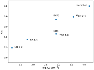
Figure 12: The value of $f(M)$ versus $n_{\rm eff}$ of the tracer. The higher point for ¹³CO $J=1\rightarrow 0$ is for the average of the two EXFC surveys, while the lower point is from the analysis in this paper for the GRS survey. Both points for ¹³CO $J=1\rightarrow 0$ use the structures in the CO catalog of Miville-Deschênes et al. (2017).

The trend with tracer is that $\alpha_{\rm vir}$ decreases (structures are more likely to be bound) as the tracer changes from CO to ¹³CO $J=1\rightarrow 0$ to ¹³CO $J=2\rightarrow 1$ to Herschel-NH₃. This can be related to a trend in the characteristic density of the material being traced. The characteristic density probed by each tracer can be crudely estimated from the effective density of the tracer used to define the structure. The effective density ($n_{\rm eff}$), defined by Evans (1999) and developed further by Shirley (2015), is the density of particles needed to produce a 1 K km s^-1 observed line for an assumed column density and kinetic temperature. Because effective densities for CO and ¹³CO were not calculated by those references, we calculated them using the on-line tool RADEX (van der Tak et al. 2007) assuming $\mbox{$T_{K}$}=10$ K and column density corresponding to $\mbox{$A_{V}$}=1$ mag, so $N({\rm CO})=1\mbox{${}\times 10^{17}$}$ cm^-2 and $N(\mbox{${}^{13}$CO})=1.7\mbox{${}\times 10^{15}$}$ cm^-2. The resulting effective densities are 15, 60, 800, 3800 cm^-3 for CO $J=1\rightarrow 0$, CO $J=2\rightarrow 1$, ¹³CO $J=1\rightarrow 0$, ¹³CO $J=2\rightarrow 1$, respectively. The comparable density for the Herschel sample is less clear. The structures were identified from dust continuum emission, but NH₃ observations of both (1,1) and (2,2) inversion transitions were required in order to estimate the kinetic temperature, $T_{K}$. The effective density for the (2,2) line at $\mbox{$T_{K}$}=15$ K is $\mbox{$n_{\rm eff}$}=1.6\mbox{${}\times 10^{4}$}$ cm^-3 (Shirley 2015), similar to the density of about 2${}\times 10^{4}$ cm^-3 needed to make $T_{K}$ close to the dust temperature, $T_{d}$, as found by Merello et al. (2019). We take $\mbox{$n_{\rm eff}$}=1.6\mbox{${}\times 10^{4}$}$ for the Herschel sample.

The values for $f(M)$ are plotted versus these effective densities in Figure 12. We use only the results for entries 3, 7, 9, 12, and 13, along with the average of 10 and 11 (the EXFC samples), from Table 2 as most representative of structure selection by each tracer. Clearly the fraction of the mass in bound structures increases rapidly with $n_{\rm eff}$, reaching values about 0.8 for densities near the effective density of ¹³CO $J=2\rightarrow 1$ and unity for the Herschel sample. The data roughly follow a line in the semilog plot, but the two points for ¹³CO $J=1\rightarrow 0$ suggest that location in the Galaxy also matters.

4.3 Dependence on Location in the Galaxy

The contrast between the inner Galaxy (CMZ) (Oka et al. 2001) and the outer Galaxy (OGS) (Heyer et al. 2001) is perhaps the most striking. The structures identified in the CMZ have very high surface densities ($\mbox{$\langle\mbox{$\Sigma_{\rm M}$}\rangle$}=1700$ M_⊙ pc^-2), but $\mbox{$f(M)$}=0.71$. In contrast the structures in the OGS have very low surface densities ($\mbox{$\langle\mbox{$\Sigma_{\rm M}$}\rangle$}=17.7$ M_⊙ pc^-2), but $\mbox{$f(M)$}=0.58$ for entry 6, with the more inclusive lower limit on cloud mass. With the criterion of $\mbox{$\Sigma_{\rm M}$}<120$ M_⊙ pc^-2, none of the structures in the CMZ defined by CO are bound (both $f_{\rm c}(N)$ and $f_{\rm c}(M)$ are zero), while $\mbox{$f_{\rm c}(M)$}=0.46$ or 0.56 in the OGS, depending on the mass limits used. Clearly, the local criterion of $\mbox{$\Sigma_{\rm M}$}=120$ M_⊙ pc^-2 for boundedness, based on a star formation threshold, is inappropriate for these parts of the Galaxy. In the CMZ, a clump would need to be defined with a much higher $\Sigma_{\rm M}$, higher than 3000 M_⊙ pc^-2. In the outer Galaxy, the opposite applies.

A difficulty with this comparison is that very different criteria were used to define structures in the CMZ compared to the disk or outer Galaxy. A high threshold was needed to isolate structures in the highly confused CMZ. Using the same procedure for all $R_{\rm gal}$, Miville-Deschênes et al. (2017) did not find a drop in median of $\alpha_{\rm vir}$ at large $R_{\rm gal}$, but did see a rise inside a few kpc. The sample of other galaxies (Sun et al. 2020) also uses a common method for all radii. There are 1562 data points in their catalog with $\mbox{$R_{\rm gal}$}<0.5$ kpc, similar to the definition of the CMZ in the Milky Way. In that restricted sample, the median, mean, and standard deviation of $\Sigma_{\rm M}$ are 130, 375, 670 M_⊙ pc^-2, much higher than the full sample, but still less than those for the CMZ. The median, mean, and standard deviation of $\alpha_{\rm vir}$ are 5.45, 8,28, 9.03, about twice those for the full sample, and larger than those for the CMZ, while the fractions in bound structures are $\mbox{$f(N)$}=0.11$ and $\mbox{$f(M)$}=0.27$, substantially smaller than for the full sample or for the CMZ of the Milky Way. The data from other galaxies supports the idea that a much higher surface density is needed to produce bound structures in the inner regions of galaxies and suggests that most of the molecular gas there is unbound despite very high surface densities.

Comparing the GRS and EXFC samples in ¹³CO $J=1\rightarrow 0$ reveals a similar pattern. More mass is in bound structures despite the lower $\Sigma_{\rm M}$ in the outer parts of the Galaxy.

4.4 Dependence on Mass

A trend common to all the samples is a decrease in $\alpha_{\rm vir}$ with increasing mass. At some level, this trend is a result of a trend of decreasing $\alpha_{\rm vir}$ with increasing $\Sigma_{\rm M}$. This is most obvious for the sample of Sun et al. (2020), where the size of the region considered is constant, so the trend with mass is really a trend with surface density.

Contrary evidence that the most massive clouds may be unbound can be seen in Figure 8 from Dame et al. (1986) who consider the 26 most massive complexes in the first quadrant of the Milky Way. About half have linewidths larger than those expected from virial equilibrium. A more recent analysis of the most massive complexes by Nguyen-Luong et al. (2016) found that most were unbound. While some are engaged in what they called “mini-starbursts” which could be unbinding the cloud, those sources do not have a very different distribution of virial parameters. It is these very large complexes that will dominate studies of CO in other galaxies. They also dominate the total mass of molecular gas in our Galaxy because the cloud mass function slope is less than 2, unlike the case for stars. However, the mass function peaks at much lower masses in the outer Galaxy, as shown in Figure 7 of Miville-Deschênes et al. (2017). A similar trend is seen for molecular clouds in M33 (Rosolowsky 2005).

4.5 Dependence on Mass Surface Density

The decrease in median and mean $\alpha_{\rm vir}$ with increasing $\Sigma_{\rm M}$ is clear from the relevant plots for most samples that cover the relevant range of $\Sigma_{\rm M}$. The distinction between clouds and clumps adopted for discussion in this paper is $\mbox{$\Sigma_{\rm M}$}=120$ M_⊙ pc^-2. To explore this connection further, we have calculated the mass fraction in bound structures in bins of 0.3 in log $\Sigma_{\rm M}$ for samples that cover the transition well. As shown in Figure 13, these all show a strong increase in the fraction of mass that is bound as $\Sigma_{\rm M}$ increases.

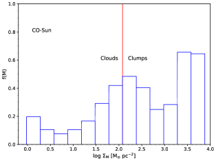
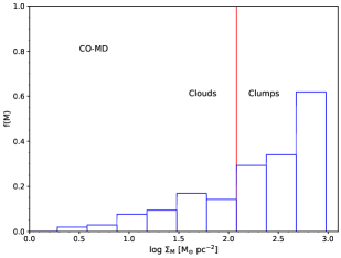
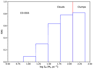
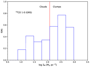
Figure 13: The value of $f(M)$ is plotted versus log $\Sigma_{\rm M}$ for the CO samples of Sun et al. (2020), Miville-Deschênes et al. (2017), Heyer et al. (2001), and the ¹³CO $J=1\rightarrow 0$ sample for the GRS, with structures identified by CO (entry 9 in Table 2).

The dependence on surface density is also reflected in the values of $f_{\rm c}(N)$ and $f_{\rm c}(M)$ in Table 2. These are generally smaller than the $f(N)$ and $f(M)$ computed for all structures. Only a small fraction of the gas in structures we have called clouds is bound. This statement applies both to Milky Way structures and to those in other galaxies.

The decline of virial parameter with mass may in part be an artifact of observational biases in the way that the linewidth is measured (Traficante et al. 2018). They point out that the tracers used for determining the velocity dispersion may be weighted more heavily to denser regions, with smaller dispersions that do not reflect the full dispersion of the entire structure. This effect would be most noticeable in samples for which the tracers of mass and velocity dispersion are different. The effect might contribute to the very low values of $\alpha_{\rm vir}$ and the strong trend with mass in the Herschel sample.

4.6 Caveats and Uncertainties

As discussed extensively in §1, there are substantial uncertainties in computing the virial parameter. For any given structure, the uncertainty in $\alpha_{\rm vir}$ is likely to be a factor of 2 or 3. Analyses of the uncertainties in estimating cloud mass, velocity dispersion, etc. can be found in Beaumont et al. (2013). Masses from CO luminosities have uncertainties, as discussed in the introduction, so that we expect uncertainties of at least a factor of 3, and these may be systematic uncertainties, at least in the case of $M_{\rm CO}$. Gong et al. (2018) argue that X(CO) may be overestimated based on “observing” simulations. They get a value of X(CO) about half the standard value of 2${}\times 10^{20}$. If that is correct, masses from CO would be overestimated and virial parameters underestimated. Finally, we re-emphasize the dependence on the method used to define a cloud.

For ¹³CO, our newer analysis accounts for the latest measurements of the isotopic ratio, ${\rm CO}/{\rm{}^{13}CO}$, as a function of $R_{\rm gal}$ and the latest value of H₂/CO. On the other hand, we have made no correction for changes in the CO abundance with metallicity, which is known to decrease with $R_{\rm gal}$. Deharveng et al. (2000) found a gradient in the oxygen abundance gradient over the range of 5-15 kpc: $12+\log{\rm O/H}=(-3.95\pm 0.49)\mbox{${}\times 10^{-2}$}\mbox{$R_{\rm gal}$}+(8.82\pm 0.05)$. The effect of metallicity on CO emission is not simple, but extragalactic observers commonly use a correction factor: $\mbox{$\alpha_{\rm CO}$}=4.35Z^{-1.6}$ M_⊙(K km s^-1pc²)^-1 (Sun et al. 2020 and references therein), where $Z$ is the metallicity relative to solar. If we applied the same correction factor, CO clouds at 3 kpc would have twice higher $\alpha_{\rm vir}$, while those at 15 kpc would have about one-third the value of $\alpha_{\rm vir}$. Such a correction would strengthen the already strong trend for clouds to be unbound in the inner Galaxy, where most of the molecular mass resides, and to be bound in the outer Galaxy.

We reiterate that methods of structure identification remain one of the most significant sources of uncertainty.

5 Consequences for the Star Formation Rate Problem

The results of this analysis have consequences for the problem of the star formation rate, discussed in the introduction. If only a fraction of the mass of molecular gas in the Galaxy is in bound structures, the over-prediction of the star formation rate of 300 M_⊙ yr^-1, can be decreased substantially. Based on the catalog of Miville-Deschênes et al. (2017), only 19% of structures defined by CO $J=1\rightarrow 0$ are bound, decreasing the theoretical star formation rate to 57 M_⊙ yr^-1, using the same assumption about the free-fall time as the value found in §1.

We can make a more accurate estimate by assessing the star formation rate cloud by cloud, then adding those rates up. If we assume that only clouds with $\mbox{$\alpha_{\rm vir}$}\leq 2$ form stars in a free fall time based on the mean density of that cloud, the predicted star formation rate for an individual cloud is

$$\mbox{$SFR_{\rm th}$}=M/\mbox{$t_{\rm ff}$}=6.04\mbox{${}\times 10^{-8}$}M_{\mbox{M${}_{\odot}$}}^{1.5}r_{\rm pc}^{-1.5}$$ (10)

Using the catalog of Miville-Deschênes et al. (2017) because it accounts for all the molecular clouds defined by CO emission, and summing the star formation rate only over bound clouds, we find a total star formation rate for the Milky Way of 46.4 M_⊙ yr^-1, a factor of 6.5 less than the value in the introduction. This is mostly due to the small fraction of bound clouds, but there is also a contribution from a longer $t_{\rm ff}$ because the mean density of the clouds identified by Miville-Deschênes et al. (2017) is less than 100 cm^-3. The resulting depletion time of bound molecular gas is decreased to $\mbox{$t_{\rm dep}$}=1.0\mbox{${}\times 10^{8}$}$ yr, closer to the free-fall time, but still considerably larger.

Of course, regions of clouds are likely to be bound even if the entire cloud is not. The fraction of bound mass could be assessed from comparison of masses indicated by different tracers. Ideally, we would do the same analysis for a complete survey of the Galaxy in other tracers, especially ¹³CO. A similar calculation for the ¹³CO GRS survey, using the full sample (entry 8 in Table 2) predicts a star formation rate of 7.4 M_⊙ yr^-1. However, the existing ¹³CO surveys do not cover the whole Galaxy, and the new analysis was possible only for a subset of the ¹³CO data, so we cannot do a direct calculation. Instead we calculate the fraction of the mass of the unbound CO-defined structures that is found in the bound ¹³CO-derived properties. This value is $0.22$ for the GRS, which applies to the inner Galaxy, which contains most of the molecular mass. The fraction is higher (0.77-0.80) in the outer parts of the Galaxy. So this material would increase the predicted star formation rate. If all of the ¹³CO-derived mass in the unbound CO-defined clouds in the GRS sample form stars at the fiducial $t_{\rm ff}$, they would contribute another 55 M_⊙ yr^-1 to the Galactic star formation rate. Clearly, a full sky survey of ¹³CO would be very valuable.

We have focused on $\epsilon_{\rm ff}$, rather than the final efficiency ($\epsilon_{\rm sf}$) Because the most massive clouds seem most likely to be bound (subject to the caveats above), the difference between mass functions of clouds and clusters is, if anything, increased. The resolution to this problem may lie in the inclusion of tidal forces since most of these very massive clouds reside in the inner Galaxy.

6 Conclusions

We list the main conclusions before discussing them:

1. Clearly, the choice of method to identify clouds plays a major role in the different results.

2. The tracer (both molecule and transition) that is used to define structures has a strong effect on whether those structures are bound.

3. At a fixed $R_{\rm gal}$, the fraction of the mass in bound structures increases rapidly with the effective density of the tracer, suggesting that regions with larger volume densities contribute more to bound gas.

4. Many clouds identified by CO are unbound and most of the mass in those clouds is unbound.

5. Structures defined by dust continuum emission and linewidths from NH₃ emission are almost all bound.

6. Structures defined by ¹³CO emission are more likely to be bound than those defined by CO emission. However, their boundedness also depends on the method used to identify them and on assumptions about isotopic and elemental abundances.

7. Boundedness correlates strongly with surface density.

8. Structures within 0.5 kpc of a galaxy center have much higher surface density, but much of the mass is unbound because of higher turbulence. The opposite is true in outer regions.

9. More generally, structures identified by CO or ¹³CO have lower surface density, but are more likely to be bound, at larger $R_{\rm gal}$.

10. More massive clouds are more likely to be bound, but this trend is partially confused with the trend with surface density.

11. For the most complete catalog of structures traced by CO (Miville-Deschênes et al. 2017), the fraction of mass in bound structures, $\mbox{$f(M)$}=0.19$, alleviating, but not eliminating, the fundamental problem of slow star formation in the Milky Way.

The most important conclusion is that most of the mass traced by CO emission is in unbound structures. This result was anticipated by theorists, notably Dobbs et al. (2011), whose title asked “Why are most molecular clouds not gravitationally bound?”. Their answer involved cloud-cloud collisions and stellar feedback; shredding and merging resulted in clouds not being well-defined entities with the same gas over cloud “lifetimes.” Padoan et al. (2017) argued that supernova feedback kept the interstellar medium sufficiently stirred up that many structures were unbound even though their densities were such that they were likely molecular. As mentioned in §1, Kim et al. (2021) found that unbound clouds are needed to reach the observational constraints on the star formation rate.

Observers have often found, but seldom emphasized, this result. Roman-Duval et al. (2016) suggested that gas detected in CO, but not ¹³CO might be “diffuse, non-star-forming gas,” but did not explicitly suggest that this gas was unbound. Figure 16 of Miville-Deschênes et al. (2017) already showed that almost all the structures in their catalog are unbound, but this result was not particularly emphasized. Nguyen-Luong et al. (2016) showed that mini-starburst complexes, which have enhanced star formation rate density, are actively forming massive stars but are not necessarily bound, suggesting that being bound is not the major factor regulating their star formation activity. The idea that structures identified by molecular emission are well-defined, bound structures, unlike the more diffuse atomic interstellar medium, is long-standing and creates cognitive dissonance with contrary factual evidence. Uncertainties are often invoked to argue that clouds are bound even when the evidence suggests otherwise (see Dobbs et al. 2011 for discussion of this tendency.). However, there is no good reason to believe that the atomic-molecular transition is identical to the unbound-bound transition. This would be plausible if most of the support were thermal, but it is turbulent (Zuckerman & Evans 1974). The fact that these transitions are close can be coincidental (see pg. 36 of Elmegreen 1985) and may have led us astray.

$$T_{13}(x,y,v)^{\prime}=F(X,Y,v)T_{13}(x,y,v)$$ (1)

where $X-dX/2<x<X+dX/2$, $Y-dY/2<y<Y+dY/2$, and $dX$, $dY$ are the 0.125 degree pixel sizes of the CO data cube. The effect of this multiplication is to suppress any contribution to the integrated ¹³CO emission from signal outside of the CO velocity interval, as shown in Figure 14.

The cloud mass is computed from $N(\mbox{{\rm H}${}_{2}$})$ found from equation 10 in §1 as follows:

$$M(\mbox{${}^{13}$CO})=\mbox{$\mu_{\rm H_{2}}$}m_{\rm H}D^{2}\int d\Omega N(\mbox{{\rm H}${}_{2}$})(l,b)$$ (2)

where $\mbox{$\mu_{\rm H_{2}}$}=2.8$, $m_{\rm H}$ is the atomic hydrogen mass, and $D$ is the distance to the cloud. For each cloud, the velocity dispersion, $\sigma_{v}$(¹³CO) and cloud radius are calculated following Miville-Deschênes et al. (2017). Both $\sigma_{v}$(¹³CO) and radius are deconvolved from the native spectral and angular resolutions of the data. We also deconvolved the CO velocity dispersions and cloud sizes. Clouds are excluded from any subsequent analyses if either the cloud size or velocity dispersion is not resolved. Finally, the ¹³CO-derived virial mass is derived from Equation 8. Accounting for these selection criteria, there are 289 clouds from the GRS, 105 clouds from the EXFC55-100 survey, and 98 clouds from the EXFC135-195 survey.

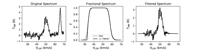
Figure 14: The method used to filter unrelated signal from ¹³CO. The spectrum on the left is the original data. The center panel shows the function that isolates the velocity range that is consistent with that of the CO-defined structure. The right panel shows the filtered ¹³CO spectrum that contributes to the ¹³CO-defined mass and other properties.

References

- Accurso et al. (2017) Accurso, G., Saintonge, A., Catinella, B., et al. 2017, MNRAS, 470, 4750, doi: 10.1093/mnras/stx1556
- Astropy Collaboration et al. (2013) Astropy Collaboration, Robitaille, T. P., Tollerud, E. J., et al. 2013, A&A, 558, A33, doi: 10.1051/0004-6361/201322068
- Astropy Collaboration et al. (2018) Astropy Collaboration, Price-Whelan, A. M., Sipőcz, B. M., et al. 2018, AJ, 156, 123, doi: 10.3847/1538-3881/aabc4f
- Beaumont et al. (2013) Beaumont, C. N., Offner, S. S. R., Shetty, R., Glover, S. C. O., & Goodman, A. A. 2013, ApJ, 777, 173, doi: 10.1088/0004-637X/777/2/173
- Benjamin et al. (2003) Benjamin, R. A., Churchwell, E., Babler, B. L., et al. 2003, PASP, 115, 953, doi: 10.1086/376696
- Bertoldi & McKee (1992) Bertoldi, F., & McKee, C. F. 1992, ApJ, 395, 140, doi: 10.1086/171638
- Bigiel et al. (2008) Bigiel, F., Leroy, A., Walter, F., et al. 2008, AJ, 136, 2846, doi: 10.1088/0004-6256/136/6/2846
- Bolatto et al. (2013) Bolatto, A. D., Wolfire, M., & Leroy, A. K. 2013, ARA&A, 51, 207, doi: 10.1146/annurev-astro-082812-140944
- Brunt et al. (2009) Brunt, C. M., Heyer, M. H., & Mac Low, M. M. 2009, A&A, 504, 883, doi: 10.1051/0004-6361/200911797
- Chomiuk & Povich (2011) Chomiuk, L., & Povich, M. S. 2011, AJ, 142, 197, doi: 10.1088/0004-6256/142/6/197
- Churchwell et al. (2009) Churchwell, E., Babler, B. L., Meade, M. R., et al. 2009, PASP, 121, 213, doi: 10.1086/597811
- Clemens et al. (1986) Clemens, D. P., Sanders, D. B., Scoville, N. Z., & Solomon, P. M. 1986, ApJS, 60, 297, doi: 10.1086/191087
- Colombo et al. (2019) Colombo, D., Rosolowsky, E., Duarte-Cabral, A., et al. 2019, MNRAS, 483, 4291, doi: 10.1093/mnras/sty3283
- Dame et al. (1986) Dame, T. M., Elmegreen, B. G., Cohen, R. S., & Thaddeus, P. 1986, ApJ, 305, 892, doi: 10.1086/164304
- Dame et al. (2001) Dame, T. M., Hartmann, D., & Thaddeus, P. 2001, ApJ, 547, 792, doi: 10.1086/318388
- Deharveng et al. (2000) Deharveng, L., Peña, M., Caplan, J., & Costero, R. 2000, MNRAS, 311, 329, doi: 10.1046/j.1365-8711.2000.03030.x
- Dickman (1978) Dickman, R. L. 1978, ApJS, 37, 407, doi: 10.1086/190535
- Dobbs et al. (2011) Dobbs, C. L., Burkert, A., & Pringle, J. E. 2011, MNRAS, 413, 2935, doi: 10.1111/j.1365-2966.2011.18371.x
- Duarte-Cabral et al. (2021) Duarte-Cabral, A., Colombo, D., Urquhart, J. S., et al. 2021, MNRAS, 500, 3027, doi: 10.1093/mnras/staa2480
- Elia et al. (2017) Elia, D., Molinari, S., Schisano, E., et al. 2017, MNRAS, 471, 100, doi: 10.1093/mnras/stx1357
- Elmegreen (1985) Elmegreen, B. G. 1985, in Protostars and Planets II, ed. D. C. Black & M. S. Matthews, 33–58
- Evans (1999) Evans, Neal J., I. 1999, ARA&A, 37, 311, doi: 10.1146/annurev.astro.37.1.311
- Evans et al. (2014) Evans, Neal J., I., Heiderman, A., & Vutisalchavakul, N. 2014, ApJ, 782, 114, doi: 10.1088/0004-637X/782/2/114
- Gildas Team (2013) Gildas Team. 2013, GILDAS: Grenoble Image and Line Data Analysis Software. http://ascl.net/1305.010
- Gong et al. (2018) Gong, M., Ostriker, E. C., & Kim, C.-G. 2018, ApJ, 858, 16, doi: 10.3847/1538-4357/aab9af
- Gong et al. (2020) Gong, M., Ostriker, E. C., Kim, C.-G., & Kim, J.-G. 2020, ApJ, 903, 142, doi: 10.3847/1538-4357/abbdab
- Grudić et al. (2019) Grudić, M. Y., Hopkins, P. F., Lee, E. J., et al. 2019, MNRAS, 488, 1501, doi: 10.1093/mnras/stz1758
- Heiderman et al. (2010) Heiderman, A., Evans, Neal J., I., Allen, L. E., Huard, T., & Heyer, M. 2010, ApJ, 723, 1019, doi: 10.1088/0004-637X/723/2/1019
- Heigl et al. (2018) Heigl, S., Gritschneder, M., & Burkert, A. 2018, MNRAS, 481, L1, doi: 10.1093/mnrasl/sly146
- Heyer & Dame (2015) Heyer, M., & Dame, T. M. 2015, ARA&A, 53, 583, doi: 10.1146/annurev-astro-082214-122324
- Heyer et al. (1998) Heyer, M. H., Brunt, C., Snell, R. L., et al. 1998, ApJS, 115, 241, doi: 10.1086/313086
- Heyer & Brunt (2004) Heyer, M. H., & Brunt, C. M. 2004, ApJ, 615, L45, doi: 10.1086/425978
- Heyer et al. (2001) Heyer, M. H., Carpenter, J. M., & Snell, R. L. 2001, ApJ, 551, 852, doi: 10.1086/320218
- Jackson et al. (2006) Jackson, J. M., Rathborne, J. M., Shah, R. Y., et al. 2006, ApJS, 163, 145, doi: 10.1086/500091
- Jacob et al. (2020) Jacob, A. M., Menten, K. M., Wiesemeyer, H., et al. 2020, A&A, 640, A125, doi: 10.1051/0004-6361/201937385
- Kauffmann et al. (2008) Kauffmann, J., Bertoldi, F., Bourke, T. L., Evans, N. J., I., & Lee, C. W. 2008, A&A, 487, 993, doi: 10.1051/0004-6361:200809481
- Kauffmann et al. (2013) Kauffmann, J., Pillai, T., & Goldsmith, P. F. 2013, ApJ, 779, 185, doi: 10.1088/0004-637X/779/2/185
- Kawamura et al. (2009) Kawamura, A., Mizuno, Y., Minamidani, T., et al. 2009, ApJS, 184, 1, doi: 10.1088/0067-0049/184/1/1
- Kim et al. (2018) Kim, J.-G., Kim, W.-T., & Ostriker, E. C. 2018, ApJ, 859, 68, doi: 10.3847/1538-4357/aabe27
- Kim et al. (2021) Kim, J.-G., Ostriker, E. C., & Filippova, N. 2021, ApJ, 911, 128, doi: 10.3847/1538-4357/abe934
- Krumholz & McKee (2008) Krumholz, M. R., & McKee, C. F. 2008, Nature, 451, 1082, doi: 10.1038/nature06620
- Krumholz et al. (2014) Krumholz, M. R., Bate, M. R., Arce, H. G., et al. 2014, in Protostars and Planets VI, ed. H. Beuther, R. S. Klessen, C. P. Dullemond, & T. Henning, 243, doi: 10.2458/azu_uapress_9780816531240-ch011
- Lacy et al. (2017) Lacy, J. H., Sneden, C., Kim, H., & Jaffe, D. T. 2017, ApJ, 838, 66, doi: 10.3847/1538-4357/aa6247
- Lada & Dame (2020) Lada, C. J., & Dame, T. M. 2020, ApJ, 898, 3, doi: 10.3847/1538-4357/ab9bfb
- Lada et al. (2012) Lada, C. J., Forbrich, J., Lombardi, M., & Alves, J. F. 2012, ApJ, 745, 190, doi: 10.1088/0004-637X/745/2/190
- Lada et al. (2010) Lada, C. J., Lombardi, M., & Alves, J. F. 2010, ApJ, 724, 687, doi: 10.1088/0004-637X/724/1/687
- Larson (1981) Larson, R. B. 1981, MNRAS, 194, 809, doi: 10.1093/mnras/194.4.809
- Lee et al. (2021) Lee, J. C., Whitmore, B. C., Thilker, D. A., et al. 2021, arXiv e-prints, arXiv:2101.02855. https://arxiv.org/abs/2101.02855
- Mac Low (1999) Mac Low, M.-M. 1999, ApJ, 524, 169, doi: 10.1086/307784
- Mao et al. (2020) Mao, S. A., Ostriker, E. C., & Kim, C.-G. 2020, ApJ, 898, 52, doi: 10.3847/1538-4357/ab989c
- Massey et al. (1995) Massey, P., Johnson, K. E., & Degioia-Eastwood, K. 1995, ApJ, 454, 151, doi: 10.1086/176474
- McKee & Williams (1997) McKee, C. F., & Williams, J. P. 1997, ApJ, 476, 144, doi: 10.1086/303587
- Merello et al. (2019) Merello, M., Molinari, S., Rygl, K. L. J., et al. 2019, MNRAS, 483, 5355, doi: 10.1093/mnras/sty3453