Rodrigues’ descendants of a polynomial and Boutroux curves

Abstract.

Motivated by the classical Rodrigues’ formula, we study below the root asymptotic of the polynomial sequence

$$\mathcal{R}_{[\alpha n],n,P}(z)=\frac{\mathop{}\!\mathrm{d}^{[\alpha n]}P^{n}(z)}{\mathop{}\!\mathrm{d}z^{[\alpha n]}},n=0,1,\dots$$

where ${P(z)}$ is a fixed univariate polynomial, $\alpha$ is a fixed positive number smaller than $\deg P$, and $[\alpha n]$ stands for the integer part of $\alpha n$.

Our description of this asymptotic is expressed in terms of an explicit harmonic function uniquely determined by the plane rational curve emerging from the application of the saddle point method to the integral representation of the latter polynomials using Cauchy’s formula for higher derivatives. As a consequence of our method, we conclude that this curve is birationally equivalent to the zero locus of the bivariate algebraic equation satisfied by the Cauchy transform of the asymptotic root-counting measure for the latter polynomial sequence. We show that this harmonic function is also associated with an abelian differential having only purely imaginary periods and the latter plane curve belongs to the class of Boutroux curves initially introduced in [Be, BM]. As an additional relevant piece of information, we derive a linear ordinary differential equation satisfied by $\{\mathcal{R}_{[\alpha n],n,P}(z)\}$ as well as higher derivatives of powers of more general functions.

platt och avintetgjord
släpar jag nollan min
vid håret
in i oändlighet.
(Ur “I grund och botten”,
Majken Johansson, 195$6^{1}$)

1. Introduction

Around 1816 (Benjamin) Olinde Rodrigues discovered his famous formula

$$P_{n}(z)=\frac{1}{2^{n}n!}\frac{\mathop{}\!\mathrm{d}^{n}}{\mathop{}\!\mathrm{d}z^{n}}\left((z^{2}-1)^{n}\right)$$ (1.1)

for the Legendre polynomials which undoubtedly became a standard tool in the toolbox of classical orthogonal polynomials and special functions, see e.g. [AbSt]. (Later this formula was also rediscovered by Sir J. Ivory and C. G. Jacobi, see [As].)

Among other properties, the $n$-th Legendre polynomial $P_{n}(z)$ satisfies the linear ordinary differential equation

$$(1-z^{2})y^{\prime\prime}-2zy^{\prime}+n(n+1)y=0,$$ (1.2)

and the asymptotic of the zeros as $n\to\infty$ is described by classical results.

1.1. Main Problem

Imitating Rodrigues’ approach, given a polynomial $P$ of degree $d\geq 1$, let us consider a double-indexed family of polynomials determined by the Rodrigues-like expression

$$\mathcal{R}_{m,n,P}(z):=\ \frac{\mathop{}\!\mathrm{d}^{m}}{\mathop{}\!\mathrm{d}z^{m}}\left(P^{n}(z)\right),\;n=0,1,\dots\text{ and }m=0,1,\dots,nd.$$

These polynomials which we below call Rodrigues’ descendants of $P$ were apparently for the first time considered by N. Ciorânescu in 1933 (see [Ci]) where he, in particular, derived linear differential equations satisfied by them. In 1965, and, to the best of our knowledge, independently of N. Ciorânescu’s work a linear differential equation satisfied by $\mathcal{R}_{n,n,P}(z)$ has been (re)discovered by J. M. Horner, (see [Ho]).

If $P=z^{2}-1$ and $m=n$, we get the above classical case of the Legendre polynomials up to a scalar factor. In Fig.  2 we display the zeros of $\mathcal{R}_{m,n,P}(z)$ for some choices of $P$.

In the present paper, we study the asymptotic root distribution for natural sequences of Rodrigues’ descendants of $P$. (There is a straightforward generalization of our set-up to the case of rational/meromorphic $P$ which we plan to adress in a future publication.)

1.2. Main results

In what follows, we will always assume that a polynomial $P(z)$ under consideration satisfies the condition $d:=\deg P\geq 2$. The remaining case $d\leq 1$ is trivial.

For any polynomial $P$ and its Rodrigues’ descendant $\mathcal{R}_{m,n,P}(z),$ denote by $\mu_{m,n,P}$ the root-counting measure of $\mathcal{R}_{m,n,P}(z)$ and by

$$\mathcal{C}_{m,n,P}(z):=\frac{\mathcal{R}^{\prime}_{m,n,P}(z)}{(dn-m)\cdot\mathcal{R}_{m,n,P}(z)}$$

the Cauchy transform of $\mu_{m,n,P}$, see (2.2). Note that $dn-m=\deg\mathcal{R}_{m,n,P}$. (For the basic notions of the logarithmic potential theory such as the Cauchy transform $\mathcal{C}_{\mu}$ and the logarithmic potential $L_{\mu}$ of a measure $\mu$ supported in $\mathbb{C}$ consult § 2.2 and [Ra].)

We say that a polynomial $P$ is strongly generic if both $P$ and $P^{\prime}$ have simple roots.

Theorem 1.1.

For any strongly generic polynomial $P$ and a given positive number $\alpha<\deg P$, there exists a weak limit

$$\mu_{\alpha,P}:=\lim_{n\to\infty}\mu_{[\alpha n],n,P}.$$

Moreover, its Cauchy transform $\mathcal{C}_{\alpha,P}$ defined as the pointwise limit

$$\mathcal{C}:=\mathcal{C}_{\alpha,P}(z):=\lim_{n\to\infty}\mathcal{C}_{[\alpha n],n,P}(z)$$

exists almost everywhere (a.e.) in $\mathbb{C}$ and satisfies the algebraic equation

$$(d-\alpha)\mathcal{C}=\frac{\mathop{}\!\mathrm{d}}{\mathop{}\!\mathrm{d}z}\log{P}\left(z+\frac{\alpha}{(d-\alpha)\mathcal{C}}\right).$$ (1.3)

Remark 1.2.

Observe that, by the Gauss-Lucas theorem, for any $0<\alpha<d,$ the support $S_{\alpha,P}$ of $\mu_{\alpha,P}$ is contained in the convex hull of the zero locus of $P$.

Remark 1.3.

The condition of strong genericity is apparently redundant and is an artefact of our particular proofs.

Reinterpretation of formula (1.3) in Theorem 1.1 implies the following result.

Corollary 1.4.

The Cauchy transform $\mathcal{C}:=\mathcal{C}_{\alpha,P}(z)$ of the limiting measure $\mu_{\alpha,P}$ satisfies the equation

$$\sum_{k=0}^{d}\frac{\alpha^{k-1}\,(\alpha-k)(d-\alpha)^{d-k}}{k!}\,P^{(k)}\mathcal{C}^{d-k}=0.$$ (1.4)

Example 1.5.

(i) For $P=z^{2}+az+b$, equation (1.4) reduces to

$$(2-\alpha)(z^{2}+az+b)\mathcal{C}^{2}+(\alpha-1)(2z+a)\mathcal{C}-\alpha=0.$$ (1.5)

(ii) For $P=z^{3}+az^{2}+bz+c$, it reduces to

$$(3-\alpha)^{2}(z^{3}+az^{2}+bz+c)\mathcal{C}^{3}+(\alpha-1)(3-\alpha)(3z^{2}+2az+b)\mathcal{C}^{2}+\alpha(\alpha-2)(3z+a)\mathcal{C}-\alpha^{2}=0.$$ (1.6)

Remark 1.6.

Observe that equations (1.3) and (1.4) will substantially simplify if instead of the above Cauchy transform $\mathcal{C}$ one uses its scaled version $\mathcal{W}$ introduced in (3.1), see § 3.

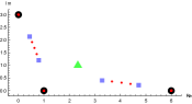
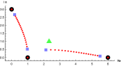
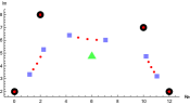
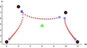
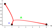
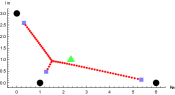
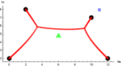
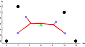
Figure 1. The zeros of $\mathcal{R}_{m,60,P}(z)$ shown by the small red dots. (The larger dots are the zeros of $P$, the triangle is the center of mass of the zero locus of $P$, and the squares are branch points of (1.4) and (3.2) in the $z$-plane when $\alpha=m/60$.) Both in the left and in the right subfigures, $m=3$ (top left), $m=18$ (top right), $m=60$ (bottom left), and $m=60(\deg{P}-1)$ (bottom right).

The next theorem is our main technical result on the asymptotic limit of the above root-counting measures. (Although several notions in its formulation are explicated only later in the text we want to give a reader the flavour of our results.)

Set

$$H(z,u):=\frac{1}{d-\alpha}(\log|P(u)|-\alpha\log|u-z|).$$ (1.7)

Let $\pi:\mathbb{C}_{z}\times\mathbb{C}_{u}\to\mathbb{C}_{z}$ be the standard projection, and $\mathcal{D}\subset\mathbb{C}_{z}\times\mathbb{C}_{u}$ be the saddle point curve of $H$, see details in § 4.2. ($\mathcal{D}$ is a rational curve defined by an explicit algebraic equation (3.11) whose coefficients depend on $P$ and $\alpha$.) Further, let $U_{rel}\subset\mathcal{D}$ be the open set of relevant saddle points, see § 4.2. Denote by $\tilde{\pi}:U_{rel}\to O\subset\mathbb{C}_{z}$ the restriction of $\pi$ to $U_{rel}$ and define the tropical trace $\tilde{\pi}_{*}H(z):O\to\mathbb{R}\cup\pm\infty$ as a piecewise-harmonic function obtained by taking the fiberwise maximum of $H(z,u)$, see § 2.3. (We will show that $\tilde{\pi}_{*}H(z)$ is an $L^{1}_{loc}$-function defined on the dense and open subset $O\subset\mathbb{C}_{z}$, see Prop. 4.9. Since the complement of $\mathbb{C}_{z}\setminus O$ is a zero set, $\tilde{\pi}_{*}H(z)$ extends to a subharmonic $L^{1}_{loc}$-function on the whole $\mathbb{C}_{z}$.)

Theorem 1.7.

In the above notation, for any strongly generic polynomial $P$ of degree $d\geq 2$, there exists a real number $B$ (explicitly calculated in Lemma 4.10) such that

$$\lim_{n\to\infty}L_{\mu_{[\alpha n],n,P}}(z)=B+\tilde{\pi}_{*}H(z),$$

where the above relation is understood as the equality of $L^{1}_{loc}$-functions. Here $L_{\mu}$ stands for the logarithmic potential of a measure $\mu$, see (2.1). Consequently,

$$\lim_{n\to\infty}\mathcal{C}_{\mu_{[\alpha n],n,P}}(z)=2\frac{\partial}{\partial z}\tilde{\pi}_{*}H(z),$$

and

$$\lim_{n\to\infty}\mu_{[\alpha n],n,P}=\mu_{\alpha,P}:=\frac{2}{\pi}\frac{\partial^{2}}{\partial z\partial\bar{z}}\tilde{\pi}_{*}H(z),$$

where the latter two limits are understood in the sense of distributions and $\mu_{\alpha,P}$ is a positive measure.

Theorem 1.7 combined with the definition of the tropical trace provide important general information about the support of the measure $\mu_{\alpha,P}$, e.g., that it consists of certain level curves of explicit harmonic functions associated with the above function $H(z,u)$ together with the algebraic function defined by the saddle point curve, see Theorems 2.9 – 2.23. Fig. 1 and  2 show several illustrations of (approximations to) the supports of the measures $\mu_{\alpha,P}$ and their union taken over $0<\alpha<\deg P$.

Remark 1.8.

We want to mention that the previous theorems remain true for any sequence of Rodrigues descendants $\{\mathcal{R}_{a_{n},n,P}(z)\}$ such that $\lim_{n\to\infty}a_{n}/n=\alpha$. (The only changes in our proofs needed to cover this case are setting $m:=a_{n}$ and $s_{n}:=n-a_{n}/\alpha$ in the proof in § 4, and observing that $s_{n}/n\to 0$ as $n\to\infty$, so that Corollary A applies, and finally checking that Lemma 4.10 still is valid.) We want to thank an anonymous referee for suggesting this generalization.

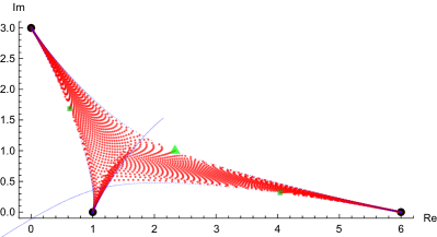
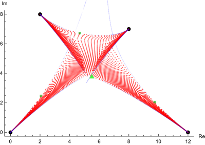
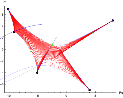
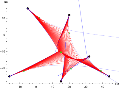
Figure 2. The union of all zeros of $\mathcal{R}_{m,30,P}(z)$ for $m=0,1,$ $\dotsc,30\deg{P}-1$ shown by small red dots. (Other symbols have the same meaning as in Fig. 1.)

1.3. Methods

Let us first sketch the proof of the main technical result Theorem 1.7, from which many other results are formal consequences. Cauchy’s formula for higher order derivatives gives

$$\mathfrak{q}_{n}(z)=\frac{([\alpha n]-1)!}{2\pi i}\int_{c}\frac{P^{n}(u)\,\mathop{}\!\mathrm{d}u}{(u-z)^{[\alpha n]}}=\frac{([\alpha n]-1)!}{2\pi i}\int_{c}\mathrm{exp}\bigg{(}n\log P(u)-([\alpha n]\log(u-z)\bigg{)}\mathop{}\!\mathrm{d}z.$$ (1.8)

Here $c$ is any simple closed curve in $\mathbb{C}$ encircling $z$ once in the counterclockwise direction. The saddle point method heuristically implies that

$$\frac{1}{n}\log\mathfrak{q}_{n}(z)\approx\log P(u)-\alpha\log(u-z),$$

where $u(z)$ is some solution of the saddle point equation

$$\frac{P^{\prime}(u)}{P(u)}-\frac{\alpha}{u-z}=0,$$

determining the critical points of the integrand. The degree of the polynomial $\mathfrak{q}_{n}(z)$ equals $d_{n}:=dn-[\alpha n]+1$. Therefore, up to scaling, $\frac{1}{n}Re\,(\log\mathfrak{q}_{n}(z))$ equals the logarithmic potential $\{L_{\mu_{n}}(z)\}$ of the root-counting measure $\mu_{n}$, which we hence understand asymptotically.

The main difficulty in making the above sketch rigorous is to describe which particular branch $u(z)$ of solution to the latter saddle point equation to choose. We address this issue by applying to our specific situation a general framework developed in § 2.2. We hope that this framework can be useful in other asymptotic questions involving sequences of polynomials originating from families of linear ordinary differential equations.

Namely, given $\mathbb{C}^{2}\simeq\mathbb{C}_{z}\times\mathbb{C}_{u}$ with coordinates $(z,u)$, we define below a special class of plane algebraic curves which we call affine Boutroux curves (shorthand aBc). Such a curve $\Upsilon\subset\mathbb{C}^{2}$ is characterized by the fact that the standard $1$-form $u\hskip 0.50003pt\mathop{}\!\mathrm{d}z$ has only imaginary periods on the normalization of the compactification of $\Upsilon$ in $\mathbb{C}P^{1}_{z}\times\mathbb{C}P^{1}_{u}$.

A version of Boutroux curves has been earlier introduced in [BM] where also the term “Boutroux curves” was coined. This notion was further elaborated in [Be] and later used by a number of authors.

Given an affine Boutroux curve, we define on it a natural harmonic function which is essentially the real part of a primitive function of $u\hskip 0.50003pt\mathop{}\!\mathrm{d}z$, as well as the push-forward of this function to $\mathbb{C}P^{1}_{z}$. This push-forward —which we call the tropical trace, and which is our crucial tool—is piecewise-harmonic and its Laplacian (considered as a $2$-current on $\mathbb{C}P^{1}_{z}$) is a signed measure supported on a finite union of segments of analytic curves and isolated points. The most essential property of this measure is that its Cauchy transform satisfies almost everywhere (a.e.) in $\mathbb{C}P^{1}_{z}$ the same algebraic equation which defines the initial affine Boutroux curve. We will also apply this construction to certain open (in the usual topology) subsets of a Boutroux curve.

The structure of the paper is as follows. After recalling some basic notions in § 2.1, we introduce in §§ 2.2 – 2.7 affine Boutroux curves (aBc) as well as related harmonic functions, tropical traces and their measures. In particular, we give a simple general construction of Boutroux curves, of which the one used in this paper is a special case. In § 3, we prove that the algebraic curves given by (1.4) and (3.2) are affine Boutroux curves. In § 4, we settle Theorems 1.1 and 1.7 and related results by applying the saddle point method to Cauchy’s integral, in a very classical way. In § 5, we derive linear differential equations satisfied by Rodrigues’ descendants. In § 6, we discuss in detail the case of a quadratic polynomial $P$. Finally, in § 7, we suggest a generalization of our set-up to non-discrete measures and pose a number of open problems related to the asymptotic of Rodrigues descendants.

Remark 1.9.

This text has been mainly written, but for various reasons not completely finished already in Spring 2018; its content has been presented during a workshop “Hausdorff geometry of polynomials and polynomial sequences” at the Mittag-Leffler institute in Stockholm. Since then several relevant papers discussing similar questions about the behavior of roots of polynomials under consecutive differentiations appeared, see e.g., [St1, St2, HoKa, KiTa]. In particular, paper [St2] contains a heuristic deduction of an intriguing partial differential equation satisfied (under several additional assumptions) by the density of roots under differentiation. This equation has been further studied in [KiTa]. In addition, a recent contribution [HoKa] contains a number of results in the case of polynomials of degree $2$ which are quite close to those in our § 6.

Acknowledgements. The authors are sincerely grateful to the Mittag-Leffler institute for the hospitality in June 2018. The third author wants to thank Professors Arno Kuijlaars, Maurice Duits, Zakhar Kabluchko, and Andrei Martínez-Finkelshtein for their interest in this subject and discussions. The first author wants to thank Helga Lundholm for her support and interest in this project. Finally, we are very grateful to the anonymous referees for their high quality comments which enabled us to improve the content as well as the exposition of the paper.

2. Various preliminaries

2.1. Basics of logarithmic potential theory

For the convenience of our readers, let us briefly recall some notions and facts used throughout the text. Let $\mu$ be a finite compactly supported positive Borel measure in the complex plane $\mathbb{C}$. Define the logarithmic potential of $\mu$ as

$$L_{\mu}(z):=\int_{\mathbb{C}}\ln|z-\xi|\,\mathop{}\!\mathrm{d}\mu(\xi)$$ (2.1)

and the Cauchy transform of $\mu$ as

$$\mathcal{C}_{\mu}(z):=\int_{\mathbb{C}}\frac{\mathop{}\!\mathrm{d}\mu(\xi)}{z-\xi}.$$ (2.2)

Standard facts about the logarithmic potential and the Cauchy transform include the following.

• $\mathcal{C}_{\mu}$ and $L_{\mu}$ are locally integrable; in particular they define distributions on $\mathbb{C}$ and therefore can be acted upon by $\frac{\partial}{\partial z}$ and $\frac{\partial}{\partial\bar{z}}.$

• $\mathcal{C}_{\mu}$ is analytic in the complement of the support of $\mu$ considered in $\mathbb{C}P^{1}\simeq\mathbb{C}\cup\{\infty\}$. For example, if $\mu$ is supported on the unit circle, then $\mathcal{C}_{\mu}$ is analytic both inside the open unit disc and outside the closed unit disc.

• The main relations between $\mu$, $\mathcal{C}_{\mu}$ and $L_{\mu}$ are as follows:

  $$\mathcal{C}_{\mu}=2\frac{\partial L_{\mu}}{\partial z}\quad\text{and}\quad\mu=\frac{1}{\pi}\frac{\partial\mathcal{C}_{\mu}}{\partial\bar{z}}=\frac{2}{\pi}\frac{\partial^{2}L_{\mu}}{\partial z\partial\bar{z}}=\frac{1}{2\pi}\left(\frac{\partial^{2}L_{\mu}}{\partial x^{2}}+\frac{\partial^{2}L_{\mu}}{\partial y^{2}}\right).$$

  (They should be understood as equalities of distributions.)

• The Laurent series of $\mathcal{C}_{\mu}$ in a neighborhood of $\infty$ is given by

  $$\mathcal{C}_{\mu}(z)=\frac{m_{0}(\mu)}{z}+\frac{m_{1}(\mu)}{z^{2}}+\frac{m_{2}(\mu)}{z^{3}}+\ldots,$$

  where

  $$m_{k}(\mu)=\int_{\mathbb{C}}z^{k}\,\mathop{}\!\mathrm{d}\mu(z),\;k=0,1,\dots$$

  are the harmonic moments of the measure $\mu$.

Given a polynomial $p$, we associate to $p$ its standard root-counting measure

$$\mu_{p}=\frac{1}{\deg p}\sum_{i}m_{i}\delta(z_{i}),$$

where the sum is taken over all distinct roots $z_{i}$ of $p$ and $m_{i}$ is the multiplicity of $z_{i}$. Here $\delta(a)$ stands for the standard Dirac measure supported at $a$.

One can easily check that the Cauchy transform of $\mu_{p}$ is given by

$$\mathcal{C}_{\mu_{p}}=\frac{1}{\deg p}\cdot\frac{p^{\prime}}{p}.\quad$$

For more relevant information on the Cauchy transform we recommend the short and well-written treatise [Ga].

The above notions of a Borel measure $\mu$ compactly supported in $\mathbb{C}$, its logarithmic potential $L_{\mu}$, and its Cauchy transform $\mathcal{C}_{\mu}$ have natural extensions to $\mathbb{C}P^{1}\supset\mathbb{C}$; we denote these extensions as $\bar{\mu},\bar{L}_{\bar{\mu}},\bar{\mathcal{C}}_{\bar{\mu}}$ respectively. (The main relations between them will be preserved under such extension.) These notions are constructed as follows.

(i) For a finite positive measure $\mu$ compactly supported in $\mathbb{C}$, we introduce the signed measure $\bar{\mu}$ of total mass $0$ defined on $\mathbb{C}P^{1}$ by adding to $\mu$ the point measure $-\mathfrak{m}\cdot\delta(\infty)$ placed at $\infty$, where $\mathfrak{m}=\int_{\mathbb{C}}\mathop{}\!\mathrm{d}\mu$. (It is natural to think of $\bar{\mu}$ as an exact $2$-current on $\mathbb{C}P^{1}$.)

(ii) The logarithmic potential $L_{\mu}$ is originally defined as a function on $\mathbb{C}\subset\mathbb{C}P^{1}$ with a logarithmic singularity at $\infty$. In terms of a local coordinate $w=1/z$ at $\infty$ the logarithmic potential is a $L^{1}_{loc}$-function near $\infty$ which implies that we can define its derivatives (at least in the sense of distributions). We denote by $\bar{L}_{\bar{\mu}}$ the function $L_{\mu}$ considered as a $L^{1}_{loc}$-function on the whole $\mathbb{C}P^{1}$.

Recall that on any complex manifold, the exterior differential $\mathop{}\!\mathrm{d}$ (acting on differential forms and currents) is standardly decomposed as $\mathop{}\!\mathrm{d}=\mathop{}\!\mathrm{d}^{\prime}+\mathop{}\!\mathrm{d}^{\prime\prime}$, where $\mathop{}\!\mathrm{d}^{\prime}$ is its holomorphic and $\mathop{}\!\mathrm{d}^{\prime\prime}$ is its anti-holomorphic parts. For a function $f$ on a Riemann surface with a local holomorphic coordinate $z$, we get

$$\mathop{}\!\mathrm{d}^{\prime}f=\frac{\partial f}{\partial z}\mathop{}\!\mathrm{d}z\quad\text{and}\quad\mathop{}\!\mathrm{d}^{\prime\prime}f=\frac{\partial f}{\partial\bar{z}}\mathop{}\!\mathrm{d}\bar{z}.$$

In the above notation, the quantities $\bar{\mu}$ and $\bar{L}_{\bar{\mu}}$ satisfy the relation

$$\bar{\mu}\,\mathop{}\!\mathrm{d}x\wedge\mathop{}\!\mathrm{d}y=\frac{i}{\pi}\mathop{}\!\mathrm{d}^{\prime}\mathop{}\!\mathrm{d}^{\prime\prime}\bar{L}_{\bar{\mu}}.$$

More explicitly, we have that

$$\bar{\mu}\hskip 0.50003pt\mathop{}\!\mathrm{d}x\wedge\mathop{}\!\mathrm{d}y=\frac{1}{2\pi}\left(\frac{\partial^{2}\bar{L}_{\bar{\mu}}}{\partial x^{2}}+\frac{\partial^{2}\bar{L}_{\bar{\mu}}}{\partial y^{2}}\right)\,\mathop{}\!\mathrm{d}x\wedge\mathop{}\!\mathrm{d}y=\frac{2}{\pi}\frac{\partial^{2}\bar{L}_{\bar{\mu}}}{\partial z\partial\bar{z}}\,\mathop{}\!\mathrm{d}x\wedge\mathop{}\!\mathrm{d}y=\frac{i}{\pi}\frac{\partial^{2}\bar{L}_{\bar{\mu}}}{\partial z\partial\bar{z}}\,\mathop{}\!\mathrm{d}z\wedge\mathop{}\!\mathrm{d}\bar{z},$$

where $\frac{\partial^{2}\bar{L}_{\bar{\mu}}}{\partial z\partial\bar{z}}$ is understood as a distribution on $\mathbb{C}P^{1}$.

(iii) Finally, the Cauchy transform $\bar{\mathcal{C}}_{\bar{\mu}}$ is naturally interpreted as a $1$-current defined by the relation

$$\bar{\mathcal{C}}_{\bar{\mu}}=2\mathop{}\!\mathrm{d}^{\prime}\bar{L}_{\bar{\mu}}=2\frac{\partial\bar{L}_{\bar{\mu}}}{\partial z}\,\mathop{}\!\mathrm{d}z.$$

With this convention we get

$$\bar{\mu}\hskip 0.50003pt\mathop{}\!\mathrm{d}x\wedge\mathop{}\!\mathrm{d}y=\frac{i}{\pi}\mathop{}\!\mathrm{d}^{\prime}\mathop{}\!\mathrm{d}^{\prime\prime}\bar{L}_{\bar{\mu}}=-\frac{i}{2\pi}\mathop{}\!\mathrm{d}^{\prime\prime}\bar{\mathcal{C}}_{\bar{\mu}}=\frac{i}{2\pi}\frac{\partial\bar{C}_{\bar{\mu}}}{\partial\bar{z}}\,\mathop{}\!\mathrm{d}z\wedge\mathop{}\!\mathrm{d}\bar{z}.$$

2.2. Differentials with imaginary periods

To settle Theorem 1.1 and other related results, we need to introduce a special class of plane algebraic curves and show how they give rise to measures on (open subsets of) $\mathbb{C}P^{1}$. This is an instance of a more general construction which can be carried out for Riemann surfaces endowed with an abelian differential and a meromorphic function.

Typically multi-valued (harmonic and subharmonic) functions on Riemann surfaces originate from the integration of meromorphic $1$-forms. For some special types of differentials however, one can get functions that are uni-valued instead of multi-valued which is exactly the situation which we want to capture.

As usual, by a period of a meromorphic $1$-form on a Riemann surface $Y$ we mean the integral of this form over a $1$-cycle in $H_{1}(Y\setminus Pol,\mathbb{R})$, where $Pol$ is the set of poles of the form under consideration.

Definition 2.1.

A meromorphic $1$-form $\omega$ defined on a compact orientable Riemann surface $Y$ is said to have purely imaginary periods if all of its periods are purely imaginary complex numbers.

Remark 2.2.

Observe that the periods of $\omega$ can be roughly subdivided into two different types: a) periods related to the poles of $\omega,$ i.e. integrals of $\omega$ over small loops surrounding the poles, and b) periods related to the non-trivial $1$-dimensional homology classes of $Y$, i.e., integrals of $\omega$ over the global cycles in $H_{1}(Y,\mathbb{R})$. (Observe however that these two types of periods are, in general, dependent.)

Note that the first type of periods are purely imaginary if and only if all residues of $\omega$ are real and that the second type of periods do not occur if $Y$ has genus $0$.

Remark 2.3.

In some situations Definition 2.1 makes sense even if $Y$ is a non-compact Riemann surface. For our purposes, it will be suffficient to consider the case when $Y$ is an open subset of a compact Riemann surface $\widetilde{Y}$ such that $\widetilde{Y}\setminus Y$ consists of a finite number of points. This will always be the case for, e.g., smooth quasi-affine plane algebraic curves. Note that a meromorphic $1$-form $\omega$ on $\widetilde{Y}$ has purely imaginary periods if and only if the restriction of $\omega$ to $Y$ has purely imaginary periods.

For a meromorphic $1$-form $\omega$ with purely imaginary periods defined on a compact Riemann surface $Y$, denote by $Pol_{\omega}^{-}\subset Y$ (resp. $Pol_{\omega}^{+}\subset Y$) the set of all poles of $\omega$ with negative (resp. positive) residues. Set $Pol_{\omega}:=Pol_{\omega}^{+}\cup Pol_{\omega}^{-}$.

Meromorphic $1$-forms, i.e., abelian differentials with purely real periods were introduced by I. Krichever in the 1980’s in connection with the theory of integrable systems and have been discussed since then in a number of his papers. In particular, they were considered in [GrKr] where they were used to study the moduli spaces of Riemann surfaces with marked points. (In the present article we consider purely imaginary periods, but the translation is trivial.) One of the results of [GrKr] is as follows; see Proposition 3.4 in loc. cit.

Proposition A.

For any compact Riemann surface $Y$, a set of marked points $p_{1},\dots,p_{n}\in Y$, any set of positive integers $h_{1},\dots,h_{n}$, any choice of $h_{i}$-jets of local coordinates $z_{i}$ in the neighborhood of marked points $p_{i}$, of the singular parts (i.e., for $i=1,\dots,n,$ the choice of Taylor coefficients $c^{1}_{i},\dots,c^{h_{i}}_{i}$, with all imaginary residues $c_{i}^{1}\in i\mathbb{R}$ and the sum of the residues $\sum c_{i}^{1}$ vanishing), there exists a unique differential $\Psi$ on $Y$ with purely real periods and prescribed singular parts. In other words, in a neighborhood $U_{i}$ of each $p_{i}$ the differential $\Psi$ satisfies the condition

$$\Psi|_{U_{i}}=\sum_{j=1}^{h_{i}}c_{i}^{j}\frac{\mathop{}\!\mathrm{d}z}{z_{i}^{j}}+O(1).$$

Proposition A implies that on an arbitrary compact Riemann surface $Y$ there exists a large class of meromorphic $1$-forms with purely imaginary periods.

Furthermore, we can associate to each meromorphic differential with imaginary periods on $Y$ a real-valued function $Y\setminus Pol_{\omega}\to\mathbb{R}$ as follows. Fix a point $p_{0}\in Y\setminus Pol_{\omega}$ and consider the multi-valued primitive function

$$\Psi(p):=\int_{p_{0}}^{p}\omega.$$

$\Psi(p)$ is a well-defined uni-valued function on the universal covering of $Y\setminus Pol_{\omega}$. The next statement is trivial.

Lemma 2.4.

In the above notation, $\omega$ has purely imaginary periods on $Y$ if and only if the multi-valued primitive function $\Psi(p)$ has a uni-valued real part $\mathrm{Re}\,\Psi(p)$. In other words,

$$H(p):=\mathrm{Re}\,\Psi(p)$$

is a well-defined uni-valued function on $Y\setminus Pol_{\omega}$.

Note that $H(p)$ is continuous and harmonic in a neighborhood of any point in $Y\setminus Pol_{\omega}$. The local behavior of $H$ near a pole $p$ is determined by the sign of the residue of $\omega$ at $p$. Namely, let $\omega$ be a meromorphic $1$-form with purely imaginary periods and only simple poles. For $p\in Pol_{\omega}$, let $z$ be a local coordinate at $p$, and denote by $r$ the residue of $\omega$ at $p$.

Lemma 2.5.

In the above notation, $H$ is a subharmonic $L^{1}_{loc}$-function on $Y\setminus Pol_{\omega}^{-}$ which is harmonic on $Y\setminus Pol_{\omega}$. Locally, for the restriction of $H$ to a suitable neighborhood of $p$, the following holds:

1. $H(z)=r\log|z|+\widetilde{H}(z)$, where $\widetilde{H}(z)$ is a function harmonic in a neighborhood of $p$. Consequently, $\frac{\partial^{2}H}{\partial z\partial\bar{z}}=\frac{r\pi}{2}\delta(p)$, where $\delta(p)$ is the Dirac measure at $p$, and the derivatives are taken in the sense of distributions.

2. If $p\in Pol_{\omega}^{+}$, then there is a neighborhood of $p$ in which $H$ is a well-defined subharmonic function and $\lim_{z\to p}H(z)=-\infty$.

3. If $p\in Pol_{\omega}^{-}$, then $\lim_{z\to p}H(z)=+\infty$.

4. $\frac{\partial H(z)}{\partial z}=\frac{1}{2}\omega$.

Proof.

Item (1) is a consequence of the fact that $\omega$ has a simple pole at $p$ and hence locally it can be written as $\omega=\frac{r}{z}\hskip 0.50003pt\mathop{}\!\mathrm{d}z+\widetilde{\omega}$, where $\widetilde{\omega}$ is holomorphic at $p$. Then (2) and (3) follow, while (4) follows from the standard relation

$$\omega=\frac{\partial\Psi}{\partial z}=2\frac{\partial(\text{Re }\Psi)}{\partial z}.$$

∎

2.3. Tropical trace

Given a branched covering $\nu:Y\to Y^{\prime}$ of Riemann surfaces, and a function $f:Y\to\mathbb{R}$, we will define the induced function on $Y^{\prime}$ by taking the maximum of the values of $f$ over each fiber. Notice that in the case of the usual trace one uses the summation/integration over the fiber. The basic idea of tropical geometry is to substitute the operation of summation/integration by the operation of taking the maximum, which provides a motivation for our terminology. It seems that this construction which regularly occurs in the study of the root asymptotic for polynomial sequences has not been given any special name yet.

Definition 2.6.

Given a branched covering $\nu:Y\to Y^{\prime}$ and a real-valued function $f:Y\to\mathbb{R}$, we define the tropical trace $\nu_{*}f:Y^{\prime}\to\mathbb{R}$ of this pair as

$$\nu_{*}f(z)=\max_{y_{i}\in\nu^{-1}(z)}f(y_{i}).$$

The same definition extends to real-valued functions $f$ defined on $Y\setminus S$, where $S$ is a discrete set such that for any $s\in S$, $\lim_{z\to s}f(z)$ exists either as a real number or $\pm\infty$. (In other words, we allow $f$ to attain values $\pm\infty$.)

Example 2.7.

Let $H_{i},\;i\in\{1,2....,n\}=:[n]$ be an $n$-tuple of real pair-wise different harmonic functions on $Y^{\prime}$. They define a harmonic function $H$ on the product $Y:=Y^{\prime}\times[n]$ by setting

$$H(z,i)=H_{i}(z).$$

For the canonical projection $\nu:Y\to Y^{\prime}$ given by $\nu(z,i)=z$, we get

$$\nu_{*}H(z)=\max_{i\in[n]}H_{i}(z).$$

Let $C$ be the union of the segments of analytic curves given by $H_{i}(z)=H_{j}(z),\ i<j$. Notice that $\nu_{*}H(z)$ is a subharmonic function which is harmonic and coinciding with the unique $H_{i}$ on each connected component of the complement $Y\setminus C$. Hence $\nu_{*}H$ is a piecewise-harmonic function and its Laplacian is supported on $C$. In fact, this Laplacian (considered as a measure on $C$) can be explicitly given by the Plemelj-Sokhotski formula, in terms of the analytic functions $\frac{\partial H_{i}(z)}{\partial z}$ and the curve $C$, see e.g. [BB]. Additionally, the derivative $E(z):=\frac{\partial\nu_{*}H(z)}{\partial z}$ exists for $z$ in $Y^{\prime}\setminus C$ and satisfies a.e. on $Y^{\prime}$ the equation

$$\prod_{i=1}^{n}\left(E(z)-\frac{\partial H_{i}(z)}{\partial z}\right)=0$$

which is then an instance of an algebraic equation with analytic coefficients satisfied a.e. by the derivative of a subharmonic function. Such equations often appear in the study of the asymptotic Cauchy transform of the root-counting measures for polynomial sequences and (under some extra conditions) they imply that this asymptotic Cauchy transform is locally given as a maximum of a finite number of harmonic functions, i.e. is their tropical trace as happens in the above example, see e.g. [BBB].

Remark 2.8.

Definition 2.6 is applicable to an arbitrary finite map which is a branched cover of complex manifolds. The elementary fact that the maximum of a finite number of subharmonic functions is subharmonic implies certain restrictions on the support of the Laplacian of $\nu_{*}f$, which makes Definition 2.6 useful. In particular, the tropical trace of a subharmonic function is subharmonic (except possibly at its poles). We describe the situation in more detail in Theorem 2.9 below.

Further, let $Y$ and $Y^{\prime}$ be Riemann surfaces and let $\nu:Y\to Y^{\prime}$ be a branched covering. Take a real-valued function $f:Y\to\mathbb{R}$ which is harmonic except at a finite set where it has logarithmic singularities. (In other words, in a neighborhood of a singular point $p\in Pol$, $f(z)=r\log|z|+\widetilde{f}(z)$, where $z$ is a local coordinate and $\widetilde{f}(z)$ is harmonic.) Let as above $Pol^{-}_{f}$ (resp. $Pol_{f}^{+}$) be the set of those points $p\in Pol$ at which the residue $r$ is negative (resp. $r$ is positive). Then $f$ is subharmonic in $Y\setminus Pol_{f}^{-}$. Note that $Pol=Pol_{f}^{-}\cup Pol_{f}^{+}$ supports all the point masses of the Laplacian of $f$ considered as a measure.

Theorem 2.9.

Under the above assumptions, the tropical trace $\nu_{*}f$ is continuous and piecewise-harmonic in the open set $Y^{\prime}\setminus\nu(Pol)$, subharmonic in $U=Y^{\prime}\setminus\nu(Pol_{f}^{-})$, and has at most logarithmic singularities. The Laplacian of $\nu_{*}f$ in $U$ is supported on a finite union of segments of real analytic curves and points; the latter set is contained in the set of the images of all poles of $f$ under the map $\nu$.

Proof.

Note first that the maximum $h(z)=\max f_{i}(z)$ of a finite number of harmonic functions $f_{i},\ i=1,...,\ell$, defined on an open set $V^{\prime}\subset Y^{\prime}$ is subharmonic and continuous; its Laplacian is supported on (some parts of) the level curves $f_{i}=f_{j}$, $i<j$. Furthermore these level curves are real analytic. In each connected component $C$ of the complement to the union of all level curves $f_{i}=f_{j}$, $i<j$, there exists an $i$ such that $h(z)=f_{i}(z)$ for all $z\in C$. Hence $h(z)$ is also piecewise-harmonic.

One gets $h(p)=-\infty$ only in the case where $f_{i}(p)=-\infty$ for all $i=1,2,...,\ell$. In addition to a measure supported on a union of segments of real analytic curves, the Laplacian of $h$ will contain the point mass $\min_{i}{r_{i}}\cdot\delta(p)$ at $p$ where the $r_{i}$’s are the respective residues. If some $r_{i}<0$, then $h$ will not be subharmonic at $p$, but it still has a logarithmic singularity at $p$ which implies that its Laplacian contains a negative point mass at $p$.

Let $Cr\subset Y$ denote the set of all critical points of the map $\nu$ and denote by $Cv:=\nu(Cr)\subset Y^{\prime}$ its set of critical values. If $V^{\prime}\subset Y^{\prime}\setminus Cv$ is a simply connected open set, then the inverse image $\nu^{-1}(V^{\prime})$ is a disjoint union $\cup V_{i}$ of open sets $V_{i}\subset Y$, such that the restriction $\nu:V_{i}\to V^{\prime}$ is a local biholomorphism which we denote by $\nu_{i}$.

In the above notation, $\nu_{*}f(z):=\max_{i}f(\nu_{i}^{-1}(z)),\ z\in V^{\prime}$, is a subharmonic function in $V^{\prime}\setminus\nu((Pol_{f}^{-}))$, and as shown above, its Laplacian in $V^{\prime}$ is supported on a union of segments of real analytic curves and (possibly) at some points lying in $\nu(Pol_{f})$. A similar argument works for a critical value $p\in Cv$. Namely, in suitable local coordinates $w$ on $Y$ and $z$ on $Y^{\prime}$ respectively, where the point $p\in Cv$ is given by $z=0$, the map $\nu$ can be written as $w\mapsto z=\nu(w)=w^{k}$ for some positive integer $k\geq 2$. The rest of Theorem 2.9 follows since it is always possible to cover $Y^{\prime}\setminus Cv$ by a finite number of open simply-connected sets such that the above argument holds. ∎

Given a branched covering $\nu:Y\to Y^{\prime}$ and a real-valued harmonic and continuous function $f:Y\to\mathbb{R}$, we can consider the restriction $\nu_{U}$ of $\nu$ to an open subset $U\subset Y$. Generally, the corresponding tropical trace $\nu_{U_{*}}$ can have a rather wild behavior on the boundary $\nu(\partial U$). We will now provide conditions on $U$ that ensure that $\nu_{U_{*}}f$ is still a continuous function and inherits the nice properties of $\nu_{*}$ formulated in the above theorem.

In the notation from the proof of the above theorem, for a simply-connected open domain $V^{\prime}\subset Y^{\prime}\setminus Cv$ and $i\neq j$, set

$$\Delta^{ij}_{V^{\prime}}:=\{z\in V^{\prime}:f(v_{i}(z))=f(v_{j}(z))\}.$$

Then either $\Delta^{ij}_{V^{\prime}}$ coincides with $V^{\prime}$ or it will be an analytic curve. Now define the non-simple locus of the pair $(\nu,f)$ as

$$\Delta:=\cup\Delta^{ij}_{V^{\prime}}\subset Y^{\prime},$$

where the union is taken over all $V^{\prime}$ and all $i\neq j$.

Note that if $\Delta\subset Y^{\prime}$ is a segment of a real analytic curve, then the ordering of the values of $f$ on the different branches $v_{i}(z),\ i=1,\dots,d,$ will be the same for all points in any chosen connected component $C$ of $\mathcal{O}:=Y^{\prime}\setminus\Delta$; that is, there is a permutation $(i_{1},i_{2},\dots,i_{d})$ of $(1,2,\dots,d)$ such that, for all $z\in C$,

$$f(v_{i_{1}}(z))>f(v_{i_{2}}(z))>\dots>f(v_{i_{d}}(z)).$$ (2.3)

This implies that $\nu^{-1}(C)=\cup_{i=1}^{d}V_{i}$ is a union of disjoint open sets $V_{i}$ each of which is biholomorphic to $C$. Hence choosing a connected component $C$ we may speak about the uni-valued branches $v_{1},v_{2},\dots,v_{d}$ (where $v_{i}(z)\in V_{i},\ z\in C$).

Proposition 2.10.

In the above notation, assume that $\Delta$ is a real analytic curve in $Y^{\prime}$ with a locally finite number of self-intersections. Given an open subset $U\subset Y$, assume that $\nu(U)$ is dense in $Y^{\prime}$. Then the following facts hold:

(i) $\nu_{*}f(z)\geq\nu_{U_{*}}f(z)$.

(ii) The trace $\nu_{U_{*}}f(z)$ is continuous on $Y^{\prime}\setminus Cv$ if and only if

a) in each connected component $C$ of $\mathcal{O}$, $\nu_{U_{*}}f(z)$ is equal to $f(v_{i}(z))$ for some $i=i(C)$, and

b) if $C_{1}$ and $C_{2}$ share a boundary $\Delta^{ij}_{\mathfrak{O}}$, and $i(C_{1})\neq i(C_{2})$, then $\{i,j\}=\{i(C_{1}),i(C_{2})\}$.

(iii) Up to $L^{1}_{loc}$-equivalence, the set $\{\nu_{U*}f(z),\;U\subseteq Y\}$ of functions such that $\nu_{U*}f(z)$ is continuous is locally finite. Each of these functions is subharmonic and piecewise-harmonic, except possibly at its poles.

Proof.

Observe first that $\mathcal{O}=Y^{\prime}\setminus\Delta$ is open and dense and the boundary $\partial C\cap\mathfrak{O}$ in a neighbourhood $\mathfrak{O}$ of each connected component $C$ of $\mathcal{O}$ consists of a finite number of curves $\Delta^{ij}_{\mathfrak{O}}$.

Item (i) is trivial. Finiteness in item (iii) follows from item (ii) since the number of components $C$ is locally finite because $f$ and $\nu$ are real-analytic functions. To settle (ii), it suffices to prove that if $\nu_{*}f$ is continuous, then a) and b) hold. Let $A_{i},i=1,\dots,d,$ be the subset of a connected component $C$ such that $\nu_{U_{*}}f(z)=f(v_{i}(z))\iff z\in A_{i}$. Then these sets are disjoint (since $C\subset\mathcal{O}$), closed in $C$, and $C$ is their union. Since $C$ is connected, only one $A_{i}$ can be non-empty, which is exactly condition a). Furthermore, the continuity implies that the boundary $\Delta^{\prime}$ between two components $C_{1}$ and $C_{2}$ with $i(C_{1})\neq i(C_{2})$ must be given by $f(v_{i(C_{1})}(z))=f(v_{i(C_{2})}(z))$. Finally, the subharmonicity in (iii) follows from the fact that in a sufficiently small neighbourhood $M$ of any point in $\Delta^{\prime}$ we have that

$$\nu_{U*}f(z)=\max\{f(v_{i(C_{1})}(z)),f(v_{i(C_{2})}(z))\}\;\text{ for }\;z\in M.$$

Here we have analytically continued $v_{i(C_{1})}$ and $v_{i(C_{2})}$ across the boundary to all of $M$. ∎

Proposition 2.10 implies that given that conditions a) and b) are satisfied, most of the properties of the tropical trace described in Theorem 2.9 remain true for $\nu_{U_{*}}f(z)$ as well.

Remark 2.11.

Conditions (ii) a) and (ii) b) in Proposition 2.10 are requirements on the open set $U\subset Y$ that can be interpreted as follows. The branched covering $\nu$ together with the function $f$ induce a presheaf $F$ on $\mathcal{O}$ whose stalks are finite ordered (sub)sets of fibers $F(z):=(v_{i_{1}}(z),\dots,v_{i_{d}}(z))$, with the ordering of the indices given by (2.3). For a connected component $C\subset\mathcal{O}$, the section is $F(C)=(V_{i_{1}}>V_{i_{2}}>...>V_{i_{d}})$, where $\nu^{-1}(C)=\cup_{i=1}^{d}V_{i}$ is the disjoint union of the different sheets $V_{i}=\{v_{i}(z),\ z\in C\}$ over $C$. There is a sub-presheaf $F\cap U$ induced by the map $z\mapsto F(z)\cap U$, and the above condition a) then says that, for a connected component $C\subset\mathcal{O}$, there is a maximal sheet $V_{i(C)}\subset U$ such that $U$ contains no elements of any larger sheets $V_{j}$. Condition b) says that for two neighboring connected components in $\mathcal{O}$, either the maximal sheets in $U$ over each of these components are analytic continuations of each other or the boundary between these two components in $\mathcal{O}$ is determined by their equality after the fiberwise composition with $f$.

Example 2.12.

Let $H_{1}(z):=\log|z|$ and $H_{2}(z):=\log|z-2|$ and let $Y$ and $Y^{\prime}$ be as in Example 2.7. Then $\Delta$ is the line given by $\mathrm{Re}(z)=1$, and there are three possibilities for a continuous $\nu_{U_{*}}f(z)$. Firstly, it can be equal to $|z|$ in the whole plane $\mathbb{C}$ which occurs when e.g., $U=\mathbb{C}\times 1$. Secondly, it can be equal to $|z-2|$ when e.g., $U=\mathbb{C}\times 2$. Finally, it can be equal to $\max\{\log|z|,\log|z-2|\}$, when e.g., $U=Y$.

Another concrete example of $\nu_{*}f$ and $\nu_{U_{*}}f(z)$ is given in Fig. 6 of § 6.

2.4. Branched push-forwards and piecewise-analytic $1$-forms

The derivative of a tropical trace is a piecewise-analytic differential $1$-form in the sense that we will now clarify.

Definition 2.13.

Given a branched covering $\nu:Y\to Y^{\prime}$ of compact Riemann surfaces, by a uni-valued branch of $\nu$ we mean an open subset $U\subset Y$ such that $\nu$ maps $U$ diffeomorphically onto its image $\nu(U)=Y^{\prime}\setminus\mathfrak{C}$, where $\mathfrak{C}$ is a finite union of smooth compact curves and points in $Y^{\prime}$.

An easy way to simultaneously construct several uni-valued branches for $\nu$ is to fix a cut $\mathfrak{C}\subset Y^{\prime}$ such that

(i) $\mathfrak{C}$ contains all the branch points of $\nu$;

and

(ii) $Y^{\prime}\setminus\mathfrak{C}$ consists of open contractible connected components.

Then if $\deg\nu=d$ and $Y^{\prime}\setminus\mathfrak{C}$ is connected, the surface $Y\setminus\nu^{-1}(\mathfrak{C})$ splits into $d$ disjoint sheets such that $\nu$ is a uni-valued function on each of these sheets.

Definition 2.14.

Given a meromorphic $1$-form $\omega$ on a compact Riemann surface $Y$ and a branched covering $\nu:Y\to Y^{\prime}$ of degree $d$, where $Y^{\prime}$ is also a compact Riemann surface, we define a branched push-forward $\nu_{*}\omega$ as a $d$-valued $1$-form on $Y^{\prime}$ obtained by assigning to a tangent vector $v$ at any point $p\in Y^{\prime}\setminus Cv$ one of the $d$ possible values $\omega(\nu^{-1}_{j}v),\;j=1,\dots,d$. Here $\nu^{-1}(v)_{j}$ is one of the $d$ possible pull-backs of $v$ to the tangent bundle of $Y$ and $Cv$ is the set of all critical values of $\nu$. (Observe that $\nu$ is a local diffeomorphism near any point of $Y$ which is not its critical point.)

Using a somewhat fancier language, we can interpret the above definition as consideration of a set-theoretic section $\theta:Y^{\prime}\to Y$ of the covering $\nu:Y\to Y^{\prime}$, which at each point of $Y^{\prime}$ (with a finite number of exceptions) chooses one of the $d$ possible points in the fiber. This operation induces a branched push-forward $\nu_{*}\omega$ as a set-theoretical section of the bundle of meromorphic 1-forms on $Y^{\prime}$. (We can use set-theoretical sections, since we are not requiring any differentiability of $\theta$.)

Now, in order to obtain a $d$-fold covering of an open subset of $Y^{\prime}$ by disjoint sheets, we want $\theta$ to satisfy certain conditions similar to those which we get by fixing an appropriate cut $\mathfrak{C}\subset Y^{\prime}$. In other words, we want to remove from $Y^{\prime}$ a subset $E$ of Lebesgue measure $0$, and decompose the remaining surface into open domains on each of which $\theta$ is biholomorphic. More precisely, assume that $Y^{\prime}\setminus Cv=\cup_{i=1}^{n}Y_{i}^{\prime}\cup E$, where all $Y_{i}^{\prime}$’s are disjoint open sets, and $\theta$ is a section of $\nu$ that is biholomorphic on each $Y_{i}^{\prime}$. In this case we will say that the associated $1$-current $\nu_{*}\omega$ on $Y^{\prime}$ is a piecewise-analytic $1$-form.

The Cauchy transform of the asymptotic root-counting measure which we will construct later will be piecewise-analytic in the above sense. (Recall that we interpret the Cauchy transform as a $1$-current on $\mathbb{C}P^{1}$, i.e., as a generalized 1-form.) The piecewise-analytic character of our construction stems from the fact that the Cauchy transform will be associated to a section of a finite cover.

The following relation to the tropical trace in the previous section is obvious. (We use a simple fact that a local variable $z$ on $Y^{\prime}$ is a local coordinate on $Y$ if $z\in Y^{\prime}\setminus Cv$.)

Lemma 2.15.

In notation of Proposition 2.10, assume that $\nu_{U,*}f(z)$ is continuous in $Y^{\prime}\setminus Cv$. Then the 1-current $\frac{\partial(\nu_{U,*}f(z))}{\partial z}$ is a branched push-forward $\nu_{*}\omega$ of $\omega:=\frac{\partial f}{\partial z}$ considered in the sense of distributions.

Proof.

As the set $E$ of Lebesgue measure 0 in the above definition of a branched push-forward take the set $\Delta$ defined in Proposition 2.10. Furthermore, as the section used in the description of $\nu_{*}\omega$ take a connected component $C\subset Y^{\prime}\setminus\Delta$ biholomorphically equivalent to $V_{i(C)}$. Finally, use the fact that the distributional derivative of a piecewise-harmonic and continuous $L^{1}_{loc}$-function is equal to its usual derivative a.e., see e.g., [BB, Prop.2]. ∎

2.5. Defining affine Boutroux curves

Consider an irreducible affine algebraic curve $\Upsilon\subset\mathbb{C}_{z}\times\mathbb{C}_{u},$ where the product $\mathbb{C}_{z}\times\mathbb{C}_{u}$ is equipped with coordinates $(z,u)$.

Denote by $\widehat{\Upsilon}\subset\mathbb{C}P^{1}_{z}\times\mathbb{C}P^{1}_{u}$ the closure of $\Upsilon$. If $\Upsilon$ is the zero locus of the irreducible polynomial $f(z,u)$ then $\widehat{\Upsilon}$ is the image of the zero locus of the polynomial $q(z,t,u,s):=s^{a}t^{b}f(z/t,u/s)$ given in $\mathbb{C}^{2}\times\mathbb{C}^{2}$, under the product of two standard maps $\mathbb{C}^{2}\to\mathbb{C}P^{1}_{z}$ and $\mathbb{C}^{2}\to\mathbb{C}P^{1}_{u}$. Here $a,b$ are minimal (in the lexicographic order) positive integers such that $q$ is an irreducible polynomial. An alternative definition is that $\widehat{\Upsilon}\subset\mathbb{C}P^{1}_{z}\times\mathbb{C}P^{1}_{u}$ as a set coincides with the topological closure of $\Upsilon\subset\mathbb{C}\times\mathbb{C}$ in the ambient space $\mathbb{C}P^{1}_{z}\times\mathbb{C}P^{1}_{u}$.

Let $\pi:\mathbb{C}_{z}\times\mathbb{C}_{u}\to\mathbb{C}_{z}$ (resp. $\pi:\mathbb{C}P^{1}_{z}\times\mathbb{C}P^{1}_{u}\to\mathbb{C}P^{1}_{z}$) be the standard projection onto the first coordinate. Additionally, denote by $\mathfrak{n}:\widetilde{\Upsilon}\to\widehat{\Upsilon}$ the normalisation map. (Recall that the smooth compact Riemann surface $\widetilde{\Upsilon}$ is birationally equivalent to $\Upsilon$.)

Now consider the standard meromorphic $1$-form

$$\Omega:=u\hskip 0.50003pt\mathop{}\!\mathrm{d}z$$

defined on $\mathbb{C}_{z}\times\mathbb{C}_{u}$ (resp. on $\mathbb{C}P^{1}_{z}\times\mathbb{C}P^{1}_{u}$).

Remark 2.16.

One can easily show that the zero divisor of $\Omega$ on $\mathbb{C}P^{1}_{z}\times\mathbb{C}P^{1}_{u}$ is a copy of $\mathbb{C}P^{1}$ given by $u=0$; (the closure of) its pole divisor is the union of two intersecting copies of $\mathbb{C}P^{1}$ given by $u=\infty$ and $z=\infty$.

Given a curve $\Upsilon\subset\mathbb{C}_{z}\times\mathbb{C}_{u}$ as above, consider the meromorphic $1$-form

$$\Omega_{\Upsilon}:=\Omega|_{\Upsilon}\quad(\text{resp.}\quad\Omega_{\widehat{\Upsilon}}:=\Omega|_{\widehat{\Upsilon}})$$

obtained by the restriction of $\Omega$ to $\Upsilon$ (resp. to $\widehat{\Upsilon}$). Denote by $\widetilde{\Omega}$ the pullback of $\Omega_{\widehat{\Upsilon}}$ to $\widetilde{\Upsilon}$ under the normalisation map $\mathfrak{n}:\widetilde{\Upsilon}\to\widehat{\Upsilon}$. This form will be the key ingredient below.

Remark 2.17.

The zero divisor of $\Omega_{\widehat{\Upsilon}}$ consists of the intersection points $\widehat{\Upsilon}$ with the line $u=0$ and all the singularities of $\widehat{\Upsilon}\subset\mathbb{C}P^{1}_{z}\times\mathbb{C}P^{1}_{u}$. The pole divisor of $\Omega_{\widehat{\Upsilon}}$ consists of all non-singular points of the intersection of $\widehat{\Upsilon}$ with the union of the lines $z=\infty$ and $u=\infty$.

Further, given an irreducible affine curve $\Upsilon\subset\mathbb{C}_{z}\times\mathbb{C}_{u}$ as above and the corresponding meromorphic $1$-form $\widetilde{\Omega}$ on $\widetilde{\Upsilon}$, consider the multi-valued primitive function

$$\Psi(p)=\int_{p_{0}}^{p}\widetilde{\Omega}.$$

$\Psi(p)$ is a well-defined uni-valued function on the universal covering of $\widetilde{\Upsilon}\setminus Pol$, where $Pol\subset\widetilde{\Upsilon}$ is the set of all poles of $\widetilde{\Omega}$ and $p_{0}\in\widetilde{\Upsilon}\setminus Pol$ is some fixed base point. The next statement is trivial, cf. Lemma 2.4 in 2.2.

Lemma 2.18.

In the above notation, $\widetilde{\Omega}$ has purely imaginary periods if and only if the multi-valued primitive function $\Psi(p)$ has a uni-valued real part $\mathrm{Re}\,\Psi(p)$. In other words, $\mathrm{Re}\,\Psi(p)$ is a well-defined uni-valued function on $\widetilde{\Upsilon}\setminus Pol$.

The following class of curves has been introduced in [Be, BM] and extensively studied there in the context of hyperelliptic curves and orthogonal polynomials.

Definition 2.19.

A plane affine irreducible curve $\Upsilon\subset\mathbb{C}_{z}\times\mathbb{C}_{u}$ is called an affine Boutroux curve (aBc, for short) if the meromorphic $1$-form $\widetilde{\Omega}$ has purely imaginary periods on $\widetilde{\Upsilon}$.

Remark 2.20.

We can reformulate the latter definition as follows. Let $\Upsilon_{sm}\subseteq\Upsilon$ be the smooth part of $\Upsilon$. Then $\Upsilon$ is an aBc if and only if the restriction of $\Omega=u\hskip 0.50003pt\mathop{}\!\mathrm{d}z$ to $\Upsilon_{sm}$ has on it purely imaginary periods. In fact, this is equivalent to the requirement that $\Omega$ has purely imaginary periods on any smooth Riemann surface $\Upsilon_{1}\subseteq\widetilde{\Upsilon}$ such that $\widetilde{\Upsilon}\setminus\Upsilon_{1}$ is a finite set.

2.6. How to construct affine Boutroux curves

In this section we present an easy way to produce affine Boutroux curves. A different combinatorial way to construct hyperelliptic Boutroux curves can be found in [BM, App. A-B]. After proving by brute force in § 3 that the curve (1.4) is an aBc we will later explain that this statement is, in fact, an instance of the construction in the present section, see § 4.5.

Let us first sketch the basic idea. We start with a real-valued harmonic function $H(z,v)$ on an open subset of $\mathbb{C}_{z}\times\mathbb{C}_{v}$, such that the holomorphic differential

$$\mathop{}\!\mathrm{d}^{\prime}H=R_{1}(z,v)\,\mathop{}\!\mathrm{d}z+R_{2}(z,v)\,\mathop{}\!\mathrm{d}v$$

has bivariate rational coefficients. We assume that $H$ is harmonic on the set where both $R_{1}$ and $R_{2}$ are defined. Consider the curve $\mathcal{E}$ given by $R_{2}=0$, and change variables $(z,v)$ to $(z,u)$ where $u=R_{1}$ which implies that $\mathcal{E}$ embeds in $(\mathbb{C}_{z}\times\mathbb{C}_{u})$. Then (under certain additional genericity assumptions) this variable change will produce another curve $\Upsilon$ which will be an aBc, since the real part of the integral of $udz$ will coincide with the restriction to $\Upsilon$ of the harmonic function $H/2$.

Let us now explicate the details. Expressing $R_{1}(z,v)=P_{1}(z,v)/Q_{1}(z,v)$ and $R_{2}(z,v)=P_{2}(z,v)/Q_{2}(z,v)$ with relatively prime polynomial numerators and denominators, let $Q(z,v)$ be the least common multiple of the polynomials $Q_{1}(z,v)$ and $Q_{2}(z,v)$. Further assume that

(*) $P_{2}(z,v)$ is an irreducible polynomial which is relatively prime with respect to $Q(z,v)$ and that $P_{2}(z,v),Q(z,v)$ are not contained in the ring $\mathbb{C}[z]$ (i.e. they do not depend only on the single variable $z$).

Define the curve $\mathcal{E}\subset\mathbb{C}_{z}\times\mathbb{C}_{v}$ as the zero locus of $P_{2}(z,v)$, and let $\pi:\mathcal{E}\to\mathbb{C}_{z}$ be the restriction to $\mathcal{E}$ of the standard projection $\pi:(z,v)\to z$. Denote by $U\subset\mathbb{C}_{z}\times\mathbb{C}_{v}$ the complement to the zero locus of $Q$. Define by $\eta(z,v):=(z,R_{1}(z,v))$ the map

$$\eta:\mathbb{C}_{z}\times\mathbb{C}_{v}\to\mathbb{C}_{z}\times\mathbb{C}_{u},$$

and let $\Upsilon$ be the topological closure of $\eta(\mathcal{E}\cap U)$. We claim that $\Upsilon$ is an affine curve, and that the projection $\Upsilon\to\mathbb{C}_{z}$ has finite fibers and a dense image. The affine property of $\Upsilon$ is easiest to check using commutative algebra. The affine ring of functions on $U$ coincides with the (localized) ring $\mathbb{C}[z,v]_{Q}$ of rational functions whose denominators are powers of $Q$. The affine ring of functions on $\mathcal{E}\cap U$ is the domain given by

$$\mathbb{C}[z,v]_{Q}/(R_{2})=\mathbb{C}[z,v]_{Q}/(P_{2}).$$

The map $\eta$ restricted to $\mathcal{E}\cap U$ corresponds to the map $\mathbb{C}[z,u]\to\mathbb{C}[z,v]_{Q}/(P_{2})$, given by $z\mapsto z,\ u\mapsto R_{1}(z,u)$. The kernel $K$ of this map is an irreducible prime ideal since the irreducibility of $P_{2}$ implies that $\mathbb{C}[z,v]_{Q}/(P_{2})$ is a domain. Finally, it is standard that

$$\Upsilon=\{(z,u):\ p(z,u)=0\ \text{ for }p\in K\}\subset\mathbb{C}_{z}\times\mathbb{C}_{u}.$$

To prove the finiteness, notice first that since $P_{2}$ and $Q$ are relatively prime by (*), the set $\mathcal{E}\setminus\mathcal{E}\cap U$ is finite. Since $P_{2}$ is irreducible and not contained in $\mathbb{C}[z]$ we get that the map

$$\pi:\mathcal{E}\to\mathbb{C}_{z}$$

has finite fibers and dense image. Similarly, the projection $\pi:\Upsilon\to\mathbb{C}_{z}$ has finite fibers. Indeed if the fiber over $z=a$ were infinite, this would imply that $K\subset(x-a)$, and since $K$ is prime, that $K=(z-a)$. This contradicts to the fact that $\mathbb{C}[z]\subset\mathbb{C}[z,v]_{Q}/(P_{2})$.

Proposition 2.21.

In the above notation, the curve $\Upsilon\subset\mathbb{C}_{z}\times\mathbb{C}_{u}$ is an aBc.

Proof.

Except for a finite number of points $M^{\prime}\subset\Upsilon$, $z$ is a local coordinate on $\Upsilon$ and the map $\pi:\Upsilon\to\mathbb{C}_{z}$ is a branched cover. By the remark following Definition 2.19 of affine Boutroux curves, it suffices to check whether the periods of $u\hskip 0.50003pt\mathop{}\!\mathrm{d}z$ on the open and Zariski dense subset $\Upsilon\setminus M^{\prime}$ are purely imaginary. Indeed, let $H_{\Upsilon}$ be the restriction to $\Upsilon$ of the harmonic function $H(z,v)$ that we started with. Observe that $\mathop{}\!\mathrm{d}^{\prime}H_{\Upsilon}=P\hskip 0.50003pt\mathop{}\!\mathrm{d}z=u\hskip 0.50003pt\mathop{}\!\mathrm{d}z$ on $\Upsilon$. The statement then trivially follows from the fact that (up to an additive constant) the real part of a primitive function $\int u\hskip 0.50003pt\mathop{}\!\mathrm{d}z$ (which is well-defined on the universal cover) is actually given by the uni-valued function $\frac{1}{2}H_{\Upsilon}$ defined on $\Upsilon$. ∎

Example 2.22.

Set $H(z,v)=2(\log|v^{2}+1|-\log|v-z|)$ which is pluriharmonic except for $v=\pm i$ and $v=z$. Its differential is given by

$$\mathop{}\!\mathrm{d}^{\prime}H=\frac{1}{v-z}\,\mathop{}\!\mathrm{d}z+\left(\frac{2v}{v^{2}+1}-\frac{1}{v-z}\right)\mathop{}\!\mathrm{d}v=R_{1}(z,v)\mathop{}\!\mathrm{d}z+R_{2}(z,v)\mathop{}\!\mathrm{d}v.$$

In the above notation, $P_{2}(z,v)=2v(v-z)-(v^{2}+1)=v^{2}-2vz-1$ and $Q(z,v)=(v-z)(v^{2}+1)$, and hence $\mathcal{E}\cap U$ is the open subset of the curve $v(v-2z)=1$ in $\mathbb{C}_{z}\times\mathbb{C}_{v}$ where $v\neq\pm i$ and $v\neq z$. Clearly the fibers of the map $\pi:\mathcal{E}\to\mathbb{C}_{z}$ have cardinality at most 2. Since $R_{1}=\frac{1}{v-z}$ we set $u=\frac{1}{v-z}\iff v=z+\frac{1}{u}$. Substituting this in the relation $v(v-2z)=1$, we obtain $(z^{2}+1)u^{2}-1=0$. Hence $K$ is the prime ideal generated by the polynomial $(z^{2}+1)u^{2}-1$, and the irreducible curve $\Upsilon$ defined by $(z^{2}+1)u^{2}-1=0$ is an aBc. (This is the special case $\alpha=1$ and $P(u)=u^{2}+1$ of § 4.5 which corresponds to the Legendre polynomials.)

2.7. Affine Boutroux curves, induced signed measures on $\mathbb{C}P^{1}$, and their Cauchy transforms

In this subsection we will combine the notions from the previous sections to show that given an affine Boutroux curve $\Upsilon\subset\mathbb{C}_{z}\times\mathbb{C}_{u}$, we can under some additional assumptions construct a signed measure on $\mathbb{C}P^{1}_{z}$ whose Cauchy transform satisfies the algebraic equation defining $\Upsilon$.

Indeed, given a plane curve $\Upsilon\subset\mathbb{C}_{z}\times\mathbb{C}_{u}$ as in § 2.5, we have a natural meromorphic function $\tau:\widetilde{\Upsilon}\to\mathbb{C}P^{1}_{z}$ induced by the composition of the normalisation map $\mathfrak{n}:\widetilde{\Upsilon}\to\widehat{\Upsilon}$ with the standard projection $\pi:\widehat{\Upsilon}\subset\mathbb{C}P^{1}_{z}\times\mathbb{C}P^{1}_{u}\to\mathbb{C}P^{1}_{z}$. The next result will be crucial later.

Theorem 2.23.

In the above notation, given an affine Boutroux curve $\Upsilon\subset\mathbb{C}_{z}\times\mathbb{C}_{u}$ such that:

a) near the line $\{z=\infty\}$ the curve $\widehat{\Upsilon}\subset\mathbb{C}P^{1}_{z}\times\mathbb{C}P^{1}_{u}$ consists of smooth branches transversally intersecting this line;

b) the restriction of the canonical form $\Omega=u\hskip 0.50003pt\mathop{}\!\mathrm{d}z$ to the latter branches of $\widehat{\Upsilon}$ has simple poles among which there exists a unique one with minimal negative residue;

then there exists a signed measure $\bar{\mu}_{\Upsilon}$ of total mass $0$ supported on $\mathbb{C}P^{1}_{z}$ with the following properties:

(i) its support $S_{\bar{\mu}_{\Upsilon}}:=\mathrm{supp}(\bar{\mu}_{\Upsilon})\subset\mathbb{C}P^{1}_{z}$ consists of finitely many compact real analytic curves and isolated points;

(ii) the support $S_{\bar{\mu}_{\Upsilon}}^{-}$ of the negative part of $\bar{\mu}_{\Upsilon}$ coincides with $\tau\left(Pol^{-}_{\Omega}\right)\subset\mathbb{C}P^{1}_{z}$;

(iii) its Cauchy transform $\;\bar{\mathcal{C}}_{\bar{\mu}_{\Upsilon}}$ (considered as a $1$-current; see § 2.1) coincides with a uni-valued piecewise-analytic branch of $\tau_{*}\widetilde{\Omega}$ in $\mathbb{C}P^{1}_{z}\setminus S_{\bar{\mu}_{\Upsilon}}$. In other words, if we write $\bar{\mathcal{C}}_{\bar{\mu}_{\Upsilon}}=\mathcal{C}(z)\hskip 0.50003pt\mathop{}\!\mathrm{d}z$ in the affine chart $\mathbb{C}_{z}\subset\mathbb{C}P^{1}_{z}$, where $\mathcal{C}(z)$ is piecewise-analytic in $\mathbb{C}_{z}\setminus S_{\bar{\mu}_{\Upsilon}}$, then $\mathcal{C}(z)$ satisfies there the algebraic equation defining the aBc $\Upsilon$.

Remark 2.24.

Observe that the points at which the branches in Condition a) intersect the line $\{z=\infty\}$ do not have to be distinct. Furthermore, the restriction of the canonical form $\Omega=u\hskip 0.50003pt\mathop{}\!\mathrm{d}z$ to all branches of $\widehat{\Upsilon}$ near the line $\{z=\infty\}$ in Condition b) must have poles at all points of its intersection with this line since $\Omega$ has poles along this line in $\mathbb{C}P^{1}_{z}\times\mathbb{C}P^{1}_{u}$. The residues at all these poles must be real since $\Upsilon$ is an aBc. Thus the only essential requirement in this condition is the existence of a unique minimal negative residue. We suspect that the requirement of simplicity of poles in item b) can be weakened with the same conclusions as in Theorem 2.23.

Remark 2.25.

Prior to proving Theorem 2.23, observe that, in general, its converse is false, i.e., there exist curves for which conditions (i), (ii) and (iii) hold, but which are not necessarily affine Boutroux curves, see e.g., § 4 of [BoSh]. Thus being an aBc provides a sufficient (but not necessary) condition for the validity of (i) – (iii). Observe additionally that if we remove condition (iii), then there exist situations in which $\bar{\mu}_{\Gamma}$ is not unique, see e.g., Theorem 4 of [STT]. We also want to point out a close connection of Theorem 2.23 with some results of [BaSh] where condition ${\rm(iii)}$ is called the existence of clean poles.

Proof of Theorem 2.23.

Choose an arbitrary point $p_{0}\in\widetilde{\Upsilon}\setminus Pol_{\widetilde{\Omega}}$ and, as in Lemma 2.5, consider the function

$$\text{Re }\Psi(p)=\text{Re }\left[\int_{p_{0}}^{p}\widetilde{\Omega}\right],$$

where $\Omega=u\hskip 0.50003pt\mathop{}\!\mathrm{d}z$ and $\widetilde{\Omega}$ is its pullback to the normalization $\widetilde{\Upsilon}$. Note that

$$\frac{\partial\text{Re }\Psi}{\partial z}\mathop{}\!\mathrm{d}z=\frac{\Omega}{2}.$$

Since $\Upsilon$ is an aBc, then $\widetilde{\Omega}$ has purely imaginary periods on $\widetilde{\Upsilon}$ and $\text{Re }\Psi(p)$ is a uni-valued harmonic function on $\widetilde{\Upsilon}\setminus Pol_{\widetilde{\Omega}}$. (One can consider $\text{Re }\Psi(p)$ as defined on all of $\widetilde{\Upsilon}$ if one allows it to attain values $\pm\infty$.) Let $Cr\subset\widetilde{\Upsilon}$ be the set of critical points of the meromorphic function $\tau:\widetilde{\Upsilon}\to\mathbb{C}P^{1}_{z}$ obtained as the composition $\tau=\mathfrak{n}\circ\pi$ and let $\tau(Pol)\subset\mathbb{C}P^{1}$ be the image of the set $Pol\subset\widetilde{\Upsilon}$ of all poles of $\widetilde{\Omega}$. Recall that the finite set $Cv\subset\mathbb{C}P^{1}_{z}$ is defined as the set of all critical values of the meromorphic function $\tau:\widetilde{\Upsilon}\to\mathbb{C}P^{1}_{z}$.

Now, for any $z\in\mathbb{C}P^{1}_{z}\setminus\left(Cv\cup\tau(Pol)\right)$, define the function $\Theta_{\Upsilon}$ on $\mathbb{C}P^{1}_{z}$ given by

$$\Theta_{\Upsilon}(z):=\max_{v_{i}(z)\in\tau^{-1}(z)}\{\text{Re }\Psi(v)\}.$$

In other words, $\Theta_{\Upsilon}(z)$ is the tropical trace of the projection $\tau$ of the function $\text{Re }\Psi$ to $\mathbb{C}P^{1}_{z}$.

Observe that if $z$ lies in $\mathbb{C}P^{1}_{z}\setminus\left(CV\cup\tau(Pol)\right)$, then it is a local parameter on every branch of $\widetilde{\Upsilon}$ near each point belonging to the fiber $\tau^{-1}(z)$, which implies that each function $H_{i}(z):=\text{Re }\Psi(v_{i}(z))$ is a well-defined harmonic function near $z$. Moreover, outside of its poles, $\Theta_{\Upsilon}(z)$ is a continuous subharmonic function.

The above definition of $\Theta_{\Upsilon}(z)$ also makes sense if $z$ is a critical value or the image of a pole; in the latter case $\Theta_{\Upsilon}(z)$ might attain infinite values. Namely, if $v_{i}\in\widetilde{\Upsilon}$ is a pole with residue $r$ and $z_{v}:=\tau(v)$, then locally near $z_{v}$ the corresponding $H_{i}(z)$ has the asymptotic $r\log|z-z_{p}|$. Hence, if $r$ is positive, then $\lim_{z\to z_{p}}H_{i}(z)=-\infty$ in a sufficiently small neighbourhood of $z_{p}$. Analogously, if $r$ is negative, then $\lim_{z\to z_{p}}H_{i}(z)=+\infty$. Finally, $\Theta_{\Upsilon}(z)=-\infty$ if and only if every point in $\tau^{-1}(z)$ is a pole of $\widetilde{\Omega}$ with a positive residue. Near $\infty\in\mathbb{C}P^{1}_{z}$, the tropical trace $\Theta_{\Upsilon}(z)$ has the asymptotic $-r_{min}\log|z|$, where $r_{min}$ is the unique minimal negative residue guaranteed by Condition b).

Now let us define the $2$-current $\bar{\mu}_{\Upsilon}$ on $\mathbb{C}P^{1}_{z}$ as given by

$$\bar{\mu}_{\Upsilon}:=\frac{1}{2\pi}\left(\frac{\partial^{2}\Theta_{\Upsilon}}{\partial x^{2}}+\frac{\partial^{2}\Theta_{\Upsilon}}{\partial y^{2}}\right)\,\mathop{}\!\mathrm{d}x\mathop{}\!\mathrm{d}y=\frac{i}{\pi}\frac{\partial^{2}\Theta_{\Upsilon}}{\partial z\partial\bar{z}}\,\mathop{}\!\mathrm{d}z\mathop{}\!\mathrm{d}\bar{z},$$ (2.4)

where $(x,y)$ are the real and the imaginary parts of the affine coordinate $z$. We will call the function $\Theta_{\Upsilon}$ the logarithmic prepotential of the $2$-current $\bar{\mu}_{\Upsilon}$.

The $2$-current $\bar{\mu}_{\Upsilon}$ given by (2.4) satisfies conditions (i)-(ii) of Theorem 2.23 which immediately follow from Theorem 2.9 saying that $\bar{\mu}_{\Upsilon}$ is actually a signed measure on $\mathbb{C}P^{1}$ supported on finitely many segments of analytic curves belonging to the level sets $\{\text{Re }\Psi(v_{i}(z))=\text{Re }\Psi(v_{j}(z))\}$, $i\neq j$, and finitely many isolated points including $\tau(Pol^{-})$ and possibly some part of $\tau(Pol^{+})$. By the above asymptotic of $\Theta_{\Upsilon}(z)$ at $\infty$, the $2$-current $\bar{\mu}_{\Upsilon}$ has a negative point mass $r_{min}$ at $\infty\in\mathbb{C}P^{1}_{z}$. The rest of its support lies in a bounded domain in the affine chart $\mathbb{C}_{z}=\mathbb{C}P^{1}_{z}\setminus\infty$. Observe that since $\bar{\mu}_{\Upsilon}$ has a (pre)potential, it must necessarily be exact which is equivalent to

$$\int_{\mathbb{C}P^{1}}\bar{\mu}_{\Upsilon}=0.$$ (2.5)

(Since $\bar{\mu}_{\Upsilon}$ is a $2$-current on the $2$-dimensional manifold $\mathbb{C}P^{1}$ it is automatically closed; in order to be exact its integral over $\mathbb{C}P^{1}$ must vanish which is given by (2.5). Observe that $H_{2}(\mathbb{C}P^{1},\mathbb{Z})=\mathbb{Z}$.) Finally notice that the negative part of $\bar{\mu}_{\Upsilon}$ is supported on $\tau(Pol^{-})$, by construction.

To settle (iii), assume that $V\subset\mathbb{C}P^{1}\setminus\{\rm{\text{supp}}(\mu_{\Gamma})\cup\mathcal{BR}\cup\tau(\textit{Pol\,})\}$ is a simply connected subset. Then $\Theta_{\Upsilon}(z)=\Psi(\nu_{U}(z))$ for a certain choice of a branch $\nu_{V}:V\to\Upsilon\subset\mathbb{C}_{z}\times\mathbb{C}_{u}$. Set $\nu_{V}(z)=(u(z),z)$, where $u$ is a branch of the algebraic function defined by $\Upsilon$. Clearly $z$ is a local coordinate both in $V$ and in $\nu_{V}(V)$ and therefore

$$d^{\prime}(\Theta(z))=\frac{\partial\Theta(z)}{\partial z}\mathop{}\!\mathrm{d}z=\frac{u(z)}{2}\mathop{}\!\mathrm{d}z.$$

Thus $2\frac{\partial\Theta(z)}{\partial z}$ satisfies the equation defining $\Upsilon$.

Next restrict $\bar{\mu}_{\Upsilon}$ to the affine chart $\mathbb{C}_{z}=\mathbb{C}P^{1}_{z}\setminus\infty$, denote this restriction by $\mu_{\Upsilon}$, and define the (usual) logarithmic potential of $\mu_{\Upsilon}$ as

$$L_{\mu_{\Upsilon}}(z):=\int_{\mathbb{C}}\ln|z-\xi|\,\mathop{}\!\mathrm{d}\mu_{\Upsilon}(\xi).$$

As we explained in § 2.1,

$$\bar{\mu}_{\Upsilon}=\frac{1}{2\pi}\left(\frac{\partial^{2}\bar{L}_{\bar{\mu}_{\Upsilon}}}{\partial x^{2}}+\frac{\partial^{2}\bar{L}_{\bar{\mu}_{\Upsilon}}}{\partial y^{2}}\right)\,\mathop{}\!\mathrm{d}x\wedge\mathop{}\!\mathrm{d}y=\frac{2}{\pi}\frac{\partial^{2}\bar{L}_{\bar{\mu}_{\Upsilon}}}{\partial z\partial\bar{z}}\,\mathop{}\!\mathrm{d}x\wedge\mathop{}\!\mathrm{d}y=\frac{i}{\pi}\frac{\partial^{2}\bar{L}_{\bar{\mu}_{\Upsilon}}}{\partial z\partial\bar{z}}\,\mathop{}\!\mathrm{d}z\wedge\mathop{}\!\mathrm{d}\bar{z},$$

where $\bar{L}_{\bar{\mu}_{\Upsilon}}$ is the the latter logarithmic potential $L_{\mu_{\Upsilon}}(z)$ considered as a $L^{1}_{loc}$-function on $\mathbb{C}P^{1}$.

Observe that the application of Laplace operator to both $\Theta_{\Upsilon}$ and $\bar{L}_{\bar{\mu}_{\Upsilon}}$ defined in $\mathbb{C}P^{1}$ gives exactly the same measure $\bar{\mu}_{\Upsilon}$. (This is clear in the affine plane, and for the isolated point mass at $\infty$ follows from (2.5) together with the definition of $\bar{\mu}_{\Upsilon}$.)

Hence the difference $\Theta_{\Upsilon}-\bar{L}_{\bar{\mu}_{\Upsilon}}$ is a global harmonic function of the whole $\mathbb{C}P^{1}$. Thus this difference has to be constant. Therefore,

$$\mathcal{C}_{\mu_{\Upsilon}}=2\frac{\partial L_{\bar{\mu}_{\Upsilon}}(z)}{\partial z}=2\frac{\partial\Theta(z)}{\partial z}$$

has to satisfy the algebraic equation defining $\Upsilon$. ∎

3. Affine Boutroux curves related to Rodrigues descendants

We start with the observation that, after a scaling of the Cauchy transform, the second part of Theorem 1.1 is equivalent to the following claim.

Proposition 3.1.

For the asymptotic root-counting measure $\mu_{\alpha,P}$ as in Theorem 1.1, its scaled Cauchy transform $\mathcal{W}$ defined by

$$\mathcal{W}:=\mathcal{W}_{\alpha,P}:=\frac{d-\alpha}{\alpha}\mathcal{C}_{\alpha,P}$$ (3.1)

satisfies a.e. in $\mathbb{C}$ the algebraic equation

$$\sum_{k=0}^{d}\frac{\alpha-k}{k!}\,P^{(k)}\mathcal{W}^{d-k}=0.$$ (3.2)

In what follows we will denote

(i) by $\Gamma:=\Gamma_{\alpha,P}\subset\mathbb{C}_{z}\times\mathbb{C}_{\mathcal{C}}$ the affine algebraic curve given by (1.3) or equivalently (1.4)

and

(ii) by $\Lambda:=\Lambda_{\alpha,P}\subset\mathbb{C}_{z}\times\mathbb{C}_{\mathcal{W}}$ the affine algebraic curve given by (3.2).

We will refer to $\Gamma_{\alpha,P}$ as the symbol curve of the pair $(\alpha,P)$ and to $\Lambda_{\alpha,P}$ as the scaled symbol curve of $(\alpha,P)$. To prove the second part of Theorem 1.1 (or, its equivalent Proposition 3.1) using the above Theorem 2.23, we need to study in detail the algebraic curves $\Gamma_{\alpha,P}$ and $\Lambda_{\alpha,P}$.

Our goal is to show that for any strongly generic $P$ and $0<\alpha<\deg P$, the irreducible curve $\Gamma_{\alpha,P}\subset\mathbb{C}_{z}\times\mathbb{C}_{\mathcal{C}}$ is an aBc as defined above. In fact, we will prove this property for the curve $\Lambda_{\alpha,P}$. Since $\Gamma_{\alpha,P}$ is obtained from $\Lambda_{\alpha,P}$ by a real scaling of the first coordinate, the claim that $\Gamma_{\alpha,P}$ is an aBc follows from that for $\Lambda_{\alpha,P}$.

Remark 3.2.

Observe that (1.4) defines the closure $\widehat{\Gamma}_{\alpha,P}$ in $\mathbb{C}P^{1}_{z}\times\mathbb{C}P^{1}_{\mathcal{C}}$ of the bidegree $(d,d)$. By the adjunction formula, a smooth curve in $\mathbb{C}P^{1}_{z}\times\mathbb{C}P^{1}_{\mathcal{C}}$ of the bidegree $(d,d)$ has genus $(d-1)^{2}$. However, the curve given by (1.4) is rational and therefore highly singular.

The next technical theorem explicates the algebraic geometric properties of $\Lambda_{\alpha,P}$ and its canonical differential $\Omega=\mathcal{W}\hskip 0.50003pt\mathop{}\!\mathrm{d}z$ which are central for the application of the tropical trace to our problem. In Theorem 3.3 below, $\widehat{\Lambda}:=\widehat{\Lambda}_{\alpha,P}$ denotes the closure of $\Lambda_{\alpha,P}$ in $\mathbb{C}P^{1}_{z}\times\mathbb{C}P^{1}_{\mathcal{W}}$, and $\widetilde{\Lambda}:=\widetilde{\Lambda}_{\alpha,P}$ denotes the normalisation of $\widehat{\Lambda}_{\alpha,P}$. Recall that $\mathcal{W}=\frac{d-\alpha}{\alpha}\mathcal{C}$ is a coordinate obtained by rescaling the coordinate $\mathcal{C}$.

Theorem 3.3.

Let $P$ be a strongly generic polynomial of degree $d\geq 2$ and let $0<\alpha<d$ be a positive number. Then the algebraic curve $\Lambda\subset\mathbb{C}_{z}\times\mathbb{C}_{\mathcal{W}}$ given by (3.2) is an aBc. More exactly, the following properties hold:

(i) $\Lambda$ is an irreducible rational curve.

(ii) The inverse image $\pi^{-1}(\infty)\subset\widehat{\Lambda}\subset\mathbb{C}P^{1}_{z}\times\mathbb{C}P^{1}_{\mathcal{W}}$ consists only of $(\infty,0)$; that is, $\infty\in\mathbb{C}P^{1}_{z}$ is a complete ramification point of the function $\tau:\widetilde{\Lambda}\to\mathbb{C}P^{1}_{z}$.

(iii) The equation defining the slopes $s$ of different branches of $\widehat{\Lambda}$ at $\infty\in\mathbb{C}P^{1}_{z}$ is given by

$$(s+1)^{d-1}(\alpha(s+1)-d)=0.$$ (3.3)

It has only two distinct solutions which are $s=\frac{d}{\alpha}-1$ and $s=-1$ of multiplicity $d-1$.

(iv) The only singularity of $\widehat{\Lambda}\subset\mathbb{C}P^{1}_{z}\times\mathbb{C}P^{1}_{\mathcal{W}}$ is $(\infty,0)$. As a consequence, the normalisation map $\mathfrak{n}:\widetilde{\Lambda}\to\widehat{\Lambda}$ is one-to-one at all points except for $(\infty,0)\in\widehat{\Lambda}$ whose preimage consists of $d$ points of $\widetilde{\Lambda}$.

(v) All $d$ local branches of $\widehat{\Lambda}$ at the point $(\infty,0)$ are smooth.

Finally, the set of all poles of $\widetilde{\Omega}=\mathfrak{n}^{-1}(\mathcal{W}\hskip 0.50003pt\mathop{}\!\mathrm{d}z)$ on $\widetilde{\Lambda}$ is described in (vi) – (vii) below.

(vi) $\widetilde{\Omega}$ has a simple pole at each of the points $p_{i}\in\widetilde{\Lambda},\;i=1,\dots,d$, whose images are given by $\mathfrak{n}(p_{i})=(z_{i},\infty)\in\widehat{\Lambda}\subset\mathbb{C}P^{1}_{z}\times\mathbb{C}P^{1}_{\mathcal{W}}$, where $z_{i}$ runs over the set of zeros of $P$. At each such point $p_{i}$, $\widetilde{\Omega}$ has the same residue equal to $\frac{1-\alpha}{\alpha}$.

(vii) $\widetilde{\Omega}$ has a pole with real residue at each of the $d$ preimages of the singular point $(\infty,0)\in\widehat{\Lambda}$ under the normalization map $\mathfrak{n}:\widetilde{\Lambda}\to\widehat{\Lambda}$. This residue equals $1$ for each of the $d-1$ preimages coming from the branches with slope $-1$ at $(0,\infty)$ and the remaining residue equals $\frac{\alpha-d}{d}$ for the preimage coming from the branch with the slope $\frac{d}{\alpha}-1$.

In what follows we will refer to the solution $s=\frac{d}{\alpha}-1$ of the equation (3.3) as the essential slope since it defines the asymptotic at $\infty$ of the scaled Cauchy transform $\mathcal{W}(z)$, see (3.1).

Remark 3.4.

Condition (vii) implies that on the curve $\widetilde{\Gamma}$ which is the normalization of $\widehat{\Gamma}\subset\mathbb{C}P^{1}_{z}\times\mathbb{C}P^{1}_{\mathcal{C}}$, the canonical form has poles at all $d$ preimages of the point $(\infty,0)\in\mathbb{C}P^{1}_{z}\times\mathbb{C}P^{1}_{\mathcal{C}}$, $d-1$ of which have the same positive residue $\frac{\alpha}{d-\alpha}$ and the remaining point has residue $-1$. The latter value is related to the fact that the Cauchy transform of the asymptotic root-counting measure $\mu_{\alpha,P}$ (which is a compactly supported probability measure) has the standard asymptotic $\frac{1}{z}$ near $\infty$ in the $z$-plane.

Proof of Theorem 3.3.

To prove (i), observe that the global rational change of variables $(\mathcal{W}=\mathcal{W},\,\tilde{z}=z+\mathcal{W}^{-1})$ transforms (3.2) into

$$\alpha\mathcal{W}=\frac{P^{\prime}(\tilde{z})}{P(\tilde{z})}.$$ (3.4)

Since $\alpha\neq 0$, this equation allows us to consider $\mathcal{W}$ as the graph of a rational function in the variable $\tilde{z}$. The latter fact implies that $\Lambda$ is a rational curve, and in addition, $\Lambda$ is irreducible since it is a graph.

To prove (ii), we argue as follows. Assuming that all zeros of $P(z)=(z-z_{1})\dotsm(z-z_{d})$ are simple, we obtain

$$\alpha\mathcal{W}=\frac{P^{\prime}(z+\mathcal{W}^{-1})}{P(z+\mathcal{W}^{-1})}=\sum_{i=1}^{d}\frac{1}{z+\mathcal{W}^{-1}-z_{i}}.$$ (3.5)

Substituting $z=\frac{1}{y}$ in (3.5) and clearing the denominators, we get

$$\alpha\widetilde{P}=y\sum_{j=1}^{d}\widetilde{P}_{j},$$ (3.6)

where

$$\widetilde{P}:=\prod_{i=1}^{d}(y+\mathcal{W}-z_{i}y\mathcal{W})\quad\mathrm{and}\quad\widetilde{P}_{j}:=\frac{\widetilde{P}}{y+\mathcal{W}-z_{j}y\mathcal{W}}.$$

To obtain the fiber over $z=\infty\in\mathbb{C}P^{1}_{z}$, i.e., over the point $y=0$, one should substitute $y=0$ in (3.6). One can easily check that the result of this substitution is $\alpha\mathcal{W}^{d}=0,$ implying that the only point in the fiber $\tau^{(-1)}(\infty)$ is $\mathcal{W}=0$. (This argument works even if $P$ does not have simple zeros.)

To settle (iii), we need to calculate the slopes of the branches of $\Lambda_{\alpha,P}$ at $(0,\infty)$, for which one should substitute $\mathcal{W}=s(y)y$ in (3.6). These slopes coincide with $s:=s(0)$. After the substitution $\mathcal{W}=s(y)y$ in (3.6), the factor $y^{\deg P}$ can be cancelled on both sides, which then, by letting $y=0$, yields

$$\alpha\prod_{i=1}^{d}(1+s)=d\prod_{i=1}^{d-1}(1+s)$$

or, equivalently,

$$\alpha(1+s)^{d}=d(1+s)^{d-1}\Leftrightarrow(1+s)^{d-1}(\alpha(s+1)-d)=0,$$

which is the required statement.

To prove (iv), we need to show that there are no singularities of $\widehat{\Lambda}$ above the affine part of $\mathbb{C}P^{1}_{z}$, i.e., for all $z\neq\infty$ and $\mathcal{W}\in\mathbb{C}P^{1}$. Notice first that $\mathcal{W}=0$ is impossible for finite $z$. Further notice that $\mathcal{W}=0$ is equivalent to $\mathcal{W}^{-1}=\infty$ and rewrite (3.5) as

$$G(\mathcal{W}^{-1},z)=\alpha P(z+\mathcal{W}^{-1})-\mathcal{W}^{-1}P^{\prime}(z+\mathcal{W}^{-1})=0.$$ (3.7)

A simple calculation shows that the coefficient of the highest power of $\mathcal{W}^{-1}$ is $\alpha-d,$ which is negative since by our assumption $\alpha<d$. Hence, $z$ finite and $\mathcal{W}=0$ is impossible. In other words, the curve $\widehat{\Lambda}$ intersects the coordinate line $\mathbb{C}P^{1}_{z}$ only at $z=\infty$, and its part $\Lambda\subset\mathbb{C}_{z}\times\mathbb{C}_{\mathcal{W}}$ is contained in the Zariski open set $A\subset\mathbb{C}_{z}\times\mathbb{C}_{\mathcal{W}}$ given by $\mathcal{W}\neq 0$.

Secondly, observe that the rational change of coordinates $(\mathcal{W},z)\mapsto(\mathcal{W},\tilde{z})$ given by $\mathcal{W}=\mathcal{W},\;\tilde{z}=z+\mathcal{W}^{-1}$ is a diffeomorphism between the above open set $A:\subset\mathbb{C}_{z}\times\mathbb{C}_{\mathcal{W}}$ and the open set $B\subset\mathbb{C}_{\tilde{z}}\times\mathbb{C}_{\mathcal{W}}$ given by $\mathcal{W}\neq 0$. The curve given by (3.4) in the coordinates $(\tilde{z},\mathcal{W})$ is clearly smooth when $\tilde{z}$ is not a root of $P$. Additionally, $\mathcal{W}=\infty$ at any root of $P$ implying that our curve is smooth in all of $B$. Any diffeomorphism preserves the smoothness property, and hence $\widehat{\Lambda}$ is smooth in $A$. By the first observation, it is therefore smooth at all points in $\mathbb{C}_{z}\times\mathbb{C}_{\mathcal{W}}$.

It remains to check the points of $\widehat{\Lambda}$ with $\mathcal{W}=\infty$, which occurs exactly at the roots of $P$. We can do this by setting $\mathcal{W}^{-1}=0$ in (3.5). Assume that $p\in\mathbb{C}P^{1}_{z}\times\mathbb{C}P^{1}_{\mathcal{W}}$ is of the form $(z_{i},\infty)$ where $P(z_{i})=0$ and that $p$ a singular point of $\widehat{\Lambda}$. Then at this point $p$, the partial derivatives of $G(z,\mathcal{W}^{-1})$ in (3.7) with respect to the variables $\mathcal{W}^{-1}$ and $z$ must vanish. A short calculation shows that

$$\frac{\partial G(z,\mathcal{W}^{-1})}{\partial\mathcal{W}^{-1}}-\frac{\partial G(z,\mathcal{W}^{-1})}{\partial z}=-P^{\prime}(z,\mathcal{W}^{-1}).$$

Since at $p$ one has $\mathcal{W}^{-1}=0$, $P(z_{i})=0$ and we have assumed that $P(z)$ has only simple roots, we get that $P^{\prime}(z_{i})\neq 0$ which implies that the latter difference between the partial derivatives cannot vanish at $p$, a contradiction.

To prove (v), we first consider the essential branch at $\infty$, i.e., the branch whose slope is given by $s=\frac{d}{\alpha}-1$. By our assumption, $0<\alpha<d$, which, in particular, implies that this slope differs from $-1$ which is the slope for all other branches. By the implicit function theorem, the essential branch is smooth at $(0,\infty)$.

Let us now consider the remaining cases for which

$$\mathcal{W}=ys(y)=y(-1+s_{1}y+s_{2}y^{2}+\dots)=-y+y^{2}u(y).$$ (3.8)

We will first show that if $P^{\prime}$ has simple roots, then there exist $d-1$ distinct solutions for the variable $s_{1}$. Rewriting (3.8) in terms of $s(y)$ corresponds to the blow-up of the curve at the origin, and then rewriting it in terms of $u=u(y)$ corresponds to still another blow-up.

Note that

$$y^{-1}+\mathcal{W}^{-1}=\frac{u}{yu-1,}$$

and substitution of (3.8) in equation (3.5) results in

$$\alpha y=\sum_{i=1}^{d}\frac{1}{u-z_{i}(yu-1)}.$$ (3.9)

If we now set $y=0$, the latter equation becomes

$$0=\sum_{i=1}^{d}\frac{1}{u+z_{i}}=-\frac{P^{\prime}(-u)}{P(-u)}.$$ (3.10)

Further

$$\frac{P^{\prime}(u)}{P(u)}=0\iff P^{\prime}(u)=0$$

which is an equation in $u$ of degree $d-1$ and its solutions are exactly the zeros of $P^{\prime}(u)$. Thus there exist $d-1$ solutions $u(0)=s_{1}$ of (3.10). Moreover they are all distinct by the assumption that $P^{\prime}$ has only simple roots. Additionally, we can observe that equation (3.9) defines a curve $\alpha y=F(u,y)$ in $\mathbb{C}_{u}\times\mathbb{C}_{y}$ with coordinates $u$ and $y$. This curve will be smooth and transversal to $y=0$ at a point $(s,0)$ if

$$\frac{\partial F(u,y)}{\partial u}\big{|}_{(s_{i},0)}=\sum_{i=1}^{d}\frac{1}{(s+z_{i})^{2}}=\left(\frac{P^{\prime}(-s)}{P(s)}\right)^{\prime}\neq 0.$$

On the other hand, if we assume that $s=s_{1}$ is one of the distinct roots of $P^{\prime}(-s)$ we obtain

$$\left(\frac{P^{\prime}(-s)}{P(s)}\right)^{\prime}=-\frac{P^{\prime\prime}(-s)P(-s)-(P^{\prime}(-s))^{2}}{P^{2}(-s)}=-\frac{P^{\prime\prime}(-s)P(-s)}{P^{2}(-s)}\neq 0.$$

This argument shows that in a neighbourhood of the line $y=0$ in $\mathbb{C}_{y}\times\mathbb{C}_{u}$ with coordinates $(y,u)$, there exist $d-1$ branches of the affine curve (3.9) intersecting this line at the $d-1$ different smooth points $(s_{i},0)$, where each $s_{i}$ is a root of $P^{\prime}(-s)$. If we now consider these branches in the space $\mathbb{C}_{y}\times\mathbb{C}_{\mathcal{W}}$ with coordinates $(y,\mathcal{W})$ using the coordinate change $\iota:(y,u)\mapsto(y,\mathcal{W})=(y,-y+y^{2}u)$, then an easy calculation shows that they will become $d-1$ distinct branches each having the slope $-1$. This argument proves that these branches are smooth at $y=0$. Note that $\iota$ is the composition of two blow-ups: $(y,u)\mapsto(y,-1+yu)=(y,\tilde{u})$ which blows up the point $(0,-1)$ and $(y,\tilde{u})\mapsto(y,\tilde{u}y)$ which blows up the origin $(0,0)$. We have deduced the desired results from the strict transform given by (3.9).

Summarizing we get the following. At the complete ramification point besides the smooth essential branch, there are $d-1$ additional smooth branches with the same slope of $-1$ and distinct coefficients of $y^{2}$.

To prove (vi), observe that for $z\neq\infty$, the poles of the $1$-form $\widetilde{\Omega}$ (obtained as the pullback to $\widetilde{\Lambda}$ under the normalisation map $\mathfrak{n}$ of the form $\mathcal{W}\hskip 0.50003pt\mathop{}\!\mathrm{d}z$ restricted to $\widehat{\Lambda}$) occur at the pullbacks of the non-singular points of $\widehat{\Lambda}\cap H_{\mathcal{W}}^{\infty}$, where $H_{\mathcal{W}}^{\infty}\subset\mathbb{C}P^{1}_{z}\times\mathbb{C}P^{1}_{\mathcal{W}}$ is a projective line over the point $\mathcal{W}=\infty$. Since $\mathcal{W}=\infty$ corresponds to $\mathcal{W}^{-1}=0$ and $\alpha\neq 0$, then for $z\neq\infty$, we immediately observe from (3.5) that the poles of $\mathcal{W}\,\mathop{}\!\mathrm{d}z$ restricted to $\widehat{\Lambda}$ occur at the points $(z_{i},\infty)$, where $z_{i}$ is a root of $P$.

Using (3.5), we can calculate the residues of $\mathcal{W}(z)\hskip 0.50003pt\mathop{}\!\mathrm{d}z$ restricted to $\widehat{\Lambda}$ at each point $(z_{i},\infty)$. Dividing equation (3.5) by $\mathcal{W}(z)$ and introducing the local coordinate $\xi_{i}=z-z_{i}$, we get

$$\alpha=\frac{\mathcal{W}^{-1}(\xi_{i})}{\mathcal{W}^{-1}(\xi_{i})+\xi_{i}}+\sum_{j\neq i}\frac{\mathcal{W}^{-1}(\xi_{i})}{\mathcal{W}^{-1}(\xi_{i})+\xi_{i}-(z_{j}-z_{i})}.$$

By expanding $\mathcal{W}^{-1}(\xi_{i})$ as $\delta_{i}\xi_{i}+\dots$ and letting $\xi_{i}\to 0$ in the right-hand side of the above equation, we obtain

$$\alpha=\frac{\delta_{i}\xi_{i}}{\delta_{i}\xi_{i}+\xi_{i}}=\frac{\delta_{i}}{\delta_{i}+1}$$

which immediately implies that $\delta_{i}=\frac{\alpha}{1-\alpha}$. Thus

$$\mathcal{W}(\xi_{i})=\frac{1-\alpha}{\alpha\xi_{i}}+\dots\;\Rightarrow\quad\text{Res}|_{(\infty,z_{i})}\;\mathcal{W}\,\mathop{}\!\mathrm{d}z=\frac{1-\alpha}{\alpha}.$$

To settle (vii) and to study the behavior of $\widetilde{\Omega}=\mathcal{W}\hskip 0.50003pt\mathop{}\!\mathrm{d}z$ at the singular point $(0,\infty)$, we need to use the change of variable $z=\frac{1}{y}$. Then $\widetilde{\Omega}=-\mathcal{W}\frac{\mathop{}\!\mathrm{d}y}{y^{2}}$. Observe that under the assumptions of (v), each local branch of $\widehat{\Lambda}$ at $(0,\infty)$ is smooth which implies that the normalisation map is a local diffeomorphism of the corresponding small neighborhood of $\widetilde{\Lambda}$ with this branch. Thus we have the following expansion of $\mathcal{W}(y)$ for each local smooth branch with slope $-1$ and the residue of $\mathcal{W}\,\mathop{}\!\mathrm{d}z$ restricted to this branch:

$$\mathcal{W}(y)=-y+\dots,\quad\Rightarrow-\mathcal{W}(y)\,\frac{\mathop{}\!\mathrm{d}y}{y^{2}}=\frac{(1+\dots)\,\mathop{}\!\mathrm{d}y}{y}\Rightarrow\text{Res\,}{|_{(\infty,0)}}\left(-\mathcal{W}(y)\,\frac{\mathop{}\!\mathrm{d}y}{y^{2}}\right)=1.$$

Analogously, for the essential branch whose slope equals $\frac{d}{\alpha}-1$, we get

$$\mathcal{W}(y)=\left(\frac{d}{\alpha}-1\right)y+\dots\Rightarrow\text{Res}{|_{(\infty,0)}}\,\left(-\mathcal{W}(y)\,\frac{\mathop{}\!\mathrm{d}y}{y^{2}}\right)=\frac{\alpha-d}{\alpha}.$$

Finally, we can conclude that the curve $\Lambda\subset\mathbb{C}_{z}\times\mathbb{C}_{\mathcal{W}}$ given by (3.2) is an aBc since it is rational, irreducible and the form $\widetilde{\Omega}$ on $\widetilde{\Lambda}$ has only simple poles with real residues. ∎

Remark 3.5.

Under the above assumptions of (vi) and (vii), the total number of poles of $\widetilde{\Omega}$ on $\widetilde{\Lambda}$ equals $2d=2\deg P$, all of them having real residues. Observe that if all zeros of $P$ are simple, the singular point $(0,\infty)$ on $\widehat{\Lambda}$ reduces its genus by $(d-1)^{2}$ which means that this point is a rather complicated singularity. Under the above assumptions, the number of critical points (values) of $\tau$ equals $2d-2$ which checks with the Riemann-Hurwitz formula saying that the Euler characteristic of $\mathbb{C}P^{1}$ coincides with the number of poles of $\widetilde{\Omega}$ minus the number of its zeros: If poles and zeros of $\widetilde{\Omega}$ are counted with multiplicities we get the correct value $2$ for the Euler characteristics of $\mathbb{C}P^{1}$.

Remark 3.6.

The sum of all residues of any meromorphic form on any compact Riemann surface must vanish. Our count gives the following sum:

$$\Sigma=\frac{1-\alpha}{\alpha}\cdot d+d-\frac{d}{\alpha}=0.$$

Remark 3.7.

Observe that the bivariate polynomial in the left-hand side of (1.4) defining the curve $\Gamma_{\alpha,P}$ belongs to the class of balanced algebraic functions introduced in § 3 of [BoSh]. For any balanced algebraic function, it has been conjectured in loc. cit. that there always exists a probability measure whose Cauchy transform satisfies the respective equation a.e. in $\mathbb{C}$. However not all balanced algebraic functions correspond to affine Boutroux curves.

Next we introduce yet another algebraic curve which will naturally reappear later in connection with the application of the saddle point method.

Definition 3.8.

Given a polynomial $P$ of degree $d$ and $0<\alpha<d$, we define its affine saddle point curve $\mathcal{D}:=\mathcal{D}_{\alpha,P}\subset\mathbb{C}_{z}\times\mathbb{C}_{u}$ as the curve given by the equation:

$$\frac{P^{\prime}(u)}{\alpha P(u)}-\frac{1}{u-z}=0.$$ (3.11)

Following our notational conventions, we denote by $\widehat{\mathcal{D}}$ the closure of $\mathcal{D}$ in $\mathbb{C}P_{z}^{1}\times\mathbb{C}P_{u}^{1}$.

It turns out that $\mathcal{D}:=\mathcal{D}_{\alpha,P}$ is closely related to the symbol curve $\Gamma:=\Gamma_{\alpha,P}$. Namely, consider the birational transformation $\chi:\mathbb{C}P_{z}^{1}\times\mathbb{C}P_{u}^{1}\to\mathbb{C}P_{z}^{1}\times\mathbb{C}P_{\mathcal{C}}^{1}$ sending $(z,u)$ to $(z,\mathcal{C})$ where $z\mapsto z$ and

$$\mathcal{C}=\frac{\alpha}{d-\alpha}\cdot\frac{1}{u-z}\iff u=z+\frac{\alpha}{d-\alpha}\cdot\mathcal{C}^{-1}.$$ (3.12)

Under this change of variables equation (3.11) transforms into equation (1.3) which is equivalent to (1.4). Thus the restriction $\chi:\widehat{\mathcal{D}}\to\widehat{\Gamma}$ provides a birational isomorphism. (Observe that $\chi$ sends the complement of the line $z=u$ isomorphically to the complement of the line $z=\infty$.) Therefore we can apply the results of Theorem 3.3 to analyze the saddle point curve $\mathcal{D}$ and its closure $\widehat{\mathcal{D}}$. Observe however that it follows from (3.11) that $\widehat{\mathcal{D}}\subset\mathbb{C}P_{z}^{1}\times\mathbb{C}P_{u}^{1}$ has bidegree $(1,d)$ while $\widehat{\Gamma}\subset\mathbb{C}P_{z}^{1}\times\mathbb{C}P_{\mathcal{C}}^{1}$ has bidegree $(d,d)$. Below we collect a number of properties of $\mathcal{D}$ and its closure $\widehat{\mathcal{D}}$ which we will need later.

Corollary 3.9.

Assume that $P$ is strongly generic, i.e., that $P$ and $P^{\prime}$ have simple zeros. Then the following statements hold:

• The affine curve $\mathcal{D}\subset\mathbb{C}_{z}\times\mathbb{C}_{u}$ and its closure $\widehat{\mathcal{D}}\subset\mathbb{C}P_{z}^{1}\times\mathbb{C}P_{u}^{1}$ are irreducible, rational and smooth. The birational equivalence $\chi$ gives the normalization map $\widehat{\mathcal{D}}\to\widehat{\Gamma}$. In other words, $\widehat{\mathcal{D}}$ coincides with the normalization $\widetilde{\Gamma}$ of $\widehat{\Gamma}$ and $\chi$ is the normalization map.

• $\widehat{\mathcal{D}}\subset\mathbb{C}P^{1}_{z}\times\mathbb{C}P^{1}_{u}$ has $d$ branches over a neighborhood of the point $z=\infty$ in $\mathbb{C}P^{1}_{z}$. One branch passes through $(\infty,\infty)$. The remaining $d-1$ branches pass through $d-1$ points of the form $(\infty,q_{i})$, where $q_{1},\dots,q_{d-1}$ are the $d-1$ (distinct) critical points of $P$, i.e., the roots of $P^{\prime}(u)=0$; these critical points are distinct since $P$ is strongly generic.

• There are no points on the line $u=\infty$ in $\mathbb{C}P^{1}_{z}\times\mathbb{C}P^{1}_{u}$ belonging to $\widehat{\mathcal{D}}$ except for $(\infty,\infty)$. The intersection of $\widehat{\mathcal{D}}$ with the diagonal line $u=z$ consists of $(\infty,\infty)$ together with the points $(z_{j},z_{j}),\ j=1,\dots,d$, where $z_{1},\dots,z_{d}$ are the roots of $P$.

• The pullback to $\widehat{\mathcal{D}}$ of the meromorphic form $\mathcal{C}\,\mathop{}\!\mathrm{d}z$ defined on $\widehat{\Gamma}$ under the normalization map $\chi$ is given by

  $$\chi^{*}(\mathcal{C}\,\mathop{}\!\mathrm{d}z):=\frac{\alpha}{d-\alpha}\cdot\frac{\mathop{}\!\mathrm{d}z}{u-z}.$$ (3.13)

  The poles of this pullback are all simple and located at the points:
  (a) $(z,u)=(z_{j},z_{j}),\ j=1,\dots,d$ with the residue equal to $\frac{1-\alpha}{d-\alpha}$;
  (b) $(z,u)=(\infty,q_{i})$, $i=1,\dots,d-1$ with the residue equal to $\frac{\alpha}{d-\alpha}$;
  (c) $(\infty,\infty)$ with the residue equal to $-1$.

4. Proofs of the main theorems

Our main tool in this section will be the classical saddle point method as presented in e.g., [Os], see also [Bi], § 7.3.11, and [Br]. Let as above $P$ be a monic polynomial of degree $d\geq 2$ and $\alpha\in(0,d)$. Slightly abusing our previous notation, let $\mu_{n}:=\mu_{[\alpha n]-1,n,P}$ be the root-counting measure of the Rodrigues’ descendant

$$\mathfrak{q}_{n}(z):=\mathcal{R}_{[\alpha n]-1,n,P}(z)=(P^{n})^{([\alpha n]-1)}(z).$$

(Note that the order of derivative here is one less than in § 1, but this will not effect the asymptotic result.)

As already mentioned in the introduction, the proof of Theorem 1.1 is as follows. For any $z\in\mathbb{C}$, Cauchy’s formula for higher order derivatives gives

$$\mathfrak{q}_{n}(z)=\frac{([\alpha n]-1)!}{2\pi i}\int_{c}\frac{P^{n}(u)\,\mathop{}\!\mathrm{d}u}{(u-z)^{[\alpha n]}},$$ (4.1)

where $c$ is any simple closed curve in $\mathbb{C}$ encircling $z$ once in the counterclockwise direction. (Here we use the fact that $P$ has no poles.)

The saddle point method allows us to analyze the asymptotic of (4.1) when $n\to\infty$. The degree of the polynomial $\mathfrak{q}_{n}(z)$ equals $d_{n}:=dn-[\alpha n]+1$. Below we will calculate the limit of the sequence $\{L_{\mu_{n}}(z)\}$ of logarithmic potentials of $\mu_{n}$, where $L_{\mu_{n}}(z):=\frac{1}{d_{n}}\log|\mathfrak{q}_{n}(z)/a_{n}|$ and $a_{n}$ is the leading coefficient of $\mathfrak{q}_{n}(z)$.

We will show that the critical points of the integrand in (4.1) belong to the above saddle point curve $\mathcal{D}:=\mathcal{D}_{\alpha,P}$ given by (3.11), which is birationally equivalent to the symbol curve $\Gamma:=\Gamma_{\alpha,P}$ given by (1.4). Furthermore we will see that the critical points which will play an important role in our asymptotic calculation form an open subset $U\subset\mathcal{D}$. These facts enable us to identify the limit $L_{\mu}(z):=\lim_{n\to\infty}L_{\mu_{n}}(z)$ with the tropical trace of a natural harmonic function defined on $U$. Finally, applying the Laplace operator to $L_{\mu}$, one obtains as an immediate consequence that the limiting asymptotic measure $\mu:=\lim_{n\to\infty}\mu_{n}$ exists and that its Cauchy transform satisfies the algebraic equation (4.1). Let us now provide the relevant details dividing them into several subsections.

4.1. Root asymptotic via the saddle point method

Given $\alpha>0$, define

$$s_{n}:=n-\frac{[\alpha n]}{\alpha},$$ (4.2)

where $0\leq s_{n}<1/\alpha$ and set $m:=[\alpha n]$. Consider the integral

$$I(z)=\int_{\gamma}\frac{P^{n}(u)\,\mathop{}\!\mathrm{d}u}{(u-z)^{[\alpha n]}}$$

over a curve segment $\gamma$ that neither contains $z$ nor the zeros of $P$. (For the moment we are suppressing the dependence of the integral on $P,n,\alpha,\gamma$.) On a sufficiently small neighboorhood $\mathcal{O}$ of any point in $\gamma$ there exists a single-valued branch of the logarithm $\log P$ which is well-defined in $\mathcal{O}$. Using this branch of the logarithm we can define real and complex powers of $P$ in $\mathcal{O}$ and ensure that they satisfy the relation $(P^{1/\alpha})^{m}P^{s_{n}}=P^{n}$. We may then analytically continue our choice of branch along $\gamma$. Then

$$I_{P,m,s_{n},\gamma}(z):=\int_{\gamma}\bigg{(}\frac{P^{1/\alpha}(u)}{u-z}\bigg{)}^{m}P^{s_{n}}(u)\,\mathop{}\!\mathrm{d}u=\int_{\gamma}e^{k(z,u)m}(P(u))^{s_{n}}\,\mathop{}\!\mathrm{d}u,$$ (4.3)

where

$$k(z,u):=\frac{1}{\alpha}\log P(u)-\log(u-z).$$ (4.4)

Clearly, for fixed $z$, $k(z,u)$ is holomorphic w.r.t the second variable $u\in\mathcal{O}$ if $u$ avoids both $z$ and the zeros of $P$.

Definition 4.1.

For fixed $z$, a saddle point of $k(z,u)$ is a zero of $\frac{\partial k}{\partial u}(z,u).$

The exact version of the saddle point method which we will apply to the function

$$h(u)=k(z,u)\text{ for fixed }z$$

is formulated in Lemma A below, compare Theorem 1.2 and Corollary 1.4 of [Os]. Namely, assume that

(i) $h(u)$ is any function holomorphic in a neighbourhood $\mathcal{O}$ of a simple curve $\gamma$;

(ii) $u^{\ast}\in\gamma$ is a saddle point of $h(u)$ and it is an inner point of $\gamma$;

(iii) $\forall u\in\gamma\text{ such that }u\neq u^{\ast}$, $\text{Re }h(u)<\text{Re }h(u^{\ast})$.

Finally, let $\ell\geq 2$ be the order of the saddle point $u^{\ast}$, i.e.,

$$h(u)=h(u^{\ast})-h_{0}(u-u^{\ast})^{\ell}(1-\phi(u)),$$ (4.5)

where $h_{0}\neq 0$ and $\phi(u)$ is a function which vanishes at $u^{\ast}$ and is holomorphic in a small neighborhood of $u^{\ast}$.

Lemma A.

Using the above notation, for $m\in\mathbb{N}$ and $0\leq s\leq A<\infty$, consider

$$I_{m,s,\gamma}:=\int_{\gamma}e^{h(u)m}P^{s}(u)\,\mathop{}\!\mathrm{d}u.$$

Then, under the above assumptions (i)–(iii),

$$I_{m,s,\gamma}=e^{h(u^{\ast})m}\left(\Gamma(\ell^{-1})\frac{\beta_{0}(\epsilon_{1}-\epsilon_{2})}{m^{\frac{1}{\ell}}}+O\left(\frac{K(P)}{m^{\frac{2}{\ell}}}\right)\right),$$ (4.6)

where $\epsilon_{1}$ and $\epsilon_{2}$ are two distinct $\ell$-th roots of unity depending only on $\gamma$ and $K(P)$ is an upper bound of $|P^{s}(u)|$ in $\mathcal{O}$. Here $\Gamma$ stands for the gamma function (not to be confused with the curve $\Gamma$ introduced in § 3). The constant $\beta_{0}$ is given by

$$\beta_{0}=\frac{1}{\ell}\cdot{h_{0}^{-1/\ell}(P^{s}(u^{\ast}))}$$

and the implicit constant in the remainder term $O(\dots)$ of (4.6) is independent of $P$, $s$, and $m$.

We are going to apply Lemma A to the integral (4.3) when setting $h(u)=k(z,u)$ with fixed $z$ and using a contour on which $k(z,u)$ is possibly multi-valued. Therefore condition (i) above is not necessarily valid. However, it is enough to note that

$$\text{Re }k(z,u)=\frac{1}{\alpha}\log|P(u)|-\log|(u-z)|$$

is defined independently of the above choice of a branch of the logarithm.

Corollary A.

For fixed $z$, assume that $u^{\ast}$ and the path $\gamma$ satisfy the assumptions (ii)–(iii) of Lemma A. Then, in notation of (4.3), for any sequence $\{s_{n}\}$, such that $\lim_{n\to\infty}s_{n}/n=0$, one has

$$\lim_{n\to\infty}|I_{P,m,s_{n},\gamma}(z)|^{1/m}=e^{\text{Re }k(z,u^{\ast})}.$$ (4.7)

Proof.

Let $\beta_{0}$ be the parameter used in the estimate of $I_{P,m,s_{n},\gamma}(z)$ in (4.6). The condition on $s_{n}$ implies that $|P(u^{\ast})|^{s_{n}/m}\to 1$ as $n\to\infty$ (or, equivalently, as $m\to\infty$). Hence

$$\lim_{m\to\infty}\left(\Gamma(\ell^{-1})\frac{\beta_{0}(\epsilon_{1}-\epsilon_{2})}{m^{\frac{1}{\ell}}}\right)^{1/m}=1.$$

A similar estimate of $|K(P)|^{{}^{1/m}}$ together with Corollary A then clearly imply (4.7), for a $\gamma$ that satisfies (i)-(iii). If (i) is not satisfied, split $\gamma=\gamma_{1}+\gamma_{2}$ into two disjoint contours such that the saddle point $u^{\ast}$ is contained in $\gamma_{1}$ and to which Lemma A applies. On the second contour $\gamma_{2}$, the integral $|I_{P,m,s_{n},\gamma_{2}}|$ will be of order $o(e^{m\text{Re }k(z,u^{\ast})})$ when $m\to\infty$; hence it will not contribute to the value of the limit. ∎

4.2. Deformation of the contour

The next step in the proof of Theorem 1.1 is to find an appropriate integration contour to which Corollary A can be applied. Note that the only a priori condition imposed on the simple contour $c$ in the integral (4.1) is that it encircles the fixed complex number $z\in\mathbb{C}$ once counterclockwise.

For all pairs $(z,u)\in\mathbb{C}^{2}$ except for those for which either $P(u)=0$ or $u=z$, define

$$G(z,u):=\frac{1}{\alpha}\log|P(u)|-\log|u-z|.$$ (4.8)

Observe that

$$G(z,u)=\text{Re }k(z,u)$$ (4.9)

and that $G(z,u)$ is a harmonic function of the variable $u$, except at a finite number of logarithmic singularities.

For fixed $z$, the saddle points $(z,u)$ of $k(z,u)$ are given by the values of $u$ for which the relation

$$2\frac{\partial G}{\partial u}(z,u)=\frac{\partial k}{\partial u}(z,u)=\frac{P^{\prime}(u)}{\alpha P(u)}-\frac{1}{u-z}=0$$ (4.10)

holds. Observe that for any fixed $z$, there are at most $d=\deg P$ such saddle points since for any $0<\alpha<d$, the polynomial $P^{\prime}(u)(u-z)-\alpha P(u)$ has degree $d$ in $u$. In particular, the projective closure of the set of these saddle points coincides with the algebraic curve

$$\widehat{\mathcal{D}}\subset\mathbb{C}P_{z}^{1}\times\mathbb{C}P_{u}^{1}$$

determined by equation (4.10) in the affine $(z,u)$-plane. Under the projection $\pi:(z,u)\to z$, the smooth curve $\widehat{\mathcal{D}}$ becomes a branched covering of $\mathbb{C}P_{z}^{1}$ with a finite branching locus $B$. (Its properties have been described in detail in the above Corollary 3.9). Over any simply connected domain $\mathbb{D}\subset\mathbb{C}_{z}\setminus B$, the curve $\widehat{\mathcal{D}}$ splits into $d$ distinct branches which we denote by $u_{i}^{\mathcal{D}}(z),\ i=1,\dots,d$.

Next let us restrict $z$ in such a way that we will see a clear interaction between the function $G(z,u)$ and the saddle point curve $\mathcal{D}$.

Lemma 4.2.

The set $\mathcal{O}=\{z\in\mathbb{C}_{z}\setminus B:\forall i\neq j,\;G(z,u_{i}^{\mathcal{D}}(z))\neq G(z,u_{j}^{\mathcal{D}}(z))\}$ is an open and dense subset of $\mathbb{C}_{z}\setminus B$. Locally the complement $\Delta:=\mathbb{C}_{z}\setminus\mathcal{O}$ is a finite union of segments of real analytic curves (and possibly isolated points).

Proof.

Let $\mathbb{D}\subset\mathbb{C}_{z}\setminus B$ be a simply connected domain. The functions $G(z,u_{i}^{\mathcal{D}}(z)),z\in\mathbb{D},\ i=1,\dots,d$, are harmonic and have at most a finite number of poles. As a consequence, for $i\neq j$, the equation $G(z,u_{i}^{\mathcal{D}}(z))=G(z,u_{j}^{\mathcal{D}}(z))$ is either satisfied identically for all $z\in\mathbb{D}$ or it holds only on a set whose complement $U_{ij}$ is open and dense in $\mathbb{D}$. If we can exclude the former case for any simply connected $\mathbb{D}$, then we can conclude that $\mathcal{O}$ being the union of the intersections $\cap_{i<j}U_{ij}$ taken over all possible simply connected $\mathbb{D}$ is open and dense.

Indeed, suppose that $G(z,u_{1}^{\mathcal{D}}(z))\equiv G(z,u_{2}^{\mathcal{D}}(z))$ for two distinct branches and all $z\in\mathbb{D}$. Using the irreducibility of $\widehat{\mathcal{D}}$ (see Corollary 3.9 (i)), all other branches can be obtained by the analytic continuation of the branch representing $u_{1}(z)$. In particular, $u_{1}^{\mathcal{D}}(z)$ can be analytically continued via a sequence of disks tending to $\infty$ to the unique branch $u^{\mathcal{D}}(z)$ for which $u^{\mathcal{D}}(z)\to\infty$ as $z\to\infty$; see Corollary 3.9 (ii).

The corresponding analytic continuation of $u_{2}^{\mathcal{D}}(z)$ along the same sequence of disks must become a branch $\tilde{u}^{\mathcal{D}}(z)$ near infinity which is different from $u^{\mathcal{D}}(z)$. Therefore by Corollary 3.9 (ii), we have that as $z\to\infty$ then $\tilde{u}\to q_{i}\in\mathbb{C}$ for some critical point $q_{i}$, i.e., a root of $P^{\prime}(z)=0$. On the other hand, by our assumptions, we have that

$$G(z,u^{\mathcal{D}}(z))\equiv G(z,\tilde{u}^{\mathcal{D}}(z))$$ (4.11)

in some neighborhood of $\infty$. But this cannot be the case. Namely, for the second branch $\tilde{u}^{\mathcal{D}}(z)$, we have $G(z,\tilde{u}^{\mathcal{D}}(z))\sim-\log|z|$ since $\tilde{u}^{\mathcal{D}}$ has a finite limit $q_{i}$ as $z\to\infty$. On the other hand, for the first branch $u^{\mathcal{D}}(z)$, we have that $G(z,u^{\mathcal{D}}(z))\sim\frac{d-\alpha}{\alpha}\log|z|$.

This can be checked by a calculation using Corollary 3.9 which gives that $u^{\mathcal{D}}(z)\sim\frac{d}{d-\alpha}z$ and hence $\log|u^{\mathcal{D}}(z)-z|\sim\log|u^{\mathcal{D}}(z)|\sim\log|z|$ as $z\to\infty$. Hence, (4.11) fails in a neighborhood of infinity implying that $\mathcal{O}$ is an open and dense subset of $\mathbb{C}_{z}\setminus B$. ∎

Next we prove that under the assumption of strong genericity of $P$ and for fixed $z$, $G(z,u)$ is a simple Morse function of the variable $u$.

Lemma 4.3.

For any strongly generic $P$, all saddle points of $G(z,u)$ are simple, i.e., have order 2.

Proof.

For a fixed $z$, a saddle point $(z,u^{\ast})$ is simple if and only if $\ell=2$ in formula (4.5) which is equivalent to $\frac{\partial^{2}k}{\partial^{2}u}(z,u^{\ast})\neq 0$. But $\frac{\partial k}{\partial u}(z,u)=\frac{P^{\prime}(u)}{\alpha P(u)}-\frac{1}{u-z}=0$ which implies that

$$\frac{\partial^{2}k}{\partial^{2}u}(z,u)=\frac{P^{\prime\prime}(u)P(u)-(P^{\prime}(u))^{2}}{\alpha(P(u))^{2}}+\frac{1}{(u-z)^{2}}.$$

Assuming that $\frac{\partial k}{\partial u}(z,u^{\ast})=\frac{\partial^{2}k}{\partial^{2}u}(z,u^{\ast})=0$, we get

$$\alpha P^{\prime\prime}(u^{\ast})P(u^{\ast})+(1-\alpha)(P^{\prime}(u^{\ast}))^{2}=0.$$ (4.12)

Since $\deg P=d$, by looking at the leading term in the variable $u^{\ast}$ in (4.12), we derive that

$$\alpha d(d-1)+(1-\alpha)d^{2}=0\iff\alpha=d.$$

But, since $0<\alpha<d$, we obtain that $\frac{\partial^{2}k}{\partial^{2}u}(z,u^{\ast})\neq 0$, which implies that $(z,u^{\ast})$ is a simple saddle point. ∎

Now observe that for fixed $z$, the level curve $G(z,u)=G(z,u^{\ast})$ passing through a simple saddle point $(z,u^{\ast})$ has two local curve segments (branches) near $u^{\ast}$. The analytic continuations of these branches must end at some saddle point, since $\lim_{|u|\to\infty}|G(z,u)|=\infty$. If, additionally, $z\in\mathcal{O}$, then the analytic continuations of both branches have to come back to the same saddle point. Again, since $z\in\mathcal{O}$, these curves will be non-intersecting, and hence they form two closed ovals $C_{i},\ i=1,2$, disjoint from each other everywhere except at the initial saddle point. There exist two possible topological configurations of such ovals in $\mathbb{C}$. Namely, they either form a figure eight, see Fig. 3 a), or one of the ovals contains the other, see Fig. 3 b) and c).

On the one side of each oval, the function $G(z,u)$ will increase, and on the other side it will decrease (which is marked by the $\pm$-signs in Fig. 3). Furthermore, by the maximum principle, each connected component of the complement of the level curve must contain a pole. Now notice that the plane $\pi^{-1}(z)=\{(z,u):u\in\mathbb{C}P^{1}\}$ contains two poles of $G(z,u)$ with positive residues, namely, $(z,z)$ and $(z,\infty)$ and $d$ poles with negative residues, namely, $(z,z_{j}),\;j=1,\dots,d,$ where $P(z_{j})=0$. Hence, there exist only three topological possibilies to place the pole $P^{+}:=(z,z)$ relative to the level curve under consideration which are shown in Fig. 3 a) – c).

Figure 3. Three possible shapes of the level curve passing through a saddle point. The (red) curve segments with arrowheads represent the paths of steepest ascent of $G(z,u)$.

The situation that will be of a special interest to us is presented in Fig. 3 b), and we then say that such saddle point is maximally relevant.

Lemma 4.4.

For each $z\in\mathcal{O}$, there exists a unique saddle point $(z,u^{\ast}_{max}(z))$, such that

1. the connected component of the level curve $G(z,u)=G(z,u^{\ast}_{max}(z))$ passing through $u_{max}^{\ast}(z)$ is the union $C_{1}\cup C_{2}$ where $C_{1}$ and $C_{2}$ are closed ovals such that the interior of $C_{1}$ contains the pole $P^{+}=(z,z)$ and $C_{1}$ is contained in the interior of $C_{2}$, see Fig. 4.

2. For all saddle points $(z,u^{\ast})$ satisfying condition i), $G(z,u^{\ast}_{max}(z))>G(z,u^{\ast})$.

Proof.

For fixed $z$ and $t\gg 0$, the level set $G(z,u)=t$ consists of two enclosed ovals $C_{i}(t),\;i=1,2,$ and the set $\Sigma^{+}(t):=G(z,u)\geq t$ has two connected components both of which are topologically cylinders. The boundary of one of these components is the union of $C_{2}(t)$ and $(z,\infty)$ while the other one has the union of $C_{1}(t)$ and $P^{+}$ as its boundary. But $\Sigma^{+}(t)$ is connected for $t\ll 0$, and thus there exists the minimal value $t_{0}$ of the parameter $t$ such that $\Sigma^{+}(t_{0}+\epsilon)$ is connected for $\epsilon\leq 0$ and disconnected for $\epsilon>0$. This change of topology occurs when the ovals $C_{i}:=C_{i}(t_{0}),i=1,2,$ in the formulation of Lemma 4.4 touch each other, which can only happen at a saddle point $(z,u^{\ast}(z))$ of the type shown in Fig. 3 b). Furthermore, this critical point is the unique maximally relevant saddle point. Indeed, for any saddle point $u^{\ast}$ of $G$ with the critical value $t>t_{0}$, the set $\Sigma^{+}(t)$ is disconnected. Therefore it is impossible to connect the saddle point $u^{\ast}$ both to the positive pole $P^{+}$ and to $\infty$ by using paths along which the function $G$ is increasing. On the other hand, it is clearly possible to find such paths for a saddle point shown in Fig. 3 b).

Similarly, a saddle point of $G$ with a critical value $t<t_{0}$ cannot be maximally relevant, since $P^{+}$ cannot be contained in the interior of any oval in the level set $G(z,u)=t<t_{0}$. In fact, the level curve passing through such $u^{\ast}$ has to look as in Fig. 3 a) which finishes the proof. ∎

Figure 4. The integration contour.

Remark 4.5.

Of the two paths of maximal ascent starting at a maximally relevant saddle point $u^{\ast}_{max}(z)$, one necessarily goes to $P^{+}$ and the other one to $(z,\infty)$, see Fig. 4. To prove this fact notice that there exist paths going into each of the regions marked with the $+$-sign. Moreover they have to approach the pole with the negative residue contained in the respective region.

We say that a saddle point $(z,u^{\ast})$ is relevant if it is either maximally relevant or there exists a maximally relevant saddle point $(z,u^{\ast}_{max})$ such that $G(z,u^{\ast}_{max})>G(z,u^{\ast})$. The next notion is very important for our story.

Definition 4.6.

In the above notation, we denote by $U_{rel}\subset\widehat{\mathcal{D}}$ the set of all relevant saddle points of the function $G(z,u)$, and by $U_{max}\subset\widehat{\mathcal{D}}$ the set of all maximally relevant saddle points.

Some examples of $U_{rel}$ and $U_{max}$ are given in § 6. Our main use of these sets will be to construct the tropical trace of $H$ and hence, in practice, we only need $U_{max}$ since it contains all the maximally relevant saddle points. We believe however that, conceptually, $U_{rel}$ is more appropriate, as it encodes the ordering of branches by their height (given by $G(z,w)$) for different components of $\mathcal{O}$. It also is better suited for our sheaf-theoretical interpretation.

Lemma 4.7.

i) The set $U_{rel}\cap\pi^{-1}(\mathcal{O})\subset\widehat{\mathcal{D}}$ is open where the set $\mathcal{O}$ has been defined in Lemma 4.2.

ii) Let $\mathbb{D}\subset\mathcal{O}$ be an open simply-connected subset. Then there exists a branch $u_{i}^{\mathcal{D}}(z)$ of $\widehat{\mathcal{D}}$, such that for each $z\in\mathbb{D}$, the maximally relevant saddle point of $G(z,u)$ is given by $(z,u^{\ast}_{max}(z))=(z,u_{i}^{\mathcal{D}}(z))$.

Proof.

It suffices to prove ii) which will follow the next claim.

(*) Suppose that $N\subset\mathcal{O}$ is a neighborhood of $z^{\ast}$, $u_{i}^{\mathcal{D}}$ is a branch of $\widehat{\mathcal{D}}$ defined in $N$ and $(z^{\ast},u_{i}^{\mathcal{D}}(z^{\ast}))$ is a maximally relevant saddle point. Then there exists a neighborhood $\mathbb{D}\subset N$ of $z^{\ast}$ such that $(z,u_{i}^{\mathcal{D}}(z))$ is maximally relevant for all $z\in\mathbb{D}$.

Clearly (*) implies ii) as well as i). Namely, if $(z,u_{j}^{\mathcal{D}}(z))$ is relevant, but not maximally relevant, then, by definition, there is a maximally relevant $(z,u_{i}^{\mathcal{D}}(z))$ such that $G(z,u_{i}^{\mathcal{D}}(z))>G(z,u_{j}^{\mathcal{D}}(z))$. Then (*) together with the continuity of $G$ and the assumption that $z\in\mathcal{O}$ implies that $(z,u_{j}^{\mathcal{D}}(z))$ is relevant in some neighborhood of $z$. On the other hand, in the case when $(z,u_{j}^{\mathcal{D}}(z))$ is maximally relevant, then $\{(z,u_{j}^{\mathbb{D}}(z)),z\in\mathbb{D}\})$ is an open neighborhood of the saddle point which implies that i) is valid in this case as well.

In order to settle (*), notice that by the definition of a maximally relevant saddle point, the (connected component of the) level set of $G(z,u)$ passing through the saddle point has the following properties. Firstly, it consists of two enclosed ovals disjoint from each other except at the saddle point and secondly, $P^{+}$ is contained in the inner oval. In a neighbourhood of $z$, the first property is obvious since, firstly, the compact level sets $G(z,u)=G(z,u_{i}^{\mathcal{D}}(z))=t$ vary continuously with $t$, and, secondly, since $z\in\mathcal{O}$ they only contain one saddle point. Therefore in a neighborhood of $z$, these level sets cannot change from being two enclosed ovals into a figure eight shape. The second property is also obvious since when $z$ varies the pole $P^{+}$ cannot escape from the inner oval as long as this oval exists. Hence $(z,u_{i}^{\mathcal{D}}(z))$ is maximally relevant in some neighborhood $N$ of $z$, and (*) is proved. ∎

Now let us consider the situation as in Lemma 4.4 and Fig. 4. Denote the region between $C_{1}$ and $C_{2}$ by $E$. Since the positive pole $P^{+}$ is contained in the interior of $C_{1}$, $(z,\infty)$ lies in the exterior of $C_{2}$, and since there are no other poles with positive residue, one has $G(z,u)<G(z,u^{\ast}_{max}(z))$ for $u\in E$. Hence there is a half-tubular neighborhood $N$ contained in $D$ with the boundary $C_{1}\cup\tilde{C}_{1}$, such that $\tilde{C}_{1}\cap C_{1}=u^{\ast}_{max}$, see Fig. 4. Clearly $\tilde{C}_{1}$ can be used as an integration contour in (4.1) and, additionally, it passes through $u_{1}$. Further, $G(z,u^{\ast})<G(z,u^{\ast}_{max})$ for $u^{\ast}\in\tilde{C}_{1}$ and $u^{\ast}\neq u_{max}^{\ast}$. Thus $\tilde{C}_{1}$ satisfies the condition of Corollary A for being a suitable integration contour. Hence, we obtain the following key result.

Corollary 4.8.

Assume that $z\in\mathcal{O}$, $\mathcal{D}$ is the saddle point curve (4.10), and $(z,u^{\ast}_{max}(z))\in\mathcal{D}$ is the maximally relevant saddle point of $G(z,u)$. Then,

$$\lim_{m\to\infty}|I_{P,m,s_{n},c}(z)|^{1/m}=e^{G(z,u^{\ast}_{max}(z))},$$ (4.13)

where $c$ is any contour encircling $z$ once counterclockwise.

In the following sections we will use Corollary 4.8 to prove that, up to an additive constant, the logarithmic potential of the asymptotic root-counting measure of the Rodrigues’ descendants is the tropical trace of $G$ taken on the set $U_{rel}\subset\widehat{\mathcal{D}}$ of relevant saddle points. (A similar fact can be found in the proof of Theorem 2.23.) As before, let $\pi:(z,u)\mapsto z$ be the standard projection.

Proposition 4.9.

The trace $\pi_{U_{rel*}}G(z),\ z\in\mathbb{C}$, is a continuous and piecewise-harmonic function in the complement to the finite set of its poles. These poles are logarithmic and have positive residues. Therefore the trace is a subharmonic $L^{1}_{loc}$-function.

Proof.

First we will show that $\pi_{U_{rel*}}G(z)$ satisfies the conditions of Proposition 2.10 guaranteeing continuity. The conditions on $\Delta$ and $\pi(U_{rel})$ are true by Lemma 4.2 and Lemma 4.4, respectively. By Lemma 4.7 ii) the first condition (ii) a) is true. To settle (ii) b), assume that $C_{1}$ and $C_{2}$ are two adjacent connected components of $\mathcal{O}$ and that $\pi_{U_{rel*}}G(z)=G(z,u_{i}^{\mathcal{D}}(z))$ if $z\in C_{i},\ i=1,2$. Let their common boundary be given by $G(z,u_{j}^{\mathcal{D}}(z))=G(z,u_{k}^{\mathcal{D}}(z))$. We have to prove that either $\{j,k\}=\{1,2\}$, or else $u_{1}=u_{2}$. Assume first that $j\neq 1,2$. Then, as we move $z$ from $C_{1}$ across the boundary to $C_{2}$, the saddle point $(z,u_{1}(z))$ will not collide with any other saddle point. Hence if we are in the situation of Fig. 4b) then nothing will happen. Indeed, the continuously changing level curve passing through the saddle point can neither change from the type of Fig. 4b) to the type of Fig. 4a) nor can the pole $P^{+}$ escape from its inner oval to create the shape shown in Fig. 4c). This means that $(z,u_{1}(z))$ will remain a maximally relevant saddle point, and thus $u_{1}=u_{2}$ by Lemma 4.7. By symmetry, this proves the first part of Proposition 4.9.

Finally, we have to show that the tropical trace has no poles with negative residue in the finite plane. We argue by contradiction. Suppose that the tropical trace has such a pole. Then it must originate from a pole of $G(z,u)$ on $\mathcal{D}$ with a negative residue. That is, this pole is of the form $(z,z)$. By Corollary 3.9 iii), the only possibilities for this pole are $(z_{i},z_{i}),\;i=1,\dots,d,$ where $P(z_{i})=0$. In addition, the negativity of the residue of a pole clearly implies that $\alpha>1$.

Without loss of generality, assume that this pole of $G(z,u)$ coincides with $(z_{1},z_{1})$. Since it also induces a pole of the tropical trace, we get that $\lim_{z\to z_{1}}(z,u^{\ast}_{max}(z))=(z_{1},z_{1})$. In a neighbourhood of $(z_{1},z_{1})\in\mathbb{C}_{z}\times\mathbb{C}_{u}$, we have

$$G(z,u)=\frac{1}{\alpha}\log|u-z_{1}|-\log|z-u|+O(1)=:B(z,u)+O(1).$$

For fixed $z$, in a sufficiently small neighbourhood, the graph of $G(z,u)$ with respect to the variable $u$ will be close to the graph of $B(z,u)$. Making an affine change of coordinates, one can assume that $z_{1}=0$, in which case the only saddle point of $B(z,u)$ is $v^{\ast}=-\frac{z}{\alpha-1}$. Plotting the graph of $B(z,tz)$, for $t\in\mathbb{R}$, we can find the positions of the poles with respect to the level curve passing through the saddle point $v^{\ast}$, see Fig. 5. One can easily conclude that this curve is of the type in Fig. 4 c) and hence the saddle point under consideration is not maximally relevant. This claim gives a contradiction and finishes the proof of the proposition. ∎

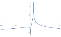
Figure 5. Graph of $B(z,tz)$ with the local maximum $t=-\frac{1}{\alpha-1}$ corresponding to the saddle point $v^{\ast}=-\frac{z}{\alpha-1}$. The level curve passing through $v^{\ast}$ contains two other points which are visible in this graph. They are obtained by intersecting the graph with the horizontal tangent at the latter local maximum. Their positions guarantee that the pole $z_{1}=0$ (which has a positive residue) is contained in the inner oval which implies that this level curve is of the non-relevant type shown in Fig. 4 c).

4.3. Convergence of the logarithmic potentials almost everywhere

By Cauchy’s integral formula (4.1), the monic polynomial $\tilde{\mathfrak{q}}_{n}$ which is proportional to the polynomial $\mathfrak{q}_{n}$ is given by

$$\tilde{\mathfrak{q}}_{n}(z):=\frac{(nd-([\alpha n]-1))!}{(nd)!}\mathfrak{q}_{n}(z)=\frac{([\alpha n]-1)!(nd-([\alpha n]-1))!}{2\pi i\cdot(nd)!}\int_{c}\frac{P^{n}(u)\,\mathop{}\!\mathrm{d}u}{(u-z)^{[\alpha n]}}.$$ (4.14)

The degree of the polynomial $\mathfrak{q}_{n}$ equals $d_{n}=nd-(m-1)$, where $m=[\alpha n]$. Recall that the logarithmic potential $L_{\mu_{n}}(z)$ of the root-counting measure $\mu_{n}$ of $\tilde{\mathfrak{q}}_{n}$ can be expressed as

$$L_{\mu_{n}}(z)=\frac{1}{d_{n}}\log|\tilde{\mathfrak{q}}_{n}(z)|.$$

By (4.2),

$$n=\frac{m}{\alpha}+s_{n},$$

where $0\leq s_{n}<1/\alpha$. Hence

$$d_{n}=\left(\frac{d-\alpha}{\alpha}\right)m+(s_{n}d+1)=\beta m+O(1),$$ (4.15)

where $\beta:=\frac{d-\alpha}{\alpha}$.

Lemma 4.10.

In the above notation,

$$\lim_{n\to\infty}\frac{1}{d_{n}}\log\left(\frac{(m-1)!(nd-(m-1))!}{(nd)!}\right)=\frac{\beta\log\beta-(\beta+1)\log(\beta+1)}{\beta}=:B.$$

Proof.

Straight-forward calculation using Stirling’s formula. ∎

Now we can calculate the limit of the sequence $\left\{\frac{1}{d_{n}}\log|\tilde{\mathfrak{q}}_{n}|\right\}$ of logarithmic potentials. Note that $d_{n}\sim\beta m$, take the logarithm of (4.14), and use Lemma 4.10 together with (4.13) in Corollary 4.8.

Corollary 4.11.

For any point $z\in\mathcal{O}$,

$$\lim_{n\to\infty}L_{\mu_{n}}(z)=B+\frac{1}{\alpha\beta}\left(\log|P(u^{\ast}_{max}(z))|-\alpha\log|u^{\ast}_{max}(z)-z|\right).$$

4.4. Convergence of $\{L_{\mu_{n}}\}_{n=1}^{\infty}$ in $L^{1}_{loc}$ and final steps of the proofs of Theorems 1.1 and 1.7

Corollary 4.11 provides the limit when $n\to\infty$ of the sequence $\{L_{\mu_{n}}\}$ a.e. in $\mathbb{C}$, but to settle Theorem 1.7 we need to prove that this limit also holds in $L^{1}_{loc}$. Vitali’s convergence theorem (see e.g. [Bo, Thm. 4.5.4 and Cor 4.5.5]) gives an appropriate criterion for this to hold. In our situation it provides the following corollary.

Lemma 4.12.

Let $\{p_{n}\}$ be a sequence of monic polynomials of strictly increasing degrees $d_{n}:=\deg p_{n}\to\infty$ as $n\to\infty$. Denote by $\mu_{n}:=\frac{1}{d_{n}}\sum_{i=1}^{d_{n}}\delta(\zeta_{i})$ the root-counting measure of $p_{n}$ and let $L_{n}(z):=\frac{1}{d_{n}}{\log|p_{n}(z)|}$ be the logarithmic potential of $\mu_{n}$. Assume that

1. there is a compact set $K\subset\mathbb{C}$ containing all the zeros $\zeta_{1},\dots,\zeta_{d_{n}}$ of $p_{n}$ for all $n=1,2,\dots$;

2. the sequence $\{L_{n}(z)\}$ converges to some locally integrable function $L(z)$ pointwise a.e. in $\mathbb{C}$.

Then, $L(z)$ is a $L^{1}_{loc}$-function and $\lim_{n\to\infty}L_{n}(z)=L(z)$ in the $L^{1}_{loc}$-sense.

Proof.

By Vitali’s convergence theorem, we only need to check the uniform integrability of our functions on an arbitrary fixed compact set $M\supset K$. Let $E$ be a set with Lebesgue measure $\lambda(E)<\epsilon<1$. Introduce

$$\log_{+}(x):=|\log|x||=f_{<\epsilon}(x)+f_{\geq\epsilon}(x),$$

where $f_{<\epsilon}(x)=\log_{+}(x)=-\log|x|$ if $0<x\leq\epsilon$, and $f_{<\epsilon}(x)=0$ if $x>\epsilon$. (Thus, $f_{\geq\epsilon}(x)=\log_{+}(x)$ if $x>\epsilon$, and $f_{\geq\epsilon}(x)=0$ if $0<x\leq\epsilon$).

We obtain

$$\int_{E}\left|L_{\mu_{n}}(z)\right|\,\mathop{}\!\mathrm{d}\lambda(z)\leq\frac{1}{d_{n}}\sum_{i=1}^{d_{n}}\int_{E}\log_{+}(z-\zeta_{i})\,\mathop{}\!\mathrm{d}\lambda(z)\leq$$ (4.16)

$$\leq\frac{1}{d_{n}}\sum_{i=1}^{d_{n}}\int_{E}f_{<\epsilon}(z-\zeta_{i})\,\mathop{}\!\mathrm{d}\lambda(z)+\frac{1}{d_{n}}\sum_{i=1}^{d_{n}}\int_{E}f_{\geq\epsilon}(z-\zeta_{i})\,\mathop{}\!\mathrm{d}\lambda(z):=I_{1}+I_{2}.$$ (4.17)

If $\mathbb{D}_{\epsilon}(\zeta_{i})$ is a disk of radius $\epsilon$ centered at $\zeta_{i}$, then

$$\int_{\mathbb{D}_{\epsilon}(\zeta_{i})}|\log|z-\zeta_{i}||\,\mathop{}\!\mathrm{d}z=-\pi\epsilon^{2}\left(\log\epsilon-\frac{1}{2}\right).$$ (4.18)

Hence

$$\int_{E}f_{<\epsilon}(z-\zeta_{i})\,\mathop{}\!\mathrm{d}\lambda(z)\leq\int_{\mathbb{D}_{\epsilon}(\zeta_{i})}f_{<\epsilon}(z-\zeta_{i})\,\mathop{}\!\mathrm{d}\lambda(z)=-\pi\epsilon^{2}\left(\log\epsilon-\frac{1}{2}\right)$$

which implies that

$$I_{1}\leq-\frac{1}{d_{n}}\left(d_{n}\pi\epsilon^{2}\left(\log\epsilon-\frac{1}{2}\right)\right)=O(\epsilon)$$

with a constant depending only on $\epsilon$. Let $\delta$ be the diameter of $M$. For the second sum in (4.17), let $m:=\max\{-\log\epsilon,\log_{+}(\delta)\}$ be the upper bound of $f_{\geq\epsilon}(x-\zeta)$ for $x,\zeta\in M$. Then $I_{2}\leq m\lambda(E)\leq m\epsilon=o(1)$ as $\epsilon\to 0$. The estimates for $I_{1}$ and $I_{2}$ and (4.16)-(4.18) prove that

$$\lim_{\lambda(E)\to 0}\underset{n}{\sup}\int_{E}|L_{n}(z)|\mathop{}\!\mathrm{d}\lambda(z)=0.$$

By Vitali’s theorem the desired convergence in $L^{1}_{loc}$ then follows from the convergence a.e., see e.g., [Bo, 4.5.2-4.5.5]. ∎

We now finalize our proof of Theorem 1.7. Observe that Corollary 4.11, reformulated in terms of the tropical trace, says that we have pointwise convergence a.e. provided by the formula

$$\lim_{n\to\infty}L_{\mu_{[\alpha n],n,P}}(z)=B+\tilde{\pi}_{*}H(z),$$

where $\tilde{\pi}:{U}_{rel}\to\mathbb{C}_{z}$ and $H(z,u)=\frac{1}{\beta}G(z,u)$. Together with Lemma 4.12 this fact implies that the sequence $\{L_{\mu_{[\alpha n],n,P}}(z)\}$ converges to the right-hand side of the latter formula in $L^{1}_{loc}$, and a fortiori is convergent as a sequence of distributions. This is the first part of Theorem 1.7. Since a measure $\mu_{\alpha,P}$ and its Cauchy transform are distributional derivatives of the logarithmic potential of $\mu_{\alpha,P}$, the other parts follow from the basic properties of distributions.

Next we will settle Theorem 1.1. The convergence $\mu_{n}\to\mu$ of Theorem 1.7 implies that $L_{\mu_{|\alpha n],n,P}}(z)\to L_{\mu_{\alpha,P}}(z)$ a.e. and hence

$$L_{\mu_{\alpha,P}}(z)=B+\tilde{\pi}_{*}H(z)$$

as $L^{1}_{loc}$-functions. Taking distributional derivatives gives for the Cauchy transform the relation

$$\mathcal{C}_{\mu_{\alpha,P}}=2\frac{\partial L_{\mu_{\alpha,P}}}{\partial z}=2\frac{\partial\tilde{\pi}_{*}H(z)}{\partial z}.$$

The distributional derivative of a continuous piecewise-harmonic subharmonic function is equal to its usual derivative a.e., see e.g. [BB, Prop. 2]. By Proposition 4.9, the tropical trace $\tilde{\pi}_{*}H(z)$ is such a function. Let us now calculate its derivative a.e. using the statement of Lemma 4.7 ii) saying that $\mathbb{C}$ can be covered a.e. by open sets $O_{i}\subset\mathcal{O},\ i\in I$, such that in each $O_{i}$ there is a branch $u=u^{\mathcal{D}}(z)$ of the saddle point curve $\mathcal{D}$ for which the equality

$$H(u^{\mathcal{D}}(z),z)=\tilde{\pi}_{*}H(z)$$ (4.19)

holds.

In other words, in each $O_{i}$ we get

$$2\beta^{-1}\frac{\partial G(z,u^{\mathcal{D}}(z))}{\partial z}=2\beta^{-1}\left(\frac{\partial G}{\partial z}(z,u^{\mathcal{D}}(z))+\frac{\partial G}{\partial u}(z,u^{\mathcal{D}}(z))\frac{\partial u^{\mathcal{D}}(z)}{\partial z}\right)=\mathcal{C}_{\mu_{\alpha,P}}(z).$$ (4.20)

The algebraic equation defining $\mathcal{D}$ (which is obviously satisfied by $u^{\mathcal{D}}$) says exactly that $\frac{\partial G}{\partial u}=0$. Hence

$$\beta^{-1}\frac{1}{u^{\mathcal{D}}-z}=\mathcal{C}_{\mu_{\alpha,P}}(z)\iff u^{\mathcal{D}}=z+(\beta\mathcal{C}_{\mu_{\alpha,P}}(z))^{-1}.$$

On the other hand, $u^{\mathcal{D}}$ satisfies equation (3.11), and therefore the Cauchy transform $\mathcal{C}=\mathcal{C}_{\mu_{\alpha,P}}$ satisfies a.e. in $\mathbb{C}$ the equation

$$(d-\alpha)\mathcal{C}=\frac{\mathop{}\!\mathrm{d}\left(\log{P}\left(z+(\beta\mathcal{C})^{-1}\right)\right)}{\mathop{}\!\mathrm{d}z}.$$ (4.21)

Formula (4.21) coincides with equation (1.4) which settles Theorem 1.1, up to a small shift of the order of the derivative. We have actually proven that the sequence of root-counting measures for $\{(P^{n})^{([\alpha n]-1)}\}$ converges, but using e.g., the main result of [To], we also get that the sequence considered in Theorem 1.1 has the same limit as that of $\{(P^{n})^{([\alpha n]-1)}\}$. ∎

4.5. The symbol curve $\Gamma$ is an instance of our general construction of affine Boutroux curves

Recall the general construction of an aBc in § 2.6. By following its steps we will see now that the symbol curve $\Gamma$ is a particular instance of this construction.

The starting point is the function

$$H(z,u):=\frac{1}{\beta}G(z,u):=\frac{1}{d-\alpha}(\log|P(u)|-\alpha\log|u-z|).$$

It is well-defined and pluriharmonic for all $(z,u)\in\mathbb{C}^{2}$ except at points where either $P(u)=0$ or $u=z$. Its differential is the meromorphic $1$-form given by

$$d(H(z,u)):=\frac{1}{2(d-\alpha)}\left(\frac{\alpha}{u-z}\mathop{}\!\mathrm{d}z+\left(\frac{P^{\prime}(u)}{P(u)}-\frac{\alpha}{u-z}\right)\mathop{}\!\mathrm{d}u\right).$$

The saddle point curve $\mathcal{D}\subset\mathbb{C}_{z}\times\mathbb{C}_{u}$ is the rational plane curve given by

$$2(d-\alpha)\frac{\partial H}{\partial u}=\frac{P^{\prime}(u)}{P(u)}-\frac{\alpha}{u-z}=0.$$

Restricting $H$ to $\mathcal{D}$, we get a simplified expression for its differential given by

$$dH(z,u)=\frac{1}{2\beta}\cdot\frac{1}{u-z}\,\mathop{}\!\mathrm{d}z,\quad(z,u)\in\mathcal{D}.$$

Consider the usual projection $\pi:\mathcal{D}\to\mathbb{C}_{z}$ sending $(z,u)$ to $z$. Except for a finite number of branch points, $z$ is a local coordinate on $\mathcal{D}$. Since $\mathcal{D}$ is smooth by Corollary 3.9, in a neighborhood of every point $p=(z,u)\in\mathcal{D}$, the restriction of $H$ to $\mathcal{D}$ is a real-valued harmonic function satisfying

$$H(p)-H(p_{0})=\text{Re }\int_{p_{0}}^{p}\frac{1}{\beta(u-z)}\,\mathop{}\!\mathrm{d}z,$$

where $p_{0}$ is another fixed point on $\mathcal{D}$. In particular, this implies that the form

$$\omega=\frac{\mathop{}\!\mathrm{d}z}{\beta(u-z)}\,$$

has imaginary periods on $\mathcal{D}$ which also follows from Theorem 3.3. Notice that $\mathcal{D}$ is not an aBc, but if we change coordinates as explained below the resulting curve will become an aBc.

Namely, the affine curve $\mathcal{E}$ introduced in § 2.6 is constructed from the differential of $H$ as $\mathrm{Spec}\ \mathbb{C}[z,\frac{1}{\beta(u-z)}]$. In our case this step just corresponds to the change of coordinates

$$v=\frac{1}{\beta(u-z)},\ z=z\quad\iff\quad u=z+\frac{1}{\beta v},\;z=z.$$

Hence, for the above pluriharmonic function $H$, the Boutroux curve $\mathcal{E}$ given in § 2.6 is precisely the symbol curve $\Gamma$ defined by equation (1.3) and is satisfied by the asymptotic Cauchy transform $\mathcal{C}_{\mu_{\alpha,P}}$ according to Theorem 1.1.

5. Differential equations satisfied by Rodrigues’ descendants

5.1. Deriving the differential equations

In this section we obtain linear differential equations satisfied by the Rodrigues’ descendants and use them to deduce equations  (1.4) and  (1.3) independently of most of the machinery in this paper, given a few additional assumptions. Having in mind future applications and generalisations, we derive a differential equation for the Rodrigues’ descendants not just for a polynomial $P$, but for a more general meromorphic function of the form

$$f(z):=P(z)e^{T(z)}/Q(z),$$

where $P(z)\not\equiv 0,\,Q(z)\not\equiv 0$ and $T(z)$ are polynomials with $\gcd(P,Q)=1$. In case $T\equiv 0$ and $Q\equiv 1$, we have $f(z)=P(z)$ considered in the present paper, see Corollary 5.3.

Proposition 5.1.

In the above notation and for $d:=\deg{P}+\deg{Q}+\deg{T}$, the Rodrigues’ descendant $\mathcal{R}_{m,n,Pe^{T}/Q}(z)$ satisfies the linear homogeneous differential equation

$$\begin{split}&\sum_{i=0}^{d}\sum_{j=0}^{i}\sum_{k=0}^{j}\frac{(m+d-i+n(2j-i))\delta_{k,0}-nkT^{(k)}}{(m+d-i)!(i-j)!(j-k)!k!}P^{(i-j)}Q^{(j-k)}y^{(d-i)}=0\end{split}$$ (5.1)

of order $d$. Here $\delta_{k,0}=\begin{cases}1,\text{if}\;k=0\\ 0,\;\text{otherwise.}\end{cases}$

As special cases of the latter statement we obtain the following three corollaries.

Corollary 5.2.

The Rodrigues’ descendant $\mathcal{R}_{m,n,P/Q}(z)$ of a rational function $P(z)/Q(z)$ satisfies the linear homogeneous differential equation

$$\sum_{i=0}^{d}\sum_{j=0}^{i}\frac{m+d+(n-1)i-2nj}{(m+d-i)!\,(i-j)!\,j!}P^{(j)}Q^{(i-j)}y^{(d-i)}=0$$ (5.2)

of order $d=\deg{P}+\deg{Q}$.

Corollary 5.3.

The Rodrigues’ descendant $\mathcal{R}_{m,n,P}(z)$ of a polynomial $P(z)$ satisfies the linear homogeneous differential equation

$$\sum_{i=0}^{d}\frac{(m-nd)-(i-d)(n+1)}{(d+m-i)!\,i!}P^{(i)}y^{(d-i)}=0$$ (5.3)

of order $d=\deg{P}$.

Remark 5.4.

Differential equations satisfied by $\frac{\mathrm{d}^{m}}{\mathrm{d}z^{m}}\left(Q_{1}^{N_{1}}Q_{2}^{N_{2}}\dotsm Q_{d}^{N_{d}}\right)$, where $Q_{1},\dotsc,Q_{d}$ are polynomials in $z$ and $N_{1},\dots,N_{d}$ are nonnegative integers, were previously derived by Ciorânescu (see [Ci]). As Ciorânescu remarks, one of these differential equations looks strikingly similar to Pochhammer’s generalized Gaussian differential equation. A special case was later rediscovered by J. M. Horner (see [Ho]).

The original Rodrigues’ formula inspires the following consequence of Corollary 5.3.

Corollary 5.5.

The Rodrigues’ descendant $y=\mathcal{R}_{n,n,P}(z):=\frac{\mathop{}\!\mathrm{d}^{n}}{\mathop{}\!\mathrm{d}z^{n}}(P^{n}(z))$ satisfies the linear differential equation

$$\sum_{i=0}^{d}\frac{(d-1)-(i-1)(n+1)}{(d+n-i)!\,i!}P^{(i)}y^{(d-i)}=0$$ (5.4)

of order $d=\deg{P}$.

Proof of Proposition 5.1.

Consider the first-order differential equation

$$PQw^{\prime}+n(PQ^{\prime}-P^{\prime}Q-PQT^{\prime})w=0,$$ (5.5)

Clearly, if $f=Pe^{T}/Q$, then $w=f^{n}$ satisfies (5.5). By differentiating both sides of (5.5) $\ell\geq d-1$ times (or $\ell>d-1$ times if $d=0$) and using Leibniz’s rule for the derivative of a product, we get

$$\sum_{i=0}^{\ell}\binom{\ell}{i}U^{(i)}w^{(\ell+1-i)}+n\cdot\sum_{i=0}^{\ell}\binom{\ell}{i}V^{(i)}w^{(\ell-i)}-n\cdot\sum_{i=0}^{\ell}\binom{\ell}{i}W^{(i)}w^{(\ell-i)}=0,$$ (5.6)

where $U:=PQ,\,V:=PQ^{\prime}-P^{\prime}Q$ and $W:=PQT^{\prime}$. In the first sum, remove the first term and replace $i$ by $r+1$ in the remaining sum. In the second and third sums, replace $i$ by $r$ and remove the last terms. By combining the three resulting sums and simplifying, equation (5.6) becomes

$$Uw^{(\ell+1)}+nV^{(\ell)}w-nW^{(\ell)}w+\sum_{r=0}^{\ell-1}\binom{\ell}{r}\left(\frac{\ell-r}{r+1}U^{(r+1)}+nV^{(r)}-nW^{(r)}\right)w^{(\ell-r)}=0.$$ (5.7)

By changing the upper limit of summation in (5.7) from $\ell-1$ to $\ell$, the terms $nV^{(\ell)}w$ and $-nW^{(\ell)}w$ are encompassed by the sum. Since $U,\,V$ and $W$ are polynomials of degrees at most $d,\,d-1$ and $d-1$, respectively and $\ell\geq d-1$, we can change the upper limit of summation further to $d-1$, since higher terms vanish. That is, we obtain the equation

$$Uw^{(\ell+1)}+\sum_{r=0}^{d-1}\binom{\ell}{r}\left(\frac{\ell-r}{r+1}U^{(r+1)}+nV^{(r)}-nW^{(r)}\right)w^{(\ell-r)}=0,$$

or equivalently, if we replace $r$ by $i-1$, change the lower index of summation to $i=0$, and define $0\cdot V^{(-1)}=0\cdot W^{(-1)}=0$ as to not introduce any new terms,

$$\sum_{i=0}^{d}\frac{\ell!}{(\ell-i+1)!\,i!}\left((\ell-i+1)U^{(i)}+niV^{(i-1)}-niW^{(i-1)}\right)w^{(\ell-i+1)}=0.$$ (5.8)

Since the terms in $U$ and $V$ contain two factors, while $W$ contains three factors, we expand their derivatives using Leibniz’s rule as follows:

$$U^{(i)}=(P\cdot Q\cdot 1)^{(i)}=PQ^{(i)}+\sum_{j=0}^{i-1}\sum_{k=0}^{j}\binom{i}{i-j,j-k,k}P^{(i-j)}Q^{(j-k)}\delta_{k,0},$$ (5.9)

$$\begin{split}V^{(i-1)}&=(P\cdot Q^{\prime}\cdot 1)^{(i-1)}-(P^{\prime}\cdot Q\cdot 1)^{(i-1)}\\ &=\sum_{j=0}^{i-1}\sum_{k=0}^{j}\binom{i-1}{i-j-1,j-k,k}\left(P^{(i-j-1)}Q^{(j-k+1)}-P^{(i-j)}Q^{(j-k)}\right)\delta_{k,0},\end{split}$$ (5.10)

$$W^{(i-1)}=(P\cdot Q\cdot T^{\prime})^{(i-1)}=\sum_{j=0}^{i-1}\sum_{k=0}^{j}\binom{i-1}{i-j-1,j-k,k}P^{(i-j-1)}Q^{(j-k)}T^{(k+1)}.$$ (5.11)

By inserting the expressions in (5.9)-(5.11) into (5.8) and simplifying, we see that

$$\begin{split}&\sum_{i=0}^{d}\binom{\ell}{i}PQ^{(i)}w^{(\ell-i+1)}+\sum_{i=0}^{d}\sum_{j=0}^{i-1}\sum_{k=0}^{j}\frac{\ell!}{(\ell-i+1)!(i-j)!(j-k)!k!}\left[(\ell-i+1)P^{(i-j)}Q^{(j-k)}\delta_{k,0}\right.\\ &+\left.n(i-j)\left(\left(P^{(i-j-1)}Q^{(j-k+1)}-P^{(i-j)}Q^{(j-k)}\right)\delta_{k,0}-P^{(i-j-1)}Q^{(j-k)}T^{(k+1)}\right)\right]w^{(\ell-i+1)}=0.\end{split}$$ (5.12)

By changing the upper index of summation from $i-1$ to $i$ in (5.12), and using the convention that $0\cdot P^{(-1)}=0$ as previously, the first sum is encompassed by the triple sum. Next, reverse the order of summation in the outer sum, and let $m:=\ell-d+1$, which gives that

$$\begin{split}&\sum_{i=0}^{d}\sum_{j=0}^{d-i}\sum_{k=0}^{j}\frac{(m+d-1)!}{(m+i)!(d-i-j)!(j-k)!k!}\left[(m+i)P^{(d-i-j)}Q^{(j-k)}\delta_{k,0}+n(d-i-j)\times\right.\\ &\left.\left(\left(P^{(d-i-j-1)}Q^{(j-k+1)}-P^{(d-i-j)}Q^{(j-k)}\right)\delta_{k,0}-P^{(d-i-j-1)}Q^{(j-k)}T^{(k+1)}\right)\right]w^{(m+i)}=0,\end{split}$$ (5.13)

for all $\ell=m+d-1\geq d-1\iff m\geq 0$. Now let $(\ast)$ denote the equation obtained by replacing $w^{(m+i)}$ by $y^{(i)}$ in (5.13). Clearly, $y=w^{(m)}=(f^{n})^{(m)}=((Pe^{T}/Q)^{n})^{(m)}$ satisfies $(\ast)$. Thus, by reversing the order of summation in $(\ast)$ and simplifying, the proposition follows. ∎

Corollaries 5.2, 5.3, and  5.5 are immediate consequences of Proposition 5.1.

5.2. An algorithm for obtaining an algebraic equation satisfied by the asymptotic Cauchy transform $\mathcal{C}$

In § 4.4 we proved that the Cauchy transform of the asymptotic root-counting measure $\mu_{\alpha,P}$ satisfies the algebraic equations (1.4) and  (1.3). We will now see that this also follows formally from equation  (5.3), using a scheme suggested in [BBS]. (It is observed that the formal derivation is validated under the assumption that hypotheses i) - iii) of Proposition 3 in loc. cit. hold.)

In the notation of § 1 our algorithm is as follows:

Step 1: Multiply both sides of equation  (5.3) by the constant $(m+d-1)!$ (which we retained in the proof of Proposition  5.1 until the final simplification).

Step 2: Replace $m$ by $\alpha n$ and divide both sides by $y$.

Step 3: Replace $y^{(d-i)}/y$ by $(n(d-\alpha)\mathcal{C})^{d-i}$ in the resulting equation and divide both sides by $n^{d}$.

Step 4: Let $n\to\infty$.

By carrying out the above four steps, the resulting equation becomes

$$\sum_{i=0}^{d}\frac{\alpha^{i-1}(\alpha-i)(d-\alpha)^{d-i}}{i!}P^{(i)}(z)\mathcal{C}^{d-i}=0$$ (5.14)

which is identical to equation  (1.4) up to the choice of the index of summation. As previously, using the scaled Cauchy transform $\mathcal{W}=\frac{d-\alpha}{\alpha}\mathcal{C}$ we can transform equation  (5.14) into

$$\sum_{i=0}^{d}\frac{\alpha-i}{i!}P^{(i)}(z)\mathcal{W}^{d-i}=0.$$ (5.15)

Since $P(z+u)=\sum_{i=0}^{d}\frac{P^{(i)}(z)}{i!}u^{i}$ and $uP^{\prime}(z+u)=\sum_{i=0}^{d}i\frac{P^{(i)}(z)}{i!}u^{i}$ (which can be seen from the Taylor expansions of the left-hand sides of these equations around $u=0$), we can use the change of variable $u=1/\mathcal{W}$ along with these two sums to transform equation  (5.15) into

$$\alpha P(z+\mathcal{W}^{-1})-\mathcal{W}^{-1}P^{\prime}(z+\mathcal{W}^{-1})=0.$$ (5.16)

Notice that if $z=b$ is a multiple zero of $P$, then $\mathcal{W}=(b-z)^{-1}$ solves equation  (5.16) and consequently such $\mathcal{W}$ also solve equation  (5.15). Finally, equation  (5.16) is easily rewritten in the form

$$\alpha\mathcal{W}=\frac{P^{\prime}\left(z+\mathcal{W}^{-1}\right)}{P\left(z+\mathcal{W}^{-1}\right)}=\frac{\mathop{}\!\mathrm{d}\log{P}(z+\mathcal{W}^{-1})}{\mathop{}\!\mathrm{d}z}.$$ (5.17)

which can be transformed back into equation  (1.3).

It should also be noted that the above algorithm can be used with the differential equation  (5.1) in Proposition  5.1 as its starting point. From this procedure, it is possible to derive the algebraic equation

$$\alpha\mathcal{W}=\frac{\mathop{}\!\mathrm{d}\log{f}(z+\mathcal{W}^{-1})}{\mathop{}\!\mathrm{d}z}$$ (5.18)

where $f(z)=P(z)e^{T(z)}/Q(z)$ is the meromorphic function defined in the beginning of this section and $\mathcal{W}$ is the scaled Cauchy transform of the asymptotic root-counting measure associated with $\mathcal{R}_{[\alpha n],n,Pe^{T}/Q}(z)$. This procedure (which involves slightly more elaborate Taylor expansions of functions such as $P(z+u)Q(z+u),\,u\cdot\frac{\partial}{\partial u}(P(z+u)Q(z+u))$ and $u\cdot Q(z+u)\cdot\frac{\partial}{\partial u}P(z+u)$) strongly suggests that the main results of this paper can be generalized to Rodrigues’ descendants of such functions $f$.

6. Case of a quadratic polynomial $P(z)$

The simplest instance of our study occurs when $P$ is a quadratic polynomial. This case is closely related to the Legendre polynomials and the original Rodrigues’ formula. For these polynomials, the asymptotic behavior of their zeros is known since long. In particular, for $\alpha=1$, the density of the asymptotic root distribution of the polynomials (1.1) equals

$$\eta(x)=\frac{1}{\pi}\frac{1}{\sqrt{1-x^{2}}}\mathop{}\!\mathrm{d}x,\;x\in[-1,1].$$

For general $\alpha$, the asymptotic measure has been recently calculated by Hoskins and Kabluchko [HoKa], by using methods quite different from ours. (Paper [HoKa] refers to a draft version of the present text.)

In order to illustrate our methods, we will explicitly calculate the asymptotic measure $\mu_{\alpha,P}$ for qudratic $P$. Without loss of generality, we can assume that $P(z)=z^{2}-1$ and $0<\alpha<2$, and consider the polynomial sequence

$$P_{n}^{(\alpha)}(x):=\frac{\mathop{}\!\mathrm{d}^{[\alpha n]}(x^{2}-1)^{n}}{\mathop{}\!\mathrm{d}x^{[\alpha n]}}.$$

By the Gauss-Lucas theorem, the zeros of these polynomials are contained in the interval $[-1,1]$, but we will not use this fact directly taking instead a more circuitous route via the saddle-point analysis suggested in the previous sections.

For $P(z)=z^{2}-1$, the saddle point curve $\mathcal{D}\subset\mathbb{C}_{z}\times\mathbb{C}_{u}$ defined in the previous section gives

$$P^{\prime}(u)(u-z)=\alpha P(u)\iff(2-\alpha)u^{2}-2uz+\alpha=0.$$

The projection $\pi:\mathcal{D}\to\mathbb{C}_{z}$ has two branch points $b_{\pm}=\pm\sqrt{\alpha(2-\alpha)}$. Since $0<\alpha<2$, both branch points are real. The curve $\mathcal{D}$ has two branches:

$$u_{\pm}(z)=\frac{1}{2-\alpha}(z\pm\sqrt{z^{2}+\alpha^{2}-2\alpha}).$$

The monodromy along a contour that encircles both branch points is trivial, so the two branches are well defined in $V:=\mathbb{C}\setminus[b_{-},b_{+}]$. Let $u_{\pm}(z)$ be the branch that satisfies $u_{\pm}(z)=\frac{1}{2-\alpha}(z\pm\sqrt{z^{2}+\alpha^{2}-2\alpha})$ on the interval $I_{\alpha}:=[b_{+},\infty[$ of the positive real axis.

By Corollary 3.9, we know that there is one branch which goes to $\infty$ as $|z|\to\infty$. This branch is clearly $u_{+}$. By the same corollary, the other branch $u_{-}$ goes to the root of $P^{\prime}(u)=0$ which in our case is $u=0$.

On the negative real axis the branch that goes to infinity as $|z|\to\infty$ will be given by $u_{+}(z)=\frac{1}{2-\alpha}(z-\sqrt{z^{2}+\alpha^{2}-2\alpha})$, and hence the identity

$$u_{+}(-z)=-u_{+}(z)$$ (6.1)

holds everywhere, since it holds on a non-discrete set.

The pluriharmonic function given by (1.7) equals

$$H(z,u)=\frac{1}{2-\alpha}\left(\log|u^{2}-1|-\alpha\log|u-z|\right).$$ (6.2)

For $u\in\mathcal{D}$, we get

$$H(z,u)=\frac{1}{2-\alpha}\left(\log\left(\frac{2}{\alpha}\right)+\log|u|+(1-\alpha)\log|u-z|\right).$$ (6.3)

Set $H_{\pm}(z):=H(u_{\pm}(z),z)$ and notice that (except at the poles) $H_{\pm}(z)$ are harmonic functions well-defined in $V=\mathbb{C}\setminus[b_{-},b_{+}]$ and enjoy the following properties.

Lemma 6.1.

i) $H_{+}(-z)=H_{+}(z)$.

ii) $H_{+}$ can be extended to a continuous piecewise-harmonic function in $\mathbb{C}$, possibly with singularities at $\pm 1$.

iii) If $0<\alpha<1$, $H_{+}(z)$ has two poles at $z=\pm 1$ with the asymptotic near these poles given by $H_{+}(z)\sim\frac{1-\alpha}{2-\alpha}\cdot\mathrm{log}|z\mp 1|$.

iv) If $1\leq\alpha<2$, $H_{+}(z)$ has no poles.

Proof.

Item i) follows from the relation $H(-u,-z)=H(z,u)$ together with (6.1). To settle ii), notice that if $z\in[b_{-},b_{+}]$, then $\sqrt{z^{2}-b_{\pm}^{2}}$ is purely imaginary providing that $|u_{-}(z)|=|u_{+}(z)|$ and $|u_{-}(z)-z|=|u_{+}(z)-z|$. This implies that $H_{+}(z)=H_{-}(z)$. Since the monodromy around the branch points will interchange $u_{-}(z)$ and $u_{+}(z)$, $H_{+}(z)$ is continuous for $z\in]b_{-},b_{+}[$. Hence it is continuous except possibly at $\pm 1$.

To prove iii) and iv), observe that for $\alpha=1$, equation (6.3) shows that $H_{+}(z)$ has no pole at $z=\pm 1$. If $\alpha\neq 1$ the Taylor expansion of $u_{+}(z)$ at $z=1$ gives

$$u_{+}(z)=\frac{1+|\alpha-1|}{2-\alpha}+\frac{|\alpha-1|+1}{|\alpha-1|(2-\alpha)}(z-1)+O(z-1)^{2}.$$ (6.4)

For $1<\alpha<2$, (6.4) implies that $u_{+}(1)=\frac{\alpha}{2-\alpha}$ and, in particular, both $u_{+}(1)$ and $u_{+}(1)-1$ are non-zero. Using (6.3) and i), we obtain iv). If $0<\alpha<1$, then (6.4) simplifies to

$$u_{+}(z)=1+\frac{(z-1)}{1-\alpha}+O(z-1)^{2}.$$ (6.5)

Thus $\log|u_{+}(z)-z|\sim\log|z-1|$ near $z=1$. Again using (6.3) and i) we obtain iii). ∎

The level curve $\Delta:H_{+}(z)=H_{-}(z)$ and its complement $\mathcal{O}$ are shown in Fig. 6. (Recall that by Lemma 4.2, we get that $\mathcal{O}$ is open and dense in $\mathbb{C}$ for an arbitrary strongly generic polynomial $P$. For $P=z^{2}-1$, this fact is obvious directly. If $\alpha\neq 1$, then $\gamma$ consists of two ovals centered around $\pm 1$ together with the interval $[b_{-},b_{+}]$ of the real axis. For $\alpha=1$, $\gamma$ is simply the interval $[-1,1]$.

The additional circumstance which simplifies the application of our results in the case of quadratic $P$ is that the set $U_{max}$ of maximally relevant saddle points has an easy description which we will now provide. Set $W_{+}=\{(z,u_{+}(z)),\quad z\in O\}$ and recall that $\pi:\mathbb{C}^{2}\to\mathbb{C}$ is the standard projection sending $(z,u)$ to $z$.

Figure 6. The curve $\Delta$ given by $H_{+}(z)=H_{-}(z)$. The piecewise behavior of $\pi_{*}H(z)$ in the connected components of $\mathcal{O}=\mathbb{C}\setminus\Delta$ is marked in each such component, while $\tilde{\pi}_{*}H(z)$ equals $H_{+}(z)$ in all the components.

The above figure and the next proposition also describe the relevant saddle points, as a presheaf $F$ on $\mathcal{O}$, in the way that was explicated at the end of § 2.3. Namely, over the complement of the two finite components of $\mathcal{O}$ each stalk consists of the two points in the fiber of $\pi$, while the stalk over the two components consists of the only point $(s,u_{+}(z))$.

Proposition 6.2.

In the above notation, we get

$${U_{max}}\cap\pi^{-1}O=W_{+}.$$

Note that the tropical trace $\tilde{\pi}_{*}H(z)$ for the map $\tilde{\pi}:U_{rel}\to\mathbb{C}_{z}$ equals the tropical trace for the restriction $\tilde{\pi}:U_{max}\to\mathbb{C}_{z}.$ Hence, our earlier results and Proposition 6.2 easily provide the asymptotic behavior of the zeros of the Rodrigues descendants of $P(z)=z^{2}-1$. For fixed $0<\alpha<2$, let $\mu_{n}:=\mu_{|\alpha n],n,P}$ be the root-counting measure of $\mathcal{R}_{[\alpha n],n,P}=(P^{n})^{([\alpha n])}(z)$ with logarithmic potential $L_{\mu_{n}}(z)$ and Cauchy transform $\mathcal{C}_{\mu_{n}}(z)$. (Note the very explicit description of $\tilde{\pi}_{*}H(z)$ in item i) below.)

Corollary 6.3.

1. The equality

   $$\lim_{n\to\infty}L_{\mu_{n}}(z)=\tilde{\pi}_{*}H(z)+B=H_{+}(z)+B,$$

   is valid in the $L^{1}_{loc}$-sense, where $H(z,u)$ is given by (6.2) and the constant $B$ is defined in Lemma 4.10 with $d=2$.

2. For $0\leq\alpha<1$, one has

   $$\mu:=\mu_{\alpha,P}:=\lim_{n\to\infty}\mu_{n}=\frac{2}{\pi}\frac{\partial^{2}H_{+}}{\partial z\partial\bar{z}}.$$

   The measure $\mu$ is the probability measure explicitly given by

   $$\mu=\frac{1}{(2-\alpha)\pi}\frac{\sqrt{b_{+}^{2}-x^{2}}}{1-x^{2}}\mathop{}\!\mathrm{d}s+\frac{1-\alpha}{2-\alpha}\delta(1)+\frac{1-\alpha}{2-\alpha}\delta(-1),\quad x\in[b_{-},b_{+}],$$

   and its continuous part is supported on $[b_{-},b_{+}]$.

3. For $1\leq\alpha<2$, one has

   $$\mu:=\lim_{n\to\infty}\mu_{n}=\frac{2}{\pi}\frac{\partial^{2}H_{+}}{\partial z\partial\bar{z}}.$$

   Here $\mu$ is the probability measure explicitly given by

   $$\mu=\frac{1}{(2-\alpha)\pi}\frac{\sqrt{b_{+}^{2}-x^{2}}}{1-x^{2}}\mathop{}\!\mathrm{d}s,\quad x\in[b_{-},b_{+}].$$

4. The Cauchy transform $\mathcal{C}_{\mu}(z)=\frac{2\partial L_{\mu}}{\partial z}$ is the analytic continuation of the function

   $$\mathcal{C}_{\mu}(x)=\frac{2\alpha}{(\alpha-1)x+\sqrt{x^{2}-b_{+}^{2}}},\quad x\in]1,\infty]$$

   to the domain $\mathbb{C}\setminus[b_{-},b_{+}]$.

   It satisfies equation (5.16) which in our special case reduces to

   $$\alpha P\left(z+\frac{\alpha}{2-\alpha}\mathcal{C}^{-1}\right)-\frac{\alpha}{2-\alpha}\mathcal{C}^{-1}P^{\prime}\left(z+\frac{\alpha}{2-\alpha}\mathcal{C}^{-1}\right)=0\iff$$

   $$\frac{\alpha}{2-\alpha}+\frac{2(1-\alpha)}{2-\alpha}z\mathcal{C}+(1-z^{2})\mathcal{C}^{2}=0.$$

Remark 6.4.

The above items ii) and iii) have previously been derived by Hoskins and Kabluchko in [HoKa, 4.2]. As was pointed to us by an anonymous referee item iii) in particular is known in the literature as the Kesten-McKay law, see [DuEd].

Proof.

The previous proposition implies that the fiberwise maximum on $U_{max}$ in the definition of $\tilde{\pi}_{*}H(z)$ is taken just on the single sheet $W_{+},$ and hence $\tilde{\pi}_{*}H(z)=H_{+}(z)$ as $L^{1}_{loc}$-functions. Theorem 1.7 then gives i).

Since by Lemma 6.1, $\tilde{\pi}_{*}H(z)$ is continuous and harmonic a.e. in $\mathbb{C}$ its distributional derivative equals its derivative a.e., see e.g. [BB, Prop.2]. Hence

$$\mathcal{C}_{\mu}(z)=2\frac{\partial L_{\mu}}{\partial z}=\frac{2}{2-\alpha}\left(\frac{u_{+}^{\prime}(z)}{u_{+}(z)}+\frac{u_{+}^{\prime}(z)-1}{u_{+}(z)-z}\right),$$

which can be reduced to iv).

By the Plemelj-Sokhotski formula, the distributional derivative $\frac{\partial\mathcal{C}_{\mu}}{\partial\bar{z}}$ along $[b_{-},b_{+}]$ equals one half of the absolute value of the jump of the function across the line segment $[b_{-},b_{+}]$, i.e., $\frac{|C_{+}-C_{-}|}{2}$, where $C_{+}$ och $C_{-}$ are the two values of the analytic continuation of $\mathcal{C}_{\mu}$ on both sides of $[b_{-},b_{+}]$, see e.g. [BB, Lemma 2]. This fact explains the expressions for the continuous part of the measure in ii) and iii). For $0<\alpha<1$, the point mass contributions are immediate from Lemma 6.1 iii). The equation for the Cauchy transform follows from Theorem 1.1 and (4.21). ∎

The description of $\tilde{\pi}_{*}H(z)=H_{+}(z)$ in Corollary 6.3 can be contrasted with the behavior of the fiberwise maximum $\pi_{*}H(z)$. In each of the three regions determined by $\Delta$, $\pi_{*}H(z)$ equals the maximum of $H_{-}$ and $H_{+}$. It is also clear that $\pi_{*}H(z)=H_{+}(z)$ for large $|z|$, and hence in the whole unbounded region. Inside the ovals $H_{-}(z)$ will be the larger function, and hence $\pi_{*}H(z)=H_{-}(z)$. Thus $\pi_{*}H(z)$ is the piecewise-harmonic function shown in Fig. 6. By an argument similar to the proof of Lemma 6.1, $H_{-}(z)$ has no poles when $0<\alpha<1$, and so $\pi_{*}H(z)$ is subharmonic in the whole plane. On the other hand, if $1<\alpha<2$, $H_{-}(z)$ has poles at $z=\pm 1$ and near these poles $H_{-}(z)\sim\frac{1-\alpha}{2-\alpha}\log|z\mp 1|$ respectively. So $\pi_{*}H(z)$ is subharmonic only in the complement of the poles.

Proof of Proposition 6.2.

By Lemma 4.4 for each $z\in\mathcal{O}$, there is a unique maximally relevant saddle point. Thus we only need to show that this saddle point is not $u_{-}(z)$. By Lemma 4.7, a change of the branch that determines the maximally relevant saddle point can only occur when $z$ moves to a different connected component of $\mathcal{O}$. Consequently, it suffices to analyse the saddle point behavior of $H(z,u^{\ast})$ for some points $z$ in each connected component of $\mathcal{O}$, say, on the real axis.

The left-right symmetry induced by $H(-z,-u)=H(z,u)$ and $u_{\pm}(-z)=-u_{\pm}(z)$ shows that the level curves through $u_{\pm}(-z)$ and $u_{\pm}(z)$ are the mirror images of each other. Hence, by the definition of maximally relevant saddle points, it is enough to consider a real point $z_{1}$ inside the right oval, in addition to a real point $z_{2}$ outside both ovals, i.e., in the unbounded component.

Observe that for a saddle point $w(z)$ not to be maximally relevant, it suffices that the two paths $\gamma_{i},$ $i=1,2,$ of maximal growth from $w(z)$ have the same pole as their endpoints; see Remark 4.5. Note that such an endpoint can only coincide with $P^{+}$, $\infty$ or $u_{\pm}(z)$, all of which belong to the real axis if $z\geq b_{+}$.

For $z$ real, we have the additional symmetry $H(z,\bar{u})=H(z,u)$ which implies the following:

i) each level set of $H(z,u)$ in the complex $u$-plane passing through a saddle point on the real axis is invariant under the complex conjugation;

ii) the gradient field of $H(z,u)$ in the complex $u$-plane is invariant under complex conjugation w.r.t. the variable $u$.

In particular, ii) implies that if the oriented paths $\gamma_{i},\ i=1,2,$ starting at the real saddle point $u_{-}(z)\in\mathbb{R}$, do not initially follow the real axis, they will have the same endpoint which necessarily belongs to the real axis. This endpoint has three possibilities; it can either be $P^{+}$, $\infty$, or $u_{+}(z)$. In the first two cases, $u_{-}(z)$ is not maximally relevant, by Remark 4.5. In the latter case $u_{-}(z)$ will be relevant, but not maximally relevant. This follows from the fact that in order for a maximally relevant saddle point to exist, the two paths of maximal growth from $u_{+}(z)$ must have different endpoints $P^{+}$ and $\infty$. Hence $u_{+}(z)$ is maximally relevant. Thus we have established that $u_{+}(z)$ is maximally relevant in all three cases under the assumption that $\gamma_{i},\ i=1,2$, do not initially follow the real axis. Let us finally show that our latter assumption holds, i.e., indeed $\gamma_{i},\ i=1,2$, do not initially follow the real axis.

A simple computation gives

$$\frac{\mathop{}\!\mathrm{d}H(z,t)}{\mathop{}\!\mathrm{d}t}=\frac{(t-u_{-}(z))(t-u_{+}(z))}{(2-\alpha)(t^{2}-1)(t-z)}.$$ (6.6)

Now if $z\geq 0$ is large, then $u_{+}(z)\geq 0$ will also be large while $u_{-}(z)$ will be close to $0$. Hence, for $t$ close to $u_{-}(z)$, the sign of $\frac{\mathop{}\!\mathrm{d}H(z,t)}{\mathop{}\!\mathrm{d}t}$ will be equal to the sign of $-(t-u_{-}(z))$, which implies that $u_{-}(z)$ is a local maximum of $H(z,t)$, $t\in\mathbb{R}$. In particular, the paths of maximal growth cannot start out along the real axis implying that $u_{-}(z)$ is not maximally relevant. If $z$ is contained in the oval in the right half-plane, we have that $u_{-}(z)<u_{+}(z)$ and we can assume that for $\alpha\neq 1$, $z<1$. A straightforward calculation shows that if $1<\alpha<d$, we get $z<1<u_{-}(z)<u_{+}(z)$, and if $0<\alpha<1$, then $u_{-}(z)<u_{+}(z)<z<1$. Analyzing signs in (6.6) we again conclude that $u_{-}(z)$ is a local maximum of $H(z,t)$ for real $t$. The result follows. ∎

A more instructive illustration of why $u_{+}(z)$ is a maximally relevant saddle point is given by Fig. 7 – 8 which show the level curves passing through both saddle points.

Let us start with the case $0<\alpha<1$ presented in Fig. 7. The dashed line is the level curve of $H(z,u)$ through $u_{+}(z)$ and we see from its definition and the location of the poles that $u_{+}(z)$ is a maximally relevant saddle point. There exists a path of maximal ascent going from $u_{+}(z)$ to $P^{+}$ and another one going from $u_{+}(z)$ first to $u_{-}(z)$ and then to $\infty$. The non-dashed curve is the level curve of $H(z,u)$ through $u_{-}(z)$. We can conclude that this saddle point is non-relevant, either by definition, or since it is impossible to reach $P^{+}$ by an ascending path from $u_{-}(z)$. Hence the only maximally relevant saddle point is $u_{+}(z)$ and inside the right oval we get $\tilde{\pi}_{*}H(z)=H(z,u_{1}(z))=H_{+}(z)$ as was already proven before.

For $1\leq\alpha<2$, the level curves look differently, see Fig. 8. But again it is possible to use the position of the poles and the definition of maximally relevant saddle points to obtain the same result.

Figure 7. The level curves of $H(z,u)$ through the saddle points, $0<\alpha<1$. (Here $\alpha=0.2$ and $z=0.615$.)

Let us now qualitatively describe what happens to $\mu_{\alpha,z^{2}-1}$ when $\alpha$ increases from $0$ to $2$. Part of the mass of the two point measures at $\pm 1$ initially moves out of $\pm 1$ to the continuous measure supported on the interval $I_{\alpha}:=[b_{-},b_{+}]$. The latter measure then expands with increasing $\alpha$, until its support becomes the whole interval $[-1,1]$ at $\alpha=1$. Then when $1<\alpha<2$ there is no mass left at $\pm 1$ and the support of the continuous measure shrinks toward the origin and vanishes when $\alpha=2$. In particular, for all $0<\alpha<2$, the support of the asymptotic measure is contained in $[-1,1]$, as predicted by the Gauss-Lucas theorem, and for all $\alpha\neq 1$, it is (except for the possible point masses) strictly smaller than $[-1,1]$.

To summarize: we want to find $\tilde{\pi}_{*}H(z)$ to obtain the asymptotic root-counting measure. By considering the complement $\mathcal{O}$ of the non-simple locus $\Delta$, it suffices to check the situation in the finite number of connected components of $\mathcal{O}$, see Proposition 2.10. Furthermore, in each such component it is enough to analyze the behavior of the paths of maximal ascent at a single point. In principle, such analysis can be carried out for higher degree polynomials $P$ as well, but is substantially more involved.

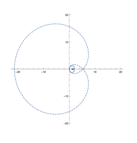
Figure 8. The level curves of $H(z,u)$ through the saddle points, $1<\alpha<2$. (Here $\alpha=1.2$ and $z=0.615$.)

7. Final remarks and open problems

1. Practically all the results of the present paper can be generalized to the case where $f$ is a rational function instead of a polynomial. However poles of a rational function restrict the possibility of deformation of the integration contour used in § 5 which leads to a more delicate situation requiring special analysis.

2. The set-up of the present paper can also be randomized and generalized as follows. Let $\xi$ be a probability measure compactly supported in $\mathbb{C}$. Denote by $P_{n}=\prod_{i=1}^{n}(x-\xi_{i})$ a random polynomial of degree $n$ whose roots are i.i.d. random variables sampled on $\xi$. Given a sequence $\mathcal{A}=\{\alpha_{n}\}$ of non-negative integers, set $Q_{n}=P_{n}^{(\alpha_{n})}$ and denote by $\mu_{n}$ the root-counting measure of $Q_{n}$. Results from the recent papers [PeRi, Ka] motivate the following guess.

Conjecture 7.1.

In the above notation, the following two statements hold:

(i) if $\frac{\alpha_{n}}{n}\to 0$, then the sequence $\{\mu_{n}\}$ converges in probability to $\xi;$

(ii) if $\frac{\alpha_{n}}{n}\to\alpha,\;0<\alpha<1$, then the sequence $\{\mu_{n}\}$ converges in probability to a measure $\xi_{\alpha}$ whose support is contained in the convex hull of the support of $\xi$;

Results of the present paper can be interpreted in the above terms as follows. We start with a discrete probability measure $\xi$ assigning the mass $\frac{1}{d}$ to each of the $d$ zeros of $P(z)$. Then we sample this measure uniformly and deterministically $nd$ times, by forming the sequence of polynomials $\{P_{n}(z):=P^{n}(z)\}$. Finally, fixing $0<\alpha<\deg P$, we differentiate each $P_{n}(z)$ $[n\alpha]$ times. This procedure creates a sequence of polynomials $\{Q_{n}(z)\}$ and an associated sequence of root-counting measures $\{\mu_{n}\}$. The proportion between the number of derivations and the number of sampled points has the limit

$$A:=\frac{\alpha}{d}.$$

Observe now that $\frac{1}{d}\log|P(z)|$ equals the logarithmic potential $L_{\xi}(z)$ of the above measure $\xi$. Therefore our presentation of the asymptotic measure in Theorem 1.7 can be interpreted as

$$\lim_{n\to\infty}\mu_{n}=\frac{2}{\pi}\frac{\partial^{2}}{\partial z\partial\bar{z}}\tilde{\pi}_{*}\left(\frac{1}{1-A}L_{\xi}(w)-\frac{A}{1-A}\log|w-z|\right),$$ (7.1)

where $\tilde{\pi}_{*}$ denotes the fiberwise maximum of the function

$$H(z,w):=\frac{1}{1-A}L_{\xi}(w)-\frac{A}{1-A}\log|w-z|$$

considered on the open subset $U_{max}\subset\mathcal{D}$ of maximally relevant saddle points on the curve

$$\mathcal{D}=\{(z,w)\in\mathbb{C}_{z}\times\mathbb{C}_{w}\;|\;\frac{\partial H(z,w)}{\partial w}=0\},$$

where

$$2\frac{\partial H(z,w)}{\partial w}=\frac{1}{1-A}\mathcal{C}_{\xi}(w)-\left(\frac{A}{1-A}\right)\frac{1}{w-z}=0\iff\mathcal{C}_{\xi}(w)=\frac{A}{z-w}.$$

Observe now that the right-hand side of formula (7.1) depends on the measure $\xi$ and does not explicitly use the underlying polynomial $P$. Hence one can hope that (7.1) might make sense for an arbitrary probability measure $\xi$ where a random polynomial sequence $\{Q_{n}(z)\}$ is obtained by independent sampling of roots according to $\xi$. At least, it seems plausible that the relation (7.1) holds for a much more general class of probability measures $\xi$ than the very special measure originating from a univariate polynomial $P$ which we described above and which implicitly appears in our paper.

3. For a given strongly generic polynomial $P$ and $0<\alpha<\deg P$, the asymptotic root-counting measure $\mu_{\alpha,P}=\lim_{n\to\infty}\mu_{[\alpha n],n,P}$ defined in § 1 is supported inside a certain intriguing domain $\Upsilon_{P}\subset\mathbb{C}$ which we call the shadow of a polynomial $P$; see examples in Fig.  2 where $\Upsilon_{P}$ is shown in red. Further, we say that a polynomial $P$ of degree at least $3$ has roots in convex position if each of them lies on the boundary of $\mathrm{Conv}_{P}$, where $\mathrm{Conv}_{P}$ denotes their convex hull.

Conjecture 7.2.

For any strongly generic polynomial $P$ of degree at least $3$ whose roots are in convex position, but do not form a regular polygon, one has

(i) $\Upsilon_{P}\subset\mathrm{Conv}_{P}$ is a concave domain, i.e., the boundary of $\Upsilon_{P}$ consists of a finite number of smooth curves $\gamma_{k},\,k=1,\dots,\eta$, such that the interior of the line segment connecting any two distinct points on $\gamma_{k}$ lies entirely in the complement of $\Upsilon_{P}$.

(ii) The boundary of $\Upsilon_{P}$ is contained in the union over $\alpha\in[0,d]$ of all critical values w.r.t. the variable $z$ of the rational function

$$F_{\alpha}(z)=z-\alpha\frac{P(z)}{P^{\prime}(z)}.$$ (7.2)

Equivalently, the boundary of $\Upsilon_{P}$ consists of all values of $u$ for which the family

$$\Phi(\alpha,z,u)=\alpha P(z)+(u-z)P^{\prime}(z)$$

has a multiple root w.r.t. $z$ for some fixed $\alpha\in[0,d]$.

Curiously, the function $F_{\alpha}(z)$ in (7.2) bears a strong resemblance with the iterated expression in the relaxed Newton’s method, see e.g. [Su]. Additionally, the family $\Phi(\alpha,z,u)$ is a natural generalization of the polar derivative $dP(z)+(u-z)P^{\prime}(z)$ of $P$ with pole $u$, see e.g. [Ma]. (Also compare this family to the polynomial appearing after the relation (4.10) above). Finally, if the parameter $\alpha$ runs over the whole real line, the union of all critical values of (7.2) appears to form $d-1$ hyperbola-like branches in $\mathbb{C}$ that interact with $\Upsilon_{P}$.

4. Let $P$ be a cubic strongly generic polynomial with non-collinear zeros, and let $h=h(\mathcal{W})$ denote the left-hand side of equation (3.2). If we solve the quartic equation $\mathrm{Resultant}(h,h^{\prime})/P=0$ in $z$ for $\alpha=0,1,3$, the twelve solutions that arise are various triangle centers associated with the triangle $T_{P}$ in $\mathbb{C}$ whose vertices are the roots of $P$. The distinct among these twelve points are: the center of mass of $T_{P}$, the roots of $P$ and $P^{\prime}$, the first and second isodynamic points of $T_{P}$ (denoted by $\mathcal{I}_{1}$ and $\mathcal{I}_{2}$, respectively), and an additional point that we denote $\mathcal{A}$. (Here $\mathcal{A}$ is the point $X(26613)$ in the Encyclopedia of Triangle Centers, see [Ki, HSS].) Numerical experiments indicate that the support of the asymptotic root-counting measure $\mu_{1,P}$ (in the notation of Theorem 1.1) has non-obvious connections to some of these points, and is either a tree with three edges that have a vertex in common, or two disjoint edges; see Fig. 9.

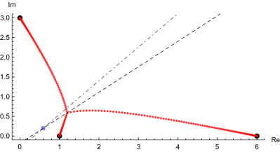
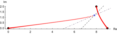
Figure 9. The zeros of $\mathcal{R}_{100,100,P}(z)$ (shown by small red dots). Here, the square is the branch point $\mathcal{A}$, and the two lines are $\overline{A\mathcal{I}_{1}}$ and $\overline{A\mathcal{I}_{2}}$, respectively. Note that one of the two lines seems to always pass through the vertex of degree 3 in the tree formed by the support of $\mu_{1,P}$ whenever it exists.

More generally, our numerical experiments support the following guess.

Conjecture 7.3.

In the notation of Theorem 1.1, for $0<\alpha<\deg P$, the support of $\mu_{\alpha,P}$ is an embedded graph in $\mathbb{C}$ without cycles, i.e., it is a forest.

5. The Rodrigues descendants $\mathcal{R}_{n,n,P}(z)$ satisfy multiple orthogonal conditions in the following sense.

Lemma 7.4.

Assume that $P(z)=(z-z_{1})\dotsm(z-z_{d})$ has only simple roots and let $\gamma$ be a path connecting $z_{i}$ and $z_{j}$, $1\leq i<j\leq d$. Then

$$I:=\int_{\gamma}z^{k}\,\mathcal{R}_{n,n,P}(z)\,\mathop{}\!\mathrm{d}z=0$$ (7.3)

where $k=0,1,\dots,n-1$.

Proof.

Follows from integration by parts $n$ times. ∎

Taking $d-1$ homologically non-equivalent different paths $\gamma_{1},\gamma_{2},\dots,\gamma_{d-1}$ among paths connecting the roots of $P$ leads to the multiple orthogonality conditions. For $d>2$, the sequence $\{\mathcal{R}_{n,n,P}(z)\}$ itself does not satisfy any linear recurrence of finite length. On the other hand, fixing a system $\gamma_{1},\gamma_{2},\dots,\gamma_{d-1}$ of paths as above, one can introduce the family of (type II) multiple orthogonal polynomials indexed by $\mathbf{n}=(n_{1},n_{2},\dots,n_{d-1})$ where the polynomial $\mathcal{R}_{\mathbf{n}}(z)$ has degree $n_{1}+n_{2}+\dots+n_{d-1}$ and satisfies the system of orthogonality relations given by

$$\int_{\gamma_{j}}z^{k_{j}}\,\mathcal{R}_{\mathbf{n}}(z)\,\mathop{}\!\mathrm{d}z=0,\;k_{j}=0,1,\dots,n_{j}-1\;\text{and}\;j=1,2,\dots,d-1.$$

(One can check that the above system determines $\mathcal{R}_{\mathbf{n}}(z)$ up to a scalar factor). Obviously, $\mathcal{R}_{n,n,P}(z)$ are the special cases of more general polynomials $\mathcal{R}_{\mathbf{n}}(z)$ corresponding to $\mathbf{n}=(n,n,\dots,n)$. The multi-indexed family $\{\mathcal{R}_{\mathbf{n}}(z)\}$ satisfies a finite recurrence relation of length $d+1$, see [VA].

6. Our final remark concerns Theorem 2.23.

Conjecture 7.5.

Under the assumptions of Theorem 2.23 the signed measure whose existence is proven in this result is unique.

References

- [AbSt] M. Abramowitz, I. A. Stegun, Handbook of mathematical functions with formulas, graphs, and mathematical tables. National Bureau of Standards Applied Mathematics Series, 55, Washington, D.C. 1964 xiv+1046 pp.
- [Al] S. Altmann, Olinde Rodrigues, mathematician and social reformer. Gazeta de matemática, Janeiro (2007), n 152.
- [AlOr] S. Altman, E. L. Ortiz (eds), Mathematics and social utopias in France. Olinde Rodrigues and his times. History of Mathematics, vol. 28, (2005), xi+168 pages.
- [As] R. Askey, “The 1839 paper on permutations: its relation to the Rodrigues formula and further developments”, in S. Altmann, E.L. Ortiz (eds). Mathematics and Social Utopias in France: Olinde Rodrigues and His Times, History of Mathematics, vol. 28, p. 105. American Mathematical Society, Providence (2005).
- [BaSh] Y. Baryshnikov, B. Shapiro, Quadratic differentials and signed measures, Journal d’Analyse Mathématique, DOI: 10.1007/s11854-021-0158-3.
- [Be] M. Bertola, Boutroux curves with external field: equilibrium measures without a variational problem, Anal. Math. Phys. (2011) 1:167–211.
- [BM] M. Bertola, M. Y. Mo, Commuting difference operators, spinor bundles and the asymptotics of orthogonal polynomials with respect to varying complex weights. Adv. Math. 220(1), (2009), 154–218.
- [BBB] J.-E. Björk, J. Borcea, R.Bøgvad, Subharmonic Configurations and Algebraic Cauchy Transforms of Probability Measures. Notions of Positivity and the Geometry of Polynomials Trends in Mathematics (2011) 39–62.
- [Bi] N. Bleistein, Mathematical methods for wave phenomena, Academic Press, Orlando, 1984.
- [Bo] V. I. Bogachev. Measure theory. Vol. I, II. Springer-Verlag, Berlin 2007.
- [BB] J. Borcea, R. Bøgvad, Piecewise harmonic subharmonic functions and positive Cauchy transforms Pacific J. Math 240 (2009) 231-265.
- [BBS] R. Bøgvad, J.Borcea, B. Shapiro, Homogenized spectral problems for exactly solvable operators: asymptotics of polynomial eigenfunctions Publ. Res. Inst. Math. Sci., vol. 45, (2009) 525–568.
- [BoSh] R. Bøgvad, B. Shapiro, On mother body measures with algebraic Cauchy transform. L’Enseignement Math., vol. 62, (2016) 117–142.
- [Br] N. G. De. Bruijn, Asymptotic methods in analysis, North-Holland Publishing Co., Amsterdam, 1961.
- [Ci] N. Ciorânescu, Sur une nouvelle généralisation des polynomes de Legendre. Acta Math. 61, 135–148 (1933). https://doi.org/10.1007/BF02547789
- [DuEd] A. Dubbs, A. Edelman, Infinite random matrix theory, tridiagonal bordered toeplitz matrices, and the moment problem, Linear Algebra and its Applications, vol. 467, (2015), 188–201.
- [Fe] H. Federer, Geometric measure theory, Die Grundlehren der mathematischen Wissenschaften, Band 153 Springer-Verlag New York Inc., New York 1969 xiv+676 pp.
- [Ga] J. B. Garnett, Analytic capacity and measure, LNM 297, Springer-Verlag, 1972, 138 pp.
- [GrHa] P. Griffiths, J. Harris, Principles of algebraic geometry. Reprint of the 1978 original. Wiley Classics Library. John Wiley & Sons, Inc., New York, (1994) xiv+813 pp.
- [GrKr] S. Grushevsky, I. Krichever, The universal Whitham hierarchy and the geometry of the moduli space of pointed Riemann surfaces, Surveys in differential geometry. Vol. XIV. Geometry of Riemann surfaces and their moduli spaces, 111–129, Surv. Differ. Geom., 14, Int. Press, Somerville, MA, 2009.
- [HoKa] J. Hoskins, Z. Kabluchko, Dynamics of zeroes under repeated differentiation, arXiv:2010.14320.
- [Ho] J. M. Horner, Generalized Rodrigues formula solutions for certain linear differential equations. Tr. AMS (1965) 31–42.
- [HSS] C. Hägg, B. Shapiro, M. Shapiro, Introducing isodynamic points for binary forms and their ratios, arXiv:2207.01658.
- [Ka] Z. Kabluchko, Critical points of random polynomials with independently identically distributed roots. Proc. AMS, Volume 143, Number 2, February (2015) 695–702.
- [KiTa] A. Kiselev, Ch. Tan, The flow of polynomial roots under differentiation, arXiv: 2012.09080.
- [Ki] C. Kimberling, Encyclopedia of Triangle Centers. http://faculty.evansville.edu/ ck6/encyclopedia
- [Ma] M. Marden, Geometry of Polynomials, 2nd ed., Math. Surverys 3, Amer. Math. Soc. Providence, RI, 1966.
- [MaJo] M. Johansson, I grund och botten, Albert Bonniers Förlag, Stockholm, 1956.
- [Os] C. O’Sullivan, Revisiting the saddle point method of Perron, Pacific J. Math., Vol. 298, No. 1, 2019.
- [PeRi] R. Pemantle, I. Rivin, The distribution of zeros of the derivative of a random polynomial. In I. Kotsireas and E. V. Zima, editors, Springer, New York, 2013.
- [Ra] T. Ransford, Potential theory in the complex plane. Cambridge University Press, 1995, 232 pp.
- [STT] B. Shapiro, K. Takemura, M. Tater, On spectral polynomials of the Heun equation. II, Comm. Math. Phys. vol 311, issue 2 (2012), 277–300.
- [St1] S. Steinerberger, Conservation Laws for the Density of Roots of Polynomials under Differentiation, arXiv:2001.09967.
- [St2] S. Steinerberger, A Nonlocal Transport Equation Describing Roots of Polynomials Under Differentiation, arXiv:1811.04844.
- [Su] S. Sutherland, Bad Polynomials for Newton’s Method. In Linear and Complex Analysis, Springer-Verlag (1994).
- [To] V. Totik, The Gauss-Lucas theorem in an asymptotic sense. Bull. Lond. Math. Soc. 48 (2016), no. 5, 848–854.
- [VA] W. Van Assche, Nearest neighbor recurrence relations for multiple orthogonal polynomials. J. Approx. Theory 163(10), 1427–1448 (2011).