Physical conditions in the warped accretion disk of a massive star

Young massive stars warm up the large amount of gas and dust which condenses in their vicinity, exciting a forest of lines from different molecular species. Their line brightness is a diagnostic tool of the gas physical conditions locally, which we use to set constraints on the environment where massive stars form. We made use of the Atacama Large Millimeter/submillimeter Array at frequencies near 349 GHz, with an angular resolution of $0\aas@@fstack{\prime\prime}1$, to observe the methyl cyanide (CH₃CN) emission which arises from the accretion disk of a young massive star. We sample the disk midplane with twelve distinct beams, where we get an independent measure of the gas (and dust) physical conditions. The accretion disk extends above the midplane showing a double-armed spiral morphology projected onto the plane of the sky, which we sample with ten additional beams: along these apparent spiral features, gas undergoes velocity gradients of about 1 km s^-1 per 2000 au. The gas temperature (T) rises symmetrically along each side of the disk, from about 98 K at 3000 au to 289 K at 250 au, following a power law with radius, R^-0.43. The CH₃CN column density (N) increases from 9.2 $\times$ 10¹⁵ cm^-2 to 8.7 $\times$ 10¹⁷ cm^-2 at the same radii, following a power law with radius, R^-1.8. In the framework of a circular gaseous disk observed approximately edge-on, we infer an H₂ volume density in excess of 4.8 $\times$ $10^{9}$ cm^-3 at a distance of 250 au from the star. We study the disk stability against fragmentation following the methodology by Kratter et al. (2010), appropriate under rapid accretion, and we show that the disk is marginally prone to fragmentation along its whole extent.

1 Introduction

The circumstellar regions within a few 1000 au from early-type young stars, where the (average) kinetic temperature of the interstellar medium exceeds 100 K, are rich in methyl cyanide gas (CH₃CN), whose relative abundance with respect to H₂ is typically larger than 10^-9 (e.g., Hernández-Hernández et al. 2014). CH₃CN is a symmetric top molecule whose millimeter spectrum is divided into groups of rotational transitions, with the following favourable properties (e.g., Boucher et al. 1980; Loren & Mundy 1984): (i) each group corresponds to a single $J\to(J-1)$ transition with varying $K$, where $J$ and $K$ are the two quantum numbers of total angular momentum and its projection on the axis of molecular symmetry, respectively; (ii) each group of transitions covers a “narrow” bandwidth, within about a GHz, and is separated by a few tens of GHz from the lower and higher $J$ transitions; (iii) the energy levels within a group are only populated through collisions, and their excitation temperatures span many 100 K; (iv) rotational transitions of the isotopologue CH${}_{3}^{13}$CN emit within the same narrow bandwidth of the CH₃CN transitions with same quantum numbers. These spectral properties make of CH₃CN emission a sensitive thermometer for the interstellar gas, where the H₂ density exceeds a critical value of approximately $10^{5}$ cm^-3 (e.g., Shirley 2015); this critical density would be reached, for instance, inside a spherical core of 0.1 pc radius (R), gas mass of 50 M_⊙, and density proportional to $\rm R^{-1.5}$.

Since the first CH₃CN interferometric observations by Cesaroni et al. (1994), performed with the Plateau de Bure Interferometer at 110 GHz, CH₃CN emission and its isotopologue CH${}_{3}^{13}$CN have been observed at (sub-)arcsecond resolution towards tens of early-type young stars, in order to estimate the linewidth, temperature, and H₂ number density of local gas (e.g., Zhang et al. 1998; Beltrán et al. 2005; Beuther et al. 2005; Chen et al. 2006; Qiu et al. 2011; Hernández-Hernández et al. 2014; Hunter et al. 2014; Sánchez-Monge et al. 2014; Zinchenko et al. 2015; Bonfand et al. 2017; Ilee et al. 2018; Ahmadi et al. 2018; Johnston et al. 2020). For instance, CH₃CN ($12_{K}$–$11_{K}$) observations at 220 GHz, whose lower excitation energy (E${}_{l}/k$) exceeds 58 K, indicate average rotational (and kinetic) temperatures of 200 K approximately, and CH₃CN column densities of the order of 10¹⁶ cm^-2. These conditions are met at radii of 1000 au from the brightness peak of the dust continuum emission at the same frequency, whose position is assumed to pinpoint a young star. Alternatively, temperature and density gradients measured through CH₃CN transitions are proxies for the radiative feedback of luminous stars in the making ($>$ $10^{3}$ L_⊙).

Table 1: Summary of ALMA observations at Cycle 4 (project code 2016.1.01200.S).

Array Conf.	R.A. (J2000)	Dec. (J2000)	VLSR	Freq. Cove.	$\Delta\nu$	BP Cal.	Phase Cal.	Pol. Cal.	HPBW
	(h m s)	(∘ ′ ′′)	(km s-1)	(GHz)	(kHz)				(′′)
(1)	(2)	(3)	(4)	(5)	(6)	(7)	(8)	(9)	(10)
C40–6	18:34:40.290	–09:00:38.30	77.4	335.6, 349.6	976.5	J1751$+$0939	J1825$-$0737	J1733$-$1304	0.10

In this paper, we report on spectroscopic CH₃CN, CH₃OH (methanol), and dust continuum observations with the Atacama Large Millimeter/submillimeter Array (ALMA) at 349 GHz with an angular resolution of $0\aas@@fstack{\prime\prime}1$. We exploit the CH₃CN ($19_{K}$–$18_{K}$) K-ladder, with excitation energies ranging from 168 K (for K $=$ 0) to 881 K (for K $=$ 10), to probe, at different radii, the physical conditions in the accretion disk of an early-type young star. We targeted the star-forming region G023.01$-$00.41, at a trigonometric distance of 4.59${}^{+0.38}_{-0.33}$ kpc from the Sun (Brunthaler et al. 2009), where we recently revealed the accretion disk around a young star of $10^{4.6}$ L_⊙, corresponding to a ZAMS star of 20 M_⊙ (Sanna et al. 2019, their Fig. 1); the disk was imaged by means of spectroscopic ALMA observations of both CH₃CN and CH₃OH lines at $0\aas@@fstack{\prime\prime}2$ resolution in the 230 GHz band. The disk extends up to radii of 3000 au from the central star where it warps above the midplane; here, we resolve the outer disk regions in two apparent spirals projected onto the plane of the sky. We showed that molecular gas is falling in and slowly rotating with sub-Keplerian velocities down to radii of 500 au from the central star, where we measured a mass infall rate of $6\times 10^{-4}$ M_⊙ yr^-1 (Sanna et al. 2019, their Fig. 5). The disk and star system drives a radio continuum jet and a molecular outflow aligned along a position angle of $57\degr$, measured east of north (Sanna et al. 2016, their Fig. 2); their projected axis is oriented perpendicular to the disk midplane whose inclination with respect to the line-of-sight was estimated to be less than $30\degr$ (namely, the disk is seen approximately edge-on; Sanna et al. 2014, 2019). Previously, we also measured the average gas conditions over the same extent of the whole disk, by means of Submillimeter Array (SMA) observations of the CH₃CN ($12_{K}$–$11_{K}$) emission, and estimated a kinetic temperature of 195 K and CH₃CN column density of $5.1\times 10^{16}$ cm^-2 (Sanna et al. 2014, their Fig. 2 and Table 4).

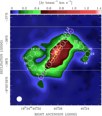
Figure 1: Spatial morphology of dense gas around the most massive star (star symbol) in G023.01$-$00.41: moment-zero map of the CH₃OH ($14_{1,13}$–$14_{0,14}$) A⁺ emission (colors). The upper wedge quantifies the line intensity from its peak to the maximum negative in the map; black contours are drawn at levels of 10, 50, and 100 times the 1 $\sigma$ rms of 2.8 mJy beam^-1 km s^-1. The disk plane, with white ticks at steps of 500 au, is drawn from the central star position at a position angle of $-33\degr$ (see Sect. 3). The synthesized ALMA beam is shown in the bottom left corner. White empty circles mark areas (hereafter, “pointings”) where the CH₃CN spectra of Figs. 8 and 9 are integrated and are labeled from 1 to 22 (cf. column 1 of Table 2).

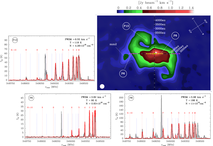
Figure 2: Physical conditions in the accretion disk of G023.01$-$00.41. Main panel: same image (and symbols) as in Fig. 1, with the equatorial reference system (top right) rotated clockwise by $57^{\circ}$, in order to align the (projected) outflow direction with the vertical axis of the plot. For three selected pointings indicated in white, we plot the local integrated spectra at 349 GHz in the side panels (grey histograms), as an example of the molecular line profiles and fitting. The cluster source “mm2” is marked; this source might alter the accretion disk around the primary (star symbol). Side panels: examples of different CH₃CN ($19_{K}$–$18_{K}$) spectra extracted in the inner (P8), outer (P6), and apparent spiral regions (P13) of the accretion disk (identifier on the top left). Positions of CH₃CN and CH${}_{3}^{13}$CN components are labeled in red and blue, respectively, with K ranging from 0 up to 10. The brightest line at a rest frequency of 349.107 GHz corresponds to the CH₃OH emission imaged in the main panel; this line shows a bright maser contribution in the inner-region spectra (e.g., P8). Red profiles draw the synthetic spectra fitted with MCWeeds by Monte Carlo Markov chains method assuming LTE; best fit parameters of intrisic FWHM, excitation temperature, and column density of CH₃CN are listed on the top right (cf. Table 2). We note that the excess of emission visible in the higher K lines of the observed spectrum at position P8, with respect to the synthetic spectrum, is likely due to contamination from different molecular species.

2 Observations and calibration

We observed the star-forming region G023.01$-$00.41 with the 12 m-array of ALMA in band 7 (275–373 GHz). Observations were conducted under program 2016.1.01200.S on 2017 July 10 (Cycle 4) during a 3 hour run, with precipitable water vapor of 0.35–0.38 mm. The 12 m-array observed with 40 antennas covering a baseline range between 16 m and 2647 m, achieving an angular resolution and maximum recoverable scale of approximately $0\aas@@fstack{\prime\prime}08$ and $1\aas@@fstack{\prime\prime}4$, respectively. Observation information is summarized in Table 1.

We made use of a mixed correlator setup consisting of four basebands (BB1–4), three operated in time division mode (TDM) and one in frequency division mode (FDM). Each TDM window had 64 spectral channels spaced over a bandwidth of 1875 MHz. These bands were used for continuum (full) polarization observations and tuned at the central frequencies of 336.57 (BB1), 338.57 (BB2), and 348.57 GHz (BB3) for optimal polarization performance (cf. ALMA Cycle 4 Proposer’s Guide, Doc 4.2. ver. 1.0, March 2016). The FDM window had 1920 spectral channels spaced over a bandwidth of 938 MHz, to achieve a velocity resolution of 0.84 km s^-1 after spectral averaging by a factor of 2. This band was used for spectral line observations and tuned at the central frequency of 349.15 GHz (BB4), and overlaps with the higher half of BB3. BB4 was placed to cover the K-ladder of the CH₃CN ($19_{K}$–$18_{K}$) transition, with K ranging from 0 to 10, and its isotopologue CH${}_{3}^{13}$CN.

In the following, we report on the analysis of the high spectral-resolution band (BB4); the targeted molecular lines are listed in Table 3 of the Appendix, and include a bright CH₃OH line previously identified in a preparatory SMA experiment (project code 2014B-S006). The visibility data were calibrated with the Common Astronomy Software Applications (CASA) package, version 4.7.2 (r39762), making use of the calibration scripts provided with the quality assessment process (QA2). To determine the continuum level, we made use of the spectral image cube and selected the line-free channels from a spectrum integrated over a circular area of $0\aas@@fstack{\prime\prime}5$ in size, which was centered on the target source. The task uvcontsub of CASA was used to subtract a constant continuum level across the spectral window (fitorder $=$ 0). We imaged the line and continuum emission with the task clean of CASA setting a circular restoring beam size of $0\aas@@fstack{\prime\prime}114$, equal to the geometrical average of the major and minor axes of the beam obtained with a Briggs’s robustness parameter of 0.5. We achieve a sensitivity of approximately 1 mJy beam^-1 per resolution unit, which corresponds to a brightness temperature of about 1 K over a beam of $0\aas@@fstack{\prime\prime}1$. The continuum emission was integrated over a line free bandwidth of 52 MHz achieving a sensitivity of 0.2 mJy beam^-1.

Table 2: Physical parameters of the CH₃CN gas and dust observed near 349 GHz towards the accretion disk in G023.01$-$00.41.

ID	X-offset	Y-offset	Rp	Sdust	voff	FWHMint	Trot	N${}_{\rm CH_{3}CN}$	size	$\tau_{4}$	M500	N${}_{\rm H_{2}}$
	(′′)	(′′)	(au)	(mJy)	(km s-1)	(km s-1)	(K)	(1016 cm-2)	(mas)		(M⊙)	(1023 cm-2)
(1)	(2)	(3)	(4)	(5)	(6)	(7)	(8)	(9)	(10)	(11)	(12)	(13)
Eastern disk side
P1	–0.074	–0.056	250	29.7	+0.78$\pm$0.03	7.37$\pm$0.20	$267^{+2}_{-2}$	$56.75^{+0.53}_{-0.58}$	70	9.64	0.16	10.0
P2	–0.015	–0.147	750	13.6	+3.25$\pm$0.03	5.17$\pm$0.56	$197^{+2}_{-2}$	$35.80^{+0.80}_{-0.73}$	95	15.00	0.10	6.2
P3	+0.045	–0.238	1250	4.6	+2.69$\pm$0.03	4.79$\pm$0.16	$140^{+3}_{-2}$	$9.33^{+0.33}_{-0.31}$	95	6.31	0.05	2.9
P4	+0.104	–0.330	1750	3.8	+2.83$\pm$0.03	3.09$\pm$0.09	$118^{+3}_{-2}$	$6.17^{+0.30}_{-0.27}$	90	7.01	0.05	2.9
P5	+0.163	–0.421	2250	2.8	+1.86$\pm$0.07	3.94$\pm$0.06	$110^{+7}_{-7}$	$1.41^{+0.20}_{-0.17}$	100	1.27	0.04	2.3
P6	+0.223	–0.512	2750	2.9	+1.70$\pm$0.04	3.82$\pm$0.07	$90^{+5}_{-5}$	$0.83^{+0.07}_{-0.07}$	100	0.75	0.05	2.9
Western disk side
P7	–0.133	+0.036	250	34.2	–0.56$\pm$0.03	7.12$\pm$0.13	$279^{+2}_{-2}$	$40.92^{+0.43}_{-0.37}$	70	6.53	0.17	11.1
P8	–0.193	+0.127	750	14.7	–0.20$\pm$0.03	5.98$\pm$0.10	$198^{+3}_{-3}$	$11.01^{+0.27}_{-0.27}$	95	4.00	0.11	6.6
P9	–0.252	+0.218	1250	6.7	+0.07$\pm$0.03	5.82$\pm$0.17	$153^{+3}_{-3}$	$8.31^{+0.20}_{-0.28}$	95	4.33	0.06	3.9
P10	–0.311	+0.310	1750	4.8	+1.07$\pm$0.05	4.54$\pm$0.07	$129^{+6}_{-5}$	$3.39^{+0.30}_{-0.25}$	90	2.53	0.05	3.3
P11	–0.371	+0.401	2250	3.6	+1.56$\pm$0.07	3.54$\pm$0.10	$120^{+10}_{-10}$	$0.87^{+0.18}_{-0.23}$	100	0.86	0.04	2.7
P12	–0.430	+0.492	2750	2.8	+1.88$\pm$0.06	2.72$\pm$0.11	$100^{+10}_{-10}$	$0.25^{+0.03}_{-0.02}$	65	0.33	0.04	2.6
Northeastern apparent spiral
P13	+0.293	+0.003	1822	3.0	+1.33$\pm$0.05	6.55$\pm$0.16	$119^{+4}_{-3}$	$4.26^{+0.26}_{-0.28}$	114	2.28	0.04	2.3
P14	+0.408	–0.002	2349	3.2	+1.22$\pm$0.04	5.43$\pm$0.11	$119^{+4}_{-4}$	$3.55^{+0.22}_{-0.23}$	114	2.28	0.04	2.4
P15	+0.468	–0.100	2656	3.0	+1.15$\pm$0.06	6.78$\pm$0.10	$116^{+5}_{-4}$	$2.69^{+0.23}_{-0.17}$	114	1.40	0.04	2.3
P16	+0.445	–0.215	2689	3.6	+0.57$\pm$0.07	6.66$\pm$0.14	$107^{+5}_{-4}$	$3.89^{+0.39}_{-0.33}$	90	2.09	0.05	3.1
P17	+0.380	–0.310	2613	3.6	+1.24$\pm$0.06	4.69$\pm$0.15	$102^{+4}_{-3}$	$4.27^{+0.37}_{-0.32}$	90	3.25	0.05	3.2
Southwestern apparent spiral
P18	–0.754	–0.110	3020	$<$ 0.6	+0.57$\pm$0.08	8.58$\pm$0.15	$115^{+6}_{-6}$	$2.29^{+0.23}_{-0.17}$	90	0.94	0.01	0.5
P19	–0.800	–0.007	3196	$<$ 0.6	+1.56$\pm$0.09	11.51$\pm$0.18	$110^{+15}_{-12}$	$0.69^{+0.26}_{-0.12}$	90	0.21	0.01	0.5
P20	–0.752	+0.098	3017	$<$ 0.6	+0.81$\pm$0.09	6.95$\pm$0.13	$90^{+15}_{-15}$	$0.32^{+0.34}_{-0.12}$	90	0.16	0.01	0.6
P21	–0.651	+0.152	2620	$<$ 0.6	+0.77$\pm$0.10	6.66$\pm$0.08	$110^{+10}_{-13}$	$0.60^{+0.20}_{-0.11}$	90	0.32	0.01	0.5
P22	–0.540	+0.178	2181	0.8	+0.35$\pm$0.08	5.90$\pm$0.08	$121^{+10}_{-9}$	$1.07^{+0.28}_{-0.22}$	90	0.63	0.01	0.6

3 Results

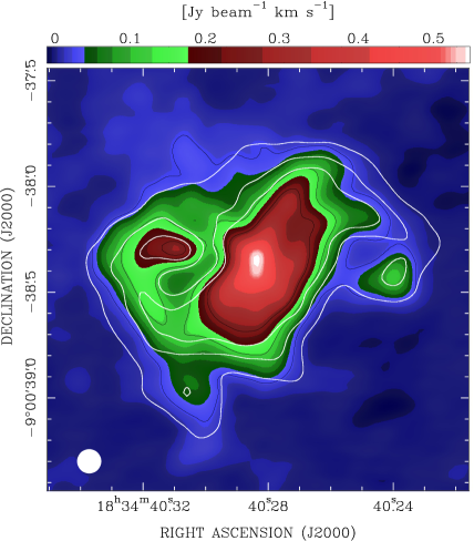
Figure 6: Moment-zero map of the CH₃CN ($19_{4}$–$18_{4}$) emission (colors and black contours) for a direct comparison with the CH₃OH ($14_{1,13}$–$14_{0,14}$) A⁺ emission of Fig. 1 (white contours). These CH₃CN and CH₃OH transitions have similar excitation energies (E_up) of 281.9 K and 260.2 K, respectively, and the line emission has been integrated over the same velocity range. The upper wedge quantifies the line intensity from its peak to the maximum negative in the map; black contours are drawn at levels of 10, 50, and 100 times the 1 $\sigma$ rms of 2.5 mJy beam^-1 km s^-1. We note that the white and black contours should be used for a direct comparison between the spatial morphology of the CH₃OH and CH₃CN emissions, respectively, because they correspond to relative levels of comparable rms (at variance with the color map which depends on the maximum in the map). The synthesized ALMA beam is shown in the bottom left corner.

In Fig. 1, we present the brightness map of a CH₃OH line at 349.107 GHz with an excitation energy of 260 K, which is the brightest line emission in our band. The emission was integrated in velocity around ($\pm$2 km s^-1) the line peak to emphasize the gas spatial distribution; this emission extends within a radius of approximately 3000 au from the young massive star in the region (star symbol) at the current sensitivity. For comparison with our cycle-3 ALMA observations, we draw the disk midplane at three radii as marked in Fig. 1 of Sanna et al. (2019), from the central star position to 1000 au (yellow), from 1000 to 2000 au (black), and up to 3000 au (magenta). In Fig. 2, we plot the same image rotated clockwise by $57\degr$, in order to align the (projected) outflow direction with the vertical axis of the plot. The CH₃OH emission is centrally peaked near (but offset from) the star, and outlines two apparent spiral features which extend on each side of the disk midplane. In Fig. 6, we also show that the CH₃CN gas has a similar spatial distribution at a similar excitation temperature (for K $=$ 4). In Fig. 7, we present a continuum map of the dust emission at the center frequency of 349.150 GHz, where the contours of Fig. 1 have been superposed for comparison.

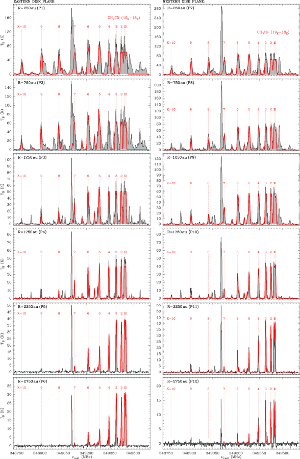
Figure 8: Spectra of the CH₃CN ($19_{K}$–$18_{K}$) transitions along the eastern (left column) and western (right column) sides of the disk plane. Spectra are integrated at radial steps of 500 au as indicated in Fig. 1, and each pointing is labeled on the top left accordingly. CH₃CN components, with K ranging from 0 to 10, are marked in red in each spectrum. The brightest line at a rest frequency of 349.107 GHz corresponds to the CH₃OH ($14_{1,13}$–$14_{1,14}$) A⁺ emission imaged in Fig. 2. Modeled spectra are overplotted in red; note that the first four K components were not fitted, except at positions P6 and P12 (cf. Sect. 3).

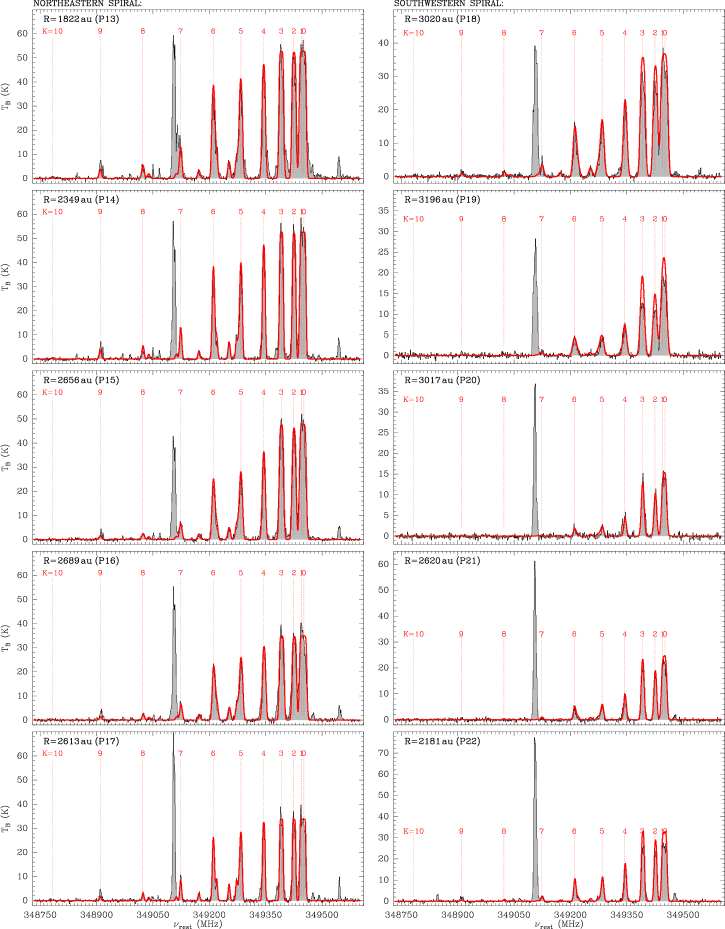
Figure 9: Same as Fig. 8, but for spectra of the CH₃CN ($19_{K}$–$18_{K}$) transitions along the northeastern (left column) and southwestern (right column) spirals.

We have extracted the integrated spectra at 22 distinct positions in the frequency range 348.7 to 349.5 GHz; this range includes the K-ladder of the 19 $\to$ 18 rotational transition of the CH₃CN molecule and its isotopologue CH${}_{3}^{13}$CN (Table 3). Each position covers a circular area of radius 250 au and they are plotted and labeled with white numbers in Fig. 1; these positions are used to sample the disk midplane and its apparent spiral features and, hereafter, are referred to as P1, P2,…, P22. Examples of the CH₃CN spectra are shown and analyzed in Fig. 2, while the complete set of 22 spectra is reported in Figs. 8 and 9. We analyzed these spectra in two steps.

In step-1, we made use of the Weeds package of GILDAS (Maret et al. 2011) to reproduce the CH₃CN and CH${}_{3}^{13}$CN spectra and estimate the physical conditions of the emitting gas. Under the assumption of local thermodynamic equilibrium (LTE), and accounting for the continuum level, Weeds produces a synthetic spectrum of an interstellar molecular species, depending on five parameters: (i) the intrinsic full width at half maximum (FWHM) of the spectral lines; (ii) the line offset with respect to the rest velocity in the region; (iii) the spatial extent (FWHM) of the emitting region, assumed to have a Gaussian brightness profile; (iv) the rotational temperature and (v) column density of the emitting gas. We fixed parameters (i) and (ii) by fitting a Gaussian profile to five K-components simultaneously, which are forced to have same linewidth and whose separation in frequency is set to the laboratory values (command MINIMIZE of CLASS). This procedure assumes that each spectral component is excited within the same parcel of gas. This “observed” linewidth was used to derive the “intrinsic” linewidth by correcting iteratively for the opacity broadening, with the opacity computed by Weeds (e.g., Eq. 4 of Hacar et al. 2016). Parameter (iii) was varied about the beam size at discrete steps of 5 mas; emission at the same distance from the star was forced to have same size (only within the midplane). This assumption was verified a posteriori based on the fit convergence (step-2). The same set of parameters was used to compute the spectra of CH₃CN and CH${}_{3}^{13}$CN species, whose relative abundance is set to 30 (Wilson & Rood 1994; Sanna et al. 2014).

In step-2, we input the initial parameters estimated with Weeds into MCWeeds (Giannetti et al. 2017), which implements a Bayesian statistical analysis for an automated fit of the spectral lines. We made use of a Monte Carlo Markov chains method to minimize the difference between the observed and computed spectra and derive the rotational temperature (iv) and column density (v) of the emitting gas with their statistical uncertainties. Parameters (i), (ii), and (iii) were fixed from step-1. The following additional criteria apply: we fitted simultaneously optically thin and partially opaque spectral lines with opacity lower than 5; the CH₃CN K $=$ 0–3 components were excluded from the fit (except for P6 and P12), because their profiles show signs of either filtering or an excess of warm envelope emission (e.g., side panels in Fig. 2; cf. Appendix B of Ahmadi et al. 2018); the number of lines processed by MCWeeds is $\geq 7$ for each pointing.

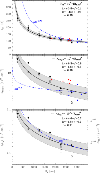
Figure 3: Dependence of the gas physical conditions with the projected distance from the star, as determined from the relative intensities of the CH₃CN and CH${}_{3}^{13}$CN lines near 349 GHz. Filled and empty black circles mark measurements in the eastern and western disk sides, and red and blue diamonds mark measurements in the northeastern ad southwestern apparent spirals, respectively (Table 2). Error bars of (only) midplane measurements are drawn, which account for an additional 10% uncertainty due to the assumptions. Upper panel: Temperature distribution along the disk midplane as a function of the projected distance from the star. The dotted bold line traces the $\chi^{2}$ fit to the sample distribution; the gray shadow shows the dispersion about the best fit ($1\sigma$). The best fit parameters and the linear correlation coefficient are indicated in the upper right. For comparison, the dashed blue line draws the increase of temperature with radius for a “classical” power-law dependence (R^-0.75). Middle panel: similar to the upper panel, but for the column density values. A logarithmic scale is used for the $y$-axis. Lower panel: similar to the upper panels, but for the H₂ volume density averaged along the line-of-sight; this is calculated by assuming an edge-on disk geometry. The right axis provides the conversion to g cm^-3.

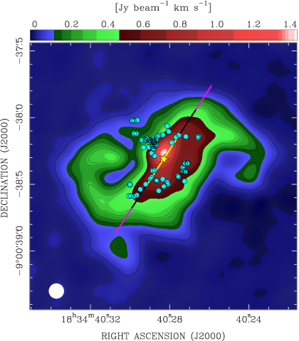
Figure 10: Same as Fig. 1, but, for comparison, the positions of the 6.7 GHz CH₃OH maser cloudlets are overplotted with cyan dots (from Sanna et al. 2010, 2015).

Notably, in more than half of the 22 spectra of Figs. 8 and 9, the methanol line at the center of the band stands brighter than the CH₃CN lines at low excitation energies. Their emission is optically thick and sets an upper limit to the expected maximum brightness from gas in LTE. Assuming that the CH₃OH and CH₃CN molecular species are fully coupled and emit cospatially, this is evidence that the CH₃OH ($14_{1,13}-14_{0,14}$) A⁺ transition is emitting by maser excitation, which adds to a plateau of thermal emission. In this context, we remind that G023.01$-$00.41 is among the brightest Galactic CH₃OH maser sources at 6.7 GHz, and, for comparison, in Fig. 10 we overplot to Fig. 1 the positions of the 6.7 GHz maser cloudlets derived at milliarcsecond accuracy by Sanna et al. (2010, 2015). The distributions of the emission in different CH₃OH maser lines usually resemble each other closely, and this evidence is confirmed in Fig. 10 where, for instance, the brightest emission in both transitions clusters on the western side of the disk. Also, we note that the same 349.1 GHz CH₃OH transition was found to emit by maser excitation around the early-type young star, S255 NIRS3 (Zinchenko et al. 2018).

In Table 2, we summarize the properties of the line and continuum emission associated with each of the 22 spectra: column 1 identifies each position as labeled in Fig. 1; columns 2 and 3 list the offset positions with respect to the phase center of the observations (Table 1); column 4 quantifies the (projected) linear distance of the center of each pointing from the star position, as defined in Sanna et al. (2019); column 5 lists the integrated continuum flux at 860 $\mu$m associated with each pointing, as measured from Fig. 7; columns 6 to 10 list the best fit parameters of the gas emission output by MCWeeds with their statistical uncertainties, with column 11 specifying the opacity of the CH₃CN K $=$ 4 line; columns 12 and 13 list the gas mass and H₂ column density estimated from the dust continuum emission within an area of 500 au diameter. This calculation assumes that the dust emission is optically thin at an equilibrium temperature equal to that listed in column 8, with a standard gas-to-dust mass ratio of 100, and a uniform dust absorption coefficient of 1.98 cm ² g^-1 at the observing frequency, obtained for thick ice mantles, densities of 10⁸ cm^-3, and linearly interpolated from the values tabulated by Ossenkopf & Henning (1994). The validity of this assumption will be commented in Sect. 4.1.

Although the synthetic spectra reproduce the bulk of the emission very well (red profiles in Figs. 8, 9), discrepancies between the observed and expected emission of the higher K lines exist at the inner disk radii, where molecular chemistry is rich and contamination from different molecular species is expected (e.g., CH₃OCHO, cf. Liu et al. 2020). Also, towards these regions the line of sight crosses large portions of gas at different distances from the star, and one can expect that the integrated emission will be the combination of different gas physical conditions. Then, the working hypothesis we have done, that only a single temperature and density component exists, may not be fully satisfied, and local gradients of both temperature and density might affect the observed line profiles. This second order effect is neglected in the following analysis and will contribute to the uncertainty in the assumptions.

4 Discussion

4.1 Physical conditions

Having on hand the information about the gas physical conditions across the extent of the disk, in the following we want to study the dependence of the gas temperature, column and volume densities with distance from the central star. In Fig. 3, we present a diagram for each of these three quantities plotted against the projected distance (listed in column 4 of Table 2), where disk loci are marked with different symbols: filled and empty black circles are used for the eastern and western disk sides, respectively, and red and blue diamonds for the northeastern and southwestern apparent spirals, respectively. We explicitly note that the uncertainties reported in Table 2 quantify statistical errors only, meaning that they hold under the assumptions used for the analysis. While the statistical errors convey information on the quality of the assumptions, they do not consider the uncertainties inherent in the assumptions themselves, which can be of the order of 10% on average. Error bars plotted in Fig. 3 account for a nominal uncertainty of 10% summed in quadrature to the statistical errors.

In the upper panel of Fig. 3, we show that the local gas temperature and the distance from the star are related to each other by a power-law of exponent $-0.43$ $\pm$0.03, and this relation is isotropic and verified both within the disk midplane and the apparent spirals. The dotted bold line draws the best fit to the data points, obtained by minimizing a linear relation between the logarithms of the gas temperature and radius, $\log_{10}(\rm T_{ex})=k\,{\cdot}\,\log_{10}(\rm R_{p})+h$. The gray shadow marks the dispersion about the best fit ($1\sigma$). Values of $k$ and $h$ are reported in the plot with their uncertainties, together with the linear correlation coefficient of the sample distribution ($r$ $=$ 0.98). Only for the sake of comparison, we draw a “classical” temperature dependence with radius as R^-3/4, which is expected for geometrically thin disks heated externally by the star or internally by viscosity (e.g., Kenyon & Hartmann 1987); this curve starts with the same temperature (98.4 K) of the best fit at 3000 au (the estimated outer disk radius).

In the middle panel of Fig. 3, we plot the CH₃CN column density, in units of 10¹⁶ cm^-2, with respect to the same distance scale. The dotted bold line draws the best fit to the sample distribution, similar to the upper panel, and the best fit parameters are reported in the plot with their uncertainties. In comparison with the upper panel, the data points are still strongly correlated (0.90), but show a steeper slope with a relative dispersion three times larger. Column densities along the apparent spiral arms are also consistent with the power law measured along the midplane. At variance, the dashed blue line shows a shallower increase scaling with R^-0.5, as it would be expected for a spherical distribution of gas (e.g., an envelope/core) with density profile proportional to R^-1.5; this curve starts with the same column density (9.2 $\times$ 10¹⁵ cm^-2) of the best fit at 3000 au.

In the lower panel of Fig. 3, we can evaluate the average volume density of H₂ gas along the line-of-sight, ¡$\rho_{H_{2}}$¿, under the assumption that the central star is surrounded by a circular gaseous disk observed approximately edge-on, that has a sharp cutoff at radii of 3000 au (R_max). At each of the 12 pointings in the midplane, we divide the CH₃CN column density value by the local disk length intercepted by the observer, $2\times(R_{\rm max}^{2}-R_{\rm p}^{2})^{0.5}$, where $R_{\rm p}$ is the projected distance of each pointing from the star position (as listed in Table 2). In the calculation, we assume a constant relative abundance of 10^-8 between CH₃CN and H₂ species for temperatures above 100 K, for consistency with previous work (e.g., Johnston et al. 2020; Ahmadi et al. 2019). The best fit parameters are reported in the plot with their uncertainties, with the volume density in units of 10⁸ cm^-3. The volume density fit implies an average of 1.8 $\times$ $10^{7}$ cm^-3 at a radius of 3000 au, which increases to 8.2 $\times$ $10^{8}$ cm^-3 at ten times smaller (projected) distance from the star.

The average volume density evaluated at the projected radius ($R_{\rm p}$) of 250 au is a robust underestimate for the gas density in the inner disk regions. At the corresponding positions (P1 and P7 in Fig. 1), the line-of-sight crosses a large range of disk radii, from the outer disk regions down to 250 au. We can still exploit this average volume density to obtain a better approximation for the peak density at 250 au from the star. The average integral of the best fit power-law, $\frac{1}{(a-b)}\int_{b}^{a}10^{4.6}\,\times\,R^{-1.5}dR$, would equal a volume density of 8.2 $\times$ $10^{8}$ cm^-3 by definition, when evaluated from 3000 ($a$) to 250 au ($b$). By solving this equation at the inner radius, one derives a peak density of 4.8 $\times$ $10^{9}$ cm^-3 (or 1.6 $\times$ $10^{-14}$ g cm^-3) which is approximately a factor of 6 higher than the average.

In column 12 and 13 of Table 2, we have estimated the mass and column density of H₂ gas from the dust continuum fluxes at 860 $\mu$m, assuming the dust emission is optically thin. However, the dust emission is optically thick at these wavelengths (with dust opacity of the order of unity and higher), as it can be inferred by comparing the low brightness temperature of the continuum (of only a few 10 K at the peak) with respect to the molecular line estimate ($\approx$ 300 K). As a consequence, the dust continuum fluxes are only representative of emission in the envelope outskirts and do not probe the inner disk regions, at variance with the CH₃CN line emission at high excitation energy.

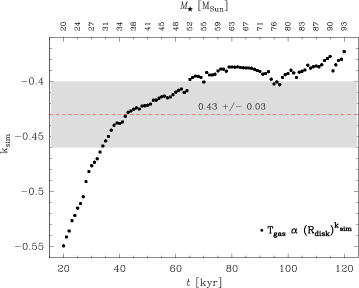
Figure 4: Variation of the temperature slope with time, as determined at the disk midplane of a massive star with the simulations by Kuiper & Hosokawa (2018, their Fig. 6), with the corresponding stellar mass indicated on top. k_sim is the mean linear variation determined over the range of radii, 100–2000 au. The red dashed line marks the observed value fitted in the upper panel of Fig. 3, and the gray shadow defines the dispersion about the best fit ($1\sigma$).

4.1.1 Model comparison

We can compare the above quantities with those derived in recent hydrodynamics simulations by Kuiper & Hosokawa (2018), who simulated the growth of a massive star under the influence of its own radiation field and the effect of photoionization on the circumstellar medium. Their Fig. 6 describes the evolution in time of the gas physical conditions along the disk midplane, as a function of the radius from the star.

The average volume density in the lower panel of Fig. 3 herein is diluted along the line-of-sight and it is systematically lower than the volume density expected at an actual radius equal to the projected radius (R_p). Therefore, we corrected the volume density at a projected radius of 250 au and calculated a peak density of 1.6 $\times$ $10^{-14}$ g cm^-3 (see Sect. 4.1): this estimate is in excellent agreement with the density predicted by the simulations at the same radius, within a factor of 2.

In Fig. 4, we present a plot of the temperature slope at the disk midplane (k_sim $=$ $\frac{\partial\log_{10}(\rm T)}{\partial\log_{10}(\rm R)}$) as a function of time, as derived from the simulations by Kuiper & Hosokawa (2018, their Fig. 6). The slope is defined by linear fitting the change of temperature with radius in the distance range 100–2000 au, and varies (almost) monotonically over a small range between $-0.55$ and $-0.37$. The axis on top indicates the corresponding stellar mass at a given time. The steeper slope at early times describes the settling of a very-young (with lower mass) accreting star and the formation of its circumstellar disk. The observed slope is fully consistent with the model expectation and is drawn with a dashed line in Fig. 4 for comparison. The magnitude of the modeled temperature at a given radius depends on the stellar mass. In Fig. 6 of Kuiper & Hosokawa (2018), the temperature at a radius of 250 au increases with time from 300 K to 500 K, when the stellar mass approximately increases from 20 M_⊙ to 100 M_⊙. The lower end of this range is consistent with the combination of stellar mass (20 M_⊙) and disk temperature (289 K) of our observations within the uncertainties, suggesting that the stellar system is still in a very early stage of evolution ($<$ 40 kyr).

The comparison above shows that those basic quantities, obtained for the model and with our observations independently, are consistent with each other and validates these conditions for future model developments.

4.2 Disk stability

In the following, we want to study whether opposite forces are in equilibrium inside the accretion disk, or whether self-gravity might dominate locally causing the disk to fragment. For this purpose, we apply the analysis by Kratter et al. (2010) who describe the stability of a disk where gas is falling in rapidly, as it is observed in the target source. In Sanna et al. (2019), we quantified a mass infall rate of $6\times 10^{-4}$ M_⊙ yr^-1 by comparing position-velocity diagrams observed along the disk midplane with synthetic diagrams simulated through a dedicated disk model.

Following Kratter et al. (2010), we have calculated two dimensionless accretion rates describing the state of the system. The first “rotational” parameter, $\Gamma$ $=$ $\rm\dot{M}_{inf}\cdot(M_{sys}\cdot\Omega)^{-1}$, relates the accretion timescale to the orbital timescale of infalling gas, where $\rm\dot{M}_{inf}$, $\rm M_{sys}$, and $\Omega$ are the mass accretion rate, the system mass of star plus disk at a given radius, and the angular velocity at the same radius, respectively. The second “thermal” parameter, $\xi$ $=$ $\rm\dot{M}_{inf}\cdot G\cdot c_{s}^{-3}$, relates the mass accretion rate to the local sound speed of disk material. $\rm\dot{M}_{inf}$ and M${}_{sys}(R)$ were quantified in Sanna et al. (2019); $\Omega(R)$ is evaluated based on the enclosed mass at a given radius and considering an orbital motion which is either Keplerian or 70% of its value; $c_{s}$ is evaluated from the excitation temperatures in Table 2. These parameters are calculated for each of the 22 pointings marked in Fig. 1, and are plotted in Fig. 5 for a direct comparison with Fig. 2 of Kratter et al. (2010).

In Fig. 5, the upper and lower panels describe the state of the system for a sub-Keplerian and Keplerian rotation curve, respectively. We have demonstrated that the system is sub-Keplerian outside of 500 au from the central star and might approach centrifugal equilibrium inside this radius (Sanna et al. 2019). For this reason, we expect the system to behave in between these two extremes. The diagram is divided in two regions where the system is either stable (white) or prone to fragmentation (grey); this empirical boundary condition is defined at $\Gamma$ $=$ $\rm\xi^{2.5}\cdot 850^{-1}$ (Kratter et al. 2010). $\Gamma-\xi$ couples characterizing the disk midplane are labeled according to the numbers in Fig. 1; $\Gamma-\xi$ couples characterizing the apparent spiral features are grouped over a small range of values in the plot and are indicated with red and blue diamonds for clarity (same symbols as in Fig. 3).

This analysis outlines that $\Gamma-\xi$ couples are distributed near the boundary between a stable and unstable disk, and the accretion disk meets the condition for fragmentation marginally along its whole extent. Regions beyond 1000 au are progressively more unstable and have the higher likelihood to produce stellar companions. The parameter $\xi$ depends on T^-3/2 through the sound speed, and explains the small shifts between the warmer western side of the disk and the colder eastern side (by approximately 10 K). The disk temperature increases with time by tens to hundreds of Kelvin due to the growing stellar mass, and, as a consequence, thermal pressure would act to stabilize the disk whose position would shift to the left side of the diagram. Concurrently, the disk gains mass and increases its Keplerian radius as time passes (Kuiper & Hosokawa 2018, their Fig. 7), so that the outer disk regions will accelerate from sub-Keplerian (Fig. 5, upper panel) to Keplerian rotation (Fig. 5, lower panel) on average. The parameter $\Gamma$ decreases by increasing the mass accreted by the star plus disk and its angular velocity: such a variation makes the disk shifts in the diagram to a less stable configuration (cf. Sect. 4 of Kratter et al. 2010 for the relation to the Toomre parameter). Whether or not the system will grow more unstable in time as an overall effect, it is difficult to predict without further information about, for instance, the history of the system, which might have already developed internal fragments in the past.

From a theoretical point of view, and in agreement with our snapshot taken in Fig. 5, unstable accretion disks are a robust product of distinct models simulating the formation of massive stars (e.g., Kratter et al. 2010; Klassen et al. 2016; Rosen et al. 2016; Harries et al. 2017; Meyer et al. 2017, 2018; Rosen et al. 2019; Ahmadi et al. 2019; Oliva & Kuiper 2020). Unstable disks can fragment leading to hierarchical star systems that consist of (several) low-mass stellar companions surrounding a massive primary. These simulations also predict that unstable accretion disks will develop substructures and density-enhanced spiral features, which wrap along the equatorial plane. In the following section, we comment on the apparent spiral morphology imaged in Fig. 1.

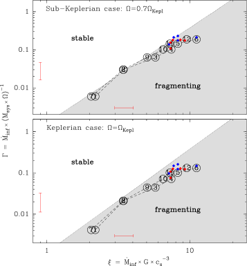
Figure 5: Analysis of the disk stability against local fragmentation, following the methodology outlined in Kratter et al. (2010). The plot reports the dependence of two dimensionless parameters, $\Gamma$ and $\xi$, whose relation defines two regions where the disk is stable (white) or prone to fragmentation (grey). Black empty circles mark the local values of $\Gamma$ and $\xi$ within the midlplane and are labeled according to the pointing numbers in Table 2 (P2 and P8 overlap); red and blue diamonds mark values for the northeastern and southwestern apparent spirals, respectively. The upper and lower plots compare the behavior for an angular velocity ($\Omega$) which is either 70% of (upper), or equal to (lower), the Keplerian value. Reference error bars are indicated in red for an inner position (largest ticks in logarithmic scale), and account for a 10% uncertainty in the local temperature and a positional uncertanty of half the beam size.

4.2.1 Spiral arms or accretion streams?

Spiral arms can be produced by gravitational instabilities, being the manifestation of underlying density waves in a self-gravitating disk (e.g., Lodato & Rice 2005), and by tidal interactions between the disk and a cluster companion, either internal or external to the disk itself (e.g., Zhu et al. 2015).

From an observational point of view, evidence for disk substructures have been recently reported towards a couple of massive young stars (Maud et al. 2019; Johnston et al. 2020). In particular, Johnston et al. (2020) have outlined the existence of a spiral arm branching off the disk of a massive star at varying pitch angle (20$\degr$–47$\degr$). Arguably, the asymmetric spiral morphology they found could be triggered by tidal interactions with cluster companions (e.g., Forgan et al. 2018).

In order to interpret the apparent spiral morphology imaged towards G023.01$-$00.41, we have to take into account the viewing angle to the observer. In Fig. 2, the horizontal axis of the plot approximately coincides with the equatorial plane of the disk, whose inclination was inferred to be nearly edge-on. Consequently, the vertical axis of the plot provides approximate altitudes above the disk midplane, implying that the apparent spiral features extend up to 2500-3000 au off the plane (up to 3500 au in the limit of 30$\degr$ inclination). This evidence suggests that the apparent spiral features might be rather streams of gas producing a warp in the outer disk regions and, hereafter, we refer to the northeastern and southwestern apparent spirals as the northeastern and southwestern streams, respectively. Whether these streams of gas are due to inward or outward motions can be tested based on the line fitting presented in Sect. 3.

The combined fitting over a group of spectral lines, emitting from the same spatial region, allows us to determine the offset velocity (v_off) of local gas with an accuracy better than $0.1$ km s^-1 (column 6 of Table 2). This analysis reveals two velocity gradients of the order of 1 km s^-1 per 2000 au along the northeastern (positions 13 to 16) and southwestern (positions 19 to 22) streams. Gas accelerates from the ambient velocity in the outer stream regions, at about 79 km s^-1, to blueshifted velocities close to the disk plane. If disk material were moving outward, as due to a disk wind, one would expect the gas velocity to be very different from the ambient velocity at the stream tip. On the contrary, these velocity gradients are consistent with a scenario where gas accelerates towards the disk moving from the outer envelope at the ambient velocity, and supporting the existence of an accretion flow. This scenario naturally explains the infall profile previously detected in the position-velocity diagrams along the disk midplane (Sanna et al. 2019, their Fig. 5). At positions P17 and P18, the measured velocity differs from that expected for a regular gradient along the entire streams. This discrepancy can be interpreted as an effect of contamination from the outer disk gas at position P17, and the local gas dynamics at position P18 (see further discussion below). For completeness, we also mention a third scenario where the apparent spiral features might just be overdensities within the larger envelope around the disk, although we consider this hypothesis very unlikely given the spatial morphology and physical conditions observed.

Explaining the three-dimensional morphology of the accretion streams prompts for a dedicated theoretical ground which goes beyond the scope of the current paper. Therefore, in the following we highlight a number of observational features which should be taken into account in future dedicated simulations. First, the northeastern and southwestern streams appear approximately symmetric in gas emission but not in dust, with the southwestern stream being deficient in continuum emission with respect to the northeastern stream (Fig. 7). Whether this difference is related to the origin of the streams themselves should be clarified. Second, to the east of the accretion disk, at a (projected) distance of approximately 3500 au from the star, the continuum map shows a dust overdensity which also coincides with a local peak of molecular emission, labeled as “mm2” in Fig. 2. Whether and how this source could perturb the stream morphology and affect the local warp of the disk should be clarified. Finally, we note that the outer tips of both streams are the regions with the higher combination of column density and temperature along the streams (P13 and P18 of Table 2). Simulations of in-plane spiral arms show that their overdensities can fragment leading to companion stars that, in turn, can influence the morphology of disks and spirals (e.g., Fig. 1 and 12 of Oliva & Kuiper 2020). By analogy, we pose the question of whether or not the stream tips could host newly formed stars, and, if yes, how they could interact with the stream morphology.

5 Conclusions

We report on spectroscopic Atacama Large Millimeter/submillimeter Array (ALMA) observations near 349 GHz with a spectral and angular resolutions of 0.8 km s^-1 and $0\aas@@fstack{\prime\prime}1$, respectively. We targeted the star-forming region G023.01$-$00.41 and imaged the accretion disk around a luminous young star of $10^{4.6}$ L_⊙ in both methyl cyanide and methanol emission. We have fitted the K-ladder of the CH₃CN ($19_{K}$–$18_{K}$) transitions, and that of the isotopologue CH${}_{3}^{13}$CN, to derive the physical conditions of dense and hot gas within 3000 au from the young massive star. Our results can be summarized as follows:

1. We have resolved the spatial morphology of the accretion disk which shows two apparent spiral arms in the disk outskirts at opposite sides (Fig. 2, main). These apparent spirals likely represent streams of accretion from the outer envelope onto the disk. They appear almost symmetric in molecular gas but not in dust, with one stream being deficient in continuum emission with respect to the other (Fig. 7). The disk is remarkably bright in CH₃OH ($14_{1,13}-14_{0,14}$) A⁺ emission showing a maser contribution up to (at least) 2000 au from the young star.

2. We have derived the temperature, column and volume densities of molecular gas along the disk midplane and accretion streams, and studied their dependence with distance from the central star (Fig. 3). The gas temperature varies as a power law of exponent R^-0.43, which is significantly shallower than that expected around Solar-mass stars (R^-0.75). The volume density averaged along the line-of-sight through the disk varies as a power law of exponent R^-1.5; this slope implies a peak density of 1.6 $\times$ $10^{-14}$ g cm^-3 at 250 au from the star.

3. Our findings are in excellent agreement with the results of recent hydrodynamics simulations of massive star formation (Kuiper & Hosokawa 2018), and this comparison supports the idea we are tracing disk conditions as opposed to envelope conditions. In turn, this comparison provides evidence that the high excitation-energy transitions of CH₃CN allow us to peer into the inner disk regions.

4. We have studied whether the disk is stable against local gravitational collapse following the analysis by Kratter et al. (2010), who describe the stability of a disk undergoing rapid accretion. This analysis outlines that the accretion disk marginally meets the condition for fragmentation along its whole extent, and regions beyond radii of 1000 au are progressively more unstable and have the higher likelihood to produce stellar companions (Fig. 5). Notably, the tips of the accretion streams are the loci of higher temperature and column density, and could be hosting young stars in the making. The fact that the disk is gravitationally unstable, together with the effect of tidal interactions with cluster member(s), might be the origin of disk substructures to be probed by observations of optically-thin dust emission.

These observations provide direct constraints for models trying to reproduce the formation of stars of tens of Solar masses, with particular focus on the disk properties, the spatial morphology of gas accreting onto the disk, and the perspective of forming a tight cluster of stellar companions.

Appendix A Additional material

Table 3: Observed lines

$\nu$	Species / Line	Eup
(GHz)		(K)
CH3CN
348.784	CH3CN ($19_{10}-18_{10}$)	880.6
348.911	CH3CN ($19_{9}-18_{9}$)	745.4
349.024	CH3CN ($19_{8}-18_{8}$)	624.3
349.125	CH3CN ($19_{7}-18_{7}$)	517.4
349.212	CH3CN ($19_{6}-18_{6}$)	424.7
349.286	CH3CN ($19_{5}-18_{5}$)	346.2
349.346	CH3CN ($19_{4}-18_{4}$)	281.9
349.393	CH3CN ($19_{3}-18_{3}$)	232.0
349.426	CH3CN ($19_{2}-18_{2}$)	196.3
349.446	CH3CN ($19_{1}-18_{1}$)	174.8
349.453	CH3CN ($19_{0}-18_{0}$)	167.7
CH${}_{3}^{13}$CN
348.853	CH${}_{3}^{13}$CN ($19_{8}-18_{8}$)	624.3
348.953	CH${}_{3}^{13}$CN ($19_{7}-18_{7}$)	517.3
349.040	CH${}_{3}^{13}$CN ($19_{6}-18_{6}$)	424.6
349.113	CH${}_{3}^{13}$CN ($19_{5}-18_{5}$)	346.1
349.173	CH${}_{3}^{13}$CN ($19_{4}-18_{4}$)	281.9
349.220	CH${}_{3}^{13}$CN ($19_{3}-18_{3}$)	231.9
349.254	CH${}_{3}^{13}$CN ($19_{2}-18_{2}$)	196.2
349.274	CH${}_{3}^{13}$CN ($19_{1}-18_{1}$)	174.8
349.280	CH${}_{3}^{13}$CN ($19_{0}-18_{0}$)	167.7
CH3OH
349.107	CH3OH ($14_{1,13}-14_{0,14}$) A+	260.2

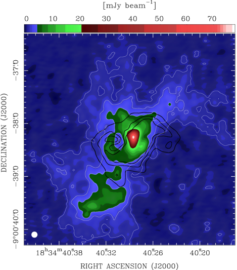
Figure 7: Dust continuum emission at 860 $\mu$m (colors and white contours) imaged with ALMA towards G023.01$-$00.41 and derived from 52 MHz of emission-free band in the spectra. The upper wedge quantifies the continuum brightness from its peak to the maximum negative in the map; white contours are drawn at levels of 3, 10, and 20 times the 1 $\sigma$ rms of 0.2 mJy beam^-1. The moment-zero map of the CH₃OH ($14_{1,13}$–$14_{0,14}$) A⁺ mission is overlaid with the same black contours of Figs. 1 and 2 for comparison. The synthesized ALMA beam is shown in the bottom left corner.