Quantum Generalized Hydrodynamics of the Tonks-Girardeau gas:
density fluctuations and entanglement entropy

Abstract

We apply the theory of Quantum Generalized Hydrodynamics (QGHD) introduced in [Phys. Rev. Lett. 124, 140603 (2020)] to derive asymptotically exact results for the density fluctuations and the entanglement entropy of a one-dimensional trapped Bose gas in the Tonks-Girardeau (TG) or hard-core limit, after a trap quench from a double well to a single well. On the analytical side, the quadratic nature of the theory of QGHD is complemented with the emerging conformal invariance at the TG point to fix the universal part of those quantities. Moreover, the well-known mapping of hard-core bosons to free fermions, allows to use a generalized form of the Fisher-Hartwig conjecture to fix the non-trivial spacetime dependence of the ultraviolet cutoff in the entanglement entropy. The free nature of the TG gas also allows for more accurate results on the numerical side, where a higher number of particles as compared to the interacting case can be simulated. The agreement between analytical and numerical predictions is extremely good. For the density fluctuations, however, one has to average out large Friedel oscillations present in the numerics to recover such agreement.

I Introduction

I.1 Hydrodynamics, quantum fluctuations, and equal-time correlations

Hydrodynamics offers a powerful way of thinking about the dynamics of many-body systems on macroscopic scales Landau and Lifshitz (1987); Spohn (2012). While made of microscopic constituents that typically undergo complex collective dynamics, fluids of many particles are viewed as continuous media on larger scales. Their evolution is encoded in the time- and spatial-dependence of a small number of local thermodynamic quantities, or hydrodynamic variables, such as particle density, energy density, or more generally densities of conserved charges in the system. In that effective description at the macroscopic scale, the microscopic degrees of freedom are not immediately visible, but instead they are reflected in long wavelength variations of the charge densities. In particular, around an equilibrium configuration, small variations of the charge densities propagate through the fluid as sound waves. These sound waves are the relevant collective degrees of freedom at low energy.

The basic ideas of hydrodynamics apply to fluids made of classical or quantum constituents alike. For instance, the Euler equations for a Galilean-invariant one-dimensional (1D) fluid with conserved particle number and momentum typically read, in conservative form,

$$\left\{\begin{array}[]{rcl}\partial_{t}\rho+\partial_{x}(\rho u)&=&0\\ \partial_{t}(m\rho u)+\partial_{x}(m\rho u^{2}+\mathcal{P}(\rho))&=&-\rho\partial_{x}V.\end{array}\right.$$ (1)

Here $\rho(x,t)$ is the particle density, $u(x,t)$ is the mean fluid velocity, $m$ is the particles mass, $V(x)$ is an external potential that acts as a source term for the momentum density $m\rho u$ according to Newton’s second law, and $\mathcal{P}(\rho)$ is the equilibrium pressure computed in the underlying microscopic model. This microscopic model can be either classical or quantum: the Euler equations (1) are applicable to a classical gas at constant temperature, for instance in contact with a thermostat; they are also applicable to quantum gases at zero temperature Abanov (2006), in particular to the one-dimensional Bose gas with contact repulsion Doyon et al. (2017); Ruggiero et al. (2019). Apart from the specific function $\mathcal{P}(\rho)$ entering the momentum current in (1), which differs from one microscopic system to another, the form of the equations (1) is the same.

Differences between quantum and classical fluids arise at the level of their fluctuations. In a classical fluid at finite temperature, one expects the low-energy collective modes to have thermal fluctuations, and it is the goal of ‘fluctuating hydrodynamics’ approaches to capture these, see e.g. Landau et al. (1992); Swift and Hohenberg (1977); Forster (2018); Spohn (2014). In a quantum fluid at zero temperature, there are no thermal fluctuations, but the low-energy collective modes typically have quantum fluctuations. This is well illustrated starting from the Euler equations (1). For simplicity, consider the ground state of the spatially homogeneous system ($V(x)=0$), with $\rho(x,t)=\rho_{0}$ and $u(x,t)=0$. Linearizing the system (1) for small deviations $(\delta\rho(x,t),\delta u(x,t))$, one finds $\partial_{t}\delta\rho+\rho\partial_{x}\delta u=0$ and $\partial_{t}\delta u+\frac{1}{m\rho}\frac{\partial\mathcal{P}}{\partial n}\partial_{x}\delta\rho=0$, or equivalently

$$\left(\frac{\partial}{\partial t}-\left(\begin{array}[]{cc}+v&0\\ 0&-v\end{array}\right)\frac{\partial}{\partial x}\right)\left(\begin{array}[]{c}\pi\,\delta\rho+K\frac{m}{\hbar}\,\delta u\\ \pi\,\delta\rho-K\frac{m}{\hbar}\,\delta u\end{array}\right)\,=\,0,\qquad\quad{\rm with}\quad v:=\sqrt{\frac{1}{m}\frac{\partial\mathcal{P}}{\partial\rho}},\qquad K:=\frac{\pi\hbar\rho}{mv}.$$ (6)

Here $v$ is the sound velocity in the fluid, and $K$ is a dimensionless parameter. [$K$ is called the Luttinger parameter, and it is normalized such that $K=1$ in the Tonks-Girardeau (hard core) limit of the 1D Bose gas with contact repulsion]. We see from Eq. (6) that there are right- and left-moving sound waves, corresponding to specific linear combinations of $\delta\rho$ and $\delta u$ parameterized by $K$, traveling at velocity $\pm v$. The sound waves are then used as the basic ingredient in a quantized theory of the fluid described by the Euler equations (1). The basic idea is to look at $\delta\rho(x)$ and $\delta u(x)$ as operators $\delta\hat{\rho}(x)$, $\delta\hat{u}(x)$ in a quantum theory, and to impose the canonical commutation relations (Landau, 1941),

$$\left[\delta\hat{u}(x),\delta\hat{\rho}(y)\right]\,=\,\frac{\hbar}{im}\delta^{\prime}(x-y),$$ (7)

and $\left[\delta\hat{\rho}(x),\delta\hat{\rho}(y)\right]=\left[\delta\hat{u}(x),\delta\hat{u}(y)\right]=0$. To construct a Hamiltonian for these quantum fluctuations, one imposes that the Heisenberg equations $\partial_{t}\delta\hat{\rho}=\frac{i}{\hbar}[\hat{H},\delta\hat{\rho}]$ and $\partial_{t}\delta\hat{u}=\frac{i}{\hbar}[\hat{H},\delta\hat{u}]$ coincide with the equations of motion (6). This leads to

$$\hat{H}\,=\,\frac{\hbar v}{2}\int\left[\frac{K}{\pi}\left(\frac{m}{\hbar}\delta\hat{u}(x)\right)^{2}+\frac{\pi}{K}(\delta\hat{\rho}(x))^{2}\right]dx,$$ (8)

which is the Hamiltonian of a Luttinger liquid Giamarchi (2003); Cazalilla (2004); Tsvelik (2007). In conclusion, when one looks at quantum fluctuations of the collective modes (sound waves) of a standard Euler fluid in 1D, one arrives at the Luttinger liquid, which is the universal theory of 1D quantum hydrodynamics.

Physically, one consequence of the quantum fluctuations of the collective modes is that they induce equal-time correlations at different points in the fluid. For instance, the connected part of the density-density correlation in the ground state of the Hamiltonian (8) is  (Giamarchi, 2003; Cazalilla, 2004; Tsvelik, 2007):

$$\left<\delta\hat{\rho}(x_{1})\delta\hat{\rho}(x_{2})\right>_{\rm conn.}\,=\,\frac{-K}{2\pi^{2}(x_{1}-x_{2})^{2}}.$$ (9)

This is the leading power-law decay for the zero-temperature correlation of microscopic density observables in the model whose hydrodynamic equations are (1). Similarly, correlations of many other observables can be obtained from simple calculations within Luttinger liquid theory. We stress that the presence of such power-law correlation functions between observables at different macroscopic positions in the fluid is really a quantum effect. They are not accounted for in the classical fluid theory (1), which, by linear response, only predicts nonzero correlations in space-time at the velocities of sound mode propagation, under the Euler scaling $\lim_{\lambda\to\infty}\lambda\langle\delta\hat{\rho}(\lambda x_{1},\lambda t_{1})\delta\hat{\rho}(\lambda x_{2},\lambda t_{2})\rangle_{\rm conn.}$ De Nardis et al. (2021) in which (9) vanishes; and they are stronger than correlations that would occur at finite temperatures due to thermal fluctuations, which decay exponentially in space. This is even more obvious when one considers the entanglement between different pieces of the fluid. Classically there can be no entanglement. Yet, after quantum fluctuations have been incorporated in the theory, it makes sense to look at the entanglement entropy in the ground state of the Hamiltonian (8), leading to the well-known result for a subsystem of length $\ell$ Calabrese and Cardy (2004, 2009),

$$S(\ell)\,=\,\frac{1}{3} \log(\ell/\epsilon),$$ (10)

for some cutoff $\epsilon$. This shows that, despite the simplicity of the approach, quantizing the collective modes of the hydrodynamic equations (1) has the potential to reveal many features of the fluid that are truly quantum.

The classical Euler equations (1) describe a fluid with conserved particle number and momentum. When there are more conserved quantities, these two equations are complemented with more conservation equations, one for each additional conservation law. Remarkably, even when there are infinitely many conserved quantities, it is still possible to derive an Euler-scale description. This is ‘Generalized Hydrodynamics’ (GHD), the hydrodynamic theory of 1D integrable systems introduced in 2016 in two very influential papers by Castro-Alvaredo et al. Castro-Alvaredo et al. (2016) and by Bertini et al. Bertini et al. (2016).

In a recent paper, we asked the following question Ruggiero et al. (2020): What is the theory of quantum fluctuations around GHD? In other words: What happens if one mimics the derivation of quantum hydrodynamics above, replacing the standard Euler equations (1) that lead to a standard Luttinger liquid (8), by the GHD equations of Refs. Castro-Alvaredo et al. (2016); Bertini et al. (2016)?

The answer given in Ref. Ruggiero et al. (2020) is that the theory of quantum fluctuations around GHD is a multi-component, time-dependent and spatially inhomogeneous Luttinger liquid, where excitations propagate as the linear sound waves of the standard GHD theory. This setup was dubbed ‘quantum GHD’ in Ref. Ruggiero et al. (2020). [We note that some authors have expressed their preference for other names for that setup, e.g. for ‘generalized quantum hydrodynamics’ Alba et al. (2021). This terminology also makes sense, but to make the connection with our previous work Ruggiero et al. (2020) perfectly clear, we keep the name ‘quantum GHD’ in this paper.] Numerical comparisons of that theory with t-DMRG simulations for the 1D Bose gas at finite repulsion strength were presented in Ref. Ruggiero et al. (2020). In this follow-up paper, our goal is to investigate the special case of infinite repulsion (Tonks-Girardeau limit), which maps to non-interacting fermions Girardeau (1960), so it allows to do more analytical calculations and to perform more stringent tests of the theory. We focus in particular on spatial- and time-dependence of density correlations, and on the evolution of the entanglement entropy in the system. We obtain a number of analytical results that are exact in the hydrodynamic limit, and for which we provide extensive numerical checks (Fig. 2). We stress that as the Tonks-Girardeau limit is described by a free fermionic theory, whose hydrodynamic equations are linear, certain subtle correlation effects due to nonlinearities, discussed in Ruggiero et al. (2020), are not present. Although our techniques are, to some extent, similar to semiclassics and to other recent related works Dean et al. (2018, 2019); Smith et al. (2020, 2021), to our knowledge there exists no alternative method to arrive at our results.

I.2 This paper: tests of ‘quantum GHD’ in the Tonks-Girardeau gas

This paper is a follow-up of Ref. Ruggiero et al. (2020); we aim at clarifying some aspects of the results of Ruggiero et al. (2020) by analyzing the simple case of the Tonks-Girardeau gas in more details. We start from the 1d Bose gas with delta repulsion in an external potential $V(x,t)$, with the Hamiltonian Lieb and Liniger (1963); Berezin et al. (1964); Korepin et al. (1997)

$$\hat{H}(t)\,=\,\int dx\left(\frac{\hbar^{2}}{2}(\partial_{x}\hat{\Psi}^{\dagger})(\partial_{x}\hat{\Psi})+(V(x,t)-\mu)\hat{\Psi}^{\dagger}\hat{\Psi}+\frac{g}{2}\hat{\Psi}^{\dagger 2}\hat{\Psi}^{2}\right),$$ (11)

where $\hat{\Psi}^{\dagger}(x)$, $\hat{\Psi}(x)$ are operators that create/annihilate a boson at position $x$, and satisfy the canonical commutation rule $[\hat{\Psi}(x),\hat{\Psi}^{\dagger}(x^{\prime})]=\delta(x-x^{\prime})$. $\mu$ is the chemical potential, and we set the mass of the bosons to $m=1$. The hard core (or Tonks-Girardeau Girardeau (1960)) limit is given by

$$g\,\rightarrow\,+\infty.$$ (12)

In that limit, the Hamiltonian (11) maps to the one of non-interacting fermions through the non-local (Jordan-Wigner) transformation,

$$\hat{\Psi}_{F}^{\dagger}(x)\,=\,e^{i\pi\int_{y<x}\hat{\rho}(y)dy}\,\hat{\Psi}^{\dagger}(x),$$ (13)

where $\hat{\rho}(y)=\hat{\Psi}^{\dagger}(y)\hat{\Psi}(y)=\hat{\Psi}_{F}^{\dagger}(y)\hat{\Psi}_{F}(y)$ is the particle density operator, such that the fermion creation/annihilation modes satisfy the canonical anti-commutation relations $\{\hat{\Psi}_{F}(x),\hat{\Psi}_{F}^{\dagger}(x^{\prime})\}=\delta(x-x^{\prime})$. In terms of the fermions, the Hamiltonian (11) in the limit (12) is quadratic,

$$\hat{H}(t)=\int dx\left(\frac{\hbar^{2}}{2}(\partial_{x}\hat{\Psi}_{F}^{\dagger})(\partial_{x}\hat{\Psi}_{F})+(V(x,t)-\mu)\hat{\Psi}_{F}^{\dagger}\hat{\Psi}_{F}\right),$$ (14)

which allows to perform many analytical calculations that are impossible away from the hard core limit (12).

Similarly to Ref. Ruggiero et al. (2020), we focus on the following protocol. The system is initially in the ground state $\left|\psi_{0}\right>$ of the Hamiltonian (11) with $V(x,t=0)=a_{4}x^{4}-a_{2}x^{2}$, representing a double-well trapping potential, and fixed chemical potential $\mu$. Then, it is let evolve with the same Hamiltonian, but after a sudden change of the trap to $V(x,t>0)=\omega^{2}x^{2}/2$. This protocol can in principle be realized experimentally in ultracold gases: 1D gases near the Tonks-Girardeau limit have been realized e.g. in Refs. Kinoshita et al. (2004, 2006); Wilson et al. (2020), and the temperature can be extremely low so that the gas is initially very close to its ground state. In particular, the validity of the zero-entropy GHD description Doyon et al. (2017) of the gas reviewed in Section II has been established experimentally in Ref. Malvania et al. (2020). Quenches from double-well to harmonic potentials can also be realized experimentally, see e.g. Ref. Schemmer et al. (2019).

As in previous references Ruggiero et al. (2019, 2020), a convenient way of taking the hydrodynamic limit is to fix the potential $V(x,t)$ and the chemical potential $\mu$, and then send $\hbar$ to zero. Indeed, in the local density approximation (LDA), the number of particles in the system at $t=0$ can be estimated to be

$$N\underset{({\rm LDA})}{\simeq}\frac{1}{\hbar}\int\frac{dx}{\pi}\sqrt{2(\mu-V(x,t=0))},$$ (15)

where the integration domain is the interval where $\mu-V(x,t=0)>0$ (we assume that it is a single interval). So we see that taking $\hbar\rightarrow 0$ is equivalent to taking the number of particles

$$N\,\propto 1/\hbar\rightarrow\,+\infty.$$ (16)

All the results in this paper are obtained in that limit. Throughout the paper, $\left<\cdot\right>$ is the expectation value in the initial state $\left|\psi_{0}\right>$.

I.3 Organization of the paper

In Section II, we specialize the derivation of quantum fluctuations around GHD of Ref. Ruggiero et al. (2020) to the Tonks-Girardeau gas. This allows us to introduce the main notations and concepts, in particular the concept of multiple (or split) Fermi seas, and of the Fermi contour in phase space. There, we also clarify the main difference between this work and previous works Ruggiero et al. (2019); Scopa et al. (2021). In Section III we present our results for the correlations of density fluctuations, and in Section IV the results for the entanglement entropy. For the entanglement entropy, we need to compute a non-universal contribution of order $O(1)$ when $N\rightarrow\infty$ that is necessary to make quantitative comparisons with numerical simulations; this is done by extending results by Jin and Korepin Jin and Korepin (2004) and Keating and Mezzadri Keating and Mezzadri (2005, 2004) in Subsection IV.2. Our main results are summarized in Fig. 2. The details of the numerical simulation are explained in an Appendix.

II Generalized hydrodynamics and its quantum fluctuations: the non-interacting case

In this section we review the generalized hydrodynamics description of the Tonks-Girardeau gas and its semi-classical quantization. For a more general discussion also including the general interacting case, see, e.g., the recent review Alba et al. (2021).

II.1 ‘Generalized Hydrodynamics’ of non-interacting fermions: free evolution of the Wigner function

For the Tonks-Girardeau gas, GHD is nothing but the evolution equation for the Wigner function of the underlying non-interacting fermions (13) Doyon et al. (2017); Ruggiero et al. (2019) . The Wigner function is defined as Wigner (1932); Hillery et al. (1984); Cahill and Glauber (1969)

$$n(x,p,t)=\int dy\,e^{i\frac{py}{\hbar}}\left<\hat{\Psi}^{\dagger}_{F}(x+y/2,t)\hat{\Psi}_{F}(x-y/2,t)\right>$$ (17)

and it satisfies the evolution equation

$$\partial_{t}n+p\partial_{x}n=(\partial_{x}V(x,t))\partial_{p}n.$$ (18)

This is the classical Liouville equation, or equivalently the GHD equation for non-interacting particles. It has been used extensively in the study of out-of-equilibrium 1D systems long before the advent of GHD, see e.g. Bettelheim et al. (2006, 2008); Bettelheim and Wiegmann (2011); Bettelheim and Glazman (2012); Protopopov et al. (2013). Strictly speaking, Eq. (18) is exact only if the potential $V(x)$ is harmonic. If it is not harmonic, then Eq. (18) is the zeroth order in an $\hbar$-expansion of the true evolution equation, known as the Moyal evolution equation Moyal (1949). Recently, such corrections have been addressed in Refs. Fagotti (2017); Dean et al. (2018); Fagotti (2020). We discuss briefly these corrections in our Conclusion. But for the quench protocol we are interested in, the potential $V(x,t>0)$ is harmonic so we need not worry about them in this paper.

Next, while in the free case (18) is valid at the microscopic level, here we want to interpret $n(x,p,t)$ as a coarse grained (or semiclassical) slowly varying distribution function in position and momentum. A special role in what follows is played by the zero-entropy states Doyon et al. (2017), defined as follows,

$$n(x,p,t)=\left\{\begin{array}[]{rcl}1&&{\rm if}\;(x,p)\;{\rm is\;inside\;the\;contour}\;\Gamma_{t}\\ 0&&{\rm if}\;(x,p)\;{\rm\;is\;outside}\;\Gamma_{t}.\end{array}\right.$$ (19)

The zero-entropy states are fully specified by the contour $\Gamma_{t}$, a set of points $(x_{t},p_{t})$ in phase-space known as Fermi contour (see also Eq. (22) below). Moreover, locally (around a given $x$), they take the form of split Fermi seas Fokkema et al. (2014); Eliëns and Caux (2016); Vlijm et al. (2016); Eliëns (2017),

$$n(x,p,t)=\left\{\begin{array}[]{rcl}1&&\;p\in[p_{1}(x,t),p_{2}(x,t)]\cup\dots\cup[p_{2Q-1}(x,t),p_{2Q}(x,t)],\\ 0&&{\rm otherwise}.\end{array}\right.$$ (20)

where $p_{a}(x,t),\,a\in\{1,\cdots,2Q\}$, denote the Fermi points at position $x$ and time $t$. Analogous split Fermi seas can be defined also in the interacting case Fokkema et al. (2014); Eliëns and Caux (2016); Vlijm et al. (2016); Eliëns (2017). For such states, GHD, namely Eq. (18), which can be seen an infinite number of equations (one for each value of the momentum $p$), reduces to a finite number of equations, as many as the number of these Fermi points. Such equations take the form of Burgers’ equations Ruggiero et al. (2019); Bettelheim et al. (2006, 2008); Bettelheim and Wiegmann (2011); Bettelheim and Glazman (2012); Protopopov et al. (2013)

$$\partial_{t}p_{a}(x,t)+{p_{a}(x,t)}\partial_{x}p_{a}(x,t)=-\partial_{x}V(x,t).$$ (21)

In the special case when there are only two Fermi points ($Q=1$), the two resulting equations can be interpreted as those of conventional Euler hydrodynamics at zero temperature, Eqs. (1). Indeed, they are just a change of variables with respect to the more common equations for density and hydrodynamic velocity, see e.g. the discussion in Ref. Ruggiero et al. (2019). Conversely, if more than two Fermi points appears, GHD cannot be reduced to conventional hydrodynamics anymore Doyon et al. (2017).

It is sometimes convenient to rewrite Eq. (21) in the following form. Parameterizing the contour $\Gamma_{t}$ clockwise by a parameter $s$ from $0$ to $2\pi$, i.e.

$$\Gamma_{t}=\left\{ (x_{t}(s),p_{t}(s));\,s\in[0,2\pi)\right\},$$ (22)

the points $(x_{t}(s),p_{t}(s))$ of the contour simply move according to Newton’s equation,

$$\frac{d}{dt}\left(\begin{array}[]{c}x_{t}(s)\\ p_{t}(s)\end{array}\right)\,=\,\left(\begin{array}[]{c}p_{t}(s)\\ -\partial_{x}V(x_{t}(s))\end{array}\right).$$ (23)

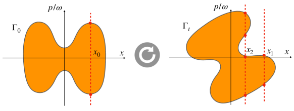
We now argue that the protocol introduced in Section I.2 can be described in terms of zero-entropy states, initially with two Fermi points ($Q=1$) and then at later times with four Fermi points ($Q=2$), see Fig. 1. Indeed, at initial time, the state of the system (in the large $N$ limit) is of the form (19), and the Fermi contour $\Gamma_{0}$ has a “butterfly-shape” (Fig. 1, left). Specifically, it reads

$$n(x,p,0)=\left\{\begin{array}[]{rcl}1&\quad{\rm if}\;|p|\leq\sqrt{2(\mu-V(x,0))},\\ 0&\quad{\rm otherwise}.\end{array}\right.$$ (24)

This means that locally it is parametrized by a single pair of Fermi points ($Q=1$). However, at time $t>0$ the evolution takes place within a harmonic trap $V(x,t>0)$. If $(x_{0},p_{0})$ is a given point of $\Gamma_{0}$, the corresponding point $(x_{t},p_{t})$ of the evolved contour $\Gamma_{t}$ at a given time $t$ is (cf. Eq. (23))

$$\begin{pmatrix}x_{t}\\ p_{t}/\omega\end{pmatrix}=\begin{pmatrix}\cos(\omega t)&\sin(\omega t)\\ -\sin(\omega t)&\cos(\omega t)\end{pmatrix}\begin{pmatrix}x_{0}\\ p_{0}/\omega\end{pmatrix},$$ (25)

meaning that, with the rescaling $p_{t}\rightarrow p_{t}/\omega$, $\Gamma_{t}$ simply rotates in phase space at the trap frequency $\omega$. [In contrast with the interacting case discussed in Ref. Ruggiero et al. (2020), $\Gamma_{t}$ is not deformed under time evolution.] Then, after some fraction of the period of the trap $\tau=2\pi/\omega$, a region appears near the center with a split Fermi sea, $Q=2$ (Fig. 1, right).

We stress that the appearance of multiple Fermi seas is a major difference with respect to the situations addressed in Refs. Ruggiero et al. (2019); Scopa et al. (2021). While there the hydrodynamic problem is equivalent to a conventional form of hydrodynamics, the protocol considered here (as well as in Ref. Ruggiero et al. (2020)) is the simplest generalization where GHD is really needed (see also Ref. Doyon et al. (2017)).

Figure 1: Left: Wigner function at initial time $t=0$. For any choice of $x_{0}$ the maximum number of Fermi points (intersections between the vertical line $x=x_{0}$ and the contour $\Gamma_{0}$) is two. Right: Evolved Wigner function according to Eq. (18): this corresponds to a simple rotation in the rescaled coordinates $(x,p/\omega)$ (cf. (25)). After time $t>0$ there are different regions, associated to a different number of Fermi points. For example, for a fluid cell around $x_{1}$ the number of Fermi points is still two. However, around $x_{2}$, there are four of them.

II.2 Quantum fluctuations around (non-interacting) Generalized Hydrodynamics

The goal of the theory of QGHD is to capture long-wavelength quantum fluctuations around the hydrodynamic solution of the GHD equation (18). This has been obtained in the free case in Ruggiero et al. (2019), and later generalized to truly interacting models in Ruggiero et al. (2020).

II.2.1 Propagation of quantum fluctuations

We now briefly recall the main steps for its derivation, restricting to the case of interest, namely the TG limit or, equivalently, non-interacting fermions. Starting from a zero-entropy hydrodynamic configuration (Eq. (19) or, equivalently, Eq. (20)), small fluctuations can be expressed as deformations of the contour Giamarchi (2003); Cazalilla (2004), meaning, locally, of the Fermi points, $p_{a}\to p_{a}+\delta p_{a}$. As shown in Ref. Ruggiero et al. (2020), $\{\delta p_{a}\}$ obey (at first order) the following equation

$$(\partial_{t}+p_{a}(x,t)\partial_{x})\delta p_{a}(x,t)=0,$$ (26)

describing the propagation of linear sound waves. Note that, as an important simplification occurring with respect to the interacting case, here the equations do not couple $p_{a},p_{b}$ with $a\neq b$. To make contact with Ref. Ruggiero et al. (2020), this follows from the fact that the flux jacobian $A_{a,b}\equiv\partial_{a}\epsilon/\partial p_{b}$ with $\epsilon_{a}=p_{a}(x,t)^{2}/2+V(x,t)$ denoting the semiclassical energy associated to $p_{a}$, is diagonal in this case (cf. Eq. (8) there).

One considers the quantized version of such fluctuations, obtained by viewing the small displacement of the contour $\delta p_{a}$ as an operator acting on a Hilbert space, $\delta p_{a}(x,t)\to\delta\hat{p}_{a}(x,t)$, $a=1,\dots,2Q$. A small displacement of the contour is equivalent to a small excess of particles around point $(x_{t},p_{t})$ in phase space, so we define the excess density operator as $\delta\hat{\rho}_{a}(x,t)=\frac{(-1)^{a}}{2\pi\hbar}\delta\hat{p}_{a}(x,t)$. Then, using the parameterization (22), it is more convenient to work with the excess density along the contour $\Gamma_{t}$, defined as

$$\delta\hat{\rho}(s,t)\equiv\left|\frac{dx_{t}(s)}{ds}\right|\delta\hat{\rho}_{a}(x_{t}(s),t),$$ (27)

for the index $a$ such that $p_{t}(s)=p_{a}(x_{t}(s),t)$. Here the Jacobian $|dx_{t}(s)/ds|$ is included because we want $\delta\hat{\rho}(s)$ to be a density along the contour; in particular we want

$$\delta\hat{N}\equiv\int_{0}^{2\pi}\delta\hat{\rho}(s)ds$$ (28)

to be the operator that measures the excess of particles in the gas with respect to the average number $N$. Notice that $\delta\hat{N}$ must have integer eigenvalues.

Next, we impose that the operator $\delta\hat{\rho}(s)$ satisfies the $\rm U(1)$ current algebra

$$[\delta\hat{\rho}(s),\delta\hat{\rho}(s^{\prime})]=\frac{1}{2\pi i}\delta^{\prime}(s-s^{\prime}),$$ (29)

so $\delta\hat{\rho}(s)$ is a chiral field that lives along the contour $\Gamma_{t}$. Note that instead of imposing the commutation relations of total densities and velocities, as in (7), we use the excess densities at different momenta, which are more natural variables in the QGHD context and lead to the commutation relations of a $\rm U(1)$ algebra. Locally, i.e., in a small cell around a fixed $x$, the above commutation relations are written in terms of several chiral components $\delta\hat{\rho}_{a}(x)$ (as many as the number of local Fermi points $p_{a}(x)$),

$$[\delta\hat{\rho}_{a}(x),\delta\hat{\rho}_{b}(y)]=\frac{(-1)^{a}}{2\pi i}\delta_{ab}\delta^{\prime}(x-y)\ .$$ (30)

The time-dependent Hamiltonian that generates the dynamics of the quantum fluctuations is Ruggiero et al. (2020)

$$\hat{H}[{\Gamma_{t}}]=\pi\hbar\sum_{a}\int dx\,(-1)^{a}{p_{a}(x,t)}\left({\delta\hat{\rho}_{a}(x)}\right)^{2}=\pi\hbar\int ds\,\left(\frac{dx_{t}(s)}{ds}\right)^{-1}{p_{t}(s)}\left(\delta\hat{\rho}(s)\right)^{2}.$$ (31)

This Hamiltonian depends on time only through its dependence on the contour $\Gamma_{t}$, and it is chosen so that it reproduces the evolution equation of sound waves (26). Indeed, plugging the Hamiltonian (31) into the Schrödinger equation for $\delta\hat{\rho}_{a}$, i.e. $\partial_{t}\delta\hat{\rho}_{a}(x)=\frac{i}{\hbar}\left[\hat{H}[\Gamma_{t}],\delta\hat{\rho}_{a}(x)\right]$, gives back the wave equation (26). Eq. (31) is a special case of the QGHD Hamiltonian given in Ruggiero et al. (2020) (for the Tonks-Girardeau gas, the flux Jacobian is $A_{a,b}=\delta_{ab}\,k_{a}$, see the comment above). For the Tonks-Girardeau gas, time-evolution under the Hamiltonian (31) simply induces a rotation of the field $\delta\hat{\rho}(s)$ together with the contour $\Gamma_{t}$. Indeed, the Heisenberg evolution equation for $\delta\hat{\rho}(s,t)$ reads (see Eq. (27))

$$\frac{d}{dt}\delta\hat{\rho}(s,t) = \left(\partial_{t}\left|\frac{dx_{t}(s)}{ds}\right|\right)\delta\hat{\rho}_{a}(x_{t}(s),t)+\left|\frac{dx_{t}}{ds}\right|(\partial_{t}x_{t}(s))\partial_{x}\delta\hat{\rho}_{a}(x_{t}(s),t)+\frac{i}{\hbar}[\hat{H}[\Gamma_{t}],\delta\hat{\rho}(s,t)]$$ (32)

$$= {\rm sign}\left(\frac{dx_{t}}{ds}\right)\frac{dp_{t}(s)}{ds}\delta\hat{\rho}_{a}(x_{t}(s),t)+\left|\frac{dx_{t}}{ds}\right|p_{t}(s)\partial_{x}\delta\hat{\rho}_{a}(x_{t}(s),t)+\frac{i}{\hbar}[\hat{H}[\Gamma_{t}],\delta\hat{\rho}(s,t)]$$

$$= {\rm sign}\left(\frac{dx_{t}}{ds}\right)\frac{dp_{t}(s)}{ds}\delta\hat{\rho}_{a}(x_{t}(s),t)+{\rm sign}\left(\frac{dx_{t}}{ds}\right)p_{t}(s)\partial_{s}\delta\hat{\rho}_{a}(x_{t}(s),t)+\frac{i}{\hbar}[\hat{H}[\Gamma_{t}],\delta\hat{\rho}(s,t)]$$

$$= \frac{\partial}{\partial s}\left(p_{t}(s)\left(\frac{dx_{t}}{ds}\right)^{-1}\delta\hat{\rho}(s,t)\right)+\frac{i}{\hbar}[\hat{H}[\Gamma_{t}],\delta\hat{\rho}(s,t)].$$

Note that the above derivation is done assuming to be far from the turning points (this means in particular that the ‘sign’ function is just a constant). We see that the first term is a convection term, which expresses the fact that the excess density is transported along the contour with a velocity $p_{t}(s)\left(\frac{dx_{t}}{ds}\right)^{-1}$. The second term is fixed by the Hamiltonian (31); in the general case of interacting theories, it is a non-trivial term, see Ruggiero et al. (2020). However, for the Tonks-Girardeau gas, it is easy to see from Eq. (31) that this term exactly compensates the convection term, so that

$$\frac{d}{dt}\delta\hat{\rho}(s,t)=0\ .$$ (33)

This is a consequence of $s$ being a co-moving coordinate in the evolution equation (23), and of the theory being non-interacting (no other terms come from the commutator, in contrast with the interacting case). Eq. (33) means that the evolution of the field is trivial, so that we only need to compute correlations at $t=0$ and the latter are then just “transported” in time according to (25) [in the general case the same would be “transported” according to GHD].

II.2.2 Quantum fluctuations and correlations at time $t=0$.

In the previous subsection, we have seen that quantum fluctuations propagate in a very simple way in the Tonks-Girardeau gas: they simply follow the motion of the contour $\Gamma_{t}$, as expressed by Eq. (33). If we know the correlation functions of the field $\delta\hat{\rho}(s)$ at time zero, then it is trivial to propagate them to later times thanks to Eq. (33).

To find correlation functions at time $t=0$, we observe that the system at $t=0$ must be in the ground state of the Hamiltonian $H[\Gamma_{0}]$. Notice that, so far, we have not made any specific choice of parameterization for the contour, see Eq. (22). All the equations we wrote so far were valid for an arbitrary parameterization. However, now it is useful to make the following choice, which greatly simplifies all calculations: we choose Dubail et al. (2017); Ruggiero et al. (2019)

$$s(x_{0})=\pi\frac{\int^{x_{0}}_{-R/2}dx/p(x,0)}{\int_{-R/2}^{R/2}dx/p(x,0)}\ ,$$ (34)

where $p(x,t)=\frac{1}{\pi}\sqrt{2(\mu-V(x,t))}$ and $[-R/2,R/2]$ is the interval where $V(x,0)<\mu$. This provides a coordinate $s\in[0,\pi]$ for the upper part of the Fermi contour at $t=0$, which can be continued to $s\in[\pi,2\pi]$ to parameterize also the lower part. With this choice, we have

$$\left(\frac{dx_{0}(s)}{ds}\right)^{-1}p_{0}(s)={\rm constant},$$ (35)

so that the Hamiltonian at time $t=0$ is simply

$$H[\Gamma_{0}]\propto\int_{0}^{2\pi}(\delta\hat{\rho}(s))^{2}ds.$$ (36)

We recognize the Hamiltonian of a chiral ${\rm U}(1)$ CFT on a circle of circumference $2\pi$. All correlation functions in that theory can be expressed in terms of the ones of the dimensionless bosonic field $\hat{\phi}(s)\in\mathbb{R}/(2\pi\mathbb{Z})$, defined such that

$$\delta\hat{\rho}(s)=\frac{1}{2\pi}\partial\hat{\phi}(s).$$ (37)

The operator $\hat{\phi}(s)$ satisfies the $\rm U(1)$ current algebra $[\partial\hat{\phi}(s),\partial\hat{\phi}(s^{\prime})]=-2\pi i\delta^{\prime}(s-s^{\prime})$ as a consequence of (29). The two-point function in the ground state of the quadratic Hamiltonian (36) is

$$\langle\hat{\phi}(s)\hat{\phi}(s^{\prime})\rangle=-\log\left|2\sin\frac{s-s^{\prime}}{2}\right|,$$ (38)

and all other correlation functions of primary operators in the theory can be obtained using Wick’s theorem. We stress that the fact that we have arrived at a CFT is specific to the GHD description of non-interacting particles Dubail et al. (2017); Ruggiero et al. (2019). As an important consequence, the (quadratic) theory of quantum fluctuations around GHD is complemented by conformal symmetry and leads to explicit results for correlation functions. In the interacting case, even though the theory is still quadratic, the Hamiltonian typically involves terms that break conformal invariance Brun and Dubail (2018); Granet et al. (2019); Gluza et al. (2021); Scopa et al. (2020) (we note that, even in the interacting case, there can exist peculiar situations where conformal invariance survives Collura et al. (2020)). In the general case, the two-point function (38) needs to be computed numerically, as the solution of a generalized Poisson equation Brun and Dubail (2018).

Finally, note that one needs to relate observables defined in the initial microscopic model to quantities in the theory. Specifically, a given observable $O(x,t)$ will take the form an expansion in series Brun and Dubail (2017, 2018)

$$\hat{O}(x,t)=\sum_{j}c_{j}\hat{\Phi}_{j}(x,t)$$ (39)

where, in our case, $\hat{\Phi}_{j}(x,t)$ are (conformally normalised) operators of a CFT that we can order according to their scaling dimension, and $c_{j}$ are non-universal constants, which in inhomogeneous and out-of-equilibrium settings, as the one we consider in this work, will further acquire a space and time dependence, i.e., $c_{j}\to c_{j}(x,t)$. The operators entering the expansion (39) are fixed by transformation under symmetries, dimension requirements, and so on (this was explicitly done, e.g., in Brun and Dubail (2018)).

Figure 2: Quantum quench from double to single well in the Tonks-Girardeau gas $\bar{g}\rightarrow\infty$. First row: Fermi contour. Second row: Absolute value of the connected density-density correlator. Last row: Entanglement entropy. Each row shows the corresponding quantity as a function of the spatial coordinate $x$, at different times, expressed as a fraction of the period $\tau$ (from $t=0$ in the first column to $t=0.60\tau$ in the last). Orange symbols are the numerical data (obtained from a lattice model in the dilute limit), whereas dashed blue lines are the QGHD predictions. The numerics for the density-density correlator shows large oscillations (cyan continuous line), therefore the analytic prediction is compared with its spatial averaging. It diverges at coinciding points as $x^{-2}$. The parameters are chosen as follows: system size $L=1200$; number of particles $N=66$; pre-quench potential $V(x,t=0)=a_{4}x^{4}-a_{2}x^{2}$ with $a_{4}=6/L^{4},a_{2}=1/L^{2}$ and $\mu=0.003$ for the chemical potential; post-quench potential $V(x,t>0)=\omega^{2}x^{2}/2$ with $\omega=1/L$ (and period $\tau=2\pi/\omega$).

III Results for the density fluctuations

In this section, we explicitly compute the leading asymptotic of the equal-time density-density (connected) correlation function, which cannot be predicted by GHD alone as Euler scaling gives simply zero (all correlations within different fluid cells vanish faster than the inverse distance).

Following the program outlined above, we first express the density operator $\hat{\rho}(x,t)$ in terms of operators in the CFT (31). Assuming to start with a zero-entropy state (cf. (20)), let $x$ and $t$ be such that the corresponding Wigner function $n(x,p,t)$ is associated with $Q$ Fermi seas. They can be traced back to their initial positions at $t=0$ via Eq. (25) so that, at initial time, they correspond to the $2Q$ points $\{s_{a}\}_{a=1,\cdots,2Q}$ on the initial contour $\Gamma_{0}$. Then, the claim is that $\hat{\rho}(x,t)$, at leading order, takes the form

$$\hat{\rho}(x,t)=\rho_{\rm GHD}(x,t)+\delta\hat{\rho}(x,t)+\cdots,\qquad\delta\hat{\rho}(x,t)\,=\,\sum_{a=1}^{2Q}\frac{1}{2\pi}\left(\frac{ds_{a}}{dx}\right)\partial\hat{\phi}(s_{a})$$ (40)

where $\rho_{\rm GHD}(x,t)=\int\frac{dp}{2\pi\hbar}\,n(x,p,t)$ is the particle density, and the ellipses denote further contributions coming from operators with higher scaling dimension (giving rise to subleading terms in the CFT). The operator $\delta\hat{\rho}$ measures the fluctuations of the particle density and we are interested in its two-point function at time $t$, namely,

$$\left<\delta\hat{\rho}(x,t)\delta\hat{\rho}(x^{\prime},t)\right>=\sum_{a,b=1}^{2Q}\frac{1}{(2\pi)^{2}}\left(\frac{ds_{a}}{dx}\right)\left(\frac{ds_{b}}{dx^{\prime}}\right)\langle\partial\phi(s_{a})\partial\phi(s_{b})\rangle\ .$$ (41)

Each correlator in the sum in the r.h.s. is readily determined: indeed it corresponds to the two point function of the primary field $\partial\hat{\phi}(s)$ in the ground state of the CFT (31), simply given by Di Francesco et al. (1997)

$$\langle\partial\hat{\phi}(s_{a})\partial\hat{\phi}(s_{b})\rangle=\frac{1}{\left|2\sin\frac{s_{a}-s_{b}}{2}\right|^{2}}.$$ (42)

In the specific protocol depicted in Section I.2, two regimes are expected: if, at time $t$, there are only two Fermi points at position $x$, then the sums in (41) stop at $Q=1$; if there are four Fermi points, then, it stops at $Q=2$. With this further prescription, Eq. (41) together with Eq. (42) is the final result.

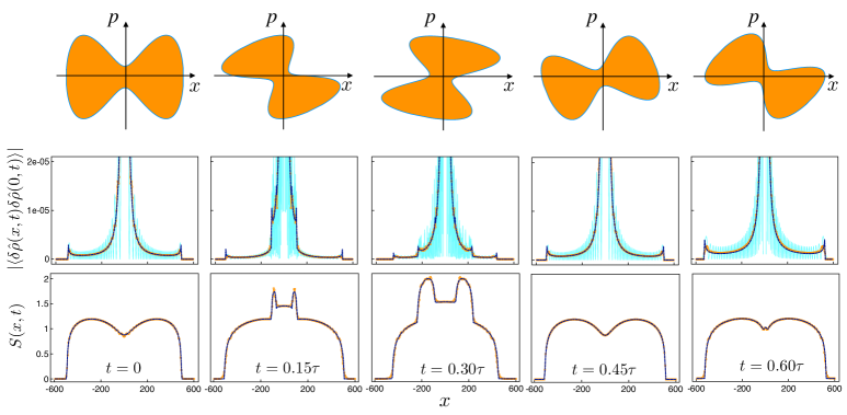
Our prediction is plotted in the second row of Fig. 2 and compared with exact numerics, which is achieved by taking advantage of the free fermionic nature of the TG limit (see Appendix A for details on the implementation) which makes it possible to consider large numbers of particles and long times. The exact microscopic solution has large Friedel oscillations (cyan curve) – coming from the presence of the trap, that breaks translational invariance Cazalilla (2002); Das et al. (2020); Artemenko et al. (2004) –, which can be suppressed by spatially averaging over a small window $[x-\Delta x/2,x+\Delta x/2]$. After averaging, the agreement with the prediction of QGHD is remarkable.

One interesting physical feature already noted in Ref. Ruggiero et al. (2020) is the divergence appearing at the points where a change in the number of Fermi points occurs, a genuine predictions of our theory. While in Ruggiero et al. (2020) such peaks were not visible in the microscopics of the interacting case, here (in the TG limit), instead, those are in fact visible also in the averaged microscopic simulations. Note that, in this case, we are able to get closer to the thermodynamic limit ($N=66$ in the Fig. 2 versus $N\leq 20$ in Ref. Ruggiero et al. (2020)), and therefore fluid cells are on smaller scale, so that peaks remain as meaningful non-microscopic features, beyond Euler cells.

IV Result for the entanglement entropy

In this section, we compute the entanglement entropy, as a function of space and time, for the protocol detailed in Section I.2. While it is known to vanish in GHD Alba (2019); Bertini et al. (2018); Alba et al. (2019), we are going to show that it is instead non-zero in QGHD. We also remind that this quantity is particularly challenging to compute directly within the microscopic model and therefore its calculation in this framework manifests the predictive power of our approach.

The entanglement entropy $S(x,t)$ between the subsystem $A=[-\infty,x]$ and its complement is defined as

$$S(x,t)=-\textrm{tr}\left(\sigma_{A}\ln\sigma_{A}\right)$$ (43)

where $\sigma_{A}$ is the reduced density matrix associated with $A$. In field theory, $S$ is usually obtained from the corresponding Rényi entropies $S_{\alpha}=\frac{1}{1-\alpha}\ln\textrm{tr}\left(\sigma_{A}^{\alpha}\right)$ (labelled by $\alpha\in\mathbb{R}$) via replica limit ($\alpha\to 1$). $S_{\alpha}$ can be expressed as the sum of two parts

$$S_{\alpha}(x,t)=\mathcal{S}_{\alpha}(x,t)-\epsilon(x,t).$$ (44)

Here $\mathcal{S}_{\alpha}(x,t)$ may be predicted by QGHD complemented with conformal invariance, whereas $\epsilon(x,t)$ is an ultraviolet cutoff. In the inhomogeneous situation, such cutoff also acquires a dependence on space and time Dubail et al. (2017).

The final result, that we are going to derive below, reads

$$S_{\alpha}(x,t)=-\frac{1}{12}\left(1+\frac{1}{\alpha}\right)\left\{\sum^{2Q}_{a>b}(-1)^{a+b}\ln\left|\left(p_{a}(x,t)-p_{b}(x,t)\right)\sin\frac{s_{a}-s_{b}}{2}\right|+\sum_{a}^{2Q}\ln\left|\frac{ds_{a}}{dx}\right|\right\}+\Phi_{\alpha}\ .$$ (45)

where, depending on the value of $x$ and $t$, $Q=1$ or $2$, and

$$\Phi_{\alpha}=\left(\Upsilon_{\alpha}+\frac{1}{6}\left(1+\frac{1}{\alpha}\right)\log 2\right)\times\frac{Q}{2}$$ (46)

is a non-universal constant, with $\Upsilon_{1}\simeq 0.4950179\dots$ for the von Neumann entropy ($\alpha=1$) and the expression for generic $\alpha$ can be found in Jin and Korepin (2004).

The comparison with numerics is shown in the last row of Fig. 2: the agreement is impressive.

IV.1 Universal contribution

Let us start with the derivation of the QGHD contribution. When $\alpha\in\mathbb{N}$, $\mathcal{S}_{\alpha}$ can be expressed as the correlation function of special fields known as twist fields Calabrese and Cardy (2004); Cardy et al. (2008); Calabrese and Cardy (2009), $\mathcal{T}$ and $\bar{\mathcal{T}}$, local operators lying at the boundary of the subsystem (in our case, the point $x$). Explicitly, we can write

$$\mathcal{S}_{\alpha}(x,t)=\frac{1}{1-\alpha}\ln\langle\mathcal{T}(x,t)\rangle.$$ (47)

In our chiral theory, twist fields are products of chiral excitations. We refer to them as chiral twist fields $\mathcal{\tau}$ and $\bar{\mathcal{\tau}}$. Crucially, in CFT, they behave as primary fields, with scaling dimension $\Delta=\frac{1}{24}\left(\alpha-\frac{1}{\alpha}\right)$ Calabrese and Cardy (2004). As in the previous example, two regimes are expected: if, at time $t$, there are only two Fermi points at position $x$, then $\langle\mathcal{T}(x,t)\rangle$ is a two-point function in the chiral CFT that lives along the Fermi contour; if there are four Fermi points $\langle\mathcal{T}(x,t)\rangle$ is a four-point function.

Let $x$ and $t$ be such that there are two Fermi point. Then, they can be traced back to their initial positions at $t=0$ via Eq. (25). Denoting the two initial coordinates along the Fermi contour by $s_{1},s_{2}$, Eq. (47) becomes

$$\mathcal{S}_{\alpha}=\frac{1}{1-\alpha}\ln\left(\left|\frac{ds_{1}}{dx}\right|^{\Delta}\left|\frac{ds_{2}}{dx}\right|^{\Delta}\langle\tau(s_{1})\bar{\tau}(s_{2})\rangle\right),$$ (48)

and

$$\langle\tau(s_{1})\bar{\tau}(s_{2})\rangle\simeq\frac{1}{\left|\sin\frac{s_{1}-s_{2}}{2}\right|^{2\Delta}}.$$ (49)

up to a normalization constant, giving rise to a subleading contribution in the final result (it can actually be computed as well, see Eq. (46)).

When at position $x$ and time $t$ we have four Fermi points, they can be traced back to positions $s_{1},s_{2},s_{3},s_{4}$ along the contour at time $t=0$. Then Eq. (47) becomes

$$\mathcal{S}_{\alpha}=\frac{1}{1-\alpha}\ln\left(\prod_{a=1}^{4}\left|\frac{ds_{a}}{dx}\right|^{\Delta}\langle\tau(s_{1})\bar{\tau}(s_{2})\tau(s_{3})\bar{\tau}(s_{4})\rangle\right),$$ (50)

where, similarly,

$$\langle\tau(s_{1})\bar{\tau}(s_{2})\tau(s_{3})\bar{\tau}(s_{4})\rangle\simeq\frac{\left|\sin\frac{s_{1}-s_{3}}{2}\right|^{2\Delta}\left|\sin\frac{s_{2}-s_{4}}{2}\right|^{2\Delta}}{\left|\sin\frac{s_{1}-s_{2}}{2}\right|^{2\Delta}\left|\sin\frac{s_{3}-s_{4}}{2}\right|^{2\Delta}\left|\sin\frac{s_{1}-s_{4}}{2}\right|^{2\Delta}\left|\sin\frac{s_{2}-s_{3}}{2}\right|^{2\Delta}}.$$ (51)

IV.2 Inhomogeneous cutoff and constant term via a generalized Fisher-Hartwig conjecture

The cutoff part $\epsilon(x,t)$ instead is not predicted by conformal invariance and has to be determined by other means, as well as the non-universal constant $\Phi_{\alpha}$ in (46). To do that, we start from a free fermionic model defined on a lattice and consider the continuous limit only at the end. Taking advantage of the free nature of the problem, we can rely on the Fisher-Hartwig conjecture Basor and Tracy (1991); Basor (1979); Jin and Korepin (2004); Calabrese and Essler (2010).

Let us start with a uniform system and consider the discrete version of a split Fermi sea, identified by a number of (adimensional) Fermi points $\{\kappa_{a}\}$. Those are related to their continuous analog $\{p_{a}\}$ by $p_{a}=\lim_{\delta\to 0}\kappa_{a}/\delta$, where $\delta$ is the lattice spacing. The cutoff is a function of them, that we denote as $\epsilon(\{\kappa_{a}\})$. The expression for two Fermi points is well-known Jin and Korepin (2004) and can be generalized to a generic number of Fermi seas.

The starting point is to write the entanglement entropy as the contour integral

$$S_{\alpha}=\frac{1}{2\pi i}\int_{\mathcal{C}}e_{\alpha}(\lambda)\frac{d\ln D(\lambda)}{d\lambda},$$ (52)

where $e_{\alpha}(x)=\frac{1}{1-\alpha}\log(x^{\alpha}+(1-x)^{\alpha})$ and $D(\lambda)=\det(\lambda-C_{A})$. $C_{A}$ is the correlation matrix of the subsystem $A$ in the split Fermi sea state and is a Toeplitz matrix. The symbol of such matrix in the case of multiple Fermi seas reads

$$g(\kappa)=\begin{cases}1\qquad\textrm{if}\;\kappa\in\;\textrm{Fermi seas,}\\ -1\quad\textrm{if}\;\kappa\not\in\;\textrm{Fermi seas.}\end{cases}$$ (53)

Hence the symbol defining $D(\lambda)$ is $\tilde{g}(\kappa)=\lambda-g(\kappa)$. If we consider $Q$ Fermi seas, such function has $2Q$ discontinuities, and can be represented as

$$\tilde{g}(\kappa)=\psi(\kappa)\prod_{a=1}^{2Q}t_{\beta_{i}(\lambda),\kappa_{a}}(\kappa),$$ (54)

where the points $\{\kappa_{a}\}$ correspond to the location of the discontinuities (i.e., the Fermi points), $\psi(\kappa)$ is the same as for a single Fermi sea Jin and Korepin (2004) and for $m\in\mathbb{N}$

$$\beta_{2m}(\lambda)=-\beta_{2m+1}(\lambda)=\beta(\lambda)\equiv\frac{1}{2\pi i}\ln\left(\frac{\lambda+1}{\lambda-1}\right),\quad t_{\beta_{a},\kappa_{a}}(\kappa)=\exp[-i\beta_{i}(\lambda)(\pi-\kappa+\kappa_{a})].$$ (55)

The Fisher-Hartwig conjecture provides the asymptotics of $D(\lambda)$. We are only interested in the additive constant (with respect to the subsystem size) part of $D(\lambda)$, which provides the cutoff. In particular, we consider the part of the constant term which depends on $\{\kappa_{a}\}$, omitting an overall function of $\lambda$. This is

$$\prod_{1\leq a\neq b\leq 2Q}\left(1-e^{i(\kappa_{a}-\kappa_{b})}\right)^{\beta_{a}\beta_{b}}.$$ (56)

The logarithmic derivative in (52) then gives

$$\frac{d}{d\lambda}\left[\sum_{a\neq b}\beta_{a}(\lambda)\beta_{b}(\lambda)\ln\left(1-e^{i(\kappa_{a}-\kappa_{b})}\right)\right]=\left(\frac{d\beta(\lambda)^{2}}{d\lambda}\right)\sum_{a\neq b}(-1)^{a+b}\ln(1-e^{i(\kappa_{a}-\kappa_{b})})=4\beta^{\prime}(\lambda)\beta(\lambda)\epsilon(\{\kappa_{a}\}),$$ (57)

where, in the last equality, we factorised the same expression appearing in the case of a single Fermi sea. Hence we can read off the cutoff as

$$\epsilon(\{\kappa_{a}\})=\frac{1}{12}\left(1+\frac{1}{\alpha}\right)\left[\frac{1}{2}\sum_{a\neq b}(-1)^{a+b}\ln\left(1-e^{i(\kappa_{a}-\kappa_{b})}\right)\right].$$ (58)

One can verify that Eq. (58) reduces to the known expressions in the case of a single Fermi sea Jin and Korepin (2004) and the case of many but symmetric Fermi seas Keating and Mezzadri (2005, 2004).

The continuous limit (in terms of $\{p_{a}\}$) is obtained by sending $\delta\to 0$ in (58), which gives

$$\epsilon(\{p_{a}\})\simeq\frac{1}{12}\left(1+\frac{1}{\alpha}\right)\sum_{a>b}(-1)^{a+b}\ln\left|{p_{a}-p_{b}}\right|$$ (59)

where we kept only the leading term, and we disregard a term proportional to $\ln\delta$. The latter, indeed does not enter in the final result (45) as it must be exactly compensated by a similar term in the universal contribution computed in Sec. IV.1. In fact, it is clear that in Eq. (48) or (50), in order to have dimensionless quantities inside the logarithm, the jacobians should be multiplied by a length scale (e.g., reasoning on the lattice, $\delta$).

For inhomogeneous systems, then, we just replace the Fermi points in (59) with the spacetime dependent ones $p_{a}\to p_{a}(x,t)$.

Finally, also the non-universal constant $\Phi_{\alpha}$ in (46) is similarly deduced from the result in the homogeneous model, still relying on the Fisher-Hartwig conjecture.

V Conclusions

This work is a follow-up of Ref. Ruggiero et al. (2020). We consider a 1d Bose gas undergoing the same quench dynamics as in Ruggiero et al. (2020), but focusing on the Tonks-Girardeau (infinite repulsion) limit. In this case, on the analytical side, more explicit results can be obtained by taking advantage of the restored conformal invariance. On the numerical side more stringent tests can be performed. In particular, analytical results are provided for the density fluctuations and the entanglement entropy after the quench, which are exact at the Euler scale, and systematically checked against numerics. For the entanglement entropy a non-universal space and time dependent contribution appears, which we are able to access by a generalization of the Fisher-Hartwig conjecture.

The theory introduced in Ref. Ruggiero et al. (2020) and further analysed in the present work has the potential to be applied to many out-of-equilibrium situation, as the one considered in this paper, and opens several further directions, also in connections with experiments.

A quantity of clear experimental interest is the one-particle density matrix, namely two-point correlation of the boson $\Psi$ entering the Lieb-Liniger Hamiltonian (11). This was obtained in Ruggiero et al. (2019) for a quench in a single-well potential, after a sudden change of the frequency. The extension of that analysis to the protocol studied here or, more generally speaking, in presence of multiple Fermi points, requires to work out the expression of $\Psi$ in terms of the CFT operators (cf. Eq. (39)), something that we plan to address in the near future. In the TG limit, this is something that would be experimentally accessible with modern setups such as the ones in Refs. Wilson et al. (2020); Malvania et al. (2020). The case of a finite interaction would be also interesting to investigate.

Moreover, we stress that the quantum GHD theory is defined when starting from zero-entropy states (cf. Eq. (19)). While they naturally arise in the thermodynamic limit of ground states of trapped bosons, this is not the case for thermal states, and how to extend the theory in this case is not straightforward. Indeed, by introducing a finite temperature, the Fermi contour entering the definition of zero-entropy Wigner functions gets smoothen, which in turn makes it difficult to clearly define chiral excitation around Fermi points. Still, this should be doable, at least at low temperature (similarly to what happens for standard Luttinger Liquid theory), and it would be interesting to study the interplay between thermal and quantum fluctuations.

A final point, mentioned in Section II, is that Eq. (18) for the evolution of the Wigner function is only valid at leading order when the potential $V(x,t)$ is not quadratic. Otherwise, corrections to that come as a series expansion in $1/\hbar$, also known as Moyal expansion Moyal (1949). Such corrections have been recently analyzed in great details Fagotti (2017, 2020) for free models, while for now it is not understood how to include them in truly interacting systems. We stress that they are different from the ones we are interested in, and in our case they are actually not there (the post-quench potential is quadratic). In general, however, the relation between the two needs to be clarified: eventually, taking into account the whole Moyal series should correspond to solving exactly the original microscopic model, thus including the ‘quantum’ effects we can describe with the quantum GHD approach.

Appendix A Details of the numerics

In order to simulate the Tonks-Girardeau limit of the Lieb-Liniger model (11), we consider its fermionic analog (14) and discretize it on a lattice. As well known, the procedure to go from a continuous to a discrete model is not unique. In our case, we focus on the following discretized quadratic Hamiltonian

$$H_{d}(t)=\sum_{i=1}^{L-1}J^{(1)}_{i}(c_{i}^{{\dagger}}c_{i+1}+c_{i+1}^{{\dagger}}c_{i})+\sum_{i=1}^{L-2}J^{(2)}_{i}(c_{i}^{{\dagger}}c_{i+2}+c_{i+2}^{{\dagger}}c_{i})+\sum_{i=1}^{L}V_{i}(t)c_{i}^{{\dagger}}c_{i}$$ (60)

which includes next-nearest neighbour hopping. Above, $c_{i}$ are spinless fermionic operators satisfying the canonical anticommutation relations $\{c_{i},c_{j}^{\dagger}\}=\delta_{ij}$. In (60) $L$ is the system size (that, due to the inhomogeneity, we need to keep finite to diagonalize the problem numerically), $J_{i}^{(1)}$ and $J_{i}^{(2)}$ are (inhomogeneous) hopping amplitudes, and $V_{i}(t)$ is the trapping potential. For our quench protocol, the latter is given by

$$V_{i}(t)=\begin{cases}a_{4}\left(i-L/2\right)^{2}-a_{2}\left(i-L/2\right)^{2}&t=0\\ \omega\left(i-L/2\right)^{2}&t>0\end{cases}\ .$$ (61)

For the simulations in Fig. 2 the parameters are fixed as follows: $J^{(1)}=-2/3,\,J^{(2)}=1/24,\,a_{4}=6/L^{4},\,a_{2}=1/L^{2},\omega=1/L$ and the chemical potential is fixed to $\mu=0.003$ (corresponding to $N=66$ particles in the ground state of the double well potential). We checked that, with this choice, the curves for the density profile after the quench looks perfectly periodic (namely, they are indistinguishable at $t=0$ and $t=\pi/\omega$).

To access the quantities of interest, we only need to diagonalize the two-point correlation function

$$C_{ij}(t)=\langle c_{i}^{{\dagger}}(t)c_{j}(t)\rangle\ ,$$ (62)

where $c_{i}^{({\dagger})}(t)=U^{{\dagger}}(t)c_{i}U(t)$ are the time evolved creation/annihilation operators (with $U(t)=e^{iH_{d}(t>0)t}$ the time-evolution operator).

Indeed, the state of the system is gaussian at all times, so that one can rely on Wick theorem Wick (1950) to compute the (connected) density-density correlations as

$$\langle\delta\rho_{i}(t)\delta\rho_{j}(t)\rangle=C_{ij}(t)(\delta_{ij}-C_{ji}(t))\ ,$$ (63)

where $\delta\rho_{i}(t)=\rho_{i}(t)-\langle\rho_{i}(t)\rangle$, and $\rho_{i}(t)=c_{i}^{{\dagger}}(t)c_{i}(t)$ is the local discrete density.

Moreover, for gaussian states, standard free fermions techniques can be used to compute the entanglement entropy Peschel et al. (1999); Peschel and Chung (1999); Chung and Peschel (2001); Peschel (2003, 2004); Peschel and Eisler (2009). Specifically, if for the subsystem $A=[-L,i]$ of the whole system, we define the two-point function restricted to $A$ with matrix elements $C^{A}_{ij}(t)=C_{ij}(t)$ for $i,j\in A$, and $\{\nu_{j}\}$ is its spectrum, then the entanglement entropy between $A$ and the rest (cf. Eq. (43)), is given by

$$S(i,t)=-\sum_{j}\left(\nu_{j}\log\nu_{j}+(1-\nu_{j})\log(1-\nu_{j})\right)\ .$$ (64)

The two-point function, in turn, can be computed via the following standard procedure. First, one needs to obtain the single-particle eigenstate amplitude of the pre-quench and post-quench Hamiltonian. By rewriting (60) as

$$H_{d}(t)=\sum_{ij}c_{i}^{{\dagger}}\,\mathbb{H}_{ij}(t)\,c_{j}\,$$ (65)

this is obtained by diagonalizing the $L\times L$ matrices $\mathbb{H}(t=0)$ and $\mathbb{H}(t>0)$, respectively. If we denote by $|\eta_{k}^{0}\rangle$ and $|\eta_{q}\rangle$, respectively, the eigenstates of such matrices, the two sets of corresponding eigenstates amplitudes are given by $\eta^{0}(k,i)\equiv\langle c_{i}|\eta^{0}_{k}\rangle$ and $\eta(q,i)\equiv\langle c_{i}|\eta_{q}\rangle$, with eigenvalues $\{\epsilon^{0}_{k}\}$ and $\{\epsilon_{q}\}$, for pre- and post-quench. $C_{ij}(t)$ is then expressed in terms of such quantities only. In fact, using the explicit form of the ground state of $\mathbb{H}(t=0)$

$$|\psi_{0}\rangle=\eta_{k_{N}}^{0\,{\dagger}}\eta_{k_{N-1}}^{0\,{\dagger}}\cdots\eta_{k_{1}}^{0\,{\dagger}}|0\rangle$$ (66)

with $|0\rangle$ the state annihilated by fermionic operators $\eta^{0}_{k}\,(\forall k)$ – those bringing $\mathbb{H}(t=0)$ in diagonal form –, and the decomposition

$$c_{i}(t)=\sum_{q}\eta(q,i)\,\eta_{q}(t),\quad\eta_{q}(t)=\eta_{q}\,e^{-i\epsilon_{q}t}$$ (67)

it can written as

$$C_{ij}(t)=\sum_{q,p=1}^{L}\sum_{l=1}^{N}e^{it(\epsilon_{q}-\epsilon_{p})}\,\eta^{*}(q,i)\,\eta(p,j)\,\alpha_{k_{l}}^{q}\alpha_{k_{l}}^{p\,*},\qquad\alpha_{k}^{q}\equiv\langle\eta^{0}_{k}|\eta_{q}\rangle=\sum_{n=1}^{L}\eta^{0\,*}(k,n)\,\eta(q,n)$$ (68)

which is straightforwardly implemented.

References

- Landau and Lifshitz (1987) L. Landau and E. Lifshitz, “Course of theoretical physics, vol. 6: Fluid mechanics 2, nd, ed,” (1987).
- Spohn (2012) H. Spohn, Large scale dynamics of interacting particles (Springer Science & Business Media, 2012).
- Abanov (2006) A. G. Abanov, in Applications of Random Matrices in Physics (Springer, 2006) pp. 139–161.
- Doyon et al. (2017) B. Doyon, J. Dubail, R. Konik, and T. Yoshimura, Phys. Rev. Lett. 119, 195301 (2017).
- Ruggiero et al. (2019) P. Ruggiero, Y. Brun, and J. Dubail, SciPost Phys. 6, 51 (2019).
- Landau et al. (1992) L. Landau, E. Lifshitz, R. Beyer, et al., in Perspectives in Theoretical Physics (Elsevier, 1992) pp. 359–361.
- Swift and Hohenberg (1977) J. Swift and P. C. Hohenberg, Physical Review A 15, 319 (1977).
- Forster (2018) D. Forster, Hydrodynamic fluctuations, broken symmetry, and correlation functions (CRC Press, 2018).
- Spohn (2014) H. Spohn, Journal of Statistical Physics 154, 1191 (2014).
- Landau (1941) L. Landau, Phys. Rev. 60, 356 (1941).
- Giamarchi (2003) T. Giamarchi, Quantum physics in one dimension, Vol. 121 (Clarendon press, 2003).
- Cazalilla (2004) M. Cazalilla, J. Phys. B 37, S1 (2004).
- Tsvelik (2007) A. M. Tsvelik, Quantum field theory in condensed matter physics (Cambridge university press, 2007).
- De Nardis et al. (2021) J. De Nardis, B. Doyon, M. Medenjak, and P. Miłosz, arXiv:2104.04462 (2021).
- Calabrese and Cardy (2004) P. Calabrese and J. Cardy, J. Stat. Mech. P06002 (2004).
- Calabrese and Cardy (2009) P. Calabrese and J. Cardy, J. Phys. A 42, 504005 (2009).
- Castro-Alvaredo et al. (2016) O. A. Castro-Alvaredo, B. Doyon, and T. Yoshimura, Phys. Rev. X 6, 041065 (2016).
- Bertini et al. (2016) B. Bertini, M. Collura, J. De Nardis, and M. Fagotti, Phys. Rev. Lett. 117, 207201 (2016).
- Ruggiero et al. (2020) P. Ruggiero, P. Calabrese, B. Doyon, and J. Dubail, Phys. Rev. Lett. 124, 140603 (2020).
- Alba et al. (2021) V. Alba, B. Bertini, M. Fagotti, L. Piroli, and P. Ruggiero, arXiv:2104.00656 (2021).
- Girardeau (1960) M. Girardeau, J. Math. Phys. 1, 516 (1960).
- Dean et al. (2018) D. S. Dean, P. Le Doussal, S. N. Majumdar, and G. Schehr, Phys. Rev. A 97, 063614 (2018).
- Dean et al. (2019) D. S. Dean, P. Le Doussal, S. N. Majumdar, and G. Schehr, EPL (Europhysics Letters) 126, 20006 (2019).
- Smith et al. (2020) N. R. Smith, D. S. Dean, P. Le Doussal, S. N. Majumdar, and G. Schehr, Physical Review A 101, 053602 (2020).
- Smith et al. (2021) N. R. Smith, P. L. Doussal, S. N. Majumdar, and G. Schehr, arXiv preprint arXiv:2106.05014 (2021).
- Lieb and Liniger (1963) E. H. Lieb and W. Liniger, Phys. Rev. 130, 1605 (1963).
- Berezin et al. (1964) F. Berezin, G. Pokhil, and V. Finkelberg, Vestnik MGU 1, 21 (1964).
- Korepin et al. (1997) V. E. Korepin, N. M. Bogoliubov, and A. G. Izergin, Quantum inverse scattering method and correlation functions, Vol. 3 (Cambridge university press, 1997).
- Kinoshita et al. (2004) T. Kinoshita, T. Wenger, and D. S. Weiss, Science 305, 1125 (2004).
- Kinoshita et al. (2006) T. Kinoshita, T. Wenger, and D. S. Weiss, Nature 440, 900 (2006).
- Wilson et al. (2020) J. M. Wilson, N. Malvania, Y. Le, Y. Zhang, M. Rigol, and D. S. Weiss, Science 367, 1461 (2020).
- Malvania et al. (2020) N. Malvania, Y. Zhang, Y. Le, J. Dubail, M. Rigol, and D. S. Weiss, arXiv preprint arXiv:2009.06651 (2020).
- Schemmer et al. (2019) M. Schemmer, I. Bouchoule, B. Doyon, and J. Dubail, Phys. Rev. Lett. 122, 090601 (2019).
- Scopa et al. (2021) S. Scopa, A. Krajenbrink, P. Calabrese, and J. Dubail, arXiv:2105.05054 (2021).
- Jin and Korepin (2004) B.-Q. Jin and V. E. Korepin, J. Stat. Phys. 116, 79 (2004).
- Keating and Mezzadri (2005) J. P. Keating and F. Mezzadri, Phys. Rev. Lett. 94, 050501 (2005).
- Keating and Mezzadri (2004) J. Keating and F. Mezzadri, Commun. Math. Phys. 252, 543 (2004).
- Wigner (1932) E. Wigner, Phys. Rev. 40, 749 (1932).
- Hillery et al. (1984) M. Hillery, R. F. O’Connell, M. O. Scully, and E. P. Wigner, Physics reports 106, 121 (1984).
- Cahill and Glauber (1969) K. E. Cahill and R. J. Glauber, Physical Review 177, 1882 (1969).
- Bettelheim et al. (2006) E. Bettelheim, A. G. Abanov, and P. Wiegmann, Phys. Rev. Lett. 97 (2006).
- Bettelheim et al. (2008) E. Bettelheim, A. G. Abanov, and P. B. Wiegmann, J. Phys. A 41, 392003 (2008).
- Bettelheim and Wiegmann (2011) E. Bettelheim and P. B. Wiegmann, Phys. Rev. B 84 (2011), 10.1103/physrevb.84.085102.
- Bettelheim and Glazman (2012) E. Bettelheim and L. Glazman, Phys. Rev. Lett. 109 (2012), 10.1103/physrevlett.109.260602.
- Protopopov et al. (2013) I. V. Protopopov, D. B. Gutman, P. Schmitteckert, and A. D. Mirlin, Phys. Rev. B 87, 045112 (2013).
- Moyal (1949) J. Moyal, Journal of the Royal Statistical Society. Series B (Methodological) 11, 150 (1949).
- Fagotti (2017) M. Fagotti, Phys. Rev. B 96, 220302 (2017).
- Fagotti (2020) M. Fagotti, SciPost Phys. 8, 48 (2020).
- Fokkema et al. (2014) T. Fokkema, I. Eliëns, and J.-S. Caux, Phys. Rev. A 89, 033637 (2014).
- Eliëns and Caux (2016) S. Eliëns and J.-S. Caux, J. Phys. A 49, 495203 (2016).
- Vlijm et al. (2016) R. Vlijm, S. Eliens, and J.-S. Caux, SciPost Phys. 1, 008 (2016).
- Eliëns (2017) I. S. Eliëns, On quantum seas, Ph.D. thesis (2017).
- Dubail et al. (2017) J. Dubail, J.-M. Stéphan, J. Viti, and P. Calabrese, SciPost Phys. 2, 002 (2017).
- Brun and Dubail (2018) Y. Brun and J. Dubail, SciPost Phys. 4, 037 (2018).
- Granet et al. (2019) E. Granet, L. Budzynski, J. Dubail, and J. L. Jacobsen, J. Stat. Mech. 2019, 013102 (2019).
- Gluza et al. (2021) M. Gluza, P. Moosavi, and S. Sotiriadis, arXiv:2104.07751 (2021).
- Scopa et al. (2020) S. Scopa, L. Piroli, and P. Calabrese, J. Stat. Mech. 2020, 093103 (2020).
- Collura et al. (2020) M. Collura, A. De Luca, P. Calabrese, and J. Dubail, Physical Review B 102, 180409 (2020).
- Brun and Dubail (2017) Y. Brun and J. Dubail, SciPost Phys. 2, 012 (2017).
- Di Francesco et al. (1997) P. Di Francesco, P. Mathieu, and D. Senechal, Conformal Field Theory (Springer, New York, USA, 1997).
- Cazalilla (2002) M. Cazalilla, EPL (Europhysics Letters) 59, 793 (2002).
- Das et al. (2020) J. P. Das, C. Chowdhury, and G. S. Setlur, Physica Scripta 95, 075710 (2020).
- Artemenko et al. (2004) S. N. Artemenko, G. Xianlong, and W. Wonneberger, Journal of Physics B: Atomic, Molecular and Optical Physics 37, S49 (2004).
- Schollwock (2011) U. Schollwock, Annals of Physics 326, 96 (2011).
- Alba (2019) V. Alba, Phys. Rev. B 99, 045150 (2019).
- Bertini et al. (2018) B. Bertini, M. Fagotti, L. Piroli, and P. Calabrese, J. Phys. A 51, 39LT01 (2018).
- Alba et al. (2019) V. Alba, B. Bertini, and M. Fagotti, SciPost Phys.. 7, 5 (2019).
- Cardy et al. (2008) J. Cardy, O. Castro-Alvaredo, and B. Doyon, J. Stat. Phys. 130, 129 (2008).
- Basor and Tracy (1991) E. L. Basor and C. A. Tracy, Physica A 177, 167 (1991).
- Basor (1979) E. L. Basor, Indiana Univ. Math. J. 28, 975 (1979).
- Calabrese and Essler (2010) P. Calabrese and F. H. L. Essler, J. Stat. Mech. P08029 (2010).
- Wick (1950) G. C. Wick, Phys. Rev. 80, 268 (1950).
- Peschel et al. (1999) I. Peschel, M. Kaulke, and O. Legeza, Annalen der Physik 8, 153–164 (1999).
- Peschel and Chung (1999) I. Peschel and M.-C. Chung, J. Phys. A 32, 8419–8428 (1999).
- Chung and Peschel (2001) M.-C. Chung and I. Peschel, Phys. Rev. B 64, 064412 (2001).
- Peschel (2003) I. Peschel, J. Phys. A 36, L205–L208 (2003).
- Peschel (2004) I. Peschel, J. Stat. Mech. 2004, P06004 (2004).
- Peschel and Eisler (2009) I. Peschel and V. Eisler, J. Phys. A 42, 504003 (2009).