The neutron-capture and $\alpha$-elements abundance ratios scatter in old stellar populations. Cosmological simulations of the stellar halo

Abstract

We investigate the origin of the abundance ratios and scatter of the neutron-capture elements Sr, Ba and Eu in the stellar halo of a Milky Way-mass galaxy formed in a hydrodynamical cosmological simulation, and compare them with those of $\alpha$ elements. For this, we implement a novel treatment for chemical enrichment of Type II supernovae which considers the effects of the rotation of massive stars on the chemical yields and differential enrichment according to the life-times of progenitor stars. We find that differential enrichment has a significant impact on the early enrichment of the interstellar medium which is translated into broader element ratio distributions, particularly in the case of the oldest, most metal-poor stars. We find that the [element/Fe] ratios of the $\alpha-$elements O, Mg and Si have systematically lower scatter compared to the neutron-capture elements ratios Sr, Ba and Eu at [Fe/H]$<-2$, which is $\sim 0.1-0.4$ dex for the former and between $\sim 0.5$ and $1$ dex for the latter. The different scatter levels found for the neutron-capture and $\alpha$-elements is consistent with observations of old stars in the Milky Way. Our model also predicts a high scatter for the [Sr/Ba] ratio, which results from the treatment of the fast-rotating stars and the dependence of the chemical yields on the metallicity, mass and rotational velocities. Such chemical patterns appear naturally if the different ejection times associated to stars of different mass are properly described, without the need to invoke for additional mixing mechanisms or a distinct treatment of the $\alpha-$ and neutron-capture elements.

1 Introduction

Thanks to the Gaia satellite which provides precise measurements of parallax and proper-motion of stars (Gaia Collaboration, Brown et al. 2021 and references therein), as well as spectroscopic information coming from major surveys (complementing the Gaia data with radial velocities and chemistry), the complexity of the formation history of our Galaxy has become evident. In particular, the local low-metallicity regime (below [Fe/H]$\sim-$0.8) turns out to be made of a collection of debris from past impacts with smaller galaxies (Helmi 2020 and references therein) as well as early in-situ formed stars (Miglio et al. 2021; Montalbán et al. 2021 - usually more enhanced in $\alpha$-elements).

The most important past accretion event in the early history of the Milky Way seems to have been the merger with Gaia-Enceladus (Helmi et al., 2018; Belokurov et al., 2018). This event could be confirmed thanks to the combination of Gaia DR2 (Gaia Collaboration, Brown et al., 2018) and APOGEE (Majewski et al., 2017) data. The discovery and characterization of other debris is a very active field and the several large spectroscopic surveys are playing a key role (e.g. Koppelman et al. 2019; Myeong et al. 2019; Naidu et al. 2020; Re Fiorentin et al. 2021). Indeed, the information brought by detailed chemical abundances is of paramount importance in the identification of a star’s origin.

The role of neutron-capture (n-capture) elements in this context is certainly going to be central as suggested by recent observational results (see for instance Aguado et al. 2021; Limberg et al. 2021; Gudin et al. 2021; Gull et al. 2021). In particular, the results of Ryan et al. (1996) and McWilliam (1998), later on confirmed by Honda et al. (2004) and François et al. (2007), showed that the [n-capture/Fe] ratios for metal-poor stars ([Fe/H]$<-2.5$) exhibit a large dispersion which can not be attributed to observational errors, although the scatter in their [$\alpha$/Fe] and [Fe-peak/Fe] ratios as functions of [Fe/H] is very small (Cayrel et al., 2004). This striking difference between the behaviour, at low metallicity, of neutron capture elements on one side and [$\alpha$/Fe] and [Fe-peak/Fe] ratios on the other hand, can be explained if the production of neutron capture elements by r-process is not homogeneous among the massive stars (Cescutti, 2008), as the production of the other elements. Another possibility is that the sites of r-process production were diverse and rare, such as electron capture SNe (Haynes & Kobayashi 2019, Cescutti et al. 2013), magneto-rotationally driven SNe (Cescutti & Chiappini, 2014), or neutron star mergers (Cescutti et al. 2015, Wehmeyer et al. 2015, Argast et al. 2004). Moreover, a dispersion is also present in the ratio [Sr/Ba] vs [Fe/H] at metallicity [Fe/H]$<-$2.5. This is usually attributed to the presence of a second neutron-capture process for the synthesis of the first-peak usually connected to a weak r-process (Busso et al., 1999; Qian & Wasserburg, 2000; Wanajo et al., 2001) and referred to as light elements primary production (LEPP) in Travaglio et al. (2004). Montes et al. (2007) showed that although weak r-process can play this role, the signature of an s-process from massive stars cannot be excluded.

The large spread in abundance ratios of n-capture elements is a consequence of the strong dependency of the stellar yields of these elements on the stellar mass and on different production channels (e.g. massive stars or neutron-star mergers). Hence, the study of the scatter among two different n-capture elements can bring important insights both on stellar nucleosynthesis and galaxy assembly (e.g. Cescutti et al. 2013; Cescutti & Chiappini 2014; Wehmeyer et al. 2015; Wehmeyer et al. 2019; Brauer et al. 2020; see also review by Cowan et al. 2021 and references therein). For example, Limberg et al. (2021) shows that the largest differences among accretion events are for n-capture elements and therefore these will be key to trace back the past accretion history of the Milky Way.

The fast observational progress in this area urgently calls for informative theoretical models which help the interpretation of chemo-kinematic datasets (with 6D phase space information plus chemistry and, sometimes, age - Valentini et al. 2019; Montalbán et al. 2021; Miglio et al. 2021).

The use of n-capture elements brings at least two important difficulties that have to be addressed before model predictions including these elements can become useful. The first is the uncertainties in the nucleosynthetic sites of production (in particular in the case of r-process elements, but also related to the early contribution of massive stars for the s-process - e.g. Choplin et al. 2018 and references therein). The second difficulty is related to the implementation of the evolution of these elements in cosmological simulations, and possible resolution/mixing effects that can affect their predictions (e.g. Shen et al. 2015; van de Voort et al. 2015; Naiman et al. 2018; Haynes & Kobayashi 2019; van de Voort et al. 2020). Most of these previous work consider only the production of elements by r-process events, either on-the-fly or in post-processing, or analyse the evolution of Eu only.

In this work, we implement a detailed chemical enrichment model which includes the production and distribution of Sr, Ba and Eu in a cosmological simulation. In particular, we explore the dispersion in light to heavy neutron-capture elements considering both r-process events and the contribution of massive stars with an s-process production (Frischknecht et al., 2016b; Limongi & Chieffi, 2018; Choplin et al., 2018). As summarized in Chiappini (2013), the impact of spinstars in the chemical enrichment of the earliest phases of our Galaxy is not confined to carbon and nitrogen (Chiappini et al., 2006; Chiappini et al., 2008; Prantzos et al., 2018), but extends to s-process elements as well (Pignatari et al., 2008; Chiappini et al., 2011). As a first step, in previous works we studied the scatter in n-capture abundance ratios using stochastic inhomogeneous chemical evolution models (Cescutti et al., 2013; Cescutti & Chiappini, 2014; Cescutti et al., 2015). Such models, by construction, do not include accretion of stars formed in smaller galaxies as we know to be the case in the Milky Way. In this work we investigate the impact of accretion events and the cosmological growth of halos on these previous results, in the context of the $\Lambda$-Cold Dark Matter model.

This paper is organized as follows. Sections 2 and 3 describe our new model for chemical enrichment and discuss the effects of differential enrichment on the predictions for the abundance ratios. Section 4 analyses the stellar halo formed in a cosmological simulation of a Milky Way-mass galaxy, focusing on the abundances and scatter of neutron-capture and $\alpha-$elements, and in Section 6 we present our conclusions.

2 The Simulations

2.1 Numerical Implementation

We employ for this study the cosmological, hydrodynamical, Smoothed Particle Hydrodynamics (SPH) code gadget3 (Springel et al., 2008), with the additional modules of Scannapieco et al. (2005, 2006) for describing star formation, chemical enrichment, supernova feedback, and metal-dependent cooling. For this project, we have modified our standard code, to which we refer to as the CS model, in order to properly describe the early enrichment phases of the interstellar medium, therefore allowing for a detailed study of the chemical abundances of the very old stars in galaxies. In the following subsections, we describe the CS model in terms of the physical modules relevant for this study, the updates we have implemented to the chemical routines, the chemical species and yields that we adopt, and the setup of the simulations presented in this work.

2.1.1 Star formation, feedback and chemical enrichment in the CS model

In the CS model, star particles form according to the Kennicutt-Schmidt law (Kennicutt, 1998), in a stochastic manner (Springel & Hernquist, 2003). Gas particles are eligible for star formation if they are denser than a critical value ($\rho_{\rm c}$) and are in a convergent flow. For these particles, the star formation rate (SFR) per unit volume is

$$\rho_{\rm SFR}=c_{*}{{\rho}\over{\tau_{\rm dyn}}}$$ (1)

where $c_{*}$ is a star formation efficiency, $\rho$ is the gas density and $\tau_{\rm dyn}=(4\pi G\rho)^{-1/2}$ the dynamical time of the particle. Once formed, star particles are treated as single stellar populations (SSP) with a given Initial Mass Function (IMF), and return metals and energy to their surroundings during supernova (SN) explosions. As the interstellar medium (ISM) gets polluted, new stars are produced with higher metallicities, because star particles inherit the element abundances of the gas from which they form. We assume that each gas particle can produce a maximum of two stars.

Our model includes treatments for chemical enrichment and energy feedback originated in Type II (SNII) and Type Ia (SNIa) events, based on assumptions for their rates, chemical yields and explosion times (Scannapieco et al., 2005), and the effects of stars in the AGB phase (Poulhazan et al., 2018). When a star experiences a SNII/SNIa/AGB event, the associated chemical production is distributed into its $N_{\rm Ngb}$ gas neighbours, in proportions given by the SPH kernel.

The CS model is based on a multiphase gas treatment which allows coexistence of dense and diffuse phases in the same spatial region; in this context, exploding stars will have well-defined hot and cold neighbours. We assume that both types of SNe eject the same amount of energy $E_{\rm SN}$ to the ISM, which is distributed in equal proportions to the local cold and hot gas phases of the exploding stars. Energy feedback into hot neighbors occurs at the time of explosion; however, for cold neighbors energy from successive explosions is instead accumulated and deposited only after a time-delay which depends on the local conditions of the cold and hot gas phases, as described in Scannapieco et al. (2006). In this way, artificial loss of SN energy in high-density regions is prevented. Gas cooling is described using the metal-dependent tables of Sutherland & Dopita (1993).

The CS model has been shown to be successful in producing galaxies similar to those observed, both in the case of Milky Way (MW) mass galaxies (Scannapieco et al., 2008, 2009, 2010, 2011; Tissera et al., 2013; Nuza et al., 2014; Tissera et al., 2014) and in dwarf systems (Sawala et al., 2010, 2011; Sawala et al., 2012). In particular, our SN feedback model is able to reproduce the formation of disks from cosmological initial conditions (Scannapieco et al., 2008, 2009), and to produce galaxies that are in general terms consistent with observations of the galaxy population (Scannapieco et al., 2012; Guidi et al., 2016).

2.1.2 Chemical species and yields of SNII

We consider in this work the nucleosynthesis of massive stars which end up their lives as Type II SNe, and that constitute the main drivers of the pollution of the ISM in the early phases of chemical evolution. In particular, we consider the nucleosynthesis of the following chemical species: H, He, C, N, O, Fe, Mg, Si, Ba, Eu, Sr and Y. The corresponding yields are parameterized in terms of $5$ metallicity ranges, separated by $Z=0$, $0.0001$ Z_⊙, $0.01$ Z_⊙, $0.1$ Z_⊙ and Z_⊙.

For He, C, N, O, Mg, Si and Fe, we have adopted the same nucleosynthesis than the ones used in Chiappini et al. (2006); Chiappini et al. (2008) and Cescutti & Chiappini (2010). In these works, the nucleosynthesis of He, C, N and O is metal-dependent and based on the work of the Geneve group (Meynet & Maeder, 2002; Hirschi, 2007). The novelty of this nucleosynthesis dataset is that the impact of rotation in massive stars at low metallicity is considered, and the rotation changes the final enrichment of the light elements, in particular of nitrogen. Unfortunately, the yields of the Geneve group could not be implemented for Mg, Si and Fe; in fact, Meynet & Maeder (2002) and Hirschi (2007) do not treat explosive nucleosynthesis, which has an important impact for these elements. Therefore, in this work, as well as in Chiappini et al. (2006); Chiappini et al. (2008) and Cescutti & Chiappini (2010), we use the solar metallicity yields from the work of Woosley & Weaver (1995), slightly modified (see François et al. 2004) to best match the averaged trend of extremely metal-poor stars measured by Cayrel et al. (2004). For Fe, the prescriptions are similar, with the exception of the zero metallicity table, where the population III stars with masses above $20$M_⊙ inject negligible amounts of iron into the ISM upon their death (Cescutti & Chiappini, 2010). Since Mg, Si and Fe are primary elements, the use of the solar metallicity table is a safe assumption.

For the nucleosynthesis of the neutron capture elements, we assume an r-process contribution as the one adopted in Cescutti et al. (2013): a strong production in a narrow mass range of $8-10$M_⊙ that we call standard r-process site. These yields have been chosen to reproduce the mean trend of [Ba/Fe] versus [Fe/H] using the homogeneous chemical evolution model of Chiappini et al. (2006). For the remaining neutron capture elements, we scale the r-process contribution using the ratios observed in r-process rich stars (Sneden et al., 2008). We also adopt an s-process contribution coming from rotating massive stars, using the yields computed in Frischknecht et al. (2016a). Among the set of models, we have adopted a robust production of s-process elements, achieved by considering s-process yields of massive stars for $v_{\rm ini}/v_{\rm crit}=0.5$ (fast rotators) and for a reaction rate ¹⁷O$(\alpha,\gamma)^{21}$Ne one tenth of Caughlan & Fowler (1988); current uncertainties on this rate are still large.

The stellar yields adopted here are essentially the same as the ones adopted in our non-cosmological stochastic model presented in Cescutti & Chiappini (2014). Using similar prescriptions, now applied to cosmological simulations, allows to test the impact of complex merger histories on the interpretation of the observed abundance scatter of different chemical elements, which is one of the main goals of the present work.

Throughout this paper, we have assumed the solar abundances given by Grevesse et al. (2010).

2.1.3 Implementing multiple explosion times for SNII

In the CS model, each star particle explodes as SNII in a single event, ejecting the whole chemical production of the SSP it represents at the time of the explosion. This time is determined by the mean age of the individual stars of the SSP. This assumption allows to describe the overall evolution of chemical abundances in galaxies; however, it does not properly describe the first stages of enrichment of the ISM, which will be enriched gradually, starting with the most massive, most short-lived stars. Such a gradual enrichment will leave imprints in the chemical properties of the very old, metal-poor stars, as stars of different mass will contribute chemical material of different nature (e.g. end-products of r- vs s-processes vs $\alpha$-elements) at different times. It will also significantly affect the spread in chemical abundances, which we investigate in this work.

In order to better describe the enrichment of the ISM occurring in short time-scales, we have modified our code such that each SNII event is represented by a series of different “explosions”, which we chose to best describe the enrichment of the different chemical elements we are interested in. In particular, we assume that each star particle will experience 5 different explosion events, which occur at 30, 18, 9, 6 and 3 Myr from its formation. These correspond to stars in the mass ranges [8-9), [9,14), [14, 27.5), [27.5, 45) and [45-100] M_⊙, respectively, according to the estimations of Maeder & Meynet (1989). The choice of $5$ explosion events per star particle allows to properly describe the differential enrichment produced by the individual stars, in terms of the chemical species and yields used in this work, avoiding large numerical overcosts.

2.1.4 Simulation set-up

We have tested our code in idealized simulations of the evolution of an isolated galaxy, as well as in simulations in a cosmological context. In order to facilitate comparison, we have kept the same input parameters for star formation, chemical enrichment and feedback in all runs, and performed simulations with the CS standard code and with the new implementation. We have assumed a star formation efficiency of $c_{*}=0.1$, a star formation threshold of $\rho_{\rm c}=0.1$ cm^-3, and $E_{\rm SN}=0.7\times 10^{51}$ erg of energy per SN. For the number of neighbours assumed for the SPH calculations, we used $N_{\rm Ngb}=40$. These choices for the input parameters produce galaxies with realistic disk sizes (Scannapieco et al., 2008). In order to facilitate comparison with the results of the galactic chemical evolution models of Cescutti et al. (2013), we have assumed a Scalo IMF.

All simulations presented in this paper have been run with the modules for SNIa and AGB stars switched off. The reason for this choice is to properly identify and isolate the effects of the fast-rotating stars and of considering differential enrichment on the chemical abundance ratios and scatter of $\alpha-$ and n-capture-elements. Note that we focus our analysis on the stellar halo component, which is formed by very old stars and therefore whose abundances are almost exclusively determined by the very early enrichment produced by SNII explosions. In future papers, we will explore the impact of SNIa and AGBs in the chemical enrichment histories, but this is beyond the scope of the present work.

3 The effects of differential SNII enrichment

In this Section we discuss the effects of implementing progressive enrichment via SNII on the chemical abundances and scatter of the gas and stellar components of galaxies. In particular, we compare simulations where the individual stars that are represented in a stellar particle explode simultaneously or progressively, better describing the first enrichment epochs. We refer to these two cases, correspondingly, as the single explosion (SE) or multiple explosion (ME) models. In SE we assume that each star particle formed in the simulation ejects all its chemical production in a single event (i.e. as in the standard CS model). In contrast, model ME assumes a progressive enrichment, in which the individual stars explode at different times, according to their masses and typical time-scales, as explained in Section 2.1.3.

In the following we compare the predictions of two simulations of the formation of a Milky Way-mass galaxy in an idealized, isolated scenario, that assume the SE and ME models. We refer to them as the “SE64” and “ME64” runs, respectively. Table 1 summarizes the main properties of these simulations, as well as those of additional simulations that we run in order to test possible dependencies of our results on numerical choices. These include simulations varying the number of particles (discussed in Appendix A.1), as well as the number of SPH neighbours ($N_{\rm Ngb}$, which sets the smoothing region, i.e. the radius over which the chemical elements ejected in SN explosions are distributed (discussed in Appendix A.2).

Table 1: Main characteristics of the simulations used in this work: reference name, type of initial conditions, number of SNII explosion events assumed ($N_{\rm SNII}$), total number of particles of the simulation ($N_{\rm tot}$), assumed number of SPH neighbours ($N_{\rm Ngb}$), reference Section, and masses of the dark matter ($m_{\rm DM}$) and baryonic ($m_{\rm bar}$) particles.

Name	Initial Conditions	$N_{\rm SNII}$	$N_{\rm tot}^{1}$	$N_{\rm Ngb}$	Section	$m_{\rm DM}$ [M⊙]	$m_{\rm bar}$ [M⊙]
SE64	Isolated	1	$2\times 64^{3}$	40	3	$6.55\times 10^{6}$	$7.28\times 10^{5}$
ME64	Isolated	5	$2\times 64^{3}$	40	3	$6.55\times 10^{6}$	$7.28\times 10^{5}$
SE64-NNgb64	Isolated	1	$2\times 64^{3}$	64	A.2	$6.55\times 10^{6}$	$7.28\times 10^{5}$
ME64-NNgb64	Isolated	5	$2\times 64^{3}$	64	A.2	$6.55\times 10^{6}$	$7.28\times 10^{5}$
SE64-NNgb128	Isolated	1	$2\times 64^{3}$	128	A.2	$6.55\times 10^{6}$	$7.28\times 10^{5}$
ME64-NNgb128	Isolated	5	$2\times 64^{3}$	128	A.2	$6.55\times 10^{6}$	$7.28\times 10^{5}$
SE32	Isolated	1	$2\times 32^{3}$	40	A.1	$5.22\times 10^{7}$	$5.80\times 10^{6}$
ME32	Isolated	5	$2\times 32^{3}$	40	A.1	$5.22\times 10^{7}$	$5.80\times 10^{6}$
SE32-NNgb64	Isolated	1	$2\times 32^{3}$	64	A.2	$5.22\times 10^{7}$	$5.80\times 10^{6}$
ME32-NNgb64	Isolated	5	$2\times 32^{3}$	64	A.2	$5.22\times 10^{7}$	$5.80\times 10^{6}$
SE32-NNgb128	Isolated	1	$2\times 32^{3}$	128	A.2	$5.22\times 10^{7}$	$5.80\times 10^{6}$
ME32-NNgb128	Isolated	5	$2\times 32^{3}$	128	A.2	$5.22\times 10^{7}$	$5.80\times 10^{6}$
SE128	Isolated	1	$2\times 128^{3}$	40	A.1	$8.19\times 10^{5}$	$9.10\times 10^{4}$
ME128	Isolated	5	$2\times 128^{3}$	40	A.1	$8.19\times 10^{5}$	$9.10\times 10^{4}$
SE128-NNgb64	Isolated	1	$2\times 128^{3}$	64	A.2	$8.19\times 10^{5}$	$9.10\times 10^{4}$
ME128-NNgb64	Isolated	5	$2\times 128^{3}$	64	A.2	$8.19\times 10^{5}$	$9.10\times 10^{4}$
SE128-NNgb128	Isolated	1	$2\times 128^{3}$	128	A.2	$8.19\times 10^{5}$	$9.10\times 10^{4}$
ME128-NNgb128	Isolated	5	$2\times 128^{3}$	128	A.2	$8.19\times 10^{5}$	$9.10\times 10^{4}$
SE	Cosmological	1	1854223	40	B	$2.16\times 10^{6}$	$4.11\times 10^{5}$
ME	Cosmological	5	1608991	40	B	$2.16\times 10^{6}$	$4.11\times 10^{5}$

¹ In the case of the cosmological simulations $N_{\rm tot}$ refers to the total number of particles within the virial radius of the galaxy at the end of the simulation ($z=0$).

The initial conditions are generated by radially perturbing a spherical grid of superposed dark matter and gas particles to produce a cloud with density profile $\rho(r)\sim r^{-1}$, as in Navarro & White (1993). The sphere is initially in solid body rotation with an angular momentum characterized by spin parameter $\lambda\simeq 0.1$, and the gas is cold (i.e. the initial thermal energy is only $5$ per cent of its binding energy). The simulated system has a total mass of $10^{12}\,{\rm M}_{\odot}$, 10 per cent of which is in the form of baryons, and the initial radius is $100\,{\rm kpc}$. Our fiducidal tests used $N_{\rm tot}=2\times 64^{3}$ particles initially, yielding particle masses of $6.55\times 10^{6}$ M_⊙ and $7.28\times 10^{5}$ M_⊙ for dark matter and gas (Table 1), respectively, and we adopted a gravitational softening length of $350$ pc for all particles. The simulations of this Section were run for 2 Gyr, although we focus our analysis on the early phases of the formation of the galaxies, before the first Gyr of evolution.

We note that the idealized initial conditions of this Section yield a simple model for disc formation, which is an ideal test bench for the performance and validity of the code. However, these models are not meant to provide a realistic scenario for the whole galaxy formation process, in particular because there is no gas infall which, in a cosmological context, has important effects on the growth and evolution of a galaxy. As explained above, we have also tested our model on cosmological simulations (see Appendix B).

3.1 Effects on the chemical enrichment of the ISM

Our implementation of multiple events per SN explosion is expected to affect not only the chemical properties of the galaxies but also the star formation process, as the rate at which the gas is enriched will impact the cooling rates, affecting the amount of cold/dense gas available for star formation at different times. This will produce an initial change in the star formation rate due to variations in the enrichment level, and further changes due to the variations in the amount of available feedback.

Fig. 1 shows the star formation rate (SFR), and the evolution of the stellar mass ($M_{\rm star}$) and stellar metallicity (Z, defined as the mass in metals – all chemical elements except hydrogen and helium – divided by the total mass) in simulations SE64 and ME64. The two simulations have similar SFRs and integrated stellar masses during the first $\sim 0.5$ Gyr; however, the metallicity of the stellar population is clearly distinct from very early times. This difference originates in the variations of the enrichment of the ISM in the two runs: in ME64 the first explosion events associated to the most massive short-lived stars occur very quickly after star formation (i.e. $3$ Myr, Section 2.1.3) triggering a very fast enrichment of the surrounding gas. In contrast, in SE64 the single explosion associated to all SNII within a star particle occurs after $\sim 15-20$ Myr from its formation.

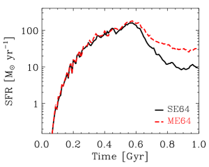
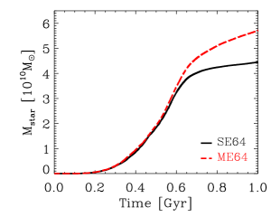
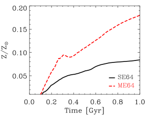
Figure 1: Star formation rate, cumulative stellar mass and stellar metallicity, as a function of time, for our simulations SE64 and ME64.

The differences in the early chemical pollution of the ISM in our two simulations can be seen in Fig. 2, where we compare the gas metallicities, in terms of the [Fe/H] abundance, for simulations SE64 and ME64, and for various times between $0.1$ and $0.35$ Gyr. Even though star formation starts at the same time in both simulations, in ME64 the enrichment of the ISM is faster compared to SE64, particularly during the first 200 Myr after star formation begins. At later times, the differences dilute, as both the $5$ explosion events in ME64 and the single event in SE64 have occurred, and the accumulated chemical production has been released. As a result, the predicted number of very metal-poor stars formed within the first 200 Myr when considering the multi-explosion scenario is systematically smaller in ME64, compared to those obtained when assuming that all core-collapse SNe contributed at a single time.

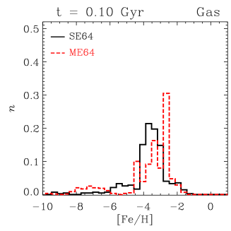
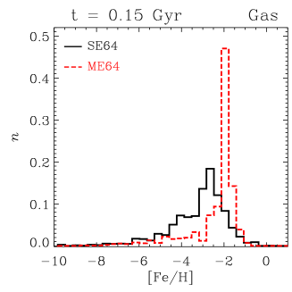
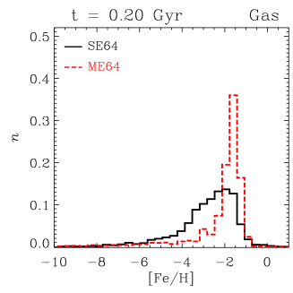
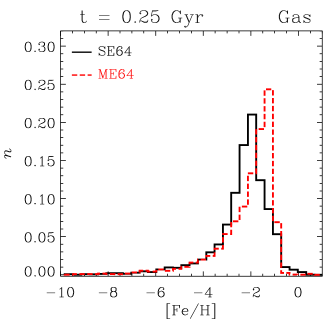
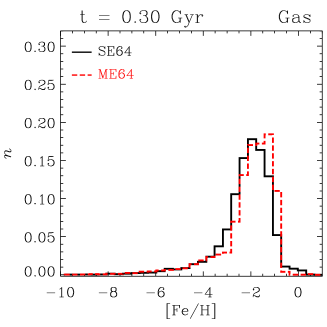
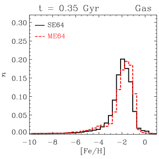
Figure 2: Distribution of [Fe/H] for the gas in simulations SE64 and ME64, for various times during the early enrichment phases.

The differences in the very early epochs, can thus leave clear imprints in the galaxies, both in the enrichment levels of the stellar and gaseous components (higher stellar metallicities in ME64 compared to SE64) and in the cooling rates (enhanced cooling in ME64 due to the faster enrichment). As a result, the star formation rates in ME64 are higher compared to SE64 and, after 1 Gyr of evolution, the stellar mass is higher ($\sim 30\%$) in ME compared to SE64, and the stellar metallicity in ME64 is about 2 times higher (Fig. 1).

Fig. 3 shows the distribution functions of stellar [Fe/H] abundances for simulations SE64 and ME64, after $0.25$, $0.5$ and $1$ Gyr of evolution. From these plots we can observe that, following the characteristics of the ISM enrichment, the differences in the [Fe/H] distributions in models SE64 and ME64 are more important at early times, both for low and high metallicity. The distributions are less dissimilar at later times; however, the differences originated early on on the stellar abundances can still be seen after 1 Gyr of evolution.

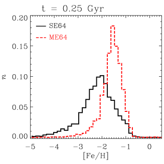
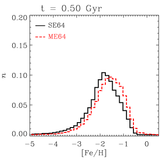
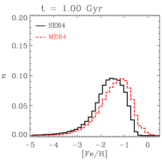
Figure 3: Distribution of the stellar [Fe/H] for simulations SE64 and M64 at different times of the simulation: 0.25 Gyr, 0.5 Gyr and 1 Gyr.

As explained above, imprints of the differences in the early chemical pollution of the ISM in runs SE64 and ME64 appear in the chemical properties of the stars. This is important given that, if properly interpreted, observations of the stellar population of a galaxy could allow to reconstruct the level of enrichment of the ISM at different times, information that is otherwise inaccessible.

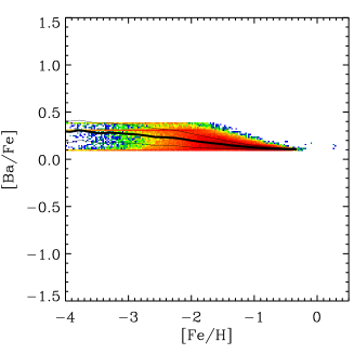
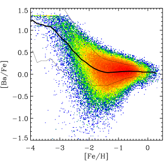
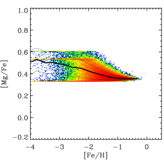
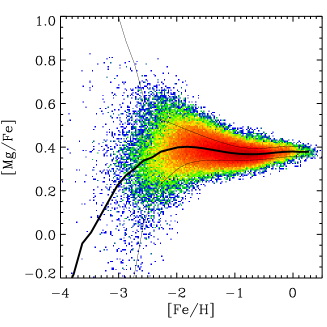
Figure 4: Element ratios of the neutron-capture element Ba and the $\alpha-$element Mg, in simulations SE64 (left-hand panels) and ME64 (middle-hand panels), after 1 Gyr of evolution. The solid thick and thin lines show, correspondingly, the median and 1$-\sigma$ levels. The colour scale is also shown.

3.2 Effects on the abundance ratios and their scatter

In this Section we focus on the element ratios of various chemical species, and the variations originated in simulations considering a single or multiple explosion events per SNII. In all cases, we analyse the distributions after 1 Gyr of evolution; as we have shown above, at this time differences in simulations SE64 and ME64 have already appeared but the variations in SFRs and total stellar masses are still moderate, allowing to better isolate the effects of assuming single or multiple explosion events per SN from the feedback effects that follow variations in the SFRs. Furthermore, this choice will allow a simpler comparison with the results of our cosmological simulations of Appendix B.

We show in Fig. 4 the distributions of stellar [Ba/Fe] as a function of [Fe/H] in simulations SE64 and ME64, after 1 Gyr of evolution (the behaviour of the other n-capture elements, Eu and Sr, are similar). We also show the corresponding median values (thick lines) and the $\pm\sigma$ levels (thin lines). Clearly, the implementation of multiple explosion times (ME64) has a strong impact in the predicted abundance ratios, particularly in the case of the metal-poor stars with [Fe/H] $<\kern-11.99998pt\lower 4.73611pt\hbox{$\sim$}~{}-1$. For [Fe/H] $\gtrsim-1$, the mean abundance ratios of stars in the two runs is similar, although the scatter in ME64 is higher. For metal-poor stars the differences between SE64 and ME64 are dramatic, not only in terms of their median values, but more importantly in terms of scatter. If a single SNII explosion event is assumed, as in SE64, the abundance ratios are limited to a narrow range determined by the IMF weighted mean of the stellar yields. In this simulation, the spread in the abundance ratios of [Ba/Fe] of the order of $0.3$ at the most, for all metallicities. In contrast, the abundance ratio of stars in ME64 show not only a much larger scatter up to $2$ dex, but also a clear relation between the scatter and the metallicity, such that the scatter decreases with increasing metallicity (a behaviour that extends towards stars with higher abundances). Stars in ME64 have a large variety of possible element ratios, even for coeval stellar populations, which results from the dependence of the chemical yields primarily on the stellar mass, but also on metallicity.

An important observation from this figure is that the lowest and highest abundance ratios that are found in ME64 can not be described in SE64; in fact, in ME64 a significant fraction of the stars is in the range of abundance ratios that are absent in SE64.

Now we turn our focus to the $\alpha$-elements, showing in the lower panel of Fig. 4 the distribution of [Mg/Fe], which we use as an example for this type of element (Si and O exhibit similar trends). In general terms, the behaviour of the $\alpha-$elements is similar to that observed for the neutron-captures elements, in the sense that simulation ME64 allows the abundance ratios to vary more compared to SE64, producing more realistic abundance patterns. Furthermore, we can see, in ME64, a positive and strong correlation between [Mg/Fe] and [Fe/H], which is, particularly for metal-poor stars, opposite to that found in SE64. Similarly to our findings for the neutron-capture elements, for the $\alpha$-elements we find that in ME64 the spread in abundance ratios decreases with increasing metallicity. It is important to note that, in our simulation ME64, the abundance ratios of neutron-capture elements extend over 3 dex while a smaller spread (or around 1 dex) is predicted for the $\alpha-$ elements.

The results of this Section show that a correct description of the different ejection-times of release of chemical elements of different mass stars contributing as core-collapse SNe is important in order to properly describe the early enrichment phases of the ISM in galaxies, and the abundances and scatter of the very metal-poor stars. We have shown the effects of differential enrichment using isolated simulations, but the same results are reproduced in cosmological runs, in terms of the changes in abundance ratios and scatter (see Appendix B) although with a higher level of complexity due to the cosmological evolution.

4 Abundances and scatter in the stellar halo

In this Section we study the chemical properties of the stellar halo formed in a cosmological simulation of the formation of a Milky Way-mass galaxy. This simulation, referred to as the ME run, assumes multiple explosion times per SNII.

The initial conditions used for our cosmological simulations correspond to halo named Aq-C of the Aquarius Project (Springel et al., 2008). The simulated halo has, at $z=0$, a virial mass of $1.6\times 10^{12}$ M_⊙ (see Table 1), a virial radius of $170$ kpc and is, by design, mildly isolated (no neighbour exceeding half its mass within a sphere of 2 Mpc radius). The simulations start at $z=127$ and run until $z=0$.

The ICs are consistent with a $\Lambda$-Cold Dark Matter universe with the following cosmological parameters: $\Omega_{\rm m}=0.25$, $\Omega_{\Lambda}=0.75$, $\Omega_{\rm b}=0.04$, $\sigma_{8}=0.9$ and $\text{H}_{0}=100\,h\,\text{km}\text{ s}^{-1}\text{Mpc}^{-1}$, with $h=0.73$. The mass resolution is $4.1\times 10^{5}$M_⊙ and $2.2\times 10^{6}$M_⊙ for gas and dark matter particles, respectively, and we have adopted a gravitational softening of 700 pc, fixed in comoving coordinates. The input parameters used for these simulations are the same than those used in the idealized simulations of the previous Section, in order to facilitate comparison.

Fig. 5 shows the face-on and edge-on projections of the stellar mass density (left-hand panels) at $z=0$ for the simulated galaxy, together with the corresponding metallicity distributions (right-hand panels). In order to make the projections, we have aligned the total angular momentum of the stars with the $z$ direction. The simulated galaxy is, at the present time, composed of a compact, dispersion-dominated bulge and a rotationally-supported disk. The rotation of the disks is clearly seen, particularly in the face-on view, from the velocity field included in this figure. The stellar halo is spatially extended, and significantly fainter than the other stellar components. The metallicity distributions reveal the different levels of enrichment in the different stellar components, the bulge and disc being significantly more enriched than the stellar halo region.

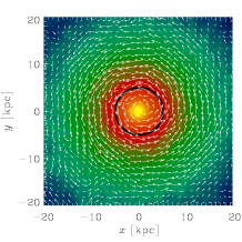
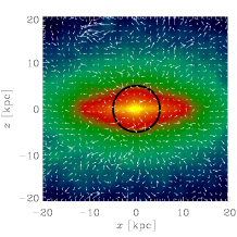
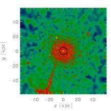
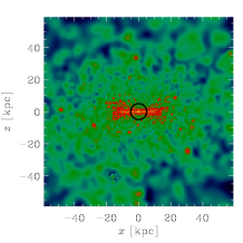
Figure 5: Maps of projected stellar mass density (left-hand panels) and stellar metallicity (right-hand panels) for the simulated galaxy in our cosmological simulation ME, at $z=0$, in face-on ($xy$) and edge-on ($xz$) views. The white arrows in the mass density maps indicate the corresponding velocity fields and reveal that, at the present time, the simulated galaxy has a rotationally-supported disk-like component, a compact bulge, and an extended stellar halo.

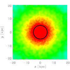
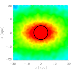
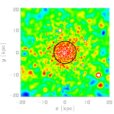
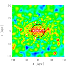
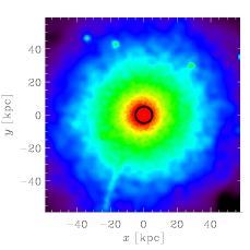
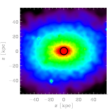
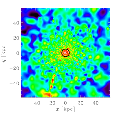
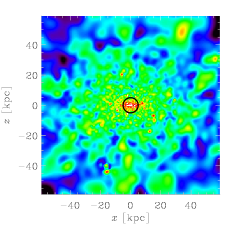
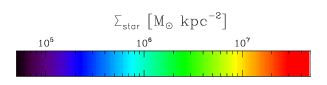
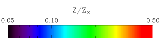
Figure 6: Maps of projected stellar mass density (left-hand panels) and stellar metallicity (right-hand panels), at $z=0$, for our cosmological simulation ME, considering stars that formed in the first Gyr of evolution. In both cases we show two perpendicular projections, corresponding to the face-on and edge-on projections of Fig. 5. The black circle shows our threshold of 5 kpc to define halo stars. The upper- and lower panels show, respectively, the inner galaxy and a zoom-out up to 0.25 of the virial radius. Note that the colour code and scale have been chosen in order to highlight the halo density and metallicity structure (note that these are different from those used in Fig. 5).

In order to study the abundances in the stellar halo component, we first need to determine how we define the halo stars as, in the simulations, there are many different ways to assign stars to this (or any other) component. In this work, we define the stellar halo using stars that formed during the first Gyr of evolution and that are, at the present day, outside a sphere of 5 kpc from the center of the galaxy. As we identify the halo stars at $z=0$, the age threshold of $\tau=1$ Gyr assumed for the halo is included in order to exclude from the sample disc stars, which are dominant outside the inner $5$ kpc but significantly younger. However, the exact $\tau$ value is unimportant – as long as it is not too low – because disc and halo stars have very different ages.

Our choice of selecting stellar halo particles at $z=0$ simplifies the interpretation of results and the comparison with observational data which integrates the full evolutionary history of the Milky Way and provides information on the $z=0$ properties of the halo. Our choice for the simulated halo population, based only on the age and present-day radius of stars, provides us with a simple, easy to interpret and clean sample, without the need to make any additional assumption on the properties of the halo (e.g. metal content or dynamics). Furthermore, the use of stars outside the very central region provides a sample that is uncontaminated by the old bulge population.

The left-hand panels of Fig. 6 show maps of the present-day spatial distribution of the old stars (i.e. formed in the first Gyr) in our simulation ME, up to $20$ kpc (i.e. the inner halo) and to $1/4$ of the virial radius (i.e. the extended halo). Also indicated is the minimum radius assumed for halo stars, i.e. $5$ kpc. The figure shows two different projections, the face-on and edge-on views of Fig. 5, in order to highlight the morphology of the stellar halo. Note that, unlike the whole stellar population, the old halo stars define no preferred plane, although the stellar distribution is not fully spherical. The simulated stellar halo is spatially extended, has low surface mass density, and exhibits, particularly in the outermost regions, substructure in the form of stellar clumps. A stellar stream, reminiscent of observed streams, is also detected in the face-on view.

The right-hand panels of Fig. 6 show maps of the stellar metallicity of the old stars (formed in the first Gyr) in simulation ME, for the same views and spatial scales shown in the left-hand panels of this figure. While the inner halo ($5\leq r<20$ kpc) is characterized by average stellar metallicities of the order of Z/Z${}_{\odot}\sim 0.1$ or higher, stars that are further away (i.e. in the outer halo) are less enriched, with typical (spatially-averaged) metallicities between Z/Z${}_{\odot}\sim 0.05$ and Z/Z${}_{\odot}\sim 0.1$. The stellar stream is more metal-rich compared to the rest of the outer halo population, suggesting that these stars were formed in an accreted satellite and were not formed in-situ.

4.1 The formation of the stellar halo

All stars         $T$=1 Gyr                            $T$=2 Gyr                            $T$=3 Gyr                            $T$=4 Gyr

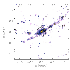
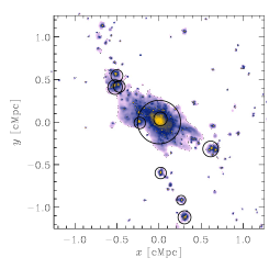
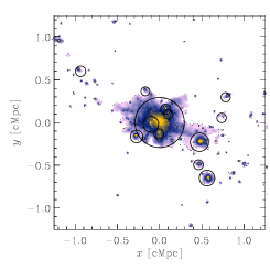
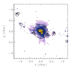
Halo stars    $T$=1 Gyr                            $T$=2 Gyr                            $T$=3 Gyr                            $T$=4 Gyr

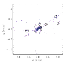
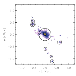
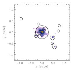
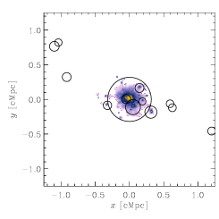
Figure 7: Spatial distribution of stars that ended up in the main galaxy at $z=0$, after $1$, $2$, $3$ and $4$ Gyr of evolution. The upper panels include the whole stellar population, while the lower panels are restricted to stars that ended up in the stellar halo component. The black circles show the position of the main progenitor and the most massive satellite galaxies at the varios times; their sizes are scaled with the corresponding masses. The colour scale represents the density of stellar mass in logarithmic scale, to allow a better visualization of the halo stars and their spatial location.

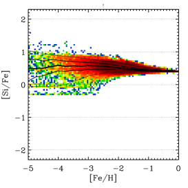
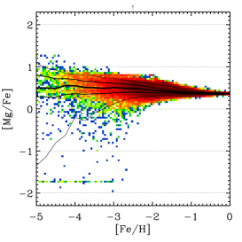
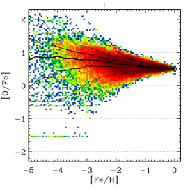
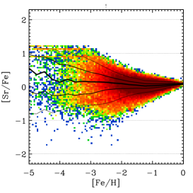
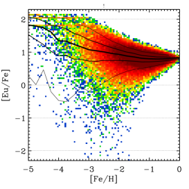
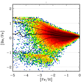
Figure 8: The various abundance ratios as a function of [Fe/H] for the halo stars in our simulation ME. The solid thick lines show the corresponding median values and the thin lines denote the $90$ $70$, $30$ and $10$ percentiles of the distributions. The colour scale is also shown.

In the cosmological context, galaxies grow via the continuous aggregation of matter and smaller substructures which can contribute distinct chemical patterns determined by the properties of the star formation activity within them and the characteristics of their accretion onto a larger system. In the simulation, we can trace back the formation of the $z=0$ system identifying, at each time, the main progenitor – i.e. the most massive structure at that time – and a series of smaller systems that later accreted onto the main progenitor.

Figure 7 shows a series of snapshots of the distribution of all stars that ended up in the main progenitor at $z=0$ (upper panels), and in the stellar halo component (lower panels). We focus on the early evolution, and show the distributions at 1, 2, 3 and 4 Gyr, characteristic of the formation and accretion of today’s halo stars (recall that, by definition, halo stars formed in the first 1Gyr of evolution, but they could have been accreted onto the main progenitor later on). The figures are centered at the mass center of the main progenitor at the different times, and the circles indicate the position and size of the different subhalos of the simulation, including the main progenitor. The upper panels of this figure reveal that, as expected within the cosmological context considered, the stellar component of the simulated galaxy has a contribution of material formed in systems other than the main progenitor. If we consider all stars that form the $z=0$ progenitor (i.e. all stellar components), the fraction of stellar mass that has been accreted is low.

However, the simulated stellar halo has significant contribution of ex-situ stars that formed outside the main progenitor, as can be seen from the lower panels of Figure 7. The ex-situ fraction of our simulated halo is $0.8$, i.e., only 20$\%$ of the stars in today’s halo formed in the main progenitor. This means that most halo stars formed in smaller, more metal-poor systems, with more episodic star formation activity, compared to the main progenitor. A high ex-situ fraction of the stellar halo is consistent with observations of the Milky Way stellar halo, although in our simulation many small satellites contributed to the stellar halo, while recent discoveries suggest that a large part of the Milky Way’s stellar halo could be the result of an early and massive accretion event (Helmi et al. 2018; Belokurov et al. 2019 - see review by Helmi 2020 and references therein).

It is worth noting that the ex-situ stars that end up in the stellar halo at $z=0$ locate preferentially in the outskirts of their systems before accretion, as evidenced from the lower panels of the figure. The reason for this behaviour is that stars in the outer regions are the less bound stars, likely to be lost during the merger. As a result, these stars stay in the halo component and are not able to reach the bulge region, unlike the central, most bound stars in the satellites. How this compares to the most recent observations of the Milky Way bulge will be addressed in a following paper.

As we discuss in the next subsections, the high contribution of accreted stars to the stellar halo leaves imprints in the $z=0$ chemical properties of this component, particularly in the case of neutron-capture elements.

4.2 Abundances ratios and scatter of halo stars

We discuss in this Section the predicted abundance ratios and scatter of stars in the simulated stellar halo at $z=0$ in our simulation ME. Fig. 8 shows the distributions of $\alpha-$ and neutron capture-elements, relative to Fe, as a function of the [Fe/H] abundance. The black thick lines indicate the median of the distributions, while the thin lines denote the $90$, $70$, $30$ and $10$ percentile levels. Similarly to our findings for the isolated galaxy simulations, the various elements have particular abundance levels and, more importantly, they exhibit distinct dispersions. In particular, the $\alpha$-elements show lower scatter compared to the neutron-capture elements, and this effect is more pronounced in the low-metallicity regime. The $\sigma$ values, estimated as half the difference between the values corresponding to the $70$ and $30$ percentiles of the distributions, as a function of [Fe/H], are shown in Fig. 9 for the various elements. Note that the scatter varies significantly with the [Fe/H] abundance, such that the higher the metallicity, the lower the scatter. The typical scatter for the $\alpha-$elements is $<\kern-11.99998pt\lower 4.73611pt\hbox{$\sim$}~{}0.35$ dex, while for the neutron capture elements the scatter levels are systematically and significantly higher, particularly for [Fe/H]$<\kern-11.99998pt\lower 4.73611pt\hbox{$\sim$}~{}-2.5$. Ba is the element with the highest $\sigma$ values, with Si having the lower dispersion levels.

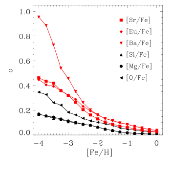
Figure 9: Estimation of the scatter $\sigma$ of the various abundance ratios of halo stars, as a function of [Fe/H], in our cosmological simulation ME. The $\sigma$ value has been calculated as half the difference between the abundance ratios corresponding to the $70$ and $30$ percentiles of the distributions.

Figure 10: Normalized distributions of stellar ages of halo stars, separated by ex-situ (solid lines) and in-situ (dashed lines) populations.

The different scatter levels are the result of the chemical yields and their dependence with the stellar mass and metallicity, which varies between the $\alpha-$ and neutron capture-elements, and also between elements of the same group. This is because the predictions of the simulation for the different elements and their scatter depend on how the yields for each element change with the stellar mass and metallicity. In particular, the Si yields are more tightly connected to iron and therefore the scatter is the smallest for the $\alpha-$elements. In the case of the neutron capture-elements, it is important to note that Eu is almost completely produced by r-processes, contrary to Ba and Sr which are also produced via s-processes, and therefore the different n-capture elements have different scatter levels.

It is worth noting that considering the cosmological evolution produces, as expected, more complex abundance ratio distributions compared to the results obtained with our idealized simulations of isolated galaxies. In particular, a small but non-negligible fraction of stars have [Ba/Fe]$<\kern-11.99998pt\lower 4.73611pt\hbox{$\sim$}~{}-1$, different from the overall distribution which has higher [Ba/Fe] values. We discuss the origin of this group in the next Sections.

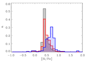
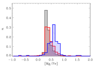
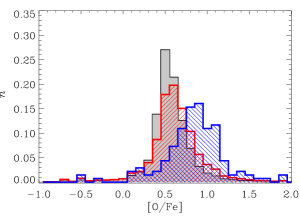
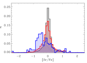
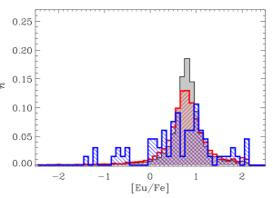
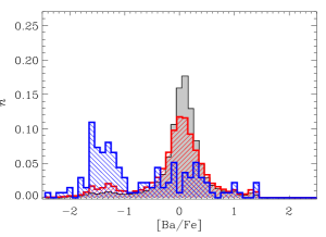
Figure 11: Normalized distribution functions of the various element ratios for our fiducidal halo sample, which assumes an age threshold for halo stars of $\tau=1$ Gyr (black line with grey shade). We also show results for the very old stars, formed until 100 Myr after the formation of the first star ($\tau=0.24$ Gyr, blue), and for an intermediate value of $\tau=0.5$ Gyr (red). Note that the various panels have different $x-$ranges in order to highlight the features of the distributions for different elements.

4.3 Fingerprints of formation history on abundances and scatter

As discussed above, the chemical properties of the stars encode information on the enrichment history; in the case of the halo stars the very old populations are particularly sensitive to the early stages of enrichment that follows the beginning of the star formation (SF) activity. In our cosmological simulation ME, the enrichment history is much more complex than the one obtained in the isolated case (Section 3), as stars that form the present-day stellar halo were formed in different systems, each of them with its own SF and enrichment properties. In particular, the onset of SF in the main progenitor and in the smaller satellites can occur at different times, and the SF rates can have different levels depending on the mass of the system. In our simulation, the very old stars of today’s halo were formed mainly ex-situ and, furthermore, the ex-situ stars have a higher fraction of very old stars compared to the in-situ component, as can be seen from Fig. 10 where we show the formation time distributions of the ex-situ and in-situ populations (normalized separately for clarity, as ex-situ stars are highly dominant).

The very old stars have in fact a significant impact on the element ratios, producing particular features that are not seen for the rest of the stellar halo population. Furthermore, such impact depends strongly on the chemical element considered and the characteristics of their yields and corresponding mass/metallicity dependencies. Fig. 11 shows the various abundance ratios for the halo stars (i.e. our fiducidal sample, assuming a formation time threshold of $\tau=1~{}$Gyr, black lines), as well as for the very old stars with $\tau=240$ Myr (i.e., 100 Myr after the formation of the first star, blue) and for an intermediate age threshold of $\tau=0.5~{}$Gyr (red). In the case of the $\alpha$-elements, restricting the sample to older populations produces a shift to higher abundances, because enrichment with these elements is faster compared to iron: even though both the $\alpha-$elements and iron are produced in SNII, the iron yields are comparatively lower for metal-poor stars. For $\tau=240$ Myr, the interstellar medium did not yet have time to enrich sufficiently so that the most massive stars produce significant amounts of $\alpha$-elements compared to iron.

In contrast, for the neutron-capture elements Sr and Ba we find that the very old stars have lower abundance ratios compared to the fiducidal halo sample, with larger scatter. For Eu, the abundances are similar, but the scatter is also larger when we consider the very old stars. In this case, stars formed from non/low contaminated gas produce both iron and the neutron-capture elements in the same progenitors, but as the interstellar medium is contaminated, enrichment with iron occurs faster compared to the neutron-capture elements. For this reason, once the very early stages of star formation have completed, the interstellar medium becomes more homogeneous, producing narrower abundance ratio distributions. In the case of the scatter, considering the very old stars produces wider distributions for all elements, because the interstellar medium is less homogeneous compared to later times.

The case of [Ba/Fe] is particularly important, as we have already seen that the [Ba/Fe] versus [Fe/H] distribution showed the presence of a stellar group with [Ba/Fe]$<-1$, different from the overall population. From Fig. 11 it is clear that it is the very old stars that contribute to this group, and these are also the stars that populate the lowermost [Sr/Fe] tail.

4.4 The [Sr/Ba] ratio

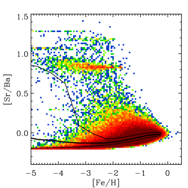
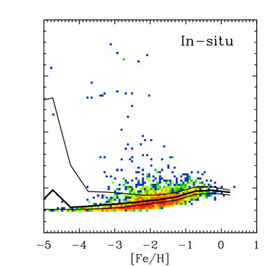
Figure 12: [Sr/Ba] abundance as a function of [Fe/H] for all halo stars (left-hand panel) and restricting the sample to the in-situ population (left-hand panel). The solid thick lines indicate the median of the distributions, and the thin lines show the corresponding $70$ and $30$ percentiles. The colour scale is also shown.

The [Sr/Ba] ratio is an important chemical ratio, as it is sensitive to the origin of the heavy elements. Observationally, not only the [Sr/Fe] and [Ba/Fe] abundances show a dispersion in our Galactic halo, but also their ratio [Sr/Ba] is not constant (François et al., 2007). These observations confirm the need for a second neutron-capture process which synthesised differently the light elements (such as Sr) and the heavy ones (as Ba), in addition to the r-process. Early contribution from fast rotating massive stars to s-process elements has been proposed (Pignatari et al., 2008; Chiappini et al., 2011; Frischknecht et al., 2012; Chiappini, 2013), as normal s-process enrichment by AGBs operates on long time-scales ($>300$ Myr, see Cescutti et al. 2006); moreover, at low metallicity, [Sr/Ba]$<0$ is expected from AGB nucleosynthesis (Cristallo et al. 2009, see also Frebel 2018).

These ideas were incorporated in stochastic inhomeogenous chemical evolution models which were able to predict a scatter in the [Sr/Ba] ratio (Cescutti et al., 2013; Cescutti & Chiappini, 2014). These models however, not being in the cosmological framework, do not take into account additional scatter caused by the addition of ex-situ stars resulting from mergers. These smaller galaxies would have their own star formation histories which, in principle, could add more scatter into the more simplified picture of the stochastic inhomogenous chemical evolution models. This is in fact what we see in our cosmological simulations.

The left-hand panel of Fig. 12 shows the [Sr/Ba] abundance ratio for halo stars, as a function of the [Fe/H] abundance. Halo stars have diverse [Sr/Ba] ratios, in the range $-0.2$ to $1.3$ dex; stars with [Fe/H]$\gtrsim-2$ have near solar abundances, but low metallicity stars appear both at sub-solar values and at [Sr/Ba]$\sim 0.8$, although at a lower rate.

It is worth noting that the simulation predicts a high scatter for [Sr/Ba], due to the combined pollution via r- and s-processes in fast rotating massive stars, our implementation of the differential enrichment of stars with different masses, and the cosmological evolution.

An important feature of this figure, which follows the characteristics of the [Ba/Fe] and [Sr/Fe] abundances seen above, is the stellar group with [Sr/Ba]$\sim 0.8$, different from the overall population. Such abundance ratios are only seen for the ex-situ population, and dissapear if we only consider the in-situ stars, as can be observed from the right-hand panel of Fig. 12. However, note that the key ingredient for forming the high [Sr/Ba] stars is the time-scale, because it is only the very old stars that produced such high ratios. This can be seen from Figure 13, where we show the [Sr/Ba] distributions for our fiducidal halo sample with $\tau=1$ Gyr (black), as well as for $\tau=0.5$ Gyr (red) and for the very old stars, with $\tau=0.24$ Gyr (blue). According to our simulation, the existence of the high [Sr/Ba] stars is a result of the enrichment time-scales for rotating massive stars compared to those assumed for the r-process, to the ages of accreted stars and to the slower enrichment occuring in the small systems that contribute to the formation of the stellar halo, compared to that of the main progenitor.

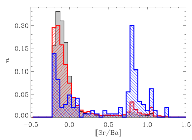
Figure 13: Normalized distribution functions of [Sr/Ba] in simulation ME, for our fiducidal halo sample, which assumes an age threshold for halo stars of $\tau=1$ Gyr (black line with grey shade). We also show results for the very old stars, formed until 100 Myr after the formation of the first star ($\tau=0.24$Gyr, red), and for an intermediate value of $\tau=0.5$ Gyr (red).

5 Discussion

The work presented here is a first implementation of the enrichment of various neutron-capture in cosmological simulations, and it might be relevant to compare, even at this early stage, to make a comparison with observational data. Note that a proper comparison with observations requires an extensive study on the probable observational biases and the selection of the most comparable stellar sample of the simulation, and this will be done in future work. In this Section, we make a broad comparison with observations, and we also compare our results with those from stochastic chemical evolution models which use the same chemical yields and stellar ages. Note that the scatter predicted in the simulation is more important than the exact levels obtained, as the abundance ratios can be easily changed by rescaling the yields, unlike the scatter which depends on the properties of their age/metallicity dependencies.

5.1 Simulations compared to observations

In this Section we compare our results for the abundance ratios and scatter of the different elements with the observations of Roederer et al. (2014) and Yong et al. (2013) (only carbon-normal stars), which provide data on the abundances of metal-poor stars in our Galaxy. Note that the comparison between simulations and observations is complex, and it needs to be taken with caution for various reasons. On one side, the observational samples are biased to low metallicity stars, and are complete only for the low metallicity range (approximately at [Fe/H] abundances lower than $-2.5$ or $-3$). Second, these observations are for stars in the solar vicinity, unlike the simulation data which include all stars in the simulated stellar halo. Also, the number of stars in both observational samples is relatively small and so there is no good statistics. Finally, it is worth noting that the two observational samples are not always compatible with each other, most notably in terms of the Si and Mg abundance ratios. Despite these difficulties, the two datasets are useful as they include the abundances of all or most of the chemical elements studied here.

Fig. 14 shows the predicted median values for the different elements, as a function of [Fe/H] (black lines), together with the $70/30$ and $90/10$ percentiles (dark and light shaded areas, respectively). The observations of Roederer et al. (2014) (solid black circles) and Yong et al. (2013) (enricled symbols) are also included, as well as the median and corresponding standard deviations in 0.5 dex wide bins (red triangles and blue diamonds, respectively), as to include at least 5 observational points per bin. We find that the predicted abundances for the $\alpha-$elements are consistent with the observations, particularly in the case of the Roederer et al. (2014) data set. On the other hand, the observations of Yong et al. (2013) for [Si/Fe] and [Mg/Fe] are in general below the predictions and also below the Roederer et al. (2014) observations. In terms of scatter, we find a good agreement for [Si/Fe] and [O/Fe], but the simulation predicts a higher scatter compared to the observations for the [Mg/Fe] ratio; the disagreement is more important for the low-metallicity regime. As explained above, the predictions for the scatter of the different $\alpha-$elements can vary due to the particular dependencies of the yields with the stellar mass and metallicity.

In the case of the neutron-capture elements, we find that the predicted ranges of [Sr/Fe] are consistent with the observational data but the [Ba/Fe] and [Eu/Fe] predicted values lie above the observations. Similarly, the scatter of [Sr/Fe] in the simulation is consistent with the data, but the scatter found for the other n-capture elements is higher in the simulation – this effect is more significant for lower metallicities. As explained above, Eu is almost completely produced by r-processes in contrast to the other n-capture elements, and so we expect different levels of scatter.

The discrepancies between the predicted and observed distributions for the neutron capture-elements can be interpreted as a signature that the real r-process contribution is more complex than what is assumed in this work. In fact, the rate of r-process production is fixed (from the narrow mass range of $8-10$M_⊙) and we do not consider any delay apart from the life-time of the considered stars. Moreover, our nucleosynthesis for the r-process component is determined in Cescutti et al. (2013) for Ba, and Eu is simply scaled based on the solar r-process residual that is the the same as the r-process ratio observed in r-process rich stars (Sneden et al., 2008). With these assumptions, our simulation overpredicts the [Eu/Fe] ratios compared to the data. It is worth mentioning that a similar outcome is observed in the Cescutti & Chiappini (2014) chemical evolution model which uses a similar approach. A possible solution would be to assume that the [Eu/Ba] ratio in the r-process is lower or not constant.

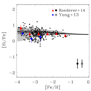
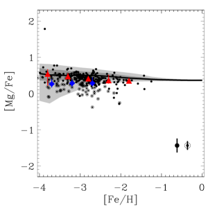
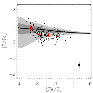
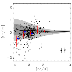
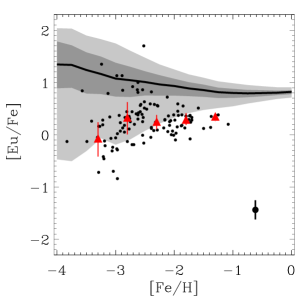
Figure 14: Median (black lines) and $90$, $70$, $30$ and $10$ percentiles (shaded regions) for the different element distributions in our halo stars in simulation ME. We also include the observations of Roederer et al. 2014 (solid black circles) and Yong et al. 2013 (encircled black symbols), as well as the median and corresponding standard deviations in 0.5 dex wide bins (red triangles and blue diamonds, respectively).

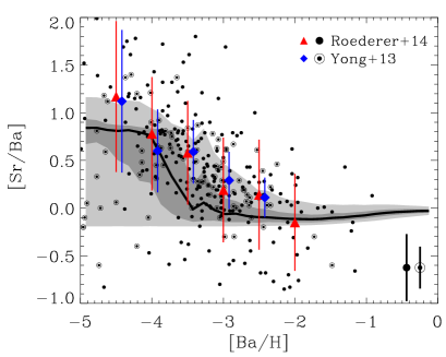
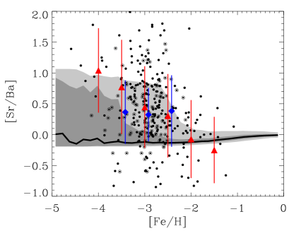
Figure 15: Median (black lines) and $90$, $70$, $30$ and $10$ percentiles (shaded regions) for the [Sr/Ba] ratio, as a function of [Ba/H] (left-pand panel) and [Fe/H] (right-hand panel) in our halo stars in simulation ME. We also include the observations of Roederer et al. 2014 (solid black circles) and Yong et al. 2013 (encircled black symbols), as well as the median and corresponding standard deviations in 0.5 dex wide bins (red triangles and blue diamonds, respectively).

Figure 15 compares the predicted distribution of [Sr/Ba] with observations. This figure shows [Sr/Ba] as a function of [Ba/H] (left-hand panel), which allows to better describe the two typical [Sr/Ba] ranges seen in Fig. 16 which overlap when we plot [Sr/Ba] as a function of [Fe/H] (right-hand panel). For the simulations, we show the median abundances of [Sr/Ba] for halo stars at $z=0$ (black lines), together with the 90, 70, 30 and 10 percentile levels (shaded areas). The observations of Roederer et al. (2014) (solid black circles) and Yong et al. (2013) (enricled black symbols) are also included as data points, as well as the median and corresponding standard deviations in 0.5 dex wide bins (red triangles and blue diamonds, respectively). The simulation and observations of [Sr/Ba] are consistent in general terms, and while the simulation median is systematically lower than the observational result, they both have a similar trend with the [Ba/H] abundance. Furthermore, the deviation around the mean for the simulation and the observations is similar, but in the simulation there are no stars with [Sr/Ba]$<-0.2$, a limit which is determined by the stellar yields adopted, particularly for the r-process. This is because for the early stages of chemical enrichment, the only relevant sources are the r-process events and the s-process products from rotating massive stars. The [Sr/Ba] ratio is fixed at $-0.2$ for the r-process events and, without rotating massive stars, we would obtain a fixed ratio for all stars in the simulation, as shown in Cescutti et al. (2013). The yields from massive stars at this metallicity can vary in the range $0<$[Sr/Ba]$<$2 according to Frischknecht et al. (2016b). Therefore, the final result is the mixing of these two sources which stay within these boundaries. Also, note that the absolute yields of r-process events are higher compared to those of rotating massive stars, therefore the former tend to dominate the final composition of stars in our model.

As we discussed above, the ex-situ stars formed very early on play a fundamental role in the scatter observed in the [Sr/Ba] ratio. Observationally, the contribution of satellites to the Milky Way stellar halo could be tested at least in two different ways. First, by studying the fractions of high and low [Sr/Ba] stars in present dSphs, and the possible dependence on galactic masses, e.g. whether the lightest galaxies are those with the highest [Sr/Ba] ratios. Previous works suggest that most classical and ultra faint dwarf galaxies have high [Sr/Ba] ratios (Venn et al. 2004; François et al. 2016) although Reticulum II is a small galaxy which got an early enrichment of r-process and shows a low [Sr/Ba] (Ji et al., 2016). Combining observations with simulations which provide a theoretical framework to understand how low and high [Sr/Ba] systems are formed and how they might contribute to the stellar halo of larger systems after accretion will likely help to better understand and interpret observational data. The second opportunity would be to check whether stars now in the Galactic halo with a high [Sr/Ba] show different characteristics from those with low or intermediate [Sr/Ba] ratio, which would point to their origin as debris of satellites merged to our halo (e.g. Helmi et al. 2018, see also Aguado et al. 2021; Limberg et al. 2021; Farouqi et al. 2022; Myeong et al. 2022). On this subject, Roederer et al. (2018) have found an indication that r-process rich stars could actually have belonged to small systems.

5.2 Simulations compared to inhomogeneous chemical evolution models

In this Section we compare the results of our simulation and the inhomogeneous chemical evolution models of Cescutti et al. (2013), focusing on the [Sr/Ba] abundance ratio. In Fig. 16 we show the [Sr/Ba] vs oxygen abundance distributions obtained with the Cescutti et al. (2013) model (left-hand panel) and with the cosmological simulations, for ex-situ (middle-hand panel) and in-situ (right-hand panel) halo stars separately. The simulation, particularly in the case of the ex-situ stars which are the dominant component of the stellar halo, predicts a broader range of oxygen abundances. At the metal-rich end, the stochastic models do not extend to very high oxygen abundances because the present-day metallicity distribution of the halo at the solar vicinity is used as a constraint. However, it is now known that large fraction of the stars between [Fe/H] = $-$1 and below are actually part of debris of galaxies accreted onto the Milky Way in the past (Helmi 2020 and references therein), and therefore are an ex-situ population, which is not included in the model. On the other hand, the low-metallicity tail in the Cescutti et al. (2013) model is affected by the low dilution of the contribution of a single SNII by the ISM, which is a free parameter. Given that the chemical evolution models are a much more simplified approach compared to the simulations, it is encouraging that results for the [Sr/Ba] abundances and scatter are similar, particularly in the case of the ex-situ stars.

Note that, consistently with the results obtained with the cosmological simulation (Section 4.4), in the stochastic model the high-[Sr/Ba] population is very old, formed before the r-process events start to enrich the ISM. The reason is that in the stochastic volume the mixing is instantaneous and the typically abundant r-process enrichment erases the chemical signature of the rotating massive stars pollution. We expect this outcome to be correct even if we consider a different r-process event, as it is the case for the stochastic approach (as illustrated in Cescutti & Chiappini 2014 for magneto-rotational driven SNe and in Cescutti et al. 2015 for neutron star mergers), although the exact definition of the age range expected for these stars can vary depending on the nucleosynthesis assumptions. This stresses the importance to obtain a high-resolution in age estimations in the very early phases of the galaxy assembly. The first steps in this direction were recently shown by Montalbán et al. (2021).

Cescutti et al. (2013)                                Ex-situ                                         In-situ

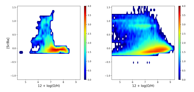
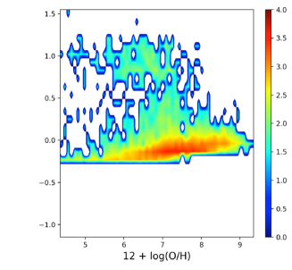
Figure 16: Distribution of [Sr/Ba] as a function of oxygen abundance for the halo stars in the Cescutti et al. 2013 model (left-hand panel), and the ex-situ (middle-hand panel) and in-situ (right-hand panel) components of the stellar halo in our cosmological simulation.

6 Conclusions

In this paper we present a novel implementation of chemical enrichment in hydrodynamical, cosmological simulations, which considers the production of $\alpha-$ and neutron-capture elements, and their distribution into the interstellar medium during SNII explosions. The novel aspect of our work is twofold: first, we use chemical yields which consider the impact of the rotation of massive stars at low metallicity (Cescutti & Chiappini, 2014; Cescutti et al., 2015) and, second, we consider the differential enrichment due to the different life-times of stars of different mass within the massive star range. In other words, we do not use IMF weighted yields for core collapse SNe. This means that the star particles of the simulations, which represent a mix of individual stars with given masses, explode in several episodes rather than at a single time, as usually done in this type of numerical studies. This might produce small variations in the overall chemical properties of galaxies; however, it has a critical role for the oldest/most metal-poor stars which are severely affected by the early enrichment stages, a point which we demonstrated here.

The main aim of the work was to investigate whether our model can reproduce the different scatter levels for the abundance ratios of the $\alpha-$ and neutron-capture elements, as suggested by observations of old stars in our Galaxy. We focused on the abundance ratios and scatter of the neutron-capture elements Ba, Eu and Sr, and the $\alpha-$elements O, Si and Mg, relative to the Fe abundance, and compared the predictions of simulations that assumed either one or multiple explosions per star particle – i.e. the “single explosion” (SE) and “multiple explosions” (ME) models. All simulations of this work assumed, for the ME model, a number of 5 explosions per SNII event. With this choice, we can properly describe the enrichment of the ISM avoiding large numerical overcosts.

Our implementation is grafted onto the gadget3 code (Springel et al., 2008) with the sub-grid modules of Scannapieco et al. (2005, 2006) for cooling, star formation, chemical enrichment and feedback from supernova (type II and Ia) explosions. As the current work focuses on the chemical abundances of the old stellar population, which are mainly determined by the products of SNII explosions, we have switched off the module for SNIa, as well as the Poulhazan et al. 2018 extensions for AGB stars, in all simulations presented here.

In order to validate and test our implementation, we run a number of idealized simulations of isolated galaxies, as well as the cosmological formation of a Milky Way-mass galaxy, and compared the chemical properties of the resulting systems for the SE and ME models. We found that the chemical abundance ratios obtained for all chemical elements are different for the SE and ME models: while in the former the abundance ratios are restricted to a narrow range given by the yields tables, the latter are able to produce much more diverse abundance ratios and higher scatter levels, in better agreement with observational results. The ME models produce a faster enrichment of the interstellar medium, because the first explosion event associated to star particles occurs earlier compared to the SE models, which affects the cooling, star formation and feedback levels at the very early times.

After passing the various numerical tests performed to our implementation, we focused on the chemical properties of the stellar halo formed in our cosmological simulation ME. Our main findings can be summarized as follows:

• The scatter found for the abundance ratios of neutron-capture elements (relative to iron) of the halo stars is larger compared to that of $\alpha$-elements. We find that the $\alpha$-elements have a typical scatter of the order of $<\kern-11.99998pt\lower 4.73611pt\hbox{$\sim$}~{}0.35$ dex (even at low metallicity), while for all neutron-capture elements studied here the scatter levels are systematically higher, with values $\gtrsim 0.3$ and up to $1$ dex for [Fe/H]$<-2.5$. For both types of elements, the scatter increases for decreasing metallicity, although this trend is much more pronounced for the neutron-capture elements.

• The scatter levels of the various elements are affected by the cosmological evolution: in our simulation, most stars that form the present-day stellar halo ($\sim 80\%$) formed ex-situ and later accreted onto the main progenitor. The oldest stars formed in the satellites present particular features in the abundance ratios, most notably in the case of n-capture elements, that are fingerprints of the ISM levels of enrichment at very early times.

• Our model also predicts a high scatter for the [Sr/Ba] ratio in halo stars, and a non-negligible fraction of stars with [Sr/Ba]$\sim 0.8$. The high [Sr/Ba] ratios are driven by the pollution via the fast-rotating stars at very early times.

In summary, the main reasons for obtaining different levels of scatter for the neutron-capture and $\alpha-$elements are the dependence of the stellar yields on the properties of the massive stars and the description of the differential enrichment during the early phases. The early enrichment of the ISM leaves an imprint in the abundances of the very old stars, in terms of the abundances and scatter of particular elements. This opens the possibility to reconstruct the enrichment level of galaxies at early epochs from observational data of the old stars, information that is otherwise inaccessible.

The success of our implementation in reproducing the scatter levels of the different elements allows to study, in a much more realistic manner than possible before, the chemical properties of all old stellar components in galaxies, most notably the bulge, which is the subject of the next paper of this series. In combination with the effects of SNIa and AGB stars, these models have the potential to provide detailed chemical abundances for all components in galaxies, which can be used to put additional constrains on the sub-grid physics describing star formation and feedback, and that are necessary to provide more predictive power to simulations in the $\Lambda$CDM cosmology.

Data Availability

The data underlying this article will be shared on reasonable request to the corresponding author.

Appendix A Additional tests of the code

A.1 The effects of resolution

In this Section we test the effects of resolution on our results, by comparing simulations using the idealized initial conditions of Section 3 and varying the number of particles, $N$ (note that $N$ refers here to the number of particles in one dimension, i.e. the total number of particles of the simulation is $N_{\rm tot}\sim N^{3}$). In particular, we compare the runs with $N=64$ of Section 3 (i.e. SE64 and ME64) with identical tests using $N=32$ and $N=128$ Following our naming convention used in this work, we refer to the simulations as SE/ME to refer to the single/multiple events per SN explosion, followed by the number $N$ denoting the number of particles. The mass resolution of the simulations with $N=32,64$ and $128$ is, respectively, $600$, $70$ and $9\times 10^{4}$ M_⊙ for the gas particles and $500$, $60$ and $8\times 10^{5}$ M_⊙ for dark matter particles, and we have used the same gravitational softenings in all runs.

The left- and middle-hand panels of Fig. 17 compare the SFR and cumulative stellar mass as a function of time for our various tests. The runs with $N=64$ and $128$ show very good convergence, particularly at the early times when the star formation activity is at its maximum. In contrast, the lowest resolution runs show somewhat stronger differences. In the SE case, the star formation rate at late times is significantly lower than their counterparts in the runs with higher resolution, although this is not significant in terms of the total stellar mass formed. For ME32, the differences are more important, and appear right at the peak of star formation, producing a noticeable difference, with respect to ME64 and ME128, in the evolution of the stellar mass formed. We note that simulations using multiple events per SN explosion are expected to induce more important differences because the changes in chemical abundance that occur right after the first SN explosions translate into changes in the cooling and the subsequent star formation activity. The faster enrichment in the ME simulations can be observed from the right-hand panel of Fig. 17 where we show the evolution of the total stellar metallicity of our tests with different resolution. After 1 Gyr of evolution, and regardless of resolution, the ME runs have have significantly higher metallicities compared to the SE tests.

We have also studied the effects of resolution on the predicted element ratios after 1 Gyr of evolution. As an example, we show in Fig. 18 the results of the ME32, ME64 and ME128 runs, for [O/Fe] and [Ba/Fe]. We find very similar results in all cases, indicating that resolution effects, particularly for $N\geq 64$, are unimportant. Note the very good agreement for the mean/dispersion values, as clearly seen from the right-hand panel of this figure, despite the expected differences in terms of higher resolutions being able to better sample stars at the extremes of the distributions. We conclude that our models are robust against resolution provided $64^{3}$ or more particles are used.

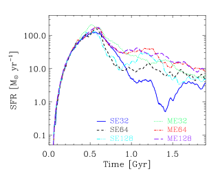
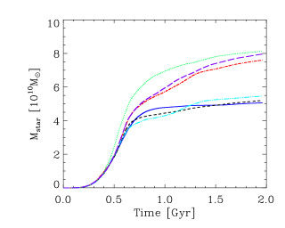
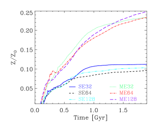
Figure 17: Star formation rates and integrated stellar mass and metallicity as a function of time for our simulations with single/multiple explosion times per SN event and various resolutions.

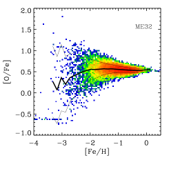
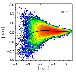
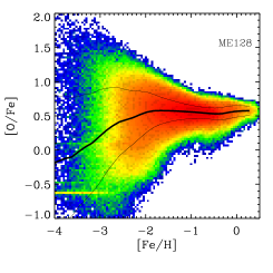
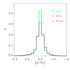
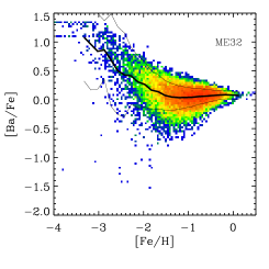
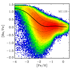
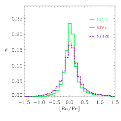
Figure 18: The distribution of [O/Fe] and [Ba/Fe] versus [Fe/H] for our simulations assuming multiple events per SN explosion and different number of particles, after 1 Gyr of evolution. The colour scale is normalized to the total number of star particles in each simulation, and we also show the corresponding median (thick lines) and $\pm\sigma$ contours (thin lines). The right-hand panel shows a quantitative comparison of the three distributions.

A.2 Dependence on number of SPH neighbours

We discuss in this Section the effects of varying the number of SPH neighbours, which determine the spatial extent over which metals are distributed after SN explosion events. This could have an effect on the predicted distributions of chemical abundances through the effects on the mixing of elements in the interstellar medium. In order to investigate this we have run additional tests, both for the SE and ME models, where we increased the number of neighbours from the fiducidal value of $N_{\rm ngb}=40$ (used in the SE64 and ME64 simulations of Section 3) to $64/128$.

Fig. 19 compares the SFR and the evolution of the stellar mass and metallicity for these tests. We find very good convergence of the tests until the peak of the star formation rate, when differences become more significant. In particular, an increase in $N_{\rm ngb}$ translates into an enhancement of star formation activity, which is produced because the chemical elements that are distributed after SN explosions spread over comparatively larger regions. Note that this effect is most clear right after the SF peak, as later on the effects of varying the number of SPH neighbours becomes non trivial: on one hand, the polluted regions are larger enhancing the cooling efficiency and star formation activity, while, on the other, higher SFRs produce larger amounts of feedback that reduce subsequent star formation levels.

Following the behaviour of the SFRs, the total stellar mass formed is in general larger for the simulations with larger $N_{\rm ngb}$, with more significant differences in the case of the SE runs. A similar behaviour is detected in the case of the stellar metallicities, where differences are more important for the SE runs and not significant for the ME tests. Variations in the stellar metallicity follow the variations in the stellar masses, such that runs with larger $N_{\rm ngb}$ are systematically more enriched.

Finally, we show in Fig. 20 the results of runs with different number of neighbours, for [O/Fe] and [Ba/Fe] after 1 Gyr of evolution, and their comparison. We find very similar results for both element ratios, indicating that our results are robust against changes in $N_{\rm ngb}$. Note the excellent agreement of the mean values and also of the scatter, evidenced in the right-hand panel of this figure. We conclude that the results of our model are robust against changes in the number of SPH neighbours used in the simulations.

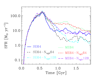
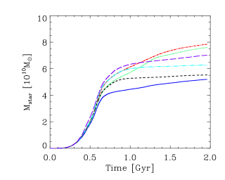
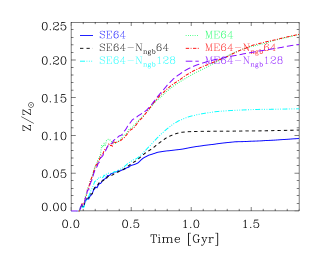
Figure 19: Star formation rates and integrated stellar mass and stellar metallicity as a function of time for our simulations with single/multiple explosion times per SN event and various choices for the number of SPH neighbours.

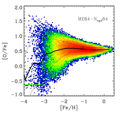
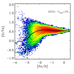
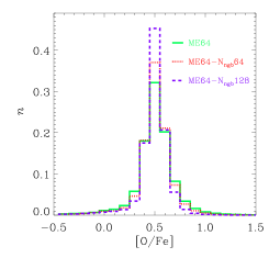
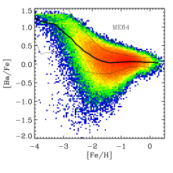
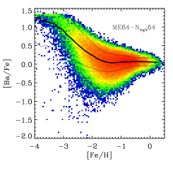
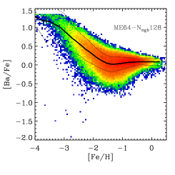
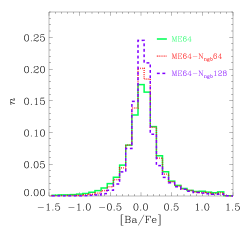
Figure 20: The distribution of [O/Fe] and [Ba/Fe] versus [Fe/H] for our simulations assuming multiple events per SN explosion and different number of SPH neighbours, after 1 Gyr of evolution. The colour scale is normalized to the total number of star particles in each simulation, and we also show the corresponding median (thick lines) and $\pm\sigma$ contours (thin lines). The right-hand panel shows a quantitative comparison of the three distributions.

Appendix B Cosmological simulations

In this Appendix we show that the effects of differential enrichment on the chemical properties of the old stars, discussed in Section 3, are reproduced in cosmological simulations. For this, we compare the results of cosmological simulations SE and ME (see Table 1), which assume a single or multiple explosions per SNII, respectively. As explained in Section 4, these correspond to cosmological simulations of a Milky Way-mass galaxy. In order to show that differential enrichment affects the properties of old stars, we focus here on stars formed during the first Gyr of evolution (which also allows comparison with our idealized simulations), even though the cosmological simulations have been run up to $z=0$.

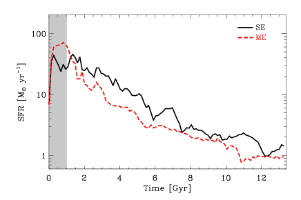
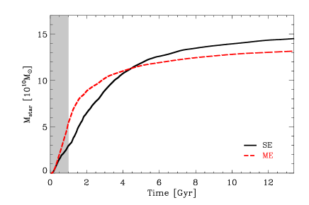
Figure 21: Evolution of the star formation rate (upper panel) and integrated stellar mass (lower panel) for our cosmological simulations SE and ME, which assume single and multiple events per SN explosion, respectively. The shaded area highlights the first 1Gyr of evolution, where we focus our study.

Fig. 21 shows the SFRs and evolution of the stellar mass in simulations SE and ME. Similarly to our findings of the idealized simulations, ME has a higher SFR compared to ME during the first Gyr of evolution, due to the faster enrichment of the ISM when multiple events per SNII are assumed and the enhanced cooling rates. Later on, however, the behaviour of the SFRs inverts, as the amount of feedback in ME is larger than in SE, producing a stronger reduction of the star formation activity after the first starburst. As a result, at the end of the simulation the galaxy formed in ME has lower stellar mass.

In Fig. 22 we compare the distributions of the various element ratios in SE and ME for stars formed during the 1 Gyr of evolution. We show results for all these stars and, because differences are expected to be more important for the very metal-poor stars, we show the same distributions restricting the sample according to the [Fe/H] abundance. The differences between SE and ME are dramatic, and confirm that the proper treatment of the early chemical enrichment significantly affects the scatter of the various element ratios. ME predicts much broader element ratio distributions compared to SE, and this effect is sronger as we move to more metal-poor populations. These results are consistent with our findings using the idealized simulations. It is worth noting that SE is unable to produce broad element ratio distributions, even though the cosmological setting is taken into account. This means that it is the differential enrichment what induces the scatter in the distributions, despite the fact that the cosmological evolution could add even more scatter. In particular, in the case of the stellar halo we expect a high contribution of ex-situ stars adding to this scatter (see Section LABEL:sec:high_srba.

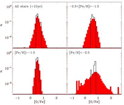
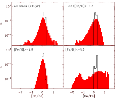
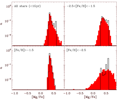
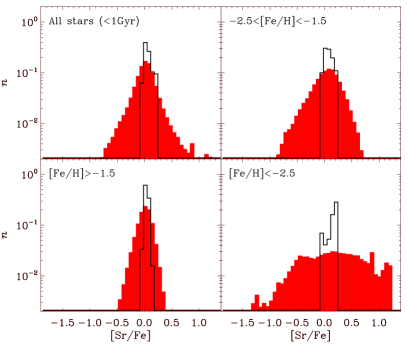
Figure 22: Distribution functions of various stellar abundance ratios, for our cosmological simulations SE (solid lines) and ME (shaded areas), at $z=0$, considering only the old stars (formed during the first Gyr of evolution). The different panels show distributions for four ranges in [Fe/H].

References

- Aguado et al. (2021) Aguado D. S., et al., 2021, ApJ, 908, L8
- Argast et al. (2004) Argast D., Samland M., Thielemann F. K., Qian Y. Z., 2004, A&A, 416, 997
- Belokurov et al. (2018) Belokurov V., Deason A. J., Koposov S. E., Catelan M., Erkal D., Drake A. J., Evans N. W., 2018, MNRAS, 477, 1472
- Belokurov et al. (2019) Belokurov V., Deason A. J., Erkal D., Koposov S. E., Carballo-Bello J. A., Smith M. C., Jethwa P., Navarrete C., 2019, MNRAS, 488, L47
- Brauer et al. (2020) Brauer K., Ji A. P., Drout M. R., Frebel A., 2020, arXiv e-prints, p. arXiv:2010.15837
- Busso et al. (1999) Busso M., Gallino R., Wasserburg G. J., 1999, ARA&A, 37, 239
- Caughlan & Fowler (1988) Caughlan G. R., Fowler W. A., 1988, Atomic Data and Nuclear Data Tables, 40, 283
- Cayrel et al. (2004) Cayrel R., et al., 2004, A&A, 416, 1117
- Cescutti (2008) Cescutti G., 2008, A&A, 481, 691
- Cescutti & Chiappini (2010) Cescutti G., Chiappini C., 2010, A&A, 515, A102
- Cescutti & Chiappini (2014) Cescutti G., Chiappini C., 2014, A&A, 565, A51
- Cescutti et al. (2006) Cescutti G., François P., Matteucci F., Cayrel R., Spite M., 2006, A&A, 448, 557
- Cescutti et al. (2013) Cescutti G., Chiappini C., Hirschi R., Meynet G., Frischknecht U., 2013, A&A, 553, A51
- Cescutti et al. (2015) Cescutti G., Romano D., Matteucci F., Chiappini C., Hirschi R., 2015, A&A, 577, A139
- Chiappini (2013) Chiappini C., 2013, Astronomische Nachrichten, 334, 595
- Chiappini et al. (2006) Chiappini C., Hirschi R., Meynet G., Ekström S., Maeder A., Matteucci F., 2006, A&A, 449, L27
- Chiappini et al. (2008) Chiappini C., Ekström S., Meynet G., Hirschi R., Maeder A., Charbonnel C., 2008, A&A, 479, L9
- Chiappini et al. (2011) Chiappini C., Frischknecht U., Meynet G., Hirschi R., Barbuy B., Pignatari M., Decressin T., Maeder A., 2011, Nature, 472, 454
- Choplin et al. (2018) Choplin A., Hirschi R., Meynet G., Ekström S., Chiappini C., Laird A., 2018, A&A, 618, A133
- Cowan et al. (2021) Cowan J. J., Sneden C., Lawler J. E., Aprahamian A., Wiescher M., Langanke K., Martínez-Pinedo G., Thielemann F.-K., 2021, Reviews of Modern Physics, 93, 015002
- Cristallo et al. (2009) Cristallo S., Straniero O., Gallino R., Piersanti L., Domínguez I., Lederer M. T., 2009, ApJ, 696, 797
- Farouqi et al. (2022) Farouqi K., Thielemann F. K., Rosswog S., Kratz K. L., 2022, A&A, 663, A70
- François et al. (2004) François P., Matteucci F., Cayrel R., Spite M., Spite F., Chiappini C., 2004, A&A, 421, 613
- François et al. (2007) François P., et al., 2007, A&A, 476, 935
- François et al. (2016) François P., Monaco L., Bonifacio P., Moni Bidin C., Geisler D., Sbordone L., 2016, A&A, 588, A7
- Frebel (2018) Frebel A., 2018, Annual Review of Nuclear and Particle Science, 68, 237
- Frischknecht et al. (2012) Frischknecht U., Hirschi R., Thielemann F. K., 2012, A&A, 538, L2
- Frischknecht et al. (2016a) Frischknecht U., et al., 2016a, MNRAS, 456, 1803
- Frischknecht et al. (2016b) Frischknecht U., et al., 2016b, MNRAS, 456, 1803
- Gaia Collaboration, Brown et al. (2018) Gaia Collaboration, Brown A. G. A., et al., 2018, A&A, 616, A1
- Gaia Collaboration, Brown et al. (2021) Gaia Collaboration, Brown A. G. A., et al., 2021, A&A, 650, C3
- Grevesse et al. (2010) Grevesse N., Asplund M., Sauval A. J., Scott P., 2010, Ap&SS, 328, 179
- Gudin et al. (2021) Gudin D., et al., 2021, ApJ, 908, 79
- Guidi et al. (2016) Guidi G., Scannapieco C., Walcher J., Gallazzi A., 2016, MNRAS, 462, 2046
- Gull et al. (2021) Gull M., Frebel A., Hinojosa K., Roederer I. U., Ji A. P., Brauer K., 2021, ApJ, 912, 52
- Haynes & Kobayashi (2019) Haynes C. J., Kobayashi C., 2019, MNRAS, 483, 5123
- Helmi (2020) Helmi A., 2020, ARA&A, 58, 205
- Helmi et al. (2018) Helmi A., Babusiaux C., Koppelman H. H., Massari D., Veljanoski J., Brown A. G. A., 2018, Nature, 563, 85
- Hirschi (2007) Hirschi R., 2007, A&A, 461, 571
- Honda et al. (2004) Honda S., Aoki W., Kajino T., Ando H., Beers T. C., Izumiura H., Sadakane K., Takada-Hidai M., 2004, ApJ, 607, 474
- Ji et al. (2016) Ji A. P., Frebel A., Simon J. D., Geha M., 2016, ApJ, 817, 41
- Kennicutt (1998) Kennicutt Jr. R. C., 1998, ARA&A, 36, 189
- Koppelman et al. (2019) Koppelman H. H., Helmi A., Massari D., Roelenga S., Bastian U., 2019, A&A, 625, A5
- Limberg et al. (2021) Limberg G., et al., 2021, ApJ, 913, L28
- Limongi & Chieffi (2018) Limongi M., Chieffi A., 2018, ApJS, 237, 13
- Maeder & Meynet (1989) Maeder A., Meynet G., 1989, A&A, 210, 155
- Majewski et al. (2017) Majewski S. R., et al., 2017, AJ, 154, 94
- McWilliam (1998) McWilliam A., 1998, AJ, 115, 1640
- Meynet & Maeder (2002) Meynet G., Maeder A., 2002, A&A, 390, 561
- Miglio et al. (2021) Miglio A., et al., 2021, A&A, 645, A85
- Montalbán et al. (2021) Montalbán J., et al., 2021, Nature Astronomy,
- Montes et al. (2007) Montes F., et al., 2007, ApJ, 671, 1685
- Myeong et al. (2019) Myeong G. C., Vasiliev E., Iorio G., Evans N. W., Belokurov V., 2019, MNRAS, 488, 1235
- Myeong et al. (2022) Myeong G. C., Belokurov V., Aguado D. S., Evans N. W., Caldwell N., Bradley J., 2022, arXiv e-prints, p. arXiv:2206.07744
- Naidu et al. (2020) Naidu R. P., Conroy C., Bonaca A., Johnson B. D., Ting Y.-S., Caldwell N., Zaritsky D., Cargile P. A., 2020, ApJ, 901, 48
- Naiman et al. (2018) Naiman J. P., et al., 2018, MNRAS, 477, 1206
- Navarro & White (1993) Navarro J. F., White S. D. M., 1993, MNRAS, 265, 271
- Nuza et al. (2014) Nuza S. E., Parisi F., Scannapieco C., Richter P., Gottlöber S., Steinmetz M., 2014, MNRAS, 441, 2593
- Pignatari et al. (2008) Pignatari M., Gallino R., Meynet G., Hirschi R., Herwig F., Wiescher M., 2008, ApJ, 687, L95
- Poulhazan et al. (2018) Poulhazan P.-A., Scannapieco C., Creasey P., 2018, MNRAS, 480, 4817
- Prantzos et al. (2018) Prantzos N., Abia C., Limongi M., Chieffi A., Cristallo S., 2018, MNRAS, 476, 3432
- Qian & Wasserburg (2000) Qian Y. Z., Wasserburg G. J., 2000, Phys. Rep., 333, 77
- Re Fiorentin et al. (2021) Re Fiorentin P., Spagna A., Lattanzi M. G., Cignoni M., 2021, ApJ, 907, L16
- Roederer et al. (2014) Roederer I. U., Preston G. W., Thompson I. B., Shectman S. A., Sneden C., Burley G. S., Kelson D. D., 2014, AJ, 147, 136
- Roederer et al. (2018) Roederer I. U., Hattori K., Valluri M., 2018, AJ, 156, 179
- Ryan et al. (1996) Ryan S. G., Norris J. E., Beers T. C., 1996, ApJ, 471, 254
- Sawala et al. (2010) Sawala T., Scannapieco C., Maio U., White S., 2010, MNRAS, 402, 1599
- Sawala et al. (2011) Sawala T., Guo Q., Scannapieco C., Jenkins A., White S., 2011, MNRAS, 413, 659
- Sawala et al. (2012) Sawala T., Scannapieco C., White S., 2012, MNRAS, 420, 1714
- Scannapieco et al. (2005) Scannapieco C., Tissera P. B., White S. D. M., Springel V., 2005, MNRAS, 364, 552
- Scannapieco et al. (2006) Scannapieco C., Tissera P. B., White S. D. M., Springel V., 2006, MNRAS, 371, 1125
- Scannapieco et al. (2008) Scannapieco C., Tissera P. B., White S. D. M., Springel V., 2008, MNRAS, 389, 1137
- Scannapieco et al. (2009) Scannapieco C., White S. D. M., Springel V., Tissera P. B., 2009, MNRAS, 396, 696 (S09)
- Scannapieco et al. (2010) Scannapieco C., Gadotti D. A., Jonsson P., White S. D. M., 2010, MNRAS, 407, L41
- Scannapieco et al. (2011) Scannapieco C., White S. D. M., Springel V., Tissera P. B., 2011, MNRAS, 417, 154
- Scannapieco et al. (2012) Scannapieco C., et al., 2012, MNRAS, 423, 1726
- Shen et al. (2015) Shen S., Cooke R. J., Ramirez-Ruiz E., Madau P., Mayer L., Guedes J., 2015, ApJ, 807, 115
- Sneden et al. (2008) Sneden C., Cowan J. J., Gallino R., 2008, ARA&A, 46, 241
- Springel & Hernquist (2003) Springel V., Hernquist L., 2003, MNRAS, 339, 289
- Springel et al. (2008) Springel V., et al., 2008, MNRAS, 391, 1685
- Sutherland & Dopita (1993) Sutherland R. S., Dopita M. A., 1993, ApJS, 88, 253
- Tissera et al. (2013) Tissera P. B., Scannapieco C., Beers T. C., Carollo D., 2013, MNRAS, 432, 3391
- Tissera et al. (2014) Tissera P. B., Beers T. C., Carollo D., Scannapieco C., 2014, MNRAS, 439, 3128
- Travaglio et al. (2004) Travaglio C., Gallino R., Arnone E., Cowan J., Jordan F., Sneden C., 2004, ApJ, 601, 864
- Valentini et al. (2019) Valentini M., et al., 2019, A&A, 627, A173
- Venn et al. (2004) Venn K. A., Irwin M., Shetrone M. D., Tout C. A., Hill V., Tolstoy E., 2004, AJ, 128, 1177
- Wanajo et al. (2001) Wanajo S., Kajino T., Mathews G. J., Otsuki K., 2001, ApJ, 554, 578
- Wehmeyer et al. (2015) Wehmeyer B., Pignatari M., Thielemann F. K., 2015, MNRAS, 452, 1970
- Wehmeyer et al. (2019) Wehmeyer B., Fröhlich C., Côté B., Pignatari M., Thielemann F. K., 2019, MNRAS, 487, 1745
- Woosley & Weaver (1995) Woosley S. E., Weaver T. A., 1995, ApJS, 101, 181
- Yong et al. (2013) Yong D., et al., 2013, ApJ, 762, 26
- van de Voort et al. (2015) van de Voort F., Quataert E., Hopkins P. F., Kereš D., Faucher-Giguère C.-A., 2015, MNRAS, 447, 140
- van de Voort et al. (2020) van de Voort F., Pakmor R., Grand R. J. J., Springel V., Gómez F. A., Marinacci F., 2020, MNRAS, 494, 4867