Cornering the Two Higgs Doublet Model Type II

Abstract

We perform a comprehensive study of the allowed parameter space of the Two Higgs Doublet Model of Type II (2HDM-II). Using the theoretical framework flavio we combine the most recent flavour, collider and electroweak precision observables with theoretical constraints to obtain bounds on the mass spectrum of the theory. In particular we find that the 2HDM-II fits the data slightly better than the Standard Model (SM) with best fit values of the heavy Higgs masses around 2 TeV and a value of $\tan\beta\approx 4$. Moreover, we conclude that the wrong-sign limit is disfavoured by Higgs signal strengths and excluded by the global fit by more than five standard deviations and potential deviations from the alignment limit can only be tiny. Finally we test the consequences of our study on electroweak baryogenesis via the program package BSMPT and we find that the allowed parameter space strongly discourages a strong first order phase transition within the 2HDM-II.

SI-HEP-2021-20, SFB-257-P3H-21-049

1 Introduction

Two Higgs Doublet Models (2HDM) Lee:1973iz (see Ref. Gunion:1989we for a textbook and Ref. Branco:2011iw for a more recent review) are very well-studied extensions of the Standard Model (SM) and probably one of the simplest possibilities for beyond the SM (BSM) physics. Besides the SM particles, four new scalars arise in the 2HDM: two charged ones ($H^{+}$ and $H^{-}$), a pseudoscalar ($A^{0}$, CP-odd) and a scalar ($H^{0}$, CP-even; when denoting the SM Higgs with $h^{0}$). Such an extension might solve some of the conceptual problems that arise within the SM, see e.g. Ref. Trodden:1998qg . In particular, 2HDMs could provide the missing amount of CP violation to explain the matter-antimatter asymmetry in the Universe and they could also lead to a first order phase transition in the early Universe, as required by the Sakharov criteria Sakharov:1967dj . 2HDMs further appear as subsets of more elaborate BSM models, such as the minimal supersymmetric SM (MSSM). Depending on the structure of the Yukawa couplings one distinguishes different types of 2HDMs – in this work we will consider the 2HDM-II.

Since we have no direct experimental evidence so far for an extended Higgs sector, we investigate indirect constraints on the 2HDM-II by comparing the most recent measurements with high precision calculations. We perform a comprehensive study of more than 250 observables, where the new Higgs particles could appear as virtual corrections and modify the SM prediction. Our study extends previous works like Refs. Deschamps:2009rh ; Chowdhury:2017aav . In 2009, Ref. Deschamps:2009rh studied bounds from quark flavour observables on the 2HDM-II within the framework of CKMfitter. In particular, it was found that the 2HDM does not perform better in the fit than the SM and that the new charged scalar has to be heavier than 316 GeV. We will considerably extend this analysis by using updated measurements, theory predictions and by including additional flavour observables. In 2017, the authors of Ref. Chowdhury:2017aav used HEPfit to constrain the 2HDM-II with Higgs data, electroweak precision observables and some flavour observables (the radiative decay $b\to s\gamma$ and the mass difference of neutral $B$ mesons $\Delta m_{q}$), as well as theoretical constraints like perturbativity. The main findings are lower mass bounds such as $m_{H^{+}}>740$ GeV and a lower limit on the mass splittings of the heavy Higgses of the order of 100 GeV. Higgs signal strengths allow only small deviations from the alignment limit, $|\beta-\alpha-\pi/2|<0.055$ - this bound is further reduced to $|\beta-\alpha-\pi/2|<0.02$ within the overall fit (driven by theory constraints). Finally, the authors of Ref. Chowdhury:2017aav found that the parameter $\tan\beta$ lies in the preferred range $[0.93;5.0]$. We will extend this analysis by updating experimental values and considering a large number of flavour observables. Moreover we confirm the observation made in Ref. Chowdhury:2017aav , that the wrong-sign limit is excluded by data.

Throughout this work, we use the Python program package flavio Straub:2018kue for flavour physics for our predictions of observables in the 2HDM-II. New physics models are not explicitly included in flavio. Instead, they impact observables through their contributions to the Wilson coefficients of dimension-6 operators in the relevant effective theory: the Weak Effective Theory (WET) below the electroweak scale, or the Standard Model Effective Field Theory (SMEFT) above. In Section 6, the relevant 2HDM-II contributions are included in the coefficients of the WET operators with five active flavours (there are only three active flavours in the WET-3 basis used for the anomalous magnetic moment of the muon $a_{\mu}$). For a full list of operators in the flavio basis for each effective theory, see the documentation of the WCxf package Aebischer:2017ugx .

Once 2HDM-II contributions to the relevant coefficients have been included, we use flavio to construct fits in 2HDM parameter spaces, where we show in colour the allowed regions of our parameter space within the confidence levels stated in the captions. The package flavio expresses experimental measurements and input parameters as various one- and two-dimensional probability distribution functions. The errors of theoretical predictions are constructed by calculating the prediction for each of a number (we use $N=10^{4}$) of randomly-selected values of the input parameters within their probability distributions, and then computing the standard deviation of these values. We work with the “fast likelihood" method in flavio for constructing likelihood functions of the form $\mathcal{L}=e^{-\chi^{2}(\vec{\xi})/2}$, where it is assumed that the set of fit parameters $\vec{\xi}$ contributing to the observables entering the likelihood function are taken at their central values. This method uses the combined experimental and theoretical covariance matrix of the observables in the fit. For further information on the “fast likelihood" method and the package’s construction, we refer to flavio’s documentation Straub:2018kue or the flavio webpage.

The program package flavio is used in Section 6 for the flavour observables, where we work in two-dimensional parameter spaces. We make use of flavio to construct likelihoods and combine measurements in Section 5 for the Higgs signal strengths, however for the calculations of the signal strengths themselves, we use analytical expressions written in Python natively. The constraints discussed in Section 3 and 4 stemming from theoretical considerations and the electroweak precision observables cannot be expressed in terms of coefficients of dimension-6 operators. Therefore in Section 3, the results are taken from a native Python code generating Monte Carlo scans of the full parameter space. The likelihood functions for the electroweak precision observables, taking into account the experimental correlations were translated into native Python code to be properly combined in Section 7 with all other observables and theory constraints using some customisations to the flavio package.

The paper is organised as follows. Our notation for the 2HDM-II is set up in Section 2. In Section 3 theoretical constraints like perturbativity, vacuum stability, and unitarity are studied, while Section 4 introduces electroweak precision observables in the form of the oblique parameters. Constraints stemming from the SM Higgs production and decay at the LHC are studied in Section 5. Most of our observables stem from the quark flavour sector, see Section 6. In Section 6.1 we investigate leptonic and semi-leptonic tree-level decays, where the charged Higgs is predominantly responsible for the new contributions. In this section we further study a potential pollution of the determination of CKM elements from semi-leptonic and leptonic decays by the 2HDM-II. $B$-mixing is considered in Section 6.2 and loop-induced $b$ quark decays are studied in Section 6.3. Section 6.3.1 contains a brief description of the $b\to s\gamma$ transition, known to give a lower bound on the mass of the charged Higgs boson. The leptonic decays $B_{q}\to\mu^{+}\mu^{-}$ get also sizable contributions from the new neutral Higgses, see Section 6.3.2. In Section 6.3.3 we study semi-leptonic $b\to s\ell^{+}\ell^{-}$-transitions, where the so-called flavour anomalies have been observed in recent years. These anomalies can be best explained by vector-like new effects, while we consider here the effects of new scalar couplings. The results of our global fit, combining all constraints discussed so far are presented in Section 7. In Section 7.2 we comment on the lepton flavour observable, $a_{\mu}$, the anomalous magnetic moment of the muon, where recent measurements at Fermilab Abi:2021gix have confirmed the older BNL value Bennett:2006fi . We study two scenarios based on using the SM prediction from the theory initiative Aoyama:2020ynm or a recent lattice evaluation Borsanyi:2020mff . Using the program package BSMPT Basler:2018cwe ; Basler:2020nrq we investigate in Section 7.3 the question of whether our allowed parameter space can also lead to a first order phase transition in the early Universe. Finally we conclude in Section 8, while all our inputs are collected in Appendix A.

2 The Two Higgs Doublet Model of Type II

In the SM, a conjugate of the Higgs doublet is used to ensure both up-type and down-type quarks acquire mass. This can also be achieved by using two distinct complex scalar doublets

$$\Phi_{i}=\begin{pmatrix}\phi^{+}_{i}\\ (v_{i}+\phi^{0}_{i}+iG^{0}_{i})/\sqrt{2}\end{pmatrix},$$ (1)

with $i=1,2$. These acquire different vacuum expectation values (VEVs) $v_{i}$ after electroweak symmetry breaking (EWSB), that are related to the SM Higgs VEV $v$ by $v_{1}^{2}+v_{2}^{2}=v^{2}$ Lee:1973iz ; Gunion:1989we ; Branco:2011iw . This construction has 8 degrees of freedom, 3 of which become the longitudinal polarisations of the massive $W^{\pm}$ and $Z$ bosons, leaving 5 physical Higgs bosons. Two of these are charged, $H^{\pm}$, two are neutral scalars, $H^{0}$ and $h^{0}$, and one is a neutral pseudoscalar, $A^{0}$. Typically $h^{0}$ is taken to be the lighter of the two neutral scalars. The potential for a general 2HDM with a softly broken $\mathbb{Z}_{2}$ symmetry is, in the lambda basis Branco:2011iw ,

$$\begin{split}V(\Phi_{1},\Phi_{2})=m_{11}^{2}\Phi_{1}^{\dagger}\Phi_{1}+m_{22}^{2}\Phi_{2}^{\dagger}\Phi_{2}-m_{12}^{2}(\Phi_{1}^{\dagger}\Phi_{2}+\Phi_{2}^{\dagger}\Phi_{1})+\frac{\lambda_{1}}{2}(\Phi_{1}^{\dagger}\Phi_{1})^{2}+\frac{\lambda_{2}}{2}(\Phi_{2}^{\dagger}\Phi_{2})^{2}\\ +\lambda_{3}(\Phi^{\dagger}_{1}\Phi_{1})(\Phi^{\dagger}_{2}\Phi_{2})+\lambda_{4}(\Phi^{\dagger}_{1}\Phi_{2})(\Phi^{\dagger}_{2}\Phi_{1})+\frac{\lambda_{5}}{2}\left[(\Phi^{\dagger}_{1}\Phi_{2})^{2}+(\Phi^{\dagger}_{2}\Phi_{1})^{2}\right].\end{split}$$ (2)

The $\mathbb{Z}_{2}$ symmetry is required to forbid tree-level flavor changing neutral currents (FCNC). Constraints on the $\lambda_{i}$ from a theoretical perspective are considered in Section 3. The parameters $m_{11}^{2}$ and $m_{22}^{2}$ are related to $v_{1}$ and $v_{2}$ as Basler:2016obg

$$m_{11}^{2}=m_{12}^{2}\,\frac{v_{2}}{v_{1}}-\lambda_{1}\frac{v_{1}^{2}}{2}-(\lambda_{3}+\lambda_{4}+\lambda_{5})\frac{v_{2}^{2}}{2},$$ (3)

$$m_{22}^{2}=m_{12}^{2}\,\frac{v_{1}}{v_{2}}-\lambda_{2}\frac{v_{2}^{2}}{2}-(\lambda_{3}+\lambda_{4}+\lambda_{5})\frac{v_{1}^{2}}{2}.$$ (4)

In the remainder of this work we make use of the mass basis, through a transformation Arnan:2017lxi

$$\begin{split}m_{H^{0}}^{2}&=\frac{m_{12}^{2}}{\sin\beta\cos\beta}\sin^{2}(\beta-\alpha)\\ &\quad+v^{2}\left[\lambda_{1}\cos^{2}\alpha\cos^{2}\beta+\lambda_{2}\sin^{2}\alpha\sin^{2}\beta+\frac{\lambda_{3}+\lambda_{4}+\lambda_{5}}{2}\sin 2\alpha\sin 2\beta\right],\end{split}$$ (5)

$$\begin{split}m_{h^{0}}^{2}&=\frac{m_{12}^{2}}{\sin\beta\cos\beta}\cos^{2}(\beta-\alpha)\\ &\quad+v^{2}\left[\lambda_{1}\sin^{2}\alpha\cos^{2}\beta+\lambda_{2}\cos^{2}\alpha\sin^{2}\beta-\frac{\lambda_{3}+\lambda_{4}+\lambda_{5}}{2}\sin 2\alpha\sin 2\beta\right],\end{split}$$ (6)

$$m_{A^{0}}^{2} =\frac{m_{12}^{2}}{\sin\beta\cos\beta}-\lambda_{5}v^{2},$$ (7)

$$m_{H^{\pm}}^{2} =\frac{m_{12}^{2}}{\sin\beta\cos\beta}-\frac{\lambda_{4}+\lambda_{5}}{2}v^{2}.$$ (8)

The mass basis allows us to concentrate on the 8 physical parameters: the masses of the new particles, $m_{H^{\pm}}$, $m_{h^{0}}$, $m_{H^{0}}$, $m_{A^{0}}$, the mixing angles $\alpha$ and $\beta$, the softly $\mathbb{Z}_{2}$ breaking term $m_{12}$, and the VEV $v$. We identify $h^{0}$ as the observed SM-like boson with a mass of $125.1\pm 0.14$ GeV Zyla:2020zbs and take $v=246$ GeV throughout this work. The angles $\alpha$ and $\beta$, describing the mixing of the neutral and charged Higgs fields, respectively, satisfy the following relations Arnan:2017lxi

$$\tan\beta =\frac{v_{2}}{v_{1}},$$ (9)

$$\tan 2\alpha =\frac{2\left(-m_{12}^{2}+(\lambda_{3}+\lambda_{4}+\lambda_{5})v_{1}v_{2}\right)}{m_{12}^{2}\left(v_{2}/v_{1}-v_{1}/v_{2}\right)+\lambda_{1}v_{1}^{2}-\lambda_{2}v_{2}^{2}}.$$ (10)

One may revert Eqs. (5) - (10) and express explicitly the $\lambda_{i}$ parameters in terms of the physical parameters, see e.g. Ref. Kling:2016opi . We will show below that data strongly favours the small $\cos(\beta-\alpha)$ limit, where the expressions for the $\lambda_{i}$ become particularly simple Han:2020zqg ; Kling:2016opi :

$$v^{2}\lambda_{1} =m_{h^{0}}^{2}-\frac{\tan\beta(m_{12}^{2}-m_{H^{0}}^{2}\sin\beta\cos\beta)}{\cos^{2}\beta},$$ (11)

$$v^{2}\lambda_{2} =m_{h^{0}}^{2}-\frac{m_{12}^{2}-m_{H^{0}}^{2}\sin\beta\cos\beta}{\tan\beta\sin^{2}\beta},$$ (12)

$$v^{2}\lambda_{3} =m_{h^{0}}^{2}+2m_{H^{+}}^{2}-m_{H^{0}}^{2}-\frac{m_{12}^{2}}{\sin\beta\cos\beta},$$ (13)

$$v^{2}\lambda_{4} =m_{A^{0}}^{2}-2m_{H^{+}}^{2}+\frac{m_{12}^{2}}{\sin\beta\cos\beta},$$ (14)

$$v^{2}\lambda_{5} =-m_{A^{0}}^{2}+\frac{m_{12}^{2}}{\sin\beta\cos\beta}.$$ (15)

The Lagrangian for the Higgs and Yukawa sectors in the 2HDM is given by

$$\mathcal{L}^{\rm 2HDM}_{\rm H+Y}=\sum_{i}|D_{\mu}\Phi_{i}|^{2}-V(\Phi_{1},\Phi_{2})+\mathcal{L}_{\text{Y}},$$ (16)

where $\mathcal{L}_{\text{Y}}$ depends on the details of the quark-Higgs couplings in the 2HDM. There are four main types of 2HDM, based on which particles each of the doublets couple to. In this work, the 2HDM of Type II (2HDM-II) is investigated as it gives quark mass terms in the Lagrangian that are similar to the form in the SM. This in turn yields a similar CKM matrix through which all flavour-changing interactions can be described, with tree-level FCNCs forbidden by the imposition of the $\mathbb{Z}_{2}$ symmetry (which is only softly broken by $m_{12}^{2}$). The 2HDM-II model has the doublet $\Phi_{1}$ coupling to down-type quarks and leptons, while $\Phi_{2}$ is coupling to up-type quarks, so

$$\mathcal{L}_{\text{Y}}=-Y^{(u)}_{ij}\bar{Q^{i}_{L}}\tilde{\Phi}_{2}u^{j}_{R}-Y^{(d)}_{ij}\bar{Q^{i}_{L}}\Phi_{1}d^{j}_{R}-Y^{(\ell)}_{ij}\bar{L_{L}^{i}}\Phi_{1}\ell^{j}_{R}+{\rm h.c.},$$ (17)

where $\tilde{\Phi}_{i}=i\sigma_{2}\Phi^{*}_{i}$, $Y_{ij}^{(u,d,\ell)}$ are the Yukawa couplings, $i,j=1,2,3$ run over the generations of the fermions, and the left-handed $SU(2)$-doublets of quarks and leptons are, respectively,

$$Q_{L}^{i}=\begin{pmatrix}u_{L}^{i}\\ d_{L}^{i}\end{pmatrix},\qquad L_{L}^{i}=\begin{pmatrix}\nu_{L}^{i}\\ \ell_{L}^{i}\end{pmatrix}.$$

After EWSB, rotating to the mass basis and focusing on the gauge and Yukawa couplings of $h^{0}$ gives Lagrangian terms of a very similar form to the SM, with factors $\kappa_{i}$ relating the coupling constants to those in the SM Han:2020lta :

$$\mathcal{L}_{h^{0}}=\kappa_{V}\frac{m_{Z}^{2}}{v}hZ_{\mu}Z^{\mu}+\kappa_{V}\frac{2m_{W}^{2}}{v}hW^{+}_{\mu}W^{\mu-}-\sum_{f=u,d,\ell}\kappa_{f}\frac{m_{f}}{v}h\bar{f}f,$$ (18)

where, in the 2HDM-II,

$$\kappa_{\small{V}} =\sin{(\beta-\alpha)},$$ (19)

$$\kappa_{u} =\sin{(\beta-\alpha)}+\cot{\beta}\cos{(\beta-\alpha)},$$

$$\kappa_{d,\ell} =\sin{(\beta-\alpha)}-\tan{\beta}\cos{(\beta-\alpha)}.$$

Naturally, in the SM all $\kappa_{i}=1$, which is consistent with LHC data Aad:2019mbh ; ATLAS:2020qdt ; CMS:2020gsy . Setting $\cos{(\beta-\alpha)}=0$ recovers this and thus matches the phenomenology of $h^{0}$ in the 2HDM with the SM Higgs. As such, this is known as the alignment limit. The dependence of these, and numerous other, couplings on $\cos{(\beta-\alpha)}$ and $\tan\beta$ leads us to choose these as parameters of the model, in place of $\alpha$ and $\beta$.

The addition of new Higgs fields introduces new interactions, where the charged Higgs fields can replace $W^{\pm}$ fields in flavour-changing charged interactions, as well as direct couplings of the new bosons to the weak bosons themselves. The part of the Yukawa Lagrangian describing interactions of $H^{\pm}$ bosons with the fermions is given by Gunion:1989we ; Branco:2011iw

$$\mathcal{L}_{H^{\pm}}=\frac{\sqrt{2}\,V_{ud}}{v}H^{+}\bar{u}\left[m_{u}\cot\beta\,P_{L}+m_{d}\tan\beta\,P_{R}\right]d+\frac{\sqrt{2}}{v}m_{\ell}\tan\beta\,H^{+}\left(\bar{\nu}_{\ell}P_{R}\,\ell\right)+{\rm h.c.},$$ (20)

where $P_{L,R}=(1\mp\gamma_{5})/2$, $m_{u}$ and $m_{d}$ are the masses of the up- and down-type quarks, $m_{\ell}$ ($\ell=e,\mu,\tau$) is the charged-lepton mass, and $V_{ud}$ denotes the corresponding element of the quark-mixing Cabibbo-Kobayashi-Maskawa (CKM) matrix.

The new Higgs fields, discussed above, will affect many measured particle physics quantities including the electroweak precision parameters, Higgs signal strengths and flavour physics observables. These effects are investigated in Sections 4, 5, and 6 respectively and used to set bounds on the parameter space of the model. However, we start with the discussion of purely theoretical constraints.

3 Theoretical Constraints

3.1 Perturbativity

Within the lambda basis, perturbativity in the scalar sector can be simply expressed as Chen:2018shg ; Ginzburg:2005dt

$$|\lambda_{i}|\leq 4\pi,\qquad i=1,\ldots 5.$$ (21)

Clearly this is not a strict experimental constraint like the bounds studied below; it is more related to our ability to make meaningful predictions in the 2HDM - and the numerical value of the bound on the $\lambda_{i}$ contains a certain amount of arbitrariness. Thus we will also consider the less conservative bound of $|\lambda_{i}|\leq 4$ - inspired by the results in Refs. Grinstein:2015rtl ; Cacchio:2016qyh . None of our conclusions will actually be changed by modifying the perturbativity bound from $4\pi$ to $4$; to be able to study some more extreme scenarios in Section 7.3 we will, however, use the more conservative bound $4\pi$.

Writing the expressions for $\lambda_{i}$ in terms of the additional Higgs masses we find that for low masses, i.e. $M\ll 1000$ GeV, no bounds (below the particle mass $M$) are set on the mass differences of the new Higgs particles, while for high masses a form of degeneracy has to hold. In our analysis, we will consider heavy Higgs masses ranging between $10^{2.5}\approx 300$ GeV and $10^{5}$ GeV. Masses of the charged Higgs boson as low as 300 GeV are clearly ruled out by flavour observables, in particular by $b\to s\gamma$, as discussed below. The experimental lower bound on the charged Higgs mass from direct searches is actually only $m_{H^{+}}\gtrsim 160\,$GeV Aaboud:2018gjj . The upper bound has been chosen to be equal to the centre-of-mass energy of a future 100 TeV collider.

Looking at the couplings in Eq. (20), one can derive two further perturbativity constraints from the Yukawa sector

$$\frac{\sqrt{2}\,V_{tb}\,m_{t}\cot\beta}{2v}\leq{\sqrt{4\pi}} \quad\Rightarrow\quad\tan\beta>{0.14}\,,$$ (22)

$$\frac{\sqrt{2}\,V_{tb}\,m_{b}\tan\beta}{2v}\leq{\sqrt{4\pi}} \quad\Rightarrow\quad\tan\beta<{300}\,,$$

where we again have chosen a very conservative range. For the range of $\log(\tan\beta)$ we will consider the conservative lower bound $\tan\beta=10^{-1.5}=0.03$, and the upper bound $\tan\beta=10^{+2.5}=300$.

3.2 Vacuum Stability and Unitarity

Next we apply the conditions for a stable vacuum as set out in Ref. Deshpande:1977rw :

$$\lambda_{1,2} >0,$$ (23)

$$\lambda_{3} >-(\lambda_{1}\lambda_{2})^{1/2},$$

$$\lambda_{3}+\lambda_{4}-|\lambda_{5}| >-(\lambda_{1}\lambda_{2})^{1/2}.$$

Demanding the vacuum to be the global minimum of the potential, we further find Barroso:2013awa

$$m_{12}^{2}\left(m_{11}^{2}-m_{22}^{2}\left(\frac{\lambda_{1}}{\lambda_{2}}\right)^{\frac{1}{2}}\right)\left(\tan\beta-\left(\frac{\lambda_{1}}{\lambda_{2}}\right)^{\frac{1}{4}}\right)>0.$$ (24)

We also consider the conditions from tree-level unitarity, see Refs. Ginzburg:2005dt ; Arhrib:2000is , alongside NLO unitarity and the condition that NLO corrections to partial wave amplitudes are suppressed relative to LO contributions, see Refs. Cacchio:2016qyh ; Grinstein:2015rtl .

To implement these constraints alongside the perturbativity conditions, we carry out Monte Carlo scans. Starting with the allowed sets of $\lambda_{i}$ (via Eq. (21)) we then use Eqs. (6) and (10) to get a relation among the parameters $\lambda_{1}$,…, $\lambda_{5}$, $\beta$ and the small parameter $\delta:=\beta-\alpha-\pi/2$, which is explicitly given in Appendix B. Expanding the expressions up to second order in $\delta$, Eqs. (5)-(8) give the allowed ranges of Higgs masses depending on the value of $\beta$ and $\delta$. We show the effect of the theory constraints on the Higgs masses $m_{H^{+}}$, $m_{H^{0}}$, $m_{A^{0}}$, $\tan\beta$ and $\cos(\beta-\alpha)$ as two-dimensional projections in Fig. 1. The starting values $|\lambda_{i}|<4\pi$ are depicted in green, while points from $|\lambda_{i}|<4$ are shown in amber – the latter obviously leads to more constrained regions. Here we note that due to the imposition of NLO unitarity constraints, for starting values $|\lambda_{i}|<4\pi$, we find most successful points for $|\lambda_{i}|\lesssim 2\pi$. Moreover, we find that for charged Higgs masses above 1 TeV - as implied by the flavour observables - the choice of $|\lambda_{i}|<4\pi$ or $|\lambda_{i}|<4$ has only a very minor impact.

Figure 1: Bounds on the heavy Higgs masses $m_{H^{0}}$, $m_{A^{0}}$ and $m_{H^{+}}$, $\tan\beta$ and $\cos(\beta-\alpha)$ stemming from the theory constraints (perturbativity, vacuum stability and unitarity conditions). For the plots $10^{8}$ points were generated and only values of $|\delta|<0.5$ were considered. The starting values $|\lambda_{i}|<4\pi$ are given in green, while $|\lambda_{i}|<4$ is shown in amber.

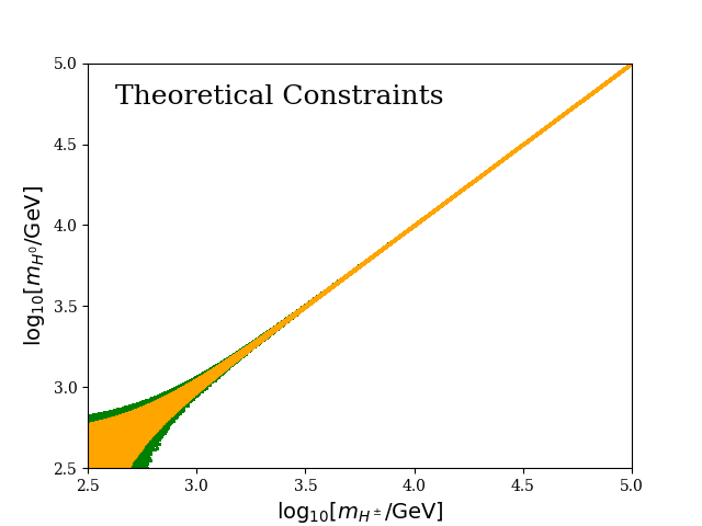
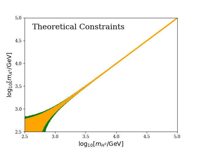
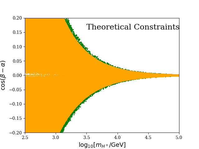
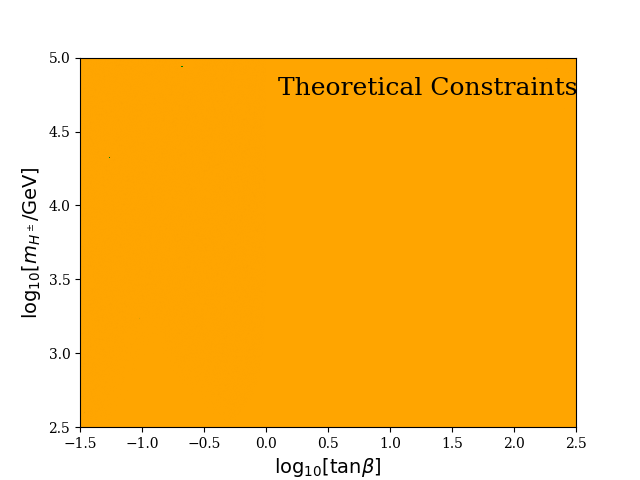
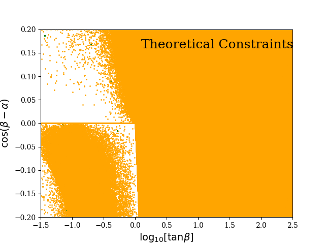
The two upper plots and the left of the middle plots of Fig. 1 show that theory constraints require the new Higgses to be more or less degenerate in mass. The heavier the mass, the stronger this requirement becomes, which can also be nicely read off from Table 1. The right plot of the middle row in Fig. 1 shows that $|\delta|$ will be constrained to small values, if the new Higgs particles are heavier than about a TeV (such a bound on the charged Higgs mass will follow from flavour constraints discussed below). Again, the constraints on $|\delta|$ become stronger the heavier the new Higgs masses become. Quantitative values for the bounds on $|\delta|$ are given in Table 1. In the lower row of Fig. 1 we see that $\tan\beta$ is not really constrained by the theory constraints, apart from the restrictions given in Eq. (22).

In the alignment limit, the value of $\alpha$ is fixed by the value of $\tan\beta$, and we find a similar requirement for a mass degeneracy of the new Higgs particles as in the general case. Moreover, we do not find any bound on $\tan\beta$ within the regions of interest.

$m_{H^{\pm}}$/TeV$\in$	$\Delta_{A^{0}H^{0}}$/GeV $\in$	$\Delta_{A^{0}H^{\pm}}$/GeV $\in$	$\Delta_{H^{0}H^{\pm}}$/GeV $\in$	$\delta\in$
$[0.0,0.5)$	$(-536,521)$	$(-420,574)$	$(-351,532)$	$(-0.5,0.5)$
$[0.5,1.0)$	$(-297,296)$	$(-328,268)$	$(-351,268)$	$(-0.5,0.5)$
$[1.0,1.5)$	$(-163,158)$	$(-123,157)$	$(-118,154)$	$(-0.30,0.25)$
$[1.5,2.0)$	$(-109,105)$	$(-74,110)$	$(-73,105)$	$(-0.19,0.16)$
$[2.0,2.5)$	$(-82,84)$	$(-52,82)$	$(-46,79)$	$(-0.14,0.13)$
$[2.5,3.0)$	$(-67,64)$	$(-42,67)$	$(-36,65)$	$(-0.11,0.09)$
$[3.0,3.5)$	$(-53,55)$	$(-35,56)$	$(-34,53)$	$(-0.09,0.08)$
$[3.5,4.0)$	$(-47,47)$	$(-30,47)$	$(-27,48)$	$(-0.07,0.07)$
$[4.0,4.5)$	$(-42,40)$	$(-30,41)$	$(-22,43)$	$(-0.07,0.06)$
$[4.5,5.0)$	$(-35,35)$	$(-23,36)$	$(-18,37)$	$(-0.06,0.06)$

Table 1: A numerical summary of the effects of imposing the theory constraints with starting values $|\lambda_{i}|<4\pi$. These intervals are found by carrying out a $10^{8}$ points Monte Carlo scan with $|\delta|<0.5$, $m_{H^{\pm}},m_{A^{0}},m_{H^{0}}<5000\,\mathrm{GeV}$ and $-1.5<\log_{10}(\tan\beta)<2.5$. We have defined $\Delta_{ij}:=m_{i}-m_{j}$.

4 Electroweak Precision Observables

The oblique parameters first proposed in Ref. Peskin:1990zt are defined as

$$S :=\frac{4e^{2}}{\alpha}\frac{d}{dq^{2}}\big{[}\Pi_{33}(q^{2})-\Pi_{3Q}(q^{2})\big{]}\big{|}_{q^{2}=0},$$ (25)

$$T :=\frac{e^{2}}{\alpha\sin^{2}(\theta_{W})m^{2}_{W}}\big{[}\Pi_{11}(0)-\Pi_{33}(0)\big{]},$$ (26)

$$U :=\frac{4e^{2}}{\alpha}\frac{d}{dq^{2}}\big{[}\Pi_{11}(q^{2})-\Pi_{33}(q^{2})\big{]}\big{|}_{q^{2}=0}.$$ (27)

$\Pi_{XY}(q^{2})$ represents the self energies of the electroweak gauge bosons $X$ and $Y$ with 4-momentum $q^{\mu}$, the subscript $i$ represents the $W_{i}$ field and the subscript $Q$ represents the $B$ field. Here we stress that in defining these oblique parameters a subtraction of the SM contributions is made; $S=S_{\rm NP}-S_{\rm SM}$ and similarly for $T$ and $U$, such that, by construction, in the SM $S=T=U=0$.

While most of the constraints we consider below depend on the particular type of the 2HDM, the oblique parameters are, at one loop order, unaffected by the Yukawa couplings and therefore universal for all 2HDMs. The expressions for $S$, $T$, and $U$ in the 2HDM (derived from Ref. Grimus:2008nb ) have been collected in Appendix C.

New physics generally has only a small effect on $U$; we therefore follow the approach outlined in Ref. Zyla:2020zbs and set $U$ to zero. This effectively reduces the error on the experimental result for $T$, due to the correlation between $T$ and $U$. The oblique parameters will be included in our global fit.

5 Higgs Signal Strengths

Signal strengths are a key measurement in determining if the observed Higgs boson is indeed that of the SM, or if new physics is involved. For a single production mode $i$ with a cross section $\sigma_{i}$, and decay channel $f$ with a branching fraction ${\cal B}_{f}$, the signal strength $\mu^{f}_{i}$ is defined as

$$\mu^{f}_{i}=\frac{(\sigma_{i}\cdotp{\cal B}_{f})_{\text{Exp.}}}{(\sigma_{i}\cdotp{\cal B}_{f})_{\text{SM}}},$$ (28)

as the cross section and branching fraction cannot be separately measured without further assumptions. Evidently if the SM is accurate, all these signal strengths should take a value of 1.

In practice, the small branching fractions and cross sections render some channels impossible to measure currently, but there are recent measurements available for 31 channels from the ATLAS and CMS collaborations at $\sqrt{s}=13\;\text{TeV}$ with an integrated luminosity of up to 139 fb^-1 and 137 fb^-1 respectively Sirunyan:2018koj ; Sirunyan:2019qia ; Aad:2019mbh ; Aad:2020plj ; Aad:2020xfq ; CMS:2020gsy ; ATLAS:2020qdt . These include various combinations of the four main $h^{0}$ production channels at the LHC: gluon-gluon fusion (ggF), vector boson fusion (VBF), in association with a weak vector boson (Vh) or a top-antitop pair (tth), and the decay channels $\gamma\gamma$, $ZZ^{*}$, $WW^{*}$, $Z\gamma$, $\tau^{+}\tau^{-}$, $b\bar{b}$ and $c\bar{c}$. The recent observations of $h^{0}\to\mu^{+}\mu^{-}$ Aad:2020xfq ; Sirunyan:2020two are also included here. In cases such as $h^{0}\to\mu^{+}\mu^{-}$ where a combined signal strength across all channels is given, it is interpreted as being purely from gluon-gluon fusion as this mechanism dominates the Higgs production cross section at the LHC. In instances where a correlation matrix between measurements is given this is also included in the analysis. For full details on which channels have been used and their experimental values, see Table LABEL:tab:List-of-Higgs-signal-strengths in Appendix A. Where multiple measurements are available for a single channel we take an average, which significantly improves our sensitivity (see flavio’s documentation for details Straub:2018kue ).

The couplings of $h^{0}$ to the massive gauge bosons and fermions are multiplied by factors $\kappa_{i}$ compared to the SM Higgs, as set out in Section 2, with the relations for $\kappa_{i}$ given in Eq. (19). As the couplings are modified, the signal strength data can be used to place constraints on the two parameters on which the $\kappa_{i}$ depend: $\cos{(\beta-\alpha)}$ and $\tan\beta$. A scenario in which

$$\kappa_{\small{V}}=1,\qquad\kappa_{u}=1,\qquad\kappa_{d,\ell}=-1,$$ (29)

has been introduced as one of the ways a fourth sequential chiral generation of fermions may still exist while remaining hidden from current LHC data Das:2017mnu . By enforcing $\kappa_{u}=-\kappa_{d}=1$ one finds

$$\cos{(\beta-\alpha)}=\sin{2\beta}=\frac{2\tan\beta}{1+\tan^{2}\beta}\,.$$ (30)

The full criteria of the wrong sign limit are satisfied exactly only when this equation is followed at very large $\tan\beta$, giving the set of couplings in Eq. (29). The contributions of the additional Higgs bosons to the loop-level processes have been neglected as they are negligible for the allowed masses found in Section 6.

Figure 2: Contour plot of the allowed 2HDM-II parameter space in the $(\tan\beta-\cos(\beta-\alpha))$ plane from the Higgs signal strengths, with the dashed black line indicating the alignment limit ($\cos(\beta-\alpha)=0$) and the dashed red line the wrong sign limit of Eq. (30). The contours indicate the allowed space at 1, 2, 3, 4, 5$\sigma$ from dark to lighter.

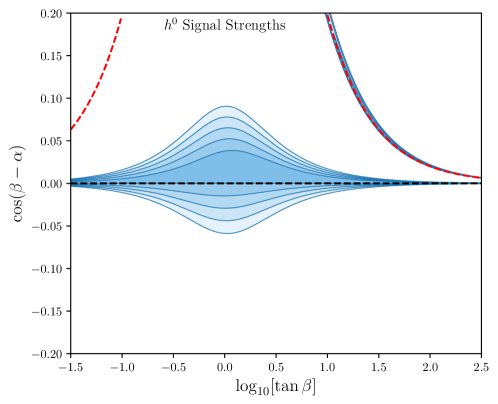
The results of the analysis including all the Higgs signal strengths listed in Table LABEL:tab:List-of-Higgs-signal-strengths are shown in Fig. 2 (see also Table 2); we will later include the Higgs signal strengths in our global fit. This fit is performed using the analytic expressions for the Higgs production and decay channels in the 2HDM found in Ref. Gunion:1989we . As outlined above, the coupling modifications, the $\kappa_{i}$, are functions of $\tan\beta$ and $\cos(\beta-\alpha)$, allowing us to constrain this plane. For some recent studies that include a similar analysis in the 2HDM, see, for instance, Refs. Chowdhury:2017aav ; Dawson:2020oco ; Han:2020zqg ; Han:2020lta ; Ellis:2018gqa . We observe that the alignment limit must be closely followed, which is unsurprising given that almost all of the experimental data included here matches the SM within 2$\sigma$, with the majority agreeing at 1$\sigma$. As a result, the 2HDM must closely replicate the SM behaviour for $h^{0}$. At 2$\sigma$ we find

$$\big{|}\cos{(\beta-\alpha)}\big{|}\leq 0.050,$$ (31)

with the maximum allowed value of $\cos{(\beta-\alpha)}$ occurring at $\tan\beta$ $\approx$ 1. Due to the dependence of $\kappa_{d,\ell}$ on $\tan\beta$, this maximum value falls significantly once away from $\tan\beta$ $\approx$ 1, to the point where, at large values of $\tan\beta$, the alignment limit must be strictly followed and it is valid to set $\cos{(\beta-\alpha)}=0$. At 3$\sigma$ and above we find the wrong sign limit to be allowed, which substantially increases this upper bound, provided Eq. (30) is closely followed.

Figure 3: Contour plot of the coupling constant modifiers, in which we have fixed to its best fit value $\kappa_{V}=1.036$ and marked the alignment (wrong-sign) limit in black (red). The contours indicate the allowed space at 1, 2, 3, 4, 5$\sigma$ from dark to lighter.

The wrong sign condition from enforcing $\kappa_{u}=-\kappa_{d}=1$, Eq. (30), which is shown in Fig. 2 as a dashed red line, is here found to be excluded at 2.7$\sigma$ by the signal strength data, an improvement over previous works such as Refs. Han:2020zqg ; Aad:2019mbh ; Bertrand:2020lyb , due in part to our inclusion of a larger data set than in such works, which improves our sensitivity.

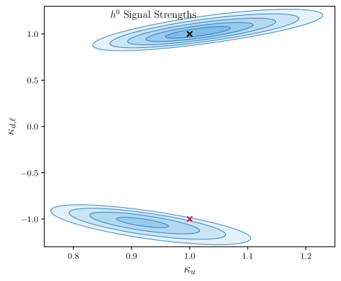
To further probe the wrong-sign limit, we examine the possible values of the coupling modification factors, independently from Eq. (19). We first perform a fit in terms of the three $\kappa_{i}$ to find the best fit point, and then fix one of the $\kappa_{i}$ to its best fit value, allowing a 2D fit in terms of the remaining $\kappa_{j,k\neq i}$ to be performed. We show the results from such a fit in the $(\kappa_{u}-\kappa_{d,\ell})$ plane in Fig. 3, where we have fixed to the best fit value $\kappa_{V}=1.036$, and stress again that these results do not make use of Eq. (19). This fit does not exclude $\kappa_{d}=-1$, in line with the current lack of sensitivity to the sign of $\kappa_{d}$ at the LHC. We then look to find solutions in terms of $\tan\beta$ and $\cos(\beta-\alpha)$ that give values of $\kappa_{u}$ and $\kappa_{d}$ that lie within the 2$\sigma$ allowed region close to $\kappa_{d}=-1$ (bottom part of Fig. 3) by using Eq. (19). However, the only solutions we find require that $|\cos(\beta-\alpha)|\gtrsim 0.96$. Such extreme values of $\cos(\beta-\alpha)$ are not consistent, in the 2HDM-II, with the fixed value of $\kappa_{V}=1.036$ from the best fit point that we use in the scan. Therefore this $2\sigma$ allowed region in the $(\kappa_{u}-\kappa_{d,\ell})$ plane cannot be attained in the 2HDM-II. Thus, while we do not in general exclude $\kappa_{d}=-1$ we can, in the 2HDM-II that we examine here, rule out the arrangement $\kappa_{u}=-\kappa_{d}=1$ (given by Eq. (30)) at 2.7$\sigma$ from Fig. 2.

More generally, we observe that when $\kappa_{d,\ell}=-1$, small deviations away from $\kappa_{u}=1$ have a significant impact, causing $\cos(\beta-\alpha)$ to be large, which is incompatible with the signal strength data. The debate in the literature over the possibility of the wrong-sign limit will hopefully be resolved by future collider data, with suggestions on fruitful search channels made in Refs. Modak:2016cdm and Raju:2020hpe , with the latter also including the possibility of a hidden sequential fourth generation of fermions.

6 Flavour Observables

In this section, we present our fits of the 2HDM-II for selected flavour observables. We show fits for groups of observables individually, and then in Section 7, we combine these with all other observables in the global fit. For each fit, we use the standard $(\tan\beta-m_{H^{+}})$ parameter space in a log-log scale. All fits have been performed using the flavio package as described in Section 1.

6.1 Leptonic and Semi-leptonic Tree-Level Decays

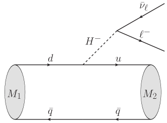
The Yukawa term in the 2HDM-II Lagrangian (17) leads to additional contributions to the tree-level flavour-changing charged transitions. Integrating out the heavy charged Higgs boson $H^{\pm}$, one obtains the effective Hamiltonian describing the $d\to u\,\ell^{-}\bar{\nu}_{\ell}$ or $u\to\,d\ell^{+}\nu_{\ell}$ transition in the 2HDM:

$${\cal H}^{\rm eff}_{H^{+}}=-\frac{4G_{F}}{\sqrt{2}}V_{ud}(C_{S-P}\,{\cal O}_{S-P}+C_{S+P}\,{\cal O}_{S+P})+{\rm h.c.,}$$ (32)

where the new effective operators are

$$\mathcal{O}_{S-P}=(\bar{u}P_{L}\,d)(\bar{\ell}P_{L}\nu_{\ell}),\qquad\mathcal{O}_{S+P}=(\bar{u}P_{R}\,d)(\bar{\ell}P_{L}\nu_{\ell}).$$ (33)

The corresponding Wilson coefficients are related to the 2HDM-II parameters as follows:

$$C_{S-P}=\frac{m_{u}\,m_{\ell}}{m_{H^{+}}^{2}}\,,\qquad C_{S+P} =\frac{m_{d}\,m_{\ell}\tan^{2}\beta}{m_{H^{+}}^{2}}\,.$$ (34)

For use in flavio, we convert the latter coefficients to $C_{SL}^{du\ell\nu_{\ell}},C_{SR}^{du\ell\nu_{\ell}}$, respectively, in the flavio WET basis, finding

$$C_{SL}^{du\ell\nu_{\ell}}=-C_{S-P}\,,\qquad C_{SR}^{du\ell\nu_{\ell}} =-C_{S+P}\,,$$ (35)

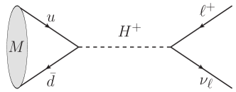
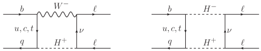
where the negative sign in front of these coefficients is due to the convention for the effective operators adopted in flavio’s basis. Feynman diagrams describing the leptonic and semi-leptonic transitions in the 2HDM are shown in Fig. 4.

Figure 4: Diagrams contributing to leptonic (left) and semi-leptonic (right) decays in the 2HDM.

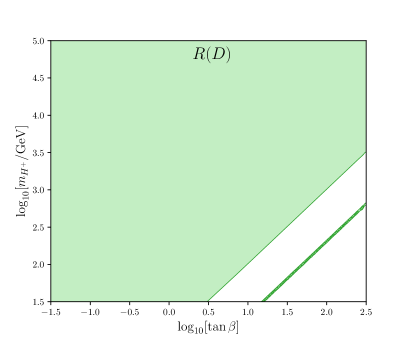
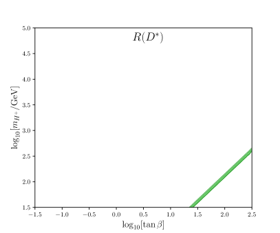
The full list of leptonic and semi-leptonic modes included in our fit is given in Table LABEL:tab:List-of-flavour-observables, where the corresponding SM predictions (produced in flavio) are based on Bernlochner:2017jka ; Caprini:1997mu ; Sakaki:2013bfa ; Bharucha:2015bzk ; Gubernari:2018wyi ; Detmold:2016pkz ; Bernard:2006gy ; Bernard:2009zm ; Antonelli:2010yf . In addition to previously measured semi-leptonic decay channels, we consider for the first time the $B_{s}\to D_{s}^{(*)}\mu\bar{\nu}_{\mu}$ modes measured recently by the LHCb collaboration Aaij:2020hsi , and the corresponding $B_{s}\to D_{s}^{(*)}$ form factors are determined using Lattice QCD McLean:2019qcx . Moreover, we consider the Lepton-Flavour Universality (LFU) observables $R(D^{(*)})\equiv{\cal B}(B\to D^{(*)}\tau\bar{\nu}_{\tau})/{\cal B}(B\to D^{(*)}\ell\bar{\nu}_{\ell})$, where $\ell=e$ or $\mu$. The experimental measurements of the latter were found to be in tension with the corresponding SM predictions, giving hints of possible LFU violation. In the 2HDM, this violation is caused by different couplings of the charged Higgs boson to the lepton pair, which are proportional to the lepton mass $m_{\ell}$. Using the HFLAV averages for $R(D^{(*)})$ Amhis:2019ckw , we present in Fig. 5 the allowed $(\tan\beta-m_{H^{+}})$ regions at 1 and 2$\sigma$ levels, where the left (right) plot corresponds to $R(D)$ ($R(D^{*})$). Note that the semi-leptonic $b\to c\ell\bar{\nu}_{\ell}$ transitions receive negative corrections compared to the SM contributions, therefore $R(D)$ and $R(D^{*})$ move further away from the measurements (apart from a narrow region of the $(\tan\beta-m_{H^{+}})$ parameter space (see Fig. 5), where the 2HDM-II correction becomes more than the twice the size of the SM contribution proportional to the scalar form factor). Since $R(D)$ is in fact only $1.2\sigma$ away from the SM prediction (see Table LABEL:tab:List-of-flavour-observables), one finds a wide allowed range of $\tan\beta$ and $m_{H^{+}}$ at the $2\sigma$ level (the left plot in Fig. 5). On the other side, $R(D^{*})$ is in greater tension ($2.8\sigma$) with the SM, therefore one obtains just a narrow region with large $\tan\beta$ and small $m_{H^{+}}$ (the right plot in Fig. 5). The experimental combination of both $R(D)$ and $R(D^{*})$ Amhis:2019ckw is more than three standard deviations away from the SM prediction, and within 2$\sigma$ one finds in the 2HDM-II only a very narrow region at very low masses of the charged Higgs, $m_{H^{+}}\sim 1\,{\rm GeV}$, which is far from the physical domain. We find that the 2HDM-II is not able to accommodate the experimental data on both $R(D)$ and $R(D^{*})$ within $3.5\,\sigma$; the corresponding tension in the SM (using flavio) is $3.2\,\sigma$.

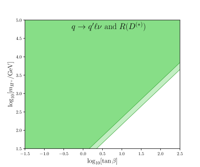
Combining all the leptonic and semi-leptonic tree-level decay channels indicated in Table LABEL:tab:List-of-flavour-observables yields the allowed range of $\tan\beta$ and $m_{H^{+}}$ at $1$ and $2\sigma$ levels as shown in Fig. 6.

Figure 5: Contour plot of the allowed 2HDM-II parameter space in the $(\tan\beta-m_{H^{+}})$ plane, originating from $R(D)$ (left) and $R(D^{*})$ (right). The lighter contour indicates the allowed parameter space at $2\sigma$ confidence level while the darker contour corresponds to $1\sigma$.

Figure 6: Contour plot of the allowed 2HDM-II parameter space in the $(\tan\beta-m_{H^{+}})$ plane, originating from the combination of tree-level leptonic and semi-leptonic decays of $B,B_{s},D,D_{s},K$, and $\pi$ mesons and the hadronic decays of $\tau$ leptons to $K$ and $\pi$ mesons with a tau neutrino as well as $R(D)$ and $R(D^{*})$, see Table LABEL:tab:List-of-flavour-observables. The lighter contour indicates the allowed parameter space at $2\sigma$ confidence level while the darker contour corresponds to $1\sigma$.

In addition, we would like to make an important observation regarding the extraction of the CKM matrix elements from experimental data. Consider e.g. the branching fraction of a leptonic meson decay in the 2HDM,

$$\mathcal{B}_{\rm 2HDM}=\mathcal{B}_{\rm SM}\times(1+\delta_{\rm 2HDM})^{2},$$ (36)

where $\delta_{\rm 2HDM}$ is the 2HDM correction factor. Conventionally, the corresponding CKM element is determined from the experimental measurement, assuming $\mathcal{B}_{\rm exp}=\mathcal{B}_{\rm SM}$. But if the 2HDM is realistic then $\mathcal{B}_{\rm exp}=\mathcal{B}_{\rm 2HDM}$ and the CKM element extracted from measurement is actually proportional to $(1+\delta_{\rm 2HDM})$. Therefore, the fraction $1/(1+\delta_{\rm 2HDM})$ is then interpreted as the modification factor that the measured CKM element must receive in the 2HDM to be the true CKM element. A similar argument holds for the semi-leptonic meson decays.

Using Eq. (36), and a similar relation for the semi-leptonic decays, the size of the modification factor $1/(1+\delta_{\rm 2HDM})$ can be scanned across the 2HDM-II parameter space $(\tan\beta-m_{H^{+}})$ to test the significance of the factor for each of the CKM matrix elements, where the accepted values are commonly taken from leptonic and semi-leptonic tree-level decays. We perform tests of this significance for $V_{us}$, $V_{ub}$ and $V_{cb}$ using the tree-level parameterisation to consider the propagated effects to all CKM elements, and we also take into account unitarity of the CKM matrix. We find negligible effects to all CKM elements for most of the parameter space considered here, and the small areas where more noticeable effects arise are excluded from theoretical constraints, direct searches, and by the global fit in Section 7.

Were the 2HDM-II proven to be physical, it could be the case that there is some small modification to CKM elements that, although is not enough to impact results here, would need to be considered. This would be dependent on the specific values found for $m_{H^{+}}$ and $\tan\beta$ from experiment.

6.2 Neutral $B$-Meson Mixing

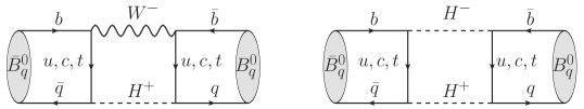
Neutral $B$-meson mixing plays an important role in flavour physics. For a recent discussion on $B$-mixing in the SM and within New Physics models see, for example, Ref. DiLuzio:2019jyq . In the 2HDM, $B$-mixing gains additional contributions from new box diagrams where one or both of the virtual $W^{\pm}$ bosons are replaced by charged Higgses $H^{\pm}$, see Fig. 7. Here we consider the mass difference $\Delta m_{d,s}$ between the heavy and light eigenstates in both $B_{d}$ and $B_{s}$ meson mixing.

Figure 7: Examples of box diagrams describing $B_{d}$- and $B_{s}$-meson mixing in the 2HDM.

The effective 2HDM Hamiltonian for $\Delta B=2$ processes can be expressed as Crivellin:2019dun :

$$\mathcal{H}_{\rm eff}^{\Delta B=2}=\sum_{k=1}^{5}C_{k}\mathcal{O}_{k}+\sum_{k=1}^{3}C_{k}^{\prime}\mathcal{O}_{k}^{\prime},$$ (37)

where the operators are defined (for $q=d,s$) as

$$\mathcal{O}_{1}^{(^{\prime})} =(\bar{q}^{\alpha}\gamma^{\mu}P_{L(R)}b^{\alpha})(\bar{q}^{\beta}\gamma_{\mu}P_{L(R)}b^{\beta}),$$ (38)

$$\mathcal{O}_{2}^{(^{\prime})} =(\bar{q}^{\alpha}P_{L(R)}b^{\alpha})(\bar{q}^{\beta}P_{L(R)}b^{\beta}), \mathcal{O}_{4} =(\bar{q}^{\alpha}P_{L}b^{\alpha})(\bar{q}^{\beta}P_{R}b^{\beta}),$$

$$\mathcal{O}_{3}^{(^{\prime})} =(\bar{q}^{\alpha}P_{L(R)}b^{\beta})(\bar{q}^{\beta}P_{L(R)}b^{\alpha}), \mathcal{O}_{5} =(\bar{q}^{\alpha}P_{L}b^{\beta})(\bar{q}^{\beta}P_{R}b^{\alpha}),$$

with $\alpha$ and $\beta$ denoting the colour indices. The contributions of these operators to $B$-meson mixing in the 2HDM are well-known throughout literature, see e.g. Refs. Geng:1988bq ; Urban:1997gw ; Crivellin:2019dun . In our work, for the Wilson coefficients $C^{(\prime)}_{k}$ in Eq. (37) we use expressions calculated in Ref. Crivellin:2019dun . We convert these to the flavio WET basis Aebischer:2017ugx , where we find

$$C_{VLL(RR)}^{bqbq} =C_{1}^{(^{\prime})}, \qquad C_{SLR}^{bqbq} =C_{4},$$ (39)

$$C_{SLL(RR)}^{bqbq} =C_{2}^{(^{\prime})}, C_{VLR}^{bqbq} =-\frac{1}{2}\,C_{5}.$$

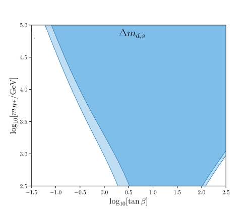
The operators $\mathcal{O}_{3}^{(^{\prime})}$ do not give any contributions (at LO in QCD) to mixing in the 2HDM Crivellin:2019dun , so we do not need to consider conversion for $C_{3}^{(\prime)}$ here. The largest theory uncertainties by far stem from the non-perturbative values of the matrix elements of the $\Delta B=2$ operators given in Eq. (38). In our analysis we will use the averages presented in Ref. DiLuzio:2019jyq , which are based on HQET Sum Rule evaluations King:2019lal ; Kirk:2017juj ; Grozin:2016uqy and lattice simulations Dowdall:2019bea ; Boyle:2018knm ; Bazavov:2016nty . The perturbative SM corrections are known and implemented to NLO-QCD accuracy Buras:1990fn . In the numerical analysis we further use the most recent experimental averages for $\Delta m_{d}$ and $\Delta m_{s}$ Amhis:2019ckw (see Table LABEL:tab:List-of-flavour-observables). The results of the fit are shown in Fig. 8, indicating that the mass differences constrain the allowed $\tan\beta$ region from below.

Figure 8: Contour plot of the allowed 2HDM-II parameter space in the $(\tan\beta-m_{H^{+}})$ plane for the mass difference in the mixing of $B_{d}$ and $B_{s}$ mesons. The lighter contour indicates the allowed parameter space at $2\sigma$ confidence level while the darker contour corresponds to $1\sigma$.

6.3 Loop-Level $b\to s,d$ Transitions

The effective Hamiltonian for flavour-changing neutral current (FCNC) $b\to q\ell^{+}\ell^{+}$ and $b\to s\gamma$ (for $q=d,s$) processes is defined as Crivellin:2019dun

$$\mathcal{H}_{\rm eff}^{b\to q\ell\ell}=-\frac{4G_{F}}{\sqrt{2}}V_{tb}V_{tq}^{*}\left(\sum_{k=7,8}C_{k}^{(^{\prime})}\mathcal{O}_{k}^{(^{\prime})}+\sum_{k=9,10,S,P}\!\!\!C_{k}^{(^{\prime})}\mathcal{O}_{k}^{(^{\prime})}\right)+{\rm h.c.}.$$ (40)

The operators in this Hamiltonian are

$$\mathcal{O}_{7}^{(^{\prime})} =\frac{e\,m_{b}}{16\pi^{2}}\left(\bar{q}\sigma^{\mu\nu}P_{R(L)}b\right)\!F_{\mu\nu}, \mathcal{O}_{8}^{(^{\prime})} =\frac{g_{s}\,m_{b}}{16\pi^{2}}\left(\bar{q}\sigma^{\mu\nu}P_{R(L)}T^{a}b\right)\!G_{\mu\nu}^{a},$$ (41)

$$\mathcal{O}_{9}^{(^{\prime})} =\frac{e^{2}}{16\pi^{2}}(\bar{q}\gamma_{\mu}P_{L(R)}b)(\bar{\ell}\gamma^{\mu}\ell), \mathcal{O}_{10}^{(^{\prime})} =\frac{e^{2}}{16\pi^{2}}(\bar{q}\gamma_{\mu}P_{L(R)}b)(\bar{\ell}\gamma^{\mu}\gamma_{5}\ell),$$

$$\mathcal{O}_{S}^{(^{\prime})} =\frac{e^{2}}{16\pi^{2}}(\bar{q}P_{L(R)}b)(\bar{\ell}\ell), \mathcal{O}_{P}^{(^{\prime})} =\frac{e^{2}}{16\pi^{2}}(\bar{q}P_{L(R)}b)(\bar{\ell}\gamma_{5}\ell).$$

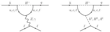
The expressions for 2HDM-II contributions to each operator’s Wilson coefficient are given e.g. in Section 3 of Crivellin:2019dun . Since all the operators in Eq. (40) are defined in the same way as in the flavio WET basis (for either $\ell=e,\mu$), no Wilson coefficient conversions are required here. Some example diagrams describing the $b\to q\ell^{+}\ell^{-}$ transitions in the 2HDM are shown in Fig. 9.

Figure 9: Example of diagrams (penguins and boxes) describing the $b\to q\ell^{+}\ell^{-}$ transitions in the 2HDM.

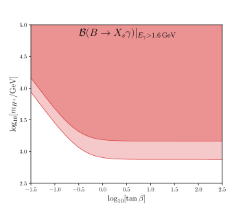
6.3.1 Radiative Decay $\bar{B}\to X_{s}\gamma$

Figure 10: One-loop penguin contributions to $b\to s\gamma$ processes in the 2HDM.

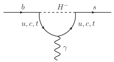
The radiative decay $\bar{B}\to X_{s}\gamma$ is an important observable in the 2HDM-II. Historically, it has played a significant role in giving a lower bound on the charged Higgs mass. A recent update of the SM value with NNLO accuracy in QCD Misiak:2020vlo (based on e.g. Refs. Misiak:2006ab ; Misiak:2015xwa ),

$$\mathcal{B}^{\rm SM}(\bar{B}\to X_{s}\gamma)\big{|}_{E_{\gamma}>1.6\,{\rm GeV}}=(3.40\pm 0.17)\times 10^{-4},$$ (42)

leads to a stronger constraint on the charged Higgs mass: $m_{H^{+}}\geq 800\,$GeV (95% CL) Misiak:2020vlo . The experimental average from Amhis:2019ckw is based on Chen:2001fja ; Lees:2012ym ; Belle:2016ufb . The operators which contribute to the radiative decays $\bar{B}\to X_{s}\gamma$ are $\mathcal{O}_{7},\mathcal{O}_{8}$, given by Eq. (41). As expected, our fit for this process provides an important lower bound for the charged Higgs mass, predicted here as (see also Fig. 11)

$$m_{H^{+}}\gtrsim 790\,(1510)\,\text{GeV}\;\text{ at }2\sigma\,(1\sigma).$$ (43)

We slightly differ from Ref. Misiak:2020vlo in that our 2HDM-II contributions are taken at NLO Borzumati:1998nx , while they use NNLO results Hermann:2012fc and we also use a different statistical treatment. In addition, as can be seen in Fig. 11, the bound for $m_{H^{\pm}}$ becomes even stronger for lower values of $\tan\beta$.

Figure 11: Contour plot of the allowed 2HDM-II parameter space in the $(\tan\beta-m_{H^{+}})$ plane for the radiative decay $B\to X_{s}\gamma$. The lighter contour indicates the allowed parameter space at $2\sigma$ confidence level while the darker contour corresponds to $1\sigma$.

6.3.2 Leptonic $B_{d,s}\to\mu^{+}\mu^{-}$ Decays

The FCNC leptonic meson decays $B_{d,s}\to\mu^{+}\mu^{-}$ are particularly sensitive to scalar operator contributions in NP models, and therefore can be excellent probes of the effects of the 2HDM. These processes are particularly worthy of consideration now, due to the recently-produced experimental combinations which we use in our fit Altmannshofer:2021qrr , and recent ATLAS, CMS, and LHCb results Aaij:2017vad ; Aaboud:2018mst ; Sirunyan:2019xdu ; LHCb-CONF-2020-002 ; LHCb:2021awg ; LHCb:2021vsc . The SM prediction is based on a perturbative element Buchalla:1993bv ; Bobeth:2013uxa ; Beneke:2019slt and a non-perturbative determination of the decay constants, see e.g. Ref. Bussone:2016iua ; Bazavov:2017lyh ; Hughes:2017spc . It has been common in the past to study these decays in the large $\tan\beta$ limit ($\tan\beta\gg\sqrt{m_{t}/m_{b}}$, see e.g. Ref. Logan:2000iv ) where the Yukawa coupling to $b$ quarks is large and there can be simplifications to the 2HDM contributions of the operators which affect this process: $\mathcal{O}_{10}^{(^{\prime})},\mathcal{O}_{S}^{(^{\prime})},\mathcal{O}_{P}^{(^{\prime})}$. However, a big part of the allowed parameter space of the 2HDM-II lies not within the large $\tan\beta$, thus we use only the general expressions given in Ref. Crivellin:2019dun .

Figure 12: Contour plot of the allowed 2HDM-II parameter space in the $(\tan\beta-m_{H^{+}})$ plane for the FCNC leptonic $B_{d,s}\to\mu^{+}\mu^{-}$ decays, fixing the additional parameters as $\cos(\beta-\alpha)=0$, $m_{H^{0}}=m_{A^{0}}=m_{H^{+}}$. The lighter contour indicates the allowed parameter space at $2\sigma$ confidence level while the darker contour corresponds to $1\sigma$.

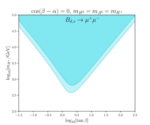
These generalised expressions bring three further parameters of the 2HDM into play: $\alpha$, $m_{H^{0}}$, and $m_{A^{0}}$. In Section 7, we will combine all observables in a fit of the five independent parameters: $\tan\beta$, $m_{H^{+}}$, $m_{H^{0}}$, $m_{A^{0}}$ and $\cos(\beta-\alpha)$. Here, in order to present a 2D fit in the $(\tan\beta-m_{H^{+}})$ parameter space, we fix the other three parameters as $\cos(\beta-\alpha)=0$, as the alignment limit is preferred (see Section 7) by the global fit, and $m_{H^{0}}=m_{A^{0}}=m_{H^{+}}$, which is justified from theoretical constraints (see Section 3). The corresponding contour plot is shown in Fig. 12. From there one can see that the mass of charged Higgs is also constrained from below, roughly:

$$m_{H^{+}}\gtrsim 300\,{\rm GeV},$$ (44)

however this bound is not as strong as that from the $B\to X_{s}\gamma$ decay. Furthermore, $B_{d,s}\to\mu^{+}\mu^{-}$ yields a strong correlation between possible values of $\tan\beta$ and $m_{H^{+}}$.

6.3.3 Semi-leptonic $b\to s\ell^{+}\ell^{-}$ Transitions

For the semi-leptonic $b\to s\ell^{+}\ell^{-}$ processes we are considering, all of the operators from Eq. (41) contribute. Therefore all the 2HDM parameters, $m_{H^{+}}$, $m_{H^{0}}$, $m_{A^{0}}$, $\tan\beta$ and $\cos(\beta-\alpha)$, will affect these processes.

The first group of observables are the LFU ratios $R_{K}$ and $R_{K^{*}}$ Bobeth:2007dw , defined as

$$R_{K^{(*)}}\equiv\frac{\mathcal{B}[B\to K^{(*)}\mu^{+}\mu^{-}]}{\mathcal{B}[B\to K^{(*)}e^{+}e^{-}]},$$ (45)

where the branching fractions are integrated over bins of squared dilepton invariant mass $q^{2}$. These quantities are theoretically very clean, since almost all hadronic effects drop out in the ratio. In the SM, the values of $R_{K^{(*)}}$ are very close to 1 with tiny uncertainties. The electromagnetic corrections for $R_{K^{(*)}}$ worked out in Ref. Bordone:2016gaq were found to be very small, $\approx 1-2\%$. In our analysis, we consider the ten binned LFU ratios listed in Table LABEL:tab:RKtab. The recent measurement by LHCb shows a deviation from the SM of $3.1\sigma$ for $R_{K^{+}}$ Aaij:2021vac .

Figure 13: Contour plot of the allowed 2HDM-II parameter space in the $(\tan\beta-m_{H^{+}})$ plane for the $R_{K^{(*)}}$ observables and fixing the additional parameters at their best fit point in Table 2. The lighter contour indicates the allowed parameter space at $2\sigma$ confidence level while the darker contour corresponds to $1\sigma$.

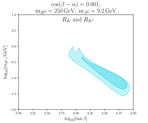
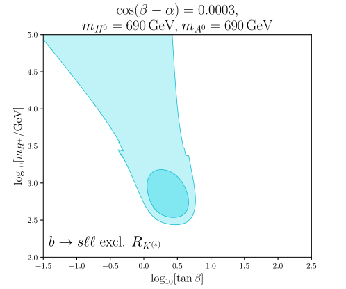
In Fig. 13 we present the resulting $(\tan\beta-m_{H^{+}})$ contour plot for $R_{K^{(*)}}$ observables, where we fixed the three other 2HDM parameters at their best fit values for the 10 $R_{K^{(*)}}$ bins: $\cos(\beta-\alpha)=0.001$, $m_{H^{0}}=250\,{\rm GeV},m_{A^{0}}=9.2\,$ GeV (see Table 2). As one can see, $R_{K^{(*)}}$ could only be accommodated within the 2HDM-II only at very low $m_{H^{+}}\lesssim 1\,{\rm GeV}$ and very high $\tan\beta\gtrsim 300$, which are beyond the physical domain (see Section 3). Therefore, the 2HDM-II (as well as the SM) is unable to accommodate the current experimental values of $R_{K^{(*)}}$. The contours in Fig. 13 are not only found in regions which are in disagreement with the allowed contours in Figs. 6, 8, 11, 12, but also with the constraints from direct searches Aaboud:2018gjj . Moreover, in deriving the formulae for the relevant Wilson coefficients Crivellin:2019dun , it was assumed that $m_{H^{+}}$ is at least of the order of the electroweak scale, meaning that the validity of contours much lower than $\log_{10}[m_{H^{+}}/\text{GeV}]\sim 2$ must be questioned.

The combined fit of the 10 $R_{K^{(*)}}$ observables is in disagreement with our combined fits of all observables to $4.2\,\sigma$ confidence. Due to this disagreement between $R_{K^{(*)}}$ and other flavour observables, we work with two approaches for our fits: excluding and including $R_{K^{(*)}}$.

Next we include further $b\to s\ell^{+}\ell^{-}$ observables (binned branching ratios, angular distributions, asymmetries, etc.) – some of these also deviate from the SM predictions, see Table LABEL:tab:bsll. For more detailed analyses of these processes and their NP implications, see e.g. Refs. Khodjamirian:2010vf ; Khodjamirian:2012rm ; Bharucha:2015bzk ; Khodjamirian:2017fxg ; Alguero:2019ptt ; Hurth:2020ehu ; Alok:2019ufo ; Ciuchini:2019usw ; Hurth:2020rzx ; Hurth:2021nsi ; Alguero:2021anc ; Cornella:2021sby ; Altmannshofer:2021qrr ; Geng:2021nhg ; Ciuchini:2020gvn ; MunirBhutta:2020ber ; Biswas:2020uaq . For all $b\to s\ell^{+}\ell^{-}$ processes listed in Table LABEL:tab:bsll and the leptonic decays $B_{q}\to\mu^{+}\mu^{-}$ (see Table LABEL:tab:List-of-flavour-observables), but excluding the $R_{K^{(*)}}$ observables, one gets the allowed regions for $\tan\beta$ and $m_{H^{+}}$ shown in Fig. 14. Deviations of experiment from SM predictions now introduce an upper bound on the charged Higgs mass at $1\sigma$. A further inclusion of the $R_{K^{(*)}}$ observables does not change the contours of allowed regions in Fig. 14 sizeably, but does worsen the corresponding fit and the $p$-value, see Table 2.

Figure 14: Contour plot of the allowed 2HDM-II parameter space in the $(\tan\beta-m_{H^{+}})$ plane for the leptonic $B_{d,s}\to\mu^{+}\mu^{-}$ decays and the semi-leptonic $b\to s\ell^{+}\ell^{-}$ observables listed in Table LABEL:tab:bsll excluding the $R_{K^{(*)}}$ observables and fixing the additional parameters to the best fit point from the $b\to s\ell^{+}\ell^{-}$ fit in Table 2. The lighter contour indicates the allowed parameter space at $2\sigma$ confidence level while the darker contour corresponds to $1\sigma$.

7 Global Fit

7.1 Results

Combining all the observables collected in Table LABEL:tab:List-of-Higgs-signal-strengths (Higgs signal strengths), Table LABEL:tab:List-of-oblique-parameters ($S,T,U$), Table LABEL:tab:List-of-flavour-observables (flavour observables without $b\to s\ell^{+}\ell^{-}$), Table LABEL:tab:bsll ($b\to s\ell^{+}\ell^{-}$ observables) and Table LABEL:tab:RKtab ($R_{K^{(*)}}$) one obtains the results shown in Table 2. We emphasize that in searching for the best-fit point of the corresponding likelihood function we have applied the theory constraints for the Higgs mass differences (see Table 1). As one can see from Table 2, including all the observables yields a relatively poor fit with a low $p\approx 1.5\%$-value. This is due to the fact that the $R_{K^{(*)}}$ and $R(D^{(*)})$ quantities cannot be accommodated within the 2HDM-II, as was already discussed in Sections 6.1 and 6.3.3. Nevertheless the 2HDM-II still achieves a higher level of agreement than the SM and we find a corresponding pull of $2.3\sigma$. Not considering the observables $R_{K^{(*)}}$ yields a better fit for the 2HDM-II with a significantly higher $p\approx 7\%$-value, again marking a better performance than the SM, with a corresponding pull of $1.8\sigma$.

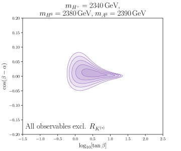
Next we find from Table 2 and Fig. 15 that the global fit prefers the alignment limit, $\cos(\beta-\alpha)=0$, allowing only small deviations from zero:

$$\max\{|\cos(\beta-\alpha)|\}\leq 0.02\,(0.04),\qquad{\rm at}\,\,1\sigma\,(2\sigma).$$ (46)

This bound is considerably stronger than the one we obtained in Eq. (31) using only data on Higgs signal strengths. Regarding the wrong sign limit solution, we found using only the Higgs signal strengths this to be allowed at $2.7\sigma$ or above; using the global fit of all observables (excluding $R_{K^{(*)}}$), this is now excluded within $6\sigma$ of our best fit point with $p$-value $\approx 7\%$. We also perform fits to all observables requiring the wrong sign limit as defined in Eq. (30), where one can see the quality of these fits is significantly worsened compared to the general global fit with no input constraint on $\cos(\beta-\alpha)$, yielding a $p$-value $\approx 0.1\%$.

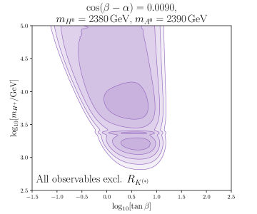
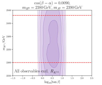
The best fit further favours values of $m_{H^{+}}\approx m_{H^{0}}\approx m_{A^{0}}\approx 2.3$ TeV and $\tan\beta\approx 4$. Performing a scan around the best-fit point (excluding $R_{K^{(*)}}$) and keeping in mind the theory constraints in Table 2, we find that the charged Higgs mass is constrained to be in the region

$$76.3\,{\rm TeV}\geq m_{H^{+}}\geq 1.26\,{\rm TeV} \mbox{at }1\sigma,$$

$$m_{H^{+}}\geq 0.86\,{\rm TeV} \mbox{at }2\sigma,$$

$$m_{H^{+}}\geq 0.68\,{\rm TeV} \mbox{at }3\sigma,$$

$$m_{H^{+}}\geq 0.57\,{\rm TeV} \mbox{at }4\sigma,$$

$$m_{H^{+}}\geq 0.49\,{\rm TeV} \mbox{at }5\sigma.$$ (47)

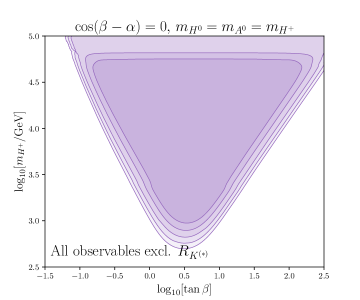
From the $2\sigma$-level onwards we do not see an upper bound within the area considered ($m_{H^{+}}\leq 100\,{\rm TeV}$). The parameter $\tan\beta$ has a strong correlation with $m_{H^{+}}$. For the best fit values of $\cos(\beta-\alpha)$, $m_{H^{0}}$ and $m_{A^{0}}$, we find the allowed regions in the ($\tan\beta-m_{H^{+}}$) plane given in Fig. 16 and Fig. 17 (the latter zoomed into the best-fit point and shown in combination with the theory constraints). Assuming both the alignment limit, $\cos(\beta-\alpha)=0$, and the degeneracy for the Higgs masses, $m_{H^{+}}=m_{H^{0}}=m_{A^{0}}$, the contour plot of Fig. 18 shows that $\tan\beta$ is strongly constrained for low $m_{H^{+}}\sim 1\,{\rm TeV}$ while the bounds on $\tan\beta$ become weaker with an increase of $m_{H^{+}}$ up to $100\,{\rm TeV}$. We stress again that these constraints above are obtained from the fit by excluding $R_{K^{(*)}}$. The inclusion of $R_{K^{(*)}}$ would not significantly change the allowed parameter regions, while it would considerably worsen the quality of the fit.

Furthermore, we investigate several constrained scenarios in the fit, as indicated in Table 2. First, we checked that the wrong-sign limit is absolutely disfavored by the global fit. Second, in the exact alignment limit the fit yields similar results as in the general case. Finally, assuming both the alignment limit, $\cos(\beta-\alpha)=0$, and the degeneracy for the Higgs masses, $m_{H^{+}}=m_{H^{0}}=m_{A^{0}}$, again leads to similar results due to the preference of both of these assumptions by the global fit and theory constraints.

Scenario	$\#$	Best-fit point	$\chi_{min}^{2}$	$p$-value
	Observables	$\{\tan\beta,m_{H^{+}},m_{H^{0}},m_{A^{0}},\cos(\beta-\alpha)\}$
All incl. $R_{K^{(*)}}$	$275$	$\{4.2,2140\,{\rm GeV},2180\,{\rm GeV},2210\,{\rm GeV},0.0096\}$	$323$	$\phantom{0}1.5\%$
All excl. $R_{K^{(*)}}$	$265$	$\{4.3,2340\,{\rm GeV},2380\,{\rm GeV},2390\,{\rm GeV},0.0090\}$	$295$	$\phantom{0}6.6\%$
Flavour incl. $R_{K^{(*)}}$	$241$	$\{4.2,2310\,{\rm GeV},2300\,{\rm GeV},2290\,{\rm GeV},0.001\}$	$297$	$\phantom{0}0.4$%
Flavour excl. $R_{K^{(*)}}$	$231$	$\{4.3,2420\,{\rm GeV},2390\,{\rm GeV},2360\,{\rm GeV},0.0001\}$	$269$	$\phantom{0}2.5$%
$b\to s\ell\ell$ incl. $R_{K^{(*)}}$	$202$	$\{4.0,820\,{\rm GeV},690\,{\rm GeV},690\,{\rm GeV},0.0003\}$	$265$	$\phantom{0}0.1$%
$b\to s\ell\ell$ excl. $R_{K^{(*)}}$	$192$	$\{4.0,820\,{\rm GeV},690\,{\rm GeV},690\,{\rm GeV},0.0003\}$	$238$	$\phantom{0}0.7$%
Only $R_{K^{(*)}}$	$10$	$\{2370,0.14\,{\rm GeV},250\,{\rm GeV},9.2\,{\rm GeV},0.001\}$	$8.5$	$13.1$%
Higgs Signals	$31$	$\{\sim 100\pm 20,-,-,-,0.0003\}$	$24$	$72.9$%
Wrong Sign Limit, $\cos(\beta-\alpha)=\sin 2\beta$
All incl. $R_{K^{(*)}}$	$275$	$\{12.1,2320\,{\rm GeV},2270\,{\rm GeV},2260\,{\rm GeV}\}$	$380$	$0.001\%$
All excl. $R_{K^{(*)}}$	$265$	$\{12.2,2320\,{\rm GeV},2270\,{\rm GeV},2260\,{\rm GeV}\}$	$340$	$0.1\%$
Alignment Limit, $\cos(\beta-\alpha)=0$
All incl. $R_{K^{(*)}}$	$275$	$\{4.1,2290\,{\rm GeV},2330\,{\rm GeV},2340\,{\rm GeV}\}$	$326$	$1.3$%
All excl. $R_{K^{(*)}}$	$265$	$\{4.2,2260\,{\rm GeV},2300\,{\rm GeV},2310\,{\rm GeV}\}$	$297$	$6.4$%
$\cos(\beta-\alpha)=0$, $m_{H^{+}}=m_{H^{0}}=m_{A^{0}}$
All incl. $R_{K^{(*)}}$	$275$	$\{4.0,2070\,{\rm GeV}\}$	$328$	$1.3$%
All excl. $R_{K^{(*)}}$	$265$	$\{4.2,2320\,{\rm GeV}\}$	$300$	$5.7$%

Table 2: Best fit points of 2HDM-II parameter fits for various groups of observables using the constraints from theory to inform the physical parameter values.

Figure 15: Contour plot of the allowed 2HDM-II parameter space in the $(\tan\beta-\cos(\beta-\alpha))$ plane obtained by combining all observables excluding $R_{K^{(*)}}$, fixing the additional parameters to the best fit point from Table 2. The contours indicate the allowed parameter space at $1,2,3,4,5\sigma$ confidence level going from darker to lighter.

Figure 16: Contour plot of the allowed 2HDM-II parameter space in the $(\tan\beta-m_{H^{+}})$ plane, obtained by combining all observables excluding $R_{K^{(*)}}$, fixing the additional parameters to the best fit point from Table 2. The contours indicate the allowed parameter space at $1,2,3,4,5\sigma$ confidence level going from darker to lighter.

Figure 17: Contour plot of the allowed 2HDM-II parameter space in the $(\tan\beta-m_{H^{+}})$ plane, obtained by combining all observables excluding $R_{K^{(*)}}$, fixing the additional parameters to the best fit point from Table 2 and including the restrictions from the theory constraints in Table 1 (shown by the red dashed lines). The contours indicate the allowed parameter space at $1,2,3,4,5\sigma$ confidence level going from darker to lighter.

Figure 18: Contour plot of the allowed 2HDM-II parameter space in the $(\tan\beta-m_{H^{+}})$ plane, obtained by combining all observables excluding $R_{K^{(*)}}$, fixing the additional parameters as $\cos(\beta-\alpha)=0$, $m_{H^{+}}=m_{H^{0}}=m_{A^{0}}$. The contours indicate the allowed parameter space at $1,2,3,4,5\sigma$ confidence level going from darker to lighter.

7.2 Comment on the Anomalous Magnetic Moment of the Muon

Figure 19: Examples of one- and two-loop 2HDM contributions to $\mu\to\mu\gamma$.

The anomalous magnetic moment of the muon,

$$a_{\mu}=\frac{g_{\mu}-2}{2},$$ (48)

measures the deviation of the muon gyromagnetic moment $g_{\mu}$ from 2 due to quantum loop effects. This can be accurately measured in experiment, with recent measurements at Fermilab Abi:2021gix confirming the older BNL value Bennett:2006fi . It can also be accurately predicted in the Standard Model and the Theory Initiative (WP Aoyama:2020ynm ) yields a $4.2\sigma$ discrepancy with the updated combined experimental value. We will also consider a recent Lattice QCD evaluation (BMW Collaboration Borsanyi:2020mff ) that finds the $g_{\mu}-2$ discrepancy to be only $1.6\sigma$.

This deviation in $a_{\mu}$ can be a strong motivation for potential new physics signals, such as supersymmetric particle loops or other BSM contributions, see e.g. Ref. Athron:2021iuf . 2HDM contributions to $a_{\mu}$ form a subset of SUSY contributions to the anomalous magnetic moment and they have been recently studied e.g. in Refs. Botella:2020xzf ; Jana:2020pxx ; Ghosh:2020tfq .

Matching flavio’s WET-3 basis Aebischer:2017ugx , we write the effective Hamiltonian for $\ell\to\ell\gamma$ processes as

$$\mathcal{H}_{\rm eff}^{\ell\to\ell\gamma}=-\frac{4G_{F}}{\sqrt{2}}\frac{e}{16\pi^{2}}m_{\mu}C_{7}(\bar{\ell}\sigma_{\rho\omega}P_{R}\ell)F^{\rho\omega}+{\rm h.c.}$$ (49)

The 2HDM contribution to $a_{\mu}$ is then defined as

$$a_{\mu}^{\rm 2HDM}=\frac{G_{F}m_{\mu}^{2}}{\sqrt{2}\,\pi^{2}}C_{7},$$ (50)

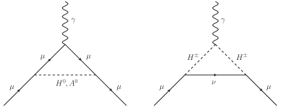
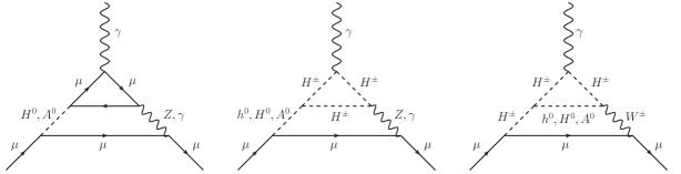
where we take the contributions at one- and two-loop level given in Ilisie:2015tra . The two-loop contributions come from the Barr-Zee diagrams (Barr:1990vd , see Fig. 19) with a fermion or boson loop which can give rise to significant contributions to $a_{\mu}^{\rm 2HDM}$. All Higgs bosons are present in these loops, therefore $a_{\mu}^{\rm 2HDM}$ depends not only on $\tan\beta$ and $m_{H^{+}}$, but also on $m_{A^{0}}$ and $m_{H^{0}}$, with a further dependence on the mixing angle $\alpha$.

Figure 20: Contour plots of the allowed 2HDM-II parameter space in the $(\tan\beta-m_{H^{+}})$ plane for $a_{\mu}$, using the Standard Model prediction by WP20 Aoyama:2020ynm (BMW Borsanyi:2020mff ) (left (right) plot), fixing the additional parameters as $\cos(\beta-\alpha)=0,\,m_{H^{0}}=m_{A^{0}}=m_{H^{+}}$. The lighter contour indicates the allowed parameter space at $2\sigma$ confidence level while the darker contour corresponds to $1\sigma$.

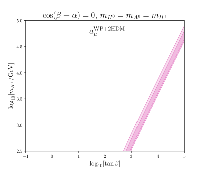
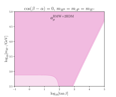
From Fig. 20 we find that the 2HDM-II cannot explain the discrepancy between the experimental number for the anomalous magnetic moment of the muon and the white paper prediction as the required values of $\tan\beta$ lie in the non-perturbative region. Obviously the BMW prediction yields a consistency of experiment and theory within 2$\sigma$ and thus a large portion of the 2HDM-II parameter space is still allowed.

7.3 Electroweak Phase Transition

The electroweak phase transition (EWPT) is a mechanism which can generate the baryon asymmetry we observe in the Universe today through the process of EW baryogenesis, with the requirement that the EWPT is of strong first order (SFO). In the SM this could be achieved for $m_{h^{0}}\lesssim 70\,$ GeV Kajantie:1996mn , however the measurement of the SM Higgs boson mass as $m_{h^{0}}=125.1\pm 0.14\,$ GeV Zyla:2020zbs means we now require BSM physics to achieve a SFOEWPT; a 2HDM is in principle capable of generating this. For recent work testing the 2HDM for a SFOEWPT across large regions in its parameter space, see e.g. Refs. Basler:2016obg ; Su:2020pjw ; Dorsch:2016nrg , in which the authors find regions where the 2HDM-II could support a SFOEWPT, however only for Higgs masses less than $1\,$TeV. In Wang:2021ayg , the strength of the EWPT in the 2HDM-II is tested for Higgs masses $\gtrsim 600\,$GeV; a FOEWPT can be found for these masses but it is not strong enough to support EW baryogenesis. Furthermore, a SFOEWPT appears to favour a mass splitting ($\sim 200\,$GeV Su:2020pjw ) between $H^{+}$ and $H^{0}$, and $m_{A^{0}}\sim m_{H^{+}}$ Su:2020pjw ; Dorsch:2016nrg . This could still be allowed by our results in Section 3, however only for low charged Higgs masses, in tension with the global fit of Fig. 16.

In this work, we use the BSMPT package Basler:2018cwe ; Basler:2020nrq to calculate the strength of the EWPT for selected parameter points across our fit. The BSMPT package calculates the strength of the EWPT for the 2HDM in the lambda parameter basis ($\lambda_{i}$, $m_{12}^{2}$, $\tan\beta$). We have so far primarily worked in the mass basis ($m_{A^{0}},m_{H^{0}},m_{h^{0}},m_{H^{+}},\tan\beta,\cos(\beta-\alpha)$), and so must convert to the lambda basis. In the alignment limit, a sufficient but not necessary condition for vacuum stability is Kling:2016opi

$$m_{12}^{2}=m_{H^{0}}^{2}\sin\beta\cos\beta\,\cap\,m_{h^{0}}^{2}+m_{H^{\pm}}^{2}-m_{H^{0}}^{2}>0\,\cap\,m_{h^{0}}^{2}+m_{A^{0}}^{2}-m_{H^{0}}^{2}>0.$$ (51)

We then use this, along with Eqs. (11)-(15), to perform the conversion, while making the assumption that $\cos(\beta-\alpha)$ is small, which is of course in line with our constraints. This is only appropriate when the conditions of Eq. (51) are fulfilled, i.e. primarily for $m_{H^{0}}\lesssim m_{A^{0}},m_{H^{+}}$.

The BSMPT package parameterises the strength of the EWPT in the 2HDM by calculating

$$\xi_{c}=\frac{\omega_{c}}{T_{c}},$$ (52)

where $\omega_{c}$ is the high-temperature VEV ($\omega_{c}^{2}=\omega_{1}^{2}(T_{c})+\omega_{2}^{2}(T_{c})$ and $\omega_{i}(T=0)=v_{i}$) at the critical temperature $T_{c}$. The BSMPT package only passes a result if $\xi_{c}>0$, with the desired SFOEWPT indicated by $\xi_{c}>1$.

$\tan\beta$	Mass Basis (GeV)			Lambda Basis			$m_{12}^{2}$	$\omega_{c}$	$T_{c}$	$\xi_{c}$
	$m_{H^{+}}$	$m_{H^{0}}$	$m_{A^{0}}$	$\lambda_{3}$	$\lambda_{4}$	$\lambda_{5}$	(GeV2)	(GeV)	(GeV)
$4.2$	$50000$	$50000$	$50000$	$0.26$	$0$	$0$	$5.6\times 10^{8}$	$0.66$	$162$	$0.004$
$4.2$	$2320$	$2320$	$2320$	$0.26$	$0$	$0$	$1.2\times 10^{6}$	$23$	$162$	$0.14$
$4.2$	$2320$	$2250$	$2280$	$10.8$	$-8.3$	$-2.2$	$1.1\times 10^{6}$	$31$	$186$	$0.17$
$1.0$	$2320$	$2320$	$2320$	$0.26$	$0$	$0$	$2.7\times 10^{6}$	$23$	$162$	$0.14$
$10$	$2320$	$2320$	$2320$	$0.26$	$0$	$0$	$5.3\times 10^{5}$	$24$	$162$	$0.15$
$4.2$	$860$	$710$	$860$	$8.03$	$-3.9$	$-3.9$	$1.1\times 10^{5}$	$142$	$175$	$0.81$
$4.2$	$860$	$690$	$860$	$8.95$	$-4.3$	$-4.3$	$1.1\times 10^{5}$	$177$	$176$	$1.00$
$4.2$	$680$	$470$	$680$	$8.22$	$-4.0$	$-4.0$	$5.0\times 10^{4}$	$211$	$149$	$1.42$
$4.2$	$570$	$320$	$570$	$7.60$	$-3.7$	$-3.7$	$2.3\times 10^{4}$	$226$	$126$	$1.79$
$4.2$	$490$	$250$	$490$	$6.12$	$-2.9$	$-2.9$	$1.4\times 10^{4}$	$207$	$126$	$1.64$
$4.2$	$490$	$490$	$490$	$0.26$	$0$	$0$	$5.4\times 10^{4}$	$24$	$161$	$0.15$

Table 3: Table of results for the EWPT in the 2HDM. We consider the exact alignment limit, $\cos(\beta-\alpha)=0$, and in addition we employ the condition by Eq. (51). In this limit, as follows from Eqs. (11)-(15), one gets: $\lambda_{1}=\lambda_{2}=m_{h^{0}}^{2}/v^{2}=0.26$, i.e. $\lambda_{1,2}$ are fixed and independent of the Higgs masses and $\tan\beta$ (and therefore not again shown in the table). In addition, one obtains that $\lambda_{3,4,5}$ are independent of $\tan\beta$, and $\lambda_{3}+\lambda_{4}+\lambda_{5}=m_{h^{0}}^{2}/v^{2}=0.26$. For similar discussions of the lambda basis, see e.g. BhupalDev:2014bir .

We choose $M=50\,$TeV as a benchmark for more extreme masses, the best-fit point of our degenerate mass fit, and lower limits in $m_{H^{+}}$ at $\sim 2,3,4,5\sigma$ where we select more favourable mass splittings as points to test for a SFOEWPT. We also show some variations in $\tan\beta$ at the best-fitting degenerate masses. In Table 3, we present our selected parameter points in both bases, and then also the results produced by the BSMPT package. As is generally favoured by our fits, for higher masses we mostly test parameter points in the limit of degenerate masses, since this will satisfy the conditions of Eq. (51) and the small mass splittings allowed at higher mass scales have only small effects, as is shown in one benchmark point. However for lower masses where these splittings are more significant, we consider further benchmark points allowing for mass splitting more favourable for a SFOEWPT Su:2020pjw , and find that demanding degeneracy for these lower masses is a poorer choice.

We find that for most of our allowed parameter space, a SFOEWPT is not possible due to the large mass scales involved. From the benchmark points at higher masses, we find a maximum of $\xi_{c}=0.17$; much smaller than required. For our benchmark points at lower masses however, the outlook improves, where we first find a $\xi_{c}\geq 1$ for a parameter point at $\sim 2\sigma$ from the global best fit point. On the other hand, we note that all points in Table 3 with a ratio $\xi_{c}\geq 1$ require some of the couplings $|\lambda_{i}|>4$, which could be in conflict with perturbativity, depending on what constraint we apply; see the beginning of Section 3.1. As we have only chosen a few benchmark points, we cannot rule out the possibility of a $\xi_{c}\geq 1$ at some point closer to our best fit, however this seems unlikely given the trends shown here and in other works. Therefore to accommodate a SFOEWPT in the 2HDM-II, we would require much lower Higgs masses than are favoured by the global fit. But for such regions of the parameter space the 2HDM-II will no longer perform better in the overall fit compared to the SM.

8 Conclusion

In this work we have investigated theoretical bounds on the 2HDM-II stemming from perturbativity, unitarity and vacuum stability as well as experimental constraints stemming from electroweak precision, Higgs signal strengths, flavour observables and the anomalous magnetic moment of the muon. All in all, we find that the 2HDM-II can accommodate the data better than the SM. The best fit point for the 2HDM-II lies around

$$m_{H^{+}}\approx m_{H^{0}} \approx m_{A^{0}}\approx 2\,\mbox{TeV}\,,$$ (53)

$$\tan\beta\approx 4, \quad\cos(\beta-\alpha)\approx 0.01\,.$$

For the charged Higgs mass we find a lower limit of 680 GeV at $3\sigma$ and the remaining Higgses have to be largely degenerate – this requirement becomes stronger the heavier the Higgs masses become. For low values of the charged Higgs mass, $\tan\beta$ is severely constrained to lie around a value of 4, while for high values of the charged Higgs mass (around 50 TeV) $\tan\beta$ should be in the region between 0.1 and 300. We further find that the wrong-sign limit is disfavoured by Higgs signal strengths and excluded by the global fit by more than $5\sigma$ and that only small deviations from the alignment limit are possible.

Experiments currently observe some deviations from SM predictions, in particular in $R(D^{(*)})$, $R_{K^{(*)}}$ and the anomalous magnetic moment of the muon. The tensions in $R(D^{(*)})$ will either be enhanced in the 2HDM-II or to be resolved, they would require parameter regions in the $(\tan\beta-m_{H^{+}})$ plane which are excluded by other flavour observables. Eliminating the tension in $R_{K^{(*)}}$ would require charged Higgs masses below 1 GeV and non-perturbative values of $\tan\beta$. The 2HDM-II can also not resolve the discrepancy between the measurement of the magnetic moment of the muon and the white paper prediction.

Finally we found that the allowed parameter space of the 2HDM-II strongly disfavours the existence of a sufficiently strong first order phase transition for EW baryogenesis. This requires mass splittings discouraged by theoretical constraints, and low masses of the charged Higgs – at least $2\sigma$ away from our best fit point, which makes this model theoretically much less attractive.

As a next step we plan to study more types of 2HDMs and also investigate implications of our findings for future collider searches.

Appendix A Inputs and Observables

Table 4: Table of the Higgs signal strengths used in the analysis in Section 5.

Observable	Experimental value	Source	SM prediction
Higgs signal strengths
$\mu^{\gamma\gamma}_{\text{ggF}}$	$1.03\pm 0.11$	ATLAS:2020qdt	1
	$1.09^{+0.15}_{-0.14}$	CMS:2020gsy
	$1.07^{+0.12}_{-0.11}$	Sirunyan:2021ybb
$\mu_{\text{ggF}}^{ZZ}$	$0.94^{+0.11}_{-0.10}$	ATLAS:2020qdt	1
	$0.98^{+0.12}_{-0.11}$	CMS:2020gsy
$\mu^{WW}_{\text{ggF}}$	$1.08^{+0.19}_{-0.18}$	ATLAS:2020qdt	1
	$1.28^{+0.20}_{-0.19}$	CMS:2020gsy
	$1.20^{+0.16}_{-0.15}$	ATLAS:2021upe
$\mu^{Z\gamma}_{\text{ggF}}$	$2.0^{+1.0}_{-0.9}$	Aad:2020plj	1
$\mu^{\tau\tau}_{\text{ggF}}$	$1.02^{+0.60}_{-0.55}$	ATLAS:2020qdt	1
	$0.39^{+0.38}_{-0.39}$	CMS:2020gsy
$\mu^{\mu\mu}_{\text{ggF}}$	$1.2\pm 0.6$	Aad:2020xfq	1
	$0.31^{+1.82}_{-1.81}$	CMS:2020gsy
	$1.19^{+0.42}_{-0.41}$	Sirunyan:2020two
$\mu^{bb}_{\text{ggF}}$	$2.51^{+2.43}_{-2.01}$	ATLAS:2020qdt	1
	$2.45^{+2.53}_{-2.35}$	CMS:2020gsy
$\mu^{\gamma\gamma}_{\text{VBF}}$	$1.31^{+0.26}_{-0.23}$	ATLAS:2020qdt	1
	$0.77^{+0.37}_{-0.29}$	CMS:2020gsy
	$1.04^{+0.34}_{-0.31}$	Sirunyan:2021ybb
$\mu^{ZZ}_{\text{VBF}}$	$1.25^{+0.50}_{-0.41}$	ATLAS:2020qdt	1
	$0.57^{+0.46}_{-0.36}$	CMS:2020gsy
$\mu^{WW}_{\text{VBF}}$	$0.60^{+0.36}_{-0.34}$	ATLAS:2020qdt	1
	$0.63^{+0.65}_{-0.61}$	CMS:2020gsy
	$0.99^{+0.24}_{-0.20}$	ATLAS:2021upe
$\mu^{\tau\tau}_{\text{VBF}}$	$1.15^{+0.57}_{-0.53}$	ATLAS:2020qdt	1
	$1.05^{+0.30}_{-0.29}$	CMS:2020gsy
$\mu^{\mu\mu}_{\text{VBF}}$	$3.18^{+8.22}_{-7.93}$	CMS:2020gsy	1
$\mu^{bb}_{\text{VBF}}$	$3.03^{+1.67}_{-1.62}$	ATLAS:2020qdt	1
	$0.95^{+0.38}_{-0.36}$	ATLAS:2020bhl
$\mu^{\gamma\gamma}_{\text{Wh}}$	$3.76^{+1.48}_{-1.35}$	Sirunyan:2018koj	1
$\mu^{WW}_{\text{Wh}}$	$2.85^{+2.11}_{-1.87}$	CMS:2020gsy	1
$\mu^{\tau\tau}_{\text{Wh}}$	$3.01^{+1.65}_{-1.51}$	CMS:2020gsy	1
$\mu^{bb}_{\text{Wh}}$	$1.27^{+0.42}_{-0.40}$	CMS:2020gsy	1
	$0.95^{+0.27}_{-0.25}$	Aad:2020jym
$\mu^{\gamma\gamma}_{\text{Zh}}$	$0.00\pm 1.14$	Sirunyan:2018koj	1
$\mu^{WW}_{\text{Zh}}$	$0.90^{+1.77}_{-1.43}$	CMS:2020gsy	1
$\mu^{\tau\tau}_{\text{Zh}}$	$1.53^{+1.60}_{-1.37}$	CMS:2020gsy	1
$\mu^{bb}_{\text{Zh}}$	$0.93^{+0.33}_{-0.31}$	CMS:2020gsy	1
	$1.08^{+0.25}_{-0.23}$	Aad:2020jym
$\mu^{cc}_{\text{Zh}}$	$37^{+20}_{-19}$	Sirunyan:2019qia	1
$\mu^{\gamma\gamma}_{\text{Vh}}$	$1.32^{+0.33}_{-0.30}$	ATLAS:2020qdt	1
	$1.34^{+0.36}_{-0.33}$	Sirunyan:2021ybb
$\mu^{ZZ}_{\text{Vh}}$	$1.53^{+1.13}_{-0.92}$	ATLAS:2020qdt	1
	$1.10^{+0.96}_{-0.74}$	CMS:2020gsy
$\mu^{bb}_{\text{Vh}}$	$1.02^{+0.18}_{-0.17}$	ATLAS:2020qdt	1
	$1.03^{+0.28}_{-0.17}$	Aad:2020jym
$\mu^{\gamma\gamma}_{\text{tth}}$	$0.90^{+0.41}_{-0.35}$	ATLAS:2020qdt	1
	$1.62^{+0.52}_{-0.43}$	CMS:2020gsy
	$1.35^{+0.34}_{-0.28}$	Sirunyan:2021ybb
$\mu^{ZZ}_{\text{tth}}$	$0.25^{+1.03}_{-0.25}$	CMS:2020gsy	1
$\mu^{WW}_{\text{tth}}$	$0.93^{+0.48}_{-0.45}$	CMS:2020gsy	1
$\mu^{VV}_{\text{tth}}$	$1.72^{+0.56}_{-0.53}$	ATLAS:2020qdt	1
$\mu^{\tau\tau}_{\text{tth}}$	$1.20^{+1.07}_{-0.93}$	ATLAS:2020qdt	1
	$0.81^{+0.74}_{-0.67}$	CMS:2020gsy
$\mu^{bb}_{\text{tth}}$	$0.79^{+0.60}_{-0.59}$	ATLAS:2020qdt	1
	$1.13^{+0.33}_{-0.30}$	CMS:2020gsy

Table 5: List of the Oblique parameters used in the analysis in Section 4.

Observable	Experimental value	Source	SM prediction
Oblique parameters
S	$0.02\pm 0.10$	Zyla:2020zbs	0
T	$0.07\pm 0.12$	Zyla:2020zbs	0
U	$0.00\pm 0.09$	Zyla:2020zbs	0

Table 6: Table of flavour observables (except $b\to s\ell^{+}\ell^{-}$) used in the analysis. The stated SM predictions are our calculations through flavio, where we have modified some appropriately in order to closely replicate the most recent averages or predictions, for example in $B$-mixing and $B\to X_{s}\gamma$ (marked by ${\color[rgb]{1,0,0}\definecolor[named]{pgfstrokecolor}{rgb}{1,0,0}*}$ in the fourth column).

Observable	Experimental value	Source	SM prediction
Tree-level leptonic decays
$\Gamma(\pi^{+}\to\mu^{+}\nu_{\mu})$	$(2.528\pm 0.005)\times 10^{-17}\,$eV	Zyla:2020zbs	$(2.521\pm 0.003)\times 10^{-17}\,$eV
${\cal B}(K^{+}\to\mu^{+}\nu_{\mu})$	$(63.56\pm 0.11)\times 10^{-2}$	Zyla:2020zbs	$(63.91\pm 0.93)\times 10^{-2}$
${\cal B}(B^{+}\to\mu^{+}\nu_{\mu})$	$(5.3\pm 2.2)\times 10^{-7}$	Zyla:2020zbs	$(4.15\pm 0.51)\times 10^{-7}$
${\cal B}(B^{+}\to\tau^{+}\nu_{\tau})$	$(1.09\pm 0.24)\times 10^{-4}$	Zyla:2020zbs	$(9.24\pm 1.13)\times 10^{-5}$
${\cal B}(D^{+}\to\mu^{+}\nu_{\mu})$	$(3.74\pm 0.17)\times 10^{-4}$	Zyla:2020zbs	$(3.97\pm 0.04)\times 10^{-4}$
${\cal B}(D^{+}\to\tau^{+}\nu_{\tau})$	$(1.20\pm 0.27)\times 10^{-3}$	Zyla:2020zbs	$(1.07\pm 0.01)\times 10^{-3}$
${\cal B}(D_{s}^{+}\to\mu^{+}\nu_{\mu})$	$(5.49\pm 0.16)\times 10^{-3}$	Zyla:2020zbs	$(5.31\pm 0.04)\times 10^{-3}$
${\cal B}(D_{s}^{+}\to\tau^{+}\nu_{\tau})$	$(5.48\pm 0.23)\times 10^{-2}$	Zyla:2020zbs	$(5.22\pm 0.04)\times 10^{-2}$
${\cal B}(\tau^{+}\to K^{+}\nu_{\tau})$	$(6.96\pm 0.10)\times 10^{-3}$	Zyla:2020zbs	$(7.07\pm 0.10)\times 10^{-3}$
${\cal B}(\tau^{+}\to\pi^{+}\nu_{\tau})$	$(10.82\pm 0.05)\times 10^{-2}$	Zyla:2020zbs	$(10.85\pm 0.13)\times 10^{-2}$
Tree-level semi-leptonic decays
${\cal B}(B^{0}\to D^{-}\ell^{+}\nu_{\ell})$	$(2.31\pm 0.10)\times 10^{-2}$	Amhis:2019ckw	$(2.26\pm 0.18)\times 10^{-2}$
${\cal B}(B^{+}\to D^{0}\ell^{+}\nu_{\ell})$	$(2.35\pm 0.10)\times 10^{-2}$	Amhis:2019ckw	$(2.45\pm 0.19)\times 10^{-2}$
${\cal B}(B^{0}\to D^{*-}\ell^{+}\nu_{\ell})$	$(5.06\pm 0.12)\times 10^{-2}$	Amhis:2019ckw	$(4.82\pm 0.44)\times 10^{-2}$
${\cal B}(B^{+}\to D^{*0}\ell^{+}\nu_{\ell})$	$(5.66\pm 0.22)\times 10^{-2}$	Amhis:2019ckw	$(5.20\pm 0.48)\times 10^{-2}$
${\cal B}(B^{+}\to\pi^{0}\ell^{+}\nu_{\ell})$	$(7.80\pm 0.27)\times 10^{-5}$	Zyla:2020zbs	$(6.37\pm 1.03)\times 10^{-5}$
${\cal B}(B^{0}\to\pi^{-}\ell^{+}\nu_{\ell})$	$(1.50\pm 0.06)\times 10^{-4}$	Zyla:2020zbs	$(1.18\pm 0.19)\times 10^{-4}$
${\cal B}(B^{+}\to\rho^{0}\ell^{+}\nu_{\ell})$	$(1.58\pm 0.11)\times 10^{-4}$	Zyla:2020zbs	$(2.19\pm 0.44)\times 10^{-4}$
${\cal B}(B^{0}\to\rho^{-}\ell^{+}\nu_{\ell})$	$(2.94\pm 0.21)\times 10^{-4}$	Zyla:2020zbs	$(4.06\pm 0.82)\times 10^{-4}$
${\cal B}(B^{0}_{s}\to D^{-}_{s}\mu^{+}\nu_{\mu})$	$(2.40\pm 0.12\pm 0.15\pm 0.06\pm 0.10)\times 10^{-2}$	Aaij:2020hsi ; Aaij:2021nyr	$(2.36\pm 0.18)\times 10^{-2}$ * McLean:2019qcx
${\cal B}(B^{0}_{s}\to D^{*-}_{s}\mu^{+}\nu_{\mu})$	$(5.19\pm 0.24\pm 0.47\pm 0.13\pm 0.14)\times 10^{-2}$	Aaij:2020hsi ; Aaij:2021nyr	$(4.99\pm 0.45)\times 10^{-2}$ * McLean:2019qcx
${\cal B}(D^{+}\to\bar{K}^{0}e^{+}\nu_{e})$	$(8.73\pm 0.10)\times 10^{-2}$	Zyla:2020zbs	$(9.08\pm 0.61)\times 10^{-2}$
${\cal B}(D^{+}\to\bar{K}^{0}\mu^{+}\nu_{\mu})$	$(8.76\pm 0.19)\times 10^{-2}$	Zyla:2020zbs	$(9.04\pm 0.61)\times 10^{-2}$
${\cal B}(D^{+}\to\pi^{0}e^{+}\nu_{e})$	$(3.72\pm 0.17)\times 10^{-3}$	Zyla:2020zbs	$(3.47\pm 0.20)\times 10^{-3}$
${\cal B}(D^{+}\to\pi^{0}\mu^{+}\nu_{\mu})$	$(3.50\pm 0.15)\times 10^{-3}$	Zyla:2020zbs	$(3.46\pm 0.19)\times 10^{-3}$
${\cal B}(D^{0}\to K^{-}e^{+}\nu_{e})$	$(3.542\pm 0.035)\times 10^{-2}$	Zyla:2020zbs	$(3.55\pm 0.24)\times 10^{-2}$
${\cal B}(D^{0}\to K^{-}\mu^{+}\nu_{\mu})$	$(3.41\pm 0.04)\times 10^{-2}$	Zyla:2020zbs	$(3.54\pm 0.24)\times 10^{-2}$
${\cal B}(D^{0}\to\pi^{-}e^{+}\nu_{e})$	$(2.91\pm 0.04)\times 10^{-3}$	Zyla:2020zbs	$(2.68\pm 0.15)\times 10^{-3}$
${\cal B}(D^{0}\to\pi^{-}\mu^{+}\nu_{\mu})$	$(2.67\pm 0.12)\times 10^{-3}$	Zyla:2020zbs	$(2.67\pm 0.15)\times 10^{-3}$
${\cal B}(K^{+}\to\pi^{0}e^{+}\nu_{e})$	$(5.07\pm 0.04)\times 10^{-2}$	Zyla:2020zbs	$(5.12\pm 0.06)\times 10^{-2}$
${\cal B}(K^{+}\to\pi^{0}\mu^{+}\nu_{\mu})$	$(3.352\pm 0.033)\times 10^{-2}$	Zyla:2020zbs	$(3.380\pm 0.043)\times 10^{-2}$
${\cal B}(K^{0}_{L}\to\pi^{+}e^{-}\bar{\nu}_{e})$	$(40.55\pm 0.11)\times 10^{-2}$	Zyla:2020zbs	$(40.82\pm 0.43)\times 10^{-2}$
${\cal B}(K^{0}_{L}\to\pi^{+}\mu^{-}\bar{\nu}_{\mu})$	$(27.04\pm 0.07)\times 10^{-2}$	Zyla:2020zbs	$(27.04\pm 0.30)\times 10^{-2}$
${\cal B}(K^{0}_{S}\to\pi^{+}e^{-}\bar{\nu}_{e})$	$(7.04\pm 0.08)\times 10^{-4}$	Zyla:2020zbs	$(7.15\pm 0.07)\times 10^{-4}$
${\cal B}(K^{0}_{S}\to\pi^{+}\mu^{-}\bar{\nu}_{\mu})$	$(4.69\pm 0.05)\times 10^{-4}$	Zyla:2020zbs	$(4.73\pm 0.05)\times 10^{-4}$
Tree-level LFU Ratios
$\mathcal{R}(D)$	$(0.340\pm 0.030)$	Amhis:2019ckw	$(0.303\pm 0.006)$
$\mathcal{R}(D^{*})$	$(0.295\pm 0.014)$	Amhis:2019ckw	$(0.255\pm 0.003)$
Radiative decays
${\cal B}(\bar{B}\to X_{s}\gamma)$	$(3.32\pm 0.15)\times 10^{-4}$	Amhis:2019ckw	$(3.40\pm 0.17)\times 10^{-4}$ ${\color[rgb]{1,0,0}\definecolor[named]{pgfstrokecolor}{rgb}{1,0,0}*}$ Misiak:2020vlo
FCNC leptonic decays
${\cal B}(B_{d}\to\mu^{+}\mu^{-})$	$(0.56\pm 0.70)\times 10^{-10}$	Altmannshofer:2021qrr	$(1.08\pm 0.13)\times 10^{-10}$
${\cal B}(B_{s}\to\mu^{+}\mu^{-})$	$(2.93\pm 0.35)\times 10^{-9}$	Altmannshofer:2021qrr	$(3.48\pm 0.26)\times 10^{-9}$
$B$-Mixing
$\Delta m_{d}$	$(0.5065\pm 0.0019)\,$ps-1	Amhis:2019ckw	$(0.533^{+0.022}_{-0.036})\,$ps-1 * DiLuzio:2019jyq
$\Delta m_{s}$	$(17.757\pm 0.021)\,$ps-1	Amhis:2019ckw	$(18.4^{+0.7}_{-1.2})\,$ps-1 * DiLuzio:2019jyq
Anomalous magnetic moments
$a_{\mu}$	$116592091(54)(33)\times 10^{-11}$	Zyla:2020zbs	$116591810(43)\times 10^{-11}$ * Aoyama:2020ynm
			$116591954(55)\times 10^{-11}$ * Borsanyi:2020mff

Table 7: Table of $b\to s\ell^{+}\ell^{-}$ observables (except $R_{K^{(*)}}$) used in the analysis. We include correlations between measurements when provided by the sources. The stated SM predictions are our calculations through flavio. The modes marked by * assume averaging of $B^{+}$ and $B^{0}$ decays.

Mode	Observable	Source	Bin	Experimental value	SM prediction
$B^{+}\to K^{+}\mu^{+}\mu^{-}$	$10^{\,8}\,{\rm GeV}^{2}\times\frac{\Delta\cal B}{\Delta q^{2}}$	LHCb Aaij:2014pli	$[0.1,0.98]$	$3.32\pm 0.18\pm 0.17$	$3.34\pm 0.63$
			$[1.1,2]$	$2.33\pm 0.15\pm 0.12$	$3.33\pm 0.63$
			$[2,3]$	$2.82\pm 0.16\pm 0.14$	$3.32\pm 0.62$
			$[3,4]$	$2.54\pm 0.15\pm 0.13$	$3.30\pm 0.62$
			$[4,5]$	$2.21\pm 0.14\pm 0.11$	$3.28\pm 0.62$
			$[5,6]$	$2.31\pm 0.14\pm 0.12$	$3.26\pm 0.61$
			$[15,16]$	$1.61\pm 0.10\pm 0.08$	$2.25\pm 0.33$
			$[16,17]$	$1.64\pm 0.10\pm 0.08$	$2.03\pm 0.28$
			$[17,18]$	$2.06\pm 0.11\pm 0.10$	$1.77\pm 0.23$
			$[18,19]$	$1.37\pm 0.10\pm 0.07$	$1.49\pm 0.19$
			$[19,20]$	$0.74\pm 0.08\pm 0.04$	$1.17\pm 0.14$
			$[20,21]$	$0.59\pm 0.07\pm 0.03$	$0.82\pm 0.10$
			$[21,22]$	$0.43\pm 0.07\pm 0.02$	$0.44\pm 0.05$
$B^{0}\to K^{0}\mu^{+}\mu^{-}$	$10^{\,8}\,{\rm GeV}^{2}\times\frac{\Delta\cal B}{\Delta q^{2}}$	LHCb Aaij:2014pli	$[0.1,2]$	$1.22^{+0.59}_{-0.52}\pm 0.06$	$3.10\pm 0.58$
			$[2,4]$	$1.87^{+0.55}_{-0.49}\pm 0.09$	$3.07\pm 0.58$
			$[4,6]$	$1.73^{+0.53}_{-0.48}\pm 0.09$	$3.03\pm 0.57$
			$[15,17]$	$1.43^{+0.35}_{-0.32}\pm 0.07$	$1.98\pm 0.28$
			$[17,19]$	$0.78^{+0.17}_{-0.15}\pm 0.04$	$1.50\pm 0.19$
$B^{+}\to K^{*+}\mu^{+}\mu^{-}$	$10^{\,8}\,{\rm GeV}^{2}\times\frac{\Delta\cal B}{\Delta q^{2}}$	LHCb Aaij:2014pli	$[0.1,2]$	$5.92^{+1.44}_{-1.30}\pm 0.40$	$7.53\pm 1.11$
			$[2,4]$	$5.59^{+1.59}_{-1.44}\pm 0.38$	$4.60\pm 0.63$
			$[4,6]$	$2.49^{+1.10}_{-0.96}\pm 0.17$	$5.13\pm 0.74$
			$[15,17]$	$6.44^{+1.29}_{-1.15}\pm 0.44$	$7.19\pm 0.89$
			$[17,19]$	$1.16^{+0.91}_{-0.76}\pm 0.08$	$4.96\pm 0.68$
$B^{+}\to K^{*+}\mu^{+}\mu^{-}$	$F_{L}$	LHCb Aaij:2020ruw	$[0.1,0.98]$	$0.34^{+0.10}_{-0.10}\pm 0.06$	$0.303\pm 0.052$
			$[1.1,2.5]$	$0.54^{+0.18}_{-0.19}\pm 0.03$	$0.767\pm 0.043$
			$[2.5,4]$	$0.17^{+0.24}_{-0.14}\pm 0.04$	$0.798\pm 0.035$
			$[4,6]$	$0.67^{+0.11}_{-0.14}\pm 0.03$	$0.712\pm 0.048$
			$[15,17]$	$0.41^{+0.18}_{-0.14}\pm 0.02$	$0.346\pm 0.022$
			$[17,19]$	$0.34^{+0.11}_{-0.12}\pm 0.04$	$0.326\pm 0.016$
$B^{+}\to K^{*+}\mu^{+}\mu^{-}$	$P_{1}$	LHCb Aaij:2020ruw	$[0.1,0.98]$	$\phantom{-}0.44^{+0.38}_{-0.40}\pm 0.11$	$\phantom{-}0.045\pm 0.027$
			$[1.1,2.5]$	$\phantom{-}1.60^{+4.92}_{-1.75}\pm 0.32$	$\phantom{-}0.022\pm 0.047$
			$[2.5,4]$	$-0.29^{+1.43}_{-1.04}\pm 0.22$	$-0.116\pm 0.036$
			$[4,6]$	$-1.24^{+0.99}_{-1.17}\pm 0.29$	$-0.176\pm 0.046$
			$[15,17]$	$-0.88^{+0.41}_{-0.67}\pm 0.07$	$-0.531\pm 0.050$
			$[17,19]$	$-0.40^{+0.58}_{-0.57}\pm 0.09$	$-0.746\pm 0.036$
$B^{+}\to K^{*+}\mu^{+}\mu^{-}$	$P_{2}$	LHCb Aaij:2020ruw	$[0.1,0.98]$	$-0.05^{+0.12}_{-0.12}\pm 0.03$	$-0.136\pm 0.008$
			$[1.1,2.5]$	$-0.28^{+0.24}_{-0.42}\pm 0.15$	$-0.451\pm 0.017$
			$[2.5,4]$	$\phantom{-}0.03^{+0.26}_{-0.25}\pm 0.11$	$-0.054\pm 0.114$
			$[4,6]$	$-0.15^{+0.19}_{-0.20}\pm 0.06$	$\phantom{-}0.294\pm 0.081$
			$[15,17]$	$\phantom{-}0.45^{+0.03}_{-0.07}\pm 0.03$	$\phantom{-}0.414\pm 0.016$
			$[17,19]$	$\phantom{-}0.14^{+0.10}_{-0.10}\pm 0.04$	$\phantom{-}0.320\pm 0.020$
$B^{+}\to K^{*+}\mu^{+}\mu^{-}$	$P_{3}$	LHCb Aaij:2020ruw	$[0.1,0.98]$	$-0.42^{+0.20}_{-0.21}\pm 0.05$	$\phantom{-}0.0015\pm 0.0134$
			$[1.1,2.5]$	$-0.09^{+0.70}_{-0.99}\pm 0.18$	$\phantom{-}0.0040\pm 0.0242$
			$[2.5,4]$	$-0.45^{+0.50}_{-0.62}\pm 0.20$	$\phantom{-}0.0039\pm 0.0103$
			$[4,6]$	$\phantom{-}0.52^{+0.82}_{-0.62}\pm 0.15$	$\phantom{-}0.0025\pm 0.0154$
			$[15,17]$	$-0.23^{+0.16}_{-0.20}\pm 0.02$	$-0.0004\pm 0.0003$
			$[17,19]$	$\phantom{-}0.12^{+0.21}_{-0.21}\pm 0.02$	$-0.0003\pm 0.0002$
$B^{+}\to K^{*+}\mu^{+}\mu^{-}$	$P_{4}^{\prime}$	LHCb Aaij:2020ruw	$[0.1,0.98]$	$-0.09^{+0.36}_{-0.35}\pm 0.12$	$\phantom{-}0.234\pm 0.012$
			$[1.1,2.5]$	$\phantom{-}0.58^{+0.62}_{-0.56}\pm 0.11$	$-0.066\pm 0.047$
			$[2.5,4]$	$-0.81^{+1.09}_{-0.84}\pm 0.14$	$-0.392\pm 0.048$
			$[4,6]$	$-0.79^{+0.47}_{-0.28}\pm 0.09$	$-0.502\pm 0.028$
			$[15,17]$	$-0.32^{+0.23}_{-0.22}\pm 0.08$	$-0.618\pm 0.010$
			$[17,19]$	$-0.57^{+0.29}_{-0.36}\pm 0.13$	$-0.660\pm 0.007$
$B^{+}\to K^{*+}\mu^{+}\mu^{-}$	$P_{5}^{\prime}$	LHCb Aaij:2020ruw	$[0.1,0.98]$	$\phantom{-}0.51^{+0.30}_{-0.28}\pm 0.12$	$\phantom{-}0.684\pm 0.024$
			$[1.1,2.5]$	$\phantom{-}0.88^{+0.70}_{-0.71}\pm 0.10$	$\phantom{-}0.112\pm 0.083$
			$[2.5,4]$	$-0.87^{+1.00}_{-1.68}\pm 0.09$	$-0.517\pm 0.107$
			$[4,6]$	$-0.25^{+0.32}_{-0.40}\pm 0.09$	$-0.763\pm 0.077$
			$[15,17]$	$-0.14^{+0.21}_{-0.20}\pm 0.06$	$-0.673\pm 0.036$
			$[17,19]$	$-0.66^{+0.36}_{-0.80}\pm 0.13$	$-0.487\pm 0.035$
$B^{+}\to K^{*+}\mu^{+}\mu^{-}$	$P_{6}^{\prime}$	LHCb Aaij:2020ruw	$[0.1,0.98]$	$-0.02^{+0.40}_{-0.34}\pm 0.06$	$-0.0476\pm 0.0376$
			$[1.1,2.5]$	$\phantom{-}0.25^{+1.22}_{-1.32}\pm 0.08$	$-0.0539\pm 0.0784$
			$[2.5,4]$	$-0.37^{+1.59}_{-3.91}\pm 0.05$	$-0.0439\pm 0.1071$
			$[4,6]$	$-0.09^{+0.40}_{-0.41}\pm 0.05$	$-0.0285\pm 0.1159$
			$[15,17]$	$-0.48^{+0.21}_{-0.21}\pm 0.02$	$-0.0029\pm 0.0015$
			$[17,19]$	$\phantom{-}0.12^{+0.33}_{-0.33}\pm 0.04$	$-0.0012\pm 0.0007$
$B^{+}\to K^{*+}\mu^{+}\mu^{-}$	$P_{8}^{\prime}$	LHCb Aaij:2020ruw	$[0.1,0.98]$	$\phantom{-}0.45^{+0.50}_{-0.39}\pm 0.09$	$-0.0326\pm 0.0225$
			$[1.1,2.5]$	$\phantom{-}0.12^{+0.75}_{-0.76}\pm 0.05$	$-0.0271\pm 0.0354$
			$[2.5,4]$	$\phantom{-}0.12^{+7.89}_{-4.95}\pm 0.07$	$-0.0182\pm 0.0394$
			$[4,6]$	$-0.15^{+0.44}_{-0.48}\pm 0.05$	$-0.0114\pm 0.0377$
			$[15,17]$	$-0.34^{+0.23}_{-0.22}\pm 0.04$	$\phantom{-}0.0007\pm 0.0006$
			$[17,19]$	$\phantom{-}0.36^{+0.37}_{-0.33}\pm 0.07$	$\phantom{-}0.0003\pm 0.0002$
$B^{0}\to K^{*0}\mu^{+}\mu^{-}$	$F_{L}$	LHCb Aaij:2020nrf	$[0.1,0.98]$	$0.255\pm 0.032\pm 0.007$	$0.295\pm 0.050$
			$[1.1,2.5]$	$0.655\pm 0.046\pm 0.017$	$0.760\pm 0.044$
			$[2.5,4]$	$0.756\pm 0.047\pm 0.023$	$0.796\pm 0.036$
			$[4,6]$	$0.684\pm 0.035\pm 0.015$	$0.711\pm 0.048$
			$[15,17]$	$0.352\pm 0.026\pm 0.009$	$0.348\pm 0.022$
			$[17,19]$	$0.344\pm 0.032\pm 0.025$	$0.328\pm 0.016$
$B^{0}\to K^{*0}\mu^{+}\mu^{-}$	$P_{1}$	LHCb Aaij:2020nrf	$[0.1,0.98]$	$\phantom{-}0.090\pm 0.119\pm 0.009$	$\phantom{-}0.0441\pm 0.0465$
			$[1.1,2.5]$	$-0.617\pm 0.296\pm 0.023$	$\phantom{-}0.0234\pm 0.0463$
			$[2.5,4]$	$\phantom{-}0.168\pm 0.371\pm 0.043$	$-0.116\pm 0.037$
			$[4,6]$	$\phantom{-}0.088\pm 0.235\pm 0.029$	$-0.178\pm 0.047$
			$[15,17]$	$-0.511\pm 0.096\pm 0.020$	$-0.534\pm 0.050$
			$[17,19]$	$-0.763\pm 0.152\pm 0.094$	$-0.751\pm 0.035$
$B^{0}\to K^{*0}\mu^{+}\mu^{-}$	$P_{2}$	LHCb Aaij:2020nrf	$[0.1,0.98]$	$-0.003\pm 0.038\pm 0.003$	$-0.132\pm 0.008$
			$[1.1,2.5]$	$-0.443\pm 0.100\pm 0.027$	$-0.451\pm 0.014$
			$[2.5,4]$	$-0.191\pm 0.116\pm 0.043$	$-0.063\pm 0.113$
			$[4,6]$	$\phantom{-}0.105\pm 0.068\pm 0.009$	$\phantom{-}0.292\pm 0.081$
			$[15,17]$	$\phantom{-}0.396\pm 0.022\pm 0.004$	$\phantom{-}0.413\pm 0.016$
			$[17,19]$	$\phantom{-}0.328\pm 0.032\pm 0.017$	$\phantom{-}0.317\pm 0.020$
$B^{0}\to K^{*0}\mu^{+}\mu^{-}$	$P_{3}$	LHCb Aaij:2020nrf	$[0.1,0.98]$	$\phantom{-}0.073\pm 0.057\pm 0.003$	$\phantom{-}0.0014\pm 0.0135$
			$[1.1,2.5]$	$\phantom{-}0.324\pm 0.147\pm 0.014$	$\phantom{-}0.0039\pm 0.0245$
			$[2.5,4]$	$\phantom{-}0.049\pm 0.195\pm 0.014$	$\phantom{-}0.0040\pm 0.0104$
			$[4,6]$	$-0.090\pm 0.139\pm 0.006$	$\phantom{-}0.0026\pm 0.0155$
			$[15,17]$	$-0.000\pm 0.056\pm 0.003$	$-0.0004\pm 0.0003$
			$[17,19]$	$\phantom{-}0.085\pm 0.068\pm 0.004$	$-0.0003\pm 0.0002$
$B^{0}\to K^{*0}\mu^{+}\mu^{-}$	$P_{4}^{\prime}$	LHCb Aaij:2020nrf	$[0.1,0.98]$	$\phantom{-}0.135\pm 0.118\pm 0.010$	$\phantom{-}0.251\pm 0.017$
			$[1.1,2.5]$	$-0.080\pm 0.142\pm 0.019$	$-0.064\pm 0.045$
			$[2.5,4]$	$-0.435\pm 0.169\pm 0.035$	$-0.393\pm 0.046$
			$[4,6]$	$-0.312\pm 0.115\pm 0.013$	$-0.504\pm 0.028$
			$[15,17]$	$-0.626\pm 0.069\pm 0.018$	$-0.619\pm 0.010$
			$[17,19]$	$-0.647\pm 0.086\pm 0.057$	$-0.661\pm 0.007$
$B^{0}\to K^{*0}\mu^{+}\mu^{-}$	$P_{5}^{\prime}$	LHCb Aaij:2020nrf	$[0.1,0.98]$	$\phantom{-}0.521\pm 0.095\pm 0.024$	$\phantom{-}0.688\pm 0.024$
			$[1.1,2.5]$	$\phantom{-}0.365\pm 0.122\pm 0.013$	$\phantom{-}0.140\pm 0.081$
			$[2.5,4]$	$-0.150\pm 0.144\pm 0.032$	$-0.500\pm 0.102$
			$[4,6]$	$-0.439\pm 0.111\pm 0.036$	$-0.757\pm 0.079$
			$[15,17]$	$-0.714\pm 0.074\pm 0.021$	$-0.670\pm 0.036$
			$[17,19]$	$-0.590\pm 0.084\pm 0.059$	$-0.483\pm 0.035$
$B^{0}\to K^{*0}\mu^{+}\mu^{-}$	$P_{6}^{\prime}$	LHCb Aaij:2020nrf	$[0.1,0.98]$	$\phantom{-}0.015\pm 0.094\pm 0.007$	$-0.055\pm 0.036$
			$[1.1,2.5]$	$-0.226\pm 0.128\pm 0.005$	$-0.070\pm 0.077$
			$[2.5,4]$	$-0.155\pm 0.148\pm 0.024$	$-0.052\pm 0.105$
			$[4,6]$	$-0.293\pm 0.117\pm 0.004$	$-0.030\pm 0.117$
			$[15,17]$	$\phantom{-}0.061\pm 0.085\pm 0.003$	$-0.003\pm 0.002$
			$[17,19]$	$\phantom{-}0.103\pm 0.105\pm 0.016$	$-0.001\pm 0.001$
$B^{0}\to K^{*0}\mu^{+}\mu^{-}$	$P_{8}^{\prime}$	LHCb Aaij:2020nrf	$[0.1,0.98]$	$-0.007\pm 0.122\pm 0.002$	$-0.0056\pm 0.0222$
			$[1.1,2.5]$	$-0.366\pm 0.158\pm 0.005$	$-0.0177\pm 0.0350$
			$[2.5,4]$	$\phantom{-}0.037\pm 0.169\pm 0.007$	$-0.0173\pm 0.0370$
			$[4,6]$	$\phantom{-}0.166\pm 0.127\pm 0.004$	$-0.0115\pm 0.0376$
			$[15,17]$	$\phantom{-}0.007\pm 0.086\pm 0.002$	$\phantom{-}0.0007\pm 0.0006$
			$[17,19]$	$-0.055\pm 0.099\pm 0.006$	$\phantom{-}0.0003\pm 0.0002$
$B^{0}\to K^{*0}\mu^{+}\mu^{-}$	$F_{L}$	ATLAS Aaboud:2018krd	$[0.04,2.0]$	$0.44\pm 0.08\pm 0.07$	$0.388\pm 0.057$
			$[2,4]$	$0.64\pm 0.11\pm 0.05$	$0.799\pm 0.035$
			$[4,6]$	$0.42\pm 0.13\pm 0.12$	$0.711\pm 0.048$
$B^{0}\to K^{*0}\mu^{+}\mu^{-}$	$P_{1}$	ATLAS Aaboud:2018krd	$[0.04,2.0]$	$-0.05\pm 0.30\pm 0.08$	$\phantom{-}0.0435\pm 0.0280$
			$[2,4]$	$-0.78\pm 0.51\pm 0.34$	$-0.095\pm 0.038$
			$[4,6]$	$\phantom{-}0.14\pm 0.43\pm 0.26$	$-0.178\pm 0.047$
$B^{0}\to K^{*0}\mu^{+}\mu^{-}$	$P_{4}^{\prime}$	ATLAS Aaboud:2018krd	$[0.04,2.0]$	$\phantom{-}0.31\pm 0.40\pm 0.20$	$\phantom{-}0.150\pm 0.018$
			$[2,4]$	$-0.76\pm 0.31\pm 0.21$	$-0.349\pm 0.050$
			$[4,6]$	$\phantom{-}0.64\pm 0.33\pm 0.18$	$-0.504\pm 0.028$
$B^{0}\to K^{*0}\mu^{+}\mu^{-}$	$P_{5}^{\prime}$	ATLAS Aaboud:2018krd	$[0.04,2.0]$	$\phantom{-}0.67\pm 0.26\pm 0.16$	$\phantom{-}0.513\pm 0.033$
			$[2,4]$	$-0.33\pm 0.31\pm 0.13$	$-0.409\pm 0.110$
			$[4,6]$	$\phantom{-}0.26\pm 0.35\pm 0.18$	$-0.757\pm 0.079$
$B^{0}\to K^{*0}\mu^{+}\mu^{-}$	$P_{6}^{\prime}$	ATLAS Aaboud:2018krd	$[0.04,2.0]$	$-0.18\pm 0.21\pm 0.04$	$-0.056\pm 0.042$
			$[2,4]$	$\phantom{-}0.31\pm 0.28\pm 0.19$	$-0.056\pm 0.042$
			$[4,6]$	$\phantom{-}0.06\pm 0.27\pm 0.13$	$-0.030\pm 0.117$
$B^{0}\to K^{*0}\mu^{+}\mu^{-}$	$P_{8}^{\prime}$	ATLAS Aaboud:2018krd	$[0.04,2.0]$	$-0.29\pm 0.48\pm 0.18$	$-0.0084\pm 0.0233$
			$[2,4]$	$\phantom{-}1.07\pm 0.41\pm 0.39$	$-0.0179\pm 0.0388$
			$[4,6]$	$-0.24\pm 0.42\pm 0.09$	$-0.0115\pm 0.0376$
$B^{0}\to K^{*0}\mu^{+}\mu^{-}$	$10^{\,8}\,{\rm GeV}^{2}\times\frac{\Delta\cal B}{\Delta q^{2}}$	CMS Khachatryan:2015isa	$[1,2]$	$4.6\pm 0.7\pm 0.3$	$4.59\pm 0.61$
			$[2,4.3]$	$3.3\pm 0.5\pm 0.2$	$4.25\pm 0.59$
			$[4.3,6]$	$3.4\pm 0.5\pm 0.3$	$4.79\pm 0.71$
			$[14.18,16]$	$6.7\pm 0.6\pm 0.5$	$7.06\pm 0.85$
			$[16,19]$	$4.2\pm 0.3\pm 0.3$	$5.16\pm 0.68$
$B^{0}\to K^{*0}\mu^{+}\mu^{-}$	$F_{L}$	CMS Khachatryan:2015isa	$[1,2]$	$0.64^{+0.10}_{-0.09}\pm 0.07$	$0.724\pm 0.050$
			$[2,4.3]$	$0.80^{+0.08}_{-0.08}\pm 0.06$	$0.793\pm 0.036$
			$[4.3,6]$	$0.62^{+0.10}_{-0.09}\pm 0.07$	$0.703\pm 0.049$
			$[14.18,16]$	$0.48^{+0.05}_{-0.06}\pm 0.04$	$0.362\pm 0.027$
			$[16,19]$	$0.38^{+0.05}_{-0.06}\pm 0.04$	$0.333\pm 0.020$
$B^{0}\to K^{*0}\mu^{+}\mu^{-}$	$A_{\rm FB}$	CMS Khachatryan:2015isa	$[1,2]$	$-0.27^{+0.17}_{-0.40}\pm 0.07$	$-0.156\pm 0.031$
			$[2,4.3]$	$-0.12^{+0.15}_{-0.17}\pm 0.05$	$-0.026\pm 0.033$
			$[4.3,6]$	$\phantom{-}0.01^{+0.15}_{-0.15}\pm 0.03$	$\phantom{-}0.132\pm 0.045$
			$[14.18,16]$	$\phantom{-}0.39^{+0.04}_{-0.06}\pm 0.01$	$\phantom{-}0.412\pm 0.018$
			$[16,19]$	$\phantom{-}0.35^{+0.07}_{-0.07}\pm 0.01$	$\phantom{-}0.349\pm 0.021$
$B^{0}\to K^{*0}\mu^{+}\mu^{-}$	$P_{1}$	CMS Sirunyan:2017dhj	$[1,2]$	$-0.12^{+0.46}_{-0.47}\pm 0.10$	$\phantom{-}0.044\pm 0.047$
			$[2,4.3]$	$-0.69^{+0.58}_{-0.27}\pm 0.23$	$-0.106\pm 0.038$
			$[4.3,6]$	$\phantom{-}0.53^{+0.24}_{-0.33}\pm 0.19$	$-0.180\pm 0.049$
			$[14.18,16]$	$-0.33^{+0.24}_{-0.23}\pm 0.20$	$-0.465\pm 0.051$
			$[16,19]$	$-0.53^{+0.19}_{-0.19}\pm 0.16$	$-0.680\pm 0.041$
$B^{0}\to K^{*0}\mu^{+}\mu^{-}$	$P_{5}^{\prime}$	CMS Sirunyan:2017dhj	$[1,2]$	$\phantom{-}0.10^{+0.32}_{-0.31}\pm 0.07$	$\phantom{-}0.289\pm 0.063$
			$[2,4.3]$	$-0.57^{+0.34}_{-0.31}\pm 0.18$	$-0.449\pm 0.104$
			$[4.3,6]$	$-0.96^{+0.22}_{-0.21}\pm 0.25$	$-0.769\pm 0.073$
			$[14.18,16]$	$-0.66^{+0.13}_{-0.20}\pm 0.18$	$-0.719\pm 0.035$
			$[16,19]$	$-0.56^{+0.12}_{-0.12}\pm 0.07$	$-0.547\pm 0.036$
$B^{+}\to K^{+}\mu^{+}\mu^{-}$	$10^{\,8}\,{\rm GeV}^{2}\times\frac{\Delta\cal B}{\Delta q^{2}}$	Belle Abdesselam:2019lab	$[0.1,4]$	$4.51^{+1.05}_{-0.94}\pm 0.20$	$3.33\pm 0.60$
			$[4,8.12]$	$3.00^{+0.68}_{-0.61}\pm 0.07$	$3.24\pm 0.61$
			$[1,6]$	$4.60^{+0.82}_{-0.76}\pm 0.10$	$3.30\pm 0.60$
$B^{+}\to K^{*+}\mu^{+}\mu^{-}$	$10^{\,8}\,{\rm GeV}^{2}\times\frac{\Delta\cal B}{\Delta q^{2}}$	Belle Abdesselam:2019wac	$[1.1,6]$	$2.45^{+1.84}_{-1.43}\pm 0.41$	$4.87\pm 0.77$
			$[15,19]$	$7.25^{+2.50}_{-2.00}\pm 0.75$	$6.08\pm 0.73$
$B^{0}\to K^{*0}\mu^{+}\mu^{-}$	$10^{\,8}\,{\rm GeV}^{2}\times\frac{\Delta\cal B}{\Delta q^{2}}$	Belle Abdesselam:2019wac	$[1.1,6]$	$3.88^{+1.22}_{-1.02}\pm 0.61$	$4.48\pm 0.71$
			$[15,19]$	$5.50^{+1.25}_{-1.00}\pm 0.50$	$5.60\pm 0.67$
$B_{s}^{0}\to\phi^{0}\mu^{+}\mu^{-}$	$10^{\,8}\,{\rm GeV}^{2}\times\frac{\Delta\cal B}{\Delta q^{2}}$	LHCb Aaij:2015esa ; Aaij:2021nyr	$[0.1,2]$	$5.54^{+0.69}_{-0.65}\pm 0.13\pm 0.27$	$7.92\pm 0.98$
			$[2,5]$	$2.42^{+0.40}_{-0.38}\pm 0.06\pm 0.12$	$4.94\pm 0.69$
			$[15,17]$	$4.28^{+0.54}_{-0.51}\pm 0.11\pm 0.21$	$6.60\pm 0.65$
			$[17,19]$	$3.75^{+0.54}_{-0.51}\pm 0.13\pm 0.18$	$3.93\pm 0.41$
$B_{s}^{0}\to\phi^{0}\mu^{+}\mu^{-}$	$F_{L}$	LHCb Aaij:2015esa	$[0.1,2]$	$0.20^{+0.08}_{-0.09}\pm 0.02$	$0.496\pm 0.037$
			$[2,5]$	$0.68^{+0.16}_{-0.13}\pm 0.03$	$0.811\pm 0.017$
			$[15,17]$	$0.23^{+0.09}_{-0.08}\pm 0.02$	$0.349\pm 0.015$
			$[17,19]$	$0.40^{+0.13}_{-0.15}\pm 0.02$	$0.328\pm 0.014$
$B_{s}^{0}\to\phi^{0}\mu^{+}\mu^{-}$	$S_{3}$	LHCb Aaij:2015esa	$[0.1,2]$	$-0.05^{+0.13}_{-0.13}\pm 0.01$	$\phantom{-}0.020\pm 0.006$
			$[2,5]$	$-0.06^{+0.19}_{-0.23}\pm 0.01$	$-0.009\pm 0.004$
			$[15,17]$	$-0.06^{+0.16}_{-0.19}\pm 0.01$	$-0.180\pm 0.007$
			$[17,19]$	$-0.07^{+0.23}_{-0.27}\pm 0.02$	$-0.262\pm 0.006$
$B_{s}^{0}\to\phi^{0}\mu^{+}\mu^{-}$	$S_{4}$	LHCb Aaij:2015esa	$[0.1,2]$	$\phantom{-}0.27^{+0.28}_{-0.18}\pm 0.01$	$\phantom{-}0.060\pm 0.007$
			$[2,5]$	$-0.47^{+0.30}_{-0.44}\pm 0.01$	$-0.148\pm 0.017$
			$[15,17]$	$-0.03^{+0.15}_{-0.15}\pm 0.01$	$-0.296\pm 0.004$
			$[17,19]$	$-0.39^{+0.25}_{-0.34}\pm 0.02$	$-0.313\pm 0.004$
$B_{s}^{0}\to\phi^{0}\mu^{+}\mu^{-}$	$S_{7}$	LHCb Aaij:2015esa	$[0.1,2]$	$\phantom{-}0.04^{+0.12}_{-0.12}\pm 0.00$	$-0.025\pm 0.018$
			$[2,5]$	$-0.03^{+0.18}_{-0.23}\pm 0.01$	$-0.020\pm 0.038$
			$[15,17]$	$\phantom{-}0.12^{+0.16}_{-0.15}\pm 0.01$	$-0.0013\pm 0.0006$
			$[17,19]$	$\phantom{-}0.20^{+0.29}_{-0.22}\pm 0.01$	$-0.0005\pm 0.0003$
$B\to X_{s}\,\mu^{+}\mu^{-}$ $\!\!\phantom{B}{}^{\color[rgb]{1,0,0}\definecolor[named]{pgfstrokecolor}{rgb}{1,0,0}*}$	$10^{6}\times\Delta{\cal B}$	BaBar Lees:2013nxa	$[1,6]$	$0.66^{+0.87}_{-0.80}\pm 0.07$	$1.68\pm 0.16$
			$[14.2,25]$	$0.60^{+0.31}_{-0.29}\pm 0.00$	$0.35\pm 0.04$
$B\to X_{s}\,e^{+}e^{-}$ $\!\!\phantom{B}{}^{\color[rgb]{1,0,0}\definecolor[named]{pgfstrokecolor}{rgb}{1,0,0}*}$	$10^{6}\times\Delta{\cal B}$	BaBar Lees:2013nxa	$[0.1,2]$	$3.05^{+0.60}_{-0.53}\pm 0.35$	$1.24\pm 0.12$
			$[2.0,4.3]$	$0.69^{+0.33}_{-0.29}\pm 0.07$	$0.79\pm 0.08$
			$[4.3,6.8]$	$0.69^{+0.34}_{-0.31}\pm 0.05$	$0.74\pm 0.07$
			$[14.2,25]$	$0.56^{+0.19}_{-0.18}\pm 0.00$	$0.30\pm 0.03$
$B\to K^{*}\mu^{+}\mu^{-}$ $\!\!\phantom{B}{}^{\color[rgb]{1,0,0}\definecolor[named]{pgfstrokecolor}{rgb}{1,0,0}*}$	$P_{4}^{\prime}$	Belle Wehle:2016yoi	$[1,6]$	$-0.22^{+0.35}_{-0.34}\pm 0.15$	$-0.342\pm 0.041$
			$[14.18,19]$	$-0.10^{+0.39}_{-0.39}\pm 0.07$	$-0.627\pm 0.010$
$B\to K^{*}\mu^{+}\mu^{-}$ $\!\!\phantom{B}{}^{\color[rgb]{1,0,0}\definecolor[named]{pgfstrokecolor}{rgb}{1,0,0}*}$	$P_{5}^{\prime}$	Belle Wehle:2016yoi	$[1,6]$	$\phantom{-}0.43^{+0.26}_{-0.28}\pm 0.10$	$-0.431\pm 0.096$
			$[14.18,19]$	$-0.13^{+0.39}_{-0.35}\pm 0.06$	$-0.626\pm 0.036$
$B\to K^{*}e^{+}e^{-}$ $\!\!\phantom{B}{}^{\color[rgb]{1,0,0}\definecolor[named]{pgfstrokecolor}{rgb}{1,0,0}*}$	$P_{4}^{\prime}$	Belle Wehle:2016yoi	$[1,6]$	$-0.72^{+0.40}_{-0.39}\pm 0.06$	$-0.339\pm 0.041$
			$[14.18,19]$	$-0.15^{+0.41}_{-0.40}\pm 0.04$	$-0.627\pm 0.010$
$B\to K^{*}e^{+}e^{-}$ $\!\!\phantom{B}{}^{\color[rgb]{1,0,0}\definecolor[named]{pgfstrokecolor}{rgb}{1,0,0}*}$	$P_{5}^{\prime}$	Belle Wehle:2016yoi	$[1,6]$	$-0.22^{+0.39}_{-0.41}\pm 0.03$	$-0.424\pm 0.095$
			$[14.18,19]$	$-0.91^{+0.36}_{-0.30}\pm 0.03$	$-0.626\pm 0.036$
$B^{0}\to K^{*0}e^{+}e^{-}$	$F_{L}$	LHCb Aaij:2015dea	$[0.002,1.12]$	$0.16\pm 0.06\pm 0.03$	$0.18\pm 0.04$
$B^{+}\to K^{+}\mu^{+}\mu^{-}$	$A_{\rm FB}$	CMS Sirunyan:2018jll	$[1,6]$	$-0.14^{+0.07}_{-0.06}\pm 0.03$	$0.0\pm 0.0$
			$[16,18]$	$\phantom{-}0.04^{+0.05}_{-0.04}\pm 0.03$	$0.0\pm 0.0$
			$[18,22]$	$\phantom{-}0.05^{+0.05}_{-0.04}\pm 0.02$	$0.0\pm 0.0$
$B^{+}\to K^{+}\mu^{+}\mu^{-}$	$F_{H}$	CMS Sirunyan:2018jll	$[1,6]$	$0.38^{+0.17}_{-0.21}\pm 0.09$	$0.0247\pm 0.0003$
			$[16,18]$	$0.07^{+0.06}_{-0.07}\pm 0.07$	$0.0064\pm 0.0004$
			$[18,22]$	$0.10^{+0.06}_{-0.10}\pm 0.09$	$0.0079\pm 0.0007$
$\Lambda_{b}^{0}\to\Lambda\mu^{+}\mu^{-}$	$10^{\,8}\,{\rm GeV}^{2}\times\frac{\Delta\cal B}{\Delta q^{2}}$	LHCb Aaij:2015xza	$[1.1,6]$	$\phantom{1}0.9^{+0.6\,+0.1}_{-0.5\,-0.1}\pm 0.2$	$0.98\pm 0.57$
			$[15,16]$	$11.2^{+1.9\,+0.5}_{-1.8\,-0.5}\pm 2.3$	$6.75\pm 0.90$
			$[16,18]$	$12.2^{+1.4\,+0.3}_{-1.4\,-0.6}\pm 2.5$	$7.28\pm 0.88$
			$[18,20]$	$12.4^{+1.4\,+0.6}_{-1.4\,-0.5}\pm 2.6$	$6.12\pm 0.76$
$\Lambda_{b}^{0}\to\Lambda\mu^{+}\mu^{-}$	$A_{\rm FB}^{\ell}$	LHCb Aaij:2018gwm	$[15,20]$	$-0.39\pm 0.04\pm 0.01$	$-0.353\pm 0.018$
	$A_{\rm FB}^{h}$		$[15,20]$	$-0.30\pm 0.05\pm 0.02$	$-0.318\pm 0.011$
	$A_{\rm FB}^{\ell h}$		$[15,20]$	$\phantom{-}0.25\pm 0.04\pm 0.01$	$\phantom{-}0.164\pm 0.009$
$B_{s}\to\mu^{+}\mu^{-}$	$10^{9}\times{\cal B}$	Comb. Altmannshofer:2021qrr		$2.93\pm 0.35$	$3.48\pm 0.26$

Table 8: Table of $R_{K^{(*)}}$ observables used in the analysis. The stated SM predictions are our calculations through flavio.

Observable	Source	Bin	Experimental value	SM prediction
$R_{K^{+}}$	LHCb Aaij:2021vac	$[1.1,6]$	$0.846^{+0.042\,+0.013}_{-0.039\,-0.012}$	$1.0008\pm 0.0003$
$R_{K^{*0}}$	LHCb Aaij:2017vbb	$[0.045,1.1]$	$0.66^{+0.11}_{-0.07}\pm 0.03$	$0.926\pm 0.004$
		$[1.1,6.0]$	$0.69^{+0.11}_{-0.07}\pm 0.05$	$0.9964\pm 0.0006$
$R_{K}$	BaBar Lees:2012tva	$[0.10,8.12]$	$0.74^{+0.40}_{-0.31}\pm 0.06$	$1.0007\pm 0.0003$
$R_{K^{*}}$	BaBar Lees:2012tva	$[0.10,8.12]$	$1.06^{+0.48}_{-0.33}\pm 0.08$	$0.9949\pm 0.0015$
$R_{K^{+}}$	Belle Abdesselam:2019lab	$[1,6]$	$1.39^{+0.36}_{-0.33}\pm 0.02$	$1.0008\pm 0.0003$
$R_{K^{*+}}$	Belle Abdesselam:2019wac	$[0.045,1.1]$	$0.62^{+0.60}_{-0.36}\pm 0.09$	$0.928\pm 0.005$
		$[1.1,6]$	$0.72^{+0.99}_{-0.44}\pm 0.15$	$0.997\pm 0.001$
		$[15,19]$	$1.40^{+1.99}_{-0.68}\pm 0.12$	$0.99807\pm 0.00004$
$R_{K^{*0}}$	Belle Abdesselam:2019wac	$[0.045,1.1]$	$0.46^{+0.55}_{-0.27}\pm 0.13$	$0.926\pm 0.004$
		$[1.1,6]$	$1.06^{+0.63}_{-0.38}\pm 0.14$	$0.996\pm 0.001$
		$[15,19]$	$1.12^{+0.61}_{-0.36}\pm 0.10$	$0.99807\pm 0.0004$

Appendix B Calculation of $\delta$ from $\lambda_{i}$ and $\tan\beta$

We start from Eq. (10) and rearrange to give an expression for $m_{12}^{2}$. Using small angle approximations on $\delta=\beta-\alpha-\pi/2$, we expand to second order, and find that

$$m_{12}^{2}\,\delta^{2}=\Gamma^{-2}_{\beta}+\Gamma^{-1}_{\beta}\delta+\Gamma^{0}_{\beta}\,\delta^{2}+\mathcal{O}(\delta^{3})$$ (54)

with

$$\Gamma^{-2}_{\beta} =s_{\beta}\,c_{\beta}\left(m_{h^{0}}^{2}-\tilde{\lambda}_{1}c_{\beta}^{4}-\tilde{\lambda}_{2}s_{\beta}^{4}-\frac{\tilde{\lambda}_{345}\,s_{2\beta}^{2}}{2}\right),$$ (55)

$$\Gamma^{-1}_{\beta} =s_{\beta}\,c_{\beta}\left(-2\tilde{\lambda}_{1}c_{\beta}^{3}s_{\beta}+2\tilde{\lambda}_{2}s_{\beta}^{3}c_{\beta}+\tilde{\lambda}_{345}\,s_{2\beta}c_{2\beta}\right),$$ (56)

$$\Gamma^{0}_{\beta} =s_{\beta}\,c_{\beta}\left(\tilde{\lambda}_{1}(c_{\beta}^{4}-s_{\beta}^{2}c_{\beta}^{2})+\tilde{\lambda}_{2}(s_{\beta}^{4}-c_{\beta}^{2}s_{\beta}^{2})+\tilde{\lambda}_{345}\,s_{2\beta}^{2}\right),$$ (57)

and where we have used as shorthand:

$$s_{\theta}=\sin(\theta),\,\,c_{\theta}=\cos(\theta),\,\,\lambda_{345}=\lambda_{3}+\lambda_{4}+\lambda_{5},\,\,\text{and}\,\,\tilde{\lambda}_{i}=v^{2}\lambda_{i}.$$ (58)

Then inserting Eq. (54) into Eq. (10), we find an equation for $\delta$ of the form

$$c+b\,\delta+a\,\delta^{2}+\mathcal{O}(\delta^{3})=0,$$ (59)

where

$$a = 2s_{2\beta}\Delta t_{\beta}\,\Gamma^{-2}_{\beta}+2c_{2\beta}\Delta t_{\beta}\,\Gamma^{-1}_{\beta}-2s_{2\beta}\Delta t_{\beta}\,\Gamma^{0}_{\beta}-s_{2\beta}\tilde{\lambda}_{1}c_{\beta}^{2}+s_{2\beta}\tilde{\lambda}_{2}s_{\beta}^{2}$$ (60)

$$-2c_{2\beta}\,\Gamma^{0}_{\beta}+\tilde{\lambda}_{345}\,c_{2\beta}s_{2\beta}-4s_{2\beta}\,\Gamma^{-1}_{\beta}+4c_{2\beta}\,\Gamma^{-2}_{\beta},$$

$$b = 2c_{2\beta}\Delta t_{\beta}\,\Gamma^{-2}_{\beta}-s_{2\beta}\Delta t_{\beta}\,\Gamma^{-1}_{\beta}-2c_{2\beta}\,\Gamma^{-1}_{\beta}-4s_{2\beta}\,\Gamma^{-2}_{\beta},$$ (61)

$$c = -s_{2\beta}\Delta t_{\beta}\,\Gamma^{-2}_{\beta}-2c_{2\beta}\,\Gamma^{-2}_{\beta},$$ (62)

having defined

$$\Delta t_{\beta}=\tan(\beta)-\frac{1}{\tan(\beta)}.$$ (63)

By trigonometric manipulation we find that $c=0$. We are therefore left with the two solutions

$$\delta\rightarrow 0\quad\text{and}\quad\delta=-\frac{b}{a},$$ (64)

where the first solution corresponds to the alignment limit. Note that the second solution is only valid for small $\delta$ as a second-order Taylor expansion was used in its derivation.

Appendix C Formulas for the Oblique Parameters in the 2HDM

The formulae for the oblique parameters in a general 2HDM as derived from Grimus:2008nb are

$$\begin{split}T^{\text{2HDM}}&=\frac{G_{F}}{8\sqrt{2}\,\alpha\pi^{2}}\Big{\{}F(m_{H^{\pm}}^{2},m_{A^{0}}^{2})+\sin^{2}(\theta)F(m_{H^{\pm}}^{2},m_{H^{0}}^{2})+\cos^{2}(\theta)F(m_{H^{\pm}}^{2},m_{h^{0}}^{2})\\ &\qquad\qquad-\sin^{2}(\theta)F(m_{A^{0}}^{2},m_{H^{0}}^{2})-\cos^{2}(\theta)F(m_{A^{0}}^{2},m_{h^{0}}^{2})\\ &\qquad\qquad+3\cos^{2}(\theta)[F(m_{Z}^{2},m_{H^{0}}^{2})-F(m_{W}^{2},m_{H^{0}}^{2})]\\ &\qquad\qquad-3\cos^{2}(\theta)[F(m_{Z}^{2},m_{h^{0}}^{2})-F(m_{W}^{2},m_{h^{0}}^{2})]\Big{\}},\end{split}$$ (65)

$$\begin{split}S^{\text{2HDM}}&=\frac{G_{F}m_{W}^{2}\sin^{2}(\theta_{W})}{12\sqrt{2}\,\alpha\pi^{2}}\Big{\{}(2\sin^{2}(\theta_{W})-1)^{2}\,G(m_{H^{\pm}}^{2},m_{H^{\pm}}^{2},m_{Z}^{2})\\ &\qquad\qquad+\sin^{2}(\theta)\,G(m_{A^{0}}^{2},m_{H^{0}}^{2},m_{Z}^{2})\\ &\qquad\qquad+\cos^{2}(\theta)\,G(m_{A^{0}}^{2},m_{h^{0}}^{2},m_{Z}^{2})+2\ln\left(\frac{m_{A^{0}}\,m_{H^{0}}}{m_{H^{\pm}}^{2}}\right)\\ &\qquad\qquad+\cos^{2}(\theta)\left[\hat{G}(m_{H^{0}}^{2},m_{Z}^{2})-\hat{G}(m_{h^{0}}^{2},m_{Z}^{2})\right]\Big{\}},\end{split}$$ (66)

$$\begin{split}U^{\text{2HDM}}&=\frac{G_{F}m_{W}^{2}}{48\sqrt{2}\,\alpha\pi^{2}}\Big{\{}G(m_{H^{\pm}}^{2},m_{A^{0}}^{2},m_{W}^{2})+\sin^{2}(\theta)\,G(m_{H^{\pm}}^{2},m_{H^{0}}^{2},m_{W}^{2})\\ &\qquad\qquad+\cos^{2}(\theta)\,G(m_{H^{\pm}}^{2},m_{h^{0}}^{2},m_{W}^{2})-[2\sin^{2}(\theta_{W})-1]^{2}G(m_{H^{\pm}}^{2},m_{H^{\pm}}^{2},m_{Z}^{2})\\ &\qquad\qquad-\sin^{2}(\theta)\,G(m_{A^{0}}^{2},m_{H^{0}}^{2},m_{Z}^{2})-\cos^{2}(\theta)\,G(m_{A^{0}}^{2},m_{h^{0}}^{2},m_{Z}^{2})\\ &\qquad\qquad+\cos^{2}(\theta)[\hat{G}(m_{H^{0}}^{2},m_{W}^{2})-\hat{G}(m_{H^{0}}^{2},m_{Z}^{2})]\\ &\qquad\qquad-\cos^{2}(\theta)[\hat{G}(m_{h^{0}}^{2},m_{W}^{2})-\hat{G}(m_{h^{0}}^{2},m_{Z}^{2})]\Big{\}},\end{split}$$ (67)

where $\theta=\beta-\alpha$. The loop functions used above are defined as

$$F(x,y) =\begin{cases}\displaystyle\frac{x+y}{2}-\displaystyle\frac{xy}{x-y}\ln\left(\frac{x}{y}\right),&\text{for }x\neq y,\\ 0,&\text{for }x=y,\end{cases}$$ (68)

$$G(x,y,z) =-\frac{16}{3}+\frac{5(x+y)}{z}-\frac{2(x-y)^{2}}{z^{2}}$$

$$\qquad+\frac{3}{z}\left[\frac{x^{2}+y^{2}}{x-y}-\frac{x^{2}-y^{2}}{z}+\frac{(x-y)^{3}}{3z^{2}}\right]\ln\left(\frac{x}{y}\right)+\frac{r}{z^{3}}f(t,r),$$ (69)

$$\tilde{G}(x,y,z) =-2+\left(\frac{x-y}{z}-\frac{x+y}{x-y}\right)\ln\left(\frac{x}{y}\right)+\frac{f(t,r)}{z},$$ (70)

$$\hat{G}(x,z) =G(x,z,z)+12\,\tilde{G}(x,z,z).$$ (71)

These functions depend on the sub-function,

$$f(t,r) =\begin{cases}r^{1/2}\displaystyle\ln\left|\frac{t-r^{1/2}}{t+r^{1/2}}\right|&\text{for }r>0,\\ 0&\text{for }r=0,\\ 2(-r)^{1/2}\displaystyle\tan^{-1}\left(\frac{(-r)^{1/2}}{t}\right)&\text{for }r<0,\end{cases}$$ (72)

where

$$t =x+y-z,$$ (73)

$$r =z^{2}-2z(x+y)+(x-y)^{2}.$$

References

- (1) T. Lee, A Theory of Spontaneous T Violation, Phys. Rev. D 8 (1973) 1226–1239.
- (2) J. F. Gunion, H. E. Haber, G. L. Kane, and S. Dawson, The Higgs Hunter’s Guide, vol. 80. 2000.
- (3) G. Branco, P. Ferreira, L. Lavoura, M. Rebelo, M. Sher, and J. P. Silva, Theory and phenomenology of two-Higgs-doublet models, Phys. Rept. 516 (2012) 1–102, [arXiv:1106.0034].
- (4) M. Trodden, Electroweak baryogenesis: A Brief review, in 33rd Rencontres de Moriond: Electroweak Interactions and Unified Theories, pp. 471–480, 1998. hep-ph/9805252.
- (5) A. Sakharov, Violation of CP Invariance, C asymmetry, and baryon asymmetry of the universe, Sov. Phys. Usp. 34 (1991), no. 5 392–393.
- (6) O. Deschamps, S. Descotes-Genon, S. Monteil, V. Niess, S. T’Jampens, and V. Tisserand, The Two Higgs Doublet of Type II facing flavour physics data, Phys. Rev. D 82 (2010) 073012, [arXiv:0907.5135].
- (7) D. Chowdhury and O. Eberhardt, Update of Global Two-Higgs-Doublet Model Fits, JHEP 05 (2018) 161, [arXiv:1711.02095].
- (8) F. Arco, S. Heinemeyer, and M. J. Herrero, Exploring sizable triple Higgs couplings in the 2HDM, Eur. Phys. J. C 80 (2020), no. 9 884, [arXiv:2005.10576].
- (9) G. Bhattacharyya and D. Das, Scalar sector of two-Higgs-doublet models: A minireview, Pramana 87 (2016), no. 3 40, [arXiv:1507.06424].
- (10) D. Das, New limits on tan for 2HDMs with Z2 symmetry, Int. J. Mod. Phys. A 30 (2015), no. 26 1550158, [arXiv:1501.02610].
- (11) D. M. Straub, flavio: a Python package for flavour and precision phenomenology in the Standard Model and beyond, arXiv:1810.08132.
- (12) J. Aebischer et al., WCxf: an exchange format for Wilson coefficients beyond the Standard Model, Comput. Phys. Commun. 232 (2018) 71–83, [arXiv:1712.05298].
- (13) Muon g-2 Collaboration, B. Abi et al., Measurement of the Positive Muon Anomalous Magnetic Moment to 0.46 ppm, Phys. Rev. Lett. 126 (2021), no. 14 141801, [arXiv:2104.03281].
- (14) Muon g-2 Collaboration, G. W. Bennett et al., Final Report of the Muon E821 Anomalous Magnetic Moment Measurement at BNL, Phys. Rev. D 73 (2006) 072003, [hep-ex/0602035].
- (15) T. Aoyama et al., The anomalous magnetic moment of the muon in the Standard Model, Phys. Rept. 887 (2020) 1–166, [arXiv:2006.04822].
- (16) S. Borsanyi et al., Leading hadronic contribution to the muon magnetic moment from lattice QCD, Nature 593 (2021), no. 7857 51–55, [arXiv:2002.12347].
- (17) P. Basler and M. Mühlleitner, BSMPT (Beyond the Standard Model Phase Transitions): A tool for the electroweak phase transition in extended Higgs sectors, Comput. Phys. Commun. 237 (2019) 62–85, [arXiv:1803.02846].
- (18) P. Basler, M. Muhlleitner, and J. Müller, BSMPT v2 A Tool for the Electroweak Phase Transition and the Baryon Asymmetry of the Universe in Extended Higgs Sectors, arXiv:2007.01725.
- (19) P. Basler, M. Krause, M. Muhlleitner, J. Wittbrodt, and A. Wlotzka, Strong First Order Electroweak Phase Transition in the CP-Conserving 2HDM Revisited, JHEP 02 (2017) 121, [arXiv:1612.04086].
- (20) P. Arnan, D. Bečirević, F. Mescia, and O. Sumensari, Two Higgs doublet models and exclusive decays, Eur. Phys. J. C 77 (2017), no. 11 796, [arXiv:1703.03426].
- (21) Particle Data Group Collaboration, P. Zyla et al., Review of Particle Physics, PTEP 2020 (2020), no. 8 083C01.
- (22) F. Kling, J. M. No, and S. Su, Anatomy of Exotic Higgs Decays in 2HDM, JHEP 09 (2016) 093, [arXiv:1604.01406].
- (23) X.-F. Han, H.-X. Wang, and X.-F. Han, Revisiting wrong sign Yukawa coupling of type II two-Higgs-doublet model in light of recent LHC data, Chin. Phys. C 44 (2020), no. 7 073101, [arXiv:2003.06170].
- (24) T. Han, S. Li, S. Su, W. Su, and Y. Wu, Comparative Studies of 2HDMs under the Higgs Boson Precision Measurements, arXiv:2008.05492.
- (25) ATLAS Collaboration, G. Aad et al., Combined measurements of Higgs boson production and decay using up to fb-1 of proton-proton collision data at 13 TeV collected with the ATLAS experiment, Phys. Rev. D 101 (2020), no. 1 012002, [arXiv:1909.02845].
- (26) ATLAS Collaboration, A combination of measurements of Higgs boson production and decay using up to fb-1 of proton–proton collision data at 13 TeV collected with the ATLAS experiment, Tech. Rep. ATLAS-CONF-2020-027, CERN, Geneva, Aug, 2020.
- (27) CMS Collaboration, Combined Higgs boson production and decay measurements with up to 137 fb-1 of proton–proton collisions at , Tech. Rep. CMS-PAS-HIG-19-005, CERN, Geneva, Jan, 2020.
- (28) N. Chen, T. Han, S. Su, W. Su, and Y. Wu, Type-II 2HDM under the Precision Measurements at the -pole and a Higgs Factory, JHEP 03 (2019) 023, [arXiv:1808.02037].
- (29) I. Ginzburg and I. Ivanov, Tree-level unitarity constraints in the most general 2HDM, Phys. Rev. D 72 (2005) 115010, [hep-ph/0508020].
- (30) B. Grinstein, C. W. Murphy, and P. Uttayarat, One-loop corrections to the perturbative unitarity bounds in the CP-conserving two-Higgs doublet model with a softly broken symmetry, JHEP 06 (2016) 070, [arXiv:1512.04567].
- (31) V. Cacchio, D. Chowdhury, O. Eberhardt, and C. W. Murphy, Next-to-leading order unitarity fits in Two-Higgs-Doublet models with soft breaking, JHEP 11 (2016) 026, [arXiv:1609.01290].
- (32) ATLAS Collaboration, M. Aaboud et al., Search for charged Higgs bosons decaying via in the +jets and +lepton final states with 36 fb-1 of collision data recorded at TeV with the ATLAS experiment, JHEP 09 (2018) 139, [arXiv:1807.07915].
- (33) N. G. Deshpande and E. Ma, Pattern of Symmetry Breaking with Two Higgs Doublets, Phys. Rev. D 18 (1978) 2574.
- (34) A. Barroso, P. M. Ferreira, I. P. Ivanov, and R. Santos, Metastability bounds on the two Higgs doublet model, JHEP 06 (2013) 045, [arXiv:1303.5098].
- (35) A. Arhrib, Unitarity constraints on scalar parameters of the standard and two Higgs doublets model, in Workshop on Noncommutative Geometry, Superstrings and Particle Physics, 12, 2000. hep-ph/0012353.
- (36) J. Horejsi and M. Kladiva, Tree-unitarity bounds for THDM Higgs masses revisited, Eur. Phys. J. C 46 (2006) 81–91, [hep-ph/0510154].
- (37) M. E. Peskin and T. Takeuchi, A New constraint on a strongly interacting Higgs sector, Phys. Rev. Lett. 65 (1990) 964–967.
- (38) W. Grimus, L. Lavoura, O. Ogreid, and P. Osland, The Oblique parameters in multi-Higgs-doublet models, Nucl. Phys. B 801 (2008) 81–96, [arXiv:0802.4353].
- (39) CMS Collaboration, A. M. Sirunyan et al., Combined measurements of Higgs boson couplings in proton–proton collisions at , Eur. Phys. J. C 79 (2019), no. 5 421, [arXiv:1809.10733].
- (40) CMS Collaboration, A. M. Sirunyan et al., A search for the standard model Higgs boson decaying to charm quarks, JHEP 03 (2020) 131, [arXiv:1912.01662].
- (41) ATLAS Collaboration, G. Aad et al., A search for the decay mode of the Higgs boson in collisions at = 13 TeV with the ATLAS detector, Phys. Lett. B 809 (2020) 135754, [arXiv:2005.05382].
- (42) CMS Collaboration, A search for the dimuon decay of the Standard Model Higgs boson with the ATLAS detector, Tech. Rep. CERN-EP-2020-117, CERN, Geneva, Jul, 2020.
- (43) CMS Collaboration, A. M. Sirunyan et al., Evidence for Higgs boson decay to a pair of muons, JHEP 01 (2021) 148, [arXiv:2009.04363].
- (44) O. Eberhardt, G. Herbert, H. Lacker, A. Lenz, A. Menzel, U. Nierste, and M. Wiebusch, Impact of a Higgs boson at a mass of 126 GeV on the standard model with three and four fermion generations, Phys. Rev. Lett. 109 (2012) 241802, [arXiv:1209.1101].
- (45) A. Djouadi and A. Lenz, Sealing the fate of a fourth generation of fermions, Phys. Lett. B 715 (2012) 310–314, [arXiv:1204.1252].
- (46) D. Das, A. Kundu, and I. Saha, Higgs data does not rule out a sequential fourth generation with an extended scalar sector, Phys. Rev. D 97 (2018), no. 1 011701, [arXiv:1707.03000].
- (47) S. Dawson, S. Homiller, and S. D. Lane, Putting SMEFT Fits to Work, Phys. Rev. D 102 (2020), no. 5 055012, [arXiv:2007.01296].
- (48) J. Ellis, C. W. Murphy, V. Sanz, and T. You, Updated Global SMEFT Fit to Higgs, Diboson and Electroweak Data, JHEP 06 (2018) 146, [arXiv:1803.03252].
- (49) M. Bertrand, S. Kraml, T. Q. Loc, D. T. Nhung, and L. D. Ninh, Constraining new physics from Higgs measurements with Lilith-2, PoS TOOLS2020 (2021) 040, [arXiv:2012.11408].
- (50) T. Modak, J. C. Romão, S. Sadhukhan, J. a. P. Silva, and R. Srivastava, Constraining wrong-sign couplings with , Phys. Rev. D 94 (2016), no. 7 075017, [arXiv:1607.07876].
- (51) M. Raju, J. P. Saha, D. Das, and A. Kundu, Double Higgs boson production as an exclusive probe for a sequential fourth generation with wrong-sign Yukawa couplings, Phys. Rev. D 101 (2020), no. 5 055036, [arXiv:2001.05280].
- (52) F. U. Bernlochner, Z. Ligeti, M. Papucci, and D. J. Robinson, Combined analysis of semileptonic decays to and : , , and new physics, Phys. Rev. D 95 (2017), no. 11 115008, [arXiv:1703.05330]. [Erratum: Phys.Rev.D 97, 059902 (2018)].
- (53) I. Caprini, L. Lellouch, and M. Neubert, Dispersive bounds on the shape of anti-B — D(*) lepton anti-neutrino form-factors, Nucl. Phys. B 530 (1998) 153–181, [hep-ph/9712417].
- (54) Y. Sakaki, M. Tanaka, A. Tayduganov, and R. Watanabe, Testing leptoquark models in , Phys. Rev. D 88 (2013), no. 9 094012, [arXiv:1309.0301].
- (55) A. Bharucha, D. M. Straub, and R. Zwicky, in the Standard Model from light-cone sum rules, JHEP 08 (2016) 098, [arXiv:1503.05534].
- (56) N. Gubernari, A. Kokulu, and D. van Dyk, and Form Factors from -Meson Light-Cone Sum Rules beyond Leading Twist, JHEP 01 (2019) 150, [arXiv:1811.00983].
- (57) W. Detmold and S. Meinel, form factors, differential branching fraction, and angular observables from lattice QCD with relativistic quarks, Phys. Rev. D 93 (2016), no. 7 074501, [arXiv:1602.01399].
- (58) V. Bernard, M. Oertel, E. Passemar, and J. Stern, K(mu3)**L decay: A Stringent test of right-handed quark currents, Phys. Lett. B 638 (2006) 480–486, [hep-ph/0603202].
- (59) V. Bernard, M. Oertel, E. Passemar, and J. Stern, Dispersive representation and shape of the K(l3) form factors: Robustness, Phys. Rev. D 80 (2009) 034034, [arXiv:0903.1654].
- (60) FlaviaNet Working Group on Kaon Decays Collaboration, M. Antonelli et al., An Evaluation of and precise tests of the Standard Model from world data on leptonic and semileptonic kaon decays, Eur. Phys. J. C 69 (2010) 399–424, [arXiv:1005.2323].
- (61) LHCb Collaboration, R. Aaij et al., Measurement of with decays, Phys. Rev. D 101 (2020), no. 7 072004, [arXiv:2001.03225].
- (62) E. McLean, C. Davies, J. Koponen, and A. Lytle, Form Factors for the full range from Lattice QCD with non-perturbatively normalized currents, Phys. Rev. D 101 (2020), no. 7 074513, [arXiv:1906.00701].
- (63) HFLAV Collaboration, Y. S. Amhis et al., Averages of -hadron, -hadron, and -lepton properties as of 2018, arXiv:1909.12524.
- (64) L. Di Luzio, M. Kirk, A. Lenz, and T. Rauh, theory precision confronts flavour anomalies, JHEP 12 (2019) 009, [arXiv:1909.11087].
- (65) A. Crivellin, D. Müller, and C. Wiegand, transitions in two-Higgs-doublet models, JHEP 06 (2019) 119, [arXiv:1903.10440].
- (66) C. Geng and J. N. Ng, Charged Higgs Effect in ))0 - )0 Mixing, Neutrino Anti-neutrino Decay and Rare Decays of Mesons, Phys. Rev. D 38 (1988) 2857. [Erratum: Phys.Rev.D 41, 1715 (1990)].
- (67) J. Urban, F. Krauss, U. Jentschura, and G. Soff, Next-to-leading order QCD corrections for the B0 anti-B0 mixing with an extended Higgs sector, Nucl. Phys. B 523 (1998) 40–58, [hep-ph/9710245].
- (68) D. King, A. Lenz, and T. Rauh, Bs mixing observables and |Vtd/Vts| from sum rules, JHEP 05 (2019) 034, [arXiv:1904.00940].
- (69) M. Kirk, A. Lenz, and T. Rauh, Dimension-six matrix elements for meson mixing and lifetimes from sum rules, JHEP 12 (2017) 068, [arXiv:1711.02100]. [Erratum: JHEP 06, 162 (2020)].
- (70) A. G. Grozin, R. Klein, T. Mannel, and A. A. Pivovarov, mixing at next-to-leading order, Phys. Rev. D 94 (2016), no. 3 034024, [arXiv:1606.06054].
- (71) R. J. Dowdall, C. T. H. Davies, R. R. Horgan, G. P. Lepage, C. J. Monahan, J. Shigemitsu, and M. Wingate, Neutral B-meson mixing from full lattice QCD at the physical point, Phys. Rev. D 100 (2019), no. 9 094508, [arXiv:1907.01025].
- (72) RBC/UKQCD Collaboration, P. A. Boyle, L. Del Debbio, N. Garron, A. Juttner, A. Soni, J. T. Tsang, and O. Witzel, SU(3)-breaking ratios for and mesons, arXiv:1812.08791.
- (73) Fermilab Lattice, MILC Collaboration, A. Bazavov et al., -mixing matrix elements from lattice QCD for the Standard Model and beyond, Phys. Rev. D 93 (2016), no. 11 113016, [arXiv:1602.03560].
- (74) A. J. Buras, M. Jamin, and P. H. Weisz, Leading and Next-to-leading QCD Corrections to Parameter and Mixing in the Presence of a Heavy Top Quark, Nucl. Phys. B 347 (1990) 491–536.
- (75) LHCb Collaboration, R. Aaij et al., Precise determination of the - oscillation frequency, arXiv:2104.04421.
- (76) M. Misiak, A. Rehman, and M. Steinhauser, Towards at the NNLO in QCD without interpolation in mc, JHEP 06 (2020) 175, [arXiv:2002.01548].
- (77) M. Misiak and M. Steinhauser, NNLO QCD corrections to the anti-B — X(s) gamma matrix elements using interpolation in m(c), Nucl. Phys. B 764 (2007) 62–82, [hep-ph/0609241].
- (78) M. Misiak et al., Updated NNLO QCD predictions for the weak radiative B-meson decays, Phys. Rev. Lett. 114 (2015), no. 22 221801, [arXiv:1503.01789].
- (79) CLEO Collaboration, S. Chen et al., Branching fraction and photon energy spectrum for , Phys. Rev. Lett. 87 (2001) 251807, [hep-ex/0108032].
- (80) BaBar Collaboration, J. P. Lees et al., Precision Measurement of the Photon Energy Spectrum, Branching Fraction, and Direct CP Asymmetry , Phys. Rev. Lett. 109 (2012) 191801, [arXiv:1207.2690].
- (81) Belle Collaboration, A. Abdesselam et al., Measurement of the inclusive branching fraction, photon energy spectrum and HQE parameters, in 38th International Conference on High Energy Physics, 8, 2016. arXiv:1608.02344.
- (82) F. Borzumati and C. Greub, Two Higgs doublet model predictions for anti-B — X(s) gamma in NLO QCD: Addendum, Phys. Rev. D 59 (1999) 057501, [hep-ph/9809438].
- (83) T. Hermann, M. Misiak, and M. Steinhauser, in the Two Higgs Doublet Model up to Next-to-Next-to-Leading Order in QCD, JHEP 11 (2012) 036, [arXiv:1208.2788].
- (84) W. Altmannshofer and P. Stangl, New Physics in Rare B Decays after Moriond 2021, arXiv:2103.13370.
- (85) LHCb Collaboration, R. Aaij et al., Measurement of the branching fraction and effective lifetime and search for decays, Phys. Rev. Lett. 118 (2017), no. 19 191801, [arXiv:1703.05747].
- (86) ATLAS Collaboration, M. Aaboud et al., Study of the rare decays of and mesons into muon pairs using data collected during 2015 and 2016 with the ATLAS detector, JHEP 04 (2019) 098, [arXiv:1812.03017].
- (87) CMS Collaboration, A. M. Sirunyan et al., Measurement of properties of B decays and search for B with the CMS experiment, JHEP 04 (2020) 188, [arXiv:1910.12127].
- (88) LHCb Collaboration Collaboration, Combination of the ATLAS, CMS and LHCb results on the decays, Tech. Rep. LHCb-CONF-2020-002. CERN-LHCb-CONF-2020-002, CERN, Geneva, Aug, 2020.
- (89) LHCb Collaboration, R. Aaij et al., Measurement of the decay properties and search for the and decays, arXiv:2108.09283.
- (90) LHCb Collaboration, R. Aaij et al., Analysis of neutral -meson decays into two muons, arXiv:2108.09284.
- (91) G. Buchalla and A. J. Buras, QCD corrections to rare K and B decays for arbitrary top quark mass, Nucl. Phys. B 400 (1993) 225–239.
- (92) C. Bobeth, M. Gorbahn, T. Hermann, M. Misiak, E. Stamou, and M. Steinhauser, in the Standard Model with Reduced Theoretical Uncertainty, Phys. Rev. Lett. 112 (2014) 101801, [arXiv:1311.0903].
- (93) M. Beneke, C. Bobeth, and R. Szafron, Power-enhanced leading-logarithmic QED corrections to , JHEP 10 (2019) 232, [arXiv:1908.07011].
- (94) ETM Collaboration, A. Bussone et al., Mass of the b quark and B -meson decay constants from Nf=2+1+1 twisted-mass lattice QCD, Phys. Rev. D 93 (2016), no. 11 114505, [arXiv:1603.04306].
- (95) A. Bazavov et al., - and -meson leptonic decay constants from four-flavor lattice QCD, Phys. Rev. D 98 (2018), no. 7 074512, [arXiv:1712.09262].
- (96) C. Hughes, C. T. H. Davies, and C. J. Monahan, New methods for B meson decay constants and form factors from lattice NRQCD, Phys. Rev. D 97 (2018), no. 5 054509, [arXiv:1711.09981].
- (97) H. E. Logan and U. Nierste, in a two Higgs doublet model, Nucl. Phys. B 586 (2000) 39–55, [hep-ph/0004139].
- (98) C. Bobeth, G. Hiller, and G. Piranishvili, Angular distributions of decays, JHEP 12 (2007) 040, [arXiv:0709.4174].
- (99) M. Bordone, G. Isidori, and A. Pattori, On the Standard Model predictions for and , Eur. Phys. J. C 76 (2016), no. 8 440, [arXiv:1605.07633].
- (100) LHCb Collaboration, R. Aaij et al., Test of lepton universality in beauty-quark decays, arXiv:2103.11769.
- (101) A. Khodjamirian, T. Mannel, A. A. Pivovarov, and Y. M. Wang, Charm-loop effect in and , JHEP 09 (2010) 089, [arXiv:1006.4945].
- (102) A. Khodjamirian, T. Mannel, and Y. M. Wang, decay at large hadronic recoil, JHEP 02 (2013) 010, [arXiv:1211.0234].
- (103) A. Khodjamirian and A. V. Rusov, and decays at large recoil and CKM matrix elements, JHEP 08 (2017) 112, [arXiv:1703.04765].
- (104) M. Algueró, B. Capdevila, A. Crivellin, S. Descotes-Genon, P. Masjuan, J. Matias, M. Novoa Brunet, and J. Virto, Emerging patterns of New Physics with and without Lepton Flavour Universal contributions, Eur. Phys. J. C 79 (2019), no. 8 714, [arXiv:1903.09578]. [Addendum: Eur.Phys.J.C 80, 511 (2020)].
- (105) T. Hurth, F. Mahmoudi, and S. Neshatpour, Model independent analysis of the angular observables in and , Phys. Rev. D 103 (2021) 095020, [arXiv:2012.12207].
- (106) A. K. Alok, A. Dighe, S. Gangal, and D. Kumar, Continuing search for new physics in decays: two operators at a time, JHEP 06 (2019) 089, [arXiv:1903.09617].
- (107) M. Ciuchini, A. M. Coutinho, M. Fedele, E. Franco, A. Paul, L. Silvestrini, and M. Valli, New Physics in confronts new data on Lepton Universality, Eur. Phys. J. C 79 (2019), no. 8 719, [arXiv:1903.09632].
- (108) T. Hurth, F. Mahmoudi, and S. Neshatpour, Implications of the new LHCb angular analysis of : Hadronic effects or new physics?, Phys. Rev. D 102 (2020), no. 5 055001, [arXiv:2006.04213].
- (109) T. Hurth, F. Mahmoudi, D. M. Santos, and S. Neshatpour, More Indications for Lepton Nonuniversality in , arXiv:2104.10058.
- (110) M. Algueró, B. Capdevila, S. Descotes-Genon, J. Matias, and M. Novoa-Brunet, global fits after Moriond 2021 results, in 55th Rencontres de Moriond on QCD and High Energy Interactions, 4, 2021. arXiv:2104.08921.
- (111) C. Cornella, D. A. Faroughy, J. Fuentes-Martín, G. Isidori, and M. Neubert, Reading the footprints of the B-meson flavor anomalies, arXiv:2103.16558.
- (112) L.-S. Geng, B. Grinstein, S. Jäger, S.-Y. Li, J. Martin Camalich, and R.-X. Shi, Implications of new evidence for lepton-universality violation in decays, arXiv:2103.12738.
- (113) M. Ciuchini, M. Fedele, E. Franco, A. Paul, L. Silvestrini, and M. Valli, Lessons from the angular analyses, Phys. Rev. D 103 (2021), no. 1 015030, [arXiv:2011.01212].
- (114) F. Munir Bhutta, Z.-R. Huang, C.-D. Lü, M. A. Paracha, and W. Wang, New Physics in anomalies and its implications for the complementary neutral current decays, arXiv:2009.03588.
- (115) A. Biswas, S. Nandi, I. Ray, and S. K. Patra, New physics in decays with complex Wilson coefficients, arXiv:2004.14687.
- (116) P. Athron, C. Balázs, D. H. Jacob, W. Kotlarski, D. Stöckinger, and H. Stöckinger-Kim, New physics explanations of in light of the FNAL muon measurement, arXiv:2104.03691.
- (117) F. J. Botella, F. Cornet-Gomez, and M. Nebot, Electron and muon anomalies in general flavour conserving two Higgs doublets models, Phys. Rev. D 102 (2020), no. 3 035023, [arXiv:2006.01934].
- (118) S. Jana, V. P. K., and S. Saad, Resolving electron and muon within the 2HDM, Phys. Rev. D 101 (2020), no. 11 115037, [arXiv:2003.03386].
- (119) N. Ghosh and J. Lahiri, Revisiting Generalized Two Higgs Doublet Model in the Light of Muon Anomaly and Lepton Flavor Violating Decays at HL-LHC, arXiv:2010.03590.
- (120) V. Ilisie, New Barr-Zee contributions to in two-Higgs-doublet models, JHEP 04 (2015) 077, [arXiv:1502.04199].
- (121) S. M. Barr and A. Zee, Electric Dipole Moment of the Electron and of the Neutron, Phys. Rev. Lett. 65 (1990) 21–24. [Erratum: Phys.Rev.Lett. 65, 2920 (1990)].
- (122) K. Kajantie, M. Laine, K. Rummukainen, and M. E. Shaposhnikov, Is there a hot electroweak phase transition at m(H) larger or equal to m(W)?, Phys. Rev. Lett. 77 (1996) 2887–2890, [hep-ph/9605288].
- (123) W. Su, A. G. Williams, and M. Zhang, Strong first order electroweak phase transition in 2HDM confronting future Z & Higgs factories, arXiv:2011.04540.
- (124) G. C. Dorsch, S. J. Huber, T. Konstandin, and J. M. No, A Second Higgs Doublet in the Early Universe: Baryogenesis and Gravitational Waves, JCAP 05 (2017) 052, [arXiv:1611.05874].
- (125) L. Wang, Inflation, electroweak phase transition, and Higgs searches at the LHC in the two-Higgs-doublet model, arXiv:2105.02143.
- (126) P. S. Bhupal Dev and A. Pilaftsis, Maximally Symmetric Two Higgs Doublet Model with Natural Standard Model Alignment, JHEP 12 (2014) 024, [arXiv:1408.3405]. [Erratum: JHEP 11, 147 (2015)].
- (127) CMS Collaboration, A. M. Sirunyan et al., Measurements of Higgs boson production cross sections and couplings in the diphoton decay channel at 13 TeV, arXiv:2103.06956.
- (128) ATLAS Collaboration, Measurements of gluon fusion and vector-boson-fusion production of the Higgs boson in decays using collisions at TeV with the ATLAS detector, Tech. Rep. ATLAS-CONF-2021-014, CERN, Geneva, Mar, 2021.
- (129) ATLAS Collaboration, G. Aad et al., Measurements of Higgs bosons decaying to bottom quarks from vector boson fusion production with the ATLAS experiment at , Eur. Phys. J. C 81 (2021), no. 6 537, [arXiv:2011.08280].
- (130) ATLAS Collaboration, G. Aad et al., Measurements of and production in the decay channel in collisions at 13 TeV with the ATLAS detector, Eur. Phys. J. C 81 (2021), no. 2 178, [arXiv:2007.02873].
- (131) LHCb Collaboration, R. Aaij et al., Precise measurement of the ratio of fragmentation fractions and of decay branching fractions, arXiv:2103.06810.
- (132) LHCb Collaboration, R. Aaij et al., Differential branching fractions and isospin asymmetries of decays, JHEP 06 (2014) 133, [arXiv:1403.8044].
- (133) LHCb Collaboration, R. Aaij et al., Angular analysis of the decay, arXiv:2012.13241.
- (134) LHCb Collaboration, R. Aaij et al., Measurement of -Averaged Observables in the Decay, Phys. Rev. Lett. 125 (2020), no. 1 011802, [arXiv:2003.04831].
- (135) ATLAS Collaboration, M. Aaboud et al., Angular analysis of decays in collisions at TeV with the ATLAS detector, JHEP 10 (2018) 047, [arXiv:1805.04000].
- (136) CMS Collaboration, V. Khachatryan et al., Angular analysis of the decay from pp collisions at TeV, Phys. Lett. B 753 (2016) 424–448, [arXiv:1507.08126].
- (137) CMS Collaboration, A. M. Sirunyan et al., Measurement of angular parameters from the decay in proton-proton collisions at 8 TeV, Phys. Lett. B 781 (2018) 517–541, [arXiv:1710.02846].
- (138) Belle Collaboration, A. Abdesselam et al., Test of lepton flavor universality in decays, arXiv:1908.01848.
- (139) Belle Collaboration, A. Abdesselam et al., Test of lepton flavor universality in decays at Belle, arXiv:1904.02440.
- (140) LHCb Collaboration, R. Aaij et al., Angular analysis and differential branching fraction of the decay , JHEP 09 (2015) 179, [arXiv:1506.08777].
- (141) BaBar Collaboration, J. Lees et al., Measurement of the branching fraction and search for direct CP violation from a sum of exclusive final states, Phys. Rev. Lett. 112 (2014) 211802, [arXiv:1312.5364].
- (142) Belle Collaboration, S. Wehle et al., Lepton-Flavor-Dependent Angular Analysis of , Phys. Rev. Lett. 118 (2017), no. 11 111801, [arXiv:1612.05014].
- (143) LHCb Collaboration, R. Aaij et al., Angular analysis of the decay in the low-q2 region, JHEP 04 (2015) 064, [arXiv:1501.03038].
- (144) CMS Collaboration, A. M. Sirunyan et al., Angular analysis of the decay B K in proton-proton collisions at 8 TeV, Phys. Rev. D 98 (2018), no. 11 112011, [arXiv:1806.00636].
- (145) LHCb Collaboration, R. Aaij et al., Differential branching fraction and angular analysis of decays, JHEP 06 (2015) 115, [arXiv:1503.07138]. [Erratum: JHEP 09, 145 (2018)].
- (146) LHCb Collaboration, R. Aaij et al., Angular moments of the decay at low hadronic recoil, JHEP 09 (2018) 146, [arXiv:1808.00264].
- (147) LHCb Collaboration, R. Aaij et al., Test of lepton universality with decays, JHEP 08 (2017) 055, [arXiv:1705.05802].
- (148) BaBar Collaboration, J. P. Lees et al., Measurement of Branching Fractions and Rate Asymmetries in the Rare Decays , Phys. Rev. D 86 (2012) 032012, [arXiv:1204.3933].