No evidence of kinetic screening in simulations of merging binary neutron stars beyond general relativity

Abstract

We have conducted fully relativistic simulations in a class of scalar-tensor theories with derivative self-interactions and screening of local scales. By using high-resolution shock-capturing methods and a non-vanishing shift vector, we have managed to avoid issues plaguing similar attempts in the past. We have first confirmed recent results by ourselves in spherical symmetry, obtained with an approximate approach and pointing at a partial breakdown of the screening in black-hole collapse. Then, we considered the late inspiral and merger of binary neutron stars. We found that screening tends to suppress the (subdominant) dipole scalar emission, but not the (dominant) quadrupole scalar mode. Our results point at quadrupole scalar signals as large as (or even larger than) in Fierz-Jordan-Brans-Dicke theories with the same conformal coupling, for strong-coupling scales in the MeV range that we can simulate.

The investigation of gravitational theories beyond General Relativity (GR) has recently intensified, boosted by the detection of gravitational waves (GWs) by LIGO/Virgo Abbott et al. (2016, 2019a, 2019b, 2020), which allows for testing gravity in the hitherto unexplored strong-gravity and highly relativistic regime. Natural questions preliminary to these tests, however, are the following: Do we really need to modify GR? What are the open problems that GR cannot address and which we wish to (at least partially) solve with a different theory? Leaving aside quantum gravity completions of GR, whose modifications only become important at the Planck scale, GR cannot explain the late-time accelerated expansion of the Universe, unless one introduces a cosmological constant (with its associated problems) or a dark energy component. Therefore, an alternative gravity theory should provide $\sim{\cal O}(1)$ effects on cosmological scales to improve upon GR.

However, $\sim{\cal O}(1)$ effects on large (cosmological) scales typically imply also $\sim{\cal O}(1)$ deviations from GR on local (e.g. solar-system Will (2014) and binary-pulsar Damour and Taylor (1992); Kramer et al. (2006); Freire et al. (2012)) scales, where GR is tested to within $\lesssim{\cal O}(10^{-5})$. To comply with these stringent constraints, an obvious possibility is that the additional gravitational polarizations (besides the tensor modes of GR) have sufficiently weak self-couplings and coupling with other fields, including matter. This is the case of e.g. Fierz-Jordan-Brans-Dicke (FJBD) theory Fierz (1956); Jordan (1959); Brans and Dicke (1961). In this way, however, their cosmological effects are lost, and the theory cannot provide an effective dark-energy phenomenology. Less trivially, the non-tensor gravitons may self-interact (via derivative operators) so strongly near matter sources that the “fifth” forces they mediate are locally suppressed. This is the idea behind kinetic (or $k$-mouflage) Babichev et al. (2009) and Vainshtein Vainshtein (1972) screening.

Although screening mechanisms have been widely advocated to reconcile modifications of GR on cosmological scales with local tests (see e.g. Clifton et al. (2012); Koyama (2016) for reviews), their validity has never been proven beyond certain simplified approximations (single body Babichev et al. (2009), weak gravity Babichev et al. (2010); Babichev and Crisostomi (2013), quasistatic configurations de Rham et al. (2013a, b); Dar et al. (2019), spherical symmetry Crisostomi and Koyama (2018)), let alone in realistic compact-binary coalescences. Here, we will provide the first numerical-relativity simulations of compact binaries in theories with kinetic screening, and finally address the long-standing question of whether screening mechanisms render GW generation indistinguishable from GR.

Theories with kinetic screening, i.e. $k$-essence theories, are the most compelling modified-gravity candidate for dark energy after GW170817 Abbott et al. (2017a, b) and other constraints related to GW propagation Creminelli et al. (2018, 2020); Babichev (2020). In the Einstein frame Wagoner (1970), the action of this scalar-tensor theory is Chiba et al. (2000); Armendariz-Picon et al. (2000)

$$S=\int\mathrm{d}^{4}x\sqrt{-\tilde{g}}\left[\frac{M_{\mathrm{Pl}}^{2}}{2}\tilde{R}+K(\tilde{X})\right]+S_{m}\left[\frac{\tilde{g}_{\mu\nu}}{\Phi(\phi)},\Psi_{m}\right]\,,$$ (1)

where $\tilde{X}\equiv\tilde{g}^{\mu\nu}\partial_{\mu}\phi\partial_{\nu}\phi$, $\Psi_{m}$ are the matter fields, $\Phi=\exp\left(\sqrt{2}\,\alpha\,\phi/M_{\rm Pl}\right)$, being $M_{\mathrm{Pl}}=(8\pi G)^{-1/2}$ the Planck mass, and we set $\hbar=c=1$. For $K(\tilde{X})$, we only consider the lowest-order terms

$$K(\tilde{X})=-\frac{1}{2}\tilde{X}+\frac{\beta}{4\Lambda^{4}}\tilde{X}^{2}-\frac{\gamma}{8\Lambda^{8}}\tilde{X}^{3}+\dots\,,$$ (2)

where $\Lambda$ is the strong-coupling scale of the effective field theory (EFT). For the scalar to be responsible for dark energy, one needs $\Lambda_{\mathrm{DE}}\sim(H_{0}M_{\mathrm{Pl}})^{1/2}\sim 2\times 10^{-3}\;\mathrm{eV}$, where $H_{0}$ is the present Hubble rate. The conformal coupling $\alpha$ and the coefficients $\beta$ and $\gamma$ appearing in Eq. (2) are dimensionless and $\sim\mathcal{O}(1)$.

Performing neutron-star (NS) numerical-relativity simulations in $k$-essence is complicated by the strong-coupling nature of the scalar self-interactions. Although the Cauchy problem is locally well-posed, the evolution equations may change character from hyperbolic to parabolic and then elliptic at finite time Bernard et al. (2019); Bezares et al. (2021a). This behavior can be avoided by imposing “stability” conditions on the coefficients $\beta,\gamma,\ldots$ of Eq. (2) Bezares et al. (2021a), just like other conditions (e.g. no ghosts, tachyons or gradient instabilities) are usually imposed on the coefficients of any EFT. Nevertheless, even under these stability conditions, the characteristic speeds of the scalar field are found to diverge during gravitational collapse Bernard et al. (2019); Figueras and França (2020); Bezares et al. (2021a); ter Haar et al. (2021); Bezares et al. (2021b). This may be physically pathological, and it is certainly a serious practical drawback, as the Courant–Friedrichs–Lewy (CFL) condition Courant et al. (1928) forbids to evolve the fully non-linear dynamics past this divergence. Recently, Bezares et al. (2021b) managed to evolve gravitational collapse past the scalar-speed divergence by slightly modifying the dynamics, with the addition of an extra driver field Cayuso et al. (2017); Allwright and Lehner (2019); Cayuso and Lehner (2020). This technique, while ad hoc and approximate, suggests that the divergence is not of physical origin, but rather linked to the gauge choice, as conjectured in Bezares et al. (2021a). In this work, we use indeed a gauge choice (including a non-vanishing shift) that maintains the characteristic speeds finite during both gravitational collapse and binary evolutions in $3+1$ dimensions. The latter constitute the first fully dynamical simulations of the GW generation by binary systems in theories with screening.

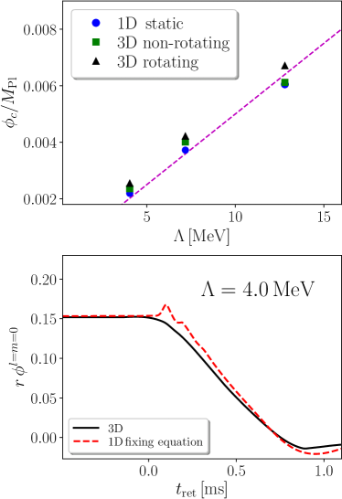
Fig. 1: Top: Central scalar field for rotating/non-rotating stars produced with our three-dimensional code and non-rotating ones produced with the static one-dimensional code of ter Haar et al. (2021). Stellar masses are $M\approx 1.74\,M_{\odot}$. Also shown is the expected linear scaling with $\Lambda$ Bezares et al. (2021b). Bottom: Scalar field at the extraction radius for gravitational collapse (with mass $M\approx 1.74\,M_{\odot}$), obtained with the one-dimensional code of Bezares et al. (2021b) (using an approximate fixing-equation approach) and our three-dimensional code.

Set-up: In order to perform fully relativistic numerical simulations of binary mergers in $k$-essence theory, we consider the Einstein frame and evolve the CCZ4 formulation Alic et al. (2012); Palenzuela et al. (2018); Bezares et al. (2017) of the Einstein equations (with the 1+log slicing Bona et al. (1995) and the Gamma-driver shift condition Alcubierre et al. (2003)) coupled to a perfect fluid (adopting an ideal-gas equation of state with $\Gamma=2$) Liebling et al. (2020) and a scalar field Bezares and Palenzuela (2018). Without loss of generality, we fix $\beta=0$ and $\gamma=1$, which ensure the well-posedness of the Cauchy problem Bezares et al. (2021a) and the existence of screening solutions ter Haar et al. (2021); Bezares et al. (2021b). Furthermore, we set the conformal coupling to $\alpha\approx 0.14$. As discussed in Bezares et al. (2021b), $\Lambda\sim\Lambda_{\mathrm{DE}}$ is intractable numerically due to the hierarchy between binary and cosmological scales (which leads to $\Lambda_{\mathrm{DE}}\sim 10^{-12}$ in units adapted to the binary system). Like in ter Haar et al. (2021); Bezares et al. (2021b), we study $\Lambda\gtrsim 1\,\mathrm{MeV}$ (for which screening is already present).

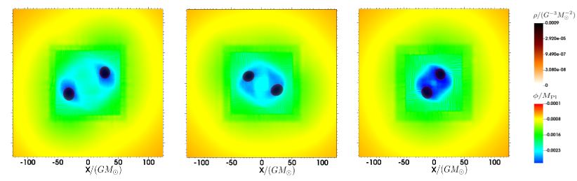
Fig. 2: Unequal-mass ($q=0.91$) NS binary with $\Lambda=4.0\,\rm{MeV}$, shown at successive times. The color code represents the scalar field, which is initially centered on each star and then develops into a common “envelope”, while the dark orange represents the fluid density.

The computational code, generated by using the platform Simflowny Arbona et al. (2013, 2018); sim (2021), runs under the SAMRAI infrastructure Hornung and Kohn (2002); Gunney and Anderson (2016); sam (2021), which provides parallelization and the adaptive mesh refinement (AMR) required to solve the different scales in the problem. We use fourth-order finite difference operators to discretize our equations Palenzuela et al. (2018). For the fluid and the scalar, we use High-Resolution Shock-Capturing (HRSC) methods to deal with shocks, as discussed in Bezares et al. (2021a); ter Haar et al. (2021); Bezares et al. (2021b). A similar GR code, using the same methods, has been recently used to simulate binary NSs Liebling et al. (2020, 2021). Our computational domain ranges from $[-1500,1500]^{3}\,\rm{km}$ and contains 6 refinement levels. Each level has twice the resolution of the previous one, achieving a resolution of $\Delta x_{6}=300\,\rm{m}$ on the finest grid. We use a Courant factor $\lambda_{c}\equiv\Delta t_{l}/\Delta x_{l}=0.4$ on each refinement level $l$ to ensure stability of the numerical scheme.

Isolated stars and gravitational collapse: We construct initial data for NS systems in $k$-essence theory by relaxation Barausse et al. (2013); Palenzuela et al. (2014), i.e. we generate GR solutions using LORENE lor (2010) and evolve them in $k$-essence until that they relax to stationary solutions. These solutions agree with the non-rotating solutions for $k$-mouflage stars found in ter Haar et al. (2021); Bezares et al. (2021b), thus validating our relaxation technique (Fig. 1, top panel). Similarly, we have also considered rotating solutions in $k$-essence, finding for the first time that (i) they behave qualitatively like the non-spinning ones, and (ii) the screening mechanism also survives in axisymmetry (Fig. 1, top panel). We also reproduced the dynamics of stellar oscillations in $k$-essence found in ter Haar et al. (2021); Bezares et al. (2021b), and managed to follow the (spherical) black-hole collapse of a NS (Fig. 1, bottom panel). These simulations were inaccessible, due to the diverging characteristic speeds, within the framework of ter Haar et al. (2021), without the addition of an extra driver field and a “fixing equation” Cayuso et al. (2017); Allwright and Lehner (2019) for it Bezares et al. (2021b). Here, using the gauge conditions mentioned above (and typically employed in numerical-relativity simulations of compact objects in 3+1 dimensions), we found no divergence of the characteristic speeds in our class of $k$-essence theories. The collapse obtained with this gauge matches exactly the results obtained in Bezares et al. (2021b), as shown in the bottom panel of Fig. 1, corroborating the (approximate) “fixing equation” technique employed there. We will therefore use the aforementioned gauge conditions throughout this paper.

Binary evolutions: Like in the isolated case, initial data for binary systems are constructed by relaxation. The relaxation process occurs approximately in the initial $4\,\rm{ms}$ of our simulations, and does not impact significantly the subsequent binary evolution. We consider binary NSs in quasi-circular orbits with a total gravitational mass $2.8-2.9\,M_{\odot}$ and mass ratio $q=M_{2}/M_{1}=[0.72,1]$. Time snapshots of a binary with mass ratio $q=0.9$ in a theory with $\Lambda\approx 4$ MeV are shown in Fig 2, displaying both the star’s density and the scalar field. The screening radii of the stars in isolation are $\sim 120$ km and thus larger than the initial system separation. This is the physically relevant situation, as for $\Lambda\sim\Lambda_{\rm DE}$ the screening radii are $\sim 10^{11}$ km. Also observe the formation of a scalar wake trailing each star (for the most part), with the two wakes merging in the last stages of the inspiral.

The response of a detector to the GW signal from NS binaries is encoded in the Newman-Penrose invariants in the Jordan frame Eardley et al. (1973), i.e. projections of the Riemann tensor on a null tetrad $l,n,m,\bar{m}$ adapted to outgoing waves. Tensor and scalar GWs are encoded respectively in $\psi_{4}=-R_{\ell\bar{m}\ell\bar{m}}=\Phi\,\tilde{\psi}_{4}$ and in $\phi_{22}=-R_{l{m}l\bar{m}}=\phi\,\left(\tilde{\phi}_{22}-l^{\nu}l^{\mu}\nabla_{\nu}\nabla_{\mu}\log\Phi/2+...\right)$, with a tilde denoting quantities in the Einstein frame (where we perform our simulation) and the dots denoting terms subleading in the distance $r$. We place our extraction radius outside the screening radius of the individual NSs, at distances of 300 km from the center of mass. This is justified because the distance to the detector is typically $\gg 10^{11}$ km, which is the screening radius for $\Lambda\sim\Lambda_{\rm DE}$, even for Galactic sources. In this regime, the amplitude of scalar perturbations decays as $1/r$, and therefore $\phi_{22}\approx-\alpha\sqrt{16\pi\,G}\partial_{t}^{2}\phi+O({1}/{r^{2}})$ Barausse et al. (2013); Bezares et al. (2021b).

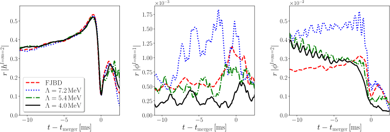
Fig. 3: Tensor ($l=m=2$) and scalar ($l=m=1$ and $l=m=2$) strain for a NS merger with $q=0.91$, in $k$-essence and FJBD.

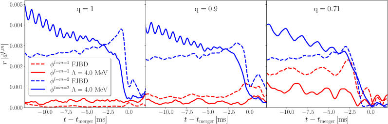
Fig. 4: Dipole ($l=m=1$) and quadrupole ($l=m=2$) scalar strain for merging NS binaries of varying mass ratio, in $k$-essence and FJBD.

The tensor and scalar “strains”, $h$ and $h_{s}$, are defined by integrating $\psi_{4}$ and $\phi_{22}$ twice in time, i.e. $\psi_{4}=\partial_{t}^{2}h/2$ and $\phi_{22}=\partial_{t}^{2}h_{s}$. The latter definition yields simply $h_{s}\propto\phi$ Gerosa et al. (2016). We then decompose $h$ and $h_{s}$ (or $\phi$) into spin-weighted spherical harmonics. As expected, the dominant contribution comes from the $\ell=m=2$ mode for the tensor strain. For the scalar emission the monopole $\ell=m=0$ is suppressed, and the main contribution comes from the dipole ($\ell=m=1$) mode and (mostly) the quadrupole ($\ell=m=2$) mode. The results for four simulations – for $\Lambda\approx 4$, 5 and 7 MeV and for FJBD (corresponding to $\Lambda\to\infty$), with $\alpha\approx 0.14$ – are shown in Fig. 3. Notice that we do not show the GR tensor strain as it is practically indistinguishable from the FJBD one on this timescale Barausse et al. (2013). The three values of $\Lambda$ predict screening radii larger than the initial separation between the stars.

As can be seen, the tensor strains are very similar, even after the merger (corresponding to the peak amplitude). As for the scalar, the suppression of the $\ell=m=0$ mode is expected, since monopole emission vanishes in FJBD theory for quasi-circular binaries Damour and Esposito-Farese (1992); Will and Zaglauer (1989). The $\ell=m=1$ dipole mode is instead small but non-vanishing, as expected for unequal-mass binaries in FJBD, with signs of screening suppression as $\Lambda$ decreases. However, the (dominant) $\ell=m=2$ scalar quadrupole mode is always larger than in FJBD theory, suggesting that the screening is not effective at suppressing the quadrupole scalar emission in the late inspiral/merger. The amplitude also seems to increase when going to low frequencies/early times, in the simulations with $\Lambda\approx 4$ and 5 MeV. Note that one does not expect a continuous limit to FJBD ($\Lambda\to\infty$) when $\Lambda$ increases. In FJBD there is no screening and the binary is always in the perturbative regime, while in $k$-essence the separation is always smaller than the screening radii. This is true even for observed binary pulsars, which have separations $\lesssim 10^{5}$ km vs screening radii of $\sim 10^{11}$ km for $\Lambda\sim\Lambda_{\rm DE}$.

The dependence on the mass ratio of the binary (which we set to $q=1$, 0.9 and 0.71) is shown in Fig. 4, for the FJBD and $\Lambda\approx 4$ MeV cases. As can be observed, quadrupole fluxes are largely unaffected by $q$ in both theories, with the $k$-essence ones consistently larger, especially at early times. The dipole fluxes in $k$-essence show again signs of suppression relative to FJBD, at least for $q\neq 1$, but in both theories they grow as $q$ decreases. This is expected, since PN calculations in FJBD Damour and Esposito-Farese (1992); Will and Zaglauer (1989) predict that the dipole amplitude should scale as the difference of the stellar scalar charges, which grows as $q$ decreases. For $q=1$, instead, the dipole flux in FJBD is compatible with zero (as predicted by PN theory Damour and Esposito-Farese (1992); Will and Zaglauer (1989)), while it does not vanish in $k$-essence.

Conclusions: We have performed for the first time fully relativistic simulations of binary NSs in theories of gravity with kinetic screening of local scales. We dealt with shocks in the scalar field by a HRSC method and by adopting a gauge with non-zero shift that prevents divergences of the characteristic speeds, which plagued previous attempts Bernard et al. (2019); Bezares et al. (2021a); ter Haar et al. (2021). With this setup, we have confirmed previous preliminary results by ourselves Bezares et al. (2021b), which were obtained with an approximate fixing-equation approach Cayuso et al. (2017); Allwright and Lehner (2019) and which hinted at a possible breakdown of the screening in black-hole collapse. In the late inspiral and merger of binary NSs, the (subdominant) dipole scalar emission is screened (at least for unequal masses), but the (dominant) quadrupole scalar flux is not. In fact, our results seem to hint at quadrupole scalar emission being as important (or even larger, especially at low frequencies) in $k$-essence than in FJBD theories with the same conformal coupling $\alpha$, as long as the strong-coupling scale is in the MeV range that we can simulate. If this feature survives for $\Lambda\sim\Lambda_{\rm DE}$, $k$-essence theories may become as fine-tuned as FJBD theory (which will wash out any effect on large-scale structure observations). Considering for instance the relativistic double-pulsar system $J0737-3039$ Kramer et al. (2006); Noutsos et al. (2020); Kramer et al. (2021), in FJBD the absence of scalar quadrupole radiation constrains $|\alpha|\lesssim 4.4\times 10^{-2}$.

Appendix A Appendix A: Covariant evolution equations

All the equations presented in this section are in the Einstein frame and therefore, to avoid the clutter of notation, we remove the tilde and leave it understood that all quantities are always in the Einstein frame. Notice, however, that the results of the convergence tests in the next section are converted back to the physical Jordan frame.

The equations of motion for the metric and scalar field can be obtained by varying the action (1) leading to

$$G_{\mu\nu}=8\pi G\big{(}T^{\phi}_{\mu\nu}+T_{\mu\nu}\big{)}\;,$$ (3)

$$\nabla_{\mu}\left[K^{\prime}(X)\nabla^{\mu}\phi\right]=\frac{1}{2}\mathcal{A}T\;,$$ (4)

where $G_{\mu\nu}$ is the Einstein tensor, $\mathcal{A}\equiv-\Phi^{\prime}(\phi)/[2\Phi(\phi)]$ and ‘prime’ denotes a derivative with respect to the argument in parenthesis. The scalar field and matter energy-momentum tensors are defined as

$$T^{\phi}_{\mu\nu} = K(X)g_{\mu\nu}-2K^{\prime}(X)\partial_{\mu}\phi\partial_{\nu}\phi\;,$$ (5)

$$T_{\mu\nu} = \frac{2}{\sqrt{-g}}\frac{\delta S_{m}}{\delta g_{\mu\nu}}\;,$$ (6)

with $T=T_{\mu\nu}g^{\mu\nu}$.

For our purposes, the matter is described by using the stress-energy tensor for a perfect fluid, namely

$$T_{\mu\nu}=[\rho_{0}(1+\epsilon)+P]u_{\mu}u_{\nu}+P\,g_{\mu\nu}\,,$$ (7)

where $\rho_{0}$ is the rest-mass density, $\epsilon$ its specific internal energy, $P$ is the pressure and $u_{\mu}$ its four-velocity.

Finally, the general relativistic hydrodynamics equations are given by

$$\nabla_{\mu}T^{\mu\nu} = \mathcal{A}\,T\,\nabla^{\nu}\phi\,,$$ (8)

$$\nabla_{\mu}(\rho_{0}u^{\mu}) = \rho_{0}\mathcal{A}\,u^{\mu}\nabla_{\mu}\phi\,.$$ (9)

Note that these are not conservation equations due to the coupling between the scalar field and matter.

We can now proceed to review the evolution equations for the metric, the scalar field and the matter, obtained by performing a 3+1 decomposition of the covariant equations.

A.1 Metric

The Einstein equations (3) are written as an evolution system by using the covariant conformal Z4 (CCZ4) formulation, which extends the Einstein equations by introducing a four-vector $Z_{\mu}$ as follows

$$R_{\mu\nu}+\nabla_{\mu}Z_{\nu}+\nabla_{\nu}Z_{\mu}=8\pi\,\Big{[}\left(T^{\phi}_{\mu\nu}+T_{\mu\nu}\right)$$ (10)

$$-\frac{1}{2}g_{\mu\nu}\,\left(T^{\phi}+T\right)\Big{]}+\kappa_{z}\,\left(n_{\mu}Z_{\nu}+n_{\nu}Z_{\mu}-g_{\mu\nu}n^{\sigma}Z_{\sigma}\right)\,,$$

where $\kappa_{z}>0$ is a damping term enforcing the dynamical decay of the constraint violations associated with $Z_{\mu}$ Gundlach et al. (2005).

As customary, we split the spacetime tensors and equations into their space and time components by using a $3+1$ decomposition. The line element is then given by

$$ds^{2}=-N^{2}\,dt^{2}+\gamma_{ij}\bigl{(}dx^{i}+\beta^{i}dt\bigr{)}\bigl{(}dx^{j}+\beta^{j}dt\bigr{)},$$ (11)

where $N$ is the lapse function, $\beta^{i}$ is the shift vector, and $\gamma_{ij}$ is the induced metric on each spatial foliation, denoted by $\Sigma_{t}$. In this foliation, we can define the normal to the hypersurfaces $\Sigma_{t}$ as $n_{\mu}=(-N,0)$ and the extrinsic curvature $K_{ij}\equiv-\frac{1}{2}\mathcal{L}_{n}\gamma_{ij}$, where $\mathcal{L}_{n}$ is the Lie derivative along $n^{\mu}$. By introducing a (spatial) conformal decomposition and some definitions, namely

$$\bar{\gamma}_{ij} = \chi\,\gamma_{ij}~{}~{},~{}~{}\bar{A}_{ij}=\chi\left(K_{ij}-\frac{1}{3}\gamma_{ij}\mathrm{tr}K\right),$$ (12)

$$\mathrm{tr}{\hat{K}} = \mathrm{tr}K-2\,\Theta~{}~{},~{}~{}{\hat{\Gamma}}^{i}={\bar{\Gamma}}^{i}+2Z^{i}/\chi,$$ (13)

where $\bar{\Gamma}^{i}=-\partial_{j}\bar{\gamma}^{ji}$, $\mathrm{tr}K=\gamma^{ij}K_{ij}$ and $\Theta\equiv-n_{\mu}Z^{\mu}$, one can obtain the final equations for the evolution fields $\{\chi,\bar{\gamma}_{ij},\mathrm{tr}{\hat{K}},\bar{A}_{ij},{\hat{\Gamma}}^{i},\Theta\}$. The explicit form of these equations is lengthy and can be found in Bezares et al. (2017). Note that the definitions above lead to new conformal constraints,

$$\bar{\gamma}=\det(\bar{\gamma}_{ij})=1\,,\qquad\mathrm{tr}{\bar{A}}=\bar{\gamma}^{ij}\bar{A}_{ij}=0,$$ (14)

which can also be enforced dynamically by including additional damping terms proportional to $\kappa_{c}>0$ in the evolution equations. Finally, we supplement these equations with gauge conditions for the lapse and shift. We use the 1+log slicing condition Bona et al. (1995) and the Gamma-driver shift condition Alcubierre et al. (2003), namely

$$\partial_{t}N = \beta^{k}\partial_{k}N-N^{2}f(N)\mathrm{tr}{\hat{K}}\,,$$ (15)

$$\partial_{t}\beta^{i} = \beta^{k}\partial_{k}\beta^{i}+\eta\beta^{i}-N^{2}g(N){\hat{\Gamma}}^{i}\,,$$ (16)

being $f(N)$ and $g(N)$ arbitrary functions depending on the lapse, and $\eta$ a constant parameter. In our case, a successful choice is $f(N)=2/N$, $g(N)=3/(4N^{2})$ and $\eta=2$.

A.2 Scalar field

The time evolution equation for the scalar field can also be obtained by performing a 3+1 decomposition on Eq. (4). Due to the genuinely non-linear character of this equation, shocks might appear during the evolution, even if the initial data is smooth. This problem is also present in fluid dynamics, where it is solved by considering the weak (or integral) balance law form of the equations and then by using suitable High-Resolution-Shock-Capturing (HRSC) numerical methods to solve them. We follow here the same procedure, writing Eq. (4) in balance law form

$$\partial_{t}\vec{\mathcal{U}}+\partial_{i}F^{i}(\vec{\mathcal{U}})=S(\vec{\mathcal{U}})\;,$$ (17)

where $\vec{\mathcal{U}}$ is a vector containing all the conserved or evolved fields, $F^{i}(\vec{\mathcal{U}})$ are the fluxes and $S(\vec{\mathcal{U}})$ the sources. Notice that neither the fluxes nor the sources contain derivatives of the evolved fields.

By defining the following new evolved fields

$$\phi_{i} \equiv \partial_{i}\phi~{},$$ (18)

$$\Pi \equiv -n_{\mu}\partial^{\mu}\phi=-\frac{1}{N}(\partial_{t}\phi-\beta^{i}\phi_{i})~{},$$ (19)

the evolution equations for the scalar field in terms of the 3+1 quantities can be written as

$$\partial_{t}\phi = \beta^{k}\phi_{k}-N\Pi~{},$$ (20)

$$\partial_{t}\phi_{i} = -\partial_{i}(-\beta^{k}\phi_{k}+N\Pi)~{},$$ (21)

$$\partial_{t}(\sqrt{\gamma}\Psi) = -\partial_{k}[\sqrt{\gamma}(-\beta^{k}\Psi+NK^{\prime}(X)\gamma^{kj}\phi_{j})]$$ (22)

$$+\frac{1}{2}N\sqrt{\gamma}\mathcal{A}T~{},$$

where $\gamma=\det(\gamma_{ij})$ and $\Psi=K^{\prime}(X)\Pi.$

Therefore, our conservative evolved fields are $\{\phi,\phi_{i},\Psi\}$, while the primitive physical variables required to compute the fluxes and sources are given by $\{\phi,\phi_{i},\Pi\}$. In order to calculate $\Pi$ from $\Psi$, the following non-linear equation

$$K^{\prime}(X)\Pi-\Psi=0$$ (23)

must be resolved numerically (for instance with a Newton-Raphson method) at each time-step.

A.3 Matter

The general relativistic hydrodynamics equations are written in flux-conservative form as well, i.e.

$$\partial_{t}(\sqrt{\gamma}D)+\partial_{k}[\sqrt{\gamma}D(Nv^{k}-\beta^{k})] = N\mathcal{A}\sqrt{\gamma}D(-\Pi+v^{k}\phi_{k})\,,$$ (24)

$$\partial_{t}(\sqrt{\gamma}\tau)+\partial_{k}[\sqrt{\gamma}(-\beta^{k}\tau+N[S^{k}-Dv^{k}])] = N\sqrt{\gamma}\mathcal{A}\left[\Pi T+\Pi D-v^{k}\phi_{k}D\right]+\sqrt{\gamma}\left[NS^{ij}K_{ij}-S^{i}\partial_{i}N\right]\,,$$ (25)

$$\partial_{t}(\sqrt{\gamma}S_{i})+\partial_{k}[\sqrt{\gamma}(-\beta^{k}S_{i}+NS^{k}_{i})] = N\sqrt{\gamma}\mathcal{A}\left[\phi_{i}T\right]+\sqrt{\gamma}\left[N\Gamma^{j}_{ik}S^{k}_{j}+S_{j}\partial_{i}\beta^{j}-(\tau+D)\partial_{i}N\right]\,,$$ (26)

where $v^{i}$ is the fluid velocity measured by an Eulerian observer

$$v^{i} = \frac{u^{i}}{W}+\frac{\beta^{i}}{N},$$ (27)

with $W\equiv 1/\sqrt{1-\gamma^{ij}v_{i}v_{j}}$ the Lorentz factor. The evolved conserved variables in this case are the rest-mass density measured by an Eulerian observer ($D$), the energy density (with the exclusion of the mass density) ($\tau$) and the momentum density ($S_{i}$), which are defined in terms of the primitive field as follows:

$$D = \rho W~{},$$ (28)

$$\tau = hW^{2}-p-D~{},$$ (29)

$$S_{i} = hW^{2}v_{i}~{},$$ (30)

$$S_{ij} = \frac{1}{2}\left(v_{i}S_{j}+v_{j}S_{i}\right)+\gamma_{ij}P~{},$$ (31)

being $h=\rho_{0}(1+\epsilon)+P$ the enthalpy. Again, the relation between the evolved and the primitive fields is nonlinear and it needs to be solved numerically by using a Newton-Raphson method in order to calculate the fluxes and sources.

Appendix B Appendix B: Code validation

The validity of our 3+1 evolution code evolving NSs in $k$-essence theory has been checked with two types of tests. First, we compared our simulations with solutions obtained by solving for static NSs in spherical symmetry. We also compared with simulations of perturbed stars, which were performed with an independent 1+1 code in spherical symmetry ter Haar et al. (2021); Bezares et al. (2021b). Here, we considered not only small oscillations, but also cases where stellar perturbations are large enough to induce the gravitational collapse of the star to a black hole. All these results are summarized briefly in the main text, and will not be repeated here. Second, we have performed standard convergence tests both for these isolated NS solutions, as well as for the binary NS coalescence simulations.

The first convergence test was performed for an isolated non-rotating NS with $\Lambda=4.0~{}\rm{MeV}$. We consider three different resolutions (i.e. low, medium and high) such that the star is covered roughly with $N=(66,82,103)$ points respectively. As described in the main text, our simulations begin from a NS solution in GR, which relaxes dynamically to a $k$-essence solution. We display the value of the scalar field at the center of the star in the top panel of Fig. 5 for our three resolutions, showing that they all tend to the same value, which is very close to the one obtained with the 1+1 spherically symmetric code. Furthermore, the L2-norm of the Hamiltonian constraint for the three previous resolutions is displayed in the bottom panel of Fig. 5, showing a convergence between third and fourth order.

The second convergence test was performed for one of our unequal binary NS simulations with mass ratio $q=0.9$, using again $\Lambda=4.0~{}\rm{MeV}$. We consider three resolutions $\Delta x=(366,292,232)~{}\rm{m}$, such that each star is covered roughly by $N=(80,100,126)$ points. In the top panel of Fig. 6 the L2-norm of the Hamiltonian constraint is displayed for these resolutions. The middle panel displays the main quadrupolar mode $l=m=2$ of the GW signal. The differences between simulations decrease as the resolution increases. This is more evident from the bottom panel, where phase differences are displayed. Both the waveforms and the constraint converge, after the initial relaxation time and until almost the merger time, at least to second order.

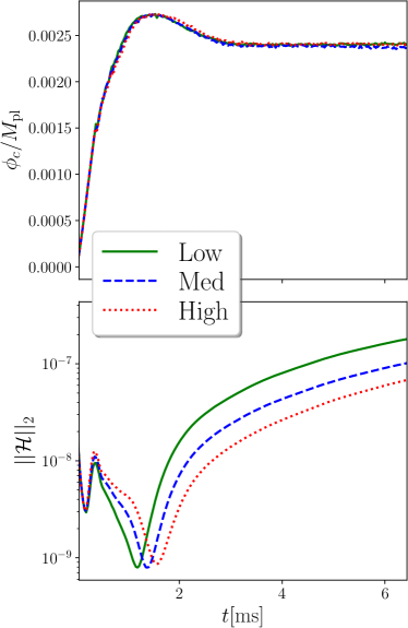
Fig. 5: Isolated non-rotating NSs. Top: Central value of the scalar field. The NS is initially a solution of Einstein equations, but it relaxes to the k-essence solution dynamically. We considered three different resolutions covering the star with $N=(80,100,126)$ points. Bottom: L₂-norm of the Hamiltonian constraint for the three different resolutions above. After the transient initial relaxation, these solutions show between third and fourth order convergence.

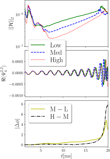
Fig. 6: Binary NS simulations. Top: The L2-norm of the Hamiltonian constraint for three resolutions $\Delta x=(366,292,232)~{}\rm{m}$. Middle: Main quadrupolar mode of the $\Psi_{4}$ for the three resolutions. Bottom: Difference between the phase of the different resolutions. The solutions converge at least at second order after the transient relaxation (from the GR solution to the $k$-essence one) and until the merger.

References

- Abbott et al. (2016) B. P. Abbott et al. (LIGO Scientific, Virgo), Phys. Rev. Lett. 116, 221101 (2016), [Erratum: Phys.Rev.Lett. 121, 129902 (2018)], arXiv:1602.03841 [gr-qc] .
- Abbott et al. (2019a) B. P. Abbott et al. (LIGO Scientific, Virgo), Phys. Rev. Lett. 123, 011102 (2019a), arXiv:1811.00364 [gr-qc] .
- Abbott et al. (2019b) B. Abbott et al. (LIGO Scientific, Virgo), Phys. Rev. D 100, 104036 (2019b), arXiv:1903.04467 [gr-qc] .
- Abbott et al. (2020) R. Abbott et al. (LIGO Scientific, Virgo), (2020), arXiv:2010.14529 [gr-qc] .
- Will (2014) C. M. Will, Living Rev. Rel. 17, 4 (2014), arXiv:1403.7377 [gr-qc] .
- Damour and Taylor (1992) T. Damour and J. H. Taylor, Phys. Rev. D45, 1840 (1992).
- Kramer et al. (2006) M. Kramer et al., Science 314, 97 (2006), arXiv:astro-ph/0609417 [astro-ph] .
- Freire et al. (2012) P. C. C. Freire, N. Wex, G. Esposito-Farese, J. P. W. Verbiest, M. Bailes, B. A. Jacoby, M. Kramer, I. H. Stairs, J. Antoniadis, and G. H. Janssen, Mon. Not. Roy. Astron. Soc. 423, 3328 (2012), arXiv:1205.1450 [astro-ph.GA] .
- Fierz (1956) M. Fierz, Helv. Phys. Acta 29, 128 (1956).
- Jordan (1959) P. Jordan, Z. Phys. 157, 112 (1959).
- Brans and Dicke (1961) C. Brans and R. H. Dicke, Phys. Rev. 124, 925 (1961).
- Babichev et al. (2009) E. Babichev, C. Deffayet, and R. Ziour, Int. J. Mod. Phys. D 18, 2147 (2009), arXiv:0905.2943 [hep-th] .
- Vainshtein (1972) A. Vainshtein, Phys. Lett. B 39, 393 (1972).
- Clifton et al. (2012) T. Clifton, P. G. Ferreira, A. Padilla, and C. Skordis, Phys. Rept. 513, 1 (2012), arXiv:1106.2476 [astro-ph.CO] .
- Koyama (2016) K. Koyama, Rept. Prog. Phys. 79, 046902 (2016), arXiv:1504.04623 [astro-ph.CO] .
- Babichev et al. (2010) E. Babichev, C. Deffayet, and R. Ziour, Phys. Rev. D82, 104008 (2010), arXiv:1007.4506 [gr-qc] .
- Babichev and Crisostomi (2013) E. Babichev and M. Crisostomi, Phys. Rev. D88, 084002 (2013), arXiv:1307.3640 [gr-qc] .
- de Rham et al. (2013a) C. de Rham, A. Matas, and A. J. Tolley, Phys. Rev. D 87, 064024 (2013a), arXiv:1212.5212 [hep-th] .
- de Rham et al. (2013b) C. de Rham, A. J. Tolley, and D. H. Wesley, Phys. Rev. D 87, 044025 (2013b), arXiv:1208.0580 [gr-qc] .
- Dar et al. (2019) F. Dar, C. D. Rham, J. T. Deskins, J. T. Giblin, and A. J. Tolley, Class. Quant. Grav. 36, 025008 (2019), arXiv:1808.02165 [hep-th] .
- Crisostomi and Koyama (2018) M. Crisostomi and K. Koyama, Phys. Rev. D 97, 021301 (2018), arXiv:1711.06661 [astro-ph.CO] .
- Abbott et al. (2017a) B. Abbott et al. (LIGO Scientific, Virgo, Fermi-GBM, INTEGRAL), Astrophys. J. Lett. 848, L13 (2017a), arXiv:1710.05834 [astro-ph.HE] .
- Abbott et al. (2017b) B. Abbott et al. (LIGO Scientific, Virgo), Phys. Rev. Lett. 119, 161101 (2017b), arXiv:1710.05832 [gr-qc] .
- Creminelli et al. (2018) P. Creminelli, M. Lewandowski, G. Tambalo, and F. Vernizzi, JCAP 1812, 025 (2018), arXiv:1809.03484 [astro-ph.CO] .
- Creminelli et al. (2020) P. Creminelli, G. Tambalo, F. Vernizzi, and V. Yingcharoenrat, JCAP 2005, 002 (2020), arXiv:1910.14035 [gr-qc] .
- Babichev (2020) E. Babichev, JHEP 07, 038 (2020), arXiv:2001.11784 [hep-th] .
- Wagoner (1970) R. V. Wagoner, Phys. Rev. D 1, 3209 (1970).
- Chiba et al. (2000) T. Chiba, T. Okabe, and M. Yamaguchi, Phys. Rev. D62, 023511 (2000), arXiv:astro-ph/9912463 [astro-ph] .
- Armendariz-Picon et al. (2000) C. Armendariz-Picon, V. F. Mukhanov, and P. J. Steinhardt, Phys. Rev. Lett. 85, 4438 (2000), arXiv:astro-ph/0004134 [astro-ph] .
- Hui and Nicolis (2013) L. Hui and A. Nicolis, Phys. Rev. Lett. 110, 241104 (2013), arXiv:1202.1296 [hep-th] .
- Detweiler (1980) S. L. Detweiler, Phys. Rev. D 22, 2323 (1980).
- Healy et al. (2012) J. Healy, T. Bode, R. Haas, E. Pazos, P. Laguna, D. Shoemaker, and N. Yunes, Class. Quant. Grav. 29, 232002 (2012), arXiv:1112.3928 [gr-qc] .
- Jacobson (1999) T. Jacobson, Phys. Rev. Lett. 83, 2699 (1999), arXiv:astro-ph/9905303 .
- Bernard et al. (2019) L. Bernard, L. Lehner, and R. Luna, Phys. Rev. D 100, 024011 (2019), arXiv:1904.12866 [gr-qc] .
- Bezares et al. (2021a) M. Bezares, M. Crisostomi, C. Palenzuela, and E. Barausse, JCAP 2103, 072 (2021a), arXiv:2008.07546 [gr-qc] .
- de Rham and Ribeiro (2014) C. de Rham and R. H. Ribeiro, JCAP 1411, 016 (2014), arXiv:1405.5213 [hep-th] .
- Brax and Valageas (2016) P. Brax and P. Valageas, Phys. Rev. D94, 043529 (2016), arXiv:1607.01129 [astro-ph.CO] .
- Figueras and França (2020) P. Figueras and T. França, Class. Quant. Grav. 37, 225009 (2020), arXiv:2006.09414 [gr-qc] .
- ter Haar et al. (2021) L. ter Haar, M. Bezares, M. Crisostomi, E. Barausse, and C. Palenzuela, Phys. Rev. Lett. 126, 091102 (2021), arXiv:2009.03354 [gr-qc] .
- Bezares et al. (2021b) M. Bezares, L. ter Haar, M. Crisostomi, E. Barausse, and C. Palenzuela, (2021b), arXiv:2105.13992 [gr-qc] .
- Courant et al. (1928) R. Courant, K. Friedrichs, and H. Lewy, Mathematische Annalen 100, 32 (1928).
- Cayuso et al. (2017) J. Cayuso, N. Ortiz, and L. Lehner, Phys. Rev. D 96, 084043 (2017), arXiv:1706.07421 [gr-qc] .
- Allwright and Lehner (2019) G. Allwright and L. Lehner, Class. Quant. Grav. 36, 084001 (2019), arXiv:1808.07897 [gr-qc] .
- Cayuso and Lehner (2020) R. Cayuso and L. Lehner, Phys. Rev. D 102, 084008 (2020), arXiv:2005.13720 [gr-qc] .
- Alic et al. (2012) D. Alic, C. Bona-Casas, C. Bona, L. Rezzolla, and C. Palenzuela, Phys. Rev. D 85, 064040 (2012), arXiv:1106.2254 [gr-qc] .
- Palenzuela et al. (2018) C. Palenzuela, B. Miñano, D. Viganò, A. Arbona, C. Bona-Casas, A. Rigo, M. Bezares, C. Bona, and J. Massó, Class. Quant. Grav. 35, 185007 (2018), arXiv:1806.04182 [physics.comp-ph] .
- Bezares et al. (2017) M. Bezares, C. Palenzuela, and C. Bona, Phys. Rev. D 95, 124005 (2017), arXiv:1705.01071 [gr-qc] .
- Bona et al. (1995) C. Bona, J. Masso, E. Seidel, and J. Stela, Phys. Rev. Lett. 75, 600 (1995), arXiv:gr-qc/9412071 .
- Alcubierre et al. (2003) M. Alcubierre, B. Bruegmann, P. Diener, M. Koppitz, D. Pollney, E. Seidel, and R. Takahashi, Phys. Rev. D 67, 084023 (2003), arXiv:gr-qc/0206072 .
- Liebling et al. (2020) S. L. Liebling, C. Palenzuela, and L. Lehner, Class. Quant. Grav. 37, 135006 (2020), arXiv:2002.07554 [gr-qc] .
- Bezares and Palenzuela (2018) M. Bezares and C. Palenzuela, Class. Quant. Grav. 35, 234002 (2018), arXiv:1808.10732 [gr-qc] .
- Davis and Melville (2021) A.-C. Davis and S. Melville, (2021), arXiv:2107.00010 [gr-qc] .
- Aoki et al. (2021) K. Aoki, S. Mukohyama, and R. Namba, (2021), arXiv:2107.01755 [hep-th] .
- Arbona et al. (2013) A. Arbona, A. Artigues, C. Bona-Casas, J. Massó, B. Miñano, A. Rigo, M. Trias, and C. Bona, Computer Physics Communications 184, 2321 (2013).
- Arbona et al. (2018) A. Arbona, B. Miñano, A. Rigo, C. Bona, C. Palenzuela, A. Artigues, C. Bona-Casas, and J. Massó, Computer Physics Communications 229, 170 (2018).
- sim (2021) “Simflowny project website.” (2021).
- Hornung and Kohn (2002) R. D. Hornung and S. R. Kohn, Concurrency and Computation: Practice and Experience 14, 347 (2002).
- Gunney and Anderson (2016) B. T. Gunney and R. W. Anderson, Journal of Parallel and Distributed Computing 89, 65 (2016).
- sam (2021) “Samrai project website.” (2021).
- Liebling et al. (2021) S. L. Liebling, C. Palenzuela, and L. Lehner, Classical and Quantum Gravity 38, 115007 (2021).
- Barausse et al. (2013) E. Barausse, C. Palenzuela, M. Ponce, and L. Lehner, Phys. Rev. D 87, 081506 (2013), arXiv:1212.5053 [gr-qc] .
- Palenzuela et al. (2014) C. Palenzuela, E. Barausse, M. Ponce, and L. Lehner, Phys. Rev. D 89, 044024 (2014), arXiv:1310.4481 [gr-qc] .
- lor (2010) “Lorene home page,” (2010), http://www.lorene.obspm.fr/.
- Eardley et al. (1973) D. M. Eardley, D. L. Lee, and A. P. Lightman, Phys. Rev. D 8, 3308 (1973).
- Gerosa et al. (2016) D. Gerosa, U. Sperhake, and C. D. Ott, Class. Quant. Grav. 33, 135002 (2016), arXiv:1602.06952 [gr-qc] .
- Damour and Esposito-Farese (1992) T. Damour and G. Esposito-Farese, Class. Quant. Grav. 9, 2093 (1992).
- Will and Zaglauer (1989) C. M. Will and H. W. Zaglauer, Astrophys. J. 346, 366 (1989).
- Noutsos et al. (2020) A. Noutsos et al., Astron. Astrophys. 643, A143 (2020), arXiv:2011.02357 [astro-ph.HE] .
- Kramer et al. (2021) M. Kramer et al., Phys. Rev. X 11, 041050 (2021), arXiv:2112.06795 [astro-ph.HE] .
- Gundlach et al. (2005) C. Gundlach, J. M. Martin-Garcia, G. Calabrese, and I. Hinder, Class. Quant. Grav. 22, 3767 (2005), arXiv:gr-qc/0504114 .