The role of complex ionized absorber in the soft X-ray spectra of Intermediate Polars

Abstract

In magnetic Cataclysmic Variables (mCVs), X-ray radiation originates from the shock heated multi-temperature plasma in the post-shock region near the white dwarf surface. These X-rays are modified by a complex distribution of absorbers in the pre-shock region. The presence of photo-ionized lines and warm absorber features in the soft X-ray spectra of these mCVs suggests that these absorbers are ionized. We developed the ionized complex absorber model zxipab, which is represented by a power-law distribution of ionized absorbers in the pre-shock flow. Using the ionized absorber model zxipab along with a cooling flow model and a reflection component, we model the broadband Chandra/HETG and NuSTAR spectra of two IPs: NY Lup and V1223 Sgr. We find that this model describes well many of the H and He like emission lines from medium Z elements, which arises from the collisionally excited plasma. However the model fails to account for some of the He like triplets from medium Z elements, which points towards its photo-ionization origin. We do not find a compelling evidence for a blackbody component to model the soft excess seen in the residuals of the Chandra/HETG spectra, which could be due to the uncertainties in estimation of the interstellar absorption of these sources using Chandra/HETG data and/or excess fluxes seen in some photo-ionized emission lines which are not accounted by the cooling flow model. We describe the implications of this model with respect to the geometry of the pre-shock region in these two IPs.

1 Introduction

Cataclysmic Variables (CVs) are interacting binaries consisting of a white dwarf accreting matter from a low mass companion (usually a late type main sequence star; see review by Mukai 2017). The accretion flows around the white dwarfs are primarily governed by their magnetic fields. For non-magnetic CVs, the accretion disks extends upto the surface of the primary, whereas for polars the magnetic field is strong enough to prevent the formation of the accretion disk. Intermediate Polars (IPs) are a subclass of magnetic CVs, where a partial accretion disk exists and the accretion onto the white dwarf is magnetically funnelled onto their poles from the inner edge of the truncated accretion disks.

The X-ray emission from these IPs arises from the accreted matter shock heated up to high temperatures (kT $\sim$ 10–50 keV) and must cool before settling onto the surface of the white dwarf. The emergent X-ray spectrum is expected to be the resultant emission from plasmas over a continuous temperature distribution, from the shock temperature to the white dwarf photospheric temperature. High resolution X-ray spectra of CVs are found to be similar to the cooling flows spectra seen in clusters of galaxies (Fabian & Nulsen, 1977; Fabian, 1994). However, the low temperature emission predicted by the classical cooling flow models is absent in clusters of galaxies (see, e.g., Peterson et al. 2003) due to the presence of heating processes, presumably AGN feedback. On the other hand in CVs, cooling continues until the plasma reaches the white dwarf photospheric temperature (T $\sim$ 10⁴ K). The emergent X-rays from this shock heated multi-temperature plasma is modified by the presence of a complex distribution of absorbers in the pre-shock region. This complex absorber is expected to be ionized due to irradiation of the pre-shock flow around the white dwarf. For some IPs, a soft component is seen in the X-ray spectra which (in low to medium resolution data) is modelled by a blackbody with a temperature kT $\geq$ 60 eV (Evans & Hellier, 2007; Anzolin et al., 2008). This soft component is thought to arise from reprocessing of the hard X-rays, although there is a considerable uncertainty in the presence of this component.

The X-ray spectra of IPs are often strongly absorbed at a level significantly above the intervening interstellar column. Both the energy dependence of spin modulation amplitudes and the spectral shape of the spin phase-averaged spectra indicate that a simple absorber is not sufficient (Norton & Watson, 1989); these authors used the partial-covering absorber model pcfabs available in XSPEC. In pcfabs, some fraction of the emission is assumed to be observed directly, while the rest (“covering fraction”) is seen through a neutral absorber of column N_H. However, Done & Magdziarz (1998) pointed out that the partial covering absorber model is far too simplistic for the magnetic CVs. This is because the post-shock region, the source of the X-ray emision, is directly adjacent to the pre-shock flow, the site of the complex absorption. This results in an absorber having a continuous range of N_H, each value with its own differential covering fraction (see Figure 8 of Mukai 2017). Done & Magdziarz (1998) proposed to model this using a model in which the differential covering fraction is a power-law function of N_H, and encoded this in an XSPEC model pwab.

In this paper, we propose a further modification of the pwab model, because the accretion flow just above the shock is likely ionized. Photo-ionization model is usually calculated in terms of a cloud of density $n$ at a distance $r$ from the ionizing source with a luminosity of $L$ as $\xi=L/nr^{2}$. This can be generalized as the ratio of ionizing flux to density, modulo geometrical factor 4$\pi$, when considering an extended cloud neighboring an extended source of ionizing flux. For the pre-shock accretion flow in magnetic CVs, $\xi$ probably exceeds 10 just above the shock but rapidly decreases away from the shock front, due to the combination of geometrical dilution of the ionizing radiation (see Discussion). Observationally, the 0.73 keV edge due to O_VII has been detected in V1223 Sgr (Mukai, 2017) and in V2731 Oph (de Martino et al., 2008). It is likely that the pre-shock flow is the site for both the ionized absorbers and the photo-ionized emission features originally recognized by Mukai et al. (2003) and confirmed here in this work for NY Lup and V1223 Sgr.

The outline of the paper is as follows: in Section 2 we describe the Chandra/HETG and NuSTAR observations of NY Lup and V1223 Sgr. The broad-band X-ray Chandra/HETG and NuSTAR spectra is fitted by the complex absorption model zxipab which is described in detail in the Appendix. We discuss these results in Section 3.

2 Observations and Analysis

Table 1: Summary of X-ray observations

Source	Telescope	ObsID	Start Time	Exposure (kilosec)
NY Lup	Chandra/ACIS-S HETG	17874	2016-05-23 15:24:24	49.41
	Chandra/ACIS-S HETG	18857	2016-05-24 22:04:15	32.35
	Chandra/ACIS-S HETG	18858	2016-05-25 22:32:09	23.15
	Chandra/ACIS-S HETG	18859	2016-05-28 13:14:07	26.71
	NuSTAR	30001146002	2014-08-09 14:51:07	23.0
V 1223 Sgr	Chandra/ACIS-S HETG	649	2000-04-30 16:19:51	51.5
	NuSTAR	30001144002	2014-09-16 02:26:07	20.4

V1223 Sgr and NY Lup have been observed by Chandra ACIS-S camera and High Energy Transmission Grating (HETG; Canizares et al. 2005). HETG consists of two transmission gratings, Medium Energy Grating (MEG) and High Energy Grating (HEG), having absolute wavelength accuracy of 0.0006 Å and 0.011 Å respectively. To model the broadband X-ray spectra, we use the NuSTAR observations of V1223 Sgr and NY Lup, which have been previously analysed in Mukai et al. (2015) and Hayashi et al. (2021). The Nuclear Spectroscopic Telescope Array (NuSTAR; Harrison et al. 2013) carries two co-aligned Wolter I telescopes that focus X-rays between 3 and 79 keV onto two independent solid state Focal Plane Modules (FPMA and FPMB). Table 1 gives a summary of the X-ray observations of V1223 Sgr and NY Lup used in this paper.

The Chandra/HETG observations were downloaded from the Chandra archive and were processed by CIAO 4.12 and CALDB 4.9.4. The spectral products, response matrices and ancillary files for different grating orders were obtained by running the CIAO tool chandra$\_$repro script. The positive and negative diffraction first order spectra and their corresponding response files were co-added using the CIAO tool combine$\_$grating$\_$spectra. The first order spectra extracted from the multiple Chandra/HETG observations of NY Lup was also co-added using CIAO tool combine$\_$grating$\_$spectra. The NuSTAR data were processed by NuSTARDAS with the latest CALDB files. The source region was defined using a 100” circular region and the background region was also defined using a 100” circular region in a source-free region on the same detector. The spectral products, response matrices and ancillary files were obtained by nuproducts. The NuSTAR spectra were grouped with grppha to have atleast 30 counts per bin. Even though the NuSTAR and Chandra/HETG observations were carried out at different dates, we expect a similarity in the spectral shapes, which is determined by the gravitational potential just above the WD surface (Shaw et al., 2018). Therefore, small changes in overall accretion rate lead to small changes in overall normalization without spectral variations, as seen for V2731 Oph (Lopes de Oliveira & Mukai, 2019). The changes in the normalization is accounted by the cross-normalization constant of the spectral fits.

2.1 Simultaneous X-ray spectral fitting of Chandra/HETG and NuSTAR spectra

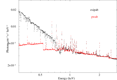
Figure 1: Model spectra using zxipab and pwab as the complex absorption model for V1223 Sgr with a log xi of 0.5.

The post-shock plasma in many mCVs can be well represented by the cooling flow model (Done et al., 1995; Mukai et al., 2003), which contains bremsstrahlung continuum and collisionally excited emission lines from a range of temperatures, with a distribution of emission measures appropriate for isobarically cooling plasma. Along with a multi-temperature plasma and photo-ionized emission lines, there are strong spectral signatures of reflection detected in NY Lup and V1223 Sgr (Mukai et al., 2015). Hayashi et al. (2021) also studied the reflection in V1223 Sgr using the Suzaku and NuSTAR data and their own model of multi-temperature emission and a reflection component.

The broadband Chandra/HETG and NuSTAR X-ray spectra of NY Lup and V1223 Sgr are fitted with a cooling flow model for the primary emission (mkcflow in XSPEC), a reflection model for the spectral signatures of a Compton hump (reflect in XSPEC) and a complex absorption model. The X-ray spectra, especially at lower energies, is modified by a complex distribution of absorbers in the pre-shock flow, which can be represented as a power-law distribution of neutral absorbers (pwab in XSPEC) (Done & Magdziarz, 1998). However, the X-ray emission is capable of ionizing the pre-shock flow, hence we expect these complex absorbers to be ionized. Therefore we developed a zxipab model as a local model in XSPEC, which is a power-law distribution of ionized absorbers. The complex ionized absorber model zxipab is similar to pwab except the ionization parameter log xi gives an indication of degree of ionization of the absorbers in the pre-shock region. The details of the zxipab model are given in the Appendix. We fit the Chandra/HETG spectra of NY Lup and V1223 Sgr with the ionized absorber zxipab model and compare it with the fits using a neutral absorber pwab model. A gaussian line was used to model the Fe K$\alpha$ line in the spectra, along with a gaussian smoothing model gsmooth to account for velocity broadening of emission lines. The power of energy for sigma variation ($\alpha$) of the gsmooth model is fixed to 1.0. In our spectral fits to the data, we do not detect significant interstellar absorption. This may be because the interstellar N_H for these objects are too low to be securely detected in the spectral fits, given the complexity of source spectrum and the calibration of the time-dependent low-energy effective area of Chandra/HETG/ACIS-S. The upper limits on interstellar absorption towards NY Lup is 1.4$\times 10^{21}$ cm^-2 (de Martino et al., 2008) and V1223 Sgr is 1$\times 10^{21}$ cm^-2 (Beuermann et al., 2004).

In XSPEC notation, the model is written as:
constant*complex*gsmooth(reflect*mkcflow+gaussian) where complex is pwab or zxipab. Figure 1 is the plot of the model spectra using zxipab and pwab as the complex absorption model for V1223 Sgr with a log xi of 0.5. We see a difference in the prediction between these two complex absorption models at energies below 0.8 keV, along with the presence of absorption lines in the model spectra using an ionized absorber zxipab model. Due to limited effective area and energy resolution of Chandra/HETG, we are unable to see these absorption lines in the spectra as well as the difference in the model prediction of fluxes by zxipab and pwab, especially below 0.5 keV. As shown later in Section 2.2, we see presence of various photo-ionized emission lines in the Chandra/HETG spectra of NY Lup and V1223 Sgr.

The Chandra/HETG spectra was fitted in energy range 0.5–7.5 keV and NuSTAR/FPMA + FPMB spectra in 3–40 keV. A constant was added for simultaneous Chandra/HETG, NuSTAR/FPMA + FPMB spectral fit to account for cross-normalization difference between the different instruments. We used chi-square statistics for fitting the Chandra/HETG and NuSTAR data in XSPEC v12.11.0. The abundance table was used from Asplund et al. (2009). The abundances of the cooling flow model was linked to the reflection model and was allowed to vary during the fit. The lowest temperature to which the plasma cools (kT_min of the mkcflow model) was fixed to its hard limit of 80.8 eV and the spectrum was calculated by using AtomDB data (switch=2 in mkcflow model). The inclination angle of the reflecting surface of the reflect model is fixed to cos $\mu$=0.45. The value of spectral parameters obtained by the spectral fits to only NuSTAR data of NY Lup and V1223 Sgr are similar to that reported in Mukai et al. (2015). Table 2 gives the spectral parameter of the best fit to the Chandra/HETG and NuSTAR spectral fits using the two complex absorption models: pwab and zxipab. The errors are calculated at 90% confidence limit.

Figure 2 compares the complex absorption models pwab and zxipab with that of the Chandra/HETG spectra of NY Lup and V1223 Sgr. We see a sharp discontinuity at the OVII edge around $\sim$ 0.9 keV in the Chandra/HETG spectra, which indicates the presence of warm absorber features (Mukai, 2017). Although the ionization parameter for NY Lup and V1223 Sgr is not very large, we still expect the pre-shock flow to be ionized due to high X-ray fluxes from these systems. The ionized absorber model zxipab is shown to fit the Chandra/HETG data better than the neutral absorber pwab model, especially at lower energies. However due to limited sensitivity of Chandra/HETG below 0.5 keV, we do not see a significant change in the fitting statistics between the two complex absorber models as expected from Figure 1.

We see residuals to the fit at lower energies in the lower panel of Figure 2. This soft excess is less for the ionized absorber model compared to the neutral absorber model. Some of these residuals are from the photo-ionized emission lines whose fluxes do not match the model predictions of the cooling flow model, described in detail in Section 2.2. We fit this soft excess with a black-body component and find that the estimated temperature is higher than the previously estimated temperature of 60 eV (Evans & Hellier, 2007; Anzolin et al., 2008), which is explained in Discussion. However the F-test shows this black-body is not statistically significant as a fit to this soft excess.

Table 2: Best fitting parameter values for the Chandra/HETG + NuSTAR spectra using the model defined in Section 2.1 with a complex absorption model zxipab and pwab. The errors on the parameters are estimated using 90% confidence limits

	NY Lup		V1223 Sgr
Parameters	pwab	zxipab	pwab	zxipab
CFPMA	0.94$\pm$0.01	0.94$\pm$0.01	0.804$\pm$0.005	0.805$\pm$0.005
CFPMB	0.95$\pm$0.01	0.94$\pm$0.01	0.798$\pm$0.005	0.810$\pm$0.006
$\sigma$ (gsmooth; at 6 keV)	0.011$\pm$0.003	0.011$\pm$0.003	0.011$\pm$0.004	0.011$\pm$0.004
NHmax (1022cm-2)	15${}^{+2}_{-1}$	38${}^{+4}_{-3}$	15.3$\pm$0.5	15.8$\pm$0.7
$\beta$	-0.80$\pm$0.01	-0.81$\pm$0.02	-0.51$\pm$0.01	-0.46$\pm$0.01
log xi	-	1.3$\pm$0.2	-	0.5$\pm$0.1
rel$\_$ref (reflect)	1.6$\pm$0.2	1.3${}^{+0.3}_{-0.1}$	0.9$\pm$0.1	0.7$\pm$0.1
abundance	1.1$\pm$0.2	1.3$\pm$0.2	0.47$\pm$0.05	0.45$\pm$0.05
kTmax (mkcflow; in keV)	$<$ 73	$<$ 78	41$\pm$2	42$\pm$2
Normalization (mkcflow; in M⊙/yr)	(8.9$\pm$0.5) $\times 10^{-10}$	(9.5${}^{+0.8}_{-0.2}$) $\times 10^{-10}$	(5.7$\pm$0.2) $\times 10^{-9}$	(5.9$\pm$0.2) $\times 10^{-9}$
Fe K$\alpha$ (in keV)	6.43$\pm$0.03	6.42$\pm$0.03	6.39$\pm$0.02	6.39${}^{+0.01}_{-0.03}$
Normalization (photons/cm2/s)	(1.2$\pm$0.1) $\times 10^{-4}$	(1.1$\pm$0.1) $\times 10^{-4}$	(1.2$\pm$0.2) $\times 10^{-4}$	(1.2$\pm$0.2) $\times 10^{-4}$
$\chi^{2}$	1265.46 for 1614 d.o.f	1261.50 for 1613 d.o.f	1838.22 for 1898 d.o.f	1811.80 for 1897 d.o.f
Absorbed Flux (0.3-8.0 keV)	3.1	3.2	9.8	9.7
($\times 10^{-11}$ ergs/sec)
Absorbed Flux (3.0-40.0 keV)	8.9	9.0	21.4	21.4
($\times 10^{-11}$ ergs/sec)

Table 3: Photo-ionized emission line of NY Lup

Ion	$\lambda$ in Å	Flux ($\times 10^{-14}$ ergs/sec/cm2)
Si XIII i	6.65	1.3$\pm$0.7
Si XIII f	6.69	1.8$\pm$0.7
Mg XI r	9.18	0.9$\pm$0.5
Mg XI i	9.23	1.1$\pm$0.5
Ne IX r	13.24	0.6$\pm$0.2
Ne IX i	13.45	3.6$\pm$0.9
Ne IX f	13.54	4$\pm$1

Table 4: Photo-ionized emission line of V1223 Sgr

Ion	$\lambda$ in Å	Flux ($\times 10^{-14}$ ergs/sec/cm2)
Mg XI r	9.18	2$\pm$1
Mg XI i	9.23	4$\pm$1
Mg XI f	9.34	1.1$\pm$0.9
Ne IX i	13.45	3$\pm$2
Ne IX f	13.54	1.4$\pm$0.9
OVII i	21.61	2.1$\pm$0.9
OVII f	21.79	1.3$\pm$0.9

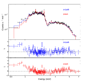
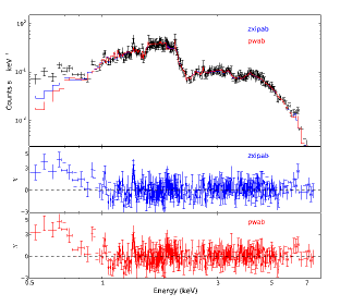
Figure 2: Chandra/HETG spectra of NY Lup (left panel) and V1223 Sgr (right panel) overlaid with the complex absorption model zxipab (blue) and pwab (red).The second and third panels (note the Y scale changes between the two for NY Lup) of the plots are residuals to the zxipab and pwab models respectively.

2.2 Photo-ionized emission lines

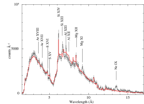
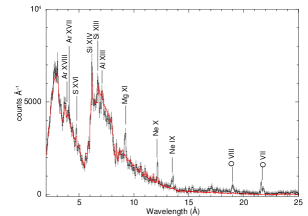
Figure 3: Chandra MEG summed first order spectra of NY Lup (left panel) and V1223 Sgr (right panel), along with various emission lines. The red line is the best-fit spectral model using an ionized absorber model zxipab and cooling flow model mkcflow, along with a reflection component reflect. Data show excess flux for Si XIII, Mg XI and Ne IX lines for NY Lup and Mg XI, Ne IX and OVII lines for V1223 Sgr

.

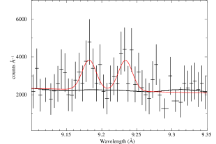
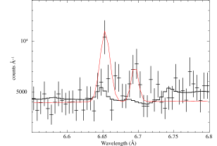
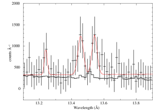
Figure 4: Chandra MEG summed first order spectra of NY Lup showing the presence of He like triplets of Mg XI (left panel), Si XIII (right panel) and Ne IX (bottom panel). The gaussian fits to the emission lines are shown in red and the predictions of the line strengths with mkcflow model is shown in black line. The spectra is binned for clarity

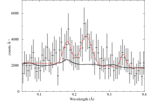
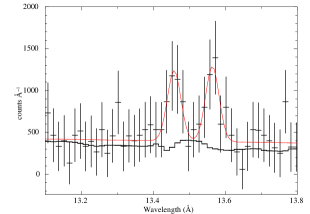
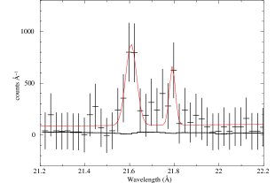
Figure 5: Chandra MEG summed first order spectra of V1223 Sgr showing the presence of He like triplets of Mg XI (left panel), Ne IX (middle panel) and O VII (right panel). The gaussian fits to the emission lines are shown in red and the predictions of the line strengths with mkcflow model is shown in black line. The spectra is binned for clarity

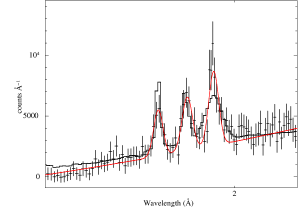
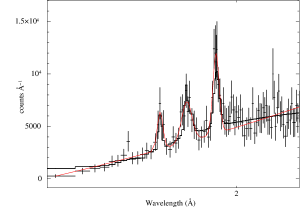
Figure 6: Chandra HEG summed first order spectra of NY Lup (left panel) and V1223 Sgr (right panel) showing the presence of neutral, He like (Fe XXV) and H like Fe K$\alpha$ lines (Fe XXVI). The gaussian fits to the emission lines are shown in red and the predictions of the line strengths with mkcflow model plus a gaussian line to model the Fe K$\alpha$ line, is shown in black line. The spectra is binned for clarity

Figure 3 shows the MEG summed first order spectra of NY Lup and V1223 Sgr, displaying the emission lines along with their predictions from the cooling flow mkcflow model. We see the presence of H and He like ions emission lines from Ne, Mg, Al, Si, Ar and S in the MEG spectra of NY Lup and V 1223 Sgr. We also see emission lines corresponding to He and He like ion of O in V1223 Sgr, which are not seen in NY Lup, most likely due to the decreased low energy effective area of ACIS in the 2016 Chandra HETG observation of NY Lup. We find the model predictions of the line strengths from the mkcflow model describe the fluxes of most of the emission lines, except for certain He like triplets of Si, Mg XI, Ne IX and O VII. Figure 4 shows the MEG first order summed spectra of NY Lup around Mg XI, Si XIII and Ne IX emission lines. We can resolve He like triplet lines of Ne IX emission lines, which are fitted with three gaussian lines in the plot. For Mg XI and Si XIII, we can only resolve two lines out of the expected He like triplets, due to low statistics of the third line. These are fitted with two gaussian lines in the plot. Figure 5 shows the MEG first order summed spectra of V1223 Sgr around Mg XI, Ne IX and O VII emission lines. We can resolve the He like triplet lines of Mg XI and are fitted with three gaussian lines in the plot. For Ne IX and O VII, we can only resolve two lines out of the expected He like triplets, due to low statistics of the third line. These are fitted with two gaussian lines in the plot. In all these plots, the primary emission is fitted by a first order polynomial plus the gaussians for the emission lines. To estimate the excess X-ray fluxes of these emission lines which are resolved into double or triple lines, we fit them with a gaussian line and estimate their excess flux over the predictions from the mkcflow model. Table 3 and 4 shows the excess X-ray flux of these photo-ionized lines over their flux predictions by the mkcflow model. The errors are calculated at 90% of the confidence limit on the normalisation of the gaussian lines used to model these emission lines and propagated to account for the errors on the fluxes.

Figure 6 shows the HEG summed first order spectra around Fe lines of NY Lup and V1223 Sgr, with the emission lines corresponding to neutral Fe (Fe K$\alpha$), He like Fe (Fe XXV) and H like Fe (Fe XXVI). The primary emission is modelled with the cooling flow model mkcflow and a gaussian line for Fe K$\alpha$.

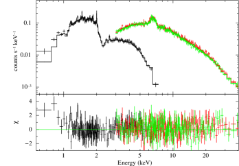
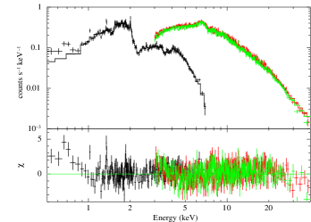
Figure 7: Chandra/HETG (black) + NuSTAR (FPMA: red and FPMB: green) spectral fit to NY Lup (left panel) and V1223 Sgr (right panel) using the model defined in Section 2.1 with the ionized absorber model zxipab (right panel), along with ratio of the data to the model. The Chandra/HETG and NuSTAR spectra are rebinned for clarity.

Our complete fitting results using a spectral model with an ionized absorber model zxipab, cooling flow model mkcflow, reflection component reflect and gaussian emission lines for Fe K$\alpha$ line and the emission lines described in Section 2.2 whose observed fluxes do not match the cooling flow model predictions, are shown in Figure 7 along with their residuals for NY Lup and V1223 Sgr.

3 Discussion

Previous study by Mukai et al. (2003) classified the Chandra/HETG spectra of 7 CVs into two groups based on their X-ray spectra. EX Hya, V603 Aql, U Gem and SS Cyg were classified as cooling-flow type since their X-ray spectra are described well using the mkcflow model, which was originally developed to model the cooling flows in clusters of galaxies (Mushotzky & Szymkowiak, 1988). In these four CVs, the cooling flow model provides a good explanation for the continuum shape as well as the strong H and He like emission lines of O, Ne, Mg, Al, Si, S and entire Fe L complex (Figure 1 in Mukai et al. 2003). On the other hand, in the three other CVs studied by Mukai et al. (2003) (V1223 Sgr, AO Psc, and GK Per), the continuum is much harder than what the cooling flow model mkcflow predicts; the details of the observed emission lines are also different from mkcflow predictions. Specifically, the Fe L lines are weaker than expected, and the ratio of fluxes of of He-like ions to those of H-like ions are higher than predicted. These discrepancy led Mukai et al. (2003) to explain the entire Chandra/HETG spectra of these three CVs using a photo-ionization model.

However, there are several issues with this interpretation. First, it is difficult to imagine a situation where the modest luminosity (of order 10³⁴ erg/s) of these CVs can nevertheless produce H-like and He-like lines of Fe through photo-ionization. Second, the hard power-law continuum of Mukai et al. (2003) was an ad-hoc assumption, incompatible with the standard understanding that the strong shock is the primary source of emission in IPs. Various studies (including Mukai et al. 2015) focusing on the harder end of the X-ray spectra of these ‘photo-ionized’ CVs have already demonstrated that they can be modelled by a cooling flow spectra modified by a complex distribution of absorbers in the pre-shock region. Such models attribute the H-like and He-like emission lines of Fe to the collisionally-excited, multi-temperature, post-shock plasma. They explain the hard power-law like continuum as that of multi-temperature bremsstrahlung emission hardened by the complex absorber (see Appendix for an analytical understanding of this).

Given the specific accretion rate (accretion rate per unit surface area) $\dot{m}$, and assuming a shock very close to the stellar surface, we can estimate both the density of the pre-shock flow and the photon flux through this region. The pre-shock density is $\dot{m}$ divided by the free-fall velocity. For a 0.8 M_⊙ white dwarf, the free-fall velocity is 5.5$\times 10^{8}$ cm s^-1 and the pre-shock density is 1.82$\times 10^{-9}$ $\dot{m}$ g cm^-3, or number density of 1.8$\times 10^{15}$ $\dot{m}$ cm^-3. We can obtain the accretion luminosity per unit area by multiplying $\dot{m}$ with gravitational potential (GM/R) of the white dwarf. For a 0.8 M_⊙ white dwarf, the luminosity per unit area is 1.5$\times 10^{17}$ $\dot{m}$ erg s^-1, of which half will be radiated downward and converted into soft photons, so the hard X-ray luminosity is 7.5$\times 10^{16}$ $\dot{m}$ erg s^-1. The ionization parameter, $\xi=L/nr^{2}$, generalized for a cloud adjacent to an extended source of ionizing radiation, is independent of $\dot{m}$ and $\sim$40 in the 0.8 M_⊙ immediately above the shock. However, the actual value will be lower due to geometrical dilution (both due to finite shock height, and finite distance above the shock front). We therefore expect the immediate pre-shock flow to be modestly, but measurably ionized. This expectation is confirmed by the presence of photo-ionized emission lines and warm absorption features, seen in Figure 2 and 3. This justifies our decision to develop a model for ionized distribution of absorbers in the pre-shock region, zxipab (see Appendix for the details of the model).

Figure 1 shows the model prediction of the complex absorption models zxipab and pwab at lower energies. There is a significant deviation between the prediction of the two models at energies $\leq$ 0.8 keV. The ionized absorber model zxipab shows the presence of sharp discontinuity due to OVII edge at $\sim$ 0.9 keV, which is also seen in the Chandra/HETG spectrum of V1223 Sgr (Figure 2). Due to the decreased effective area of Chandra/HETG, this is not as obvious for NY Lup. When we see the X-rays escaping through the pre-shock region, it shows warm absorber features. This pre-shock region is likely the origin of the photo-ionized emission lines as well. Future missions like XRISM would be important in detecting the presence of warm absorber like absorption lines from these CVs.

The Chandra/HETG spectra of NY Lup and V1223 Sgr in Figure 3 shows the presence of emission lines from H and He like ions of Ne, Mg, Al, Si, S, Fe. Many of these lines are from the collisionally excited plasma, since the cooling flow model mkcflow predict the line fluxes accurately. However the line predictions of the cooling flow model fails to account for the He like lines of some medium Z elements. These are the lines that we ascribe to photo-ionization. He-like triplets have a good diagnostic capability, and line ratios can be used as an independent test of the line origin (collisional vs photo-ionized) (Porquet & Dubau, 2000; Porquet et al., 2001). However, Mukai et al. (2003) argued that this diagnostic is not appropriate for CVs, because the radial velocity gradient of thousands of km/s can result in all the lines remaining completely unsaturated at all ionic column densities. This leaves the plasma in photo-excitation dominated regime, in which the resonance lines are stronger than in photo-ionization dominated regime (Kinkhabwala et al., 2002). Also, resonant scattering may have an important effect on the line ratios in CVs (Terada et al., 2004). Moreover, Chandra HETG observations of CVs are far too underexposed to be able to use such diagnostics (Schlegel et al., 2014). For all these reasons, existing data cannot be used to derive a definitive origin of the lines that the cooling flow models cannot account for. The neutral Fe K$\alpha$ originates both from the white dwarf surface and pre-shock flow (Ezuka & Ishida, 1999).

The NuSTAR observations of NY Lup and V1223 Sgr show the presence of a Compton hump in its hard X-ray spectra and an energy dependent spin modulations with an amplitude of $\leq 10\%$ (Mukai et al., 2015). Both these findings point to the fact that the shock is close to the white dwarf surface (a shock height of 0.05 R_wd for V1223 Sgr and a negligible shock height for NY Lup; see Mukai et al. 2015) resulting in strong Compton reflection off the white dwarf surface. This also results in strong complex absorption, and significant degree of ionization of the pre-shock flow. All these are consequences of high specific accretion rate $\dot{m}$. In contrast, EX Hya has a lower $\dot{m}$ and hence tall shocks ($\sim$ R_wd; where $R_{wd}$ is radius of the white dwarf ) allowing X-rays to escape the post-shock region by travelling through the sides. Hence there is an absence of complex absorption or reflection in its X-ray spectra (Luna et al., 2018).

Figure 7 shows the broadband fit of the Chandra/HETG and NuSTAR spectra of NY Lup and V1223 Sgr in energy range of 0.5–40 keV. The spectral model used for this broadband fit consists of the ionized absorber model zxipab, cooling flow model mkcflow, reflection component reflect and gaussian lines to model the emission from Fe K$\alpha$ and photo-ionized lines. The presence of every model component is physically motivated. We therefore conclude that this is superior to the artificial model of Mukai et al. (2003).

Given that the shock is close to the white dwarf surface in many magnetic CVs, roughly half the radiation will intercept the stellar surface and heat it up. For a 0.8 M_⊙ white dwarf accreting at $\dot{m}$ of 1.0 g s^-1cm^-2, kT$\sim$20 eV blackbody is expected. While just such a component is prominent in the majority of polars, no such component was seen in IPs until Haberl & Motch (1995) discovered three “soft IPs” with such a component. Haberl et al. (2002) inferred the presence of such a component in NY Lup, with an estimated temperature of 86 eV. Since then, the presence of the soft component has been inferred in quite a few IPs (Evans & Hellier, 2007; Anzolin et al., 2008). However, the high inferred blackbody temperatures in several IPs, including NY Lup, presents a potentially serious problem, because the luminosity per unit area is so high that some may violate the Eddington limit, and is likely to violate the atmospheric limit (Williams et al., 1987). However previous claims of a soft component is based on the spectral fits without ionized complex absorbers or photo-ionized emission lines. In Figure 2, we find residuals at lower energies while fitting the Chandra/HETG spectra with complex absorber models; the residuals are lower for the zxipab model compared to the pwab model. However there are uncertainties related to the interstellar absorption related to its estimation using Chandra/HETG data and the instrumental calibrations issues related to ACIS degradation, which could be related to these soft excess. We attempted to fit these soft excess with a blackbody component. However, this did not result in a statistically significant improvement of fit quality, suggesting the soft excess may not have the right shape to be explained with a blackbody component. The temperature we derive, which is unphysical for these systems, is therefore also a suspect. We tentatively conclude that, when the correct spectral model (including ionized complex absorber and photo-ionized lines), the need for the blackbody may disappear, or the blackbody temperature may not be as hot as previously claimed.

4 Summary

We have developed a new, ionized version (zxipab) of the complex absorber model pwab, and applied it, along with the cooling flow model mkcflow, the reflection model reflect, and Gaussian emission lines, to Chandra/HETG and NuSTAR spectra of two IPs, NY Lup and V1223 Sgr. Our findings are as follows:

• The ionized version provides a better, although still not a complete explanation of the spectra below 1 keV than the neutral version.

• We attribute the excess emission lines that cannot be explained with the absorbed cooling flow as due to photo-ionized emission from the immediate pre-shock flow, the same region that is responsible for the complex absorption.

• Once both these are taken into account, the soft blackbody component that was previously claimed for NY Lup may not be necessary. The previously claimed parameters of the blackbody component certainly are subject to revision.

Appendix: Complex Ionized Absorber Model, zxipab

Analytical Considerations

We take equation (1) of Done & Magdziarz (1998) as our starting point.

$$S(E)=S_{\rm int}(E)A\int_{N_{H,min}}^{N_{H,max}}N_{H}^{\beta}\exp{(-N_{H}\sigma(E))}dN_{H}$$ (1)

This assumes a power-law distribution of covering fraction as a function of the absorbing column, i.e., $C_{f}(N_{H})\propto N_{H}^{\beta}$ and $A$ is the normalization such that $\int_{N_{H,min}}^{N_{H,max}}C_{f}(N_{H})=1.0$. The effect of such an absorber is markedly different from that of a simple absorber. The latter results in an exponential decline in transmission at low energies, which is often the handle that allows one to fit for N_H. The combination of a simple absorber (e.g., from the inter-stellar medium) and a partial covering absorber produces two such exponential cut-offs, with a region in energy where the observed spectrum is dominated by the unabsorbed component. The effect of of pwab is more power-law like (see, e.g., Figure 9 of Mukai 2017).

This can be understood using the following considerations. By substituting $u=N_{H}\sigma(E)$, we obtain

$$T(E)\propto\sigma(E)^{-\beta-1}\int_{u_{min}}^{u_{max}}u^{\beta}\exp{(-u)}du$$ (2)

for the transmission $T(E)$. The integral can be expressed in terms of incomplete gamma function $P(a,x)=1/\Gamma(a)\int_{0}^{x}t^{a-1}\exp{(-t)}dt$ so that

$$T(E)\propto\sigma(E)^{-\beta-1}[P(\beta+1,u_{max})-P(\beta+1,u_{min})]$$ (3)

The properties of the incomplete gamma function is well known: for a small positive value of $a$, it rises quickly from 0 to $\sim$1. If $N_{H,min}$ is sufficiently small and $N_{H,max}$ is sufficiently large, there is a range of $E$ such that $P(\beta+1,u_{max})\sim 1$ and $P(\beta+1,u_{min})\sim 0$, so that

$$T(E)\propto\sigma(E)^{-\beta-1}$$ (4)

At the same time, $\sigma(E)$ itself can be approximated by a power law of $E$. For example,

$$\sigma(E)=2.242\times 10^{-22}(E/1keV)^{-8/3}cm^{-2}$$ (5)

is a good approximation of the photoelectric cross section of Morrison & McCammon (1983) between O and Fe edges. Thus, the power-law distribution of covering fraction can lead to a power-law like, rather than exponential, low-energy cut-off.

$\sigma$ has discontinuities at the major edges. The neutral and ionized versions are different in the positions and the depth of the discontinuities. In particular, if all K shell electrons of lower Z elements are ionized, $\sigma$ becomes close to 0 at low energies. In such a situation, the use of zxipab is necessary, while a combination of pwab and an edge would provide a poor approximation for energies where $\sigma\sim 0$.

The implementation and current limitations

The neutral version of the model, pwab, numerically integrates the neutral absorber model, wabs (Morrison & McCammon, 1983). For zxipab, we replace the call to wabs model with a pre-calculated grid of XSTAR photoionization model that was originally used for the partial covering warm absorber model, zxipcf (Reeves et al., 2008). Model parameters are the minimum and the maximum N_H, power law index for covering fraction (from pwab), the ionization parameter log($\xi$), and the redshift of the absorber.

As with pwab, zxipab approximates the true differential covering fraction distribution using a power law. This is an intrinsic limitation of the model. A more realistic model of pre-shock flow absorption in magnetic CVs should replace the power law with a more realistic function, although this could rapidly expand the number of free parameters to describe, e.g., the shape of the footpoint of the accretion curtain. Also, zxipab assumes a single log($\xi$) for the absorber, whereas a realistic absorber model would also include a distribution of log($\xi$) as a function of distance from the shock front. Finally, zxipab assumes the absorber with solar abundances, which is not guaranteed to hold for all magnetic CVs, particularly for the nitrogen abundance (see, e.g., the case of V2731 Oph: Lopes de Oliveira & Mukai 2019).

zxipab is available as a new model in XSPEC through this website.

References

- Anzolin et al. (2008) Anzolin, G., de Martino, D., Bonnet-Bidaud, J. M., et al. 2008, A&A, 489, 1243
- Arnaud (1996) Arnaud, K. A. 1996, in Astronomical Society of the Pacific Conference Series, Vol. 101, Astronomical Data Analysis Software and Systems V, ed. G. H. Jacoby & J. Barnes, 17
- Asplund et al. (2009) Asplund, M., Grevesse, N., Sauval, A. J., & Scott, P. 2009, ARA&A, 47, 481
- Beuermann et al. (2004) Beuermann, K., Harrison, T. E., McArthur, B. E., Benedict, G. F., & Gänsicke, B. T. 2004, A&A, 419, 291
- Canizares et al. (2005) Canizares, C. R., Davis, J. E., Dewey, D., et al. 2005, PASP, 117, 1144
- de Martino et al. (2008) de Martino, D., Matt, G., Mukai, K., et al. 2008, A&A, 481, 149
- Done & Magdziarz (1998) Done, C., & Magdziarz, P. 1998, MNRAS, 298, 737
- Done et al. (1995) Done, C., Osborne, J. P., & Beardmore, A. P. 1995, MNRAS, 276, 483
- Evans & Hellier (2007) Evans, P. A., & Hellier, C. 2007, ApJ, 663, 1277
- Ezuka & Ishida (1999) Ezuka, H., & Ishida, M. 1999, ApJS, 120, 277
- Fabian (1994) Fabian, A. C. 1994, ARA&A, 32, 277
- Fabian & Nulsen (1977) Fabian, A. C., & Nulsen, P. E. J. 1977, MNRAS, 180, 479
- Fruscione et al. (2006) Fruscione, A., McDowell, J. C., Allen, G. E., et al. 2006, in Society of Photo-Optical Instrumentation Engineers (SPIE) Conference Series, Vol. 6270, Society of Photo-Optical Instrumentation Engineers (SPIE) Conference Series, ed. D. R. Silva & R. E. Doxsey, 62701V
- Haberl & Motch (1995) Haberl, F., & Motch, C. 1995, A&A, 297, L37
- Haberl et al. (2002) Haberl, F., Motch, C., & Zickgraf, F. J. 2002, A&A, 387, 201
- Harrison et al. (2013) Harrison, F. A., Craig, W. W., Christensen, F. E., et al. 2013, ApJ, 770, 103
- Hayashi et al. (2021) Hayashi, T., Kitaguchi, T., & Ishida, M. 2021, MNRAS, 504, 3651
- Kinkhabwala et al. (2002) Kinkhabwala, A., Sako, M., Behar, E., et al. 2002, ApJ, 575, 732
- Lopes de Oliveira & Mukai (2019) Lopes de Oliveira, R., & Mukai, K. 2019, ApJ, 880, 128
- Luna et al. (2018) Luna, G. J. M., Mukai, K., Orio, M., & Zemko, P. 2018, ApJ, 852, L8
- Morrison & McCammon (1983) Morrison, R., & McCammon, D. 1983, ApJ, 270, 119
- Mukai (2017) Mukai, K. 2017, PASP, 129, 062001
- Mukai et al. (2003) Mukai, K., Kinkhabwala, A., Peterson, J. R., Kahn, S. M., & Paerels, F. 2003, ApJ, 586, L77
- Mukai et al. (2015) Mukai, K., Rana, V., Bernardini, F., & de Martino, D. 2015, ApJ, 807, L30
- Mushotzky & Szymkowiak (1988) Mushotzky, R. F., & Szymkowiak, A. E. 1988, in NATO Advanced Science Institutes (ASI) Series C, Vol. 229, NATO Advanced Science Institutes (ASI) Series C, ed. A. C. Fabian, 53
- Norton & Watson (1989) Norton, A. J., & Watson, M. G. 1989, MNRAS, 237, 853
- Peterson et al. (2003) Peterson, J. R., Kahn, S. M., Paerels, F. B. S., et al. 2003, ApJ, 590, 207
- Porquet & Dubau (2000) Porquet, D., & Dubau, J. 2000, A&AS, 143, 495
- Porquet et al. (2001) Porquet, D., Mewe, R., Dubau, J., Raassen, A. J. J., & Kaastra, J. S. 2001, A&A, 376, 1113
- Reeves et al. (2008) Reeves, J., Done, C., Pounds, K., et al. 2008, MNRAS, 385, L108
- Schlegel et al. (2014) Schlegel, E. M., Shipley, H. V., Rana, V. R., Barrett, P. E., & Singh, K. P. 2014, ApJ, 797, 38
- Shaw et al. (2018) Shaw, A. W., Heinke, C. O., Mukai, K., et al. 2018, MNRAS, 476, 554
- Terada et al. (2004) Terada, Y., Ishida, M., & Makishima, K. 2004, PASJ, 56, 533
- Williams et al. (1987) Williams, G. A., King, A. R., & Brooker, J. R. E. 1987, MNRAS, 226, 725