Quantum particle on a surface: Catenary surface and paraboloid of revolution

Abstract

We revisit the Schrödinger equation of a quantum particle that is confined on a curved surface. Inspired by the novel work of R. C. T. da Costa [1] we find the field equation in a more convenient notation. The contribution of the principal curvatures in the effective binding potential on the surface is emphasized. Furthermore, using the so-called Monge-Gauge we construct the approximate Schrödinger equation for a flat surface with small fluctuations. Finally, the resulting Schrödinger equation is solved for some specific surfaces. In particular, we give exact solutions for a particle confined on a Catenary surface and a paraboloid of revolution.

I Introduction

Nowadays, studying the propagation of quantum particles on curved surfaces became of interest in different areas of experimental and theoretical physics. Graphene with only one atom thickness is one of such 2-dimensional surface-like materials Graphene . Furthermore, another surface-like material is the so-called carbon nanotube CNT with stronger $sp^{2}$ bonds which make it one of the best thermal conductors CNT2 . Another important 2D material that has been the subject of intensive research both experimentally and theoretically is Phosphorene, a monolayer of black phosphorus PHOS (see also the references therein). It is a 2D semiconductor material with an anisotropic orthorhombic structure and high optical and UV absorption. To this list of 2-dimensional materials we would like to add the so-called fluid lipid membranes FLM which has shown a growing interest among physicists, mathematicians, and biologists.

Concerning these highly important lower-dimensional materials, and the quantum phenomenon on these surfaces, one has to create/construct an induced lower-dimensional quantum mechanics which may be applied to such 2-dimensional materials. Such a formalism has been introduced long time ago in 2dQ and 2dQ2 . However, the recent work of Ferrari and Cuoghi PRL1 , proves that the story has not been over yet. To summarize the difference between these three works, one observes the following. In 2dQ , the action principle has been considered directly in n-dimensional curved space. Hence, considering $n=2$ one gets the quantum on a curved surface. In 2dQ2 , using the differential geometrical properties of the curved surface, the Schrödinger equation in 3-dimensional Euclidean space has been reduced to the Schrödinger equation on the surface. In PRL1 , the formalism of 2dQ2 has been extended by including the electric and magnetic fields. Following these seminal works, there have been significant improvements in the quantum systems in the two-dimensional curved surfaces as well as on curves. In this line, we may refer to Flipe where the effects of the geometry, as well as magnetic field on the electronic transport properties of metallic nanotubes, have been numerically investigated. In Jose , an electron confined on a torus under the influence of external electric and magnetic fields has been numerically studied. In Silva the authors studied the an electron on a catenoid surface. Oliveira et al in Oliveria solved the Schrödinger equation on a sphere under non-central potential and Schmidt in Schmidt and Schmidt2 introduced exact solutions of Schrödinger equation for a charged particle confined on a sphere, on a cylinder and on a torus while is imposed with uniform electric and magnetic fields. Furthermore, electrons confined on a rotating sphere in the presence of a magnetic field have been considered by Lima et al in Lima , and the effects of the rotation were compared with the effects of the magnetic fields. The application of this formalism has not been limited only to these works, for instance, we refer to Application for further reading.

I.1 Our motivation

We observed that most of the papers published recently are based on the effective Schrödinger equation derived in 2dQ2 , particularly Eq. (14). In driving this equation, R. C. T. da Costa used a kind of unfamiliar notation to our new generation of young physicists. For instance, while these days we are very careful on distinguishing between contravariant and covariant vectors especially when the contraction of tensors is in the subject, in 2dQ2 , it was only a matter of notation. Therefore, many steps in finding the effective Schrödinger equation in 2dQ2 are unfamiliar. The aim of this paper is first to construct a full detailed calculation with modern - so to say - notation toward the effective Schrödinger equation. We should add that there are some other works that looked at this issue from another perspective. For instance, a very general, as well as an interesting approach to the constraint motion of a quantum particle in n-dimensional Euclidian space, has been studied by P.C. Schuster and R.L. Jaffe in Schuster . In addition, the applications of some specific parametrization such as Monge parametrization seem to be missing in the literature. Since for surfaces such as graphene, the small deviation from a flat surface may be of interest the application of Monge gauge becomes important. Hence, we study the quantum particle under Monge parametrization and for small deviation deviations, we present the simplified approximate effective Schrödinger equation. Finally, the exact solutions of the effective Schrödinger equation for quantum particles confined on some important curved surfaces such as Catenoid and paraboloid of revolution are missing. Therefore, we investigate the possible exact solutions for these two cases.

II Schrödinger equation on a curved surface

We consider a quantum particle of mass $m$ confined on a differentiable surface $S$ in the three-dimensional Euclidean space. We also adopt a local two-dimensional coordinate system $\left\{u^{1},u^{2}\right\}$ on the surface and a mapping $\mathbf{r:}=\mathbf{r}\left(u^{1},u^{2}\right)$ which assigns any point on the surface to a point on the three-dimensional space, i.e.,

$$\mathbf{r:}=\mathbf{r}\left(u^{1},u^{2}\right)=\left(x^{1}\left(u^{1},u^{2}\right),x^{2}\left(u^{1},u^{2}\right),x^{3}\left(u^{1},u^{2}\right)\right).$$ (1)

Herein, the position vector $\mathbf{r}=\left(x^{1},x^{2},x^{3}\right)$ represents a point on the surface while a point in the neighborhood of the surface can be described using an additional coordinate i.e., $u^{3}$ in the direction normal to the surface (see Fig. 1).

Figure 1:

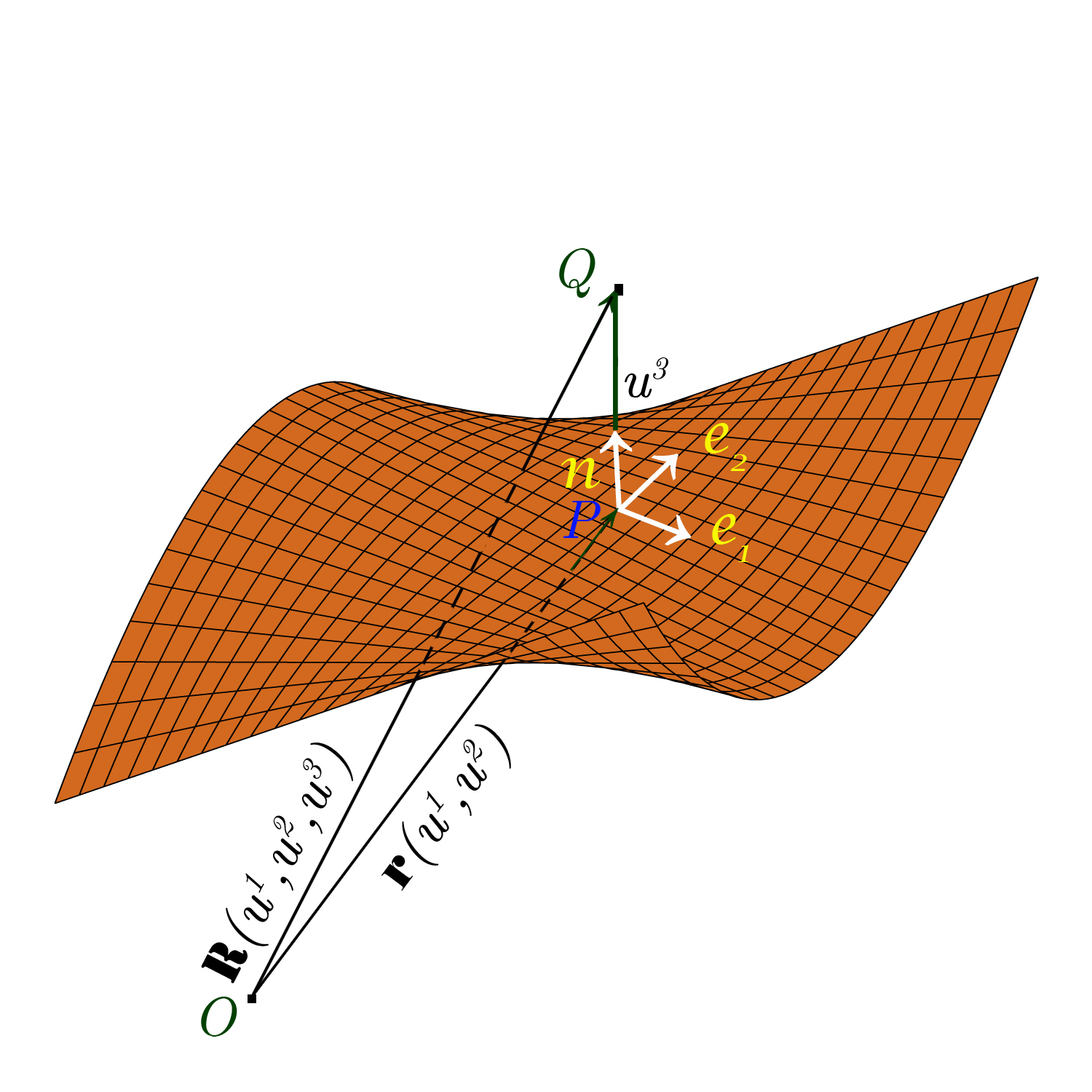
The curvilinear coordinate system addressing the surface and the ambience.

Hence, one writes

$$\mathbf{R}\left(u^{1},u^{2},u^{3}\right)=\mathbf{r}\left(u^{1},u^{2}\right)+u^{3}\mathbf{n.}$$ (2)

We note that the tangent vectors

$$\mathbf{e}_{a}=\frac{\partial\mathbf{r}}{\partial u^{a}}=\mathbf{\partial}_{a}\mathbf{r}$$ (3)

with $a=1,2,$ make a local $2$-dimensional coordinate system that spans the tangent surface to $S$ at any point $P$ on $S$ where $\mathbf{e}_{a}$ are determined. Furthermore, the three-dimensional coordinate system consists of two tangent vectors $\mathbf{e}_{a}$ and the unit normal $\mathbf{n}$ make a local 3-dimensional coordinate system which describes the space surrounding the surface $S$ such that

$$\mathbf{n}=\frac{\mathbf{e}_{1}\times\mathbf{e}_{2}}{\left|\mathbf{e}_{1}\times\mathbf{e}_{2}\right|}.$$ (4)

We add that, in general, $\mathbf{e}_{a}$ are neither unit vectors nor orthogonal, however, $\mathbf{n}$ is unit vector and normal to $\mathbf{e}_{a}.$ Furthermore, the $3$-dimensional coordinate system as well as the two dimensional one are curvilinear, and based on the tangent vectors $\mathbf{e}_{a}$ and the normal vector $\mathbf{n}$, one constructs the metric tensor of the space and the surface as defined by

$$g_{\mu\nu}=\frac{\partial\mathbf{R}}{\partial u^{\mu}}.\frac{\partial\mathbf{R}}{\partial u^{\nu}}$$ (5)

and

$$h_{ab}=\frac{\partial\mathbf{r}}{\partial u^{a}}.\frac{\partial\mathbf{r}}{\partial u^{b}},$$ (6)

respectively, in which $\mu,\nu=1,2,3$ and $a,b=1,2.$ Let’s add that $h_{ab}$ is called the first fundamental form of the surface $S$ which is an intrinsic geometrical property of the surface. In addition to the first fundamental form, there exist the second fundamental form of the surface which is an extrinsic property of the surface and is defined by

$$k_{ab}:=\mathbf{e}_{a}.\partial_{b}\mathbf{n}$$ (7)

which due to the fact that $\mathbf{e}_{a}.\mathbf{n}=0$, it is also equal to

$$k_{ab}=-\mathbf{n}.\partial_{ab}\mathbf{r.}$$ (8)

The second fundamental form $k_{ab}$ is also called the extrinsic curvature tensor because it is defined in terms of the normal vector $\mathbf{n}$ which is an indication of the embedding of the surface in a higher-dimensional space/ambiance..

Coming back to the metric tensor of the space surrounding the surface one writes

$$g_{ab}=\frac{\partial\mathbf{R}}{\partial u^{a}}.\frac{\partial\mathbf{R}}{\partial u^{b}}=\left(\mathbf{e}_{a}+u^{3}\partial_{a}\mathbf{n}\right).\left(\mathbf{e}_{b}+u^{3}\partial_{b}\mathbf{n}\right),$$ (9)

$$g_{a3}=g_{3a}=\left(\mathbf{e}_{a}+u^{3}\partial_{a}\mathbf{n}\right).\mathbf{n}$$ (10)

and

$$g_{33}=\mathbf{n}.\mathbf{n}=1.$$ (11)

To calculate $g_{ab},$ $g_{a3}$ and $g_{3a}$ we apply the so-called equation of Weingarten which states

$$\partial_{a}\mathbf{n}=k_{a}^{b}\mathbf{e}_{b}$$ (12)

in which $k_{a}^{b}=h^{bc}k_{ac}$ is the mixed form of the extrinsic curvature tensor and $h^{bc}$ is the inverse of the metric tensor $h_{bc}$ such that $h_{ac}h^{cb}=\delta_{a}^{b}.$ Considering (12) in (9) one finds

$$g_{ab}=\mathbf{e}_{a}.\mathbf{e}_{b}+u^{3}\partial_{a}\mathbf{n.e}_{b}+u^{3}\mathbf{e}_{a}.\partial_{b}\mathbf{n+}\left(u^{3}\right)^{2}\partial_{a}\mathbf{n.}\partial_{b}\mathbf{n}$$ (13)

or simply

$$g_{ab}=h_{ab}+u^{3}k_{a}^{c}h_{cb}+u^{3}k_{b}^{c}h_{ac}\mathbf{+}\left(u^{3}\right)^{2}k_{a}^{c}k_{b}^{d}h_{cd}$$ (14)

and $g_{a3}=g_{3a}=0.$ Having the first and the second fundamental forms symmetric, we obtain

$$g_{ab}=h_{ab}+2u^{3}k_{a}^{c}h_{cb}\mathbf{+}\left(u^{3}\right)^{2}k_{a}^{c}k_{b}^{d}h_{cd}.$$ (15)

Using the so-called Laplace-Beltrami operator the Schrödinger equation of a particle in the space spanned with $g_{\mu\nu}$ is given by

$$-\frac{\hslash^{2}}{2m}\frac{1}{\sqrt{g}}\partial_{\mu}\left(\sqrt{g}g^{\mu\nu}\partial_{\nu}\right)\psi\left(u^{\alpha},t\right)+V_{0}\tilde{\delta}\left(u^{3}\right)\psi\left(u^{\alpha},t\right)=i\hslash\frac{\partial}{\partial t}\psi\left(u^{\alpha},t\right)$$ (16)

in which $V_{0}\tilde{\delta}\left(u^{3}\right)$ is a potential which confines the particle on the surface $S$ and $\tilde{\delta}\left(u^{3}\right)$ is an anti-Dirac delta function such that

$$\tilde{\delta}\left(u^{3}\right)=\left\{\begin{array}[]{cc}0&u^{3}=0\\ \infty&u^{3}\neq 0\end{array}\right..$$ (17)

To simplify (16), one needs to calculate $g=\det g_{\mu\nu}$, i.e.

$$g=\det\left[\begin{array}[]{ccc}g_{11}&g_{12}&0\\ g_{21}&g_{22}&0\\ 0&0&1\end{array}\right]=\det\left[\begin{array}[]{cc}g_{11}&g_{12}\\ g_{21}&g_{22}\end{array}\right]=g_{11}g_{22}-\left(g_{12}\right)^{2}$$ (18)

where

$$g_{11}=h_{11}+2u^{3}k_{1}^{c}h_{c1}\mathbf{+}\left(u^{3}\right)^{2}k_{1}^{c}k_{1}^{d}h_{cd}$$ (19)

$$g_{22}=h_{22}+2u^{3}k_{2}^{c}h_{c2}\mathbf{+}\left(u^{3}\right)^{2}k_{2}^{c}k_{2}^{d}h_{cd}$$ (20)

and

$$g_{12}=g_{21}=h_{12}+2u^{3}k_{1}^{c}h_{c2}\mathbf{+}\left(u^{3}\right)^{2}k_{1}^{c}k_{2}^{d}h_{cd}$$ (21)

upon which

$$g=\left(h_{11}+2u^{3}k_{1}^{c}h_{c1}\mathbf{+}\left(u^{3}\right)^{2}k_{1}^{c}k_{1}^{d}h_{cd}\right)\left(h_{22}+2u^{3}k_{2}^{a}h_{a2}\mathbf{+}\left(u^{3}\right)^{2}k_{2}^{a}k_{2}^{b}h_{ab}\right)-\\ \left(h_{12}+2u^{3}k_{1}^{c}h_{c2}\mathbf{+}\left(u^{3}\right)^{2}k_{1}^{c}k_{2}^{d}h_{cd}\right)\left(h_{21}+2u^{3}k_{2}^{a}h_{a1}\mathbf{+}\left(u^{3}\right)^{2}k_{2}^{a}k_{1}^{b}h_{ab}\right).$$ (22)

After some manipulation, the latter equation reduces to

$$g=\left(h_{22}h_{11}-h_{12}^{2}\right)\left(1+u^{3}\left(k_{1}^{1}+k_{2}^{2}\right)+\left(u^{3}\right)^{2}\left(k_{1}^{1}k_{2}^{2}-k_{1}^{2}k_{2}^{1}\right)\right)^{2}.$$ (23)

We remember that the trace and the determinant of the extrinsic curvature tensor are invariant under the coordinate transformation. Therefore, although $k_{a}^{b}$ is not diagonal and consequently $k_{1}^{1}$ and $k_{2}^{2}$ are not the principal curvatures, but $k_{1}^{1}+k_{2}^{2}=Tr\left(k_{a}^{b}\right)=$ $\tilde{k}_{1}^{1}+\tilde{k}_{2}^{2}$ and $k_{1}^{1}k_{2}^{2}-k_{1}^{2}k_{2}^{1}=\det\left(k_{a}^{b}\right)=\tilde{k}_{1}^{1}\check{k}_{2}^{2}$ in which $\tilde{k}_{1}^{1}$ and $\tilde{k}_{2}^{2}$ are the principal curvatures of the surface. Considering the above facts one writes

$$g=h\left(1+u^{3}\left(\tilde{k}_{1}^{1}+\tilde{k}_{2}^{2}\right)+\left(u^{3}\right)^{2}\tilde{k}_{1}^{1}\check{k}_{2}^{2}\right)^{2}$$ (24)

where

$$h=h_{22}h_{11}-h_{12}^{2}=\det\left(h_{ab}\right).$$ (25)

We also recall the definition of the Gaussian and total curvatures in terms of the principal curvatures which are defined as

$$K_{G}=\tilde{k}_{1}^{1}\check{k}_{2}^{2}$$ (26)

and

$$K=\tilde{k}_{1}^{1}+\tilde{k}_{2}^{2},$$ (27)

respectively, which simplifies (24) as

$$g=h\left(1+u^{3}K+\left(u^{3}\right)^{2}K_{G}\right)^{2}.$$ (28)

Next, we substitute (28) into the Schrödinger equation (16) to get

$$-\frac{\hslash^{2}}{2m}\frac{1}{\omega\sqrt{h}}\partial_{a}\left(\omega\sqrt{h}g^{ab}\partial_{b}\right)\psi\left(u^{\alpha},t\right)-\frac{\hslash^{2}}{2m}\frac{1}{\omega}\partial_{3}\left(\omega\partial_{3}\right)\psi\left(u^{\alpha},t\right)+V_{0}\tilde{\delta}\left(u^{3}\right)\psi\left(u^{\alpha},t\right)=i\hslash\frac{\partial}{\partial t}\psi\left(u^{\alpha},t\right)$$

where $\omega=1+u^{3}K+\left(u^{3}\right)^{2}K_{G}.$

Introducing $\psi\left(u^{\alpha},t\right)=\frac{1}{\sqrt{\omega}}\psi_{t}\left(u^{a}\right)\psi_{n}\left(u^{3}\right)e^{-iEt/\hslash}$ one obtains

$$-\frac{\hslash^{2}}{2m}\frac{1}{\sqrt{\omega}\sqrt{h}\psi_{t}\left(u^{a}\right)}\partial_{a}\left(\omega\sqrt{h}g^{ab}\partial_{b}\right)\frac{1}{\sqrt{\omega}}\psi_{t}\left(u^{a}\right)-\frac{\hslash^{2}}{2m}\frac{1}{\sqrt{\omega}\psi_{n}\left(u^{3}\right)}\partial_{3}\left(\omega\partial_{3}\right)\frac{1}{\sqrt{\omega}}\psi_{n}\left(u^{3}\right)+V_{0}\tilde{\delta}\left(u^{3}\right)=E$$

which after some manipulation becomes

$$-\frac{\hslash^{2}}{2m}\frac{1}{\sqrt{\omega}\sqrt{h}\psi_{t}\left(u^{a}\right)}\partial_{a}\left(\omega\sqrt{h}g^{ab}\partial_{b}\right)\frac{1}{\sqrt{\omega}}\psi_{t}\left(u^{a}\right)-\\ \frac{\hslash^{2}}{2m}\frac{1}{\psi_{n}\left(u^{3}\right)}\left(\psi_{n}^{\prime\prime}\left(u^{3}\right)+\left(\left(\frac{\partial_{3}\omega}{2\omega}\right)^{2}-\frac{\partial_{3}^{2}\omega}{2\omega}\right)\psi_{n}\left(u^{3}\right)\right)+V_{0}\tilde{\delta}\left(u^{3}\right)=E.$$ (29)

Considering the fact that, on the surface where the particle is confined, $u^{3}=0$ we obtain $\omega=1,$ $\partial_{3}\omega=K,$ and $\partial_{3}^{2}\omega=2K_{G\text{ }}.$ Hence, (29) becomes

$$-\frac{\hslash^{2}}{2m}\frac{1}{\sqrt{h}\psi_{t}\left(u^{a}\right)}\partial_{a}\left(\sqrt{h}g^{ab}\partial_{b}\right)\psi_{t}\left(u^{a}\right)-\frac{\hslash^{2}}{2m}\left(\frac{\psi_{n}^{\prime\prime}\left(u^{3}\right)}{\psi_{n}\left(u^{3}\right)}+\left(\left(\frac{K}{2}\right)^{2}-K_{G}\right)\right)+V_{0}\tilde{\delta}\left(u^{3}\right)=E.$$ (30)

After separating the equation to ”on the surface” and ”normal to the surface” one gets

$$-\frac{\hslash^{2}}{2m}\frac{1}{\sqrt{h}}\partial_{a}\left(\sqrt{h}g^{ab}\partial_{b}\right)\psi_{t}\left(u^{a}\right)-\frac{\hslash^{2}}{2m}\left(\left(\frac{K}{2}\right)^{2}-K_{G}\right)\psi_{t}\left(u^{a}\right)=E_{t}\psi_{t}\left(u^{a}\right)$$ (31)

and

$$-\frac{\hslash^{2}}{2m}\psi_{n}^{\prime\prime}\left(u^{3}\right)+V_{0}\tilde{\delta}\left(u^{3}\right)\psi_{n}\left(u^{3}\right)=E_{n}\psi_{n}\left(u^{3}\right),$$ (32)

respectively. The first equation is the two-dimensional Schrödinger equation of the particle on the surface and the second equation is the one-dimensional Schrödinger equation normal to the surface. The total energy of the particle is given by $E=E_{t}+E_{n}.$

In this study, we consider

$$\tilde{\delta}\left(u^{3}\right)=\left\{\begin{array}[]{cc}0&0<u^{3}<\epsilon\\ \infty&\text{elsewhere}\end{array}\right.$$ (33)

which yields

$$\psi_{n}\left(u^{3}\right)=\sqrt{\frac{\epsilon}{2}}\sin\left(\frac{\nu\pi}{\epsilon}u^{3}\right)$$ (34)

with energy

$$\left(E_{n}\right)_{\nu}=\frac{\nu^{2}\pi^{2}\hslash^{2}}{2m\epsilon^{2}}$$ (35)

where $\nu=1,2,3,...$ and $\epsilon$ is the thickness of the surface.

On the other hand, the tangent Schrödinger equation implies a non-positive effective potential which is purely geometric., i.e.

$$V_{S}=-\frac{\hslash^{2}}{2m}\left(\left(\frac{K}{2}\right)^{2}-K_{G}\right)$$ (36)

which in terms of the principal curvatures of the surface becomes

$$V_{S}=-\frac{\hslash^{2}}{8m}\left(\tilde{k}_{1}^{1}-\tilde{k}_{2}^{2}\right)^{2}\leq 0.$$ (37)

This effective potential is negative for all surfaces and zero for flat planes and spherical shells. Therefore, we conclude that being the surface curved, in general, causes the particle to be bounded to the surface. The strength of the binding potential depends on the square of the difference between the principal curvatures. In other words, the larger $\left|\tilde{k}_{1}^{1}-\tilde{k}_{2}^{2}\right|$ the deeper the binding potential.

III Monge parametrization

Monge parametrization for a curved surface is given by

$$\mathbf{r}=\left(x,y,H\left(x,y\right)\right)$$ (38)

in which the surface defined by

$$z=H\left(x,y\right)$$ (39)

is described by $\left\{x,y\right\}$, and $H\left(x,y\right)$ is called the height function. The first fundamental form is given by

$$h_{ab}=\left(\begin{array}[]{cc}\mathbf{r}_{x}\mathbf{.r}_{x}&\mathbf{r}_{x}\mathbf{.r}_{y}\\ \mathbf{r}_{y}\mathbf{.r}_{x}&\mathbf{r}_{y}\mathbf{.r}_{y}\end{array}\right)=\left(\begin{array}[]{cc}1+H_{x}^{2}&H_{x}H_{y}\\ H_{x}H_{y}&1+H_{y}^{2}\end{array}\right)$$ (40)

with the corresponding line element on the surface

$$ds^{2}=\left(1+H_{x}^{2}\right)dx^{2}+\left(1+H_{y}^{2}\right)dy^{2}+2H_{x}H_{y}dxdy.$$ (41)

The unit normal vector is obtained to be

$$\mathbf{n}=\frac{\mathbf{r}_{x}\mathbf{\times r}_{y}}{\left|\mathbf{r}_{x}\mathbf{\times r}_{y}\right|}=\frac{\left(-H_{x},-H_{y},1\right)}{\sqrt{1+H_{x}^{2}+H_{y}^{2}}}$$ (42)

upon which, the second fundamental form is calculated as

$$k_{ab}=-\mathbf{n}.\partial_{ab}\mathbf{r}=-\frac{1}{\sqrt{1+H_{x}^{2}+H_{y}^{2}}}\left(\begin{array}[]{cc}H_{xx}&H_{xy}\\ H_{yx}&H_{yy}\end{array}\right).$$ (43)

Considering the inverse metric tensor

$$h^{ab}=\frac{1}{1+H_{x}^{2}+H_{y}^{2}}\left(\begin{array}[]{cc}1+H_{y}^{2}&-H_{x}H_{y}\\ -H_{x}H_{y}&1+H_{x}^{2}\end{array}\right)$$ (44)

one finds

$$k_{x}^{x}=-\frac{H_{xx}\left(1+H_{y}^{2}\right)-H_{x}H_{y}H_{xy}}{\left(1+H_{x}^{2}+H_{y}^{2}\right)^{3/2}},$$ (45)

$$k_{y}^{y}=-\frac{H_{yy}\left(1+H_{x}^{2}\right)-H_{x}H_{y}H_{xy}}{\left(1+H_{x}^{2}+H_{y}^{2}\right)^{3/2}},$$ (46)

$$k_{x}^{y}=\frac{H_{xx}H_{x}H_{y}-H_{xy}\left(1+H_{x}^{2}\right)}{\left(1+H_{x}^{2}+H_{y}^{2}\right)^{3/2}}$$ (47)

and

$$k_{y}^{x}=\frac{H_{yy}H_{x}H_{y}-H_{xy}\left(1+H_{y}^{2}\right)}{\left(1+H_{x}^{2}+H_{y}^{2}\right)^{3/2}}.$$ (48)

These imply

$$K=k_{a}^{a}=-\frac{H_{xx}\left(1+H_{y}^{2}\right)+H_{yy}\left(1+H_{x}^{2}\right)-2H_{x}H_{y}H_{xy}}{\left(1+H_{x}^{2}+H_{y}^{2}\right)^{3/2}}$$ (49)

and

$$K_{G}=\det k_{a}^{b}=\frac{H_{xx}H_{yy}-H_{xy}^{2}}{\left(1+H_{x}^{2}+H_{y}^{2}\right)^{2}}.$$ (50)

Introducing, $\mathbf{\nabla}H=$ $\left(H_{x},H_{y}\right)$ one writes

$$K=-\mathbf{\nabla.}\left(\frac{\mathbf{\nabla}H}{\sqrt{1+\left(\mathbf{\nabla}H\right)^{2}}}\right)$$ (51)

and

$$K_{G}=\frac{\det\partial^{2}H}{\left(1+\left(\mathbf{\nabla}H\right)^{2}\right)^{2}}$$ (52)

in which $\partial^{2}H$ is called the Hessian of the function $H\left(x,y\right)$ given by

$$\partial^{2}H=\left(\begin{array}[]{cc}H_{xx}&H_{xy}\\ H_{yx}&H_{yy}\end{array}\right).$$ (53)

As a particular case, we may consider $H\left(x,y\right)=H\left(x\right)$ or $H\left(x,y\right)=H\left(y\right)$ upon which both result in the same form of

$$K=-\frac{H_{ii}}{\left(1+H_{i}^{2}\right)^{3/2}}$$ (54)

where $i=x,y$ and

$$K_{G}=0.$$ (55)

As we have mentioned at the beginning of this section, we are going to consider the curved surface to be a small deviation from the flat surface i.e.,

$$\left|\mathbf{\nabla}H\right|\ll 1$$ (56)

such that

$$K\simeq-\mathbf{\nabla}^{2}H=-Tr\partial^{2}H$$ (57)

and

$$K_{G}\simeq\det\partial^{2}H.$$ (58)

We note also that the determinant of the metric tensor i.e.,

$$g=1+\left(\mathbf{\nabla}H\right)^{2}$$ (59)

is approximately 1 in this gauge i.e.,

$$g\simeq 1.$$ (60)

Therefore, the resulting time-independent tangential Schrödinger equation of a particle confined on the surface $S$ is obtained to be

$$-\frac{\hslash^{2}}{2m}\nabla^{2}\psi_{t}\left(x,y\right)+V_{S}\psi_{t}\left(x,y\right)=E_{t}\psi_{t}\left(x,y\right)$$ (61)

where for the general configuration the effective potential is expressed as

$$V_{S}=-\frac{\hslash^{2}}{8m}\left(\left(\mathbf{\nabla.}\left(\frac{\mathbf{\nabla}H}{\sqrt{1+\left(\mathbf{\nabla}H\right)^{2}}}\right)\right)^{2}-\frac{4\det\partial^{2}H}{\left(1+\left(\mathbf{\nabla}H\right)^{2}\right)^{2}}\right).$$ (62)

For the Monge gauge where $\left|\mathbf{\nabla}H\right|\ll 1$ one finds

$$V_{S}\simeq-\frac{\hslash^{2}}{2m}\left(\left(\frac{Tr\partial^{2}H}{2}\right)^{2}-\det\partial^{2}H\right)$$ (63)

which after simplification becomes

$$V_{S}\simeq-\frac{\hslash^{2}}{8m}\left(\left(H_{xx}-H_{yy}\right)^{2}+4H_{xy}^{2}\right).$$ (64)

Moreover, for the case where $H$ is only a function of one coordinate, the latter becomes ($i=x,y$)

$$V_{S}=-\frac{\hslash^{2}}{8m}\frac{H_{ii}^{2}}{\left(1+H_{i}^{2}\right)^{3}}$$ (65)

which in the gauge where $H_{i}^{2}\ll 1$ it reduces to

$$V_{S}\simeq-\frac{\hslash^{2}}{8m}H_{ii}^{2}.$$ (66)

III.1 Monge gauge in polar coordinate with radial symmetry

Considering an axial symmetric surface defined by

$$z\left(\rho,\theta\right)=H\left(\rho\right)$$ (67)

in cylindrical coordinate system $\left\{\rho,\theta,z\right\}$, admitting radial symmetry, one obtains

$$g_{ab}=\left(\begin{array}[]{cc}1+H_{\rho}^{2}&0\\ 0&\rho^{2}\end{array}\right)$$ (68)

with the line element

$$ds^{2}=\left(1+H_{\rho}^{2}\right)d\rho^{2}+\rho^{2}d\theta^{2}.$$ (69)

The unit normal vector and the second fundamental form are obtained to be

$$n_{a}=\frac{1}{\sqrt{1+H_{\rho}^{2}}}\left(-H_{\rho},0,1\right)$$ (70)

and

$$k_{ab}=\left(\begin{array}[]{cc}\frac{-H_{\rho\rho}}{\sqrt{1+H_{\rho}^{2}}}&0\\ 0&\frac{-H_{\rho}}{\sqrt{1+H_{\rho}^{2}}}\rho\end{array}\right).$$ (71)

Consequently, we calculate

$$k_{a}^{b}=\left(\begin{array}[]{cc}\frac{-H_{\rho\rho}}{\left(1+H_{\rho}^{2}\right)^{3/2}}&0\\ 0&\frac{-H_{\rho}}{\sqrt{1+H_{\rho}^{2}}}\frac{1}{\rho}\end{array}\right).$$ (72)

Having $k_{a}^{b}$ diagonal, the principal curvatures are given by

$$\tilde{k}_{\rho}^{\rho}=\frac{-H_{\rho\rho}}{\left(1+H_{\rho}^{2}\right)^{3/2}}$$ (73)

and

$$\tilde{k}_{\theta}^{\theta}=\frac{-H_{\rho}}{\sqrt{1+H_{\rho}^{2}}}\frac{1}{\rho}.$$ (74)

Using (73) and (74), the time independent tangent Schrödinger equation on the surface becomes

$$-\frac{\hslash^{2}}{2m}\frac{1}{\sqrt{h}}\partial_{a}\left(\sqrt{h}g^{ab}\partial_{b}\right)\psi_{t}\left(\rho,\theta\right)-\frac{\hslash^{2}}{8m}\left(\frac{H_{\rho\rho}}{\left(1+H_{\rho}^{2}\right)^{3/2}}-\frac{H_{\rho}}{\sqrt{1+H_{\rho}^{2}}}\frac{1}{\rho}\right)^{2}\psi_{t}\left(\rho,\theta\right)=E_{t}\psi_{t}\left(\rho,\theta\right)$$ (75)

in which $h=\rho^{2}\left(1+H_{\rho}^{2}\right).$ In the small curvature limit where $\left|H_{\rho}\right|\ll 1$, we find

$$V_{S}=-\frac{\hslash^{2}}{8m}\left(H_{\rho\rho}-\frac{H_{\rho}}{\rho}\right)^{2}=-\frac{\hslash^{2}}{8m}\rho^{2}\left[\partial_{\rho}\left(\frac{H_{\rho}}{\rho}\right)\right]^{2}.$$ (76)

IV Catenary Surface

Consider an infinite flat plane that is bent into a Catenary surface defined by

$$H\left(x,y\right)=H\left(x\right)=a\cosh\left(\frac{x}{a}\right)$$ (77)

where $a$ is a positive real constant. The corresponding Schrödinger equation of a particle confined on this surface is given by (61). Corresponding to the curved surface, the geometric potential, the metric tensor, and the determinant of the metric tensor are obtained to be

$$V_{S}=-\frac{\hslash^{2}}{8m}\frac{H_{xx}^{2}}{\left(1+H_{x}^{2}\right)^{3}}=-\frac{\hslash^{2}}{8m}\frac{1}{a^{2}\cosh^{4}\left(\frac{x}{a}\right)},$$ (78)

$$g_{ab}=diag\left[1+\sinh^{2}\left(\frac{x}{a}\right),1\right]$$ (79)

and

$$g=1+H^{\prime}(x)^{2}=\cosh^{2}\left(\frac{x}{a}\right),$$

respectively. In Fig. 2 we plot the Catenary surface together with the corresponding effective potential $V_{S}/\left(\frac{\hslash^{2}}{m}\right).$

Figure 2:

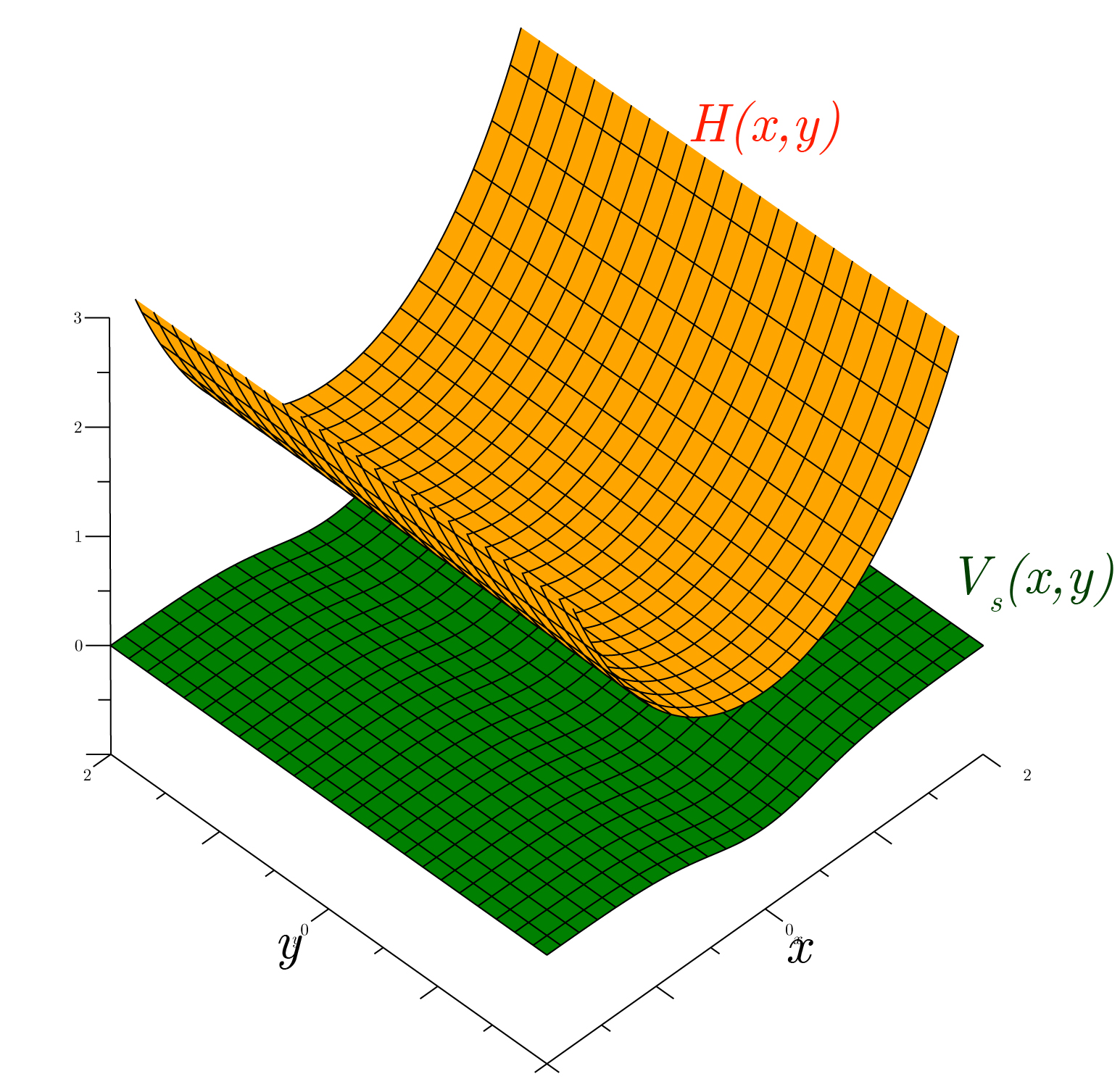
The Catenary surface and the corresponding geometric potential on the surface, observed by the particle.

Considering $\psi_{t}\left(x,y\right)=X\left(x\right)Y\left(y\right)$ one obtains

$$-\frac{\hslash^{2}}{2m}\frac{1}{\cosh\left(\frac{x}{a}\right)}\frac{d}{dx}\left(\frac{1}{\cosh\left(\frac{x}{a}\right)}\frac{d}{dx}\right)X\left(x\right)-\frac{\hslash^{2}}{8m}\frac{1}{a^{2}\cosh^{4}\left(\frac{x}{a}\right)}X\left(x\right)=E_{x}X\left(x\right)$$ (80)

and

$$-\frac{\hslash^{2}}{2m}Y^{\prime\prime}\left(y\right)=E_{y}Y\left(y\right).$$ (81)

Let’s introduce $\alpha=\frac{2mE_{x}}{\hslash^{2}}$ and $\beta=\frac{2mE_{y}}{\hslash^{2}}$ upon which (80) and (81) become

$$-\frac{1}{\cosh\left(\frac{x}{a}\right)}\frac{d}{dx}\left(\frac{1}{\cosh\left(\frac{x}{a}\right)}\frac{d}{dx}\right)X\left(x\right)-\frac{1}{4}\frac{1}{a^{2}\cosh^{4}\left(\frac{x}{a}\right)}X\left(x\right)=\alpha X\left(x\right)$$ (82)

and

$$Y^{\prime\prime}\left(y\right)+\beta Y\left(y\right)=0,$$ (83)

respectively. To solve the $x$-component of the field equations, we introduce a change of variable in the following form

$$q=\sinh\left(\frac{x}{a}\right)$$ (84)

which after some manipulation (82) becomes

$$-X^{\prime\prime}\left(q\right)-\frac{1}{4\left(1+q^{2}\right)^{2}}X\left(q\right)=\mathcal{E}X\left(q\right),$$ (85)

in which $\mathcal{E}=a^{2}\alpha$. The latter equation describes a one-dimensional quantum particle in $q$-space which undergoes a binding potential of the form

$$V\left(q\right)=-\frac{1}{4\left(1+q^{2}\right)^{2}}.$$ (86)

Further, to solve (85) we introduce another change of variable given as $z=-q^{2}$ and $X\left(q\right)=\left(1-z\right)^{\lambda}w\left(z\right)$ with $\lambda=\frac{1}{2}+\frac{\sqrt{5}}{4},$ upon which (85) becomes

$$w^{\prime\prime}+\left(\alpha+\frac{\beta+1}{z}+\frac{\gamma+1}{z-1}\right)w^{\prime}+\left(\frac{\mu}{z}+\frac{\nu}{z-1}\right)w=0$$ (87)

where

$$\alpha=0,\beta=-\frac{1}{2},\gamma=\frac{\sqrt{5}}{2},\mu=-\frac{4E+5+2\sqrt{5}}{16}\text{ and }\nu=\frac{1}{8}\left(\frac{5}{2}+\sqrt{5}\right).$$ (88)

Eq. (87) is the so-called Confluent Heun Differential Equation (CHDE) whose solution is given by

$$w\left(z\right)=C_{1}HeunC\left(\alpha,\beta,\gamma,\delta,\eta,z\right)+C_{2}z^{-\beta}HeunC\left(\alpha,-\beta,\gamma,\delta,\eta,z\right).$$ (89)

Herein, $C_{1}$ and $C_{2}$ are two integration constants and $\delta=\mu+\nu-\frac{\alpha\left(2+\gamma+\beta\right)}{2}=-\frac{\mathcal{E}}{4}$ and $\eta=\frac{\left(\beta+1\right)\left(\alpha-\gamma\right)-\beta}{2}-\mu=\frac{\mathcal{E}}{4}+\frac{9}{16}.$ Hence, the general solution of the Schrödinger equation becomes

$$X\left(q\right)=C_{1}\left(1+q^{2}\right)^{\frac{1}{2}+\frac{\sqrt{5}}{4}}HeunC\left(0,-\frac{1}{2},\frac{\sqrt{5}}{2},-\frac{\mathcal{E}}{4},\frac{\mathcal{E}}{4}+\frac{9}{16},-q^{2}\right)+\\ C_{2}\left(1+q^{2}\right)^{\frac{1}{2}+\frac{\sqrt{5}}{4}}\sqrt{q^{2}}HeunC\left(0,\frac{1}{2},\frac{\sqrt{5}}{2},-\frac{\mathcal{E}}{4},\frac{\mathcal{E}}{4}+\frac{9}{16},-q^{2}\right).$$ (90)

Our detailed numerical analysis reveals that there exists only one bound state with $\mathcal{E}=-0.02892460$, $C_{2}=0,$ and $C_{1}=\frac{1}{\sqrt{6.7406}}.$ Hence, the normalized wave function is found to be

$$X\left(q\right)=\frac{1}{\sqrt{6.7406}}\left(1+q^{2}\right)^{\frac{1}{2}+\frac{\sqrt{5}}{4}}HeunC\left(0,-\frac{1}{2},\frac{\sqrt{5}}{2},-\frac{\mathcal{E}}{4},\frac{\mathcal{E}}{4}+\frac{9}{16},-q^{2}\right)$$ (91)

which together with the potential $V\left(q\right)=-\frac{1}{4\left(1+q^{2}\right)^{2}}$ are plotted in Fig. 3. This figure reveals that the particle is localized around the deep of the surface where the total curvature is maximum.

Figure 3:

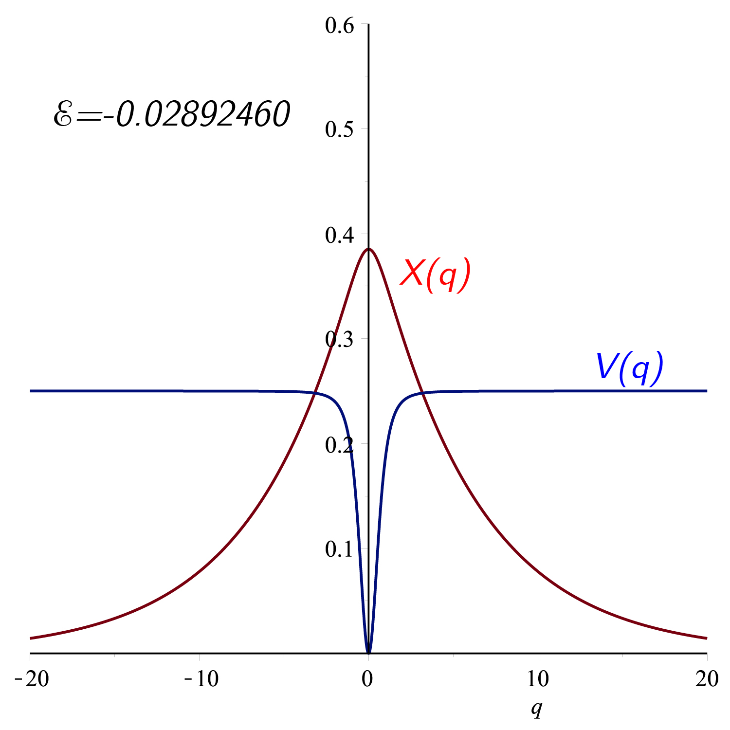
The normalized wave function of the particle confined to move on a Catenary surface together with the pure geometrical potential the particle enconteres in $q$-space.

V Paraboloid of Revolution

Concerning the results of the polar coordinate with radial symmetry, we consider the surface of the paraboloid of revolution which is defined as

$$H\left(\rho\right)=a\left(\frac{\rho}{a}\right)^{2}$$ (92)

where $a$ is a constant parameter with the dimension of length. In Fig. 4 we plot the paraboloid of revolution for $a=1.$ The line element on the surface of the paraboloid of revolution is obtained to be

$$ds^{2}=\left(1+\frac{\rho^{2}}{a^{2}}\right)d\rho^{2}+\rho^{2}d\theta^{2}.$$ (93)

Figure 4:

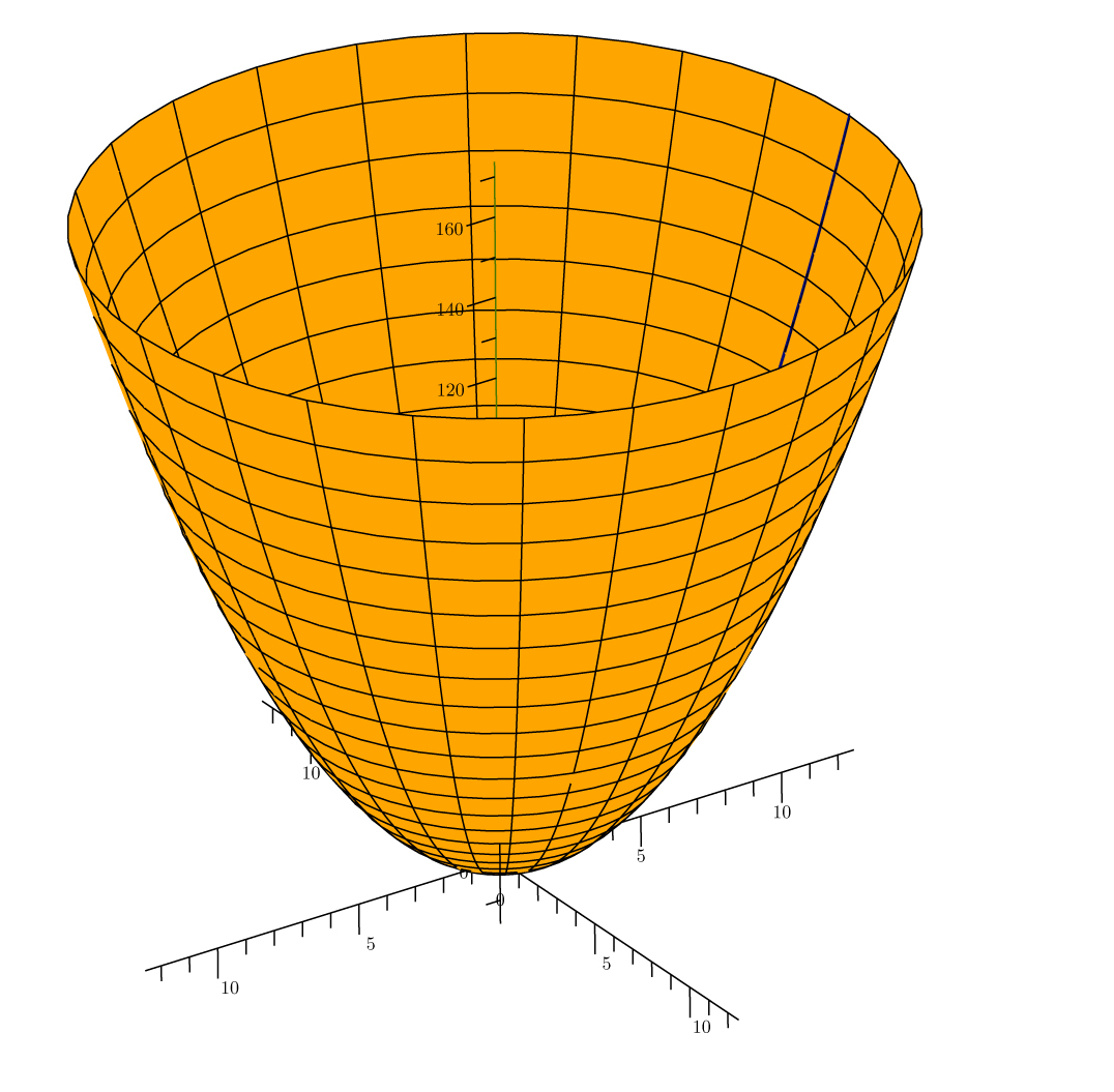
The graph of the Paraboloid of Revolution with $a=1$.

Figure 5:

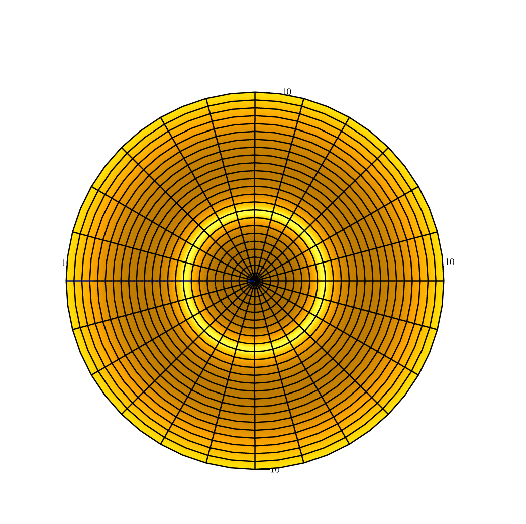
The wave function $\rho\psi_{t}\left(\rho,\theta\right)$ with respect to $\rho$ and $\theta.$ The brightest circle implies the maximum probability of finding the particle on the surface.

Figure 6:

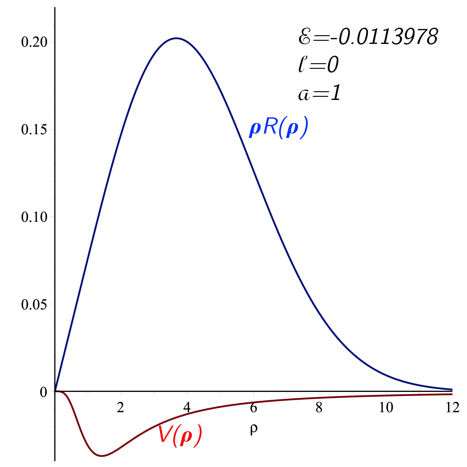
The wave function $\rho R\left(\rho\right)$ versus the potential $V_{S}(\rho)$. The maximum probability doesn’t correspond to the minimum of the potential.

Figure 7:

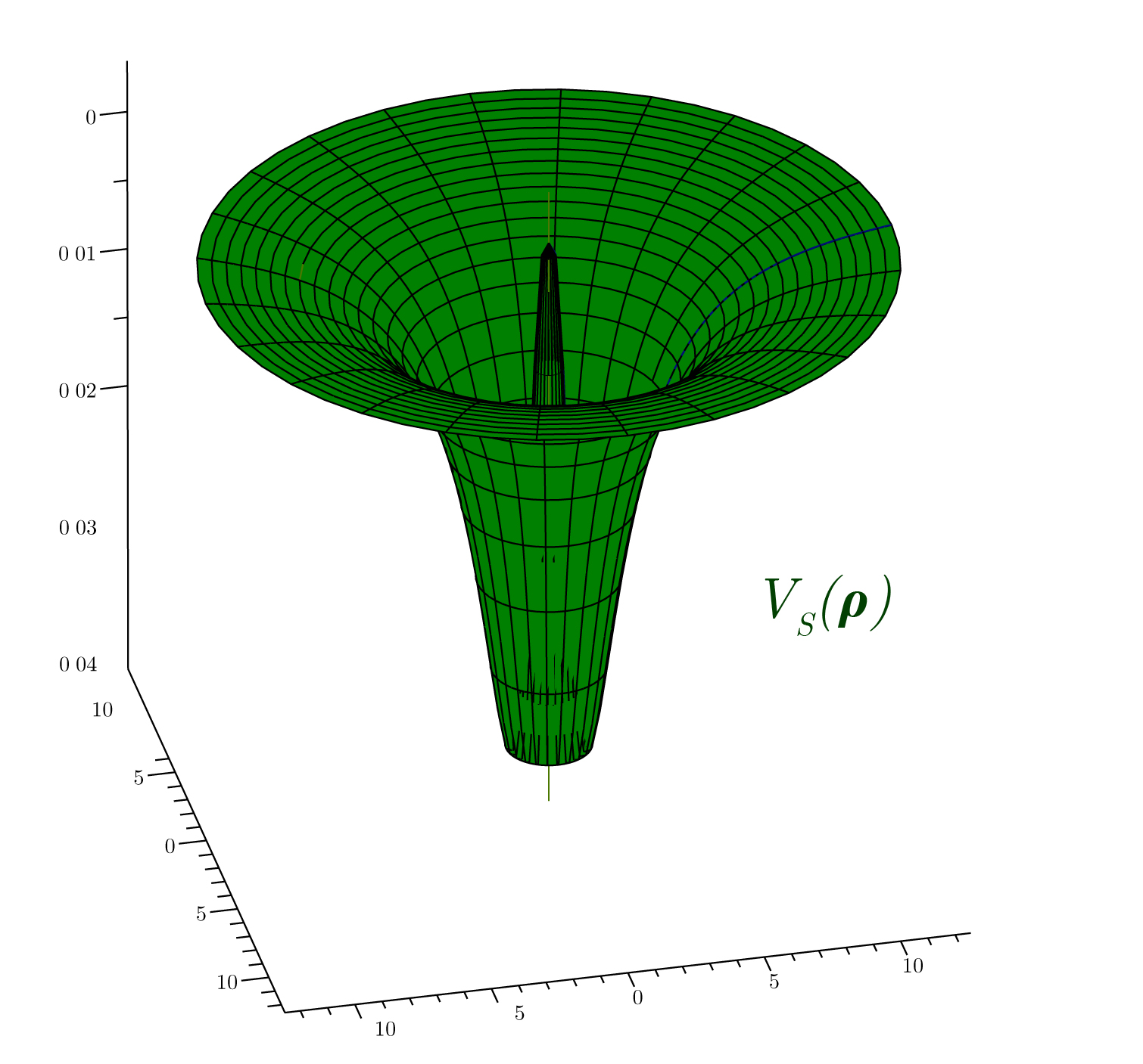
The three dimensional shape of the pure geometric potential experienced by the quantum particle moving on the paraboloid of revolution.

The two dimensional Schrödinger equation on the surface is given by

$$-\frac{\hslash^{2}}{2m}\frac{1}{\sqrt{h}}\partial_{a}\left(\sqrt{h}g^{ab}\partial_{b}\right)\psi_{t}\left(\rho,\theta\right)+V_{S}\left(\rho\right)\psi_{t}\left(\rho,\theta\right)=E_{t}\psi_{t}\left(\rho,\theta\right)$$ (94)

in which

$$V_{S}\left(r\right)=-\frac{\hslash^{2}}{8m}\frac{\rho^{4}}{\left(a^{2}+\rho^{2}\right)^{3}},$$ (95)

$$h=\det g_{ab}=\rho^{2}\left(1+\frac{\rho^{2}}{a^{2}}\right)$$ (96)

and

$$g^{ab}=diag\left[\frac{1}{1+\frac{\rho^{2}}{a^{2}}},\frac{1}{\rho^{2}}\right].$$ (97)

Applying the separating method one obtains

$$\psi_{t}\left(\rho,\theta\right)=R\left(\rho\right)e^{i\ell\theta}$$ (98)

with $\ell=0,\pm 1,\pm 2,...$ and $R\left(r\right)$ satisfying

$$-R^{\prime\prime}-\frac{a^{2}}{\rho\left(a^{2}+\rho^{2}\right)}R^{\prime}+\left(\frac{\ell^{2}\left(a^{2}+\rho^{2}\right)}{a^{2}\rho^{2}}-\frac{\rho^{4}}{4a^{2}\left(a^{2}+\rho^{2}\right)^{2}}\right)R=\frac{a^{2}+\rho^{2}}{a^{2}}\mathcal{E}R$$ (99)

where $\mathcal{E}=\frac{2mE_{t}}{\hslash^{2}}.$ Without going into the details, the general solution of the Schrödinger equation is given in terms of the Confluent Heun function, expressed as

$$R\left(\rho\right)=C_{1}\rho^{\ell}\left(a^{2}+\rho^{2}\right)^{\frac{3+\sqrt{10}}{4}}e^{-\frac{\sqrt{\left|\mathcal{E}\right|}}{2a}\rho^{2}}HeunC\left(a\sqrt{\left|\mathcal{E}\right|},\ell,\frac{\sqrt{10}}{2},-\frac{1}{16}+\frac{\ell^{2}}{4}-\frac{\mathcal{E}a^{2}}{4},\frac{3-\ell^{2}+\mathcal{E}a^{2}}{4},-\frac{\rho^{2}}{a^{2}}\right)+\\ C_{2}\rho^{-\ell}\left(a^{2}+\rho^{2}\right)^{\frac{3+\sqrt{10}}{4}}e^{-\frac{\sqrt{\left|\mathcal{E}\right|}}{2a}\rho^{2}}HeunC\left(a\sqrt{\left|\mathcal{E}\right|},-\ell,\frac{\sqrt{10}}{2},-\frac{1}{16}+\frac{\ell^{2}}{4}-\frac{\mathcal{E}a^{2}}{4},\frac{3-\ell^{2}+\mathcal{E}a^{2}}{4},-\frac{\rho^{2}}{a^{2}}\right),$$ (100)

in which $C_{1}$ and $C-2$ are the integration constants. From the solution (100) we see that with $\ell\geq 0$ the first solution is regular at the origin while for $\ell\leq 0$ the second solution coincides with the first solution (with $\ell\geq 0)$. Knowing also that the sign of $\ell$ doesn’t make any change in the solution, we set $\ell\geq 0$ and eliminate the second solution as it is irregular at the origin. The square integrability of the solution implies

$$\int\nolimits_{0}^{2\pi}\int\nolimits_{0}^{\infty}\left|R\left(\rho\right)e^{i\ell\theta}\right|^{2}\rho^{2}d\rho d\theta=1.$$ (101)

Our numerical calculations revealed that for the ground state where $\ell=0$ the binding energy is given by $\mathcal{E}=-0.0113978$ and $C_{1}=\frac{1}{\sqrt{2\pi}\sqrt{27.268}}.$ In Fig. 5 we plot $\rho\psi_{t}\left(\rho,\theta\right)$ in terms of $\rho$ and $\theta.$ The bright circle is the pick of the wave function indicating the maximum probability radius. In Fig. 6 we plot the normalized wave function $\rho R\left(\rho\right)$ and the potential $V_{S}\left(\rho\right)$ in terms of $\rho$ for $\ell=0$ and $a=1.$ In Fig. 7 we plot a three-dimensional picture of the potential which the particle on the surface observes. We comment finally that for $\ell\geq 0$ there is no bound state solution satisfying the boundary conditions.

VI Conclusion

The nonrelativistic quantum particle confined to a curved surface has been revisited in a more familiar notation and more details. We have studied explicitly the case of the Monge parametrization in two different coordinate systems, i.e., Cartesian and Polar coordinates. We have shown that in the Cartesian coordinate system the geometric effective potential for the small perturbation is simply given by $V_{S}\simeq-\frac{\hslash^{2}}{8m}\left(\left(H_{xx}-H_{yy}\right)^{2}+4H_{xy}^{2}\right)$ which depends on the second derivatives of the height function $H\left(x,y\right).$ The effective Schrödinger equation i.e.,

$$-\frac{\hslash^{2}}{2m}\nabla^{2}\psi_{t}\left(x,y\right)-\frac{\hslash^{2}}{8m}\left(\left(H_{xx}-H_{yy}\right)^{2}+4H_{xy}^{2}\right)\psi_{t}\left(x,y\right)=E_{t}\psi_{t}\left(x,y\right)$$ (102)

with $\nabla^{2}=\frac{\partial^{2}}{\partial x^{2}}+\frac{\partial^{2}}{\partial y^{2}}$ is significantly simpler than the original one. In many cases where the deviation from a flat surface is small, we believe that this equation is a very good and acceptable approximation. In the last part of the paper, we studied two interesting curved surfaces, particularly a Catenoid and a paraboloid of revolution. We solved the corresponding Schrödinger equation of a particle confined on these surfaces without any external potential. We found only one possible bound state for each surface which localizes the particle around the deep of the point of maximum curvature. The exact normalized wave functions with the potentials and the surfaces have been displayed in a number of figures.

References

(1) R. C. T. da Costa, Phys. Rev. A 23, 1982 (1980).
(2) M. Katsnelson, Graphene: Carbon in Two Dimensions
(Cambridge University Press, Cambridge, 2012);
A. H. Castro Neto, F. Guinea, N. M. R. Peres, K. S. Novoselov and A. K.
Geim, The electronic properties of graphene, Rev. Mod. Phys. 81,
109 (2009);
A. K. Geim & K. S. Novoselov, The rise of graphene, Nature Mater 6, 183 (2007).
(3) S. Berber, Y.K. Kwon, D. Tomanek, Unusually High Thermal
Conductivity of Carbon Nanotubes, Phys. Rev. Lett. 84, 4613 (2000).
(4) L. Wei, P. K. Kuo, R. L. Thomas, T. R. Anthony, and W. F.
Banholzer, Thermal conductivity of isotopically modified single crystal
diamond, Phys. Rev. Lett. 70, 3764 (1993);
S. Iijima, Nature (London), Helical microtubules of graphitic carbon,
354, 56 (1991).
(5) A. Carvalho, M. Wang, X. Zhu, A. S. Rodin, H. Su, A. H.
Castro Neto, Phosphorene: from theory to applications, Nat. Rev. Mater.
1, 11 (2016).
(6) M. Deserno, Fluid lipid membranes: From differential geometry
to curvature stresses, Chemistry and Physics of Lipids, 185, 11
(2015).
(7) B. DeWitt, Dynamical Theory in Curved Spaces. I. A Review of
the Classical and Quantum Action Principles, Rev. Mod. Phys. 29,
377 (1957).
(8) R. da Costa, Quantum mechanics of a constrained particle,
Phys. Rev. A 23, 1982 (1981).
(9) G. Ferrari, and G. Cuoghi, Phys. Rev. Lett. 100,
230403 (2008).
(10) F. Serafim, F. A. N. Santos, J. R. F. Lima, S. Fumeron, B.
Berche and F. Moraes, Magnetic and geometric effects on the electronic
transport of metallic nanotubes, J. Appl. Phys. 129, 044301 (2021);
J. D. M. de Lima , E. Gomes1, F. F. da Silva Filho, F. Moraes, and R.
Teixeira, Geometric effects on the electronic structure of curved nanotubes
and curved graphene: the case of the helix, catenary, helicoid, and
catenoid, Eur. Phys. J. Plus 136, 551 (2021).
(11) J. E. G. Silva, J. Furtado, and A. C. A. Ramos, Electronic
properties of a graphene nanotorus under the action of external fields, Eur.
Phys. J. B 93, 225 (2020).
(12) J. E. G. Silva, J. Furtado, T. M. Santiago, A. C.A. Ramos,
D. R. da Costa, Electronic properties of bilayer graphene catenoid bridge,
Phys. Lett. A 384, 126458 (2020).
(13) M. D. Oliveira and A. G. M. Schmidt, Exact solutions of
Schrödinger and Pauli equations for a charged particle on a sphere and
interacting with non-central potentials, J. Math. Phys. 60, 032102
(2019).
(14) A. G. M. Schmidt, Exact solutions of Schrödinger
equation for a charged particle on a sphere and on a cylinder in uniform
electric and magnetic fields, Physica E: Low-dimensional Systems and
Nanostructures, 106, 200 (2019);
(15) A. G. M. Schmidt, Exact Solutions to Schrödinger
Equation for a Charged Particle on a Torus in Uniform Electric and Magnetic
Fields, Brazilian Journal of Physics, 50, 419 (2020).
(16) J. R. F. Lima et al., Effects of rotation on Landau states of
electrons on a spherical shell, Physics Letters A 382, 2499 (2018).
(17) V. Atanasov, and R. Dandoloff, Quantum-elastic bump on
a surface, Eur. J. Phys. 38, 015405 (2017);
P. C. S. Cruzetal, Energy levels of a quantum particle on a cylindrical
surface with non-circular cross-section in electric and magnetic fields,
Annals of Physics 379, 159(2017);
D. Biswas and S. Ghosh, Quantum mechanics of a particle on a torus knot:
Curvature and torsion effects, EPL, 132, 10004 (2020);
M. Encinosa, Coupling curvature to a uniform magnetic field: An analytic and
numerical study, Phys. Rev. A 73, 012102 (2006);
C. Filgueiras, and B. F. de Oliveira, Electron on a cylinder with
topological defects in a homogeneous magnetic field, Ann. Phys. (Berlin)
523, 898 (2011);
V. Atanasov, R. Dandoloff and A. Saxena, Torus in a magnetic field:
curvature-induced surface states, J. Phys. A: Math. Theor. 45,
105307 (2012).
(18) P. C. Schuster and R. L. Jaffe, Quantum mechanics on
manifolds embeddedin Euclidean space, Annals of Physics 307, 132
(2003).