Learning and Adaptation
for Millimeter-Wave Beam Tracking and Training:
a Dual Timescale Variational Framework

Abstract

Millimeter-wave vehicular networks incur enormous beam-training overhead to enable narrow-beam communications. This paper proposes a learning and adaptation framework in which the dynamics of the communication beams are learned and then exploited to design adaptive beam-tracking and training with low overhead: on a long-timescale, a deep recurrent variational autoencoder (DR-VAE) uses noisy beam-training feedback to learn a probabilistic model of beam dynamics and enable predictive beam-tracking; on a short-timescale, an adaptive beam-training procedure is formulated as a partially observable (PO-) Markov decision process (MDP) and optimized via point-based value iteration (PBVI) by leveraging beam-training feedback and a probabilistic prediction of the strongest beam pair provided by the DR-VAE. In turn, beam-training feedback is used to refine the DR-VAE via stochastic gradient ascent in a continuous process of learning and adaptation. The proposed DR-VAE learning framework learns accurate beam dynamics: it reduces the Kullback-Leibler divergence between the ground truth and the learned model of beam dynamics by ${\sim}95\%$ over the Baum-Welch algorithm and a naive learning approach that neglects feedback errors. Numerical results on a line-of-sight scenario with multipath and 3D beamforming reveal that the proposed dual timescale approach yields near-optimal spectral efficiency, and improves it by $130\%$ over a policy that scans exhaustively over the dominant beam pairs, and by $20\%$ over a state-of-the-art POMDP policy. Finally, a low-complexity policy is proposed by reducing the POMDP to an error-robust MDP, and is shown to perform well in regimes with infrequent feedback errors.

I Introduction

Millimeter-wave (mm-wave) has emerged as the most promising technology to enable multi-gigabit rates in vehicular communications, thanks to large bandwidth availability [2]. By operating at carrier frequencies ranging from $30$ up to hundreds of GHz, mm-wave communications suffer from high isotropic path loss, overcome by using large antenna arrays with beamforming [3]. Yet, highly directional communications are susceptible to beam misalignment due to the mobility of the user equipment (UE) or the surrounding propagation environment. Traditional beam-alignment schemes such as exhaustive search [4] suffer from severe overhead, increased communication delay, and degraded spectral efficiency.

To achieve efficient design, adaptive beam-training schemes have been proposed [5, 6, 7, 8, 9], that leverage information on the UE’s mobility and beam-training feedback. In our recent work [7], we showed that statistical knowledge of the UE’s mobility is key to reduce the beam-training overhead and improve spectral efficiency, even in highly mobile V2X scenarios. Yet, the design in [7] relies on accurate statistical knowledge of the beam dynamics, which may need to be estimated from noisy measurements. This observation begs the critical question: How can beam dynamics be estimated and leveraged to optimize beam-training and data communications?

To address this challenge, in this paper we consider a mm-wave vehicular communication scenario, where a UE moves along a road according to an unknown mobility model and is served by a roadside base station (BS). Both UE and BS employ large antenna arrays with 3D beamforming to enable directional communication. The mobility of the UE and the surrounding environment induce dynamics in the strongest beam pair that maximize the beamforming gain; these dynamics could be exploited to enable efficient beam-tracking and training. To learn and exploit these unknown dynamics, we propose a dual timescale learning and adaptation framework: in the long-timescale (of the order of several hundred frames), the BS uses beam-training feedback to learn the strongest beam pair dynamics and enable predictive beam-tracking, using a deep recurrent variational autoencoder (DR-VAE) [10]; in the short-timescale (one frame duration), adaptive beam-training schemes leverage the probabilistic prediction of the strongest beam pair provided by the DR-VAE and beam-training feedback to minimize the overhead and maximize the frame spectral efficiency. In turn, beam-training measurements are used to refine the DR-VAE via stochastic gradient ascent, in a continuous process of learning and adaptation.

We formulate the decision-making process over the short-timescale as a partially observable (PO-) Markov decision process (MDP) and propose a point-based value iteration (PBVI) method that leverages provable structural properties to design an approximately optimal policy, which provides the rule to select beam-training actions based on the belief (probability distribution over the optimal BS-UE beam pair, given the history of actions and beam-training measurements). To trade computational complexity with accuracy, we propose an MDP-based policy that operates under the assumption of error-free beam-training feedback, and an error-robust version that combines MDP-based actions with POMDP-based belief updates: it is shown that the error-robust MDP-based policy can be optimized at a fraction ($\sim$1/5) of the time while achieving spectral efficiency close to the POMDP-based policy in regimes with infrequent feedback errors.

Numerical evaluations using 3D analog beamforming at both BS and UE reveal that the DR-VAE coupled with PBVI-based adaptation reduce the average Kullback-Leibler (KL) divergence between a ground truth Markovian and the learned models by $\sim$95% over the Baum-Welch algorithms [11] and a naive approach that ignores errors in the beam-training measurements, and improve spectral efficiency by $\sim$10%. Finally, we simulate a setting with 2D UE mobility and 3D analog beamforming for two scenarios, one with line-of-sight (LOS) channels, and the other with additional non-LOS (NLOS) multipath: the PBVI policy improves the spectral efficiency over a state-of-the-art short-timescale single shot (STSS) POMDP policy [12] by $16\%$ and $20\%$ in the two scenarios, and outperforms a scheme that scans exhaustively over the dominant beam pairs (EXOS) by $85\%$ and $130\%$, respectively. Similarly, the error-robust MDP policy improves the spectral efficiency by $8\%$ and $7\%$ over the STSS policy and by $70\%$ and $100\%$ over EXOS, respectively.

Related Work: Beam-alignment has been a topic of intense research in the last decade and can be categorized as beam sweeping [13], estimation of angles of arrival (AoA) and departure (AoD) [14], and contextual-information-aided schemes [15, 16, 17, 18, 19, 20]. Despite their simplicity, these schemes do not incorporate mobility dynamics, leading to large beam-training overhead in high mobility scenarios [2]. Moreover, beam-training may still be required to compensate for noise and inaccuracies in contextual information, or due to privacy concerns (e.g., sharing GPS coordinates as in [15, 16, 17, 18]).

Recent works [12, 21, 18, 22, 8, 9, 23, 17] proposed adaptive and machine learning-based solutions exploiting side-information and/or beam-training feedback. For instance, [21] uses the received sounding signal from multiple surrounding BSs to predict the optimal beam via deep learning. In [23], a convolutional neural network is trained based on simulated channels and then used to predict beams via compressive sensing. Reinforcement learning-based beam-alignment schemes have been proposed in [12, 18, 22, 8, 9]. In our previous works [9, 22], we used the beam-training feedback to design adaptive beam-training policies under the assumption of error-free and erroneous beam-training feedback, respectively. In the aforementioned works, mobility is not leveraged in the design, incurring large overhead in high mobility scenarios [2].

To overcome this limitation, in our recent work [7] we showed that, by exploiting the beam dynamics via POMDP, the spectral efficiency of V2X communication is greatly improved over conventional schemes, such as exhaustive search. Similarly, the paper [12] exploits beam dynamics to make beam predictions, and proposes a POMDP-based scheme (evaluated numerically in Sec. V) to maximize the expected spectral efficiency. Yet, these papers assume a priori statistical knowledge of beam dynamics, which need to be learned from noisy beam-training measurements in practice. Without statistical knowledge of beam dynamics, [7] is not amenable to concurrent learning and optimization of the POMDP policy, due to large optimization cost. In contrast to [7], herein, we decouple the beam-training design from the estimation of beam dynamics, by proposing a dual timescale approach in which a stochastic model of beam dynamics is learned on the long-timescale to enable predictive beam-tracking, interleaved with the execution of a beam-training policy in the short-timescale. The beam-training procedure is optimized in the short-timescale (single frame, agnostic to beam dynamics), using beam predictions provided by the long-timescale learning module. We note three advantages of this approach over [7, 12]: 1) since learning the model of beam dynamics is decoupled from the beam-training policy optimization, learning and adaptation can be done concurrently (vs offline model learning required in [7]); 2) the maximization of the frame spectral efficiency (vs average long-term in [7]), favors accurate detection of the optimal BS-UE’s beam pair, which in turn improves the ability to predict optimal beam association for the next frames, and indirectly maximizes spectral efficiency in the long-timescale; 3) by enabling adaptive beam-training of variable duration with multiple beam-training rounds, vs a single-shot beam-training phase of fixed duration of [12], we achieve superior performance, as shown numerically in Sec. V.

Contributions: in a nutshell, we propose a dual timescale approach in which the dynamics of the strongest beam pair are learned over the long-timescale, to enable predictive beam-tracking and efficient beam-training over the short-timescale:

1. We propose a DR-VAE-based learning framework to learn the dynamics of the strongest beam pair, trained via stochastic gradient ascent from beam-training feedback;

2. We formulate a POMDP framework to design beam-training in the short-timescale, with the goal of maximizing the expected frame spectral efficiency, by leveraging predictions provided by the DR-VAE and beam-training feedback. We propose a linear time PBVI algorithm to find an approximately optimal policy, and leverage structural properties to reduce its complexity;

3. For the special case of error-free feedback, we prove that it is optimal to scan the most likely beam pairs, leading to a low-complexity value iteration algorithm. We design an error-robust version that combines MDP-based actions with POMDP-based belief updates, and demonstrate near-optimal performance in regimes with infrequent errors.

The rest of this paper is organized as follows: Sec. II presents the system model; Sec. III describes the POMDP formulation; Sec. IV presents the DR-VAE learning framework; Sec. V provides numerical results, followed by final remarks in Sec. VI.

Notation: $\mathbb{C}$: set of complex numbers; $\mathcal{CN}$: complex Gaussian distribution; $\mathcal{E}(m)$: exponential distribution with mean $m$; $\mathcal{G}$: standard Gumbel distribution; $\mathbb{E}[\cdot]$: expectation operator; $\|\cdot\|_{2}$: L2 norm; $(\cdot)^{\rm H}$: complex conjugate transpose; $\odot$: Hadamard (element-wise) product of two vectors; $\mathbb{I}[\cdot]$: indicator function; $\langle\boldsymbol{\beta},\boldsymbol{\alpha}\rangle=\sum_{i=1}^{n}\boldsymbol{\beta}(i)\boldsymbol{\alpha}(i)$: inner product of $\boldsymbol{\alpha},\boldsymbol{\beta}\in\mathbb{R}^{n}$; $\mathbf{e}_{i}$: standard basis column vector with $\mathbf{e}_{i}(i){=}1$, $\mathbf{e}_{i}(j){=}0,\forall j{\neq}i$; $\mathcal{B}$: probability simplex (of suitable dimension); for a finite discrete set $\mathcal{I}$ and a function $g{:}\mathcal{I}{\mapsto}\mathbb{R}$, $\operatorname*{arg\,max}_{i\in\mathcal{I}}g(i)$ returns an element $i^{*}{\in}\mathcal{I}$ such that $g(i^{*}){=}\max_{i\in\mathcal{I}}g(i)$, with ties broken arbitrarily.

II System Model

We consider a mobile mm-wave vehicular system: a UE is moving along the road, covered by multiple roadside base stations (BSs), and is served by one BS at a time; if it exits the coverage area of its serving BS, handover is performed to the next serving BS. In this paper, we restrict the design to the UE and its serving BS, as depicted in Fig. 1. The BS and UE both use 3D beamforming with large antenna arrays (e.g, uniform planar arrays), with $M_{\rm tx}$ and $M_{\rm rx}$ antennas, respectively (the main system parameters are summarized in Table 1 of Sec. V).

We consider a frame-based system, with frames of duration $T_{\rm fr}$ divided into $K$ slots, each of duration $T_{\rm s}{\triangleq}T_{\rm fr}/K$. To enable beamforming, each frame is split into a beam-training (BT) phase of variable number of slots, followed by data communication (DC) for the remainder of the frame, as shown in Fig. 2. The mobility of the UE and of the surrounding propagation environment induce dynamics in the optimal beam pair that maximize the beamforming gain at the transmitter and receiver (see example of Fig. 1). We assume that the frame duration does not exceed the beam coherence time $T_{b}$ [24], i.e., $T_{\rm fr}\leq T_{b}$, so that the optimal beam pair remain constant during the entire frame duration but may change across frames. For example, using the analysis of [24] for a line of sight (LOS) scenario with beams of $11.25^{\circ}$ beamwidth, operating at a carrier frequency of 30[GHz], we find that $T_{b}{\simeq}400$[ms] for a UE traveling at 108[km/h] at 50[m] from the BS, perpendicular to the beam direction, so that the choice of $T_{\rm fr}{=}20$[ms] (used also in our numerical evaluations) satisfies this assumption.

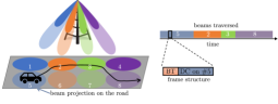
Figure 1: Example of a mm-wave system with one BS and one omni-directional UE (multi-antenna case considered in the paper): as the UE moves across the coverage region, it traverses several communication beams (top right); to enable beamforming, each frame is split into a beam-training (BT) phase followed by data communication (DC) for the rest of the frame (bottom right).

The goal of this paper is to learn these beam-dynamics to enable predictive beam-tracking and design adaptive BT techniques with improved spectral efficiency. To this end, we propose a dual timescale learning and adaptation framework, depicted as a block diagram in Fig. 2: in the long-timescale (the time interval during which the UE stays within the BS’ coverage area, of the order of several hundred frames) a model of beam dynamics is learned, to enable predictive beam-tracking; in the short-timescale (one frame duration), an adaptive BT policy is designed to maximize the expected frame spectral efficiency, by exploiting a probabilistic beam prediction (prior belief) provided by the beam dynamics learning module and BT feedback. Specifically:

1. Modeling the dynamics of the strongest beam pair index (SBPI, the index of the beamforming vectors that maximize the expected beamforming gain, averaged over small-scale conditions) as a Markov process, the BS leverages a learned SBPI’s transition model to provide probabilistic predictions over SBPIs (prior belief) at the start of each frame;

2. The prior belief and BT feedback are leveraged to optimize the beam-training process on the short-timescale to maximize the spectral efficiency via POMDP (Sec. III);

3. The Markov SBPI model is continuously learned via a DR-VAE-based framework (Sec. IV), based on BT feedback collected in the observation buffer.

Next, we describe the model features and abstractions used.

II-A Signal and Channel Models

Let $\mathbf{x}_{t,k}{\in}\mathbb{C}^{L_{\rm sy}\times 1}$ be the sequence of $L_{\rm sy}$ symbols transmitted by the BS in slot $k{\in}\mathcal{K}{\triangleq}\{0,1,\cdots,K{-}1\}$ of frame $t\in\mathbb{N}$, with $\mathbb{E}[\|\mathbf{x}_{t,k}\|_{2}^{2}]{=}L_{\rm sy}$. The corresponding signal received at the UE, $\mathbf{y}_{t,k}\in\mathbb{C}^{L_{\rm sy}\times 1}$, is expressed as

$$\mathbf{y}_{t,k}=\sqrt{P_{t,k}}\cdot(\mathbf{f}_{t,k}^{\rm H}\mathbf{H}_{t,k}\mathbf{c}_{t,k})\cdot{\mathbf{x}_{t,k}}+\mathbf{w}_{t,k},$$ (1)

where: $P_{t,k}$ is the average transmit power of the BS; $\mathbf{H}_{t,k}{\in}\mathbb{C}^{M_{\rm rx}\times M_{\rm tx}}$ is the channel matrix; $\mathbf{w}_{t,k}{\in}\mathbb{C}^{L_{\rm sy}\times 1}$ is the AWGN with variance $\sigma_{w}^{2}$, $\mathbf{w}_{t,k}{\sim}\mathcal{CN}(\boldsymbol{0},\sigma_{w}^{2}\mathbf{I})$; $\mathbf{c}_{t,k}{\in}\mathcal{C}$ and $\mathbf{f}_{t,k}{\in}\mathcal{F}$ are unit-norm beamforming vectors at the BS and UE, taking values from pre-designed analog beamforming codebooks $\mathcal{C}{\subset}\mathbb{C}^{M_{\rm tx}\times 1}$ and $\mathcal{F}{\subset}\mathbb{C}^{M_{\rm rx}\times 1}$, respectively. We index all possible beamforming vector pairs of the BS and UE with the beam pair index (BPI) $j{\in}\mathcal{S}{\triangleq}\{1,\cdots,|\mathcal{C}||\mathcal{F}|\}$, so that $(\mathbf{c}^{(j)},\mathbf{f}^{(j)}){\in}\mathcal{C}{\times}\mathcal{F}$ is the $j$th beam pair.

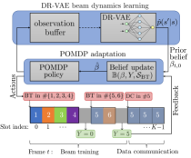
Figure 2: Dual timescale framework (short- and long-timescale interactions shown with solid and dashed arrows, respectively) and example of POMDP policy, based on Fig. 1, with the UE in the strongest beam pair index (BPI) $5$: the BS executes BT on the set of BPIs $\{1,2,3,4\}$ over 4 consecutive slots, receives the feedback signal $Y{=}0$ (indicating the misalignment condition), then executes BT on the set of BPIs $\{5,6\}$ over two consecutive slots, receives the feedback signal $Y{=}5$ (indicating alignment on BPI 5); finally, it terminates BT and executes DC on the detected BPI $5$, until the end of the frame.

In this paper, we adopt a multipath channel model with a LOS path [9, 25, 26], expressed as

$$\mathbf{H}_{t,k}{=}\sum_{\ell=0}^{N_{P}}\sqrt{M_{\rm tx}M_{\rm rx}}\cdot h_{t,k}^{(\ell)}\cdot\Big{(}\mathbf{d}_{\rm rx}(\theta_{t}^{(\ell)})\cdot\mathbf{d}_{\rm tx}(\phi_{t}^{(\ell)})^{\rm H}\Big{)},$$ (2)

where $h_{t,k}^{(0)}{\sim}\mathcal{CN}(0,1/{\rm PL}_{t})$ is the complex gain of the LOS path, with pathloss ${\rm PL}_{t}{=}(4\pi d_{t})^{2}/\lambda_{c}^{2}$, function of the UE-BS’ distance $d_{t}$ and the carrier wavelength $\lambda_{c}$; $\theta_{t}^{(0)}$ and $\phi_{t}^{(0)}$ are the AoA and AoD of the LOS path (including both azimuth and elevation coordinates, since we use a 3D beamforming architecture), respectively; $\mathbf{d}_{\rm tx}(\cdot)$ and $\mathbf{d}_{\rm rx}(\cdot)$ are the unit norm array response vectors of the BS’ and UE’s antenna arrays, respectively. The components indexed by $\ell{\geq}1$ denote $N_{P}$ additional non-LOS (NLOS) paths, each with their own fading coefficient $h_{t,k}^{(\ell)}{\sim}\mathcal{CN}(0,\sigma_{\ell,t}^{2})$, AoA $\theta_{t}^{(\ell)}$ and AoD $\phi_{t}^{(\ell)}$.

As observed in [27], $d_{t}$, $\theta_{t}^{(\ell)}$, $\phi_{t}^{(\ell)}$ and $\sigma_{\ell,t}^{2}$ are large-scale channel propagation features, hence remain (approximately) constant during the frame duration, as reflected by the assumption $T_{\rm fr}{\leq}T_{b}$ discussed earlier. On the other hand, the small-scale fading coefficients $h_{t,k}^{(\ell)}$ are fast-fading components, and are thus modeled as i.i.d over the slots within the frame. In principle, the beamforming vectors $\mathbf{f}_{t,k}$ and $\mathbf{c}_{t,k}$ should be chosen to maximize the beamforming gain based on the instantaneous channel realization $\mathbf{H}_{t,k}$, by solving $\max_{j\in\mathcal{S}}|\mathbf{f}^{(j)\rm H}\mathbf{H}_{t,k}\mathbf{c}^{(j)}|^{2}$. However, as also noted in [27], doing so requires CSI at both transmitter and receiver, which may be unfeasible in large antenna systems. An alternative approach used in this paper is known as long-term beamforming [27, 28], in which the beamforming vectors are optimized to the large-scale features but not the small-scale ones: the goal is to maximize the expected beamforming gain $G_{t}$, averaged over the small-scale fading coefficients with the large-scale features kept constant, expressed as a function of the beamforming vectors $(\mathbf{c},\mathbf{f})$ as

$$G_{t}(\mathbf{c},\mathbf{f})\triangleq G_{t}^{\rm LOS}(\mathbf{c},\mathbf{f})+G_{t}^{\rm NLOS}(\mathbf{c},\mathbf{f}),$$ (3)

where

$$G_{t}^{\rm LOS}(\mathbf{c},\mathbf{f}) \triangleq\frac{M_{\rm tx}M_{\rm rx}}{{\rm PL}_{t}}|\mathbf{d}_{\rm tx}(\phi_{t}^{(0)})^{\rm H}\mathbf{c}|^{2}|\mathbf{d}_{\rm rx}(\theta_{t}^{(0)})^{\rm H}\mathbf{f}|^{2},\!\!$$ (4)

$$G_{t}^{\rm NLOS}(\mathbf{c},\mathbf{f}) \triangleq\!M_{\rm tx}M_{\rm rx}\!\!\sum_{\ell=1}^{N_{P}}\sigma_{\ell,t}^{2}|\mathbf{d}_{\rm tx}(\phi_{t}^{(\ell)})^{\rm H}\mathbf{c}|^{2}|\mathbf{d}_{\rm rx}(\theta_{t}^{(\ell)})^{\rm H}\mathbf{f}|^{2}$$

are the expected gains along the LOS and NLOS paths. The maximum expected beamforming gain is then $G_{t}^{\max}{=}\max_{j\in\mathcal{S}}G_{t}(\mathbf{c}^{(j)}{,}\mathbf{f}^{(j)})$, maximized by the optimal BPI.

Channel measurements [27] have shown that, even in dense urban environments, the mm-wave channel typically exhibits 1-3 paths, with the LOS one containing most of the signal energy, implying that $\sum_{\ell=1}^{N_{P}}\sigma_{\ell,t}^{2}{\ll}1/{\rm PL}_{t}$. Based on this fact, in this paper we assume that the maximum expected beamforming gain is achieved along the LOS path,

$$G_{t}^{\max}\approx\max_{j\in\mathcal{S}}G_{t}^{\rm LOS}(\mathbf{c}^{(j)},\mathbf{f}^{(j)}),$$ (5)

and is thus maximized by the strongest BPI (SBPI)

$$S_{t}=\operatorname*{arg\,max}_{j\in\mathcal{S}}G_{t}^{\rm LOS}(\mathbf{c}^{(j)},\mathbf{f}^{(j)}),$$ (6)

so that $(\mathbf{c}^{(S_{t})},\mathbf{f}^{(S_{t})})$ should be used at the BS and UE to maximize the expected beamforming gain in frame $t$.

II-B Sectored antenna with binary SNR model

We now approximate the beamforming gain using a sectored antenna model [5, 9, 7], which provides an analytically tractable yet valuable approximation of the actual beam pattern, as demonstrated numerically in Sec. V. To develop this model, note that there is a relationship between the UE’s position and the pathloss, AoA and AoD of the LOS path, denoted as ${\rm PL}(x)$, $\theta(x)$ and $\phi(x)$ for a UE in position $x\in\mathcal{X}$ within the coverage area $\mathcal{X}$ of the BS. From (4), the expected beamforming gain along the LOS path is then expressed as

$$G^{\rm LOS}(\mathbf{c},\mathbf{f},x)\triangleq\frac{M_{\rm tx}M_{\rm rx}}{{\rm PL}(x)}|\mathbf{d}_{\rm tx}(\phi(x))^{\rm H}\mathbf{c}|^{2}|\mathbf{d}_{\rm rx}(\theta(x))^{\rm H}\mathbf{f}|^{2},$$

for a UE in position $x$, and the SBPI as

$$s^{*}(x)\triangleq\arg\max_{j\in{\mathcal{S}}}\ G^{\rm LOS}(\mathbf{c}^{(j)},\mathbf{f}^{(j)},x).$$ (7)

With this definition, we partition the coverage area $\mathcal{X}$ into irregularly shaped sectors $\{\mathcal{X}_{j}\}_{j{\in}\mathcal{S}}$, with $\mathcal{X}_{j}{\triangleq}\{x{\in}\mathcal{X}{:}s^{*}(x){=}j\}$ representing the set of positions in which the $j$th BPI maximizes the expected beamforming gain (i.e., it is the SBPI).

Let $X_{t}$ be the position of the UE in frame $t$, so that $S_{t}{=}s^{*}(X_{t})$ is the corresponding SBPI, and consider the $j$th BPI. We denote the condition $X_{t}{\in}\mathcal{X}_{j}$ (or equivalently, $S_{t}{=}j$) as the beam-alignment condition along BPI $j$: in fact, when $S_{t}{=}j$, the $j$th BS’ and UE’s beamforming vector pair maximize the expected beamforming gain along the LOS path, as expressed by (5) and (6); we let ${\rm SNR}_{\rm BA}$ be the expected SNR under the beam-alignment condition, averaged over the small-scale fading coefficients. This SNR requirement may be achieved via power control at the BS, to provide uniform signal quality over the coverage area. In fact, from the signal model (1) and using (3), the expected SNR (averaged over small-scale fading) in position $X_{t}{\in}\mathcal{X}_{j}$ under the $j$th BPI is expressed as

$$\!\!\!\mathbb{E}[{\rm SNR}_{t,k}]{=}\frac{P_{t,k}}{\sigma_{w}^{2}}G_{t}(\mathbf{c}^{(j)},\mathbf{f}^{(j)}){\geq}\frac{P_{t,k}}{\sigma_{w}^{2}}G^{\rm LOS}(\mathbf{c}^{(j)},\mathbf{f}^{(j)},X_{t}),\!\!\!$$ (8)

so that the condition $\mathbb{E}[{\rm SNR}_{t,k}]\geq{\rm SNR}_{\rm BA}$ over $\mathcal{X}_{j}$ under the $j$th BPI is guaranteed by choosing the BS’ transmit power as

$$P_{t,k}=\frac{\sigma_{w}^{2}\cdot{\rm SNR}_{\rm BA}}{\min_{x\in\mathcal{X}_{j}}G^{\rm LOS}(\mathbf{c}^{(j)},\mathbf{f}^{(j)},x)}\triangleq P^{(j)}.$$ (9)

Conversely, we denote $X_{t}{\notin}\mathcal{X}_{j}$ (i.e, $S_{t}{\neq}j$) as the beam-misalignment condition along BPI $j$. In this case, the expected beamforming gain is not maximized, yielding smaller expected SNR. Since the beam-misalignment condition implies $G_{t}(\mathbf{c}^{(j)},\mathbf{f}^{(j)}){<}G_{t}^{\max}$, we upper bound the expected SNR as $\frac{P^{(j)}}{\sigma_{w}^{2}}G_{t}(\mathbf{c}^{(j)},\mathbf{f}^{(j)}){\leq}\rho{\cdot}{\rm SNR}_{\rm BA}$, where $\rho{<}1$ is the misalignment to alignment gain ratio, which accounts for the effect of sidelobes and NLOS multipath.

We have thus defined a binary SNR model, in which the expected SNR is only a function of the beam-alignment condition under the current choice of the BPI $j$: under beam-alignment ($j{=}S_{t}$), the expected SNR is (at least) ${\rm SNR}_{\rm BA}$; under beam-misalignment ($j{\neq}S_{t}$), the expected SNR is (at most) $\rho{\cdot}{\rm SNR}_{\rm BA}$; in this latter case, data communication is in outage since $\rho{\ll}1$. Note that it is desirable for ${\rm SNR}_{\rm BA}$ to be as large as possible, to maximize spectral efficiency; conversely, $\rho$ should be as small as possible to minimize errors in the detection of the SBPI (which explains the use of an upper bound on the expected SNR under beam-misalignment, as a worst case condition); additionally, the power ratio $\max_{j\in\mathcal{S}}P^{(j)}/\min_{j\in\mathcal{S}}P^{(j)}$ should be as small as possible to minimize the peak-to-average power ratio at the BS. These goals may be achieved via careful planning at deployment phase, including BS placement and beam design. We refer to Table 1 in Sec. V for an example of numerical values.

II-C Beam Training (BT) and Data Communication (DC)

We now introduce the BT and DC operations. The goal of the BT phase (of variable duration) is to detect the SBPI $S_{t}$, so that data communication can be performed with maximum expected beamforming gain (averaged over the small-scale fading) for the remainder of the frame. Both operations are executed within the frame duration, and the process is repeated in each frame, based on a POMDP policy described in Sec. III.

BT phase: During the BT phase, the BS selects and executes a sequence of BT actions. A single BT action specifies a set of BPIs ${\mathcal{S}}_{\rm BT}{\subseteq}\mathcal{S}$ to be scanned, selected by the POMDP controller (Sec. III); it is then executed as follows:

1. A sequence of beacon signals $\mathbf{x}$ is sent over the set of BPIs ${\mathcal{S}}_{\rm BT}$, using one slot for each BPI in ${\mathcal{S}}_{\rm BT}$ (the scanning order is unimportant). Let $k_{j}$ be the slot during which BPI $j{\in}{\mathcal{S}}_{\rm BT}$ is scanned: in this slot, the BS transmits with beamforming vector $\mathbf{c}^{(j)}$ and transmit power $P^{(j)}$, while the UE receives synchronously with combining vector $\mathbf{f}^{(j)}$; the UE then processes the received signal $\mathbf{y}_{t,k_{j}}$ (see (1)) using a matched filter, to estimate the SNR along BPI $j$ as

   $$\Gamma_{t}^{(j)}\triangleq\frac{|\mathbf{x}^{\rm H}\mathbf{y}_{t,k_{j}}|^{2}}{\sigma_{w}^{2}\|\mathbf{x}\|_{2}^{2}}.$$ (10)

2. After collecting the sequence $\{\Gamma_{t}^{(j)},\forall j{\in}{\mathcal{S}}_{\rm BT}\}$, the UE transmits a discrete feedback signal $Y$ back to the BS in the next slot. To generate $Y$, the UE first detects the strongest BPI $J{\triangleq}\operatorname*{arg\,max}_{{j}\in{\mathcal{S}}_{\rm BT}}\Gamma_{t}^{(j)}$. If $\Gamma_{t}^{(J)}{>}\eta$ (an SNR threshold $\eta$, designed to trade off false-alarm and misdetection probabilities, as discussed next), then $Y{=}J$ indicates the index of the SBPI detected; otherwise ($\Gamma_{t}^{(J)}{\leq}\eta$), $Y{=}0$ indicates detection of the beam-misalignment condition over ${\mathcal{S}}_{\rm BT}$.

Since the BT action over the BPI set ${\mathcal{S}}_{\rm BT}$ contains $|{\mathcal{S}}_{\rm BT}|$ BPIs, it takes $|{\mathcal{S}}_{\rm BT}|+1$ slots (including the sequential beacons and feedback signal transmissions). Note that the BT action and the feedback signal may be coordinated using low frequency control channels, with small overhead: ${\mathcal{S}}_{\rm BT}{\subseteq}\mathcal{S}$ can be encoded using $|\mathcal{S}|$ bits, and the feedback signal $Y{\in}\mathcal{S}{\cup}\{0\}$ can be encoded using at most $\log_{2}(|\mathcal{S}|+1)$ bits.

We now discuss the feedback distribution $\mathbb{P}_{Y}(y|s,{\mathcal{S}}_{\rm BT})\triangleq\mathbb{P}(Y=y|S_{t}=s,{\mathcal{S}}_{\rm BT})$, denoting the probability of generating the feedback signal $Y=y$, given the ground truth SBPI $S_{t}$ and the BT action over the BPI set ${\mathcal{S}}_{\rm BT}$. Its expression is provided in closed-form in [7]. Consider the case $s\in{\mathcal{S}}_{\rm BT}$ first, i.e., the ground truth SBPI is scanned during the BT action: we define

$$p_{\rm corr}\triangleq\mathbb{P}_{Y}(s|s,{\mathcal{S}}_{\rm BT}),\ p_{\rm md}\triangleq\mathbb{P}_{Y}(0|s,{\mathcal{S}}_{\rm BT})$$

as the probabilities of correctly detecting the SBPI ($Y{=}s$), and of incorrectly detecting beam-misalignment ($Y{=}0$). Then, the SBPI is incorrectly detected ($Y{\neq}s$ and $Y{\neq}0$) with probability

$$\mathbb{P}_{Y}(y|s,{\mathcal{S}}_{\rm BT})=\frac{1-p_{\rm corr}-p_{\rm md}}{|{\mathcal{S}}_{\rm BT}|-1},\ \forall y\in{\mathcal{S}}_{\rm BT}\setminus\{s\},$$

i.e., detection errors are uniform over the remaining BPIs ${\mathcal{S}}_{\rm BT}{\setminus}\{s\}$ (this property follows from the binary SNR model). On the other hand, if $s{\notin}{\mathcal{S}}_{\rm BT}$, i.e., the ground truth SBPI is not scanned during the BT action, we let $p_{\rm fa}$ be the false-alarm probability that beam-alignment is detected, so that

$$\begin{cases}\mathbb{P}_{Y}(y|s,{\mathcal{S}}_{\rm BT})=\frac{p_{\rm fa}}{|{\mathcal{S}}_{\rm BT}|},\ \forall y\in{\mathcal{S}}_{\rm BT},\\ \mathbb{P}_{Y}(0|s,{\mathcal{S}}_{\rm BT})=1-p_{\rm fa},\end{cases}$$

i.e., false-alarm errors are uniform across the set of BPIs ${\mathcal{S}}_{\rm BT}$ scanned during BT (as a result of the binary SNR model).

The threshold $\eta$ trades off false-alarm and misdetection probabilities: if $S_{t}{\notin}{\mathcal{S}}_{\rm BT}$, then beam-misalignment is correctly detected ($Y{=}0$) if and only if $\Gamma_{t}^{(j)}{<}\eta,\forall j{\in}{\mathcal{S}}_{\rm BT}$, yielding

$$p_{\rm fa}=1-\mathbb{P}(\Gamma_{t}^{(j)}<\eta,\forall j\in{\mathcal{S}}_{\rm BT}|S_{t}\notin{\mathcal{S}}_{\rm BT})$$

$$=1-\Big{(}1-e^{-\frac{\eta}{1+\rho\cdot{\rm SNR}_{\rm BA}L_{\rm sy}}}\Big{)}^{|{\mathcal{S}}_{\rm BT}|},$$ (11)

where, using the binary SNR model of Sec. II-B, we used the fact that $\Gamma_{t}^{(j)}{\sim}{\mathcal{E}}(1{+}\rho{\cdot}{\rm SNR}_{\rm BA}L_{\rm sy}),\forall j{\neq}S_{t}$, independently across $j$. On the other hand, if $S_{t}\in{\mathcal{S}}_{\rm BT}$ (the SBPI $S_{t}$ is scanned), then the misalignment condition $Y{=}0$ is incorrectly detected if and only if $\Gamma_{t}^{(j)}{<}\eta,\forall j\in{\mathcal{S}}_{\rm BT}$, yielding

$$p_{\rm md}=\mathbb{P}(\Gamma_{t}^{(j)}<\eta,\forall j\in{\mathcal{S}}_{\rm BT}|S_{t}\in{\mathcal{S}}_{\rm BT})$$ (12)

$$=\Big{(}1-e^{-\frac{\eta}{1+{\rm SNR}_{\rm BA}L_{\rm sy}}}\Big{)}\cdot\Big{(}1-e^{-\frac{\eta}{1+\rho\cdot{\rm SNR}_{\rm BA}L_{\rm sy}}}\Big{)}^{|{\mathcal{S}}_{\rm BT}|-1},$$

where we used $\Gamma_{t}^{(s)}{\sim}{\mathcal{E}}(1{+}{\rm SNR}_{\rm BA}L_{\rm sy})$ along the SBPI $s{=}S_{t}$. In this paper, we set $\eta$ so that $p_{\rm fa}{=}p_{\rm md}$, determined via the bisection method, by leveraging the facts that $p_{\rm fa}$ and $p_{\rm md}$ are increasing and decreasing functions of $\eta$, respectively. However, the following results hold for a generic choice of $\eta$.
DC phase: At the start of the DC phase, in slot $k_{\rm DC}$ within the frame, the BS selects a BPI $s_{\rm DC}$ (both $k_{\rm DC}$ and $s_{\rm DC}$ are selected by the POMDP controller of Sec. III). Data communication then occurs for the remaining $K-k_{\rm DC}$ slots until the end of the frame, with a fixed rate $R$ using the selected BPI: the BS transmits with beamforming vector $\mathbf{c}^{(s_{\rm DC})}$ and transmit power $P^{(s_{\rm DC})}$ given by (9), while the UE receives with combining vector $\mathbf{f}^{(s_{\rm DC})}$. If $S_{t}\neq s_{\rm DC}$, then the beam-misalignment condition occurs, and communication is in outage; otherwise (beam-alignment condition $S_{t}{=}s_{\rm DC}$), outage occurs if $R{>}W_{\rm tot}\log_{2}(1+{\rm SNR}_{t,k})$, where ${\rm SNR}_{t,k}$ is the instantaneous SNR, function of the small-scale fading conditions, $W_{\rm tot}$ is the bandwidth. Owing to the binary SNR model of Sec. II-B, it follows that ${\rm SNR}_{t,k}\sim\mathcal{E}({\rm SNR}_{\rm BA})$ under the beam-alignment condition, yielding the success probability with respect to the small-scale fading conditions

$$\mathbb{P}_{\rm succ}{=}\mathbb{P}\Bigr{(}{\rm SNR}_{t,k}{>}2^{R/W_{\rm tot}}{-}1\Bigr{)}{=}e^{{-}\frac{2^{R/W_{\rm tot}}{-}1}{{\rm SNR}_{\rm BA}}}.$$ (13)

We define the expected frame spectral efficiency, averaged over the small-scale fading, as a function of $k_{\rm DC}$, $s_{\rm DC}$ and the unknown ground truth SBPI $S_{t}{=}s$, as

$${\rm SE}_{\rm fr}(k_{\rm DC},s_{\rm DC};s)={\rm SE}_{\rm BA}{\cdot}\Big{(}1{-}\frac{k_{\rm DC}}{K}\Big{)}\cdot\mathbb{I}[s=s_{\rm DC}],$$ (14)

where ${\rm SE}_{\rm BA}{\triangleq}\frac{\mathbb{P}_{\rm succ}R}{W_{\rm tot}}$ is the expected spectral efficiency under the maximum beamforming condition, $1{-}\frac{k_{\rm DC}}{K}$ is the loss due to the BT overhead, and $\mathbb{I}[s{=}s_{\rm DC}]$ captures the outage condition under beam-misalignment.

II-D SBPI dynamics

The mobility of the UE induces temporally correlated dynamics on the SBPI $S_{t}$, which we exploit to reduce the BT overhead via predictive beam-tracking. In principle, the sequence $\{S_{t},t{\geq}0\}$ may not satisfy the Markov property (for instance, a vehicle moving at constant speed along a road would spend a deterministic amount of time on each SBPI traversed along the path). In this paper, for analytical and computational tractability, we model $\{S_{t},t{\geq}0\}$ as Markovian. We will demonstrate numerically in Sec. V that this assumption yields a good approximation of non-Markovian dynamics. In addition, we assume that the associated Markov chain is time-homogeneous, so that the transition model does not change with time: in fact, long-term mobility patterns typically vary slowly compared to the timescales of the communication scenario under consideration. Let $p(s^{\prime}|s)\triangleq\mathbb{P}(S_{t+1}{=}s^{\prime}|S_{t}{=}s),\forall s{\in}\mathcal{S},\forall s^{\prime}{\in}\mathcal{S}\cup\{\bar{s}\}$ be the one-frame transition probability from the current SBPI $s$ to the next SBPI $s^{\prime}$; the additional state $\bar{s}$ indicates that the UE exited the BS coverage area and can no longer be served by it.

In practice, $p(\cdot|\cdot)$ is unknown and needs to be estimated via BT feedback – a departure from [12] and our previous work [7], which assumed prior knowledge of $p(\cdot|\cdot)$. A naive approach estimates $p(\cdot|\cdot)$ based on the sequence $\{(\hat{s}_{t},\hat{s}_{t+1}),t{\in}\mathcal{T}\}$ of SBPIs’ transitions detected via BT (e.g., exhaustive search) at time frames $t{\in}\mathcal{T}$, as

$$\hat{p}(s^{\prime}|s)=\frac{\sum_{t\in\mathcal{T}}\mathbb{I}[\hat{s}_{t}=s,\hat{s}_{t+1}=s^{\prime}]}{\sum_{t\in\mathcal{T}}\mathbb{I}[\hat{s}_{t}=s]},\ \forall s,s^{\prime}\in\mathcal{S}.$$ (15)

Yet, detection errors caused by noise, beam imperfections, and NLOS multipath may degrade the estimation quality, hence the performance of adaptive BT schemes based on it. The design of an estimation procedure robust to these errors is developed in Sec. IV using a novel technique based on a deep recurrent variational autoencoder (DR-VAE) architecture.

III Short Timescale: adaptive BT via PBVI

This section introduces the POMDP adaptation and proposes an efficient PBVI algorithm to determine an approximately optimal BT policy. Since the short-timescale adaptation is the same for all frames, we do not express the dependence on the frame index $t$, whenever unambiguous. The goal is to design a policy $\pi$ that dictates the sequence of BT/DC actions, so as to to maximize the expected frame spectral efficiency:

$$\!\!\textbf{[MAX-SE]:}\ \max_{\pi}\mathbb{E}_{\pi}\Big{[}{\rm SE}_{\rm fr}(k_{\rm DC},s_{\rm DC};S)\Big{|}S{\sim}\boldsymbol{\beta}_{0}\Big{]},\!$$ (16)

where $\boldsymbol{\beta}_{0}(s){=}\mathbb{P}(S{=}s)$ is the probability mass function of the SBPI $S$ at the start of the frame, provided by the DR-VAE (Sec. IV); the expectation is with respect to $S{\sim}\boldsymbol{\beta}_{0}$, the sequence of actions and observations dictated by policy $\pi$. Since the state $S$ is unknown, we formulate this optimization as a POMDP, with individual components defined as follows.

Time horizon: the slots within the frame $\mathcal{K}{=}\{0,{\cdots},K{-}1\}$.

State: the SBPI $S{\in}\mathcal{S}$, taking value from the state space $\mathcal{S}$; $S$ remains constant during the frame duration, but may change from one frame to the next according to $p(\cdot|\cdot)$ (see Sec. II-D).

Action and reward models: In slot $k$ within the frame, the BS selects whether to perform BT or DC, and on which BPIs. If the DC action is selected on the BPI $s_{\rm DC}{\in}\mathcal{S}$, then data communication occurs over the BPI $s_{\rm DC}$ for the remainder of the frame, as described in Sec. II-C, and the decision period within the current frame terminates. With the goal stated in [MAX-SE], the reward under the DC action is ${\rm SE}_{\rm fr}(k,s_{\rm DC};S)$ as in (14). On the other hand, if the BT action is selected over the set of BPIs ${\mathcal{S}}_{\rm BT}$, then the BS proceeds with a round of BT, which occupies $|{\mathcal{S}}_{\rm BT}|{+}1$ slots for the sequential beacon and feedback signal transmissions (see Sec. II-C). The next BT or DC decision is then taken in slot $k{+}|{\mathcal{S}}_{\rm BT}|{+}1$ of the current frame. Since a BT action must terminate before the end of the frame, the BT action space in slot $k$ is $\mathcal{A}_{{\rm BT},k}\equiv\{{\mathcal{S}}_{\rm BT}{\subseteq}\mathcal{S}{:}|{\mathcal{S}}_{\rm BT}|\leq K{-}1{-}k\}$. Consistently with the optimization problem [MAX-SE], a BT action accrues no reward since it does not generate data.

Observation model: After executing a BT action over the BPI set ${\mathcal{S}}_{\rm BT}$, the BS observes the feedback signal $Y$ from the observation space $\mathcal{Y}\triangleq{\mathcal{S}}_{\rm BT}\cup\{0\}$ as described in Sec. II-C. We assume that the DC action does not generate observations, since these may require additional feedback signaling and involve upper layer protocols, such as acknowledgements of data packets. However, if available, these may be included in the belief update at the end of the frame.

Belief Update: Since $S{\in}\mathcal{S}$ is unknown, we use the belief $\boldsymbol{\beta}_{k}$ as a POMDP state in slot $k$, i.e., the probability distribution over $S$, given the history of actions and observations up to slot $k$ (not included), taking value from the $|\mathcal{S}|$-dimensional probability simplex $\mathcal{B}$ (initially, $\boldsymbol{\beta}_{0}$ is the prior belief provided by the DR-VAE). In fact, $\boldsymbol{\beta}_{k}$ is a sufficient statistic for decision-making in POMDPs [29]. If a BT action over the BPI set ${\mathcal{S}}_{\rm BT}$ is selected in slot $k$, it is executed in the following $|{\mathcal{S}}_{\rm BT}|{+}1$ slots and it generates the feedback signal $Y{=}y$; the new belief is then updated after the action termination (in slot $k{+}|{\mathcal{S}}_{\rm BT}|{+}1$) using Bayes’ rule as

$$\boldsymbol{\beta}_{k{+}|{\mathcal{S}}_{\rm BT}|{+}1}(s)=\frac{\boldsymbol{\beta}_{k}(s)\mathbb{P}_{Y}(y|s,{\mathcal{S}}_{\rm BT})}{\sum_{j\in\mathcal{S}}\boldsymbol{\beta}_{k}(j)\mathbb{P}_{Y}(y|j,{\mathcal{S}}_{\rm BT})},\ \forall s{\in}\mathcal{S},$$ (17)

where $\mathbb{P}_{Y}(y|j,{\mathcal{S}}_{\rm BT})$ is the feedback distribution given in Sec. II-C. We write the belief update compactly as $\boldsymbol{\beta}_{k+|{\mathcal{S}}_{\rm BT}|+1}{=}\mathbb{B}(\boldsymbol{\beta}_{k},y,{\mathcal{S}}_{\rm BT})$. On the other hand, if a DC action is selected in slot $k$, it is executed until the end of the frame and generates no feedback, so that $\boldsymbol{\beta}_{K}{=}\boldsymbol{\beta}_{k}$. At the end of frame $t$, with $\boldsymbol{\beta}_{K}^{(t)}$ computed with the procedure described above, the prior belief for the next frame is computed based on the transition model $\hat{p}(\cdot|\cdot)$ learned by the DR-VAE, as

$$\boldsymbol{\beta}_{0}^{(t+1)}(s^{\prime})=\frac{\sum_{s\in\mathcal{S}}\hat{p}(s^{\prime}|s)\boldsymbol{\beta}_{K}^{(t)}(s)}{\sum_{(s,s^{\prime\prime})\in\mathcal{S}^{2}}\hat{p}(s^{\prime\prime}|s)\boldsymbol{\beta}_{K}^{(t)}(s)},\forall s^{\prime}\in\mathcal{S},$$ (18)

so that the POMDP policy may be carried out in the next frame using $\boldsymbol{\beta}_{0}^{(t+1)}$ as a prior belief, and so on.

Accurate estimation of $p(\cdot|\cdot)$ is critical to achieve good performance: errors in $\hat{p}(\cdot|\cdot)$ may lead to inaccurate predictions of the SBPI, resulting in increased BT overhead and decreased spectral efficiency, as shown numerically in Sec. V. To address this challenge, in Sec. IV we propose a state-of-the-art estimation of the SBPI’s dynamics based on DR-VAE.

Policy: a mapping from the current belief $\boldsymbol{\beta}_{k}$ to a DC or BT action, denoted as $\pi_{k}$ in slot $k$. In fact, mapping beliefs to actions is sufficient to achieve optimality in POMDPs [29].

With the POMDP thus defined, its optimization may be carried out via value iteration [30]. Define the optimal value function in slot $K$ under belief $\boldsymbol{\beta}$ as $V_{K}^{*}(\boldsymbol{\beta}){=}0$ (since no further data can be transmitted, once the frame terminates); then, the optimal value function in slot $k{=}K-1,\dots,0$ under belief $\boldsymbol{\beta}$ can be computed recursively as

$$V_{k}^{*}(\boldsymbol{\beta}){=}\max\Big{\{}\overbrace{{\rm SE}_{\rm BA}{\cdot}\Big{(}1-\frac{k}{K}\Big{)}\cdot\max_{s_{\rm DC}\in\mathcal{S}}\boldsymbol{\beta}(s_{\rm DC})}^{\triangleq V_{k}^{(\mathrm{DC})}(\boldsymbol{\beta})},$$ (19)

$$\max_{{\mathcal{S}}_{\rm BT}\in\mathcal{A}_{{\rm BT},k}}\!\overbrace{\sum_{s,y}\boldsymbol{\beta}(s)\mathbb{P}_{Y}(y|s,{\mathcal{S}}_{\rm BT})V_{k{+}|{\mathcal{S}}_{\rm BT}|{+}1}^{*}(\mathbb{B}(\boldsymbol{\beta},y,{\mathcal{S}}_{\rm BT}))}^{\triangleq V_{k}^{(\mathrm{BT})}(\boldsymbol{\beta},{\mathcal{S}}_{\rm BT})}\!\!\Big{\}}\!,\!\!$$

yielding the optimal decision between DC or BT action (maximizer of the outer $\max$), the optimal DC action (maximizer of the first inner $\max$, resulting in the value function $V_{k}^{(\mathrm{DC})}(\boldsymbol{\beta})$) and the optimal BT set (maximizer of the second inner $\max$, where $V_{k}^{(\mathrm{BT})}(\boldsymbol{\beta},{\mathcal{S}}_{\rm BT})$ is the value function associated to the BT set ${\mathcal{S}}_{\rm BT}$). In fact, if a DC action is selected, then the reward is ${\rm SE}_{\rm BA}{\cdot}(1-k/K)$ until the end of the frame, as long as beam-alignment is achieved, whose chances are maximized by selecting the most likely BPI ($\operatorname*{arg\,max}_{s_{\rm DC}\in\mathcal{S}}\boldsymbol{\beta}(s_{\rm DC})$). Conversely, if the BT action over the BPI set ${\mathcal{S}}_{\rm BT}$ is selected, no reward is collected; since its duration is $|{\mathcal{S}}_{\rm BT}|{+}1$, the future value function is taken at time $k{+}|{\mathcal{S}}_{\rm BT}|{+}1$, and the belief is updated via the map $\mathbb{B}$ of (17), based on the feedback signal; maximization of $V_{k}^{(\mathrm{BT})}(\boldsymbol{\beta},{\mathcal{S}}_{\rm BT})$ yields the optimal BT action.

Since the value function is piecewise linear convex [30], it can be expressed using a finite set of $|\mathcal{S}|$-dimensional hyperplanes from a properly defined set $\mathcal{Q}_{k}\subset\mathbb{R}^{|\mathcal{S}|}$:

$$V_{k}^{*}(\boldsymbol{\beta})=\max_{\boldsymbol{\alpha}\in\mathcal{Q}_{k}}\langle\boldsymbol{\beta},\boldsymbol{\alpha}\rangle,$$

with $\mathcal{Q}_{k}$ computed recursively as $\mathcal{Q}_{K}{=}\{\mathbf{0}\}$ and, for $k{<}K$,

$$\mathcal{Q}_{k}{\equiv}\cup_{i=1}^{|\mathcal{S}|}\!\!\Big{\{}{\rm SE}_{\rm BA}{\cdot}\Big{(}1-\frac{k}{K}\Big{)}\cdot\mathbf{e}_{i}\Big{\}}\bigcup\cup_{{\mathcal{S}}_{\rm BT}\in\mathcal{A}_{{\rm BT},k}}$$ (20)

$$\Big{\{}\sum_{y\in\mathcal{Y}}\mathbb{P}_{Y}(y|\cdot,{\mathcal{S}}_{\rm BT})\odot\boldsymbol{\alpha}^{(y)}{:}[\boldsymbol{\alpha}^{(y)}]_{y\in\mathcal{Y}}{\in}\mathcal{Q}_{k+|{\mathcal{S}}_{\rm BT}|+1}^{|\mathcal{Y}|}\Big{\}}.$$

In (20), the hyperplane ${\rm SE}_{\rm BA}(1{-}k/K)\mathbf{e}_{i}$ corresponds to DC action $i{\in}\mathcal{S}$; $\sum_{y\in\mathcal{Y}}\mathbb{P}_{Y}(y|\cdot,{\mathcal{S}}_{\rm BT}){\odot}\boldsymbol{\alpha}^{(y)}$ corresponds to BT action over the BPI set ${\mathcal{S}}_{\rm BT}{\in}\mathcal{A}_{{\rm BT},k}$, where $\boldsymbol{\alpha}^{(y)}$ is the hyperplane corresponding to the future value function in slot $k{+}|{\mathcal{S}}_{\rm BT}|{+}1$, reached after observing $y$. The union of such hyperplanes correspond to all possible current and future actions that may be taken after observing $y$.

In exact value iteration, $\mathcal{Q}_{k}$ grows doubly exponentially with iteration $k$, an intractable problem for any reasonably sized task. To address this challenge: 1) we present structural properties in Theorem 1, which enable a compact belief representation, reduced computational complexity and memory requirements; 2) in Sec. III-A, we present a PBVI approximate solver for POMDPs [30], that exploits these structural properties to enable an efficient implementation.

To introduce the structural properties, let $\mathcal{P}(\boldsymbol{\alpha})$ be the set containing $\boldsymbol{\alpha}$ and all permutations of its elements, so that $|\mathcal{P}(\boldsymbol{\alpha})|{\leq}|\mathcal{S}|!$ for $\boldsymbol{\alpha}{\in}\mathbb{R}^{|\mathcal{S}|}$. Let $\mathrm{sort}(\mathbf{a})$ be the vector obtained by sorting the elements of $\mathbf{a}$ in non-increasing order, so that $\tilde{\mathbf{a}}(1){\geq}\tilde{\mathbf{a}}(2){\dots}\tilde{\mathbf{a}}(|\mathcal{S}|)$ for $\tilde{\mathbf{a}}{=}\mathrm{sort}(\mathbf{a})$. Let $\mathcal{Q}_{k}^{\rm sort}\equiv\{\mathrm{sort}(\boldsymbol{\alpha}):\boldsymbol{\alpha}{\in}\mathcal{Q}_{k}\}$ be the set containing only the sorted elements of $\mathcal{Q}_{k}$.

Theorem 1.

We have the following properties:

P1:

If $\boldsymbol{\alpha}\in\mathcal{Q}_{k}$, then $\mathcal{P}(\boldsymbol{\alpha})\subseteq\mathcal{Q}_{k}$;

P2:

$V_{k}^{*}(\boldsymbol{\beta}^{\prime}){=}V_{k}^{*}(\boldsymbol{\beta}){=}\max\limits_{\boldsymbol{\alpha}\in\mathcal{Q}_{k}^{\rm sort}}\langle\mathrm{sort}(\boldsymbol{\beta}),\boldsymbol{\alpha}\rangle,\ \forall\boldsymbol{\beta}^{\prime}{\in}\mathcal{P}(\boldsymbol{\beta}),\boldsymbol{\beta}{\in}\mathcal{B}.$

Proof.

See Appendix A. ∎

P1 states that $\mathcal{Q}_{k}$ contains all the permutations of its hyperplanes, and directly follows from the binary SNR model of Sec. II-B, which induces symmetries in the observation, reward and action models. P2 is a direct consequence of P1, and states that permutations of a belief yield the same value function: intuitively, two beliefs that are permutations of each other carry the same amount of uncertainty on the current SBPI, hence yield the same value. The practical implications of P1 and P2 are in terms of reduced computational complexity and memory requirements of the POMDP optimization: thanks to P2, the value iteration algorithm can be restricted to the set of sorted beliefs $\mathcal{B}^{\rm sort}{=}\{\mathrm{sort}(\boldsymbol{\beta}){:}\boldsymbol{\beta}{\in}\mathcal{B}\}$, since the value of all other beliefs can be inferred from this restricted set; thanks to P1, it is sufficient to store the set of sorted hyperplanes $\mathcal{Q}_{k}^{\rm sort}$, since $\mathcal{Q}_{k}$ can be generated through all the permutations of the elements in $\mathcal{Q}_{k}^{\rm sort}$, representing a computational and memory saving by a factor ${\sim}|\mathcal{S}|!$. P1 and P2 will be exploited in the next section to develop a PBVI solver.

III-A Point-Based Value Iteration (PBVI)

The key idea behind PBVI is to restrict the value iteration step in (19) to a finite set of belief points $\tilde{\mathcal{B}}{\subset}\mathcal{B}$, chosen as representative of the entire belief-space $\mathcal{B}$. To this end, PBVI constructs recursively a $|\tilde{\mathcal{B}}|$-dimensional set of hyperplanes $\tilde{\mathcal{Q}}_{k}$, each with its associated action. From the structural properties of Theorem 1, we can restrict the belief and hyperplane sets to contain only sorted elements without loss of optimality, and we label them as $\tilde{\mathcal{B}}^{\rm sort}{\subset}\mathcal{B}^{\rm sort}$ and $\tilde{\mathcal{Q}}_{k}^{\rm sort}$. These sorted sets virtually represent much larger ones given by all permutations of their elements. With the set of hyperplanes defined, the value function can then be approximated by restricting the maximization in Theorem 1.P2 to the set $\tilde{\mathcal{Q}}_{k}^{\rm sort}$, yielding

$$\tilde{V}_{k}(\boldsymbol{\beta})=\max_{\boldsymbol{\alpha}\in\tilde{\mathcal{Q}}_{k}^{\rm sort}}\langle\mathrm{sort}(\boldsymbol{\beta}),\boldsymbol{\alpha}\rangle,\ \forall\boldsymbol{\beta}\in\mathcal{B};$$ (21)

the (approximately) optimal action under the belief $\boldsymbol{\beta}$ is then obtained using a two-steps procedure:

1. The optimal action for the sorted belief $\mathrm{sort}(\boldsymbol{\beta})$ is found as the one associated with the optimizing hyperplane in (21);

2. this action then needs to be mapped back to the unsorted belief $\boldsymbol{\beta}$; to do so, since $\boldsymbol{\beta}$ is obtained by a suitable permutation of the elements of $\mathrm{sort}(\boldsymbol{\beta})$, the same permutation is applied to the action computed in the first step, which yields the optimal action for the unsorted belief $\boldsymbol{\beta}$.

input : Belief set $\tilde{\mathcal{B}}^{\rm sort}$

1 init: $\tilde{\mathcal{Q}}_{K}^{\rm sort}=\{\boldsymbol{0}\}$

2 for $k=K-1,\cdots,0$ do

3       for $\forall\boldsymbol{\beta}\in\tilde{\mathcal{B}}^{\rm sort}$ do

4             $\tilde{V}_{k}^{(\mathrm{DC})}(\boldsymbol{\beta})=\langle\boldsymbol{\beta},{\rm SE}_{\rm BA}{\cdot}\left(1-\frac{k}{K}\right)\mathbf{e}_{1}\rangle$ (value of DC action)

5             for ${\mathcal{S}}_{\rm BT}\in\mathcal{A}_{{\rm BT},k}$ and $y\in{\mathcal{S}}_{\rm BT}\cup\{0\}$ do

6                   $\tilde{V}_{k+|{\mathcal{S}}_{\rm BT}|+1}(\mathbb{B}(\boldsymbol{\beta},y,{\mathcal{S}}_{\rm BT}))=\max_{\boldsymbol{\alpha}\in\tilde{\mathcal{Q}}_{k+|{\mathcal{S}}_{\rm BT}|+1}^{\rm sort}}\langle\mathrm{sort}(\mathbb{B}(\boldsymbol{\beta},y,{\mathcal{S}}_{\rm BT})),\boldsymbol{\alpha}\rangle$ and maximizer $\boldsymbol{\alpha}_{{\mathcal{S}}_{\rm BT}}^{(y)}$

7                   $\tilde{V}_{k}^{(\mathrm{BT})}(\boldsymbol{\beta},{\mathcal{S}}_{\rm BT})=\sum_{s,y}\boldsymbol{\beta}(s)$ ${\times}{\mathbb{P}_{Y}(y|s,{\mathcal{S}}_{\rm BT})}\tilde{V}_{k+|{\mathcal{S}}_{\rm BT}|+1}(\mathbb{B}(\boldsymbol{\beta},y,{\mathcal{S}}_{\rm BT}))$

8            $\!\!\!{\mathcal{S}}_{{\rm BT},k}^{*}{=}\!\!\operatorname*{arg\,max}\limits_{{\mathcal{S}}_{\rm BT}\in\mathcal{A}_{{\rm BT},k}}\!\!\tilde{V}_{k}^{(\mathrm{BT})}\!\!(\boldsymbol{\beta},{\mathcal{S}}_{\rm BT})$ (best BT action)

9             if $\tilde{V}_{k}^{(\mathrm{DC})}(\boldsymbol{\beta})\geq\tilde{V}_{k}^{(\mathrm{BT})}(\boldsymbol{\beta},{\mathcal{S}}_{{\rm BT},k}^{*})$  then

10                   $\tilde{\mathcal{Q}}_{k}^{\rm sort}\ni{\rm SE}_{\rm BA}{\cdot}\left(1-\frac{k}{K}\right)\mathbf{e}_{1}$ (DC is optimal)

11                  

12            else BT over the set ${\mathcal{S}}_{{\rm BT},k}^{*}$ is optimal

13                   $\tilde{\mathcal{Q}}_{k}^{\rm sort}{\ni}\mathrm{sort}(\sum_{y{\in}\mathcal{Y}}\mathbb{P}_{Y}(y|\cdot,{\mathcal{S}}_{{\rm BT},k}^{*}){\odot}\boldsymbol{\alpha}_{{\mathcal{S}}_{{\rm BT},k}^{*}}^{(y)})$

14            

15      

return $\{\tilde{\mathcal{Q}}_{k}^{\rm sort}{:}k{\in}\mathcal{K}\}$ and associated optimal actions.

Algorithm 1 PBVI optimization algorithm

The set of hyperplanes and corresponding actions is determined with Algorithm 1, similar to (20) with two key differences: 1) since we restrict PBVI to the set $\tilde{\mathcal{B}}^{\rm sort}$, only the hyperplanes that maximize the value function are preserved; 2) we exploit the structural properties of Theorem 1 for an efficient implementation, as detailed next. Starting from $\tilde{\mathcal{Q}}_{K}^{\rm sort}{=}\{\boldsymbol{0}\}$ (step 1), the algorithm proceeds backward in time (step 2) to compute $\tilde{\mathcal{Q}}_{k}^{\rm sort}$ from previously computed $\tilde{\mathcal{Q}}_{j}^{\rm sort},j{>}k$ (steps 3-12), by iterating through all belief points $\boldsymbol{\beta}{\in}\tilde{\mathcal{B}}^{\rm sort}$ (step 3). To determine the optimal hyperplane associated to a certain $\boldsymbol{\beta}$, the associated value function $\tilde{V}_{k}(\boldsymbol{\beta})$ is computed similarly to (19): in step 4, the value $\tilde{V}_{k}^{(\mathrm{DC})}(\boldsymbol{\beta})$ of a DC action is computed (since $\boldsymbol{\beta}$ is sorted, $\langle\boldsymbol{\beta},\mathbf{e}_{1}\rangle{=}\max_{s}\boldsymbol{\beta}(s)$, yielding $V_{k}^{(\mathrm{DC})}(\boldsymbol{\beta})$ as in (19)); then, the value of each BT action over the BPI set ${\mathcal{S}}_{\rm BT}$ is computed by 1) calculating the future value function as in (21), for each possible observation $y$ (step 6); and 2) taking the expectation under the belief $\boldsymbol{\beta}$ to compute $\tilde{V}_{k}^{(\mathrm{BT})}(\boldsymbol{\beta},{\mathcal{S}}_{\rm BT})$ (step 7); in step 8, the optimal BT action is found by maximizing $\tilde{V}_{k}^{(\mathrm{BT})}(\boldsymbol{\beta},{\mathcal{S}}_{\rm BT})$. With the values of the optimal DC action ($\tilde{V}^{(\mathrm{DC})}$) and optimal BT action ($\tilde{V}^{(\mathrm{BT})}$) thus determined, if $\tilde{V}^{(\mathrm{DC})}{\geq}\tilde{V}^{(\mathrm{BT})}$, then the DC action is optimal, and the associated hyperplane is stored in $\tilde{\mathcal{Q}}_{k}^{\rm sort}$ (step 10). Otherwise, the BT action over the BPI set ${\mathcal{S}}_{{\rm BT},k}^{*}$ is optimal, and the associated hyperplane is computed in step 12, similar to (20), sorted and then stored in $\tilde{\mathcal{Q}}_{k}^{\rm sort}$. The algorithm continues until $k{=}0$. Since at most one hyperplane is added to $\tilde{\mathcal{Q}}_{k}^{\rm sort}$ for each $\boldsymbol{\beta}{\in}\tilde{\mathcal{B}}^{\rm sort}$, it follows $|\tilde{\mathcal{Q}}_{k}^{\rm sort}|{\leq}|\tilde{\mathcal{B}}^{\rm sort}|$, yielding a linear-time value iteration algorithm.

With the set of hyperplanes computed, the policy is executed in each frame as in Algorithm 2, starting from slot $0$: in slot $k$, given the belief $\boldsymbol{\beta}_{k}$, the optimal action is determined using the two-steps procedure described after (21) (step 1); if a DC action is selected (the one that maximizes the belief, steps 2-3), it is executed until the end of the frame and the reward is accrued; otherwise, the optimal BT action is executed, the feedback $Y$ is collected, the belief is updated via Bayes’ rule, and the process is repeated in slot $k{+}|{\mathcal{S}}_{\rm BT}|{+}1$ (steps 5-6).

III-B Low-Complexity Error-Robust MDP-based Policy Design

Although PBVI finds an approximately optimal policy, it may incur high computational cost, especially with high dimensional belief spaces. To overcome it, in this section we propose an MDP policy based on the assumption of error-free feedback. This case can be cast as a special case with $p_{\rm corr}{=}1$, $p_{\rm md}{=}p_{\rm fa}{=}0$, yielding $\mathbb{P}_{Y}(y|s,{\mathcal{S}}_{\rm BT}){=}\mathbb{I}[y{=}s],\ \forall s\in{\mathcal{S}}_{\rm BT}$ and $\mathbb{P}_{Y}(y|s,{\mathcal{S}}_{\rm BT}){=}\mathbb{I}[y=0],\forall s\notin{\mathcal{S}}_{\rm BT}$. Without loss of generality, we assume $\boldsymbol{\beta}_{0}{\in}\mathcal{B}^{\rm sort}$ (i.e., it is sorted, see Theorem 1). The belief update (17) under the BT action over the BPI set ${\mathcal{S}}_{\rm BT}$ after observing $Y{\in}{\mathcal{S}}_{\rm BT}{\cup}\{0\}$ is then specialized as $\boldsymbol{\beta}_{k+|{\mathcal{S}}_{\rm BT}|+1}(s){=}\frac{\boldsymbol{\beta}_{k}(s)}{\sum_{j\notin{\mathcal{S}}_{\rm BT}}\boldsymbol{\beta}_{k}(j)}\mathbb{I}[s{\notin}{\mathcal{S}}_{\rm BT}]$ for $Y{=}0$ and $\boldsymbol{\beta}_{k{+}|{\mathcal{S}}_{\rm BT}|{+}1}(s){=}\mathbb{I}[s=Y]$ for $Y\in{\mathcal{S}}_{\rm BT}$, i.e., the SBPI is revealed correctly when $s\in{\mathcal{S}}_{\rm BT}$. Under such belief updates, it can be shown by induction that $\boldsymbol{\beta}_{k}$ can be expressed as a function of its support $\mathcal{U}_{k}$ and the prior belief $\boldsymbol{\beta}_{0}$ as

$$\boldsymbol{\beta}_{k}(s)=\frac{\boldsymbol{\beta}_{0}(s)}{\sum_{j\in\mathcal{U}_{k}}\boldsymbol{\beta}_{0}(j)}\mathbb{I}[s\in\mathcal{U}_{k}],\forall s\in\mathcal{S},$$ (22)

with support updated recursively after observing $Y$ as

$$\mathcal{U}_{k+|{\mathcal{S}}_{\rm BT}|+1}=\begin{cases}\mathcal{U}_{k}\setminus{\mathcal{S}}_{\rm BT},&Y=0,\\ \{Y\},&Y\in{\mathcal{S}}_{\rm BT}.\end{cases}$$ (23)

Hence, given $\boldsymbol{\beta}_{0}$, the support $\mathcal{U}_{k}$ is a sufficient statistic for decision-making. Using the structure of the belief and the error-free observation model, the value iteration algorithm, expressed as a function of $\mathcal{U}$, then specializes as

$$V_{k}^{*}(\mathcal{U})=\max\Bigg{\{}\overbrace{{\rm SE}_{\rm BA}{\cdot}\Big{(}1-\frac{k}{K}\Big{)}\frac{\max_{s\in\mathcal{U}}\boldsymbol{\beta}_{0}(s)}{\sum_{s\in\mathcal{U}}\boldsymbol{\beta}_{0}(s)}}^{\triangleq V_{k}^{(\mathrm{DC})}(\mathcal{U})},\max_{{\mathcal{S}}_{\rm BT}\in\mathcal{A}_{{\rm BT},k}}$$

$$\overbrace{\frac{\sum\limits_{s\in\mathcal{U}\cap{\mathcal{S}}_{\rm BT}}\!\!\!\!\!\!\boldsymbol{\beta}_{0}(s)V_{k{+}|{\mathcal{S}}_{\rm BT}|{+}1}^{*}\!(\{s\}){+}\!\!\!\!\!\!\!\!\sum\limits_{s\in\mathcal{U}\setminus{\mathcal{S}}_{\rm BT}}\!\!\!\!\!\!\!\!\boldsymbol{\beta}_{0}(s)V_{k{+}|{\mathcal{S}}_{\rm BT}|{+}1}^{*}\!(\mathcal{U}{\setminus}{\mathcal{S}}_{\rm BT})}{\sum_{s\in\mathcal{U}}\boldsymbol{\beta}_{0}(s)}}^{\triangleq V_{k}^{(\mathrm{BT})}(\mathcal{U},{\mathcal{S}}_{\rm BT})}\!\!\Bigg{\}}\!.$$

input : $\{\tilde{\mathcal{Q}}_{k}^{\rm sort}:k\in\mathcal{K}\}$ and associated optimal actions; initial belief $\boldsymbol{\beta}_{0}$; initialize $k=0$;

1 In slot $k$, given $\boldsymbol{\beta}_{k}$: solve (21); determine optimal action (two-steps procedure described after (21));​​​​​

2 if DC action $s_{\rm DC}$ selected then

3      execute the DC action $s_{\rm DC}=\operatorname*{arg\,max}_{s\in\mathcal{S}}\boldsymbol{\beta}_{k}(s)$; accrue reward ${\rm SE}_{\rm BA}{\cdot}\left(1-\frac{k}{K}\right)\mathbb{I}[S_{t}=s_{\rm DC}]$; terminate.

4else BT action over the BPI set ${\mathcal{S}}_{\rm BT}$ selected

5       Execute the action; observe $Y\sim\mathbb{P}_{Y}(\cdot|S,{\mathcal{S}}_{\rm BT})$ at the end of slot $k{+}|{\mathcal{S}}_{\rm BT}|$;

6       Update the belief $\boldsymbol{\beta}_{k{+}|{\mathcal{S}}_{\rm BT}|{+}1}{=}\mathbb{B}(\boldsymbol{\beta}_{k},Y,{\mathcal{S}}_{\rm BT})$ as in (17); continue from step 1 with $k\leftarrow k{+}|{\mathcal{S}}_{\rm BT}|{+}1$.

Algorithm 2 PBVI-based adaptation algorithm

We now present structural results showing that, among other auxiliary properties, the optimal BT action should scan the most likely BPIs in $\mathcal{U}$. We will then use these properties to further simplify the value iteration algorithm. Note that this result may not hold for the general POMDP model since the uncertainty cannot be completely removed after BT.

Theorem 2.

Let $\mathcal{U}$ be the current support in slot $k$. Then,

P1:

If $\mathcal{U}\equiv\{s\}$, the DC action $s_{\rm DC}{=}s$ is optimal, with value $V_{k}^{*}(\{s\})={\rm SE}_{\rm BA}{\cdot}\left(1-\frac{k}{K}\right)$;

P2:

$V_{k}^{*}(\mathcal{U})\geq V_{k+1}^{*}(\mathcal{U}),\ \forall k,\forall\mathcal{U}$ (monotonicity);

P3:

$\operatorname*{arg\,max}_{{\mathcal{S}}_{\rm BT}\in\mathcal{A}_{{\rm BT},k}}V_{k}^{(\mathrm{BT})}(\mathcal{U},{\mathcal{S}}_{\rm BT})\subseteq\mathcal{U}$;

P4:

The optimal BT set scans the most likely BPIs from $\mathcal{U}$.

Proof.

See Appendix B. ∎

The implications of the above theorem are twofold: 1) once the SBPI is detected, it is optimal to switch to DC until the end of the frame (P1); 2) the belief support $\mathcal{U}_{k}$ takes the form $\mathcal{U}_{k}{=}\{u_{k},u_{k}{+}1,\dots,|\mathcal{S}|\}$, for some $u_{k}{\in}\mathcal{S}$ so that the index $u_{k}$ is a sufficient statistic to represent $\mathcal{U}_{k}$ (note that we assume $\boldsymbol{\beta}_{0}$ is already sorted). This can be seen by induction: initially, $\mathcal{U}_{0}{=}\mathcal{S}$, so that $u_{0}{=}1$; now, assume $\mathcal{U}_{k}=\{u_{k},u_{k}+1,\dots,|\mathcal{S}|\}$ for some $k\geq 0$: if a DC action is taken, then the most likely BPI is selected ($u_{k}$), and DC occurs until the end of the frame; otherwise, if the BT action ${\mathcal{S}}_{\rm BT}$ is selected, then P3-P4 dictate to scan the most likely BPIs, so that ${\mathcal{S}}_{\rm BT}{=}\{u_{k},u_{k}{+}1,\dots,u_{k}{+}n-1\}$, for some $n$ (the determination of $n$ is discussed after (24)). If, after execution of the BT action over the BPI set ${\mathcal{S}}_{\rm BT}$, the SBPI $s$ is detected, then the system switches to DC until the end of the frame, with value $V_{k+n+1}^{*}(\{s\})$ (P1); otherwise, the new support becomes $\mathcal{U}_{k+n+1}{\equiv}\mathcal{U}_{k}{\setminus}\hat{\mathcal{S}}{\equiv}\{u_{k}{+}n,u_{k}{+}n{+}1,\dots,|\mathcal{S}|\}$, hence $u_{k+n+1}=u_{k}{+}n$, which proves the induction. Using the sufficient statistic $u{\in}\mathcal{S}$, the value function simplifies to

$$V_{k}^{*}(u)=\max\Bigg{\{}{\rm SE}_{\rm BA}{\cdot}\Big{(}1-\frac{k}{K}\Big{)}\frac{\boldsymbol{\beta}_{0}(u)}{\sum_{s=u}^{|\mathcal{S}|}\boldsymbol{\beta}_{0}(s)},$$ (24)

$$\max_{n\in\mathcal{N}_{k}(u)}\overbrace{\frac{\sum_{s=u}^{u+n-1}\boldsymbol{\beta}_{0}(s)}{\sum_{s=u}^{|\mathcal{S}|}\boldsymbol{\beta}_{0}(s)}{\rm SE}_{\rm BA}{\cdot}\Big{(}1-\frac{k+n+1}{K}\Big{)}}^{\triangleq V_{k}^{(\mathrm{BT})}(u,n)}$$

$$\qquad\qquad\overbrace{+\frac{\sum_{s=u+n}^{|\mathcal{S}|}\boldsymbol{\beta}_{0}(s)}{\sum_{s=u}^{|\mathcal{S}|}\boldsymbol{\beta}_{0}(s)}V_{k+n+1}^{*}(u+n)}^{V_{k}^{(\mathrm{BT})}(u,n)\text{ \ (continued)}}\qquad\ \ \ \Bigg{\}},$$

where $\mathcal{N}_{k}(u)=\{1,\dots,\min\{K-k-1,|\mathcal{S}|-u+1\}\}$ is the set of feasible BT set sizes. Note that the maximizer $n^{*}{=}\operatorname*{arg\,max}_{n\in\mathcal{N}_{k}(u)}V_{k}^{(\mathrm{BT})}(u,n)$ yields the optimal number of BPIs that should be scanned during BT, so that the optimal BT set is ${\mathcal{S}}_{\rm BT}^{*}{=}\{u_{k},u_{k}+1,\dots,u_{k}+n^{*}-1\}$.

Since the MDP-based policy neglects BT feedback errors, it may perform poorly when they occur. We incorporate error robustness with an error-robust MDP (ER-MDP) that executes the policy based on the MDP formulation defined above, but updates the belief based on the POMDP model, which takes into account the statistics of BT errors. In other words, the MDP policy defines the number $n^{*}$ of BPIs to scan; the $n^{*}$ most likely BPIs are then scanned during BT, the feedback $Y$ is collected, the belief is updated as in (17), and so on.

Both POMDP- and (ER-)MDP-based policies require the prior belief at the start of each frame to select actions. Next, we propose a DR-VAE-based learning framework to learn the transition model $p(\cdot|\cdot)$ used in (18) to update the prior belief.

IV Long Timescale: Learning Beam Dynamics via Deep Recurrent Variational Autoencoder

We now present the learning module, aiming to learn the SBPI transition model from $N{\geq}1$ episodes. Each episode corresponds to a certain UE served by the BS, and is expressed as a sequence of BT actions and associated BT feedback collected over the episode duration, corresponding to the time interval during which the UE stays within the coverage area of the BS. Consider a single episode $N{=}1$ (later generalized to $N{\geq}1$), occupying $T{+}1$ frames. Let $M_{t}$ be the total number of BT actions in frame $t$ (a random variable, due to the decision-making process), $\mathcal{S}_{{\rm BT,}m}^{(t)}$ be the $m$th BT action of frame $t$, generated by following an arbitrary policy $\pi$, and $Y_{m}^{(t)}$ be its associated observation, generated based on the model of Sec. II-C. Let $\mathcal{H}_{m}^{(t)}$, with $m{=}1,{\dots},M_{t}$ and $t{=}0,{\dots},T$, be the history of BT actions and observations collected up to the $m$th BT action and observation of frame $t$. Recursively, $\mathcal{H}_{m}^{(0)}{=}(\mathcal{S}_{{\rm BT,}i}^{(0)},Y_{i}^{(0)})_{i=1,\dots,m}$ and $\mathcal{H}_{m}^{(t)}=[\mathcal{H}_{M_{t-1}}^{(t-1)},(\mathcal{S}_{{\rm BT,}i}^{(t)},Y_{i}^{(t)})_{i=0,\dots,m}]$.

Let ${\mathcal{P}}_{\boldsymbol{\psi}}(s_{0:T}){\triangleq}\boldsymbol{\beta}_{0}^{(0)}(s_{0})\prod_{t=1}^{T}p_{\boldsymbol{\psi}}(s_{t}|s_{t-1})$ be the joint probability of the state sequence $S_{0:T}{=}s_{0:T}$, where $\boldsymbol{\beta}_{0}^{(0)}$ is the prior belief over $S_{0}$ at $t{=}0$ (e.g., uniform) and $p_{\boldsymbol{\psi}}$ is the unknown transition model, parameterized by $\boldsymbol{\psi}$. Then, we aim to maximize the marginal likelihood of the BT action-observation sequences collected over the episode, $f(\mathcal{H}_{M_{T}}^{(T)}|\boldsymbol{\psi})$, with respect to the parameter $\boldsymbol{\psi}$, stated as

$$\max_{\boldsymbol{\psi}}f(\mathcal{H}_{M_{T}}^{(T)}|\boldsymbol{\psi}) =\max_{\boldsymbol{\psi}}\sum_{s_{0:T}}{\mathcal{P}}_{\boldsymbol{\psi}}(s_{0:T})f(\mathcal{H}_{M_{T}}^{(T)}|s_{0:T}).$$ (25)

Yes, this problem is intractable, due to the lack of closed-form and the marginalization over the latent variables. Approximation techniques have been proposed to overcome this challenge, by employing a surrogate metric instead of (25). These include expectation-maximization (EM)-based algorithms such as Baum-Welch [11], which perform an alternating optimization of a non-convex variational objective, and variational techniques such as the variational autoencoder (VAE) [31], which jointly learn separate posterior and prior state transition models. Thanks to the joint optimization procedure, variational techniques typically outperform EM-based techniques, as verified numerically in Sec. V, and will be adopted in this paper.

VAE is one of the most powerful tools to learn latent variable models [31]. It comprises two coupled but independently parameterized models: the encoder, which provides the posterior distribution over the latent states given the observations; the decoder, which measures the representation quality of the latent states produced by the encoder via the observation model and the prior distribution of the latent state variable, thus forcing the encoder to learn a meaningful representation of the latent states from the observations. The deep recurrent (DR-) VAE used in this paper extends the VAE to temporally correlated observations, in our case, obtained through the sampling of a POMDP [10]. The main idea of DR-VAE is to learn two models: a posterior model $Q_{\boldsymbol{\nu}}(S_{0:T}|\mathcal{H}_{M_{T}}^{(T)})$, parameterized by $\boldsymbol{\nu}$, used to infer the state sequence $S_{0:T}$ from the history of BT actions and observations; the prior model $\mathcal{P}_{\boldsymbol{\psi}}(S_{0:T})$, parameterized by $\boldsymbol{\psi}$. Given $\mathcal{H}_{M_{T}}^{(T)}$, the parameter vectors $(\boldsymbol{\nu},\boldsymbol{\psi})$ are optimized by maximizing the evidence lower bound (ELBO), defined for a single episode as

$${\rm ELBO}(\boldsymbol{\nu},\boldsymbol{\psi}|\mathcal{H}_{M_{T}}^{(T)}){\triangleq}\mathbb{E}_{Q_{\boldsymbol{\nu}}}\!\Bigg{[}\!\ln\frac{\mathcal{P}_{\boldsymbol{\psi}}(S_{0:T})f(\mathcal{H}_{M_{T}}^{(T)}|S_{0:T})}{Q_{\boldsymbol{\nu}}(S_{0:T}|\mathcal{H}_{M_{T}}^{(T)})}\Bigg{|}\mathcal{H}_{M_{T}}^{(T)}\Bigg{]}\!,$$

where the expectation is computed with respect to the state sequence generated through the posterior model $Q_{\boldsymbol{\nu}}$, so that the optimization (restricted to a single episode) is stated as

$$\max_{\boldsymbol{\nu},\boldsymbol{\psi}}\ {\rm ELBO}(\boldsymbol{\nu},\boldsymbol{\psi}|\mathcal{H}_{M_{T}}^{(T)}).$$ (26)

Using Jensen’s inequality $\mathbb{E}[\ln(\cdot)]{\leq}\ln(\mathbb{E}[\cdot])$, it can be shown

$${\rm ELBO}(\boldsymbol{\nu},\boldsymbol{\psi}|\mathcal{H}_{M_{T}}^{(T)}) \leq\ln\left(\mathbb{E}_{\mathcal{P}_{\boldsymbol{\psi}}}\left[f(\mathcal{H}_{M_{T}}^{(T)}|S_{0:T})\right]\right)$$

$$\triangleq\ln(f(\mathcal{H}_{M_{T}}^{(T)}|\boldsymbol{\psi})),$$

i.e., ELBO is a lower bound to the log-likelihood function that we originally aimed to maximize in (25). We now proceed to simplifying the ELBO. First, note that, using the product law of conditional probability and the definition of $\mathcal{H}_{m}^{(t)}$,

$$f(\mathcal{H}_{M_{T}}^{(T)}|S_{0:T})=\prod_{t=1}^{T}\prod_{m=1}^{M_{t}}f(\mathcal{S}_{{\rm BT},m}^{(t)},Y_{m}^{(t)}|S_{0:T},\mathcal{H}_{m-1}^{(t)}),$$ (27)

$$=\prod_{t=1}^{T}\underbrace{\prod_{m=1}^{M_{t}}\mathbb{P}_{Y}(Y_{m}^{(t)}|S_{t},\mathcal{S}_{{\rm BT},m}^{(t)})}_{\triangleq\exp\{\mathcal{L}_{t}(S_{t})\}}\prod_{m=1}^{M_{t}}f(\mathcal{S}_{{\rm BT},m}^{(t)}|\mathcal{H}_{m-1}^{(t)}),$$

where in the last step we used two facts: 1) given $(S_{t},\mathcal{S}_{{\rm BT},m}^{(t)})$, $Y_{m}^{(t)}$ is independent of future states and of the past; 2) $\mathcal{S}_{{\rm BT},m}^{(t)}$ is obtained from policy $\pi$ – a function of the history of BT actions and observations only. We have also defined the sum of log-likelihoods in frame $t$ as $\mathcal{L}_{t}(s)\triangleq\sum_{m=1}^{M_{t}}\ln\mathbb{P}_{Y}(Y_{m}^{(t)}|s,\mathcal{S}_{{\rm BT},m}^{(t)})$, which can be computed based on the observation model. Next, we express the posterior model using the product law of conditional probability as

$$Q_{\boldsymbol{\nu}}(S_{0:T}|\mathcal{H}_{M_{T}}^{(T)})=Q_{\boldsymbol{\nu}}(S_{0}|\mathcal{H}_{M_{T}}^{(T)})\prod_{t=1}^{T}Q_{\boldsymbol{\nu}}(S_{t}|S_{0:t-1},\mathcal{H}_{M_{T}}^{(T)}).$$

For tractability, in DR-VAE settings, the following structure for $Q_{\boldsymbol{\nu}}$ is used [10]:

$$Q_{\boldsymbol{\nu}}(S_{0}|\mathcal{H}_{M_{T}}^{(T)})={\boldsymbol{\beta}}_{{\rm post}}^{(0)}(S_{0}),$$

$$Q_{\boldsymbol{\nu}}(S_{t}|S_{0:t-1},\mathcal{H}_{M_{T}}^{(T)})=q_{\boldsymbol{\nu}}(S_{t}|S_{t-1},\mathbfcal L_{t}),$$ (28)

where $\mathbfcal{L}_{t}{\triangleq}[\mathcal{L}_{t}(s)]_{s\in\mathcal{S}}$; ${\boldsymbol{\beta}}_{{\rm post}}^{(0)}$ is the posterior belief over $S_{0}$ after collecting the BT actions and observations in frame $0$,

$${\boldsymbol{\beta}}_{{\rm post}}^{(0)}(s)=\frac{\exp\left\{\mathcal{L}_{0}(s)\right\}{\boldsymbol{\beta}}_{0}^{(0)}(s)}{\sum_{\tilde{s}\in\mathcal{S}}\exp\left\{\mathcal{L}_{0}(\tilde{s})\right\}{\boldsymbol{\beta}}_{0}^{(0)}(\tilde{s})}.$$ (29)

The structure in (28) captures the intuitive fact that knowledge of $S_{0:t-2}$ and $\mathcal{H}_{M_{T}}^{(T)}$ is not informative to infer $S_{t}$, when $(S_{t-1},\mathbfcal L_{t})$ is given. In other words, $S_{t}$ can be inferred from the previous state $S_{t-1}$ (through the transition model) and the log-likelihood of the observations ($\mathbfcal L_{t}$). Using (27), we can then express the optimization in (26) in the equivalent form

$$\max_{\boldsymbol{\nu},\boldsymbol{\psi}}\ \underbrace{\mathbb{E}_{Q_{\boldsymbol{\nu}}}\Bigg{[}\sum_{t=1}^{T}\mathcal{L}_{t}(S_{t})-\ln\frac{q_{\boldsymbol{\nu}}(S_{t}|S_{t-1},\mathbfcal L_{t})}{p_{\boldsymbol{\psi}}(S_{t}|S_{t-1})}\Bigg{|}\mathbfcal L_{0:T}\Bigg{]}}_{\triangleq\widehat{\rm ELBO}(\boldsymbol{\nu},\boldsymbol{\psi}|\mathbfcal L_{0:T})},$$ (30)

where we neglected the terms independent of the optimization variables $(\boldsymbol{\nu},\boldsymbol{\psi})$: $f(\mathcal{S}_{{\rm BT},m}^{(t)}|\mathcal{H}_{m-1}^{(t)})$, $\boldsymbol{\beta}_{0}^{(0)}$ and ${\boldsymbol{\beta}}_{{\rm post}}^{(0)}$.
By extending the previous analysis to $N{\geq}1$ episodes, with the $n$th episode of duration $T^{(n)}{+}1$, expressed by the log-likelihood sequence $\mathbfcal L_{0:T^{(n)}}^{(n)}$, the overall design is carried out by maximizing the ELBO averaged over the $N$ episodes as

$$\textbf{[LEARNING]:}\ \max_{\boldsymbol{\nu},\boldsymbol{\psi}}\ \underbrace{\frac{1}{N}\sum_{n=1}^{N}\widehat{\rm ELBO}(\boldsymbol{\nu},\boldsymbol{\psi}|\mathbfcal L_{0:T^{(n)}}^{(n)})}_{\triangleq\overline{\rm ELBO}(\boldsymbol{\nu},\boldsymbol{\psi})},$$ (31)

which will be the focus of Secs. IV-A and IV-B.

IV-A Encoder and Decoder parameterization

For gradient based learning, we encode states using the one-hot encoding, i.e., the $s$th standard basis column vector $\mathbf{e}_{s}$ denotes the SBPI $s{\in}\mathcal{S}$. We will then use a continuous approximation of the one-hot encoded state in the backpropagation step of the training algorithm. We denote the one-hot encoded state in boldface as $\mathbf{s}_{t}{=}\mathbf{e}_{S_{t}}$, to distinguish it from $S_{t}{\in}\mathcal{S}$.

Encoder: The encoder models the posterior transition from $S_{t-1}$ to $S_{t}$ after observing $\mathbfcal L_{t}$. Like previous work [10], we choose $\ln q_{\boldsymbol{\nu}}(S_{t}|S_{t-1},\mathbfcal L_{t})$ to be a recurrent neural network with weights and biases denoted by $\boldsymbol{\nu}$. The output of the neural network is produced by the softmax activation. Consistently with the one-hot encoding of the state, we organize the elements in the matrix $[\mathbf{lnQ}_{\boldsymbol{\nu}}(\mathbfcal L_{t})]_{s^{\prime},s}=\ln q_{\boldsymbol{\nu}}(s^{\prime}|s,\mathbfcal L_{t})$, so that $\ln q_{\boldsymbol{\nu}}(s^{\prime}|s,\mathbfcal L_{t})=\mathbf{e}_{s^{\prime}}^{\top}{\cdot}\mathbf{lnQ}_{\boldsymbol{\nu}}(\mathbfcal L_{t}){\cdot}\mathbf{e}_{s}$.

Decoder: The decoder (generative model) represents the joint distribution of state and observation sequences through the log-likelihood $\mathcal{L}_{t}(S_{t})$ and the SBPI transition distribution $p_{\boldsymbol{\psi}}(S_{t}|S_{t-1})$, parametrized by $\boldsymbol{\psi}$. Consistently with the one-hot encoding of the state, we organize the elements in the matrix $[\mathbf{lnP}_{\boldsymbol{\psi}}]_{s^{\prime},s}{=}\ln p_{\boldsymbol{\psi}}(s^{\prime}|s)$, so that $\ln p_{\boldsymbol{\psi}}(s^{\prime}|s){=}\mathbf{e}_{s^{\prime}}^{\top}{\cdot}\mathbf{lnP}_{\boldsymbol{\psi}}{\cdot}\mathbf{e}_{s}$. Since neural networks are universal function approximators and are well suited to gradient-based learning, we choose $\mathbf{lnP}_{\boldsymbol{\psi}}$ to be a feedforward neural network with learnable parameters $\boldsymbol{\psi}$. The output of the neural network is produced by the softmax activation.

With this parameterization, the expectation in (30) can then be conveniently expressed as

$$\widehat{\rm ELBO}(\boldsymbol{\nu},\boldsymbol{\psi}|\mathbfcal L_{0:T}){=}\mathbb{E}_{Q_{\boldsymbol{\nu}}}\Bigg{[}\sum_{t=1}^{T}z_{t}(\boldsymbol{\nu},\boldsymbol{\psi})\Bigg{|}\mathbfcal L_{0:T}\Bigg{]},$$ (32)

where

$$z_{t}(\boldsymbol{\nu},\boldsymbol{\psi})\triangleq\mathbf{s}_{t}^{\top}{\cdot}\Big{(}\mathbfcal{L}_{t}{-}\mathbf{lnQ}_{\boldsymbol{\nu}}(\mathbfcal L_{t}){\cdot}\mathbf{s}_{t-1}{+}\mathbf{lnP}_{\boldsymbol{\psi}}{\cdot}\mathbf{s}_{t-1}\Big{)}.$$ (33)

The optimization details are discussed in the next section.

IV-B Optimization Algorithm

The DR-VAE autoencoder is trained by solving the optimization problem (31) via stochastic gradient ascent (SGA). To do so, each iteration of SGA is composed of two steps: a forward propagation, in which $N_{\rm trg}$ independent trajectories of $\mathbf{s}_{0:T}$ (one-hot encoded) are generated by the encoder, using the current posterior model $Q_{\boldsymbol{\nu}}$ (since the expectation that defines (31) via (30) is based on $Q_{\boldsymbol{\nu}}$); a backward propagation, which aims to estimate the gradient of $\overline{\rm ELBO}(\boldsymbol{\nu},\boldsymbol{\psi})$ in (31) based on the generated sequences. However, while gradients with respect to $\boldsymbol{\psi}$ can be done straightforwardly via (32), gradient calculations with respect to $\boldsymbol{\nu}$ are not tractable since the expectation in (30) is taken over the latent variables $\mathbf{s}_{0:T}{\sim}Q_{\boldsymbol{\nu}}$, whose joint distribution depends on $\boldsymbol{\nu}$: hence, $\mathbf{s}_{t}$ in (32) is a stochastic function of $\boldsymbol{\nu}$. In the VAE literature, latent variable reparameterization techniques are proposed to decouple the expectation from such parametric dependence. This is achieved by sampling a random vector ${\bf R}_{t}{\in}\mathbb{R}^{|\mathcal{S}|}$ from a suitable distribution $f_{R}$, and by defining a function $\mathbf{g}_{\boldsymbol{\nu}}(\cdot;\mathbfcal L_{t},\mathbf{s}_{t-1}):{\mathbb{R}^{|\mathcal{S}|}}\mapsto\{\mathbf{e}_{i}:i\in\mathcal{S}\}$ such that

$$q_{\boldsymbol{\nu}}(s|S_{t-1},\mathbfcal L_{t}){=}\mathbb{P}(\mathbf{g}_{\boldsymbol{\nu}}({\bf R}_{t};\mathbfcal L_{t},\mathbf{s}_{t-1}){=}\mathbf{e}_{s}|\mathbfcal L_{t},\mathbf{s}_{t-1}),\forall s.$$ (34)

In other words, $f_{R}$ and the function $g_{\boldsymbol{\nu}}$ are designed so as to generate states with the same statistics as $q_{\boldsymbol{\nu}}$. The expectation $\mathbb{E}_{Q_{\boldsymbol{\nu}}}$ in (32) can then be replaced with an expectation $\mathbb{E}_{R}$ with respect to i.i.d. random variables $\{{\bf R}_{t}:t\geq 0\}$ independent of $\boldsymbol{\nu}$, with $\mathbf{s}_{t}$ generated recursively as $\mathbf{s}_{t}=\mathbf{g}_{\boldsymbol{\nu}}({\bf R}_{t};\mathbfcal L_{t},\mathbf{s}_{t-1})$, which enables tractable estimation of stochastic gradient estimates of the ELBO. We use the Gumbel-max reparameterization technique for this purpose, proposed in [32] for non-recurrent VAEs; to the best of our knowledge, this is the first paper to adopt it with DR-VAEs. Specifically, this techniques generates a sequence of random vectors $\{{\bf R}_{t}{\in}\mathbb{R}^{|\mathcal{S}|}:t{\geq}0\}$ from the standard Gumbel distribution, with $\mathbf{R}_{t,i}{\sim}\mathcal{G},\forall i\in\mathcal{S}$, i.i.d. across $i$ and $t$, and computes

$$\mathbf{s}_{0}=\mathbf{g}(\mathbf{R}_{0};\mathbfcal L_{0}){\triangleq}\operatorname*{arg\,max}_{\mathbf{e}_{i}:i\in\mathcal{S}}\left[\mathbf{R}_{0,i}{+}\ln{\boldsymbol{\beta}}_{{\rm post}}^{(0)}(i)\right],$$ (35)

$$\mathbf{s}_{t}{=}\mathbf{g}_{\boldsymbol{\nu}}(\mathbf{R}_{t};\mathbfcal L_{t},\mathbf{s}_{t-1}){\triangleq}\operatorname*{arg\,max}_{\mathbf{e}_{i}:i\in\mathcal{S}}\!\!\left[\mathbf{R}_{t,i}{+}\mathbf{e}_{i}^{\top}\!{\cdot}\mathbf{lnQ}_{\boldsymbol{\nu}}(\mathbfcal L_{t}){\cdot}\mathbf{s}_{t-1}\right],$$

(one can show that (34) holds, using the fact that $-\ln(E){\sim}\mathcal{G}$ if $E{\sim}\mathcal{E}(1)$).

input : initialize $(\boldsymbol{\nu},\boldsymbol{\psi})=(\boldsymbol{\nu}_{0},\boldsymbol{\psi}_{0})$, ${\rm epoch}=1$

1 Sample batch of $N$ episodes $\{\mathbfcal L_{0:T^{(n)}}^{(n)}:n=1,\dots,N\}$ following adaptation policies $\{\pi^{(n)}:n=1,\dots,N\}$

2 for each episode $n=1,\cdots,N$ do

3       for $m=1,\cdots,N_{\rm trg}$ do

4             Sample $\mathbf{R}_{0}{\sim}\mathcal{G}^{|\mathcal{S}|}$; $\mathbf{s}_{0}{=}\mathbf{g}(\mathbf{R}_{0}{;}\mathbfcal L_{0})$ via (35), (29)

5             Forward propagation: for $t=1,2,\cdots,T$  do

6                   Sample $\mathbf{R}_{t}\sim\mathcal{G}^{|\mathcal{S}|}$; $\mathbf{s}_{t}=\mathbf{g}_{\boldsymbol{\nu}}(\mathbf{R}_{t};\mathbfcal L_{t},\mathbf{s}_{t-1})$ via (35); $z_{t}(\boldsymbol{\nu},\boldsymbol{\psi})$ via (33)

7                  

8            Sample estimate of $\widehat{\rm ELBO}$ as ${\widehat{\rm ELBO}_{m}^{(n)}(\boldsymbol{\nu},\boldsymbol{\psi})=\sum_{t=1}^{T}z_{t}(\boldsymbol{\nu},\boldsymbol{\psi})}$ (see (32))

9             Backward propagation: sample gradient $\nabla_{\boldsymbol{\nu},\boldsymbol{\psi}}\widehat{\rm ELBO}_{m}^{(n)}(\boldsymbol{\nu},\boldsymbol{\psi})$ via softmax approx.

10            

11      

12Batch gradient $\nabla{=}\frac{1}{N\cdot N_{\rm trg}}\sum_{n,m}\nabla_{\boldsymbol{\nu},\boldsymbol{\psi}}\widehat{\rm ELBO}_{m}^{(n)}(\boldsymbol{\nu},\boldsymbol{\psi})$

13 SGA step $(\boldsymbol{\nu},\boldsymbol{\psi})\leftarrow(\boldsymbol{\nu},\boldsymbol{\psi})+\gamma\cdot\nabla$

14 Use $p_{\boldsymbol{\psi}}$ to compute prior belief updates for the next epoch (see (18)); ${\rm epoch}\leftarrow{\rm epoch}+1$

15 repeat from step 1 until convergence

return $q_{\boldsymbol{\nu}},p_{\boldsymbol{\psi}}$

Algorithm 3 DR-VAE training via SGA

Thanks to this reparameterization, by reorganizing the vectors $\mathbf{g}_{\boldsymbol{\nu}}(\mathbf{R}_{t};\mathbfcal L_{t},\mathbf{e}_{j})$ into the matrix $\mathbf{G}_{\boldsymbol{\nu}}(\mathbf{R}_{t};\mathbfcal L_{t})$ with columns $[\mathbf{G}_{\boldsymbol{\nu}}(\mathbf{R}_{t};\mathbfcal L_{t})]_{:,j}{=}\mathbf{g}_{\boldsymbol{\nu}}(\mathbf{R}_{t};\mathbfcal L_{t},\mathbf{e}_{j})$, we can then express the state sequence as an explicit function of $\boldsymbol{\nu}$,

$$\mathbf{s}_{0}=\mathbf{g}(\mathbf{R}_{0};\mathbfcal L_{0}),\ \mathbf{s}_{t}{=}\mathbf{G}_{\boldsymbol{\nu}}(\mathbf{R}_{t}{;}\mathbfcal L_{t})\cdot\mathbf{s}_{t-1},\forall t\geq 1.$$ (36)

Yet, computing the stochastic gradient of $\overline{\rm ELBO}(\boldsymbol{\nu},\boldsymbol{\psi})$ with respect to $\boldsymbol{\nu}$ requires computing the gradient of $\mathbf{s}_{t}$ with respect to $\boldsymbol{\nu}$ – a non-differentiable function due to the $\operatorname*{arg\,max}$ in (35). Similar to [32], we adopt a hybrid strategy, where for forward-propagation we generate $\mathbf{s}_{t}$ via (36) and for gradient calculation via back-propagation, we approximate (35) through the (differentiable) softmax function, one-hot encoded as $\tilde{\mathbf{g}}_{\boldsymbol{\nu}}(\mathbf{R}_{t};\mathbfcal L_{t},\mathbf{s}_{t-1})$ with components, $\forall i\in\mathcal{S}$,

$$\!\![\tilde{\mathbf{g}}_{\boldsymbol{\nu}}(\mathbf{R}_{t};\mathbf{e}_{j},\mathbfcal L_{t})]_{i}{=}\frac{\exp\Big{\{}\frac{\mathbf{R}_{t,i}{+}\ln q_{\boldsymbol{\nu}}(i|j,\mathbfcal L_{t})}{\tau}\Big{\}}}{\sum_{\ell{=}1}^{|\mathcal{S}|}\!\exp\!\Big{\{}\!\frac{\mathbf{R}_{t,\ell}{+}\ln q_{\boldsymbol{\nu}}(\ell|j,\mathbfcal L_{t})}{\tau}\!\Big{\}}},$$ (37)

where $\tau{>}0$ is a temperature parameter controlling the smoothness of the approximation: as $\tau{\to}0$, $\tilde{\mathbf{g}}_{\boldsymbol{\nu}}$ approaches the exact one-hot encoded function $g_{\boldsymbol{\nu}}$ in (35). By replacing $\mathbf{G}_{\boldsymbol{\nu}}$ with $\tilde{\mathbf{G}}_{\boldsymbol{\nu}}{=}\sum_{j\in\mathcal{S}}\tilde{\mathbf{g}}_{\boldsymbol{\nu}}(\mathbf{R}_{t};\mathbf{e}_{j},\mathbfcal L_{t})\mathbf{e}_{j}^{\top}$ in (36), we have thus defined a differentiable approximation of $\mathbf{s}_{t}$, computed recursively as $\nabla_{\boldsymbol{\nu}}\mathbf{s}_{t}{=}[\nabla_{\boldsymbol{\nu}}\tilde{\mathbf{G}}_{\boldsymbol{\nu}}(\mathbf{R}_{t}{;}\mathbfcal L_{t})]\mathbf{s}_{t-1}+\mathbf{G}_{\boldsymbol{\nu}}(\mathbf{R}_{t}{;}\mathbfcal L_{t})[\nabla_{\boldsymbol{\nu}}\mathbf{s}_{t-1}]$.

# of UE beams	​​​$|\mathcal{F}|$​​​	$16$​​​	BS height	​​​$h_{\rm BS}$​​​	$10$[m]​​​	Misalignment to alignment gain ratio:​​​	​​​$\rho$​​​
# of BS beams	​​​$|\mathcal{C}|$​​​	$32$​​​	BS to road center distance	​​​$D$​​​	$22$[m]​​​	Straight highway, LOS		$-10.2$dB​​​
# of UE antennas	​​​$M_{\rm rx}$​​​	$(8{\times}4)$​​​	Lane separation	​​​​$\Delta_{\rm lane}$​​​​	$3.7$[m]​​​	T-shaped urban, LOS+NLOS		$-8.2$dB​​​
# of BS antennas	​​​$M_{\rm tx}$​​​	$(16{\times}8)$​​​	UE average speed	​​​$\mu_{v}$​​​	30[m/s]​​​	Max power ratio:	-
Bandwidth	​​​$W_{\rm tot}$​​​	$100$[MHz]​​​	UE speed standard deviation	​​​$\sigma_{v}$​​​	10[m/s]​​​	Straight highway, LOS		$3.8$dB​​​
Slot duration	​​​$T_{\rm s}$​​​	$400$[$\mu$s]​​​	UE mobility memory parameter	​​​$\gamma_{v}$​​​	0.2​​​	T-shaped urban, LOS+NLOS		$4.5$dB​​​
Frame duration [time]​​​	​​​$T_{\rm fr}$​​​	20[ms]​​​	UE lane change prob. (per frame)​​​	​​​$q$​​​	0.01​​​	Batch size (episodes per train. epoch)​​​	​​​$N$​​​	5​​​
Frame duration [slots]​​​	​​​$K$​​​	$50$​​​	BS height	​​​$h_{\rm BS}$​​​	$10$[m]​​​	# of state trajectories per episode	​​​$N_{\rm trg}$​​​	$6$​​​
Carrier frequency	​​​$f_{c}$​​​	$30$[GHz]​​​				# of sorted beliefs	​​​$|\tilde{\mathcal{B}}^{\rm sort}|$​​​	$2000$​​​

TABLE 1: Parameters, symbols, and numerical values used in the simulations.

The overall training of DR-VAE is shown in Algorithm 6. Starting from an initialization of $(\boldsymbol{\nu},\boldsymbol{\psi})$, it solves [LEARNING] via SGA over multiple epochs, each corresponding to a batch of $N$ episodes, and returns the encoder and transition model trained on the batches upon reaching convergence. In each training epoch, a batch of $N$ episodes is used at step 1, either selected randomly from an offline database or sampled online following adaptation policy $\pi$ (possibly, each episode is executed using a different policy). For each episode: 1) the corresponding log-likelihoods $\mathbfcal L_{0:T^{(n)}}^{(n)}$ are computed; 2) $N_{\rm trg}$ independent trajectories of $\mathbf{s}_{0:T}$ are generated by the encoder using the current posterior model $q_{\boldsymbol{\nu}}$ via Gumbel-softmax reparameterization (forward propagation of steps 4-6), and a sample estimate of $\widehat{\rm ELBO}$ is computed in step 7; 3) the gradient of the estimated $\widehat{\rm ELBO}$ is computed via backward propagation, using the softmax approximation (step 8). After doing these steps for all episodes, the batch gradient is computed in step 9, one SGA step is performed to compute the new parameters, with step-size $\gamma$ (step 10). The procedure is repeated from step 1 until convergence. The learned model is then used in (18) to generate prior beliefs for the POMDP adaptation, in a continuous process of learning and adaptation.

V Numerical Results

In this section, we present numerical results illustrating the performance of the proposed DR-VAE based learning framework and the proposed PBVI-, MDP- and ER-MDP-based adaptation policies. Unless otherwise stated, the simulation parameters are summarized in Table 1.

V-A Simulation setup

We consider two mobility and channel scenarios (see Fig.3):

Straight highway, LOS: this scenario models a straight highway with two lanes separated by $\Delta_{\rm lane}$. The UE changes lanes with probability $q$ (per frame). The UE position along the direction of the road, $\omega_{t}$, evolves according to a Gauss-Markov mobility process with speed $\upsilon_{t}$ [33], used also in [34, 35, 7] to model vehicular dynamics. It is modeled as

$$\begin{cases}\upsilon_{t}=\gamma_{v}\upsilon_{t-1}+(1-\gamma_{v})\mu_{v}+\sigma_{v}\sqrt{1-\gamma_{v}^{2}}\cdot\tilde{\upsilon}_{t-1},\\ \omega_{t}=\omega_{t-1}+T_{\rm fr}\cdot\upsilon_{t-1},\end{cases}$$ (38)

where $(\mu_{v},\sigma_{v})$ is the average speed and its standard deviation; $\gamma_{v}$ is the memory parameter and $\tilde{\upsilon}_{t-1}{\sim}\mathcal{N}(0,1)$ is i.i.d. over frames. For this scenario, we consider a purely LOS channel: the UE’s position at each frame ($\omega_{t}$ and current lane position) determines the LOS AoA and AoD pair $(\theta_{t}^{(0)},\phi_{t}^{(0)})$, and the pathloss ${\rm PL}_{t}$; the channel is then generated as in (2), without NLOS components ($N_{P}=0$).

T-shaped urban, LOS+NLOS: this scenario models a more complicated geometry and channel conditions, whereby the BS provides coverage to a T-shaped urban road as shown in Fig. 3. The UE’s mobility along the road follows the same Gauss-Markov mobility dynamics with lane changes as in the previous scenario, with one distinction: at the T-junction, the UE continues straight with 50% probability, or turns right on the same lane; after making the turn, the UE’s mobility follows the same Gauss-Markov mobility dynamics with lane changes, until it exits the coverage area. In this scenario, the channel has $N_{P}{=}2$ NLOS paths in addition to the LOS one, each with $\sigma_{\ell,t}^{2}{=}0.1/{\rm PL}_{t},\ell{=}1,2$, so that the NLOS components contain 20% the energy of the LOS path, consistent with experimental observations in [27]. The LOS AoA, AoD and pathloss are functions of the UE’s position as in the previous scenario. The NLOS AoA/AoD pair $(\theta_{t}^{(\ell)},\phi_{t}^{(\ell)}),\ell{=}1,2$ are generated uniformly over the unit sphere, i.i.d. over frames, i.e., the azimuth component follows ${\rm Uniform}[0,2\pi]$ and the elevation component follows ${\rm Uniform}[0,\pi]$. Then, the channel is found using (2) with $N_{P}{=}2$ (1 LOS + 2 NLOS paths).

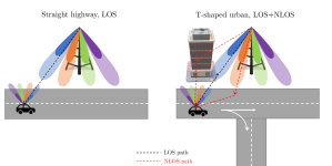
Figure 3: Two UE’s mobility and channel scenarios.

For either scenarios, the ground truth model of beam dynamics $p(\cdot|\cdot)$ is computed from several sequences of SBPIs $S_{0:T}$, by: 1) generating $10^{4}$ UE’s trajectories; 2) for each trajectory, the SBPI sequence $S_{0:T}$ is computed via (4) and (6). Although the Gauss-Markov process exhibits the Markov property on the velocity-position pair $(\upsilon_{t},\omega_{t})$, the SBPI process $\{S_{t},t{\geq}0\}$ is non-Markovian, since $S_{t}$ is a function of the lane and position $\omega_{t}$, and the speed $\upsilon_{t}$ introduces longer-term correlation that cannot be captured by the SBPI transition probability $p(s^{\prime}|s)$. As discussed next, our numerical evaluations reveal that, despite this mismatch, the Markov approximation on $\{S_{t},t{\geq}0\}$ accurately represents the system performance.

The BS and UE use uniform planar arrays with 3D analog beam steering, with codebooks

$$\begin{cases}\mathcal{C}\!\!\!&=\left\{\mathbf{d}_{\rm tx}(\phi^{p}):p=1,\cdots,|\mathcal{C}|\right\},\\ \mathcal{F}\!\!\!&=\left\{\mathbf{d}_{\rm rx}(\theta^{p}):p=1,\cdots,|\mathcal{F}|\right\},\end{cases}$$

where $\theta^{p}$ and $\phi^{p}$ are the $p^{\rm th}$ AoA and AoD directions, respectively, and $\mathbf{d}_{\rm tx}$, $\mathbf{d}_{\rm rx}$ are the associated array response vectors [26]. The set of AoD directions $\{\phi^{p},\forall p\}$ are selected so that beam projections on the road corresponding to the half power bandwidth cover both lanes of the road. The set of AoA directions $\{\theta^{p},\forall p\}$ are selected uniformly spaced in $[0,\pi]^{2}$.

The encoder $q_{\phi}$ of the DR-VAE is a recurrent neural network with one fully-connected hidden layer with 100 units, each with the relu ($\max(0,x)$) activation function. Similarly, the decoder $p_{\boldsymbol{\psi}}$ is a fully-connected feed-forward neural network with two hidden layers, each with 100 units and relu activation. For both encoder and decoder, a softmax layer produces $|\mathcal{S}|$ output units. The DR-VAE is trained online with Algorithm 6: in each training epoch, the DR-VAE is updated using a batch of $N{=}5$ episodes (sampled using either the PBVI or (ER-)MDP policies) and for each episode $N_{\rm trg}{=}6$ trajectories of states are sampled to computed SGA updates; the model of beam dynamics is then updated via SGA and used for the prior belief updates of the next epoch ($5$ episodes), after which the DR-VAE is updated using the new episodes, and so on.

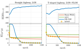
(a) Training progress vs epochs (1 epoch = 5 episodes).

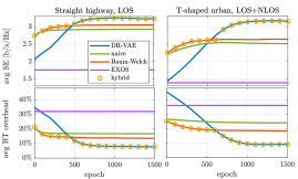
(b) Average spectral efficiency and BT overhead vs epochs.

Figure 4: Training progress of DR-VAE and other algorithms, based on Gauss-Markov mobility and 3D analog beamforming; ${\rm SNR}_{\rm BA}=20$dB.

We use the KL divergence between the ground truth $p(\cdot|\cdot)$ and the learned model of beam dynamics $\hat{p}(\cdot|\cdot)$ to measure the accuracy of the learned model, computed as

$$\overline{\rm KL}(p\|\hat{p})\triangleq\frac{1}{|\mathcal{S}|}\sum_{s\in\mathcal{S}}\sum_{s^{\prime}\in\mathcal{S}\cup\{\bar{s}\}}p(s^{\prime}|s)\ln\frac{p(s^{\prime}|s)}{\hat{p}(s^{\prime}|s)}.$$ (39)

We evaluate the communications performance of a given adaptation policy $\pi$ through the average BT overhead (percentage of the frame duration used for BT) and average spectral efficiency $\bar{\rm SE}^{\pi}$ [bits/s/Hz]. By Little’s law, it is expressed as $\bar{\rm SE}^{\pi}=\frac{\bar{B}_{\rm tot}^{\pi}}{\bar{D}_{\rm tot}W_{\rm tot}},$ where $\bar{B}_{\rm tot}^{\pi}$ is the expected total number of bits successfully delivered to the UE under policy $\pi$ during the episode, and $\bar{D}_{\rm tot}$[s] is the expected episode duration (independent of $\pi$, function only of UE’s mobility).

To evaluate these metrics, we use two types of Monte Carlo simulation approaches:

Markov SBPI with binary SNR model, in which we use the ground truth model of beam dynamics $p(\cdot|\cdot)$ to generate the SBPI sequence, and use the binary SNR model developed in Sec. II-B to assess the learning and communication metrics.

3D analog beamforming model with UE’s mobility, in which UEs’ trajectories and the channel matrix are generated based on either scenario, and the signal model (1) is used to evaluate the beam-training performance and outage conditions. The purpose of this second approach is to validate the modeling abstractions used in our formulation (Markov SBPI dynamics, sectored antenna with binary SNR model).

In addition to the PBVI (Algorithm 1), MDP and ER-MDP policies (Sec. III-B), we simulate two additional policies:

• Exhaustive search over SBPI (EXOS): it is an adaptation of exhaustive search proposed in [36]; however, unlike [36], which sweeps the entire AoA and AoD range (in our setting, a total of $|\mathcal{C}|\cdot|\mathcal{F}|=512$ beam pairs, unfeasible within the frame duration), we restrict the exhaustive search to the SBPIs only (i.e., those beam pairs that maximize the beamforming gain within the coverage area of the BS, see (7)). These represent a much smaller set of 15 beam pairs for the straight highway, LOS scenario and 17 beam pairs for the T-shaped urban, LOS+NLOS scenario. Note that no training is required for EXOS since it does not utilize the estimated beam dynamics.

• Short-timescale single-shot (STSS) policy [12]: it is a state-of-the-art POMDP policy with a single-shot beam training phase of fixed duration. Note that [12] assumes prior knowledge of the SBPI transition model; we use both the ground truth and the DR-VAE estimated models to evaluate STSS.

V-B Model training performance

In Fig. 4(a) and Fig. 4(b), we show the training progress of DR-VAE in terms of average ELBO, KL divergence, spectral efficiency and BT overhead, based on the Gauss-Markov mobility and 3D analog beamforming, for both scenarios. We compare different frameworks: the proposed DR-VAE (Algorithm 6), the naive approach (see (15)) and the Baum-Welch algorithm [11]. Observations are sampled following the PBVI-based policy (Algorithm 1). We note that, as training progresses, the ELBO increases and $\overline{\rm KL}(p\|\hat{p})$ decreases simultaneously, indicating an improvement in the accuracy of the learned transition model. At the same time, the average spectral efficiency increases and the BT overhead decreases, indicating that the POMDP adaptation framework uses resources more efficiently by leveraging an accurate model of beam dynamics. Notably, thanks to its error robustness, the PBVI policy yields better spectral efficiency than EXOS, even in the early training epochs, demonstrating that it provides a satisfactory baseline performance even with inaccurate models of beam dynamics; as learning progresses, its performance improves even further.
Comparing the two scenarios, we observe a slight performance degradation in the T-shaped urban, LOS+NLOS scenario, attributed to NLOS channel components causing more frequent BT feedback errors (as also reflected by the increased misalignment to alignment gain ratio $\rho$, see Table 1).

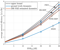
(a) Straight highway, LOS scenario

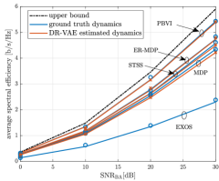
(b) T-shaped urban, LOS+NLOS scenario

Figure 5: Average spectral efficiency versus SNR. Monte Carlo simulation based on Markov SBPI with binary SNR model (solid lines) and 3D analog beamforming model with UE’s mobility (markers).

(a) Average spectral efficiency versus $\rho$.

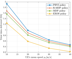
(b) Total data delivered vs mean speed $\mu_{v}$; ${\rm SNR}_{\rm BA}=20$dB, $\rho=-10$dB.

Figure 6: Monte-Carlo simulations based on: Markov SBPI with binary SNR model; ground truth model of beam dynamics; straight highway, LOS scenario.

Comparing DR-VAE with other algorithms, we note that Baum-Welch and the naive approach converge faster initially, but get stuck at a suboptimal point as training progresses: upon reaching convergence, DR-VAE offers ${\sim}90\%$ (straight highway, LOS) and ${\sim}95\%$ (T-shaped urban, LOS+NLOS) reduction in KL divergence compared to the other two methods. This improved accuracy translates into a ${\sim}10\%$ and ${\sim}20\%$ spectral efficiency gain in the two scenarios, respectively, and ${\sim}50\%$ reduction of BT overhead, as depicted in the figure. Motivated by the improved early convergence of Baum-Welch, we propose a hybrid approach: in the early learning stages, the POMDP adaptation framework uses the prior beliefs generated based on the model learned by the Baum-Welch algorithm; when the ELBO metric converges, it switches to the model provided by the DR-VAE. Such a hybrid scheme is possible thanks to the decoupling of policy design and learning of beam dynamics via the dual timescale approach: we can thus train multiple models of beam dynamics simultaneously and use the prior belief generated based on any one model. As can be seen in the figure (markers), this hybrid approach achieves the best performance across all metrics.

V-C Spectral Efficiency

In Fig. 5(a) and 5(b), we present the spectral efficiency performance as a function of the target SNR for the two scenarios, using Monte-Carlo simulation over $10^{5}$ episodes. In addition to the three proposed policies (PBVI, MDP and ER-MDP policies), the state-of-the-art STSS [12] and EXOS, we also evaluate a genie-aided upper bound, computed using error-free BT feedback and knowledge of the ground truth model of beam dynamics. Note that this upper bound is not attainable in practice, due to feedback errors and inaccuracies in the learned model. To assess the impact of the DR-VAE learning algorithm on performance, all these schemes (except EXOS and the upper bound) are evaluated using both the DR-VAE estimated model of beam dynamics for the belief updates, computed after convergence of the learning algorithm (red curves), and also using the ground truth model of beam dynamics (blue curves).

We observe that, for all the schemes, the DR-VAE performs very close to the counterpart using the ground-truth model of beam dynamics, thus confirming the results of Fig. 4(a) and Fig. 4(b). The PBVI policy coupled with DR-VAE yields the best performance, close to the genie-aided upper bound. For the straight highway, LOS scenario, it outperforms the ER-MDP, STSS/MDP (shown together since they exhibit nearly identical performance), and EXOS by up to $8\%$, $16\%$ and $85\%$ in spectral efficiency, respectively. For the T-shaped urban, LOS+NLOS scenario, PBVI (coupled with DR-VAE) shows even bigger gains: it outperforms ER-MDP, STSS, MDP, and EXOS by up to $14\%$, $20\%$, $28\%$ and $130\%$ in spectral efficiency, respectively.

The gain of PBVI over the other policies is attributed to its enhanced robustness against feedback errors, incorporated via the BT feedback distribution, and its optimized and adaptive BT design. Although ER-MDP suffers from a slight performance degradation with respect to PBVI, it outperforms all other schemes: unlike the MDP-based policy, ER-MDP incorporates error-robustness by using POMDP belief updates, and unlike STSS that uses a fixed BT duration, ER-MDP adjusts the BT overhead adaptively by leveraging the BT feedback. This is a remarkable result given that ER-MDP is a low-complexity policy, compared to the POMDP-based STSS.

To assess the validity of the modeling abstractions, we also evaluate the performance based on the Markov SBPI with binary SNR model (solid lines) and the 3D analog beamforming model with UE’s mobility (markers). It can be seen that the values under the two approaches match, thereby verifying the accuracy of the proposed modeling abstractions.
In Fig. 6(a), we depict the spectral efficiency vs the misalignment to alignment gain ratio $\rho$ for the straight highway, LOS scenario, under the Markov SBPI with binary SNR model. We use the ground truth model for this evaluation, since our previous results demonstrated that DR-VAE learns the model accurately. Note that larger values of $\rho$ account for the effect of more severe NLOS multipath and sidelobes, causing more frequent feedback errors. As expected, the performance of the four policies degrades as $\rho$ increases. Yet, notably, PBVI degrades the least thanks to its robustness to errors, whereas EXOS degrades the most. Moreover, for small to medium values of $\rho$, ER-MDP performs very close to PBVI, since feedback errors become less frequent. At the same time, we found that the total optimization and execution time of ER-MDP is ${\sim}5$ times smaller than PBVI, so that ER-MDP offers a low-complexity alternative to PBVI for small values of $\rho$.
In Fig. 6(b), we depict the average total data delivered to the UE successfully as a function of the mean UE speed $\mu_{v}$. We note a monotonically decreasing trend with the mean speed $\mu_{v}$, attributed to the shorter average episode duration as speed increases, and the exacerbated overhead of BT since SBPIs change more frequently. The behavior is in line with what we observed previously: PBVI outperforms ER-MDP and MDP-based policies, which in turn outperform EXOS.

VI Conclusion and Future Work

This paper proposed a dual timescale learning and adaptation framework, in which the beam dynamics are learned to enable predictive beam-tracking, and then exploited to design adaptive beam-training policies. In the short-timescale, we developed a POMDP framework to design an approximately optimal policy. In the long-timescale, we designed a deep recurrent variational autoencoder-based learning framework, which uses noisy observations collected under the policy to learn a transition model of beam dynamics. Via simulation, we demonstrated the superior learning performance of the proposed learning framework over the Baum-Welch algorithm and a naive learning method, with spectral efficiency gains of $\sim 10\%$ and reduced beam-training overhead by $\sim 50\%$. Our performance evaluation demonstrated that the proposed policy, coupled with the learning framework, yields near-optimal performance, with ${\sim}16\%$ spectral efficiency gains over a state-of-the-art POMDP policy. This work paves the way to future research on beam tracking design in multi-base station and multi-user settings, by learning and leveraging the joint beam dynamics of multiple users, as well as the extension to hybrid beamforming architectures.

Appendix A: Proof of Theorem 1

Proof.

We use induction to prove P1. P1 holds for $k{=}K$ since $\mathcal{Q}_{K}{=}\{\mathbf{0}\}{=}\mathcal{P}(\mathbf{0})$. Assume $\mathcal{Q}_{j}$ satisfies P1 for $j{>}k$, for some $k{\in}\mathcal{K}$. We show that it implies $\mathcal{Q}_{k}$ satisfies P1 as well. Let $\boldsymbol{\alpha}{\in}\mathcal{Q}_{k}$, with $\mathcal{Q}_{k}$ given by (20). If $\boldsymbol{\alpha}{=}{\rm SE}_{\rm BA}{\cdot}\left(1-\frac{k}{K}\right)\mathbf{e}_{\ell}$, then $\mathcal{P}(\boldsymbol{\alpha})=\cup_{i=1}^{|\mathcal{S}|}\{{\rm SE}_{\rm BA}{\cdot}(1-k/K)\mathbf{e}_{i}\}\subseteq\mathcal{Q}_{k}.$ Now, consider ${\boldsymbol{\alpha}}{=}\sum_{y\in\mathcal{Y}}\mathbb{P}_{Y}(y|\cdot,{\mathcal{S}}_{\rm BT}){\odot}{\boldsymbol{\alpha}}^{(y)}$, for some $[\boldsymbol{\alpha}^{(y)}]_{y\in\mathcal{Y}}\in\mathcal{Q}_{k+n+1}^{n+1}$ and ${\mathcal{S}}_{\rm BT}\in\mathcal{A}_{{\rm BT},k}$ with $|{\mathcal{S}}_{\rm BT}|=n$, so that $\boldsymbol{\alpha}\in\mathcal{Q}_{k}$. Let ${\rm prm}(\cdot)$ be a generic permutation operator, and $\tilde{\boldsymbol{\alpha}}{\triangleq}{\rm prm}(\boldsymbol{\alpha}){\in}\mathcal{P}(\boldsymbol{\alpha})$. We will show that $\tilde{\boldsymbol{\alpha}}{\in}\mathcal{Q}_{k}$, hence $\mathcal{P}(\boldsymbol{\alpha})\subseteq\mathcal{Q}_{k}$, which proves the induction step and P1.

To prove $\tilde{\boldsymbol{\alpha}}{\in}\mathcal{Q}_{k}$, we need to show that there is a BT action over the BPI set $\tilde{\mathcal{S}}_{\rm BT}{\in}\mathcal{A}_{{\rm BT},k}$ and vectors $[\tilde{\boldsymbol{\alpha}}^{(\tilde{y})}]_{\tilde{y}\in\tilde{\mathcal{Y}}}{\in}\mathcal{Q}_{k+n+1}^{n+1}$ such that $\tilde{\boldsymbol{\alpha}}{=}\sum_{\tilde{y}\in\tilde{\mathcal{Y}}}\mathbb{P}_{Y}(\tilde{y}|\cdot,\tilde{\mathcal{S}}_{\rm BT}){\odot}\tilde{\boldsymbol{\alpha}}^{(\tilde{y})}$, where $\tilde{\mathcal{Y}}{\equiv}\tilde{\mathcal{S}}_{\rm BT}{\cup}\{0\}$ is the corresponding observation set. Let $\chi{:}\mathcal{S}{\mapsto}\mathcal{S}$ be the function that maps a state $s$ to its permuted state $s^{\prime}{=}\chi(s)$ through the operator ${\rm prm}(\cdot)$, and let $\Lambda(\cdot)$ be the inverse mapping ($s{=}\Lambda(s^{\prime})$), so that for $\tilde{\mathbf{a}}{=}{\rm prm}(\mathbf{a})$ we have $\tilde{\mathbf{a}}(\chi(s)){=}\mathbf{a}(s)$ and $\tilde{\mathbf{a}}(s){=}\mathbf{a}(\Lambda(s))$. We define the new BT set $\tilde{\mathcal{S}}_{\rm BT}{=}\{\chi(s){:}s{\in}{\mathcal{S}}_{\rm BT}\}$ and new vectors $\tilde{\boldsymbol{\alpha}}^{(0)}{=}{\rm prm}({\boldsymbol{\alpha}}^{(0)})$, $\tilde{\boldsymbol{\alpha}}^{(\chi(y))}{=}{\rm prm}({\boldsymbol{\alpha}}^{(y)}),\forall y{\in}{\mathcal{S}}_{\rm BT}$. Clearly, $\tilde{\boldsymbol{\alpha}}^{(\tilde{y})}{\in}\mathcal{Q}_{k+n+1},\forall\tilde{y}{\in}\tilde{\mathcal{Y}}$, from the induction hypothesis, and $\tilde{\mathcal{S}}_{\rm BT}{\in}\mathcal{A}_{{\rm BT},k}$, hence $\sum_{\tilde{y}\in\tilde{\mathcal{Y}}}\mathbb{P}_{Y}(\tilde{y}|\cdot,\tilde{\mathcal{S}}_{\rm BT}){\odot}\tilde{\boldsymbol{\alpha}}^{(\tilde{y})}{\in}\mathcal{Q}_{k}$. It remains to prove that $\tilde{\boldsymbol{\alpha}}{=}\sum_{\tilde{y}\in\tilde{\mathcal{Y}}}\mathbb{P}_{Y}(\tilde{y}|\cdot,\tilde{\mathcal{S}}_{\rm BT}){\odot}\tilde{\boldsymbol{\alpha}}^{(\tilde{y})}$, i.e., $\sum_{\tilde{y}\in\tilde{\mathcal{Y}}}\mathbb{P}_{Y}(\tilde{y}|s,\tilde{\mathcal{S}}_{\rm BT})\tilde{\boldsymbol{\alpha}}^{(\tilde{y})}(s){=}\boldsymbol{\alpha}(\Lambda(s)),\forall s$, since $\tilde{\boldsymbol{\alpha}}{=}{\rm prm}(\boldsymbol{\alpha})$. In fact, $\forall s\in\mathcal{S}$, and letting $\Lambda(0)=\chi(0)=0$,

$$\sum_{\tilde{y}\in\tilde{\mathcal{Y}}}\mathbb{P}_{Y}(\tilde{y}|s,\tilde{\mathcal{S}}_{\rm BT})\tilde{\boldsymbol{\alpha}}^{(\tilde{y})}(s)\stackrel{{\scriptstyle(a)}}{{=}}\sum_{\tilde{y}\in\tilde{\mathcal{Y}}}\mathbb{P}_{Y}(\tilde{y}|s,\tilde{\mathcal{S}}_{\rm BT}){\boldsymbol{\alpha}}^{(\Lambda(\tilde{y}))}(\Lambda(s))$$

$$\stackrel{{\scriptstyle(b)}}{{=}}\sum_{y\in{\mathcal{S}}_{\rm BT}\cup\{0\}}\underbrace{\mathbb{P}_{Y}(\chi(y)|s,\tilde{\mathcal{S}}_{\rm BT})}_{\stackrel{{\scriptstyle(c)}}{{=}}\mathbb{P}_{Y}(y|\Lambda(s),{\mathcal{S}}_{\rm BT})}{\boldsymbol{\alpha}}^{(y)}(\Lambda(s))\stackrel{{\scriptstyle(d)}}{{=}}\boldsymbol{\alpha}(\Lambda(s)),$$

where (a) follows from the definition of $\tilde{\boldsymbol{\alpha}}^{(\tilde{y})}$; (b) from $\tilde{\mathcal{S}}_{\rm BT}=\{\chi(y):y{\in}{\mathcal{S}}_{\rm BT}\}$ and $\Lambda(\chi(y)){=}y$; (c) from the symmetry in the observation model; (d) by inspection. P1 is thus proved.

P1 implies that $\mathcal{Q}_{k}{\equiv}\cup_{\boldsymbol{\alpha}\in\mathcal{Q}_{k}^{\rm sort}}\mathcal{P}(\boldsymbol{\alpha})$. P2 then follows since $V_{k}^{*}(\boldsymbol{\beta}){=}\max\limits_{\boldsymbol{\alpha}\in\mathcal{Q}_{k}^{\rm sort}}\max\limits_{\tilde{\boldsymbol{\alpha}}\in\mathcal{P}(\boldsymbol{\alpha})}\langle\boldsymbol{\beta},\tilde{\boldsymbol{\alpha}}\rangle=\max\limits_{\boldsymbol{\alpha}\in\mathcal{Q}_{k}^{\rm sort}}\langle\mathrm{sort}(\boldsymbol{\beta}),\boldsymbol{\alpha}\rangle$ and $\mathrm{sort}(\boldsymbol{\beta}^{\prime}){=}\mathrm{sort}(\boldsymbol{\beta}),\forall\boldsymbol{\beta}^{\prime}{\in}\mathcal{P}(\boldsymbol{\beta})$. ∎

Appendix B: Proof of Theorem 2

Proof.

We prove the theorem by induction. P1-P4 hold trivially for $k{=}K$ since $V_{K}^{*}(\mathcal{U}){=}0$. Assume P1-P4 hold for $j{>}k$, for some $k{<}K$. We will prove they hold for $k$ as well.

P1: when $\mathcal{U}{=}\{s\}$, using the induction hypothesis P1 we obtain $V_{k}^{(\mathrm{BT})}(\{s\},{\mathcal{S}}_{\rm BT}){=}{\rm SE}_{\rm BA}{\cdot}[1{-}(k{+}1)/K]<V_{k}^{(\mathrm{DC})}(\{s\}){=}{\rm SE}_{\rm BA}{\cdot}(1{-}k/K)$. Hence, the optimal action is DC with value $V_{k}^{*}(\{s\})={\rm SE}_{\rm BA}{\cdot}(1-k/K)$.

P2: $V_{k}^{*}(\mathcal{U}){\geq}V_{k+1}^{*}(\mathcal{U})$ follows from the value iteration algorithm, since $1{-}k/K{>}1{-}(k{+}1)/K$, $\mathcal{A}_{{\rm BT},k}{\supseteq}\mathcal{A}_{{\rm BT},k+1}$, and $V_{k+|{\mathcal{S}}_{\rm BT}|+1}^{*}(\mathcal{U}){\geq}V_{k{+}1{+}|{\mathcal{S}}_{\rm BT}|{+}1}^{*}(\mathcal{U})$ (induction hypothesis).

P3: consider ${\mathcal{S}}_{{\rm BT}}^{(0)}$ such that $|{\mathcal{S}}_{{\rm BT}}^{(0)}{\setminus}\mathcal{U}|{\geq}1$, and a new BT set ${\mathcal{S}}_{{\rm BT}}^{(1)}{=}{\mathcal{S}}_{{\rm BT}}^{(0)}{\cap}\mathcal{U}$. Since $\mathcal{U}{\cap}{\mathcal{S}}_{{\rm BT}}^{(0)}{=}\mathcal{U}{\cap}{\mathcal{S}}_{{\rm BT}}^{(1)}$, and $\mathcal{U}{\setminus}{\mathcal{S}}_{{\rm BT}}^{(0)}{=}\mathcal{U}{\setminus}{\mathcal{S}}_{{\rm BT}}^{(1)}$, P2 and $|{\mathcal{S}}_{{\rm BT}}^{(1)}|{<}|{\mathcal{S}}_{{\rm BT}}^{(0)}|$ imply suboptimality of ${\mathcal{S}}_{{\rm BT}}^{(0)}$.

P4: consider $\mathcal{U}{\equiv}\{s_{1},s_{2},{\cdots},s_{|\mathcal{U}|}\}$ with $|\mathcal{U}|{\geq}2$, and a BT set ${\mathcal{S}}_{{\rm BT}}^{(1)}{=}\{s_{1},s_{2},{\cdots},s_{n}\}{\subset}\mathcal{U}$. Without loss of generality, assume that $\boldsymbol{\beta}(s_{1}){\geq}\boldsymbol{\beta}(s_{2}){\geq}\dots\boldsymbol{\beta}(s_{n})$, $\boldsymbol{\beta}(s_{n+1}){>}\boldsymbol{\beta}(s_{n})$ and $\boldsymbol{\beta}(s_{n+1}){\geq}\boldsymbol{\beta}(s_{n+2}){\geq}\dots\boldsymbol{\beta}(s_{|\mathcal{U}|})$; in other words, ${\mathcal{S}}_{{\rm BT}}^{(1)}$ does not scan the $n$ most likely BPIs, since $\boldsymbol{\beta}(s_{n+1}){>}\boldsymbol{\beta}(s_{n})$. Let a new set ${\mathcal{S}}_{{\rm BT}}^{(0)}{=}\{s_{1},s_{2},\cdots,s_{n-1}\}{\cup}\{s_{n+1}\}{\subset}\mathcal{U}$, which scans the more likely $s_{n+1}$ rather than $s_{n}$. We want to show that $V_{k}^{(\mathrm{BT})}(\mathcal{U},{\mathcal{S}}_{{\rm BT}}^{(0)}){\geq}V_{k}^{(\mathrm{BT})}(\mathcal{U},{\mathcal{S}}_{{\rm BT}}^{(1)})$, i.e., ${\mathcal{S}}_{{\rm BT}}^{(1)}$ is suboptimal. Using $\mathcal{U}{\cap}{\mathcal{S}}_{{\rm BT}}^{(i)}{\equiv}{\mathcal{S}}_{{\rm BT}}^{(i)}$, $\mathcal{U}{\setminus}{\mathcal{S}}_{{\rm BT}}^{(i)}{\equiv}\{s_{n+i}\}\cup\{s_{n+2},\dots,s_{|\mathcal{U}|}\}{\triangleq}\mathcal{U}^{(i)}$, and the induction hypothesis P1, we obtain

$$V_{k}^{(\mathrm{BT})}(\mathcal{U},{\mathcal{S}}_{{\rm BT}}^{(i)})= \frac{\sum_{s\in{\mathcal{S}}_{{\rm BT}}^{(i)}}\boldsymbol{\beta}(s)}{\sum_{s\in\mathcal{U}}\boldsymbol{\beta}(s)}{\rm SE}_{\rm BA}{\cdot}\Big{(}1{-}\frac{k{+}n{+}1}{K}\Big{)}$$

$$+\frac{\sum_{s\in\mathcal{U}^{(i)}}\boldsymbol{\beta}(s)}{\sum_{s\in\mathcal{U}}\boldsymbol{\beta}(s)}V_{k+n+1}^{*}(\mathcal{U}^{(i)}).$$ (40)

Now, consider $V_{k+n+1}^{*}(\mathcal{U}^{(1)})$. If it is optimized by DC, then

$$V_{k{+}n{+}1}^{*}(\mathcal{U}^{(1)}){=}V_{k{+}n{+}1}^{(\mathrm{DC})}(\mathcal{U}^{(1)}){=}\frac{\boldsymbol{\beta}(s_{n{+}1})}{\!\!\!\sum\limits_{s\in\mathcal{U}^{(1)}}\!\!\!\boldsymbol{\beta}(s)}{\rm SE}_{\rm BA}\Big{(}\!1{-}\frac{k{+}n{+}1}{K}\!\Big{)}\!,$$

$$V_{k+n+1}^{*}(\mathcal{U}^{(0)}){\geq}V_{k{+}n{+}1}^{(\mathrm{DC})}(\mathcal{U}^{(0)}){\geq}\frac{\boldsymbol{\beta}(s_{n})}{\!\!\!\!\sum\limits_{s\in\mathcal{U}^{(0)}}\boldsymbol{\beta}(s)}{\rm SE}_{\rm BA}\Big{(}\!1{-}\frac{k{+}n{+}1}{K}\!\Big{)}\!,$$

where we used $\max\limits_{s\in\mathcal{U}^{(1)}}\boldsymbol{\beta}(s){=}\boldsymbol{\beta}(s_{n+1})$ and $\max\limits_{s\in\mathcal{U}^{(0)}}\boldsymbol{\beta}(s){\geq}\boldsymbol{\beta}(s_{n})$; the inequality holds since choosing DC may be suboptimal for $V_{k+n+1}^{*}(\mathcal{U}^{(0)})$. Hence, $V_{k}^{(\mathrm{BT})}(\mathcal{U},{\mathcal{S}}_{{\rm BT}}^{(0)})-V_{k}^{(\mathrm{BT})}(\mathcal{U},{\mathcal{S}}_{{\rm BT}}^{(1)})\geq 0$.

Now, consider the case when $V_{k+n+1}^{*}(\mathcal{U}^{(1)})$ is optimized by the BT action over the BPI set $\mathcal{S}_{{\rm BT}}^{(1)}{\equiv}\{s_{n+1},\dots,s_{n+m}\}$ (from the induction hypothesis P4, choosing the $m$ most likely BPIs is optimal), and let $\mathcal{S}_{{\rm BT}}^{(0)}{\equiv}\{s_{n}\}{\cup}\{s_{n+2},\cdots,s_{n+m}\}$. Since $\mathcal{U}^{(i)}{\cap}{\mathcal{S}}_{{\rm BT}}^{(i)}{\equiv}{\mathcal{S}}_{{\rm BT}}^{(i)}$, $\mathcal{U}^{(1)}{\setminus}{\mathcal{S}}_{{\rm BT}}^{(1)}{\equiv}\mathcal{U}^{(0)}{\setminus}{\mathcal{S}}_{{\rm BT}}^{(0)}{\triangleq}\mathcal{U}^{(2)}$, it follows

$$V_{k+n+1}^{*}(\mathcal{U}^{(i)}){\geq}V_{k{+}n{+}1}^{(\mathrm{BT})}(\mathcal{U}^{(i)},{\mathcal{S}}_{{\rm BT}}^{(i)}){=}\frac{\sum_{s\in\mathcal{U}^{(2)}}\boldsymbol{\beta}(s)}{\sum_{s\in\mathcal{U}^{(i)}}\boldsymbol{\beta}(s)}$$

$${\times}V_{k+n+m+2}^{*}(\mathcal{U}^{(2)}){+}\frac{\sum_{s\in{\mathcal{S}}_{{\rm BT}}^{(i)}}\boldsymbol{\beta}(s)}{\sum_{s\in\mathcal{U}^{(i)}}\boldsymbol{\beta}(s)}{\rm SE}_{\rm BA}{\cdot}\left(\!1{-}\frac{k{+}n{+}m{+}2}{K}\!\right)\!,$$

with equality for $i{=}1$ (since $V_{k+n+1}^{*}(\mathcal{U}^{(1)})$ is optimized by BT over the set $\mathcal{S}_{{\rm BT}}^{(1)}$), and the inequality for $i{=}0$ holds since choosing BT with set ${\mathcal{S}}_{{\rm BT}}^{(0)}$ may be suboptimal for $V_{k+n+1}^{*}(\mathcal{U}^{(0)})$. Using the fact that $\boldsymbol{\beta}(s_{n+1}){-}\boldsymbol{\beta}(s_{n}){>}0$, it follows that $V_{k}^{(\mathrm{BT})}(\mathcal{U},{\mathcal{S}}_{{\rm BT}}^{(0)}){\geq}V_{k}^{(\mathrm{BT})}(\mathcal{U},{\mathcal{S}}_{{\rm BT}}^{(1)})$, and ${\mathcal{S}}_{{\rm BT}}^{(1)}$ is suboptimal. The induction step, hence the theorem, are proved. ∎

Muddassar Hussain received the Bachelors in electrical engineering from National University of Sciences and Technology (NUST), Islamabad, Pakistan, in 2013. He received the Master’s and PhD degrees in electrical and computer engineering from Purdue University, West Lafayette, IN, USA, in 2019 and 2021, respectively. Currently, he is a senior systems engineer at Qualcomm Technologies. His research interest lie in the areas of optimization algorithms design, stochastic optimal control, machine learning and reinforcement learning with applications to 5G wireless communication system design. He is reviewer of several IEEE journals and conferences, including IEEE Transactions on Wireless Communications, IEEE Transactions on Signal Processing, IEEE Transactions on Vehicular Technologies, IEEE Globecom, IEEE ICC.

Nicolò Michelusi (Senior Member, IEEE) received the B.Sc. (with honors), M.Sc. (with honors), and Ph.D. degrees from the University of Padova, Italy, in 2006, 2009, and 2013, respectively, and the M.Sc. degree in telecommunications engineering from the Technical University of Denmark, Denmark, in 2009, as part of the T.I.M.E. double degree program. From 2013 to 2015, he was a Postdoctoral Research Fellow with the Ming-Hsieh Department of Electrical Engineering, University of Southern California, Los Angeles, CA, USA, and from 2016 to 2020, he was an Assistant Professor with the School of Electrical and Computer Engineering, Purdue University, West Lafayette, IN, USA. He is currently an Assistant Professor with the School of Electrical, Computer and Energy Engineering, Arizona State University, Tempe, AZ, USA. His research interests include 5G wireless networks, millimeter-wave communications, stochastic optimization, distributed optimization, and federated learning over wireless. He is currently an Associate Editor for the IEEE TRANSACTIONS ON WIRELESS COMMUNICATIONS, and a Reviewer for several IEEE journals. He was the Co-Chair for the Distributed Machine Learning and Fog Network workshop at the IEEE INFOCOM 2021, the Wireless Communications Symposium at the IEEE Globecom 2020, the IoT, M2M, Sensor Networks, and Ad-Hoc Networking track at the IEEE VTC 2020, and the Cognitive Computing and Networking symposium at the ICNC 2018. He received the NSF CAREER award in 2021.

References

• [1] M. Hussain and N. Michelusi, “Adaptive Beam Alignment in Mm-Wave Networks: A Deep Variational Autoencoder Architecture,” in IEEE Globecom, 2021, to appear.
• [2] J. Choi, V. Va, N. Gonzalez-Prelcic, R. Daniels, C. R. Bhat, and R. W. Heath, “Millimeter-wave vehicular communication to support massive automotive sensing,” IEEE Communications Magazine, vol. 54, no. 12, pp. 160–167, 2016.
• [3] T. S. Rappaport, R. W. Heath, R. C. Daniels, and J. N. Murdock, Millimeter wave wireless communications.   Prentice Hall, 2015.
• [4] M. Giordani, A. Zanella, and M. Zorzi, “Millimeter wave communication in vehicular networks: Challenges and opportunities,” in 6th International Conference on Modern Circuits and Systems Technologies.   IEEE, 2017, pp. 1–6.
• [5] V. Va, T. Shimizu, G. Bansal, and R. W. Heath, “Beam design for beam switching based millimeter wave vehicle-to-infrastructure communications,” in IEEE ICC, 2016, pp. 1–6.
• [6] M. Scalabrin, N. Michelusi, and M. Rossi, “Beam training and data transmission optimization in millimeter-wave vehicular networks,” in IEEE Globecom, Dec 2018, pp. 1–7.
• [7] M. Hussain, M. Scalabrin, M. Rossi, and N. Michelusi, “Mobility and blockage-aware communications in millimeter-wave vehicular networks,” IEEE Transactions on Vehicular Technology, vol. 69, no. 11, pp. 13 072–13 086, 2020.
• [8] S.-E. Chiu, N. Ronquillo, and T. Javidi, “Active Learning and CSI Acquisition for mmWave Initial Alignment,” IEEE Journal on Selected Areas in Communications, vol. 37, no. 11, pp. 2474–2489, 2019.
• [9] M. Hussain and N. Michelusi, “Energy-Efficient Interactive Beam Alignment for Millimeter-Wave Networks,” IEEE Transactions on Wireless Communications, vol. 18, no. 2, pp. 838–851, Feb 2019.
• [10] J. Chung, K. Kastner, L. Dinh, K. Goel, A. C. Courville, and Y. Bengio, “A recurrent latent variable model for sequential data,” in Advances in Neural Information Processing Systems, vol. 28, 2015.
• [11] L. R. Rabiner, “A tutorial on hidden Markov models and selected applications in speech recognition,” Proceedings of the IEEE, vol. 77, no. 2, pp. 257–286, 1989.
• [12] J. Seo, Y. Sung, G. Lee, and D. Kim, “Training Beam Sequence Design for Millimeter-Wave MIMO Systems: A POMDP Framework,” IEEE Transactions on Signal Processing, vol. 64, no. 5, pp. 1228–1242, 2016.
• [13] N. Michelusi and M. Hussain, “Optimal beam-sweeping and communication in mobile millimeter-wave networks,” in IEEE International Conference on Communications (ICC), May 2018, pp. 1–6.
• [14] Z. Marzi, D. Ramasamy, and U. Madhow, “Compressive Channel Estimation and Tracking for Large Arrays in mm-Wave Picocells,” IEEE Journal of Selected Topics in Signal Processing, vol. 10, no. 3, pp. 514–527, April 2016.
• [15] V. Va, J. Choi, T. Shimizu, G. Bansal, and R. W. Heath, “Inverse Multipath Fingerprinting for Millimeter Wave V2I Beam Alignment,” IEEE Transactions on Vehicular Technology, vol. 67, no. 5, pp. 4042–4058, May 2018.
• [16] T.-H. Chou, N. Michelusi, D. J. Love, and J. V. Krogmeier, “Fast Position-Aided MIMO Beam Training via Noisy Tensor Completion,” IEEE Journal of Selected Topics in Signal Processing, vol. 15, no. 3, pp. 774–788, 2021.
• [17] Y. Heng and J. G. Andrews, “Machine Learning-Assisted Beam Alignment for mmWave Systems,” in IEEE Global Communications Conference (GLOBECOM), 2019, pp. 1–6.
• [18] V. Va, T. Shimizu, G. Bansal, and R. W. Heath, “Online learning for position-aided millimeter wave beam training,” IEEE Access, vol. 7, pp. 30 507–30 526, 2019.
• [19] N. Gonzalez-Prelcic, R. Mendez-Rial, and R. W. Heath, “Radar aided beam alignment in MmWave V2I communications supporting antenna diversity,” in Information Theory and Applications Workshop (ITA), Jan 2016, pp. 1–7.
• [20] A. Ali, N. Gonzalez-Prelcic, and R. W. Heath, “Millimeter wave beam-selection using out-of-band spatial information,” IEEE Transactions on Wireless Communications, vol. 17, no. 2, pp. 1038–1052, 2018.
• [21] A. Alkhateeb, S. Alex, P. Varkey, Y. Li, Q. Qu, and D. Tujkovic, “Deep learning coordinated beamforming for highly-mobile millimeter wave systems,” IEEE Access, vol. 6, pp. 37 328–37 348, 2018.
• [22] M. Hussain and N. Michelusi, “Second-best beam-alignment via bayesian multi-armed bandits,” in IEEE Global Communications Conference (GLOBECOM), 2019, pp. 1–6.
• [23] Y. Wang, N. J. Myers, N. González-Prelcic, and R. W. Heath, “Deep Learning-based Compressive Beam Alignment in mmWave Vehicular Systems,” arXiv preprint arXiv:2103.00125, 2021.
• [24] V. Va, J. Choi, and R. W. Heath, “The impact of beamwidth on temporal channel variation in vehicular channels and its implications,” IEEE Transactions on Vehicular Technology, vol. 66, no. 6, pp. 5014–5029, June 2017.
• [25] T. Bai and R. W. Heath, “Coverage analysis for millimeter wave cellular networks with blockage effects,” in IEEE Global Conference on Signal and Information Processing, Dec 2013, pp. 727–730.
• [26] A. Alkhateeb, O. El Ayach, G. Leus, and R. W. Heath, “Channel estimation and hybrid precoding for millimeter wave cellular systems,” IEEE Journal of Selected Topics in Signal Processing, vol. 8, no. 5, pp. 831–846, 2014.
• [27] M. R. Akdeniz, Y. Liu, M. K. Samimi, S. Sun, S. Rangan, T. S. Rappaport, and E. Erkip, “Millimeter Wave Channel Modeling and Cellular Capacity Evaluation,” IEEE Journal on Selected Areas in Communications, vol. 32, no. 6, pp. 1164–1179, June 2014.
• [28] A. Lozano, “Long-term transmit beamforming for wireless multicasting,” in IEEE International Conference on Acoustics, Speech and Signal Processing - ICASSP ’07, vol. 3, 2007, pp. III–417–III–420.
• [29] V. Krishnamurthy, Partially observed Markov decision processes.   Cambridge university press, 2016.
• [30] J. Pineau, G. Gordon, and S. Thrun, “Anytime Point-based Approximations for Large POMDPs,” J. Artif. Int. Res., vol. 27, no. 1, pp. 335–380, Nov. 2006.
• [31] D. P. Kingma and M. Welling, “An introduction to variational autoencoders,” Foundations and Trends in Machine Learning, vol. 12, no. 4, pp. 307–392, 2019.
• [32] E. Jang, S. Gu, and B. Poole, “Categorical Reparameterization with Gumbel-Softmax,” in ICLR, 2017.
• [33] H. Tabassum, M. Salehi, and E. Hossain, “Fundamentals of mobility-aware performance characterization of cellular networks: A tutorial,” IEEE Communications Surveys Tutorials, vol. 21, no. 3, pp. 2288–2308, 2019.
• [34] J. Xu, Y. Zhao, and X. Zhu, “Mobility model based handover algorithm in LTE-Advanced,” in 10th International Conference on Natural Computation (ICNC), 2014, pp. 230–234.
• [35] I. Khan, G. Hoang, and J. Harri, “Rethinking cooperative awareness for future V2X safety-critical applications,” in IEEE Vehicular Networking Conference (VNC), 2017, pp. 73–76.
• [36] C. Jeong, J. Park, and H. Yu, “Random access in millimeter-wave beamforming cellular networks: issues and approaches,” IEEE Communications Magazine, vol. 53, no. 1, pp. 180–185, January 2015.