Evolution of the Andreev bands in the half-filled superconducting periodic Anderson model

Abstract

We employ the periodic Anderson model with superconducting correlations in the conduction band at half filling to study the behavior of the in-gap bands in a heterostructure consisting of a molecular layer deposited on the surface of a conventional superconductor. We use the dynamical mean-field theory to map the lattice model on the superconducting single impurity model with self-consistently determined bath and use the continuous-time hybridization expansion (CT-HYB) quantum Monte Carlo and the iterative perturbation theory (IPT) as solvers for the impurity problem. We present phase diagrams for square and triangular lattice that both show two superconducting phases that differ by the sign of the induced pairing, in analogy to the $0$ and $\pi$ phases of the superconducting single impurity Anderson model and discuss the evolution of the spectral function in the vicinity of the transition. We also discuss the failure of the IPT for superconducting models with spinful ground state and the behavior of the average expansion order of the CT-HYB simulation.

I Introduction

Individual magnetic impurities embedded in a metallic host give rise to the Kondo effect that describes the screening of the local moment by the conduction electrons, resulting in a many-body, non-magnetic singlet ground state [1]. A footprint of this effect is a narrow resonance in the density of states (DOS) and its width is connected with the energy scale $k_{B}T_{K}$, where $T_{K}$ is the so-called Kondo temperature, which quantifies the exchange interaction between the impurity and the bath. The same effect takes place when a spinful atom or molecule is adsorbed on a surface of a metal [2]. In both cases, the physics is well captured by the single impurity Anderson model (SIAM) that describes a single energy level hybridized with a bath of conduction electrons.

A different situation arises if the metallic host is replaced by a superconductor. Here the conduction electrons with antiparallel spins from the vicinity of the Fermi surface form a singlet bound state as described by the BCS theory. As a result, a gap is opened at the Fermi energy and the screening of the local moment of the impurity can be incomplete. Furthermore, Andreev reflection of the Cooper pairs off the impurity results in the presence of a set of in-gap states known as Andreev bound states (ABS) [3]. In the case of imperfect screening the strong on-site Coulomb repulsion can drive the system to a magnetic, doublet ground state. This competition between the screening and the superconductivity can be quantitatively described by the ratio of the two relevant energy scales, the Kondo temperature $k_{B}T_{K}$ and the superconducting gap $\Delta$. For $k_{B}T_{K}\gg\Delta$ the system is in non-magnetic state, while for $k_{B}T_{K}\ll\Delta$ the ground state is magnetic. If the two energy scales become comparable, the system undergoes a transition marked by the crossing of the lowest-lying ABS at the Fermi energy as a result of the change of the many-body ground state. This is an example of an impurity quantum phase transition [4] best known as the $0-\pi$ transition and it is well captured by the superconducting impurity Anderson model (SCIAM) [5]. It was experimentally observed in a number of setups including semiconducting nanowires and nanotubes proximitized to superconducting electrodes [6, 7, 8] as well as single atoms or molecules adsorbed on superconducting surfaces [9, 10].

When the concentration of the impurities is large, the electron hopping, either direct or via the conduction band, gives rise to the dispersion of the local impurity level and a correlated impurity band of finite width is formed. Such a system with a metallic host can be described by the periodic Anderson model (PAM). This lattice model was originally developed to study the physics of heavy fermion compounds like $\mathrm{SmB_{6}}$ [11] or $\mathrm{YbB_{12}}$ [12] and its physics is much richer than of the SIAM. Its phase diagram consist of a Kondo insulator (KI), metallic and Mott insulator phase [13], and a variety of magnetic phases [14, 15]. It was also used to study the possibility of unconventional superconductivity mediated by spin fluctuations [16, 17] and magnetic quantum oscillations under the orbital response to the magnetic field [18, 19]. PAM with attractive interactions in the impurity band was used to simulate the superfluid Bose-Einstein condensate in ultracold atoms [20, 21, 22] and to study the local magnetic moment formation in presence of superconducting correlations [23].

A direct generalization of the SCIAM to a lattice model is the superconducting PAM (SCPAM) which describes a single correlated electron orbital at each lattice site hybridized with a band of conduction electrons with local superconducting pairing. A very successful approach to study this class of systems is the dynamical mean-field theory (DMFT) [24]. This method maps the lattice model to an impurity model with a self-consistently determined bath. SCPAM was studied using DMFT by Luitz and Assaad [25]. The authors used the continuous time interaction-expansion (CT-INT) quantum Monte Carlo (QMC) as the solver for the impurity problem. Results show that the $0-\pi$ transition of SCIAM is inherited to SCPAM as a first order transition. Oei and Tanasković [26] later used SCPAM to study the effect of magnetic impurities on a bulk $s$-wave superconductor using hybridization-expansion (CT-HYB) QMC and the dual fermion method in attempt to explain the reentrant behavior of the superconducting phase in certain classes of unconventional superconductors.

The SCPAM can be also employed to describe an atomic or molecular layer deposited on the surface of a superconductor where the interplay of superconductivity and magnetism gives rise to a number of interesting phenomena. An example of such a setup is a van der Waals heterostructure consisting of thin superconducting layer coated with a layer of transition metal (e.g., Mn, Fe, Co) phtalocyanine molecules [27, 28] in which the effect of the magnetic state of the molecule on the superconducting properties of the substrate was studied. Such molecules form a superlattice of impurities that may or may not be commensurate with the structure of the surface. In the ideal case of commensurate order, such superlattices can be effectively treated using single-site DMFT as the larger distance between the impurity sites weakens the spatial correlations, making DMFT a better approximation than for bulk systems. Another example of such system is the hydrogenated superconducting graphene [29] where individual hydrogens interact ferromagnetically when deposited on the graphene and can give rise to in-gap Andreev bands. Also, recent experiments involving superconducting boron-doped diamond coated with ferromagnetic hydrogen monolayer [30, 31] show the existence of Andreev bands and regions of high zero-bias conductance.

The paper is organized as follows. In Sec. II we introduce the Hamiltonian of the SCPAM and rewrite it in the Nambu formalism. In Sec. III we derive the DMFT equations for the superconducting system and introduce two methods of solving the impurity problem, CT-HYB and the iterative perturbation theory (IPT), and discuss their pros and cons for the given problem. In Sec. IV we present the main results: In Sec. IV.1 we present the phase diagrams of SCPAM at constant temperature and half filling on square and triangular lattices and we discuss the character of the two emerging superconducting phases. The transition between the two superconducting phases is further illustrated in Sec. IV.2 on the behavior of the spectral functions calculated using IPT. We close this section by Sec. IV.3 where we look into the behavior of the average expansion order of the CT-HYB simulation and what information can be extracted from its behavior. We also use this quantity to discuss the temperature dependence of the phase boundaries. The main points are summarized in Sec. V. To make the paper more self-contained, in Appendix A we present analytic formulas for the bare local Green functions and in Appendices B and C we summarize the basic properties of the non-interacting model.

II SCPAM

II.1 Hamiltonian

The Hamiltonian of the SCPAM describes a band of conduction electrons with local superconducting pairing that hybridizes with a non-dispersive, correlated electron orbital at each lattice site $i=1,\ldots,N$ and reads

$$\mathcal{H}=\mathcal{H}_{d}+\mathcal{H}_{c}+\mathcal{H}_{\mathrm{hyb}}.$$ (1)

The Hamiltonian describing the correlated sites reads

$$\mathcal{H}_{d}=\sum_{i\sigma}\varepsilon_{\sigma}d_{i\sigma}^{\dagger}d_{i\sigma}^{\phantom{{\dagger}}}+U\sum_{i}d_{i\uparrow}^{\dagger}d_{i\uparrow}^{\phantom{{\dagger}}}d_{i\downarrow}^{\dagger}d_{i\downarrow}^{\phantom{{\dagger}}},$$ (2)

where $d_{i\sigma}^{\dagger}$ creates an electron at site $i$ with spin $\sigma\in\{\uparrow,\downarrow\}$ and energy $\varepsilon_{\sigma}=\varepsilon-\mu-\sigma h$ where $h$ is the local magnetic field, $\mu$ is the chemical potential, and $U$ is the local on-site Coulomb repulsion. The attractive interaction in the conduction band is treated on the static mean-field level. Its Hamiltonian reads

$$\mathcal{H}_{c}=\sum_{\mathbf{k}\sigma}\varepsilon_{\mathbf{k}\sigma}c_{\mathbf{k}\sigma}^{\dagger}c_{\mathbf{k}\sigma}^{\phantom{{\dagger}}}-\Delta\sum_{\mathbf{k}}(c_{\mathbf{k}\uparrow}^{\dagger}c_{\mathbf{\bar{k}}\downarrow}^{\dagger}+\mathrm{H.c.}).$$ (3)

Here $c_{\mathbf{k}\sigma}^{\dagger}$ creates an electron with spin $\sigma$ and energy $\varepsilon_{\mathbf{k}\sigma}=\varepsilon_{\mathbf{k}}-\mu-\sigma h$ and

$$\Delta=\frac{g}{N}\sum_{\mathbf{k}}\langle c_{\mathbf{\bar{k}}\downarrow}c_{\mathbf{k}\uparrow}\rangle\equiv\frac{g}{N}\sum_{\mathbf{k}}\langle c_{\mathbf{k}\uparrow}^{\dagger}c_{\mathbf{\bar{k}}\downarrow}^{\dagger}\rangle$$ (4)

is the the BCS superconducting gap parameter where $g$ is the attractive, phonon-mediated interaction strength and we denoted $\mathbf{\bar{k}}=-\mathbf{k}$ to save space in the equations. Finally, the term describing the coupling between the two subsystems reads

$$\mathcal{H}_{\mathrm{hyb}}=-\sum_{\mathbf{k}\sigma}(V_{\mathbf{k}\sigma}d_{\mathbf{k}\sigma}^{\dagger}c_{\mathbf{k}\sigma}^{\phantom{{\dagger}}}+\mathrm{H.c.}),$$ (5)

where $V_{\mathbf{k}\sigma}$ denotes the hybridization matrix element,

$$d_{\mathbf{k}\sigma}^{\dagger}=\frac{1}{\sqrt{N}}\sum_{i}e^{-i\mathbf{k}\cdot\mathbf{r}_{i}}d_{i\sigma}^{\dagger},\quad d_{\mathbf{k}\sigma}=\frac{1}{\sqrt{N}}\sum_{i}e^{i\mathbf{k}\cdot\mathbf{r}_{i}}d_{i\sigma}$$ (6)

and $\mathbf{r}_{i}$ is the position vector of the lattice site $i$.

It is convenient to use the Nambu formalism while dealing with superconducting Hamiltonians. We define the Nambu spinors

$$D_{\mathbf{k}}=\begin{pmatrix}d_{\mathbf{k}\uparrow}^{\phantom{{\dagger}}}\\[3.00003pt] d_{\bar{\mathbf{k}}\downarrow}^{{\dagger}}\\[3.00003pt] \end{pmatrix},\quad C_{\mathbf{k}}=\begin{pmatrix}c_{\mathbf{k}\uparrow}^{\phantom{{\dagger}}}\\[3.00003pt] c_{\bar{\mathbf{k}}\downarrow}^{{\dagger}}\end{pmatrix},$$ (7)

and matrices

$$E_{c\mathbf{k}} =\begin{pmatrix}\varepsilon_{\mathbf{k}\uparrow}&-\Delta\\[3.00003pt] -\Delta&-\varepsilon_{\mathbf{\bar{k}}\downarrow}\end{pmatrix},\quad E_{d}=\begin{pmatrix}\varepsilon_{\uparrow}&0\\[3.00003pt] 0&-\varepsilon_{\downarrow}\end{pmatrix},$$ (8)

$$V_{\mathbf{k}} =\begin{pmatrix}-V_{\mathbf{k}\uparrow}&0\\[3.00003pt] 0&V_{\mathbf{\bar{k}}\downarrow}\end{pmatrix},$$

from which we construct the double-spinor $\psi_{\mathbf{k}}$ and the $4\times 4$ matrix $E_{\mathbf{k}}$,

$$\psi_{\mathbf{k}}=\begin{pmatrix}D_{\mathbf{k}}\\[3.00003pt] C_{\mathbf{k}}\end{pmatrix},\quad E_{\mathbf{k}}=\begin{pmatrix}E_{d}&V_{\mathbf{k}}\\[3.00003pt] V^{\dagger}_{\mathbf{k}}&E_{c\mathbf{k}}\end{pmatrix}.$$ (9)

Hamiltonian in Eq. (1) can be written in the form

$$\mathcal{H}=\sum_{\mathbf{k}}\psi_{\mathbf{k}}^{\dagger}E_{\mathbf{k}}\psi_{\mathbf{k}}+U\sum_{i}d_{i\uparrow}^{\dagger}d_{i\uparrow}^{\phantom{{\dagger}}}d_{i\downarrow}^{\dagger}d_{i\downarrow}^{\phantom{{\dagger}}}.$$ (10)

The structure of the underlying lattice is fully encoded in the dispersion relation $\varepsilon_{\mathbf{k}}$. Motivated by the experiment concerning superconducting boron-doped diamond [31], we consider two types of lattices, square and triangular, simulating a lattice of impurities on the (100) and (111) diamond surfaces. The square lattice is described by

$$\varepsilon_{\mathbf{k}\square}=-2t[\cos(ak_{x})+\cos(ak_{y})],$$ (11)

where $t$ is the nearest-neighbor hopping amplitude, $a$ is the lattice constant and we set $\hbar=1$ for simplicity. The triangular lattice is described by

$$\varepsilon_{\mathbf{k}\triangle}=-2t\left[\cos(ak_{x})+2\cos\left(\frac{ak_{x}}{2}\right)\cos\left(\frac{\sqrt{3}ak_{y}}{2}\right)\right].$$ (12)

The non-interacting local density of states (LDOS) $A_{0}(\omega)=\frac{1}{N}\sum_{\mathbf{k}}\delta(\omega-\varepsilon_{\mathbf{k}})$ can be in both cases calculated analytically in terms of the complete elliptic integral as explained in detail in Appendix A.

II.2 Nambu Green function

From now we assume that the hybridization matrix elements are momentum-independent, $V_{\mathbf{k}\sigma}=V_{\sigma}$ and drop the spin index $\sigma$ unless needed. We define the non-interacting ($U=0$) Green function as the resolvent of the non-interacting $\mathbf{k}$-resolved Hamiltonian that in the basis of $\psi_{\mathbf{k}}$ reads

$$G_{0}(\mathbf{k},z)=[zI-E_{\mathbf{k}}]^{-1}.$$ (13)

Here $I$ is the $4\times 4$ unit matrix and $z$ is the complex energy. Zeros of the determinant $\mathrm{Det}[G^{-1}_{0}(\mathbf{k},\omega+i0)]$ mark the poles of the Green function, i.e., the band structure of the non-interacting model as explained in detail in Appendix B. The full interacting Green function is obtained from the Dyson equation

$$G(\mathbf{k},z)=[G_{0}^{-1}(\mathbf{k},z)-\Sigma(\mathbf{k},z)]^{-1},$$ (14)

where

$$\Sigma(\mathbf{k},z)=\begin{pmatrix}\Sigma_{d}(\mathbf{k},z)&0\\[3.00003pt] 0&0\end{pmatrix}$$ (15)

is the $4\times 4$ self-energy matrix. As the attractive interaction in the conduction band is already incorporated on the static mean-field (BCS) level into the non-interacting Green function, there is no explicit self-energy in that segment of the basis, although the conduction band is affected by $\Sigma_{d}$ via the hybridization $V$.

III DMFT

The DMFT maps the lattice model (1) to an effective single-site dynamical model by performing a controlled limit to infinite spatial dimensions by proper scaling of the hopping parameters that guarantees the finiteness of the kinetic energy [32]. In this limit, the correlation-induced self-energy becomes local [33], $\Sigma_{d}(\mathbf{k},z)\rightarrow\Sigma_{d}(z)$. For finite lattice dimensions this is an approximation, $\Sigma_{d}(\mathbf{k},z)\approx\Sigma_{d}(z)$, however, it is the only approximation within the scheme. This approach, developed originally to solve the Hubbard model, can be successfully utilized also for other lattice models including the SCPAM [25, 26].

As the DMFT equations for SCPAM were already derived in the above-mentioned works, we present here just a brief overlook of the procedure. The effective single-site model in our case is the SCIAM,

$$\mathcal{H}_{\mathrm{S}} =\sum_{\mathbf{k}\sigma}\tilde{\varepsilon}_{\mathbf{k}\sigma}c_{\mathbf{k}\sigma}^{\dagger}c_{\mathbf{k}\sigma}^{\phantom{{\dagger}}}-\tilde{\Delta}\sum_{\mathbf{k}}(c_{\mathbf{k}\uparrow}^{\dagger}c_{\mathbf{\bar{k}}\downarrow}^{\dagger}+\mathrm{H.c.})$$ (16)

$$+\sum_{\sigma}\tilde{\varepsilon}_{\sigma}d_{\sigma}^{\dagger}d_{\sigma}^{\phantom{{\dagger}}}+Ud_{\uparrow}^{\dagger}d_{\uparrow}^{\phantom{{\dagger}}}d_{\downarrow}^{\dagger}d_{\downarrow}^{\phantom{{\dagger}}}$$

$$-\sum_{\mathbf{k}\sigma}(\tilde{V}_{\mathbf{k}\sigma}c_{\mathbf{k}\sigma}^{\dagger}d_{\sigma}^{\phantom{{\dagger}}}+\mathrm{H.c.}).$$

For simplicity, we use the same notation for the fermion operators ($c$ for the conduction band and $d$ for the impurity) in the two models. We can rewrite the SCIAM Hamiltonian in the Nambu formalism,

$$\mathcal{H}_{\mathrm{S}} =D^{\dagger}\tilde{E_{d}}D^{\phantom{{\dagger}}}+Ud_{\uparrow}^{\dagger}d_{\uparrow}^{\phantom{{\dagger}}}d_{\downarrow}^{\dagger}d_{\downarrow}^{\phantom{{\dagger}}}$$ (17)

$$+\sum_{\mathbf{k}}C_{\mathbf{k}}^{\dagger}\tilde{E}_{c\mathbf{k}}C_{\mathbf{k}}^{\phantom{{\dagger}}}-\sum_{\mathbf{k}}(C_{\mathbf{k}}^{\dagger}\tilde{V}_{\mathbf{k}}D^{\phantom{{\dagger}}}+\mathrm{H.c}),$$

where the spinors $D$ and $C_{\mathbf{k}}$ as well as the matrices $\tilde{E_{d}}$, $\tilde{E}_{c\mathbf{k}}$, and $\tilde{V}_{\mathbf{k}}$ are defined analogously to Eqs. (7) and (8).

We define the local element of the Matsubara (imaginary-frequency) Green function of the SCPAM,

$$G_{\mathrm{loc}}(i\omega_{n}) =\frac{1}{N}\sum_{\mathbf{k}}G(\mathbf{k},i\omega_{n})$$ (18)

$$=\begin{pmatrix}G_{d,\mathrm{loc}}(i\omega_{n})&G_{dc,\mathrm{loc}}(i\omega_{n})\\[3.00003pt] G^{\dagger}_{dc,\mathrm{loc}}(i\omega_{n})&G_{c,\mathrm{loc}}(i\omega_{n})\end{pmatrix},$$

where $\omega_{n}=(2n+1)\pi k_{B}T$ is the $n$th fermionic Matsubara frequency and $T$ is the temperature. Following the standard DMFT procedure we define the bath Green function that serves as the input to the auxiliary problem by locally removing correlations from the local $d$-electron Green function,

$$\mathcal{G}(i\omega_{n})=[G_{d,\mathrm{loc}}^{-1}(i\omega_{n})+\Sigma_{d}(i\omega_{n})]^{-1}.$$ (19)

Now we solve the auxiliary problem for the given value of $U$ with $\tilde{\Delta}$ determined by Eq. (4) while $\tilde{\varepsilon}_{\sigma}$, $\tilde{\varepsilon}_{\mathbf{k}\sigma}$ and $\tilde{V}_{\mathbf{k}\sigma}$ are encoded in the bath Green function $\mathcal{G}$. As a result we obtain the local impurity Green function $G_{\mathrm{\mathrm{imp}}}(i\omega_{n})$ and the impurity self-energy $\Sigma_{\mathrm{imp}}(i\omega_{n})=\mathcal{G}^{-1}(i\omega_{n})-G^{-1}_{\mathrm{imp}}(i\omega_{n})$ and we identify it with the $d$-electron self-energy of SCPAM, $\Sigma_{d}(i\omega_{n})=\Sigma_{\mathrm{imp}}(i\omega_{n})$. Analogously to Eq. (15) we define

$$\Sigma(i\omega_{n})=\begin{pmatrix}\Sigma_{d}(i\omega_{n})&0\\[3.00003pt] 0&0\end{pmatrix}.$$ (20)

Using this self-energy and the Dyson equation

$$G(\mathbf{k},i\omega_{n})=[G_{0}^{-1}(\mathbf{k},i\omega_{n})-\Sigma(i\omega_{n})]^{-1}$$ (21)

we close the self-consistent loop. The convergence is achieved when $G_{d,\mathrm{loc}}(i\omega_{n})=G_{\mathrm{imp}}(i\omega_{n})$. The occupation numbers $n_{d}=n_{d\uparrow}+n_{d\downarrow}$, $n_{c}=n_{c\uparrow}+n_{c\downarrow}$ the induced pairing $\nu_{d}=\frac{1}{N}\sum_{\mathbf{k}}\langle d_{\mathbf{\bar{k}}\downarrow}d_{\mathbf{k}\uparrow}\rangle$ and the intrinsic pairing $\nu_{c}=\frac{1}{N}\sum_{\mathbf{k}}\langle c_{\mathbf{\bar{k}}\downarrow}c_{\mathbf{k}\uparrow}\rangle$ can be then calculated from the local Green function, Eq. (18),

$$\frac{1}{\beta}\sum_{n}G_{\mathrm{loc}}(i\omega_{n})=\begin{pmatrix}n_{d\uparrow}&\nu_{d}&n_{dc}&\nu_{dc}\\ \nu_{d}&1-n_{d\downarrow}&-\nu_{dc}&-n_{dc}\\ n_{dc}&-\nu_{dc}&n_{c\uparrow}&\nu_{c}\\ \nu_{dc}&-n_{dc}&\nu_{c}&1-n_{c\downarrow}\end{pmatrix}.$$ (22)

The auxiliary single-site problem can be solved using either numerically exact but expensive techniques like QMC, numerical renormalization group (NRG) or the exact diagonalization, or in an approximative way using simpler but faster solvers based on diagrammatic expansion techniques like IPT, non-crossing approximation or various slave-boson techniques [34]. We chose the CT-HYB QMC method to calculate the overall properties of SCPAM, backed up with approximate spectral functions provided by the IPT.

III.1 CT-HYB

We use the CT-HYB QMC technique [35] as a numerically exact solver for the SCIAM. As the Hamiltonian in Eq. (16) does not conserve particle number, we use a standard trick where we perform a canonical particle-hole transformation in the spin-down segment of the Hilbert space [25], $(d_{\uparrow}^{\dagger},d_{\uparrow}^{\phantom{{\dagger}}},d_{\downarrow}^{\dagger},d_{\downarrow}^{\phantom{{\dagger}}})\rightarrow(d_{\uparrow}^{\dagger},d_{\uparrow}^{\phantom{{\dagger}}},d_{\downarrow}^{\phantom{{\dagger}}},d_{\downarrow}^{\dagger})$ and $(c_{\mathbf{k}\uparrow}^{\dagger},c_{\mathbf{k}\uparrow}^{\phantom{{\dagger}}},c_{\mathbf{k}\downarrow}^{\dagger},c_{\mathbf{k}\downarrow}^{\phantom{{\dagger}}})\rightarrow(c_{\mathbf{k}\uparrow}^{\dagger},c_{\mathbf{k}\uparrow}^{\phantom{{\dagger}}},c_{\mathbf{\bar{k}}\downarrow}^{\phantom{{\dagger}}},c_{\mathbf{\bar{k}}\downarrow}^{\dagger})$. This transformation maps SCIAM to SIAM with attractive interaction $-U$ and changes the sign of the energy levels of the spin-down electrons, $\tilde{\varepsilon}_{\sigma}\rightarrow\sigma\tilde{\varepsilon}_{\sigma}$ and $\tilde{\varepsilon}_{\mathbf{k}\sigma}\rightarrow\sigma\tilde{\varepsilon}_{\mathbf{k}\sigma}$. The resulting Hamiltonian is conserving and can be treated using standard solvers.

CT-HYB is an inherently finite-temperature method that measures the Green function in imaginary-time domain $G(\tau)$. Therefore, the spectral functions are not accessible without performing an analytic continuation to real frequencies which, for stochastic data, is a notoriously ill-defined problem [36]. However, the value of the spectral function at the Fermi energy $A(\omega=0)$ can be approximated at low temperatures by $\beta G(\tau=\beta/2)$ [37] where $\beta=1/k_{B}T$ is the inverse temperature. Since

$$G(\tau)=\int_{-\infty}^{\infty}\!\!d\omega\frac{e^{-\tau\omega}}{1+e^{-\beta\omega}}A(\omega),$$ (23)

we get

$$G(\beta/2)=\int_{-\infty}^{\infty}\!\!d\omega\frac{A(\omega)}{2\cosh(\beta\omega/2)},$$ (24)

i.e., that $G(\beta/2)$ is a measure of the integrated spectral weight on an interval of few $k_{B}T$ around the Fermi energy. As $(\beta/2)\cosh^{-1}(\beta\omega/2)\rightarrow\pi\delta(\omega)$ for $\beta\rightarrow\infty$, we arrive to a simple expression $\beta G(\beta/2)\approx\pi A(0)$ valid for very low temperatures. This measure is often used to locate metal-insulator transitions in Hubbard-like models and we can utilize it to identify the possible crossing of the impurity bands at the Fermi energy.

III.2 IPT

The drawback of the CT-HYB method coming from the inability to provide spectral functions with adequate resolution hinders its usability to describe experiments performed using scanning tunneling spectroscopy techniques. Therefore we used the IPT to provide an approximate shape of the spectral function.

IPT uses the second-order perturbation theory (2PT) in the interaction strength $U$ as the solver for the impurity problem and was originally introduced to solve the Hubbard model at half-filling [38]. It was successfully used to solve the PAM [39, 40, 41] as well as the Hubbard model with BCS superconducting bath [42, 43]. The dynamical self-energy reads

$$\Sigma_{\mathrm{imp}}(i\omega_{n})=\Sigma^{\mathrm{HF}}+\Sigma^{(2)}(i\omega_{n}),$$ (25)

where $\Sigma^{\mathrm{HF}}$ is the static Hartree-Fock self-energy

$$\Sigma^{\mathrm{HF}}=\frac{U}{\beta}\sum_{n}\begin{pmatrix}\mathcal{G}_{\downarrow}(i\omega_{n})&\mathcal{F}_{\downarrow}(i\omega_{n})\\[3.00003pt] \bar{\mathcal{F}}_{\uparrow}(i\omega_{n})&\bar{\mathcal{G}}_{\uparrow}(i\omega_{n})\end{pmatrix}$$ (26)

and $\Sigma^{(2)}(i\omega_{n})$ is the second-order correction that can be easily written down in the imaginary-time domain and reads [42]

$$\Sigma^{(2)}_{\sigma}(\tau) =-U^{2}\bar{\mathcal{G}}_{-\sigma}(-\tau)[\mathcal{G}_{\uparrow}(\tau)\bar{\mathcal{G}}_{\downarrow}(\tau)-\mathcal{F}_{\uparrow}(\tau)\bar{\mathcal{F}}_{\downarrow}(\tau)],$$ (27)

$$\mathcal{S}^{(2)}_{\sigma}(\tau) =-U^{2}\mathcal{F}_{-\sigma}(-\tau)[\mathcal{G}_{\uparrow}(\tau)\bar{\mathcal{G}}_{\downarrow}(\tau)-\mathcal{F}_{\uparrow}(\tau)\bar{\mathcal{F}}_{\downarrow}(\tau)],$$

where we denoted the elements of the local $d$-electron bath Green function (19) and self-energy as

$$\mathcal{G}=\begin{pmatrix}\mathcal{G}_{\uparrow}&\mathcal{F}_{\uparrow}\\[3.00003pt] \bar{\mathcal{F}}_{\downarrow}&\bar{\mathcal{G}}_{\downarrow}\end{pmatrix},\quad\Sigma^{(2)}=\begin{pmatrix}\Sigma^{(2)}_{\uparrow}&\mathcal{S}^{(2)}_{\uparrow}\\[3.00003pt] \bar{\mathcal{S}}^{(2)}_{\downarrow}&\bar{\Sigma}^{(2)}_{\downarrow}\end{pmatrix}$$ (28)

and bar denotes a charge-conjugate (hole) function. The relation between functions in imaginary frequency and imaginary time reads

$$X(\tau)=\frac{1}{\beta}\sum_{n}e^{-i\omega_{n}\tau}X(i\omega_{n})$$ (29)

and we use the same notation for both. Diagrammatic representation of the dynamic part of the self-energy is depicted in Fig. 1. The elements with inverted spin can be obtained via symmetry relations $\mathcal{G}_{\sigma}(i\omega_{n})=-\bar{\mathcal{G}}_{-\sigma}(-i\omega_{n})$ and $\mathcal{F}_{\sigma}(i\omega_{n})=\bar{\mathcal{F}}_{-\sigma}(i\omega_{n})$.

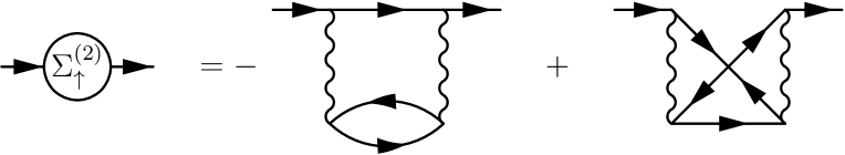
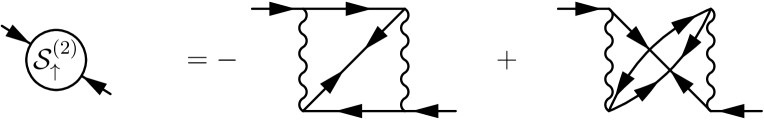
Figure 1: Diagrammatic representation of the two spin-up components of the second-order correction to the $d$-electron self-energy, Eq. (27). Top line represents spin-up, bottom line spin-down. Arrows with single heads (diagonal elements of the bath Green function) mark the propagation of electrons (right arrow) and holes (left arrow), arrows with double heads (off-diagonal elements of the bath Green function) represent creation and annihilation of the Cooper pairs. Vertical wavy line is the Coulomb interaction vertex $U$.

The IPT was later generalized for arbitrary filling [44] by introducing interpolation parameters $\mathcal{A}$ and $\mathcal{B}$,

$$\Sigma_{\mathrm{imp}}(i\omega_{n})=\Sigma^{\mathrm{HF}}+\mathcal{A}\Sigma^{(2)}(i\omega_{n})\left[1-\mathcal{B}\Sigma^{(2)}(i\omega_{n})\right]^{-1}.$$ (30)

Parameter $\mathcal{A}$ is obtained from the exact asymptotics in the high-frequency limit ($\omega_{n}\rightarrow\pm\infty$) of the spectral function that can be calculated from the equation of motion [45, 46] and $\mathcal{B}$ is derived from the atomic limit $t\rightarrow 0$. The matrix form of the parameters for superconducting models in the Nambu formalism was derived in Ref. [42] where the authors showed that matrix $\mathcal{B}$ is zero in the superconducting case.

Our experience with 2PT calculations of SCIAM [47, 48] shows that a more viable way how to modify the behavior of the self-energy is the correction of the static (Hartree-Fock) part $\Sigma^{\mathrm{HF}}$, so that the initial occupation matrix calculated from the bath Green function matches the final one calculated from the 2PT propagator. In this method, the dynamical self-energy (27) is calculated only once from the bath Green function $\mathcal{G}$, but the static part $\Sigma^{\mathrm{HF}}$ is consistently recalculated from Eq. (26) in which the bath propagator $\mathcal{G}$ is replaced by the 2PT propagator

$$G^{(2)}_{d,\mathrm{loc}}(i\omega_{n})=[\mathcal{G}^{-1}(i\omega_{n})-\Sigma^{\mathrm{HF}}-\Sigma^{(2)}(i\omega_{n})]^{-1}.$$ (31)

In theory, a fully self-consistent update is possible, where the $\Sigma^{(2)}$ is also calculated iteratively from $G^{(2)}_{d,\mathrm{loc}}$. Our experience, however, is that this method is numerically much more demanding and can lead to spurious behavior if used inside of a DMFT loop.

We implemented the IPT method in the Matsubara frequency formalism. While it is possible to implement the IPT solver directly in real frequencies, the complicated sub-gap structure of the impurity Green function makes such calculations problematic as one has to carefully identify the positions of the in-gap states while the local spectral functions $A_{d}(\omega)=-\mathop{\rm Im}\nolimits G_{d,\mathrm{loc}}(\omega+i0)/\pi$ and $A_{c}(\omega)=-\mathop{\rm Im}\nolimits G_{c,\mathrm{loc}}(\omega+i0)/\pi$ can be obtained reliably from the Matsubara Green function using the Padé analytic continuation technique [49].

Properties of 2PT solution for SCIAM were studied in Refs. [47, 48], showing that 2PT with corrected static self-energy as described above provides reliable results compared to NRG and QMC for weak and intermediate coupling $U$ if the ground state of the impurity model is a singlet, but it fails for the doublet ground state. As the ground state for the non-interacting ($U=0$) model is always a singlet, there is no way to switch on adiabatically the interaction and end up in the doublet state as it is separated from the singlet state by a quantum critical point. Also, it is not possible to perform a diagrammatic expansion around a doublet (or any multiplet) ground state without prior lifting of the degeneracy, e.g., by magnetic field. Therefore 2PT gives a non-physical solution for SCIAM in the doublet phase with the in-gap states pinned at the Fermi energy. This is indeed a serious limitation and one has to keep an eye on the sign of the induced gap $\nu_{d}$. Negative values of this parameter mark the situations where IPT becomes unreliable due to the above-mentioned failure of the underlying 2PT impurity solver, even though the results can show reasonable agreement with the numerically exact QMC data.

IV Results

Calculations were performed using our own DMFT code based on the TRIQS 2.2 libraries [50] and the TRIQS/CTHYB hybridization-expansion solver [51] at temperature $k_{B}T=0.025t$ with a cutoff in Matsubara frequencies $\omega_{n}^{\mathrm{max}}\geq 300t$. Few data sets were recalculated at lower temperature to assess its effect on the position of the phase boundaries. We restrict our results to the half-filled situation $n_{c}+n_{d}=2$. The DMFT cycle was started from zero self-energy and a high value of the gap parameter $\Delta$ which was recalculated in each DMFT iteration together with the chemical potential $\mu$ that fixes the total filling. The CT-HYB solver was used to obtain numerically exact results on the impurity density matrix, from which the occupancy, double occupancy and the induced pairing was calculated. These results were recalculated using IPT, showing good agreement, at least for the square lattice. The spectral function $A(\omega)$ was then obtained from the IPT Green function using the Padé analytic continuation method. An imaginary frequency offset $\eta=5.10^{-3}$ was used to guarantee the correct analytic behavior of the spectral functions.

IV.1 Phase diagrams

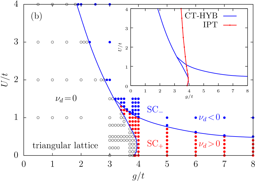
Figure 2: Phase diagram of SCPAM in the $g-U$ plane for $V=0.5t$ and $k_{B}T=0.025t$ on (a) square lattice and (b) triangular lattice calculated using CT-HYB as the DMFT solver. Bullets represent individual DMFT calculations. Black: Non-superconducting, Kondo insulator phase. Red (blue): Superconducting phase with positive (negative) induced pairing. Blue lines are approximate position of the phase boundaries. Inset: Comparison of the position of the phase boundary calculated using CT-HYB (blue) and IPT (red).

In Fig. 2 we plot the phase diagram of SCPAM in the $g-U$ plane on a square, Fig. 2(a), and triangular, Fig. 2(b), lattice at half-filling for $V=0.5t$. We choose this value of the hybridization $V$ as the superconducting correlations are strongest here in the non-interacting ($U=0$) case (see Appendix C for mode details). The two phase diagrams look rather similar, largely due to the local nature of the DMFT. The main panel shows the phase diagram calculated using CT-HYB as the DMFT solver. Each individual bullet represents a separate calculation. The black empty bullets mark the non-superconducting, KI phase. The superconducting region can be separated into two phases that we mark $\mathrm{SC_{+}}$ (red bullets) and $\mathrm{SC_{-}}$ (blue bullets) by the sign of the induced paring $\nu_{d}$. Solid lines represent the approximate position of the phase boundaries.

In the non-interacting ($U=0$) case the system is a KI for $g<g_{c0}$ and a $\mathrm{SC_{+}}$ superconductor for $g>g_{c0}$. The critical value of the attractive coupling is $g_{c0}\approx 3.30t$ for the square and $g_{c0}\approx 3.86t$ for the triangular lattice  . By increasing the interaction strength $U$, the critical coupling $g_{c}$ shows a reentrant behavior as described later in Fig. 4. The transition between the KI and $\mathrm{SC_{+}}$ phases at constant $U$ is continuous and BCS-like, i.e., $\Delta\approx(g-g_{c})^{1/2}$. The character of the transition changes at the point where the KI-superconductor transition line meets the transition line that separates the $\mathrm{SC_{+}}$ and $\mathrm{SC_{-}}$ phases. The transition from KI to $\mathrm{SC_{-}}$ phase is discontinuous with a jump in the order parameter $\Delta$. The $\mathrm{SC_{+}}$ and $\mathrm{SC_{-}}$ phases are separated by a smooth crossover that becomes sharper with decreasing temperature and the line in the phase diagram that separates these phases marks the point where the induced gap $\nu_{d}$ changes sign. The behavior of this crossover with decreasing temperature and a possible method how to extrapolate the transition to zero temperatures is discussed in Sec. IV.3.

All the presented DMFT calculations use zero self-energy and a large value of $\Delta$ as the initial condition. In the search for the expected hysteresis behavior as described by Luitz and Assaad in Ref. [25] we performed a second calculation for selected values of the coupling strength $g$, starting from the self-energy for large interaction strength $U>4t$. We encountered no measurable difference within the QMC error bars between the results at $k_{B}T=0.025t$. This is consistent with the conclusions of Ref. [25] where the authors had to perform the calculation at very low temperatures $k_{B}T\approx 0.007t$ to be able to observe any measurable hysteresis.

The insets show the phase boundaries calculated using IPT solver (red) compared to the CT-HYB result from the main panels (blue). For the square lattice IPT overestimates the value of the critical interaction strength $U$ but provides qualitatively correct topology of the phase diagram. For the triangular lattice IPT again gives a fair guess for the position of the KI-superconductor phase boundary, but fails to predict the change of the sign of the induced gap which is positive for all parameters and only decreases towards zero with increasing interaction strength $U$. This unsatisfactory behavior of the IPT for triangular lattice is connected with the failure of the solver to provide reasonable data away from half filling. As the triangular lattice is not bipartite, the fixed total filling $n_{c}+n_{d}=2$ does not guarantee that the individual bands are half-filled and the filling of the $d$ band $n_{d}$ changes with the model parameters due to the change of the chemical potential $\mu$. The IPT overestimates the deviation from half-filling of the $d$-band. Therefore the correlation effects caused by increasing $U$, which are strongest at half-filling, are damped, keeping the the system in the $\mathrm{SC_{+}}$ phase for all values of $U$.

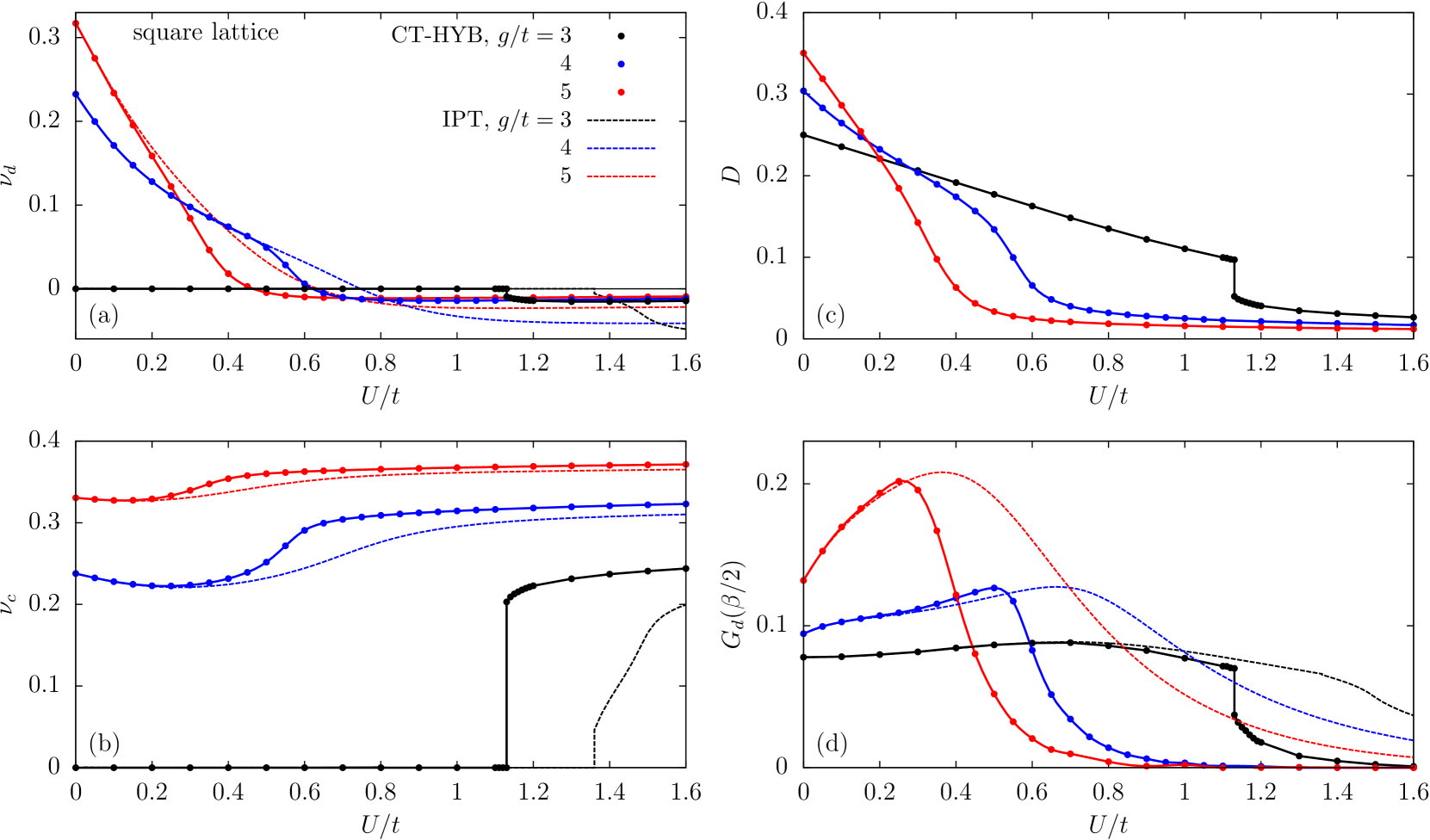
Figure 3: Induced pairing $\nu_{d}$ (a), intrinsic pairing $\nu_{c}$ (b), $d$-band double occupancy $D$ (c) and the value of the diagonal element of the imaginary-time Green function $G_{d,loc}(\tau)$ at $\tau=\beta/2$ (d) as functions of interaction strength $U$ for three values of the coupling $g$ calculated using CT-HYB (bullets) and IPT (dashed lines) as the DMFT solvers for SCPAM on the square lattice for $V=0.5t$ and $k_{B}T=0.025t$. Solid lines are splines of the quantum Monte Carlo data and serve only as a guide for the eye.

In Fig. 3 we plot the comparison of CT-HYB and IPT results along three cuts of the phase diagram for the square lattice, Fig. 2(a), for $g=3t$ (black), $4t$ (blue) and $5t$ (red). The bullets represent CT-HYB results, dashed lines IPT results. Figs. 3(a) and 3(b) show the behavior of the induced pairing $\nu_{d}$ and the intrinsic pairing $\nu_{c}$ . For $g=3t$ we start at $U=0$ from the KI phase with zero pairing. The transition to the $\mathrm{SC_{-}}$ phase is discontinuous with a jump in the order parameter at $U_{c}\approx 1.13t$. IPT overestimates this value by roughly $20\%$. The different height of the jump is also due to the proximity to the ’triple point’ where the two transition lines meet. For $g=4t$ and $5t$ the induced pairing decreases with increasing interaction strength, changing sign from positive to negative. The intrinsic $\nu_{c}$ shows a slight kink around that point, but otherwise it is largely independent of the interaction strength. IPT again overestimates the position of the transition point but provides a reasonable fit to the CT-HYB data in both superconducting phases, despite the fact it becomes unreliable in situations where $\nu_{d}$ is negative.

Fig. 3(c) shows the double occupancy of the $d$-band $D=\langle d^{\dagger}_{\uparrow}d^{\phantom{{\dagger}}}_{\uparrow}d^{\dagger}_{\downarrow}d^{\phantom{{\dagger}}}_{\downarrow}\rangle$ calculated using CT-HYB. Its value at $U=0$ is 1/4 for $g=3t$ and larger than 1/4 in the superconducting phase due to the attractive interaction induced in the impurity band by the proximity effect. It decreases with the increasing interaction strength $U$ as the doubly occupied state becomes energetically more expensive and shows a sharp downturn at the crossover to the $\mathrm{SC_{-}}$ phase, where the ground state of the impurity model is a doublet of singly-occupied states.

Fig. 3(d) shows value of the $d$-electron imaginary-time Green function $G_{d}(\tau)$ at $\tau=\beta/2$, Eq. (24), which is a measure of the spectral weight in the narrow window of a few $k_{B}T$ around the Fermi energy. For $g=3t$ the system is a KI with a narrow gap smaller than the relevant energy window so this value is small but non-zero, decreasing sharply at the transition point to the superconductor where the additional gap of width $\Delta$ opens at the Fermi energy, pushing the spectral weight to higher energies. As expected, IPT fits this value very well in the KI phase. For $g=4t$ and $5t$ this function shows a peak before the transition point, then decreases rapidly, suggesting that the subgap Andreev bands are approaching the Fermi energy at the crossover in a similar manner as the ABS are crossing in the SCIAM at the $0-\pi$ (singlet-doublet) transition. This feature is discussed in more detail in the next section.

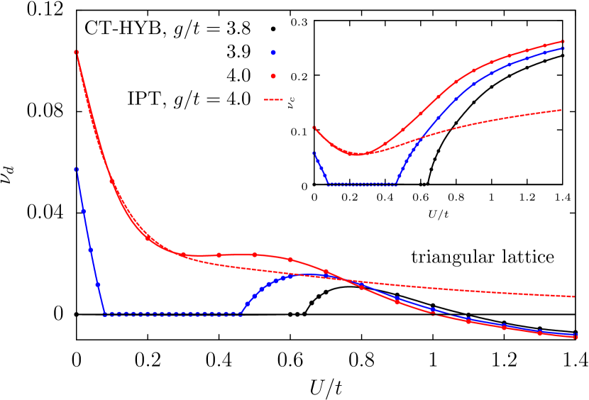
Figure 4: Induced gap $\nu_{d}$ (main panel) and the intrinsic pairing $\nu_{c}$ (inset) as functions of the interaction strength $U$ calculated using CT-HYB as the DMFT solver on the triangular lattice for three values of the electron-phonon coupling $g$ in the vicinity of the Kondo insulator - superconductor phase boundary. The system shows a reentrant behavior for $g=3.9t$ (blue). Bullets represent quantum Monte Carlo data, solid lines are splines and serve only as a guide for the eye. The dashed line represents the IPT results.

To illustrate the reentrant behavior of the superconductivity and the failure of IPT for the triangular lattice we plotted in Fig. 4 the induced pairing $\nu_{d}$ (main panel) and the intrinsic pairing $\nu_{c}$ (inset) as functions of the interaction strength $U$ for triangular lattice calculated using CT-HYB (bullets) for three values of $g$ close to the KI-$\mathrm{SC_{+}}$ phase boundary and added the IPT result for $g=4t$ (dashed line). For $g=3.9t$ the superconducting order is quickly suppressed by the increasing Coulomb interaction just to re-emerge again at higher values of $U$. Similar reentrant features are discussed in Ref. [26]. The $d$-band occupation is $n_{d}\approx 1.15$ at $U=0$ for all three values of $g$ and according to the CT-HYB result it quickly approaches unity (half filling) with increasing interaction strength. This enhances the correlation effects and eventually drives the system into the $\mathrm{SC_{-}}$ phase. On the other hand, IPT result shows only very slow decrease of the $d$ band occupation. As a result, it fails to predict the change of the sign of $\nu_{d}$ which only asymptotically approaches zero with increasing interaction strength. A more elaborate modification of the IPT algorithm is needed to correctly describe the change of the occupation to study the model on non-bipartite lattices, although this cannot overcome the principal problem of the method which is the inability to describe the spinful ground state of the impurity problem as discussed in Sec. III.2 which seriously limits the reliability of this method for certain superconducting models.

IV.2 IPT spectral functions

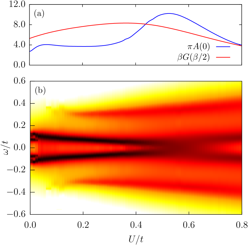
Figure 5: (a) Value of the diagonal element of the total spectral function $A(\omega)$ at the Fermi energy $\omega=0$ (blue) as a function of the interaction strength $U$ calculated using IPT for $V=0.5t$, $g=5t$, and $k_{B}T=0.025t$ compared to the $\beta G(\beta/2)$ from Fig. 3(d) (red). (b) Heatmap of $A(\omega)$ for the same parameters as in panel (a).

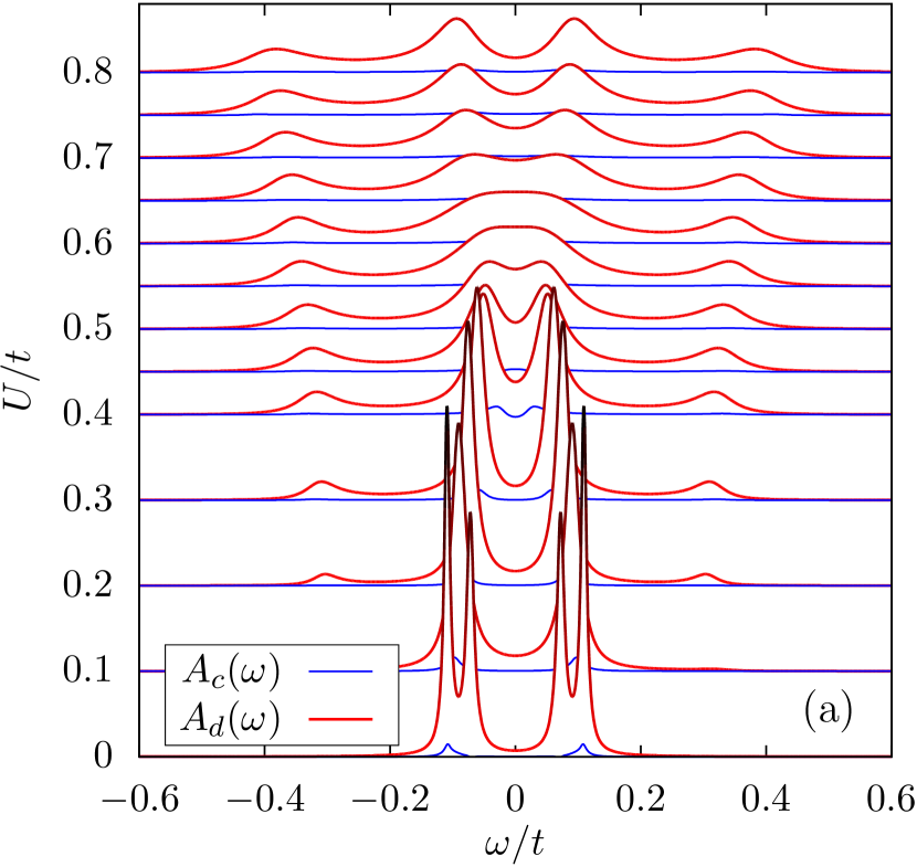
Figure 6: In-gap spectral functions $A_{c}(\omega)$ (blue) and $A_{d}(\omega)$ (red) calculated using the IPT solver for selected values of interaction strength $U$ for the same parameters as in Fig. 5, $V=0.5t$, $g=5t$, and $k_{B}T=0.025t$.

The transition between the two superconducting phases can be further illustrated on the behavior of the in-gap bands in the spectral function. Here we limit our results to the square lattice where IPT provides reasonable agreement with CT-HYB. In Fig. 5 we plot the diagonal part of the total spectral function $A(\omega)=A_{d}(\omega)+A_{c}(\omega)$ calculated using IPT as a function of the interaction strength $U$ for $V=0.5t$, $g=5t$, and $k_{B}T=0.025t$ at the Fermi energy $\omega=0$ (a) together with the heatmap of $A(\omega)$ in the region around the Fermi energy (b). We also plot in Fig. 6 the spectral function for selected values of $U$ to better specify the shape of the in-gap bands. The gap edges lie at $\pm\Delta=\pm g\nu_{c}\sim\pm 1.7t$ which follow the red dashed line from Fig. 3b (scaled by $g=5t$). As expected, the in-gap spectral function is largely dominated by the $d$-band contribution. The double-peak structure of the individual bands is quickly smeared out by the interaction strength and the two bands move closer together, losing coherence, merging at $U\approx 0.55t$ and move apart again. The merging of the bands roughly coincides with the zero of the induced pairing $\nu_{d}$ (red dashed line in Fig. 3(a)) at $U\approx 0.64t$. Furthermore, two additional bands are formed at higher energies that resemble Hubbard bands of the SIAM as they move to larger energies with increasing $U$.

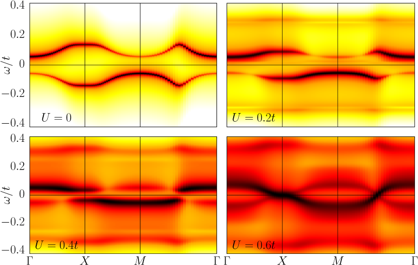
Figure 7: Momentum-resolved spectral function $A(\mathbf{k},\omega)$ for the square lattice calculated using IPT for $V=0.5t$, $g=5t$ and $k_{B}T=0.025t$ for four values of the interaction strength $U=0$ (top left), $0.2t$ (top right), $0.4t$ (bottom left), and $0.6t$ (bottom right). The notation on the high symmetry points in the Brillouin zone follows Fig. 10(c).

To further illustrate the evolution of the bands while approaching the transition point, we plot in Fig. 7 the total momentum-resolved spectral function $A(\mathbf{k},\omega)=A_{d}(\mathbf{k},\omega)+A_{c}(\mathbf{k},\omega)$ calculated using Eq. (21) in the gap region along a path in the Brillouin zone described in Fig. 10(c) for four values of the interaction strength. The double-peak structure of the bands for vanishing values of $U$ is connected with the plateaus at $\Gamma$ and $X$ points. The increasing interaction strength pushes the bands closer to the Fermi energy that can be seen on the increase of the value of $\beta G(\beta/2)$ (red line in Fig. 5(a)) that shows a maximum at $U\approx 0.4t$. As the bands are moving closer together, they simultaneously lose coherence and more spectral weight is pushed to the side bands by the increasing effect of the self-energy $\Sigma_{d}$. As $\beta G(\beta/2)$ measures the integrated spectral weight in an interval around the Fermi energy, its maximum does not match the maximum of the spectral function at the Fermi energy $A(0)$ (blue line in Fig. 5(a)), although they should become more similar with decreasing temperature and eventually coincide at $T=0$.

Fig. 7 also illustrates how the increasing self-energy is responsible for the formation of the side bands. Their evolution is similar to the formation of the Hubbard bands of the SIAM, although their position deviates for weak interaction strength from the $\omega=\pm U/2$ guess that comes from the atomic limit of the impurity model. It is more plausible these bands are, in fact, connected with the second pair of ABS that emerge in the SCIAM with doublet ground state and their origin is similar to the origin of the outer peaks in the spectrum of a single-level impurity that is simultaneously connected to both superconducting and metallic baths [55].

IV.3 Average CT-HYB expansion order

The average expansion order $\langle k\rangle$ of a CT-HYB simulation of SCPAM bears the information about the coupling between the conduction and the impurity band [35] as it can be identified with the hybridization energy scaled by inverse temperature, $\langle k\rangle=\beta\langle\mathcal{H}_{\mathrm{hyb}}\rangle$ where $\mathcal{H}_{\mathrm{hyb}}$ is given by Eq. (5). Therefore, for momentum-independent hybridization $V$ it can be related to the parameter $n_{dc}=\frac{1}{N}\sum_{\mathbf{k}}\langle d_{\mathbf{k}\sigma}^{\dagger}c_{\mathbf{k}\sigma}^{\phantom{{\dagger}}}\rangle$ defined in Eq. (22), $\langle k\rangle=2\beta Vn_{dc}$ (in contrast to the DMFT solution for the Hubbard model where $\langle k\rangle$ is connected with the kinetic energy of electrons [56]). The statistics of $k$ can be accumulated during the CT-HYB simulation and can be used to quickly identify the approximate position of the phase boundaries without the need to measure the Green function or the expectation value of any operator [57].

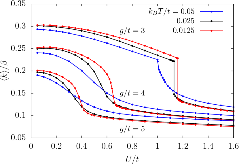
Figure 8: Average expansion order $\langle k\rangle$ of the CT-HYB simulation scaled by inverse temperature $\beta=1/k_{B}T$ as function of the interaction strength $U$ for the square lattice, $V=0.5t$, three values of the coupling strength $g$ and three temperatures $k_{B}T=0.05t$ (blue), $0.025t$ (black) and $0.0125t$ (red).

In Fig. 8 we plotted the scaled average expansion order $\langle k\rangle/\beta$ of the CT-HYB simulation as a function of the interaction strength $U$ for three values of the coupling strength $g$ and three temperatures $k_{B}T=0.05t$ (blue), $0.025t$ (black) and $0.0125t$ (red). We can use these data to assess the effect of the temperature on the position of the phase boundaries. For $g=3t$ this quantity exhibits a jump at the transition point between the KI and $\mathrm{SC_{-}}$ phases. The transition moves to higher values of $U$ and the jump becomes larger with decreasing temperature. For $g=4t$ and $5t$ the average expansion order exhibits an increasingly abrupt change with decreasing temperature around the crossover between the $\mathrm{SC_{+}}$ and $\mathrm{SC_{-}}$ phases and this crossover again moves to larger values of $U$.

For the SCIAM, the crossing of the lines for different low-enough temperatures $k_{B}T\ll\Delta$ marks the position of the phase transition at zero temperature. This can be proven by mapping the SCIAM in the vicinity of a critical point to a simple discrete two-level system [58]. In our case, the low-energy spectrum of SCPAM is continuous and the mapping is only approximate therefore the lines for different temperatures will not cross exactly at the same point, however the crossing of the lines for $k_{B}T=0.025$ (black) and $0.0125$ (red) should still give a reasonable guess for the position of the transition at zero temperatures. A comparison to the NRG data would be needed to assess the reliability of this guess for lattice models.

V Conclusions

We studied the properties of a heterostructure consisting of a periodic lattice of impurities deposited on the surface of a BCS superconductor that can be described by SCPAM. We solved the model within the DMFT framework at half filling using CT-HYB and IPT as impurity solvers. CT-HYB provides numerically exact results that showed that apart from the KI phase there are two superconducting phases we marked $\mathrm{SC_{+}}$ and $\mathrm{SC_{-}}$ separated by a crossover at finite temperatures. These phases represent analogies of the $0$ and $\pi$ phases of the SCIAM and were previously identified in Ref. [25] in a model with fixed $\Delta$ but never studied in detail. The relation between the phase transitions in the impurity model and in the lattice model bound together by the DMFT equations is still an open question [59] and here we provide an example of such scenario. We present phase diagrams at constant temperature that show the evolution of the phase boundaries with regard to the attractive interaction $g$ in the conduction band and the repulsive interaction $U$ in the impurity band. At small values of $U$ the interplay between the two interaction strengths leads to a reentrant behavior of the phase boundary between the KI and the $\mathrm{SC_{+}}$ superconductor. For larger values, the Coulomb interaction favors the $\mathrm{SC_{-}}$ superconducting phase over the KI by lowering the critical value of the attractive interaction strength. A similar effect was described in an experimental setup in which the presence of a spin-1/2 transition metal phtalocyanine molecules on the surface of a two-dimensional superconductor enhances the superconducting pairing [27]. As the CT-HYB calculation is performed in imaginary time, there is no direct way to access the spectral functions except performing an ill-defined analytic continuation. Therefore we used the approximate IPT method that provides reliable results for the square lattice. It correctly describes the KI and $\mathrm{SC_{+}}$ phases as well as crossover between the $\mathrm{SC_{+}}$ and $\mathrm{SC_{-}}$ phases. The in-gap bands follow a crossing-like scenario in which the spectral weight is transferred to the Fermi energy in the crossover region. Furthermore, a second pair of in-gap peaks is formed at higher energies. Unfortunately, the current implementation of IPT fails to describe these effects for the triangular lattice. Its reliability in the $\mathrm{SC_{-}}$ phase is also questionable due to the inherent failure of the underlying 2PT solver to correctly describe a spinful ground state of the auxiliary impurity model. In the last part we discussed the temperature dependence of the average expansion order of the CT-HYB algorithm. This quantity can be calculated very effectively and bears the information about the change of the phase boundaries with regard to the temperature.

Appendix A LDOS for square and triangular lattices

The momentum summation in Eq. (18) can be calculated effectively using the Hilbert transform and the non-interacting LDOS for the given lattice which can be calculated from the local Green function. For the square lattice with dispersion given by Eq. (11) it reads [60]

$$G_{\mathrm{loc}\square}(z)=\frac{1}{(2\pi)^{2}}\int\frac{d\mathbf{k}}{z-\varepsilon_{\mathbf{k}\square}}=\frac{2}{\pi z}K\left(\frac{16t^{2}}{z^{2}}\right),$$ (32)

where the integration is over the first Brillouin zone and

$$K(m)=\int_{0}^{\pi/2}\!\!\!\!\frac{d\theta}{\sqrt{1-m\sin^{2}(\theta)}}$$ (33)

is the complete elliptic integral of the first kind. Using the identity

$$K(m)=\frac{1}{\sqrt{m}}\left[K\left(\frac{1}{m}\right)-isK\left(1-\frac{1}{m}\right)\right],$$ (34)

where $s=\mathop{\rm sgn}\nolimits(\mathop{\rm Im}\nolimits m)$ we obtain the LDOS $A_{\square}(\omega)=-\mathop{\rm Im}\nolimits G_{\mathrm{loc}\square}(\omega+i0)/\pi$ that reads

$$A_{\square}(\omega)=\frac{1}{2\pi^{2}t}K\left(1-\frac{\omega^{2}}{16t^{2}}\right)\Theta(16t^{2}-\omega^{2}).$$ (35)

For the triangular lattice with dispersion given by Eq. (12) we obtain [60]

$$G_{\mathrm{loc}\triangle}(z)=\frac{1}{\pi\sqrt{z_{0}}}K\left(\frac{4r}{z_{0}}\right),$$ (36)

where $r=\sqrt{3-z/t}$ and $z_{0}=(r+3)(r-1)^{3}/4$. The analytic continuation to the real axis must be done carefully due to the complicated structure of the argument. The LDOS reads

$$A_{\triangle}(\omega)=\begin{cases}\frac{1}{4\pi\sqrt{z_{1}}}K\left(\frac{z_{2}}{z_{1}}\right)&\mbox{~{}for~{}}-6t<\omega<2t,\\ \frac{1}{4\pi\sqrt{z_{2}}}K\left(\frac{z_{1}}{z_{2}}\right)&\mbox{~{}for~{}}2t<\omega<3t,\\ 0&\mbox{otherwise},\end{cases}$$ (37)

where $z_{1}=4q$, $z_{2}=(3-q)(1+q)^{3}/4$, and $q=\sqrt{3-\omega/t}$. The LDOS for the square and triangular lattices are plotted in Fig. 9.

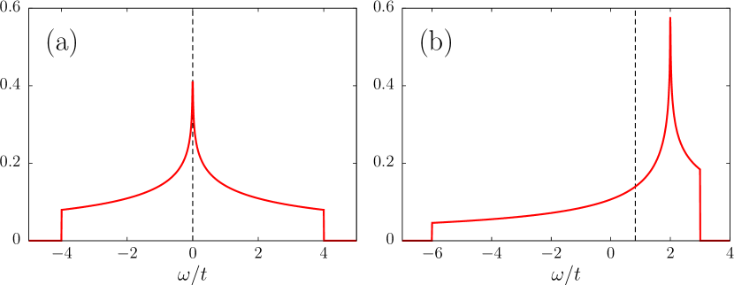
Figure 9: The non-interacting LDOS for (a) square lattice, Eq. (35) and (b) triangular lattice, Eq. (37). Dashed lines mark the position of the chemical potential that corresponds to half filling.

Appendix B Non-interacting band structure

The $U=0$ band structure of the SCPAM can be calculated from the Green function in Eq. (13). The determinant $D(\mathbf{k},\omega)=\mathrm{Det}[G^{-1}_{0}(\mathbf{k},\omega)]$ reads

$$D(\mathbf{k},\omega) =(\omega^{2}-\varepsilon^{2})(\omega^{2}-\zeta_{\mathbf{k}}^{2})$$ (38)

$$-2|V|^{2}(\omega^{2}+\varepsilon\varepsilon_{\mathbf{k}})+|V|^{4},$$

where $\zeta^{2}_{\mathbf{k}}=\Delta^{2}+\varepsilon^{2}_{\mathbf{k}}$. Its zeros $\omega(\mathbf{k})$ mark the positions of the poles of the Green function and read

$$\omega(\mathbf{k})= \pm\frac{1}{\sqrt{2}}\Bigg{[}2|V|^{2}+\zeta^{2}_{\mathbf{k}}+\varepsilon^{2}$$ (39)

$$\pm\sqrt{(\zeta_{\mathbf{k}}^{2}-\varepsilon^{2})^{2}+4|V|^{2}(\zeta^{2}_{\mathbf{k}}+\varepsilon^{2}+\varepsilon\varepsilon_{\mathbf{k}})}\Bigg{]}^{1/2}.$$

For $V=0$ the band structure simplifies to $\omega(\mathbf{k})=\{\pm\varepsilon,\pm\zeta_{\mathbf{k}}\}$. In Fig. 10 we plot the bands for $U=0$ for square, Fig. 10(a), and triangular, Fig. 10(b), lattice along the selected path through the Brillouin zone (black dashed line in Fig. 10(c)). For $\Delta=0$ (dashed blue lines) the model shows a very narrow hybridization gap at the Fermi energy. For $\Delta>0$ an additional gap opens between the conduction and the impurity bands.

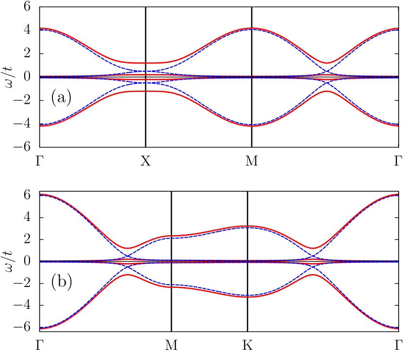
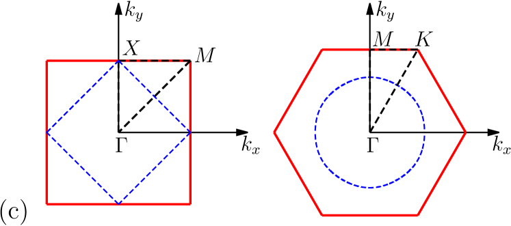
Figure 10: Non-interacting ($U=0$) band structure of the SCPAM for (a) square and (b) triangular lattice for $V=0.5t$ and $\Delta=0$ (blue dashed line), and $\Delta=t$ (red solid line). (c) First Brillouin zones for square (left) and triangular (right) lattice. Blue dashed line is the Fermi surface for $\Delta=V=0$. Black dashed line marks the path along which the data in (a) and (b) and in Fig 7 are plotted.

Appendix C Effect of hybridization and temperature on the non-interacting model

All results in Sec. IV (except Fig. 8) were calculated for the fixed value of the hybridization $V=0.5t$ and temperature $k_{B}T=0.025t$. Here we briefly discuss the effect of these parameters on the non-interacting ($U=0$) model. In Fig. 11(a) we plot the dependence of the induced pairing $\nu_{d}$ (solid lines) and intrinsic pairing $\nu_{c}$ (dashed lines) as functions of $V$ for several temperatures and $g=5t$. The increasing hybridization weakens the superconducting correlations in the conduction band measured by $\nu_{c}$ by strengthening the pair breaking effect of the magnetic impurities. The effect of the hybridization on the induced pairing $\nu_{d}$ is more complicated, as for small values of $V$ it promotes the proximity effect leading to the increase of the pairing in the impurity band, while for larger values the induced pairing decreases at the same rate as the intrinsic pairing in the conduction band. The maximum of $\nu_{d}$ for $k_{B}T=0.025t$ lies at $V\approx 0.48t$, close to the value for which the results in the main text are plotted.

In Fig. 11(b) we plot the induced pairing $\nu_{d}$ (main panel) and the intrinsic pairing $\nu_{c}$ (inset) for $g=5t$ and $U=0$ as functions of the temperature. For $T=0$ the values of $\nu_{d}$ and $\nu_{c}$ coincide for any $V>0$. For vanishing values of $V$ the intrinsic pairing decreases with increasing temperature according to the standard BCS theory and vanishes at the critical value $T_{c}$, followed by the induced pairing. For larger values of $V$ the dependence is non-monotonic and for $V=t$ (blue line) we observe the reentrant behavior of the superconductivity. This effect is also discussed in Ref. [26] and our result is in agreement with their conclusions that the reentrant behavior is not an effect of the electron correlations, as we observe it already at $U=0$, but rather a result of the subtle interplay between the electron tunneling and superconducting pairing.

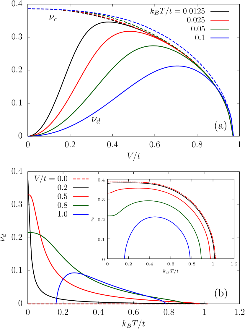
Figure 11: (a) Induced pairing $\nu_{d}$ (solid lines) and intrinsic pairing $\nu_{c}$ (dashed lines) as functions of the hybridization $V$ for selected temperatures at $U=0$ and $g=5t$. (b) Induced pairing $\nu_{d}$ (main panel) and intrinsic pairing $\nu_{c}$ (inset) as functions of the temperature for selected values of the hybridization at $U=0$ and $g=5t$.

References

- Hewson [1993] A. C. Hewson, The Kondo Problem to Heavy Fermions, Cambridge Studies in Magnetism (Cambridge University Press, 1993).
- Zhao et al. [2005] A. Zhao, Q. Li, L. Chen, H. Xiang, W. Wang, S. Pan, B. Wang, X. Xiao, J. Yang, J. G. Hou, and Q. Zhu, Controlling the Kondo effect of an adsorbed magnetic ion through its chemical bonding, Science 309, 1542 (2005).
- Balatsky et al. [2006] A. V. Balatsky, I. Vekhter, and J.-X. Zhu, Impurity-induced states in conventional and unconventional superconductors, Rev. Mod. Phys. 78, 373 (2006).
- Vojta [2006] M. Vojta, Impurity quantum phase transitions, Philos. Mag. 86, 1807 (2006).
- Luitz et al. [2012] D. J. Luitz, F. F. Assaad, T. Novotný, C. Karrasch, and V. Meden, Understanding the Josephson current through a Kondo-correlated quantum dot, Phys. Rev. Lett. 108, 227001 (2012).
- Cleuziou et al. [2006] J. P. Cleuziou, W. Wernsdorfer, V. Bouchiat, T. Ondarcuhu, and M. Monthioux, Carbon nanotube superconducting quantum interference device, Nat. Nanotechnol. 1, 53 (2006).
- Jørgensen et al. [2007] H. I. Jørgensen, T. Novotný, K. Grove-Rasmussen, K. Flensberg, and P. E. Lindelof, Critical current transition in designed Josephson quantum dot junctions, Nano Lett. 7, 2441 (2007).
- De Franceschi et al. [2010] S. De Franceschi, L. Kouwenhoven, C. Schönenberger, and W. Wernsdorfer, Hybrid superconductor-quantum dot devices, Nat. Nanotechnol. 5, 703 (2010).
- Franke et al. [2011] K. J. Franke, G. Schulze, and J. I. Pascual, Competition of superconducting phenomena and Kondo screening at the nanoscale, Science 332, 940 (2011).
- Odobesko et al. [2020] A. Odobesko, D. Di Sante, A. Kowalski, S. Wilfert, F. Friedrich, R. Thomale, G. Sangiovanni, and M. Bode, Observation of tunable single-atom Yu-Shiba-Rusinov states, Phys. Rev. B 102, 174504 (2020).
- Menth et al. [1969] A. Menth, E. Buehler, and T. H. Geballe, Magnetic and semiconducting properties of Sm, Phys. Rev. Lett. 22, 295 (1969).
- Iga et al. [1988] F. Iga, M. Kasaya, and T. Kasuya, Specific heat measurements of Yb and , J. Magn. Magn. Mater. 76-77, 156 (1988).
- Logan et al. [2016] D. E. Logan, M. R. Galpin, and J. Mannouch, Mott transitions in the periodic Anderson model, J. Phys. Condens. Matter 28, 455601 (2016).
- Vekić et al. [1995] M. Vekić, J. W. Cannon, D. J. Scalapino, R. T. Scalettar, and R. L. Sugar, Competition between antiferromagnetic order and spin-liquid behavior in the two-dimensional periodic Anderson model at half filling, Phys. Rev. Lett. 74, 2367 (1995).
- Faye et al. [2018] J. P. L. Faye, M. N. Kiselev, P. Ram, B. Kumar, and D. Sénéchal, Phase diagram of the Hubbard-Kondo lattice model from the variational cluster approximation, Phys. Rev. B 97, 235151 (2018).
- Bodensiek et al. [2013] O. Bodensiek, R. Žitko, M. Vojta, M. Jarrell, and T. Pruschke, Unconventional superconductivity from local spin fluctuations in the Kondo lattice, Phys. Rev. Lett. 110, 146406 (2013).
- Wu and Tremblay [2015] W. Wu and A.-M. S. Tremblay, -wave superconductivity in the frustrated two-dimensional periodic Anderson model, Phys. Rev. X 5, 011019 (2015).
- Ram and Kumar [2017] P. Ram and B. Kumar, Theory of quantum oscillations of magnetization in Kondo insulators, Phys. Rev. B 96, 075115 (2017).
- Ram and Kumar [2019] P. Ram and B. Kumar, Inversion and magnetic quantum oscillations in the symmetric periodic Anderson model, Phys. Rev. B 99, 235130 (2019).
- Anderson et al. [1995] M. H. Anderson, J. R. Ensher, M. R. Matthews, C. E. Wieman, and E. A. Cornell, Observation of Bose-Einstein condensation in a dilute atomic vapor, Science 269, 198 (1995).
- Koga and Werner [2010] A. Koga and P. Werner, Superfluid state in the periodic Anderson model with attractive interactions, J. Phys. Soc. Japan 79, 114401 (2010).
- Koga and Werner [2011] A. Koga and P. Werner, Superfluid state in the periodic Anderson model with attractive interactions, J. Phys. Conf. Ser. 302, 012040 (2011).
- Araújo et al. [2001] M. A. N. Araújo, N. M. R. Peres, and P. D. Sacramento, Local-moment formation in the periodic Anderson model with superconducting correlations, Phys. Rev. B 65, 012503 (2001).
- Georges et al. [1996] A. Georges, G. Kotliar, W. Krauth, and M. J. Rozenberg, Dynamical mean-field theory of strongly correlated fermion systems and the limit of infinite dimensions, Rev. Mod. Phys. 68, 13 (1996).
- Luitz and Assaad [2010] D. J. Luitz and F. F. Assaad, Weak-coupling continuous-time quantum Monte Carlo study of the single impurity and periodic Anderson models with s-wave superconducting baths, Phys. Rev. B 81, 024509 (2010).
- van Gerven Oei and Tanasković [2020] W. V. van Gerven Oei and D. Tanasković, Reentrant s-wave superconductivity in the periodic Anderson model with attractive conduction band Hubbard interaction, J. Phys. Condens. Matter 32, 325601 (2020).
- Yoshizawa et al. [2017] S. Yoshizawa, E. Minamitani, S. Vijayaraghavan, P. Mishra, Y. Takagi, T. Yokoyama, H. Oba, J. Nitta, K. Sakamoto, S. Watanabe, T. Nakayama, and T. Uchihashi, Controlled modification of superconductivity in epitaxial atomic layer–organic molecule heterostructures, Nano Letters 17, 2287 (2017).
- Uchihashi et al. [2019] T. Uchihashi, S. Yoshizawa, E. Minamitani, S. Watanabe, Y. Takagi, and T. Yokoyama, Persistent superconductivity in atomic layer-magnetic molecule van der Waals heterostructures: a comparative study, Mol. Syst. Des. Eng. 4, 511 (2019).
- Lado and Fernández-Rossier [2016] J. L. Lado and J. Fernández-Rossier, Unconventional Yu–Shiba–Rusinov states in hydrogenated graphene, 2D Mater. 3, 025001 (2016).
- Zhang et al. [2017] G. Zhang, T. Samuely, Z. Xu, J. K. Jochum, A. Volodin, S. Zhou, P. W. May, O. Onufriienko, J. Kačmarčík, J. A. Steele, J. Li, J. Vanacken, J. Vacík, P. Szabó, H. Yuan, M. B. J. Roeffaers, D. Cerbu, P. Samuely, J. Hofkens, and V. V. Moshchalkov, Superconducting ferromagnetic nanodiamond, ACS Nano 11, 5358 (2017).
- Zhang et al. [2020] G. Zhang, T. Samuely, N. Iwahara, J. Kačmarčík, C. Wang, P. W. May, J. K. Jochum, O. Onufriienko, P. Szabó, S. Zhou, P. Samuely, V. V. Moshchalkov, L. F. Chibotaru, and H.-G. Rubahn, Yu-Shiba-Rusinov bands in ferromagnetic superconducting diamond, Sci. Adv. 6, eaaz2536 (2020).
- Müller-Hartmann [1989] E. Müller-Hartmann, The Hubbard model at high dimensions: some exact results and weak coupling theory, Z. Physik B Condens. Matter 76, 211 (1989).
- Metzner and Vollhardt [1989] W. Metzner and D. Vollhardt, Correlated lattice fermions in dimensions, Phys. Rev. Lett. 62, 324 (1989).
- Kotliar et al. [2006] G. Kotliar, S. Y. Savrasov, K. Haule, V. S. Oudovenko, O. Parcollet, and C. A. Marianetti, Electronic structure calculations with dynamical mean-field theory, Rev. Mod. Phys. 78, 865 (2006).
- Gull et al. [2011] E. Gull, A. J. Millis, A. I. Lichtenstein, A. N. Rubtsov, M. Troyer, and P. Werner, Continuous-time Monte Carlo methods for quantum impurity models, Rev. Mod. Phys. 83, 349 (2011).
- Jarrell and Gubernatis [1996] M. Jarrell and J. Gubernatis, Bayesian inference and the analytic continuation of imaginary-time quantum Monte Carlo data, Phys. Rep. 269, 133 (1996).
- Liebsch [2003] A. Liebsch, Mott transitions in multiorbital systems, Phys. Rev. Lett. 91, 226401 (2003).
- Georges and Kotliar [1992] A. Georges and G. Kotliar, Hubbard model in infinite dimensions, Phys. Rev. B 45, 6479 (1992).
- Schweitzer and Czycholl [1991] H. Schweitzer and G. Czycholl, Resistivity and thermopower of heavy-fermion systems, Phys. Rev. Lett. 67, 3724 (1991).
- Rozenberg et al. [1996] M. J. Rozenberg, G. Kotliar, and H. Kajueter, Transfer of spectral weight in spectroscopies of correlated electron systems, Phys. Rev. B 54, 8452 (1996).
- Vidhyadhiraja et al. [2000] N. S. Vidhyadhiraja, A. N. Tahvildar-Zadeh, M. Jarrell, and H. R. Krishnamurthy, “Exhaustion” physics in the periodic Anderson model from iterated perturbation theory, EPL 49, 459 (2000).
- Garg et al. [2005] A. Garg, H. R. Krishnamurthy, and M. Randeria, BCS-BEC crossover at : A dynamical mean-field theory approach, Phys. Rev. B 72, 024517 (2005).
- Koley [2017] S. Koley, Pressure driven phase transition in 1T-Ti, a MOIPT+DMFT study, Solid State Commun. 251, 23 (2017).
- Kajueter and Kotliar [1996] H. Kajueter and G. Kotliar, New iterative perturbation scheme for lattice models with arbitrary filling, Phys. Rev. Lett. 77, 131 (1996).
- Geipel and Nolting [1988] G. Geipel and W. Nolting, Ferromagnetism in the strongly correlated Hubbard model, Phys. Rev. B 38, 2608 (1988).
- Nolting and Borgiel [1989] W. Nolting and W. Borgiel, Band magnetism in the Hubbard model, Phys. Rev. B 39, 6962 (1989).
- Žonda et al. [2015] M. Žonda, V. Pokorný, V. Janiš, and T. Novotný, Perturbation theory of a superconducting impurity quantum phase transition, Sci. Rep. 5, 8821 (2015).
- Žonda et al. [2016] M. Žonda, V. Pokorný, V. Janiš, and T. Novotný, Perturbation theory for an Anderson quantum dot asymmetrically attached to two superconducting leads, Phys. Rev. B 93, 024523 (2016).
- Vidberg and Serene [1977] H. J. Vidberg and J. W. Serene, Solving the Eliashberg equations by means of N-point Padé approximants, J. Low Temp. Phys. 29, 179 (1977).
- Parcollet et al. [2015] O. Parcollet, M. Ferrero, T. Ayral, H. Hafermann, I. Krivenko, L. Messio, and P. Seth, TRIQS: A toolbox for research on interacting quantum systems, Comput. Phys. Commun. 196, 398 (2015).
- Seth et al. [2016] P. Seth, I. Krivenko, M. Ferrero, and O. Parcollet, TRIQS/CTHYB: A continuous-time quantum Monte Carlo hybridisation expansion solver for quantum impurity problems, Comput. Phys. Commun. 200, 274 (2016).
- Note [1] It is worth noting that our method cannot identify a possible superconducting state that forms without explicit attractive pairing, i.e., at as discussed by Bodensiek et al. in Ref. [16]. Our order parameter is recalculated in each DMFT iteration from the intrinsic pairing and therefore it is always proportional to . As a result, we cannot rule out the existence of another SC phase where the pairing would be mediated by magnetic excitations as hypothesized in the abovementioned paper.
- Note [2] The existence of the critical value of at is connected with the fact that at half-filling the normal () state is an insulator. For fillings where the normal state is metallic at the system is a superconductor for any , assuming the temperature is smaller than the critical temperature.
- Note [3] We plot the pairing instead of the gap because the data for pairing are more commensurate for different values of and fit better in a single plot.
- Zalom et al. [2021] P. Zalom, V. Pokorný, and T. Novotný, Spectral and transport properties of a half-filled Anderson impurity coupled to phase-biased superconducting and metallic leads, Phys. Rev. B 103, 035419 (2021).
- Haule [2007] K. Haule, Quantum Monte Carlo impurity solver for cluster dynamical mean-field theory and electronic structure calculations with adjustable cluster base, Phys. Rev. B 75, 155113 (2007).
- Pokorný and Novotný [2021] V. Pokorný and T. Novotný, Footprints of impurity quantum phase transitions in quantum Monte Carlo statistics, Phys. Rev. Research 3, 023013 (2021).
- Kadlecová et al. [2019] A. Kadlecová, M. Žonda, V. Pokorný, and T. Novotný, Practical guide to quantum phase transitions in quantum-dot-based tunable Josephson junctions, Phys. Rev. Applied 11, 044094 (2019).
- Bulla [2006] R. Bulla, Dynamical mean-field theory: from quantum impurity physics to lattice problems, Philos. Mag. 86, 1877 (2006).
- Kogan and Gumbs [2021] E. Kogan and G. Gumbs, Green’s functions and DOS for some 2D lattices, Graphene 10, 1 (2021).