Bayesian inference of Lévy walks via hidden Markov models

Abstract

Abstract. The Lévy walk is a non-Brownian random walk model that has been found to describe anomalous dynamic phenomena in diverse fields ranging from biology over quantum physics to ecology. Recurrently occurring problems are to examine whether observed data are successfully quantified by a model classified as Lévy walks or not and extract the best model parameters in accordance with the data. Motivated by such needs, we propose a hidden Markov model for Lévy walks and computationally realize and test the corresponding Bayesian inference method. We introduce a Markovian decomposition scheme to approximate a renewal process governed by a power-law waiting time distribution. Using this, we construct the likelihood function of Lévy walks based on a hidden Markov model and the forward algorithm. With the Lévy walk trajectories simulated at various conditions, we perform the Bayesian inference for parameter estimation and model classification. We show that the power-law exponent of the flight-time distribution can be successfully extracted even at the condition that the mean-squared displacement does not display the expected scaling exponent due to the noise or insufficient trajectory length. It is also demonstrated that the Bayesian method performs remarkably inferring the Lévy walk trajectories from given unclassified trajectory data set if the noise level is moderate.

1 Introduction

Complex diffusion dynamics is often observed in diverse fields, such as transport dynamics of living macromolecules inside a biological cell [1, 2, 3, 4, 5, 6, 7, 8], tracer particles in polymer networks [9, 10, 11], foraging dynamics of living organisms [12, 13, 14] or animals [15, 16], and stock prices in the stock market [17, 18], to name a few. Such complex dynamics usually deviate from Brownian dynamics [19, 20, 21] characterized by Gaussian displacements $P(\Delta x;\Delta t)\propto\exp\left(-\frac{\Delta x^{2}}{4D\Delta t}\right)$ and the linear growth of the mean-squared displacement (MSD) with time $\langle x^{2}(t)\rangle\propto t$. They exhibit non-Brownian characteristics in which the MSD usually increases with time as

$$\langle x^{2}(t)\rangle\propto t^{\alpha}$$ (1)

with the anomaly exponent $\alpha$ in the range $0<\alpha\leq 2$ [22, 23] and/or the displacements have a non-Gaussian distribution that violates the central limit theorem [9, 23]. These anomalous diffusion dynamics have been explained by continuous-time random walk [24, 25], fractional Brownian motion [26], Lévy walk [27], annealed transient time [28], and scaled Brownian motion [29, 30].

It is often challenging to pinpoint the anomalous diffusion model underlying observed complex diffusion dynamics and determine the value of model parameters (e.g., the anomaly exponent). The former is understood as model classification and the latter as parameter estimation. To get proper information on these tasks, conventionally, one analyzes the experimental time-series data with various dynamic measures such as MSD, Van-Hove correlation functions, step-length or flight-time distribution, and ergodicity breaking parameter [31, 32, 33, 34, 35, 36, 37]. However, the interpretation of the data can be subjective and sometimes becomes highly nontrivial if the given data are not ideal. The non-ideal conditions include insufficient samples in terms of length and number, the high noise level in the data, and the spatiotemporal heterogeneity in the samples. To overcome these difficulties, recently, new approaches, e.g., Bayesian inference and machine learning, have been developed with keen interest from cross-disciplinary sciences  [38, 39, 40, 41, 42, 43, 10, 44, 45, 46].

In this work, we develop a Bayesian inference method for analyzing Lévy walks. Bayesian inference provides a direct comparison between the possible statistical models and finds the most likely model parameters over a given parameter space by calculating the likelihood functions of given data. In a Bayesian framework, one does not have to define point-estimators and extract the statistical features (e.g., MSD or van-Hove correlation function). From a single raw trajectory, diffusion models and model parameters can be examined to derive the best-fit model and its model parameters. Recently, some efforts have been devoted to developing the Bayesian framework for Brownian motion, fractional Brownian motion, and diffusing diffusivity [42, 43, 10, 44, 45]. These studies have proven the success of the Bayesian inference approach in the trajectory analysis.

The Lévy walk model is a physical correction of Lévy flights [27]. The corresponding trajectory consists of independent ballistic flights with constant speed $v$ and the random flight times governed by a Lévy distribution. Lévy walks are known to model various non-equilibrium dynamic processes in biology, ecology, physics, and economics. Prominent examples include foraging dynamics of bacteria, animals, and humans [47, 48, 49, 50, 51, 52, 16, 53], active transport of macromolecules inside a living cell [54, 55, 56], blinking dynamics of quantum dots [57], light in inhomogeneous media [58], a flow motion in a rotating annulus [59], and related Hamiltonian systems [60, 61]. For modeling animal’s foraging dynamics in ecology, a Bayesian inference approach was applied to differentiate Lévy flights/walks from composite correlated random walks via calculating their likelihood functions [46]. Their method, however, was based on manually-extracted step lengths and turning angles from trajectories. Moreover, the correlation between the step length and flight time—the essential ingredient of a Lévy walk—was not taken into account in the likelihood function. Previously, we developed Bayesian inference frameworks for several anomalous diffusion models [43, 10, 44, 45]. In this work, based on these experiences, we set the Bayesian inference method for Lévy walks. Our approach is based on a Markov decomposition method that mathematically describes a Lévy walk process without the manually-extracted distribution features. Using this method, we construct the likelihood function of a Lévy walk trajectory systematically as a function of trajectory length, the power-law exponent of the flight-time distribution, and the noise strength.

The present paper is organized in the following structure. In Sec. 2 we give a brief overview of Bayesian inference theory and the Lévy walk model that are used throughout the paper. In Sec. 3, we propose a theory of the hidden Markov model for Lévy walks. This model is employed to compute the likelihood function of a one dimensional Lévy walk trajectory based on the forward algorithm (we comment on a generalization to two dimensions in the B). Secs. 4 & 5 present the computational results of our Bayesian inference method. Here, we demonstrate that random flight times governed by a power-law distribution are generated from the hidden Markov model. We also visualize the numerically calculated likelihood functions at various conditions. We then systematically investigate the performance of our Bayesian inference tool for extracting the power-law exponent of Lévy walk trajectories upon varying the trajectory length, the exponent $\alpha$, and the signal-to-noise ratio. In Sec. 5, we study the model classification using the Bayesian method differentiating among Lévy walk, fractional Brownian and scaled Brownian trajectories at various conditions. Finally, in Sec. 6 we summarize our study and discuss the generalization of our Bayesian inference theory of Lévy walks for the application to other similar anomalous dynamic processes.

2 Theoretical background

2.1 Bayesian inference method

In this subsection, we provide a short overview of Bayesian inference in connection with our Bayesian approach to Lévy walks in the following section. Here we introduce key concepts as well as define essential probability distributions to be used later. For a complete overview of Bayesian inference, see Ref. [62]. Suppose that a data set $\mathcal{D}$ is given, and we have several statistical models $\mathcal{M}_{i}$ to explain the data. For a quantitative comparison between the models, in principle, we need to estimate the conditional probability $P(\mathcal{M}_{i}|\mathcal{D})$ that the model $\mathcal{M}_{i}$ is selected to explain $\mathcal{D}$. The best-fit model is the one that maximizes the given conditional probability. According to Bayes’ theorem [63], $P(\mathcal{M}_{i}|\mathcal{D})$ is given by

$$P(\mathcal{M}_{i}|\mathcal{D})=\frac{P(\mathcal{D}|\mathcal{M}_{i})P(\mathcal{M}_{i})}{P(\mathcal{D})}$$ (2)

where $P(\mathcal{M}_{i})$ is the prior probability that the model $\mathcal{M}_{i}$ is given before our observation. $P(\mathcal{D}|\mathcal{M}_{i})\equiv Z_{i}$ is the conditional probability that the data $\mathcal{D}$ is observed when a model $\mathcal{M}_{i}$ is given, referred to as evidence of a model $\mathcal{M}_{i}$. Assuming that all the prior probabilities are the same, i.e., $P(\mathcal{M}_{i})=P(\mathcal{M}_{j})$ for all $(i,~{}j)$ pairs, then the probability that the model $\mathcal{M}_{i}$ is true among $N$ possible models is given by the ratio of the model evidence:

$$\frac{P(\mathcal{M}_{i}|\mathcal{D})}{\sum_{j=1}^{N}P(\mathcal{M}_{j}|\mathcal{D})}=\frac{P(\mathcal{D}|\mathcal{M}_{i})}{\sum_{j=1}^{N}P(\mathcal{D}|\mathcal{M}_{j})}=\frac{Z_{i}}{\sum_{j=1}^{N}Z_{j}}.$$ (3)

This is the key idea in the Bayesian approach towards model inference. The best-fit model can be found via the comparison of the model evidences.

To calculate the model evidence, we define the likelihood function $\mathcal{L}_{i}(\vec{\theta}_{i})\equiv P(\mathcal{D}|\vec{\theta}_{i},\mathcal{M}_{i})$ where $\vec{\theta}_{i}$ is the parameter set necessary to specify the model $\mathcal{M}_{i}$. The model evidence (marginal likelihood) is then evaluated by marginalizing the likelihood function $\mathcal{L}_{i}(\vec{\theta}_{i})$ over the parameter space $\Theta$ with a weight $\pi(\vec{\theta}_{i})$:

$$Z_{i}=P(\mathcal{D}|\mathcal{M}_{i})=\int_{\Theta}P(\mathcal{D}|\vec{\theta}_{i},\mathcal{M}_{i})\pi(\vec{\theta}_{i})d\vec{\theta}_{i}.$$ (4)

Here, $\pi(\vec{\theta}_{i})\equiv p(\vec{\theta}_{i}|\mathcal{M}_{i})$ is a prior probability for the parameter set $\vec{\theta}_{i}$ given based on additional information or intuition [62].

The Bayesian inference approach is effectively used to find the best parameter set for a given data set if a specific model is given or the best model is determined from the above model inference. The posterior probability distribution of the parameters is given by

$$P(\vec{\theta}_{i}|\mathcal{M}_{i},\mathcal{D})=\frac{P(\mathcal{D}|\vec{\theta}_{i},\mathcal{M}_{i})P(\vec{\theta}_{i}|\mathcal{M}_{i})}{P(\mathcal{D}|\mathcal{M}_{i})}=\frac{\mathcal{L}_{i}(\vec{\theta}_{i})\pi(\vec{\theta}_{i})}{Z_{i}},$$ (5)

and we report the medians of this distribution as the estimated values of the parameters of a given model. It is computationally nontrivial to perform the marginalization of the likelihood function [Eq. (4)] and to sample over the posterior distribution (5). For this task, here we use the method of annealed importance sampling [64]. For further information on this method, see our MATLAB code for annealed importance sampling in the AnDi challenge GitHub [65].

2.2 The discrete-time Lévy walk

In the Lévy walk model, a flight time $\tau$ of a ballistic run with speed $v$ and its step length $\Delta x$ is given by the joint probability

$$\Psi(\Delta x,\tau)=\frac{1}{2}\psi(\tau)\delta(|\Delta x|-v\tau).$$ (6)

Because of the constraint between flight time and step length, the whole dynamics are solely determined by characteristics of the flight time distribution $\psi(\tau)$. In the Lévy walk we consider the class of $\psi(\tau)$ that asymptotically behaves as a power-law function at large times

$$\psi(\tau)\propto\frac{1}{\tau^{1+\gamma}}$$ (7)

with a power-law exponent $\gamma$ (i.e., the stability index of a Lévy distribution) of $0<\gamma\leq 2$. The Lévy walk has distinct diffusion dynamics depending on $\gamma$ [27]: the diffusion becomes ballistic for $0<\gamma<1$, sub-ballistic superdiffusive for $1<\gamma<2$, and diffusive for $\gamma\geq 2$. In this work, we are interested in the sub-ballistic Lévy walk where the MSD increases with time as [27]

$$\langle x^{2}(t)\rangle\propto t^{3-\gamma}~{}\hbox{at}~{}t\to\infty.$$ (8)

Thus, in this range of $\gamma$, the index of flight-time distribution [Eq. (7)] is related to the anomaly exponent via

$$\alpha=3-\gamma~{}\hbox{with}~{}1<\alpha<2.$$ (9)

For simplicity, hereafter, we denote the flight-time distribution $\psi(t)$ in terms of $\alpha$ [via Eq. (9)] throughout the text.

While the Lévy walk is defined with $\psi(\tau)$ in the continuous time-domain of $\tau>0$, time series in the experiment, such as particle trajectories obtained from a single-particle tracking experiment, are usually given in unit of a time lag that is bound by the time resolution of a measurement. To apply our Bayesian inference approach to such data, we here introduce a discrete-time Lévy walk. Practically, the Lévy walk trajectory is often generated in this way. The anomalous diffusion simulation package (the AnDi package [66, 67]) used in this work provides the discrete-time Lévy walk.

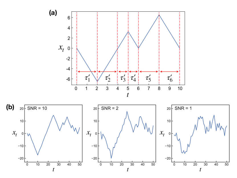
Figure 1: Sample trajectories for one-dimensional discrete-time Lévy walks. (a) A Lévy walk comprises ballistic flights whose flight events are specified by (velocity, flight time)=$\{(v_{i}=\pm v,\tau_{i})\}$. The flight times $\tau\in(0,\infty)$ are randomly given by a power-law PDF $\psi(\tau)\propto\tau^{\alpha-4}$ ($1\leq\alpha\leq 2$). In the discrete-time Lévy walk (shown in the panel), flight times are integers $\tau^{\prime}(\in\mathbb{N})$ whose probability mass function is given by Eq. (12). (b) Noisy discrete-time Lévy walk trajectories simulated from the governing equation (13) with $\alpha=1.36$. From Left to Right, the trajectories have a noise level with $\mathrm{SNR}=10,2,$ and 1. See the text for further information. The trajectories are generated by the AnDi package [66].

In the discrete-time Lévy walk, the flight times are integers, sampled by the following two steps. (1) A continuous random time $\tau(>0)$ is sampled by the transformation

$$\tau\leftarrow F^{-1}(u;\alpha)=(1-u)^{-\frac{1}{3-\alpha}}$$ (10)

using a uniform random number $u$ in $(0,1)$ and $F(t)=\int_{1}^{t}\psi(\tau)d\tau=(3-\alpha)\int_{1}^{t}\tau^{\alpha-4}d\tau$. The normalized probability density function for $\tau$ is

$$\psi_{\mathrm{c}}^{\mathrm{target}}(\tau;\alpha)=\frac{3-\alpha}{\tau^{4-\alpha}}\quad\hbox{for~{}}\tau\geq 1.$$ (11)

(2) The integer part of $\tau$ is taken using floor function $\tau^{\prime}=\lfloor\tau\rfloor$. After the rounding-off, the probability mass function for $\tau^{\prime}$ is given by

$$\psi_{\mathrm{d}}^{\mathrm{target}}(\tau^{\prime};\alpha) =\int_{\tau^{\prime}}^{\tau^{\prime}+1}\psi_{\mathrm{c}}^{\mathrm{target}}(\tau;\alpha)d\tau\quad\hbox{for}\,\,\tau^{\prime}\in\mathbb{N}$$ (12)

$$=\frac{1}{\tau^{\prime 3-\alpha}}-\frac{1}{(\tau^{\prime}+1)^{3-\alpha}}\propto\frac{1}{\tau^{\prime 4-\alpha}}.$$

From now on, we call Eq. (11) the continuous target distribution and Eq. (12) the discrete target distribution. With the integer random times given by $\psi^{\mathrm{target}}_{\mathrm{d}}(\tau^{\prime})$, we can generate a discrete-time Lévy walk trajectory parametrized by $\vec{\theta}=\left\{v,\alpha,\sigma_{\mathrm{noise}}\right\}$ via the governing equation

$$x_{t} =x_{t}^{\mathrm{LW}}+\xi_{t}$$ (13)

$$=\left[\sum_{i=1}^{N}(-1)^{r_{i}}v\tau^{\prime}_{i}+(-1)^{r_{N+1}}v\tau^{\prime}_{\mathrm{res}}\right]+\xi_{t}$$

with

$$t=\sum_{i=1}^{N}\tau^{\prime}_{i}+\tau^{\prime}_{\mathrm{res}}.$$ (14)

Figure 1(a) shows a schematic description of our discrete-time Lévy walk. For given observation time $t$, the walker (or particle) has $N$ complete flight events and an incomplete flight event. The duration time for the latter is described by a residual time $\tau^{\prime}_{\mathrm{res}}=t-\sum_{i=1}^{N}\tau^{\prime}_{i}$. The velocity of the walker during the $i$-th flight is $(-1)^{r_{i}}v$ where $r_{i}=0$ or $1$ with an equal probability. Additionally, we consider a Lévy walk in a noisy environment. Physically, the noise may originate from localization errors during the tracking measurement or the thermal random agitation in the heat bath. Thus, in a complete picture, we invent the so-called noisy Lévy walk trajectory by superimposing a Gaussian random noise $\xi_{t}$ to the noise-free trajectory in Eq. (13). The Gaussian noise is characterized by $\xi_{t}\sim\mathcal{N}(0,\sigma_{\mathrm{noise}}^{2})$ where $v/\sigma_{\mathrm{noise}}$ (or $\sigma_{D}/\sigma_{\mathrm{noise}}$ after standardizing the trajectory in the later section) is understood as the signal-to-noise (SNR) ratio. Figure 1(b) shows examples of the noisy Lévy walk trajectories for varying SNRs. When the noise level is significantly high ($\mathrm{SNR}=1$), the noisy Lévy walk no longer looks like a Lévy walk.

3 Hidden Markov model for Lévy walks & Bayesian inference

3.1 Hidden Markov model for Lévy walks

In this section, we develop our theoretical formalism of the Bayesian inference framework for Lévy walks. For this, we first build up a solvable model that appropriately describes the discrete-time Lévy walk process in the scheme of the Bayesian formalism. Our approach is to establish a hidden Markov model for non-Markovian processes governed by a power-law relaxation dynamics using the Markovian decomposition method [68].

Now let us consider a flight-time distribution with a power-law decay up to a time $T$, which is referred to as a cutoff time and usually considered the maximum observation time window in the measurement. Such power-law distributions can be represented by the superposition of a finite number of independent exponential distributions (i.e., Ornstein-Uhlenbeck processes); see the method developed in Ref. [68]. In this approximation scheme (with a slight modification), the continuous target distribution can be expanded in terms of multiple exponential distributions as such:

$$\psi_{\mathrm{c}}^{\mathrm{target}}(\tau;\alpha)\approx\sum_{i=1}^{N_{k}}P_{i;\alpha}k_{i}e^{-k_{i}(\tau-1)}\qquad(\tau\geq 1)$$ (15)

where the inverse of the relaxation time of the $i$-th component and its statistical weight are, respectively, given by

$$k_{i} =\frac{k_{\mathrm{fast}}}{b^{i}}\qquad(i=1,2,\cdots,N_{k})$$ (16)

$$P_{i;\alpha} =\frac{k_{i}^{3-\alpha}e^{-k_{i}}}{\sum_{j=1}^{N_{k}}k_{j}^{3-\alpha}e^{-k_{j}}}.$$ (17)

See the A for the validation of Eq. (15). Here, $b$ is a scale parameter, $k_{\mathrm{fast}}$ is the high-frequency cutoff, and $N_{k}$ determines the long-time exponential cutoff $T\approx(4-\alpha)b^{N_{k}}/k_{\mathrm{fast}}$. We set $b=4$, $k_{\mathrm{fast}}=8$, and $N_{k}=5$ through the work. In this scheme, we regard the power-law distributed flight times (within the observed time window) as the inter-arrival times among $N_{k}$-component independent Markov processes. The sojourn time in the state $s_{i}$ has the probability density function

$$\phi_{i}(\tau)=k_{i}e^{-k_{i}(\tau-1)}.$$ (18)

The state transition from state $s_{i}$ to state $s_{j}$ occurs with a probability $P_{j;\alpha}$ when the process leaves the state $s_{i}$. This process gives the inter-arrival time distribution Eq. (15) in the form of $\sum_{i=1}^{N_{k}}P_{i;\alpha}\phi_{i}(\tau)$.

Now we set up the proper rounding-off process to make discrete-time Markov chains of $N_{k}$ components having the inter-arrival times governed by $\psi^{\mathrm{target}}_{d}(\tau^{\prime})$. The walker’s state is renewed at every time unit such that it is changed to one of the other states (transition) or maintains the same state (self-transition). Figure 2(a) illustrates how the transition and self-transition events are determined from the continuous inter-arrival times. Let us assume that at $t=t_{0}$ the walker (Markov chain) is in the state $S_{t_{0}}=s_{i}$ and samples the transition time $\tau$ according to $\phi_{i}(\tau)$. Here $S_{t}$ denotes the walker’s state at time $t$. (i) If $1\leq\tau<2$, it is allocated to $\tau^{\prime}=1$ from the rounding-off process. Thus, the walker in the next time ($t=t_{0}+1$) should change its state to a new one, say, $S_{t_{0}+1}=s_{j}$. In this case, the state transition occurs with the transition probability

$$\left[\int_{1}^{2}\phi_{i}(\tau)d\tau\right]P_{j;\alpha}=\left(1-e^{-k_{i}}\right)P_{j;\alpha.}$$ (19)

(ii) If $\tau\geq 2$, then $\tau^{\prime}\geq 2$ and the walker stays in the same state at $t=t_{0}+1$ ($S_{t_{0}+1}=S_{t_{0}}=s_{i}$). This is the case called the self-transition, which occurs with the transition probability

$$\int_{2}^{\infty}\phi_{i}(\tau)d\tau=e^{-k_{i}}.$$ (20)

(Beware that the event of $\tau<1$ is the null case because such events are not allowed from $\phi(\tau)$). The probability that a walker in the $i$-th state has an integer sojourn time $\tau^{\prime}$ is

$$\int_{\tau^{\prime}}^{\tau^{\prime}+1}\phi_{i}(\tau)d\tau=e^{-k_{i}(\tau^{\prime}-1)}-e^{-k_{i}\tau^{\prime}},$$ (21)

which can be understood in the Markov chain description as the probability that the walker maintains the same state $(\tau^{\prime}-1)$ times and then changes its state, i.e.,

$$(e^{-k_{i}})^{\tau^{\prime}-1}\cdot(1-e^{-k_{i}})=e^{-k_{i}(\tau^{\prime}-1)}-e^{-k_{i}\tau^{\prime}}.$$ (22)

Therefore, by simply repeating the above process every time step, we obtain the process having integer inter-arrival times of $\tau^{\prime}\geq 1$ with the distribution

$$\sum_{i=1}^{N_{k}}P_{i;\alpha}\int_{\tau^{\prime}}^{\tau^{\prime}+1}\phi_{i}(\tau)d\tau =\int_{\tau^{\prime}}^{\tau^{\prime}+1}\sum_{i=1}^{N_{k}}P_{i;\alpha}\phi_{i}(\tau)d\tau\quad(\tau^{\prime}\in\mathbb{N})$$ (23)

$$\approx\int_{\tau^{\prime}}^{\tau^{\prime}+1}\psi^{\mathrm{target}}_{\mathrm{c}}(\tau;\alpha)d\tau$$

$$=\psi^{\mathrm{target}}_{\mathrm{d}}(\tau^{\prime};\alpha).$$

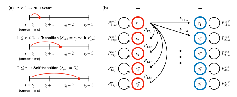
Figure 2: (a) Transition strategy of a random walker in our Markovian approximation of discrete-time Lévy walk model. A walker in a state $s_{i}^{\pm}$ samples transition time $\tau$ from $\phi_{i}(\tau)$ every time step. The probability of $\tau<1$ event (top) is zero. If a walker samples $1\leq\tau<2$ (middle), it changes the state from $s_{i}^{\pm}$ to $s_{j}^{\pm}$ with probability $P_{j;\alpha}$ ($\frac{1}{2}P_{j;\alpha}$ for each of the two states $s_{j}^{+}$ and $s_{j}^{-}$). If a walker chooses $2\leq\tau$ (bottom), it maintains its original state ($S_{t+1}=S_{t}$). (b) Schematic illustration of hidden Markov model for one-dimensional Lévy walk. In this model, the ‘$+$’ states (red circles) have positive velocity $+v$ and ‘$-$’ states (blue circles) have negative velocity $-v$. The probabilities of self-transitions and transitions for every time step are denoted by $P_{ii;\alpha}^{\mathrm{self}}$ and $P_{ij;\alpha}$, which are given by (25) and (24), respectively.

Figure 2B illustrates our Markov chain scheme based on the above formalism. Here we incorporate the fact that the Lévy walk (in 1D) has two velocity states, $\pm v$, for given flight time. This is described in our model such that the state $s_{i}$ has two substates $s_{i}^{+}$ (for $+v$) and $s_{i}^{-}$ (for $-v$) with the same transition rate $k_{i}$. Thus, there are $2N_{k}$ states in total in the model and the transition probability from the $i$-th state to the $j$-th state is given by

$$P_{ij;\alpha}=\frac{(1-e^{-k_{i}})\cdot P_{j;\alpha}}{2}.$$ (24)

As shown in Fig. 2(b), the change of the velocity state from $s_{i}^{+}$($s_{i}^{-}$) to $s_{i}^{-}$($s_{i}^{+}$) is considered as a transition with the probability $P_{ii;\alpha}$. On the other hand, if the process changes its state from $s_{i}^{+}(s_{i}^{-})$ to $s_{i}^{+}(s_{i}^{-})$, this is effectively a self-transition. The effective probability of self-transition is then given by

$$P_{ii;\alpha}^{\mathrm{self}}=e^{-k_{i}}+\frac{(1-e^{-k_{i}})\cdot P_{i;\alpha}}{2}.$$ (25)

We numerically confirm our hidden Markov model for discrete-time Lévy walks in Sec. 4.1.

3.2 The likelihood function

The above discrete-time Markov chain describes the dynamics of the latent states $S_{t}$. For given parameter set $\vec{\theta}=\{\alpha,v,\sigma_{\mathrm{noise}}\}$ and $S_{t}$, the conditional probability of observing $\Delta x_{t}=x_{t+1}-x_{t}$, i.e., the so-called emission probability, is given by

$$P(\Delta x_{t}|\mathcal{M}_{\mathrm{L\acute{e}vy}},S_{t},\vec{\theta})=\frac{1}{\sqrt{4\pi\sigma_{\mathrm{noise}}^{2}}}\exp\left(-\frac{1}{2}\left(\frac{\Delta x_{t}\pm v}{\sqrt{2}\sigma_{\mathrm{noise}}}\right)^{2}\right).$$ (26)

In this expression, $\Delta x_{t}-v$ corresponds to the state $S_{t}=s_{i}^{+}$ ($i=1,\ldots,N_{k}$) and $\Delta x_{t}+v$ to the state $S_{t}=s_{i}^{-}$, respectively. The factor $\sqrt{2}\sigma_{\mathrm{noise}}$ is attributed to the fact that the displacement is $\Delta x_{t}=x_{t+1}^{\mathrm{LW}}-x_{t}^{\mathrm{LW}}+\xi^{\prime}_{t}$ where $\xi^{\prime}_{t}$ is a Gaussian random noise of $\mathcal{N}(0,2\sigma^{2}_{\mathrm{noise}})$. We consider this term as an approximate way to include measurement noise for the positions, i.e., we should really have had $\xi^{\prime}_{t}=\xi_{t+1}-\xi_{t}$ with the $\xi_{t}$ independent. This approximation ignores the correlations between steps that measurement noise induces, and we will see later that it does not work well when $\sigma_{\mathrm{noise}}$ is comparable to the Levy walk step size, i.e., when $\mathrm{SNR}$ is not larger than unity. For brevity, below we omit the notation of $\mathcal{M}_{\mathrm{L\acute{e}vy}}$ in the conditional probabilities.

In the discrete-time Lévy walk, a trajectory $x_{t}$ can be represented by a series of the unit-time displacements $\mathcal{D}=\{\Delta x_{1},\Delta x_{2},\cdots,\Delta x_{T}\}$. Thus, when the latent state is given by $\mathcal{S}=\left\{S_{1},S_{2},\cdots,S_{T}\right\}$, the probability of finding $\mathcal{D}$ (or $x_{t}$) is written as the product of the emission probabilities

$$P(\mathcal{D}|\mathcal{S},\vec{\theta})=P(\Delta x_{1}|S_{1},\vec{\theta})P(\Delta x_{2}|S_{2},\vec{\theta})\cdots P(\Delta x_{T}|S_{T},\vec{\theta}).$$ (27)

We should marginalize Eq. (27) over all possible sequences of the latent state $\mathcal{S}=\{S_{1},S_{2},\cdots,S_{T}\}$ to obtain the likelihood function

$$P(\mathcal{D}|\vec{\theta})=\sum_{\mathcal{S}}P(\mathcal{D}|\mathcal{S},\vec{\theta})P(\mathcal{S}|\vec{\theta}).$$ (28)

In this work, we use the forward algorithm method to calculate Eq. (28) for obtaining the corresponding likelihood function [69]. The summation over $\mathcal{S}$ is carried out in an iterative way with the help of the probability function

$$\beta(S_{t}=s_{i}^{\pm})\equiv P(\Delta x_{1},\cdots,\Delta x_{t},S_{t}=s_{i}^{\pm}|\vec{\theta}).$$ (29)

This probability function satisfies the recurrence relation

$$\beta(S_{t+1}=s_{i}^{\pm}) =P(\Delta x_{1},\cdots,\Delta x_{t},\Delta x_{t+1},S_{t+1}=s_{i}^{\pm}|\vec{\theta})$$ (30)

$$=P(\Delta x_{t+1}|S_{t+1}=s_{i}^{\pm},\vec{\theta})$$

$$\quad\times\sum_{j=1}^{N_{k}}\left[\beta(S_{t}=s_{j}^{+})P(S_{t+1}=s_{i}^{\pm}|S_{t}=s_{j}^{+})\right.$$

$$\qquad\qquad+\left.\beta(S_{t}=s_{j}^{-})P(S_{t+1}=s_{i}^{\pm}|S_{t}=s_{j}^{-})\right].$$

In this expression, we figure that $P(\Delta x_{t}|S_{t}=s_{i}^{\pm},\vec{\theta})$ is the emission probability (26) and $P(S_{t+1}=s_{i}^{\pm}|S_{t}=s_{j}^{\pm})$ is the transition probabilities between two distinct states [Eq. (24)] or between the same state (self-transition) [Eq. (25)]. The initial condition of the recurrence relation is

$$\beta(S_{1}=s_{i}^{\pm}) =P(\Delta x_{1},S_{1}=s_{i}^{\pm}|\vec{\theta})$$ (31)

$$=P(\Delta x_{1}|S_{1}=s_{i}^{\pm},\vec{\theta})P(S_{1}=s_{i}^{\pm}).$$

The initial distribution of the states $P(S_{1}=s_{i}^{\pm})$ is given by Eq. (17) provided that the process starts at $t=0$ (or more generally, the initial time $t=0$ is the renewal time). Alternatively, if the process is observed after a long time where it has become stationary, then an extra factor of the average length of the time intervals, $C/(1-e^{-k_{i}})$, should be multiplied on the right hand side of Eq. (17) to obtain the initial distribution. $C$ is a normalizing constant of the distribution.

The recurrence relation Eq. (31) is given in terms of the transition probability, emission probability, and the initial distribution of the states that can be computable. Therefore, starting from Eq. (31), we can iteratively obtain $\beta(S_{T}=s_{i}^{\pm})=P(\Delta x_{1},\cdots,\Delta x_{T},S_{T}=s_{i}^{\pm}|\vec{\theta})$. The likelihood function is then simply obtained by marginalizing $\beta(S_{T}=s_{i}^{\pm})$ over all possible states:

$$P(\mathcal{D}|\vec{\theta})=P(\Delta x_{1},\cdots,\Delta x_{T}|\vec{\theta})=\sum_{i=1}^{N_{k}}\left[\beta(S_{T}=s_{i}^{+})+\beta(S_{T}=s_{i}^{-})\right].$$ (32)

Note that changes in direction and observations of the Lévy walker can only happen at integer values of time. In case observations happen with a camera that is operated independently of the system it observes, this can be considered an approximation that is valid in the limit of the camera frame rate being much faster than the typical interval between changes of direction.

3.3 Prior distributions

For Bayesian inference, we need to specify the prior distributions for parameters $\vec{\theta}=\{\alpha,v,\sigma_{\mathrm{noise}}\}$. We use a uniform prior distribution for the anomaly exponent $\alpha$ based on the fact that our Lévy walk describes a superdiffusive and Fickian dynamics with the anomaly exponent in the range of $1\leq\alpha\leq 2$. The prior distribution is set to be $P(\alpha)=1$ for $1\leq\alpha\leq 2$ or zero otherwise. For the walker’s speed $v(>0)$, we use a folded Gaussian distribution $P(v)=\sqrt{\frac{2}{\pi}}\exp\left(-\frac{v^{2}}{2}\right)$ in the positive regime. We use the Gaussian distribution because the trajectories we analyze in Sec. 4 have a standard normal distribution of speed $v$ after standardization. The pre-processing (standardization) of the trajectories is further explained in Sec. 4.2. In the case of the background noise strength $\sigma_{\mathrm{noise}}$, its magnitude compared to the signal can be arbitrary. Here, we use a folded Cauchy distribution $P(\sigma_{\mathrm{noise}})=\frac{2}{\pi\left(1+\sigma_{\mathrm{noise}}^{2}\right)}$ with $\sigma_{\mathrm{noise}}>0$ as a prior distribution. The Cauchy distribution is a heavy-tailed distribution, allowing $\sigma_{\mathrm{noise}}$ to be an arbitrarily large value.

4 Results I: Numerical implementation of the Bayesian inference and parameter estimation

4.1 Numerical implementation of the hidden Markov model

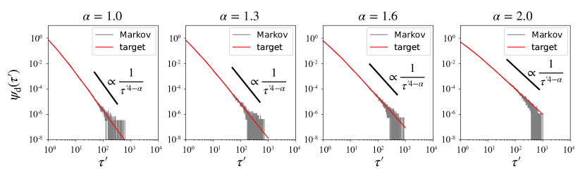
Figure 3: Flight time statistics sampled from the inter-arrival times for our Markov chain model (gray lines). In the simulation of the Markov chain model we use the parameters $N_{k}=5$, $b=4$, $k_{\mathrm{fast}}=8$, and $\alpha=1.0,\,1.3,\,1.6,$ and $2.0$ (from Left to Right). The red lines show the discrete target distribution $\psi^{\mathrm{target}}_{d}(\tau^{\prime})$ shown in Eq. (12).

We have numerically implemented our hidden Markov model for the discrete-time Lévy walk. In Fig. 3 we plot the flight-time distributions obtained from the simulated inter-arrival times of the Markov chain at $\alpha=1.0,\,1.3,\,1.6$, and $2.0$. We allocate 5000 random walkers on every Markov chain (Fig. 2(b)) and collect the inter-arrival times for the transition events between distinct latent states up to $t=1000$. For all cases, we find the numerically obtained inter-arrival times (gray lines, Fig. 3) are in excellent agreement with the expected power-law target distribution (12) (red lines). While the longest exponential cutoff is expected to start at $T\approx O(300)$, the power-law scaling in the numerical data seems to extend longer than $T$. The tail of the distribution for $t\gtrsim T$ is noisy because this part is sampled from the rare events of the $N_{k}$-th latent state. The exponential cut-off time $T$ gets shorter as $\alpha$ increases. For $\alpha=2$, the distribution shows the expected power-law up to $T\approx 256$, and then it is slightly off the power-law due to the exponential cutoff.

We numerically obtain the likelihood function by the iterative method [Eq. (32)] and confirm the validity of our method. For this purpose, we generate Lévy walk trajectories of length $100$ time steps with the flight-time exponent $\alpha=1.6$ and $v\approx 5.92$ (i) without the background noise and (ii) with the noise with $\mathrm{SNR}=2$. We estimate the likelihood function for the trajectories over the parameter space $v\in[0,10]$, $\alpha\in[1,2]$, and $\sigma_{\mathrm{noise}}\in[0.01,5]$. Figure 4 visualizes the numerically estimated likelihood functions. In the figure, the heatmaps show the likelihood functions as a function of $v$ and $\alpha$ that are marginalized over the background noise $\sigma_{\mathrm{noise}}$; the line plots are the likelihood function as a function of $\alpha$ marginalized over both $\sigma_{\mathrm{noise}}$ and $v$. All the likelihood functions are divided by their maximum value $\mathcal{L}_{\mathrm{max}}$ for normalization. (1) The noise-free Lévy walk trajectory [Fig. 4(a)]. When such ideal Lévy walk data are given, the likelihood function expectedly produces the maximum probability at the parameter ($v$, $\alpha$) that is very close to the true value. It is noted that the shape of the likelihood function around the maximum is dependent on the parameter. While the likelihood function appears to be a sharply peaked function for $v$, it is a broad distribution for $\alpha$ (see the line plot). This is because there are much more samples (displacement vectors) for inferring $v$ than for inferring $\alpha$ that relies on fewer samples of flight times. (2) The noisy Lévy walk trajectory [Fig. 4(b)]. We find that the noise makes the likelihood function dispersed in the parameter space $v$ while the profile of the likelihood function for $\alpha$ is almost unaffected by the noise. The increased uncertainty for $v$ is understandable. The speed of a flight can be fluctuating by the noise in the unit of time step. Despite the dispersion, the likelihood function still has the maximum at around the input speed. This suggests that the Bayesian approach can successfully estimate the true parameter value ($\alpha$ & $v$) even from noisy trajectories.

Figure 4: Heatmap of likelihood functions for a Lévy walk trajectory with $\alpha=1.6$ and the speed $v\approx 5.92$. (a) The likelihood function for the Lévy trajectory without the noise ($\sigma_{\mathrm{noise}}=0$). (b) The likelihood function for the trajectory with $\sigma_{\mathrm{noise}}=3$. In (a) & (b), the heatmap shows the likelihood function marginalized over $\sigma_{\mathrm{noise}}$ as a function of $v$ and $\alpha$. The line plot represents the likelihood function marginalized over $\sigma_{\mathrm{noise}}$ and $v$, where the dashed line shows the $\alpha$ at which the likelihood function gives the maximum value.

4.2 Parameter estimation via the Bayesian inference

Based on the likelihood function constructed above, we have implemented a Bayesian inference method to estimate model parameters from the trajectory data. The Lévy walk is characterized by three model parameters: the power-law exponent of flight-time distribution $\gamma=3-\alpha$ (or, equivalently, the anomaly exponent $\alpha$), the walker’s flight speed $v$, and the background noise strength $\sigma_{\mathrm{noise}}$. In this work, we focus on inferring the power-law exponent of the flight-time statistics $\alpha$ for given Lévy walk trajectories. The other parameters, such as $v$, can be easily inferred by available statistical approaches, e.g., by averaging absolute values of unit displacements.

For our study, we generate a total of 1100 Lévy walk trajectories with various trajectory lengths $N_{\mathrm{step}}\in\{10,100,200,\cdots,900,1000\}$. The trajectories are produced by the AnDi package [66]. The anomaly exponent $\alpha$ and the speed $v$ are randomly given such that $\alpha\sim\mathrm{unif}(1,2)$ and $v\sim\mathrm{unif}(0,10)$, respectively. We standardize the trajectories using the protocol described in Ref. [70], in which the trajectories are regularized so that the standard deviation of the displacement distribution has $\sigma_{D}\sim\mathcal{N}(0,1)$. This pre-processing is required to avoid the unexpected effect of step sizes on both the parameter estimation and model classification. We then add the three different levels of Gaussian noises to the 1100 trajectory with an $\mathrm{SNR}=\sigma_{D}/\sigma_{\mathrm{noise}}\in\{1,2,10\}$, thus in total generating 3300 noisy Lévy trajectories.

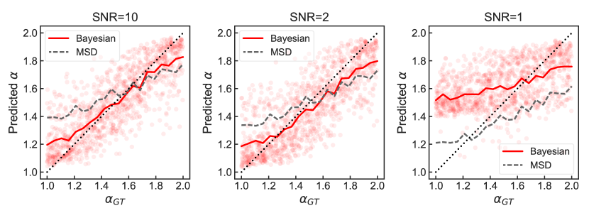
Figure 5: The predicted $\alpha$ values from our Bayesian method vs the ground-true value $\alpha_{\mathrm{GT}}$. From Left to Right, the plot correspond to $\mathrm{SNR}=10,/2,$, and 1. The solid line (red) shows the average of the predicted $\alpha$ values for given $\alpha_{\mathrm{GT}}$. For reference, the dashed line depicts the corresponding curve for $\alpha$ estimated from the fitting of time-averaged MSD curves. We fit the linear part of the MSD curves in log-log plot, where the lag time $\Delta$ ranges from $2\leq\Delta\leq 21$ for the trajectories whose lengths are over $100$. For the shorter ones, we took $2\leq\Delta\leq 8$. The dotted line is the guide line of $y=x$.

We perform our Bayesian inference analysis to these noisy Lévy walk trajectories and estimate the anomaly exponent $\alpha$, more precisely, the power-law exponent of the flight-time distribution. In Fig. 5, we compare the predicted $\alpha$ to the ground-true value $\alpha_{\mathrm{GT}}$ used for generating the data. In each scatter plot, the solid line is the average of the predicted $\alpha$ for given $\alpha_{\mathrm{GT}}$. When the background noise is not significant ($\mathrm{SNR}=10,~{}2$), the predicted $\alpha$ (solid line) is in good agreement with $\alpha_{\mathrm{GT}}$. We confirm that the estimation of $\alpha$ via the Bayesian inference is more accurate than that from the fitting of the MSD curve (the dashed line). When the noise becomes comparable with the signal ($\mathrm{SNR}=1$), both methods show poor performance.

For a more quantitative examination of the performance of our Bayesian inference method, we measure the absolute error (AE), $|\alpha_{i}-\alpha_{\mathrm{GT},i}|$, as a function of $N_{\mathrm{step}}$, $\alpha_{\mathrm{GT}}$, and SNR. In AE, $\alpha_{i}$ and $\alpha_{\mathrm{GT}}$ signify the predicted $\alpha$ and $\alpha_{\mathrm{GT}}$ for the $i$-th trajectory, respectively. In Fig. 6(a), we show the mean absolute error (MAE) as a function of $N_{\mathrm{step}}$. For $\mathrm{SNR}=10$ and $2$, the increase of trajectory length leads to more accurate estimation. For all trajectory lengths, the Bayesian method performs much better than the fitting from MSDs. For the case of $\mathrm{SNR}=1$, on the contrary, the inference goodness is not improved even if the length is increased. In this case, intense noises impede the accurate inference of flight times.

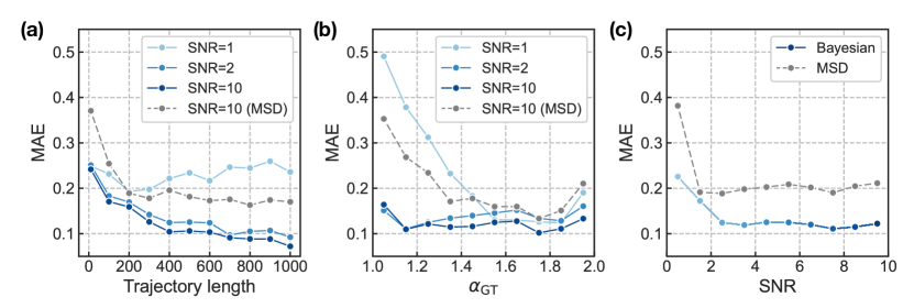
Figure 6: Mean absolute error (MAE) from our Bayesian parameter estimation (line-dot) and from the fitting of MSD curves (dashed-dot). (a) MAE as a function of the trajectory length. (b) MAE as a function of $\alpha_{\mathrm{GT}}$. Each data point represents the average value for all trajectory lengths at a given $\alpha_{\mathrm{GT}}$ with half bin width $|\Delta\alpha_{\mathrm{GT}}|=0.05$. (c) MAE as a function of SNR. Each data point represents the averaged AE for all trajectory lengths. For given $N_{\mathrm{step}}$, five hundred trajectories are generated with an SNR uniformly distributed over $(0,10]$. In $x$-axis, half bin width is $|\Delta\mathrm{SNR}|=0.5$.

Figure 6(b) shows the MAE from all trajectory lengths as a function of $\alpha_{\mathrm{GT}}$. For $\mathrm{SNR}=10$ and $2$, the inference goodness is almost insensitive to $\alpha_{\mathrm{GT}}$ although the error seems to be relatively larger at $\alpha_{\mathrm{GT}}=1$ and $2$. Note that even at $\mathrm{SNR}=10$, the MAE from the fitting method (MSD) is considerably high for these cases. When the noise level is too high ($\mathrm{SNR}=1$), the inference performance tends to be poorer as $\alpha_{\mathrm{GT}}$ is close to unity. This tendency occurs because the zigzag flight patterns frequently occurring in Lévy walk trajectories with $\alpha_{\mathrm{GT}}\sim 1$ are easily confused with the noisy dynamics (when an SNR is small), so the short flight times cannot be correctly extracted. Consequently, as seen in Fig. 5 ($\mathrm{SNR}=1$), the Lévy walk trajectory with $\alpha_{\mathrm{GT}}\approx 1$ is inferred to the Lévy walk with a predicted $\alpha>1$.

In Fig. 6(c) we examine the effect of SNR on MAE. The result shows that MAE abruptly decreases with increasing an SNR from $1$ to $\approx 2$, and after then it saturates for $\mathrm{SNR}\gtrsim 2$. This suggests that under a noisy environment the Bayesian inference method extracts the information of $\alpha$ (i.e., the power-law exponent in the flight-time distribution) with the accuracy at the noise-free condition. Surprisingly, such a robust performance is achievable against the noise level as significant as $\mathrm{SNR}\approx 2$. We also notice that even in the strong noise condition ($\mathrm{SNR}\lesssim 1$), the Bayesian inference is better than the fitting of MSD method in the parameter estimation.

5 Results II: Model classification

In this section, we apply our Bayesian inference method for classifying models and comparing their likelihoods. Our task is to compare several diffusion models for a given trajectory in the scheme of Bayesian inference and find the most probable model in accordance with the data. For this task, we additionally consider two diffusion models—apart from the Lévy walk (LW)—describing anomalous diffusion with $0<\alpha\leq 2$. The two anomalous models are fractional Brownian motion (FBM) [26] and scaled Brownian motion (SBM) [29, 30]. We refer to a recent review paper [1] for the mathematical introduction of these models and their applications to biology and various physical systems. Although the three models (LW, FBM, and SBM) can describe the superdiffusive process quantified by the MSD (1), they are based on distinct theoretical context and physical mechanisms. Accordingly, their statistical characteristics are distinguished, enabling us to use the Bayesian approach for model inference.

For a numerical test, we generate trajectory data for the three diffusion models. The data preparation is the same as in Sec. 4.2 for the noisy Lévy walk trajectory. For each model, there are a total of 1100 trajectories with $N_{\mathrm{step}}\in\{10,100,\cdots,900,1000\}$ (and 100 trajectories for given $N_{\mathrm{step}}$). The $\alpha$ is randomly sampled from $[1,2]$ for the three diffusion models. All of these trajectories are standardized and superimposed with background noise in the same way described in Sec. 4.2. The likelihood functions for FBM [44] and SBM [71] are available from our previous work. We refer to Ref. [44] for our Bayesian inference of FBM. Based on that, we have implemented the MATLAB code for the Bayesian model inference for LW, FBM, and SBM [65].

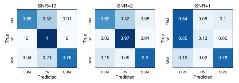
Figure 7: Confusion matrices obtained from the Bayesian model classification. From Left to Right, the matrices show the results at $\mathrm{SNR}=10$, $2$, and $1$, respectively. The $(i,j)$-component in a matrix indicates the portion of trajectories classified into the model $\mathcal{M}_{j}$ upon the true model $\mathcal{M}_{i}$.

Figure 7 shows the confusion matrices summarizing the performance of the Bayesian model classification upon the above-prepared data set. When $\mathrm{SNR}\geq 2$, our Bayesian inference gives high true positive rates for all three processes. Especially, the Lévy walk trajectory is remarkably well classified by our Bayesian method. On the contrary, if the noise level is significantly high ($\mathrm{SNR}=1$), the Lévy walk is the most poorly inferred model among the three models. In this case, the Gaussian noise tends to make the Lévy walk falsely detected as FBM (a Gaussian and stationary-incremental process). The high true positive rates for FBM and SBM at $\mathrm{SNR}=1$, comparable to those at $\mathrm{SNR}=2$ and $10$, are attributed to the same effect.

For more quantitative analysis of the model classification, we study error rates of the Lévy walk model as a function of $N_{\mathrm{step}}$, $\alpha$, and SNR. We estimate the false discovery rate (FDR) and false negative rate (FNR) from the confusion matrices. The former is the portion of FBM and SBM trajectories in the set of trajectories classified into LW, and the latter is the portion of misidentified Lévy walk trajectories (as FBM or SBM) in the set of LW trajectories.

Figure 8: Error rates obtained from confusion matrices as a function of the trajectory length, $\alpha_{\mathrm{GT}}$, and SNR. (a) & (d) False discovery rate and false negative rate of LWs as a function of the trajectory length. (b) & (e) False discovery rate and false negative rate of LWs as a function of $\alpha_{\mathrm{GT}}$ with half bin width $|\Delta\alpha_{\mathrm{GT}}|=0.05$. (c) & (f) False discovery rate and false negative rate of LWs as a function of SNR. Each data point represents the averaged value over trajectory length and $\alpha_{\mathrm{GT}}$.

Fig. 8(a) and (d), show the FDR and FNR as a function of trajectory length. The FDR tends to decrease with trajectory length irrespective of an SNR. Interestingly, FDR at $\mathrm{SNR}=1$ seems to be smaller than that for $\mathrm{SNR}\geq 2$ for most trajectory lengths. It appears that non-LW trajectories have an increased chance of being classified into our Lévy walk model when an SNR is sufficiently large. This tendency can be seen in Fig. 7 and Fig. 8(c). The FNR is shown to be very small (except for $\mathrm{SNR}=1$) and tends to decrease with the trajectory length. We note that FNR behaves against the noise in the opposite way with FDR, such that a higher noise level leads to an increased FNR. As explained, at the highest noise level ($\mathrm{SNR}=1$), the LW trajectories are apt to be classified into FBM. Here, increasing trajectory length elevates the FNR because longer trajectories contain more evidence on the noise contribution and, subsequently, increase the chance of being falsely detected as FBM.

In Fig. 8(b) & (d), we examine the variation of FDR and FNR as a function of $\alpha_{\mathrm{GT}}$. There is a clear tendency that the FDR increases as the ground true $\alpha$ approaches unity (Fig. 8(b)). This is because when $\alpha=1$ the three models converge to the same process, i.e., Brownian motion. Hence, when a given (anomalous) diffusion process has $\alpha\approx 1$, it is very difficult to pinpoint the correct underlying diffusion model. Ideally, the FDR should be $2/3$ at $\alpha_{\mathrm{GT}}=1$ if there are three models. However, FNR (at $\mathrm{SNR}=2$ and $10$) is rarely affected by the ground truth anomaly exponent. We find from further analysis of the data that ambiguous Brownian-like trajectories around $\alpha_{\mathrm{GT}}\sim 1$ tends to be classified into LW than FBM or SBM. The rise of FNR at $\mathrm{SNR}=1$ is the falsely detected FBM from the LW trajectories.

6 Discussion & Summary

In this work, we have proposed a hidden Markov model for Lévy walks (LWs) and, using this model, developed Bayesian inference tools for the analysis of LW-like trajectory data. The essential part of our theory was to approximate a renewal process governed by a power-law sojourn time distribution with a Markovian decomposition method [68]. We have shown that a power-law flight-time distribution can be generated by this method, enabling us to construct the likelihood functions of an LW. Using the Bayesian inference tool, we have demonstrated to extract the value of the power-law exponent of flight-time distribution ($\gamma=3-\alpha$) or, equivalently, the anomaly exponent $\alpha$ from given LW-like trajectories (containing background noises). It has been confirmed that the Bayesian inference method outperforms the traditional fitting method by extracting $\alpha$ from an MSD. When the noise level is negligible ($\mathrm{SNR}=10$), the accuracy of parameter estimation is as high as that by the top-performing machine learning methods recently developed [72, 70]. For the case of 2D Lévy walk trajectories, remarkably, our Bayesian inference method is shown to perform better than the top-performing machine learning tool (which will be separately reported elsewhere). Apart from the parameter estimation, we have employed our Bayesian method to classify anomalous diffusion models. For three distinct diffusion processes (LW, FBM, and SBM) superimposed with noises, our Bayesian method successfully infers the correct model with a high true positive rate when the noise level is low ($\mathrm{SNR}=10,~{}2$).

Our Bayesian inference method based on the hidden Markov model can be extended to analyzing multi-dimensional data or potentially applied to other similar problems. Below we provide some remarks on these issues.

Firstly, it is straightforward to generalize the current model for the analysis of two-dimensional (2D) Lévy walks. The 2D LWs are applicable to the modeling of cell motility on the surface [73, 74], the projected 2D motion of actively transported cargoes in the cell [75, 56], swarming dynamics of bacteria [12, 76], and various foraging dynamics in ecology [47, 48, 49, 15]. We can define a Lévy walk in 2D and construct a hidden Markov model for 2D LWs. The method is briefly sketched in the B. A full investigation of the Bayesian inference method to 2D LWs will be reported elsewhere. One remarkable result is that the estimation of $\alpha$ is more accurate in 2D than in 1D. This is attributed to the fact that successive flight events are more easily identified in 2D, which leads to the increased performance in the parameter estimation of 2D LWs at a higher SNR.

Secondly, our Lévy walk Bayesian model can be easily expanded to include composite correlated random walk (CCRW) processes via an analogous Markovian decomposite method introduced in this work. The CCRW is a multi-state random walk in which each state has a short-term (Markovian) directional memory leading to an exponential step-length distribution [46, 77]. The foraging dynamics of animals is an important example of the CCRW [16, 78, 79]. The stochastic properties of a CCRW are governed by the superposition rule of the multiple Markovian states. In the framework of CCRWs, the Lévy walk can be regarded as a special model where the superposition is specified by Eqs. (16) and (17), leading to a power-law flight-time (or step-length) distribution. The CCRW may have a different step-length distribution depending on how multiple Markovian states are superposed. By properly modeling this part, a specific CCRW can be constructed and inferred by the corresponding Bayesian method. A potential application is to identify a correct diffusion model for animal’s foraging dynamics. There is a stimulating effort in ecology for modeling the foraging motion [16, 78, 79, 80, 81, 82]. Often the analysis of the data was based on the step-length distribution (or the inverse cumulative distribution of the step lengths), which led to a debate on whether the data follows a Lévy walk having a power-law step length distribution or a different CCRW [78, 46, 16, 79]. Using the Bayesian method, one can analyze the data in a different manner and efficiently differentiate between several candidate models.

Thirdly, our hidden Markov model is applicable to construct Bayesian inference methods for variant Lévy walk models. For example, one can expand the current hidden Markov model for a Lévy walk with fluctuating velocities or a Lévy walk with a rest [27]. The latter model was shown to explain the fluid dynamics in a rotating plate and the transport of mRNA-protein complex particles in a neuron cell [54]. The Bayesian method will be helpful for extracting the information of parameters in the flight-time and rest-time distributions. Beyond the Lévy walk, once the noise correlation in the successive displacement is adequately incorporated, the current hidden Markov model can be applied to continuous-time random walks with a power-law waiting time distribution.

Finally we comment on some potential technical issues of the current Bayesian approach. The high computational cost is often required for Bayesian inference, which needs to sample parameters from high dimensional posterior distributions and calculate likelihood functions for every sampled parameter. It costs hundreds to thousands of seconds to quantify a trajectory of hundreds of steps. Notwithstanding, it is computationally feasible to handle thousands of trajectories of which step length is of $<1000$. In our study, we analyzed such trajectory data within a day using a 40-multicore workstation. Additionally, a relevant task is to improve the Bayesian inference method under a strong noise signal. In this work, we have found that the Bayesian inference analysis is vulnerable to noise when $\mathrm{SNR}\sim 1$. We anticipate that if the noise effect term in the likelihood function [Eq. (26)] was incorporated without approximation, the Bayesian inference would have a better performance to noisy trajectories under the condition of strong noise signals. We leave this task as future work.

Appendix

Appendix A Continuous-time Markov chain approximation of continuous target distribution

Here we briefly show the mathematical derivation of Eq. (15). The continuous target distribution is given by the inter-arrival time distributions and the weights as

$$\psi^{\mathrm{target}}_{\mathrm{c}}(\tau;\alpha) \approx\sum_{i=1}^{N_{k}}P_{i;\alpha}\phi_{i}(\tau)=\sum_{i=1}^{N_{k}}\left(\frac{k_{i}^{3-\alpha}e^{-k_{i}}}{\sum_{j=1}^{N_{k}}k_{j}^{3-\alpha}e^{-k_{j}}}\right)k_{i}e^{-k_{i}(\tau-1)}$$ (33)

$$=\frac{1}{\sum_{j=1}^{N_{k}}k_{j}^{3-\alpha}e^{-k_{j}}}\sum_{i=1}^{N_{k}}{k_{i}^{4-\alpha}e^{-k_{i}\tau}}.$$

In this expression, the denominator $\sum_{j=1}^{N_{k}}k_{j}^{3-\alpha}e^{-k_{j}}$ is estimated under the assumption of a sufficiently large $N_{k}$ to

$$\sum_{j=1}^{N_{k}}\left(\frac{k_{\mathrm{fast}}}{b^{j}}\right)^{3-\alpha}e^{-\frac{k_{\mathrm{fast}}}{b^{j}}} \approx\int_{\frac{1}{2}}^{\infty}dx\left(\frac{k_{\mathrm{fast}}}{b^{x}}\right)^{3-\alpha}e^{-\frac{k_{\mathrm{fast}}}{b^{x}}}$$ (34)

$$=\frac{1}{\ln b}\gamma\left(3-\alpha,k_{\mathrm{fast}}/\sqrt{b}\right)$$

where $\gamma(s,x)=\int_{0}^{x}t^{s-1}e^{-t}dt$ is the lower incomplete gamma function. The numerator can be calculated in the same way. This approximation yields

$$\sum_{i=1}^{N_{k}}P_{i;\alpha}\phi_{i}(\tau)\approx\frac{\gamma\left(4-\alpha,k_{\mathrm{fast}}\tau/\sqrt{b}\right)}{\gamma\left(3-\alpha,k_{\mathrm{fast}}/\sqrt{b}\right)}\frac{1}{\tau^{4-\alpha}}.$$ (35)

When $k_{\mathrm{fast}}$ becomes considerably large, the prefactor approaches to

$$\frac{\gamma\left(4-\alpha,k_{\mathrm{fast}}\tau/\sqrt{b}\right)}{\gamma\left(3-\alpha,k_{\mathrm{fast}}/\sqrt{b}\right)}\approx\frac{\Gamma(4-\alpha)}{\Gamma(3-\alpha)}=3-\alpha.$$ (36)

Thus, $\sum_{i=1}^{N_{k}}P_{i;\alpha}\phi_{i}(\tau)$ becomes the normalized continuous target distribution given by Eq. (11).

Appendix B Modeling two-dimensional Lévy walks

In the Markov chain approximation of 1D Lévy walk in the main text, we need two independent latent state sets ($s^{+}_{i}$ and $s^{-}_{i}$ with $i=1,2,\ldots,N_{k}$) for the flight of positive and negative directions, respectively. In the 2D Lévy walk [83], we set there are a total of $N_{\theta}$ velocity orientations (see Fig. 9(a)).

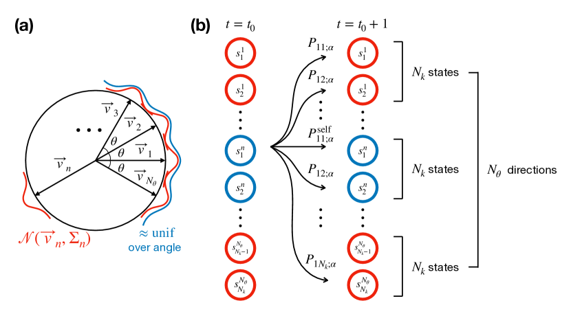
Figure 9: (a) The velocity states in our 2D Lévy walk. There are $N_{\theta}$ discrete velocity states specified by $\vec{v}_{n}$ ($n=1,2,\ldots,N_{\theta}$). We allow the orientation of $\vec{v}_{n}$ to fluctuate around the unit vector $(\cos((n-1)\theta),\sin((n-1)\theta))$, which is modeled by a Gaussian fluctuation $\mathcal{N}(\vec{v}_{n},\Sigma_{n})$. The superposition of the Gaussian fluctuations (the blue solid line) approximates the uniformly distributed velocity states over angle. (b) The Markov chain model for the 2D discrete-time Lévy walk. Each velocity states in (a) have the latent state $s^{n}_{i}$ with $i=1,2,\ldots,N_{k}$. The superscript $n$ denotes the velocity state. The transition probability from the state $s_{i}^{m}$ to $s_{j}^{n}$ is given by $P_{ij;\alpha}$ [Eq. (38)], and the self-transition probability is given by $P_{ii;\alpha}^{\mathrm{self}}$ [Eq. (37)].

A random walker can choose a random direction from the velocity vectors $\{\vec{v_{1}},\vec{v_{2}},\cdots,\vec{v_{N_{\theta}}}\}$ with a probability of $1/N_{\theta}$. We allow a velocity vector $\vec{v_{n}}$ to have uncertainty in its direction, which is modeled by a Gaussian fluctuation (see the red lines in Fig. 9(a)). We obtain a nearly uniform distribution over the velocity direction (blue line in Fig. 9(a)) once all the Gaussian fluctuations $\mathcal{N}(\vec{v}_{n},\Sigma_{n})$ are superposed.

There are a total of $N_{\theta}$ number of velocity states in the 2D Lévy walk, where there are $N_{k}$ latent states with independent transition rates $k_{i}$ $(i=1,2,\ldots,N_{k})$ for each velocity state. The probability of self-transition is

$$P_{ii;\alpha}^{\mathrm{self}}=e^{-k_{i}}+\frac{(1-e^{-k_{i}})\cdot P_{i;\alpha}}{N_{\theta}},$$ (37)

and the transition probability to other states reads

$$P_{ij;\alpha}=\frac{(1-e^{-k_{i}})\cdot P_{j;\alpha}}{N_{\theta}}.$$ (38)

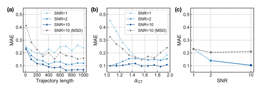
Figure 10: Parameter estimation for 2D Lévy walk trajectories. (a) Mean absolute error (MAE) as a function of the trajectory length. (b) MAE as a function of the ground-truth anomaly exponent $\alpha_{\mathrm{GT}}$. (c) MAE as a function of SNR. The dotted line is the result from the Bayesian inference and the dot-dashed line from the fitting of MSD curves.

The emission probability of an observation $\Delta\vec{x}_{t}=\vec{x}_{t+1}-\vec{x}_{t}$ from the velocity state $\vec{v}_{n}$ is given by

$$P(\Delta\vec{x}_{t}|\mathcal{M}_{\mathrm{L\acute{e}vy}},\vec{v}_{n},\Sigma_{n})=\frac{\exp\left(-\frac{1}{2}(\Delta\vec{x}_{t}-\vec{v}_{n})^{\mathrm{T}}\Sigma_{n}^{-1}(\Delta\vec{x}_{t}-\vec{v}_{n})\right)}{\sqrt{(2\pi)^{d}|\Sigma_{n}|}},$$ (39)

where $\Sigma_{n}=R(\theta_{n})\Sigma_{1}R(\theta_{n})^{\mathrm{T}}$ is a covariance matrix for Gaussian fluctuations of $\vec{v}_{n}$, $\theta_{n}$ is an angle from $x$-axis of a vector $\vec{v}_{n}$, and $R(\theta_{n})$ is a rotation matrix. From the Markov chain illustrated in Fig. 9(b) with transition probabilities (37) and (38) and the emission probability (39), the likelihood function for 2D Lévy walks can be calculated using forward algorithm as in Eqs. (27)-(32). The likelihood function for a 3D Lévy walk model can also be obtained in a similar way.

Figure 10 shows the performance of the parameter estimation. While most of the results are similar to the one-dimensional case, we notice some interesting features: The accuracy of parameter estimation has been improved at $\mathrm{SNR}=10$ compared to the corresponding case in 1D. Figure 10 shows that mean absolute error decays faster than 1D as trajectory length increases. Moreover, the MAE does not change upon the variation of anomaly exponents (Fig. 10(b)). At $\mathrm{SNR}=10$, the overall MAE decreases by $\sim 0.02$ compared to the 1D case (Fig. 10(c)).

References

- [1] Ralf Metzler, Jae-Hyung Jeon, Andrey G. Cherstvy, and Eli Barkai. Anomalous diffusion models and their properties: non-stationarity, non-ergodicity, and ageing at the centenary of single particle tracking. Phys. Chem. Chem. Phys., 16:24128–24164, 2014.
- [2] Michael J Saxton and Ken Jacobson. Single-particle tracking: applications to membrane dynamics. Annual review of biophysics and biomolecular structure, 26(1):373–399, 1997.
- [3] Ido Golding and Edward C. Cox. Physical nature of bacterial cytoplasm. Phys. Rev. Lett., 96:098102, Mar 2006.
- [4] Jae-Hyung Jeon, Vincent Tejedor, Stas Burov, Eli Barkai, Christine Selhuber-Unkel, Kirstine Berg-Sørensen, Lene Oddershede, and Ralf Metzler. In vivo anomalous diffusion and weak ergodicity breaking of lipid granules. Phys. Rev. Lett., 106:048103, Jan 2011.
- [5] Carmine Di Rienzo, Vincenzo Piazza, Enrico Gratton, Fabio Beltram, and Francesco Cardarelli. Probing short-range protein brownian motion in the cytoplasm of living cells. Nature communications, 5(1):1–8, 2014.
- [6] Diego Krapf and Ralf Metzler. Strange interfacial molecular dynamics. Physics today, 72(9):48–55, 2019.
- [7] Daniel SW Lee, Ned S Wingreen, and Clifford P Brangwynne. Chromatin mechanics dictates subdiffusion and coarsening dynamics of embedded condensates. Nature Physics, 17(4):531–538, 2021.
- [8] Seongyu Park, O-chul Lee, Xavier Durang, and Jae-Hyung Jeon. A mini-review of the diffusion dynamics of dna-binding proteins: experiments and models. Journal of the Korean Physical Society, 78(5):408–426, 2021.
- [9] Bo Wang, James Kuo, Sung Chul Bae, and Steve Granick. When brownian diffusion is not gaussian. Nature Materials, 11(6):481–485, 2012.
- [10] Andrey G. Cherstvy, Samudrajit Thapa, Caroline E. Wagner, and Ralf Metzler. Non-gaussian, non-ergodic, and non-fickian diffusion of tracers in mucin hydrogels. Soft Matter, 15:2526–2551, 2019.
- [11] Won Kyu Kim, Richard Chudoba, Sebastian Milster, Rafael Roa, Matej Kanduč, and Joachim Dzubiella. Tuning the selective permeability of polydisperse polymer networks. Soft Matter, 16(35):8144–8154, 2020.
- [12] Gil Ariel, Amit Rabani, Sivan Benisty, Jonathan D Partridge, Rasika M Harshey, and Avraham Be’Er. Swarming bacteria migrate by lévy walk. Nature communications, 6(1):1–6, 2015.
- [13] Emiliano Perez Ipiña, Stefan Otte, Rodolphe Pontier-Bres, Dorota Czerucka, and Fernando Peruani. Bacteria display optimal transport near surfaces. Nature Physics, 15(6):610–615, 2019.
- [14] AE Patteson, Arvind Gopinath, M Goulian, and PE Arratia. Running and tumbling with e. coli in polymeric solutions. Scientific reports, 5(1):1–11, 2015.
- [15] Nicolas E Humphries, Nuno Queiroz, Jennifer RM Dyer, Nicolas G Pade, Michael K Musyl, Kurt M Schaefer, Daniel W Fuller, Juerg M Brunnschweiler, Thomas K Doyle, Jonathan DR Houghton, et al. Environmental context explains lévy and brownian movement patterns of marine predators. Nature, 465(7301):1066–1069, 2010.
- [16] Monique de Jager, Franz J. Weissing, Peter M. J. Herman, Bart A. Nolet, and Johan van de Koppel. Lévy walks evolve through interaction between movement and environmental complexity. Science, 332(6037):1551–1553, 2011.
- [17] Gregor Wergen, Miro Bogner, and Joachim Krug. Record statistics for biased random walks, with an application to financial data. Phys. Rev. E, 83:051109, May 2011.
- [18] Vasiliki Plerou, Parameswaran Gopikrishnan, Luís A. Nunes Amaral, Xavier Gabaix, and H. Eugene Stanley. Economic fluctuations and anomalous diffusion. Phys. Rev. E, 62:R3023–R3026, Sep 2000.
- [19] Robert Brown F.R.S. Hon. M.R.S.E. & R.I. Acad. V.P.L.S. Xxvii. a brief account of microscopical observations made in the months of june, july and august 1827, on the particles contained in the pollen of plants; and on the general existence of active molecules in organic and inorganic bodies. The Philosophical Magazine, 4(21):161–173, 1828.
- [20] Albert Einstein. Investigations on the Theory of the Brownian Movement. Courier Corporation, 1956.
- [21] M. von Smoluchowski. Zur kinetischen theorie der brownschen molekularbewegung und der suspensionen. Annalen der Physik, 326(14):756–780, 1906.
- [22] Julia F. Reverey, Jae-Hyung Jeon, Han Bao, Matthias Leippe, Ralf Metzler, and Christine Selhuber-Unkel. Superdiffusion dominates intracellular particle motion in the supercrowded cytoplasm of pathogenic acanthamoeba castellanii. Scientific Reports, 5(1):11690, 2015.
- [23] Thomas J. Lampo, Stella Stylianidou, Mikael P. Backlund, Paul A. Wiggins, and Andrew J. Spakowitz. Cytoplasmic rna-protein particles exhibit non-gaussian subdiffusive behavior. Biophysical Journal, 112(3):532–542, 2017.
- [24] Harvey Scher and Elliott W. Montroll. Anomalous transit-time dispersion in amorphous solids. Phys. Rev. B, 12:2455–2477, Sep 1975.
- [25] Elliott W. Montroll. Random walks on lattices. iii. calculation of first-passage times with application to exciton trapping on photosynthetic units. Journal of Mathematical Physics, 10(4):753–765, 1969.
- [26] Benoit B Mandelbrot and John W Van Ness. Fractional brownian motions, fractional noises and applications. SIAM review, 10(4):422–437, 1968.
- [27] Vasily Zaburdaev, S Denisov, and J Klafter. Lévy walks. Reviews of Modern Physics, 87(2):483, 2015.
- [28] P. Massignan, C. Manzo, J. A. Torreno-Pina, M. F. García-Parajo, M. Lewenstein, and G. J. Lapeyre. Nonergodic subdiffusion from brownian motion in an inhomogeneous medium. Phys. Rev. Lett., 112:150603, Apr 2014.
- [29] SC Lim and SV Muniandy. Self-similar gaussian processes for modeling anomalous diffusion. Physical Review E, 66(2):021114, 2002.
- [30] Jae-Hyung Jeon, Aleksei V Chechkin, and Ralf Metzler. Scaled brownian motion: a paradoxical process with a time dependent diffusivity for the description of anomalous diffusion. Physical Chemistry Chemical Physics, 16(30):15811–15817, 2014.
- [31] Ralf Metzler, Vincent Tejedor, J-H Jeon, Y He, WH Deng, S Burov, and E Barkai. Analysis of single particle trajectories: From normal to anomalous diffusion. Acta Physica Polonica B, 40(5), 2009.
- [32] Jae-Hyung Jeon, Natascha Leijnse, Lene B Oddershede, and Ralf Metzler. Anomalous diffusion and power-law relaxation of the time averaged mean squared displacement in worm-like micellar solutions. New Journal of Physics, 15(4):045011, apr 2013.
- [33] Hadiseh Safdari, Andrey G Cherstvy, Aleksei V Chechkin, Felix Thiel, Igor M Sokolov, and Ralf Metzler. Quantifying the non-ergodicity of scaled brownian motion. Journal of Physics A: Mathematical and Theoretical, 48(37):375002, aug 2015.
- [34] Andrey G. Cherstvy and Ralf Metzler. Ergodicity breaking and particle spreading in noisy heterogeneous diffusion processes. The Journal of Chemical Physics, 142(14):144105, 2015.
- [35] Stas Burov, Jae-Hyung Jeon, Ralf Metzler, and Eli Barkai. Single particle tracking in systems showing anomalous diffusion: the role of weak ergodicity breaking. Phys. Chem. Chem. Phys., 13:1800–1812, 2011.
- [36] Dominique Ernst, Jürgen Köhler, and Matthias Weiss. Probing the type of anomalous diffusion with single-particle tracking. Phys. Chem. Chem. Phys., 16:7686–7691, 2014.
- [37] E. Kepten, A. Weron, G. Sikora, K. Burnecki, and Y. Garini. Guidelines for the fitting of anomalous diffusion mean square displacement graphs from single particle tracking experiments. PLoS One, 10(2):e0117722, 2015.
- [38] Vida Jamali, Cory Hargus, Assaf Ben-Moshe, Amirali Aghazadeh, Hyun Dong Ha, Kranthi K. Mandadapu, and A. Paul Alivisatos. Anomalous nanoparticle surface diffusion in lctem is revealed by deep learning-assisted analysis. Proceedings of the National Academy of Sciences, 118(10), 2021.
- [39] Gorka Muñoz-Gil, Miguel Angel Garcia-March, Carlo Manzo, José D Martín-Guerrero, and Maciej Lewenstein. Single trajectory characterization via machine learning. New Journal of Physics, 22(1):013010, jan 2020.
- [40] Frank Cichos, Kristian Gustavsson, Bernhard Mehlig, and Giovanni Volpe. Machine learning for active matter. Nature Machine Intelligence, 2(2):94–103, 2020.
- [41] Naor Granik, Lucien E. Weiss, Elias Nehme, Maayan Levin, Michael Chein, Eran Perlson, Yael Roichman, and Yoav Shechtman. Single-particle diffusion characterization by deep learning. Biophysical Journal, 117(2):185–192, 2019.
- [42] Martin Lysy, Natesh S. Pillai, David B. Hill, M. Gregory Forest, John W. R. Mellnik, Paula A. Vasquez, and Scott A. McKinley. Model comparison and assessment for single particle tracking in biological fluids. Journal of the American Statistical Association, 111(516):1413–1426, 2016.
- [43] Samudrajit Thapa, Michael A. Lomholt, Jens Krog, Andrey G. Cherstvy, and Ralf Metzler. Bayesian analysis of single-particle tracking data using the nested-sampling algorithm: maximum-likelihood model selection applied to stochastic-diffusivity data. Phys. Chem. Chem. Phys., 20:29018–29037, 2018.
- [44] Jens Krog, Lars H Jacobsen, Frederik W Lund, Daniel Wüstner, and Michael A Lomholt. Bayesian model selection with fractional brownian motion. Journal of Statistical Mechanics: Theory and Experiment, 2018(9):093501, sep 2018.
- [45] Jens Krog and Michael A. Lomholt. Bayesian inference with information content model check for langevin equations. Phys. Rev. E, 96:062106, Dec 2017.
- [46] Marie Auger-Méthé, Andrew E. Derocher, Michael J. Plank, Edward A. Codling, and Mark A. Lewis. Differentiating the lévy walk from a composite correlated random walk. Methods in Ecology and Evolution, 6(10):1179–1189, 2015.
- [47] David A. Raichlen, Brian M. Wood, Adam D. Gordon, Audax Z. P. Mabulla, Frank W. Marlowe, and Herman Pontzer. Evidence of lévy walk foraging patterns in human hunter–gatherers. Proceedings of the National Academy of Sciences, 111(2):728–733, 2014.
- [48] A. M. Reynolds and C. J. Rhodes. The lévy flight paradigm: random search patterns and mechanisms. Ecology, 90(4):877–887, 2009.
- [49] Ketika Garg and Christopher T. Kello. Efficient lévy walks in virtual human foraging. Scientific Reports, 11(1):5242, 2021.
- [50] Marina E. Wosniack, Marcos C. Santos, Ernesto P. Raposo, Gandhi M. Viswanathan, and Marcos G. E. da Luz. The evolutionary origins of lévy walk foraging. PLOS Computational Biology, 13(10):1–31, 10 2017.
- [51] Injong Rhee, Minsu Shin, Seongik Hong, Kyunghan Lee, Seong Joon Kim, and Song Chong. On the levy-walk nature of human mobility. IEEE/ACM Transactions on Networking, 19(3):630–643, 2011.
- [52] Stefano Focardi, Paolo Montanaro, and Elena Pecchioli. Adaptive lévy walks in foraging fallow deer. PLOS ONE, 4(8):1–6, 08 2009.
- [53] Haiyan Huo, Rui He, Rongjing Zhang, Junhua Yuan, and Gladys Alexandre. Swimming escherichia coli cells explore the environment by lévy walk. Applied and Environmental Microbiology, 87(6):e02429–20, 2021.
- [54] Minho S. Song, Hyungseok C. Moon, Jae-Hyung Jeon, and Hye Yoon Park. Neuronal messenger ribonucleoprotein transport follows an aging lévy walk. Nature Communications, 9(1):344, 2018.
- [55] Naama Gal and Daphne Weihs. Experimental evidence of strong anomalous diffusion in living cells. Phys. Rev. E, 81:020903, Feb 2010.
- [56] Kejia Chen, Bo Wang, and Steve Granick. Memoryless self-reinforcing directionality in endosomal active transport within living cells. Nature Materials, 14(6):589–593, 2015.
- [57] Fernando D. Stefani, Jacob P. Hoogenboom, and Eli Barkai. Beyond quantum jumps: Blinking nanoscale light emitters. Physics Today, 62(2):34–39, 2009.
- [58] Pierre Barthelemy, Jacopo Bertolotti, and Diederik S. Wiersma. A lévy flight for light. Nature, 453(7194):495–498, 2008.
- [59] T. H. Solomon, Eric R. Weeks, and Harry L. Swinney. Observation of anomalous diffusion and lévy flights in a two-dimensional rotating flow. Phys. Rev. Lett., 71:3975–3978, Dec 1993.
- [60] J. Klafter and G. Zumofen. Lévy statistics in a hamiltonian system. Phys. Rev. E, 49:4873–4877, Jun 1994.
- [61] T. Geisel, J. Nierwetberg, and A. Zacherl. Accelerated diffusion in josephson junctions and related chaotic systems. Phys. Rev. Lett., 54:616–619, Feb 1985.
- [62] Andrew Gelman, John B Carlin, Hal S Stern, David B Dunson, Aki Vehtari, and Donald B Rubin. Bayesian data analysis. CRC press, 2013.
- [63] Thomas Bayes. An essay towards solving a problem in the doctrine of chances. Philosophical Transactions of the Royal Society of London, 53:370–418, 1763.
- [64] Radford M. Neal. Annealed importance sampling. Statistics and Computing, 11(2):125–139, 2001.
-
[65]
Bayesian inference for andi challenge.
https://github.com/mlomholt/andi. accessed: 2021-06-03. - [66] Gorka Muñoz-Gil, Borja Requena, Giovanni Volpe, Miguel Angel Garcia-March, and Carlo Manzo. AnDiChallenge/ANDI_datasets: Challenge 2020 release, May 2021.
- [67] Gorka Muñoz-Gil, Giovanni Volpe, Miguel Angel García-March, Ralf Metzler, Maciej Lewenstein, and Carlo Manzo. The anomalous diffusion challenge: single trajectory characterisation as a competition. Emerging Topics in Artificial Intelligence 2020, Aug 2020.
- [68] Igor Goychuk. Viscoelastic subdiffusion: From anomalous to normal. Phys. Rev. E, 80:046125, Oct 2009.
- [69] L.R. Rabiner. A tutorial on hidden markov models and selected applications in speech recognition. Proceedings of the IEEE, 77(2):257–286, 1989.
- [70] Gorka Muñoz-Gil, Giovanni Volpe, Miguel Angel Garcia-March, Erez Aghion, Aykut Argun, Chang Beom Hong, Tom Bland, Stefano Bo, J. Alberto Conejero, Nicolás Firbas, Òscar Garibo i Orts, Alessia Gentili, Zihan Huang, Jae-Hyung Jeon, Hélène Kabbech, Yeongjin Kim, Patrycja Kowalek, Diego Krapf, Hanna Loch-Olszewska, Michael A. Lomholt, Jean-Baptiste Masson, Philipp G. Meyer, Seongyu Park, Borja Requena, Ihor Smal, Taegeun Song, Janusz Szwabiński, Samudrajit Thapa, Hippolyte Verdier, Giorgio Volpe, Arthur Widera, Maciej Lewenstein, Ralf Metzler, and Carlo Manzo. Objective comparison of methods to decode anomalous diffusion, 2021. arXiv:2105.06766.
- [71] Samudrajit Thapa. Bayesian inference with scaled brownian motion. Journal of Physics A: Mathematical and Theoretical, 2021.
-
[72]
Andi interactive tool.
https://andi-app.herokuapp.com/andi_app. accessed: 2021-06-03. - [73] Taeseok Daniel Yang, Jin-Sung Park, Youngwoon Choi, Wonshik Choi, Tae-Wook Ko, and Kyoung J Lee. Zigzag turning preference of freely crawling cells. PLoS One, 6(6):e20255, 2011.
- [74] Hui Li, Shuhong Qi, Honglin Jin, Zhongyang Qi, Zhihong Zhang, Ling Fu, and Qingming Luo. Zigzag generalized levy walk: the in vivo search strategy of immunocytes. Theranostics, 5(11):1275, 2015.
- [75] Sergei Fedotov, Nickolay Korabel, Thomas A. Waigh, Daniel Han, and Victoria J. Allan. Memory effects and lévy walk dynamics in intracellular transport of cargoes. Phys. Rev. E, 98:042136, Oct 2018.
- [76] Avraham Be’er and Gil Ariel. A statistical physics view of swarming bacteria. Movement ecology, 7(1):1–17, 2019.
- [77] Edward A Codling, Michael J Plank, and Simon Benhamou. Random walk models in biology. Journal of The Royal Society Interface, 5(25):813–834, 2008.
- [78] Vincent A. A. Jansen, Alla Mashanova, and Sergei Petrovskii. Comment on “lévy walks evolve through interaction between movement and environmental complexity”. Science, 335(6071):918–918, 2012.
- [79] Andy M. Reynolds. Mussels realize weierstrassian lévy walks as composite correlated random walks. Scientific Reports, 4(1):4409, 2014.
- [80] Andy M. Reynolds. Distinguishing between lévy walks and strong alternative models: reply. Ecology, 95(4):1109–1112, 2014.
- [81] Simon Benhamou. Detecting an orientation component in animal paths when the preferred direction is individual-dependent. Ecology, 87(2):518–528, 2006.
- [82] Simon Benhamou. How many animals really do the lévy walk? Ecology, 88(8):1962–1969, 2007.
- [83] V. Zaburdaev, I. Fouxon, S. Denisov, and E. Barkai. Superdiffusive dispersals impart the geometry of underlying random walks. Phys. Rev. Lett., 117:270601, Dec 2016.