Published in Journal of Magnetism and Magnetic Materials, Vol. 535, 168057, 2021 DOI: 10.1016/j.jmmm.2021.168057 MagTense: a micromagnetic framework using the analytical demagnetization tensor R. Bjørk, E. B. Poulsen, K. K. Nielsen, and A. R. Insinga We present the open source micromagnetic framework, MagTense, which utilizes a novel discretization approach of rectangular cuboid or tetrahedron geometry “tiles” to analytically calculate the demagnetization field. Each tile is assumed to be uniformly magnetized, and from this assumption only, the demagnetization field can be analytically calculated. Using this novel approach we calculate the solution to the $\mu$mag standard micromagnetic problems 2, 3 and 4 and find that the MagTense framework accurately predicts the solution to each of these. Finally, we show that simulation time can be significantly improved by performing the dense demagnetization tensor matrix multiplications using NVIDIA CUDA.

1 Introduction

At the microscopic scale, magnetic systems can be described by the formalism of micromagnetics. The purpose of this formalism is to determine the magnetization field within magnetic materials, and to calculate its time-evolution. Micromagnetic models are used for a plethora of magnetic calculations, including e.g. micromagnetics of rare-earth efficient permanent magnets Fischbacher et al. [2018]; Gong et al. [2019] and calculation of spin waves in nanometre-scale patterned magnetic elements Kim [2010]. The physics of micromagnetics can only in rare cases be solved analytically, and therefore numerical models are needed to simulate the physical behavior of the studied systems. Numerous micromagnetic models exist and some are also published as open source software Donahue and Porter [1999]; Vansteenkiste et al. [2014]; Leliaert et al. [2018].

In a micromagnetic model, the governing equations must be discretized and represented by a finite number of degrees of freedom Kumar and Adeyeye [2017], and a number of distinct interactions takes place between the discretized moments in the systems. These interactions can be described by different magnetic fields, such as an exchange field and an anisotropy field. Of these it is the calculation of the demagnetization field, also known as the stray field, that is the most time consuming part Abert et al. [2013]. There are in general three methods that have been applied to calculate the demagnetization field: finite difference based fast Fourier transform methods, tensor-grid methods and finite-element methods, although other methods such as fast multipole methods also exist Van de Wiele et al. [2008]; Palmesi et al. [2017]; Kumar and Adeyeye [2017]. All methods have inherent advantages and shortcomings. The finite difference Fourier-based approaches are extremely fast but unfortunately require that the magnetic moments lie on a regular grid Vansteenkiste and Van de Wiele [2011]; Vansteenkiste et al. [2014]; Ferrero and Manzin [2020], although methods for non-uniform grids Livshitz et al. [2009]; Exl and Schrefl [2014] and multi-layer materials Lepadatu [2019] have also been proposed. The tensor-grid method Exl et al. [2012] is still under investigation for stability and correctness Abert et al. [2013]. The finite element method allows easy meshing of complex geometries but also requires that an environment outside the object of interest is modelled to ensure that the correct field is calculated.

So far the direct analytical calculation of the demagnetization field has only been explored in combination with a Fourier transform method Vansteenkiste and Van de Wiele [2011]. Here we present a novel micromagnetic model that uses an analytically exact approach to calculate the full demagnetization tensor for computations in real space. This ensures that the calculated magnetic field is correct, and at the same time allows for easy meshing of complex geometries. The disadvantage is an increase in the computational cost of the model.

2 Physics of the model

2.1 Governing equations

In the following we will denote the magnetization field by $\boldsymbol{M}(\boldsymbol{x})$, where $\boldsymbol{x}$ denotes an arbitrary point. One of the fundamental assumptions in micromagnetism is that the norm of $\boldsymbol{M}$ is equal at all points to the saturation magnetization $M_{s}$. Therefore, it is customary to express the magnetization field as $\boldsymbol{M}(\boldsymbol{x})=M_{s}\boldsymbol{m}(\boldsymbol{x})$, where $\boldsymbol{m}$ is the reduced magnetization that is normalized at any point. For heterogeneous materials the saturation magnetization can also be space-dependent, but it is always assumed to be a local known property of the magnetic material.

The equation of motion governing the dynamics of micromagnetic systems is the Landau-Lifshitz equation J. García-Cervera [2014]:

$$\frac{d\boldsymbol{m}}{dt}=-\gamma\;{\boldsymbol{m}}\times\boldsymbol{H}_{\text{\scriptsize eff}}-\alpha\;{\boldsymbol{m}}\times\left({\boldsymbol{m}}\times\boldsymbol{H}_{\text{\scriptsize eff}}\right)$$ (1)

where $\boldsymbol{H}_{\text{\scriptsize eff}}$ denotes the effective field, a generalization of the concept of magnetic field that incorporates the effect of different interaction mechanisms. Indeed, the Landau-Lifshitz equation is a time-dependent partial differential equation within continuum physics that describes macroscopic classical effects as well as a semiclassical treatment of collective quantum effects.

The first and second terms on the right-hand side of Eq. 1 are called the precessional and damping term, respectively. In fact, at any point the reduced magnetization vector precesses around the effective field with a frequency determined by the gyromagnetic ratio $\gamma$ and rotates towards the effective field with a speed determined by the damping parameter $\alpha$. Due to the damping term, the cross product $\boldsymbol{m}\times\boldsymbol{H}_{\text{\scriptsize eff}}$ decreases over time, thus reducing the precession amplitude. At equilibrium, the magnetization vector is aligned with the effective field at any point. Therefore, the equilibrium state is described by the first Brown’s equation:

$$\boldsymbol{m}\times\boldsymbol{H}_{\text{\scriptsize eff}}=\boldsymbol{0}$$ (2)

As can be seen from Eq. 1, when this condition is verified the magnetization is stationary: $\frac{d\boldsymbol{m}}{dt}=\boldsymbol{0}$. Similarly, the second Brown’s equation states that, at the border of the magnet

$${\bf{m}}\times\left(A_{\text{\scriptsize exch}}\frac{\partial\bf{m}}{\partial\bf{n}}\right)=\bf{0},$$ (3)

where $A_{\text{\scriptsize exch}}$ is the exchange interaction constant and $\bf{n}$ is the normal vector of the boundary. Since $\bf{m}$ and $\frac{\partial\bf{m}}{\partial\bf{n}}$ are orthogonal, Eq. 3 can only be fulfilled by $\frac{\partial\bf{m}}{\partial\bf{n}}=0$, which corresponds to Neumann boundary conditions. It should also be stressed that the Landau-Lifshitz equation preserves the norm of $\boldsymbol{m}$ at any point.

2.2 Free energy and effective field

The effective field is associated with the micromagnetic free energy of the system, denoted by $\mathcal{G}$. The free energy is expressed as the volume integral of a corresponding volumetric energy density $g$:

$$\mathcal{G}[\boldsymbol{m}]=\int_{\Omega}dV\;g(\boldsymbol{x},\boldsymbol{m},\boldsymbol{\boldsymbol{\nabla}}m_{x},\boldsymbol{\boldsymbol{\nabla}}m_{y},\boldsymbol{\boldsymbol{\nabla}}m_{z})$$ (4)

where $\Omega$ denotes the region occupied by the magnetic material. As can be seen from Eq. 4, the energy density may depend on the magnetization $\boldsymbol{m}$ and the spatial gradients of its $x$, $y$ and $z$ components. The effective field is proportional to the first variation of the free energy with respect to $\boldsymbol{m}$:

$$\boldsymbol{H}_{\text{\scriptsize eff}}=-\frac{1}{\mu_{0}M_{s}}\frac{\delta\mathcal{G}}{\delta\boldsymbol{m}}$$ (5)

where $\mu_{0}$ denotes the vacuum permeability. Therefore, the damping term in the Landau-Lifshitz equation has the effect of decreasing the free energy, and the minima of $\mathcal{G}$ with respect to $\boldsymbol{m}$ are equilibrium configurations, i.e. satisfying Brown’s first equation.

2.3 Interaction mechanisms

As mentioned in Sec. 2.1, the effective field is composed of several terms associated with different interaction mechanisms, each obtained from a corresponding term of the free energy by calculating the first variation.

• External field - This term represents the classical macroscopic magnetostatic interaction of the magnetization vector with an external applied $\boldsymbol{H}_{a}$. The energy density is given by:

  $$g_{\text{\scriptsize ext}}=-\mu_{0}M_{s}(\boldsymbol{m}\cdot\boldsymbol{H}_{a})$$ (6)

  The effective field associated with this interaction is simply coincident with the applied field itself:

  $$\left(\boldsymbol{H}_{\text{\scriptsize eff}}\right)_{\text{\scriptsize ext}}=\boldsymbol{H}_{a}$$ (7)

• Demagnetization field - Similar to the interaction with the external field, the demagnetization term expresses the classical magnetostatic interaction of the magnetization with the field $\boldsymbol{H}_{d}$ generated in $\Omega$ by its own magnetization $\boldsymbol{M}(\boldsymbol{x})$:

  $$g_{\text{\scriptsize demag}}=-\left(\frac{\mu_{0}M_{s}}{2}\right)(\boldsymbol{m}\cdot\boldsymbol{H}_{d})$$ (8)

  The demagnetization field depends linearly on $\boldsymbol{m}$ according to the following expression:

  $$\boldsymbol{H}_{d}(\boldsymbol{x})=\int_{\Omega}dV^{\prime}\,\underline{\underline{N}}(\boldsymbol{x},\boldsymbol{x}^{\prime})\,\boldsymbol{m}(\boldsymbol{x}^{\prime})$$ (9)

  where $\underline{\underline{N}}$ denotes the demagnetization tensor. As for the previous term, the effective field associated with this interaction is coincident with the demagnetization field:

  $$\left(\boldsymbol{H}_{\text{\scriptsize eff}}\right)_{\text{\scriptsize demag}}=\boldsymbol{H}_{d}$$ (10)

  The effect of this interaction is to reduce the field generated outside $\Omega$ by driving the magnetization vector at any point towards the local magnetic field, thus forming closed loops.

• Exchange interaction - This term is a semiclassical treatment of a collective quantum effect. Derived from the Heisenberg Hamiltonian, it expresses the tendency of the magnetization vector in a point to align to the magnetization vector of the surrounding points. In the semiclassical formalism this is achieved by minimizing the spatial derivatives of $\boldsymbol{m}$:

  $$g_{\text{\scriptsize exch}}=A_{\text{\scriptsize exch}}\,\Big{(}\|\boldsymbol{\boldsymbol{\nabla}}m_{x}\|^{2}+\|\boldsymbol{\boldsymbol{\nabla}}m_{y}\|^{2}+\|\boldsymbol{\boldsymbol{\nabla}}m_{z}\|^{2}\Big{)}$$ (11)

  where $A_{\text{\scriptsize exch}}$ denotes the exchange interaction constant. The effective field associated with the exchange interaction can be computed from the corresponding energy density using variational methods:

  $$\left(\boldsymbol{H}_{\text{\scriptsize eff}}\right)_{\text{\scriptsize exch}}=\left(\frac{2A_{\text{\scriptsize exch}}}{\mu_{0}M_{s}}\right)\left(\frac{\partial^{2}\boldsymbol{m}}{\partial x^{2}}+\frac{\partial^{2}\boldsymbol{m}}{\partial y^{2}}+\frac{\partial^{2}\boldsymbol{m}}{\partial z^{2}}\right).$$ (12)

  The effect of this interaction is thus analogous to that of a vector diffusion equation, i.e. driven by magnetization gradients across $\Omega$. As for $M_{s}$, $A_{\text{\scriptsize exch}}$ may be space-dependent for heterogeneous materials, in which case the effective field would be

  $$\left(\boldsymbol{H}_{\text{\scriptsize eff}}\right)_{\text{\scriptsize exch}}=\left(\frac{2}{\mu_{0}M_{s}}\right)\nabla\cdot\left(A_{\text{\scriptsize exch}}\nabla\boldsymbol{m}\right)$$ (13)

  and in case of an abrupt material change,

  $$A_{\text{\scriptsize exch}_{1}}\frac{\partial\bf{m}}{\partial{\bf{n}}_{1}}=A_{\text{\scriptsize exch}_{2}}\frac{\partial\bf{m}}{\partial{\bf{n}}_{2}},$$ (14)

  where $\bf{n}$ is the normal vector to the material interface. Eq. 14 is nothing but a generalization of the second Brown’s equation, Eq. 3. For simplicity we do not consider this dependence here, but it would be a relatively straightforward extension of the Neumann boundary conditions already present on the boundary of the magnet.

• Crystal anisotropy - This term describes the anistropic effects due to the local orientation of the crystal lattice. For the case of uni-axial anisotropy, the energy density is expressed as:

  $$g_{\text{\scriptsize anis}}=-K(\boldsymbol{m}\cdot\hat{\boldsymbol{e}}_{K})^{2}$$ (15)

  where $K$ denotes the anisotropy constant and $\hat{\boldsymbol{e}}_{K}$ is a unit vector oriented along the easy axis of the crystal. These two parameters can also be space-dependent. Typically, $\hat{\boldsymbol{e}}_{K}$ has a different direction in each crystal grain. The effective field associated to the uni-axial anisotropy term is given by:

  $$\left(\boldsymbol{H}_{\text{\scriptsize eff}}\right)_{\text{\scriptsize anis}}=\frac{2K}{\mu_{0}M_{s}}(\boldsymbol{m}\cdot\hat{\boldsymbol{e}}_{K})\hat{\boldsymbol{e}}_{K}.$$ (16)

  Therefore, the effect of this term is to rotate the magnetization vector towards the local direction of the easy axis, i.e. $\pm\hat{\boldsymbol{e}}_{K}$. When the anisotropy constant is negative, this term rotates $\boldsymbol{m}$ away from $\pm\hat{\boldsymbol{e}}_{K}$, towards the plane that is normal to $\hat{\boldsymbol{e}}_{K}$. In this case, $\hat{\boldsymbol{e}}_{K}$ and its normal plane are referred to as “hard axis” and “easy plane”, respectively.

These four interactions are the most well studied mechanisms within the field of micromagnetics. However, it is possible to model other physical phenomena with a similar formalism, e.g. magnetostriction Rotarescu et al. [2019] or the Dzyaloshinskii-Moriya interaction Perez et al. [2014] (also called antisymmetric exchange interaction) or thermal fluctuations Ragusa et al. [2009].

3 Implementation: the MagTense framework

Except for a few cases, most notably that of a uniformly magnetized particle described by the Stoner-Wohlfarth model, micromagnetics problems can only be approached by means of numerical computations. It is thus necessary to discretize the governing equations so that $\boldsymbol{m}(\boldsymbol{x})$ is represented by a finite number of degrees of freedom. As mentioned previously the most common discretization methods are finite elements methods and finite difference methods typically with a Fourier-based approach. Generally, the computation of the demagnetization field introduced in Eq. 9 is the most computationally intensive task in the calculation and evolution of $\boldsymbol{m}(\boldsymbol{x})$.

In this work, we present a novel open-source micromagnetism and magnetostatic framework MagTense, which uses neither the finite difference nor the finite element approach to calculating the demagnetization field, but instead relies on an analytically correct expression of the demagnetization tensor. The discretization approach used in MagTense subdivides the region $\Omega$ into $N$ “tiles”, adjacent to each other. The magnetization field $\boldsymbol{m}(\boldsymbol{x})$ is thus represented by a vector of $3N$ components, three for each tile.

The demagnetization field generated by each of the tiles at the centers of all of the other tiles is computed analytically by assuming that the tile is uniformly magnetized. The analytical expression of the demagnetization tensor $\underline{\underline{N}}$ is known for many different shapes, such as the rectangular cuboid (rectangular prism) Smith et al. [2010] and the tetrahedron Nielsen et al. [2019], thus allowing great flexibility to build meshes that are suitable for the geometry being investigated. The total demagnetization field at any point is obtained by summing the individual contributions from all the tiles in the magnet domain $\Omega$. This concept is illustrated in Fig. 1 for a magnet domain meshed as rectangular prisms.

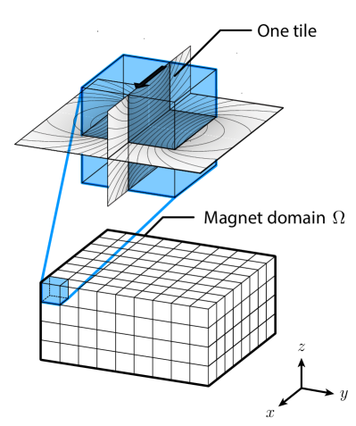
Figure 1: An illustration of the tile concept used in MagTense. The magnetic field calculated by a single prism tile along an $xz$- and $xy$-plan is also illustrated.

Besides the calculation of the demagnetization field, the other components of the effective field must also be calculated, i.e. the exchange field, the external field and anisotropy field. For the case of a Cartesian mesh of rectangular cuboids the exchange interaction field can easily be computed by applying standard finite difference schemes. However, several methods are also available for the case of unstructured polyhedral meshes Sozer et al. [2014]. These will be discussed in a subsequent work, as determining the ideal differential operator for an unstructured mesh is not a trivial task. The implementation of the external field and anisotropy terms is straightforward, as these only depend on the local properties of the tile.

3.1 The numerical implementation

In the following, we will denote with the symbol $\boldsymbol{m}$ the $3N$-element vector representing the magnetization field over the discretized mesh. Since the exchange, anisotropy and demagnetization terms of the free energy are all quadratic with respect to $\boldsymbol{m}$, the corresponding terms of the effective field are linear. Therefore, they can all be computed by multiplying the $3N$-element vector by corresponding $3N\times 3N$ matrices Insinga et al. [2020]. The exchange and anisotropy matrices are sparse matrices, whereas the demagnetization matrix is dense, which is generally the reason why computing this term is the most intensive part of a micromagnetic calculation Abert et al. [2013]. The external field energy is linear with respect to $\boldsymbol{m}$, implying that the corresponding effective field does not depend on $\boldsymbol{m}$. Denoting by $\underline{\underline{A}}$ the matrix associated with the quadratic terms, and by $\boldsymbol{b}$ the vector associated with the external field term, the $k^{\text{\scriptsize{th}}}$ component of the total effective field is computed as:

$$\left(\boldsymbol{H}_{\text{\scriptsize eff}}\right)_{k}=\sum_{j=1}^{3N}A_{kj}m_{j}+b_{k}\quad\text{for}\;k=1,\dots,3N$$ (17)

All the matrices need to be computed only once, at the beginning of the simulation. As the magnetization field evolves during the simulation according to Eq. 1, the effective field is updated and the time-derivative of each component of $\boldsymbol{m}$ can be computed. The integration of the equation of motion is here performed with an explicit Runge-Kutta (4,5) formula.

The framework MagTense is available in both a version that performs the matrix calculations on the CPU, but also a version that uses CUDA for performing the dense matrix-multiplication needed to calculate the demagnetization field, for increasing the calculation speed Lopez-Diaz et al. [2012]; Leliaert and Mulkers [2019]. All examples presented here as well as all model software is available from www.magtense.org Bjørk and Nielsen [2019]. The MagTense micromagnetic model is available both in the FORTRAN programming language and Matlab computing environment. The FORTRAN version can be directly interfaced with Matlab through a MEX-interface. A Python interface is available for the magnetostatic part of MagTense at present.

3.2 Computational resources

The challenge in using the full demagnetization tensor for micromagnetic simulations is that the demagnetization tensor scales as $N^{2}$ where $N$ is the number of tiles. This is in contract to e.g. the FFT method, where the storage requirement is only of size $N$ and the computational complexity is $N\mathrm{log}(N)$. For a micromagnetic problem with periodic boundary conditions the use of the direct demagnetization tensor has been shown to being computationally significantly slower than the evaluation of the tensor using FFT, as expected from this scaling Krüger et al. [2013]. The analytical formulation of the demagnetization tensor can also lead to numerical errors in the evaluation of the tensor Krüger et al. [2013], with the error at large distances being of the same magnitude as the elements of the tensor itself Lebecki et al. [2008], but this is mostly a problem for sample with periodic boundaries, i.e. samples of infinite size, as comparisons for finite-sized samples have shown that the direct calculation of the demagnetization field ensured the lowest error of the various demagnetization field calculations methods Abert et al. [2013].

To reduce the problem of the $N^{2}$ scaling of the demagnetization tensor, MagTense utilizes the fact that the tensor is symmetric Moskowitz and Della Torre [1966], reducing the scaling to $(N(N+1)/2)^{2}$ which is almost $N^{2}/2$. Furthermore, the demagnetization tensor is stored as a float (4 byte) and not a double (8 byte) also reducing the required memory.

However, it is clear that for large-scale micromagnetic simulation the number of elements in the demagnetization tensor will likely have to be reduced, either though a smart meshing of the structure to be simulated or through removing selected entries in the demagnetization tensor. The latter approach will be discussed subsequently in the next section.

4 Verification of the MagTense Framework

To verify the MagTense micromagnetic framework and the use of the full demagnetization tensor to compute the effective field, we consider three of the standard problems in micromagnetics as described in the $\mu$mag standard problems NIS . All the models described below are directly available as part of the MagTense framework Bjørk and Nielsen [2019]. For each standard problem the accuracy of the model is assessed, and in a single case the computation time of the model is also evaluated.

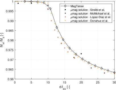
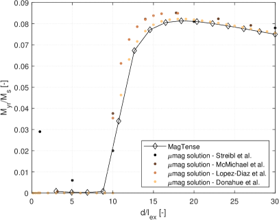
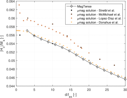
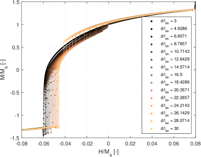
Figure 2: a) The remanent magnetization along the long axis as a function of $d/l_{\mathrm{ex}}$ and b) the remanent magnetization along the short axis as a function of $d/l_{\mathrm{ex}}$ and c) the coercivity for fields applied along the (111) direction as a function of $d/l_{\mathrm{ex}}$ and d) the computed hysteresis curves.

4.1 $\mu$mag standard problem 2

In standard problem 2, hysteresis curves must be calculated for a thin film of length $L$, width $d=L/5$ and thickness $t=d/10$. Crystalline anisotropy is neglected in this problem. An external field is applied in the [1,1,1] direction, and the magnitude of the field is slowly decreased to calculate the hysteresis curve Streibl et al. [1999]. The hysteresis loop will depend on the scaled geometry of the problem, as the scale of the thin film dimensions change relative to the length scale of the exchange interaction. The results are specified in terms of the ratio between the thin film width $d$ and the exchange length $l_{\mathrm{ex}}=\sqrt{A_{\mathrm{exch}}/K_{\mathrm{m}}}$, where $A_{\mathrm{exch}}$ is the exchange stiffness constant and $K_{\mathrm{m}}$ is the magnetostatic energy density, $K_{\mathrm{m}}=M_{\mathrm{s}}^{2}/2\mu_{0}$.

In MagTense we utilize a Cartesian mesh with the number of rectangular cuboid tiles equal to $100\times{}20\times{}3$ in the $x$-, $y$- and $z$-direction respectively. We calculate a hysteresis loop with an applied field starting at 0.08 $H/M_{\mathrm{s}}$ and decreasing the field in 4000 steps to a value of -0.08 $H/M_{\mathrm{s}}$. The micromagnetic damping parameter, $\alpha$, and the precession parameter, $\gamma$, are not specified in the problem statement. Here we take the value of $\alpha=4000$, which is close to the value for standard problem 4, while we take $\gamma=0$, as we are only interested in the final steady state configuration. At each value of the field, we evolve the magnetization 40 ns to find the new equilibrium configuration of the magnetization, before the external field is changed again. These 40 ns are sufficient to reach the equilibrium configuration for almost all cases considered. The aim is to calculate the coercivity, which is the value of the field $H_{\mathrm{c}}/M_{\mathrm{s}}$ at which the projection of the magnetization along the field is zero, and the remanence, which is the value of $\vec{M}/M_{\mathrm{s}}$ at $H_{\mathrm{a}}=0$.

It should be note that taking $\gamma=0$ is a valid approximation, even if the Landau-Lifshitz-Gilbert (LLG) equation, i.e. not the Landau-Lifshitz equation presented in Eq. 1, is considered. This is because in the limit of large damping coefficients $\alpha$ the gyromagnetic factor in the LLG scales as $\gamma/\alpha^{2}$ , whereas the damping factor scales as $\gamma/\alpha$. As the damping coefficient tends to infinity, the gyromagnetic factor then tends to 0 much faster than the damping does. Thus the apporach of using $\gamma=0$ is valid for this standard problem.

Shown in Fig. 2 is the thin film coercivity and remanence as a function of $d/l_{\mathrm{ex}}$ both for the MagTense model as well as results published in the $\mu$mag problem solutions NIS . As can be seen from the figure, the MagTense model is in agreement with the majority of the published $\mu$mag results for both the coercivity and the remanence values. In MagTense both of these values converge the slowest at low values of $d/l_{\mathrm{ex}}$. This can be seen in Fig. 2d, where at the start of the coercivity curve, at 0.08 $H/M_{\mathrm{s}}$, the simulation for the lowest $d/l_{\mathrm{ex}}$ requires a number of steps in the external field before the initial magnetization configuration has reached the correct equilibrium state. This is in line with previous results, which have demonstrated that in the small particle limit convergence can be difficult to obtain Donahue et al. [2000].

Here, the difficulty of obtaining converging at the small particle limit is most likely caused by the chosen ODE45 solver, which is not well suited to stiff problems. The demagnetization tensor approach used is correct also for length scales smaller than the exchange length, so it is not an imprecise calculation of the demagnetization field that is causing the slow convergence. An additional factor in the slow convergence at small length scales could be the chosen discretization of the finite difference exchange operator. This is chosen to be a 3-element stencil, which is correct to second order, but when the exchange coupling is strong a higher order operator may be needed. It has also previously been shown that the spatial discretization with an analytical demagnetization calculations can result in the Landau-Lifshitz equation becoming stiff Shepherd et al. [2014].

4.2 $\mu$mag standard problem 3

In standard problem 3, the goal is to calculate the minimum energy state in the single domain limit of a cubic magnetic particle of side length $L$. The standard problem consists on calculating the energy of two different states, known as the flower state and the vortex state respectively, to determine the value of $L$ at which there is a change in the minimum energy state of the cube from one of the states to the other.

The edge length of the considered cube, $L$, is similarly to standard problem 2 expressed in terms of the exchange length scale, $l_{\mathrm{ex}}=\sqrt{A_{\mathrm{exch}}/K_{\mathrm{m}}}$, where $K_{\mathrm{m}}$ is the magnetostatic energy density given by $K_{\mathrm{m}}=M_{\mathrm{s}}^{2}/2\mu_{0}$. A uniaxial anisotropy with magnitude $K_{\mathrm{u}}=0.1K_{\mathrm{m}}$ along a principal axis of the cube is assumed.

Shown in Fig. 3 is the side length in units of $l_{\mathrm{ex}}$ at which the minimum energy state switches between the flower and the vortex state as a function of resolution, i.e. the number of cubic magnetic tiles in the model. As can be seen from the figure, the crossover points approach two of the three tabulated $\mu$mag solutions as the resolution is increased. Extrapolating the energy crossover to an infinitely fine resolution by fitting a power law of $L_{\mathrm{cross}}=an^{b}+c$ to the data gives $L_{\mathrm{\infty}}=8.477\pm 0.007$, which is in line with two of the published $\mu$mag results.

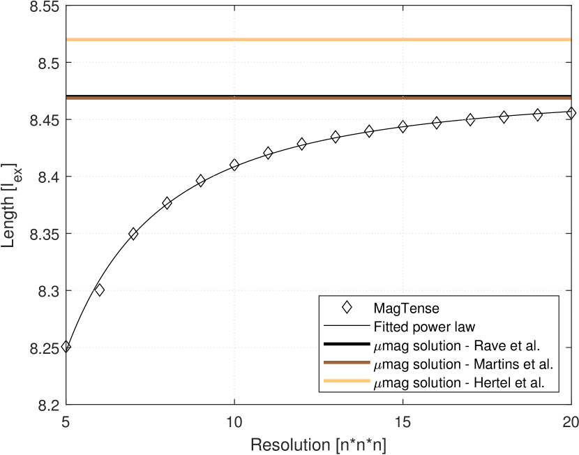
Figure 3: The side length at which the energy crossover between the flower and vortex state happens, as a function of resolution, i.e. the number of tiles, $n$, in each direction. The tabulated $\mu$mag solutions, which are extrapolated to an infinitely fine grid, are shown as well. Two of these, the Rave et al. and Martins et al. overlap.

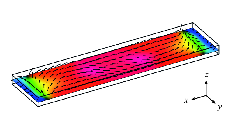
Figure 4: State of the system at an intermediate step of the relaxation process for applied field 2 in standard problem 4. The magnetization direction in each point is indicated by the black arrows and by the color. In the figure, the thickness of the film in the $z$ direction has been exaggerated for clarity.

4.3 $\mu$mag standard problem 4

In standard problem 4 the dynamic evolution of a film with a thickness of 3 nm, a length of 500 nm and a width of 125 nm is considered. We assume that the problem can be discretized in a two-dimensional grid, i.e. that the thickness is only resolved by a single tile.

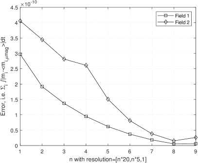
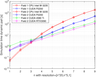
Figure 5: a) The error for standard problem 4 as defined in the text as a function of resolution and b) the computation time as a function of resolution on different hardware.

First an initial equilibrium $s$-state must be calculated, which is obtained by first applying a saturating magnetic field along the [1,1,1] direction and then slowly removing this field and letting the magnetization equilibrate. Following this one of two different magnetic fields is applied instantaneously at $t=0$ to the initial $s$-state and the time evolution of the magnetization as the system moves towards equilibrium in the new fields is simulated. The two fields considered are field 1: $\mu{}_{0}H=[-24.6,4.3,0.0]$ mT and field 2: $\mu{}_{0}H=[-35.5,-6.3,0.0]$ mT.

The parameters relevant for the problem are an exchange constant of $A_{\mathrm{exch}}=1.3\cdot 10^{-11}$ J/m, a saturation magnetization of $M_{\mathrm{s}}=8.0\cdot 10^{5}$ A/m, a damping parameter of $\alpha=4.42\cdot 10^{3}$ and a precession parameter of $\gamma=2.21\cdot 10^{5}$.

Using MagTense we compute the initial $s$-state and the following dynamical evolution for various resolutions of the uniform grid. The resolution is varied as $[20n,5n,1]$ with values of $n=1$ to $9$. Fig. 4 shows an example of magnetization distribution over the cross-section of the film. This configuration corresponds to applied field 2 after $t=0.5$ ns from the beginning of the relaxation process.

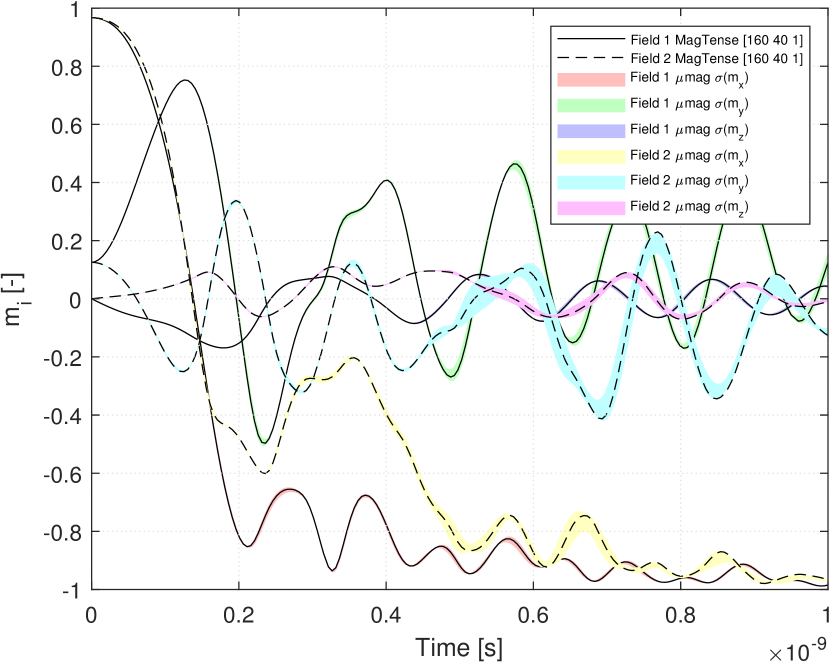
Figure 6: The three components of the magnetization as a function of time for field 1 and 2 in standard problem 4 for a resolution of [160 40 1] along with the standard deviation of the published $\mu$mag solutions.

Computing the mean of previously published models as tabulated in the $\mu$mag results, the error for the MagTense model can be defined as

$$err=\sum_{\mathrm{i}}\int_{0}^{100\mathrm{ns}}\lvert m_{\mathrm{i}}-\langle m_{\mathrm{i,\mu\mathrm{mag}}}\rangle\rvert\mathrm{d}t,$$ (18)

summing the different magnetization components and integrating over the first 100 ns of the time evolution. In Fig. 5a the error is shown as a function of resolution. As can be seen from the figure, the error decreases as the mesh resolution is increased, as expected. At a resolution of [160,40,1], i.e. $n=8$, the model has clearly converged, resulting in a minimum error between the model and the $\mu$mag tabulated data. In Fig. 5b the simulation time for the dynamic part of standard problem 4, i.e. without the calculation of the initial s-state, is shown as a function of resolution for different hardware configuration. The cases considered are a simulation where all computations are done on an Intel W-3235 CPU, as well as calculations where the demagnetization field matrix multiplications are done using CUDA on a P2200, 2080 TI and a RTX 3090 Nvidia GPU respectively. As can be seen using CUDA for the calculations results in a significant improvement in computation time, with a similar magnitude as previously seen using CUDA micromagnetic frameworks Lopez-Diaz et al. [2012]; Leliaert and Mulkers [2019].

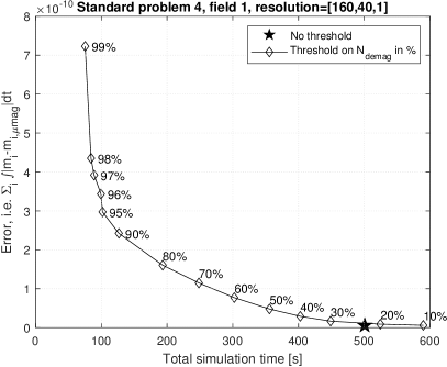
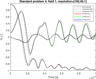
Figure 7: a) The error as a function of computation time for various threshold percentages, i.e. which percentage of the smallest values in the demagnetization tensor that is removed and b) the three components of the magnetization as a function of time for field 1 in standard problem 4 for various threshold fractions along with the standard deviation of the published $\mu$mag solutions.

The dynamic evolution of the system is shown Fig. 6 for a resolution of [160,40,1] along with the standard deviation of the published $\mu$mag solutions. As can be seen MagTense predicts an evolution that clearly is in line with the existing published $\mu$mag data.

4.3.1 Influence of thresholding the demagnetization tensor

It is of interest to explore whether or not the demagnetization tensor can be reduced in complexity from a fully dense matrix to a sparse one in order to improve the speed and memory use of the simulation. We have therefore implemented a feature in the MagTense framework such that the demagnetization tensor can be reduced in size by removing all elements of the tensor smaller than a given threshold value, i.e. all values below the threshold are truncated. This also allows the demagnetization tensor, which normally is a dense matrix, to be allocated as a sparse matrix, thus saving memory, which is especially important when doing CUDA calculations. The effect of adjusting the threshold value for the computed solution to standard problem 4 is investigated in the following.

We consider a resolution of [160,40,1]. A threshold is chosen and the values which in absolute value is smaller than the threshold is set to zero. For example for a threshold of $20\%$ the absolute smallest fifth of the elements larger than zero in the tensor is truncated to zero. In Fig. 7a the reduction in simulation time versus the error is shown for various values of the threshold, with the calculations performed on a Intel W-3235 CPU. As can be seen a reduction in computation time is possible without sacrificing accuracy. The computed dynamic solution is shown in Fig. 7b for a threshold value of 40% and 70%, respectively, to illustrate that the solution, especially for the 40% case, is still accurate compared to the tabulated $\mu$mag solutions. Note that for small values of the threshold, the calculation time increases because when a threshold is applied the demagnetization tensor is cast as a sparse matrix. When the number of elements in the tensor is still close to the fully dense matrix, there is a significant overhead in the sparse matrix multiplication of the demagnetization tensor with the magnetization, leading to the increase in simulation time.

It should be noted that thresholding the demagnetization tensor is the simplest and crudest method of reducing the number of entries in the tensor and is a technique that should be used with caution. As the magnitude of the field of a single tile decreases as $\sim 1/r^{3}$ away from the tile, this truncation strategy will in essence result in that tiles only ”see” other tiles in a more or less spherical region around themselves. This can be problematic as the number of tiles within such a sphere with radius $r$ grows as $r^{3}$, thus in effect cancelling out the $1/r^{3}$ decreasing influence of the individual tiles, making the demagnetization tensor important across the whole sample. A better but more complicated strategy for removing elements from the demagnetization tensor is to employ a multi-grid approach that scales the grid with the distance from a respective tile or use an adaptive mesh refinement technique Ramstock et al. [1996]; Hirano and Hayashi [1999]; Garcia-Cervera and Roma [2006]; Sun and Monk [2006]. Another approach is to uses different approximations for the demagnetization tensor depending on the distance to the respective tile Lebecki et al. [2008]; Krüger et al. [2013].

Another strategy could be to calculate the full demagnetization tensor and subsequently perform an FFT transformation of it and use this matrix in calculations, transforming the magnetization to Fourier-space and back in the matrix multiplication with the demagnetization tensor. For the currently used regular grids this will make the method identical to the existing FFT frameworks, but for irregular grids this may be a computationally efficient strategy.

5 Conclusion

We have presented the MagTense micromagnetic framework, which utilizes a discretization approach of tiles of either rectangular cuboid or tetrahedron geometry to analytically calculate the demagnetization field. The only assumption in this approach is that a tile is uniformly magnetized.

Using this novel approach, which differs from existing finite difference and finite element schemes, we calculated the solution to a range of the $\mu$mag standard problems in micromagnetism and showed that the MagTense framework accurately calculates the solution to each of these.

Finally, we explored the simulation time in MagTense and showed that this can be significantly improved by performing the dense demagnetization tensor matrix multiplications using CUDA, and also that the demagnetization tensor can be reduced in complexity to increase the calculation speed without significantly sacrificing the precision of the solution, albeit with possible caveats depending on the shape of the sample.

References

- Fischbacher et al. [2018] Johann Fischbacher, Alexander Kovacs, Markus Gusenbauer, Harald Oezelt, Lukas Exl, Simon Bance, and Thomas Schrefl. Micromagnetics of rare-earth efficient permanent magnets. Journal of Physics D: Applied Physics, 51(19):193002, 2018.
- Gong et al. [2019] Qihua Gong, Min Yi, and Bai Xiang Xu. Multiscale simulations toward calculating coercivity of nd-fe-b permanent magnets at high temperatures. Physical Review Materials, 3(8):084406, 2019. ISSN 24759953. 10.1103/PhysRevMaterials.3.084406.
- Kim [2010] Sang-Koog Kim. Micromagnetic computer simulations of spin waves in nanometre-scale patterned magnetic elements. Journal of Physics D: Applied Physics, 43(26):264004, 2010.
- Donahue and Porter [1999] M.J. Donahue and D.G. Porter. Oommf user’s guide, version 1.0, interagency report nistir 6376. Technical report, National Institute of Standards and Technology, Gaithersburg, MD, 1999.
- Vansteenkiste et al. [2014] Arne Vansteenkiste, Jonathan Leliaert, Mykola Dvornik, Mathias Helsen, Felipe Garcia-Sanchez, and Bartel Van Waeyenberge. The design and verification of mumax3. AIP advances, 4(10):107133, 2014.
- Leliaert et al. [2018] Jonathan Leliaert, Mykola Dvornik, Jeroen Mulkers, Jonas De Clercq, MV Milošević, and Bartel Van Waeyenberge. Fast micromagnetic simulations on gpu—recent advances made with. Journal of Physics D: Applied Physics, 51(12):123002, 2018.
- Kumar and Adeyeye [2017] D Kumar and AO Adeyeye. Techniques in micromagnetic simulation and analysis. Journal of Physics D: Applied Physics, 50(34):343001, 2017.
- Abert et al. [2013] Claas Abert, Lukas Exl, Gunnar Selke, André Drews, and Thomas Schrefl. Numerical methods for the stray-field calculation: A comparison of recently developed algorithms. Journal of Magnetism and Magnetic Materials, 326:176–185, 2013.
- Van de Wiele et al. [2008] Ben Van de Wiele, Femke Olyslager, and Luc Dupré. Application of the fast multipole method for the evaluation of magnetostatic fields in micromagnetic computations. Journal of Computational Physics, 227(23):9913–9932, 2008.
- Palmesi et al. [2017] Pietro Palmesi, Lukas Exl, Florian Bruckner, Claas Abert, and Dieter Suess. Highly parallel demagnetization field calculation using the fast multipole method on tetrahedral meshes with continuous sources. Journal of Magnetism and Magnetic Materials, 442:409–416, 2017.
- Vansteenkiste and Van de Wiele [2011] Arne Vansteenkiste and Ben Van de Wiele. Mumax: A new high-performance micromagnetic simulation tool. Journal of Magnetism and Magnetic Materials, 323(21):2585–2591, 2011.
- Ferrero and Manzin [2020] Riccardo Ferrero and Alessandra Manzin. Adaptive geometric integration applied to a 3d micromagnetic solver. Journal of Magnetism and Magnetic Materials, page 167409, 2020.
- Livshitz et al. [2009] Boris Livshitz, Amir Boag, H Neal Bertram, and Vitaliy Lomakin. Nonuniform grid algorithm for fast calculation of magnetostatic interactions in micromagnetics. Journal of Applied Physics, 105(7):07D541, 2009.
- Exl and Schrefl [2014] Lukas Exl and Thomas Schrefl. Non-uniform fft for the finite element computation of the micromagnetic scalar potential. Journal of Computational Physics, 270:490–505, 2014.
- Lepadatu [2019] Serban Lepadatu. Efficient computation of demagnetizing fields for magnetic multilayers using multilayered convolution. Journal of Applied Physics, 126(10):103903, 2019.
- Exl et al. [2012] Lukas Exl, Winfried Auzinger, Simon Bance, Markus Gusenbauer, Franz Reichel, and Thomas Schrefl. Fast stray field computation on tensor grids. Journal of computational physics, 231(7):2840–2850, 2012.
- J. García-Cervera [2014] Carlos J. García-Cervera. Numerical micromagnetics: A review. Boletin de la Sociedad Espanola de Matematica Aplicada, 39:130–135, 2014.
- Rotarescu et al. [2019] C. Rotarescu, H. Chiriac, N. Lupu, and T. A. Óvári. Micromagnetic analysis of magnetization reversal in fe77.5si7.5b15 amorphous glass-coated nanowires. Aip Advances, 9(10):105316, 2019. ISSN 21583226. 10.1063/1.5119450.
- Perez et al. [2014] Noel Perez, Luis Torres, and Eduardo Martinez-Vecino. Micromagnetic modeling of dzyaloshinskii–moriya interaction in spin hall effect switching. Ieee Transactions on Magnetics, 50(11):1–4, 2014. ISSN 19410069, 00189464. 10.1109/TMAG.2014.2323707.
- Ragusa et al. [2009] C. Ragusa, M. D’Aquino, C. Serpico, B. Xie, M. Repetto, G. Bertotti, and D. Ansalone. Full micromagnetic numerical simulations of thermal fluctuations. Ieee Transactions on Magnetics, 45(10):5257303, 3919–3922, 2009. ISSN 19410069, 00189464. 10.1109/TMAG.2009.2021856.
- Smith et al. [2010] Anders Smith, Kaspar Kirstein Nielsen, DV Christensen, Christian Robert Haffenden Bahl, Rasmus Bjørk, and J Hattel. The demagnetizing field of a nonuniform rectangular prism. Journal of Applied Physics, 107(10):103910, 2010.
- Nielsen et al. [2019] Kaspar Kirstein Nielsen, Andrea Roberto Insinga, and Rasmus Bjørk. The stray- and demagnetizing field from a homogeneously magnetized tetrahedron. I E E E Magnetics Letters, 10:8918242, 2019. ISSN 19493088, 1949307x. 10.1109/LMAG.2019.2956895.
- Sozer et al. [2014] Emre Sozer, Christoph Brehm, and Cetin C. Kiris. Gradient calculation methods on arbitrary polyhedral unstructured meshes for cell-centered cfd solvers. 52nd Aiaa Aerospace Sciences Meeting - Aiaa Science and Technology Forum and Exposition, Scitech 2014, pages 24 pp., 24 pp., 2014. 10.2514/6.2014-1440.
- Insinga et al. [2020] A.R. Insinga, E. Blaabjerg Poulsen, K.K. Nielsen, and R. Bjørk. A direct method to solve quasistatic micromagnetic problems. Journal of Magnetism and Magnetic Materials, 510:166900, 2020. ISSN 18734766, 03048853. 10.1016/j.jmmm.2020.166900.
- Lopez-Diaz et al. [2012] L Lopez-Diaz, D Aurelio, L Torres, E Martinez, MA Hernandez-Lopez, J Gomez, O Alejos, M Carpentieri, G Finocchio, and G Consolo. Micromagnetic simulations using graphics processing units. Journal of Physics D: Applied Physics, 45(32):323001, 2012.
- Leliaert and Mulkers [2019] Jonathan Leliaert and Jeroen Mulkers. Tomorrow’s micromagnetic simulations. Journal of Applied Physics, 125(18):180901, 2019.
- Bjørk and Nielsen [2019] R Bjørk and K. K. Nielsen. Magtense - a micromagnetism and magnetostatic framework. doi.org/10.11581/DTU:00000071, https://www.magtense.org, 2019.
- Krüger et al. [2013] Benjamin Krüger, Gunnar Selke, André Drews, and Daniela Pfannkuche. Fast and accurate calculation of the demagnetization tensor for systems with periodic boundary conditions. IEEE transactions on magnetics, 49(8):4749–4755, 2013.
- Lebecki et al. [2008] Krzysztof M Lebecki, Michael J Donahue, and Marek W Gutowski. Periodic boundary conditions for demagnetization interactions in micromagnetic simulations. Journal of Physics D: Applied Physics, 41(17):175005, 2008.
- Moskowitz and Della Torre [1966] R Moskowitz and E Della Torre. Theoretical aspects of demagnetization tensors. IEEE Transactions on Magnetics, 2(4):739–744, 1966.
- [31] mag standard problems, accessed on november 1st, 2020. URL https://www.ctcms.nist.gov/~rdm/toc.html.
- Streibl et al. [1999] B Streibl, T Schrefl, and J Fidler. Dynamic fe simulation of mag standard problem no. 2. Journal of applied physics, 85(8):5819–5821, 1999.
- Donahue et al. [2000] Michael J Donahue, Donald G Porter, Robert D McMichael, and J Eicke. Behavior of mag standard problem no. 2 in the small particle limit. Journal of Applied Physics, 87(9):5520–5522, 2000.
- Shepherd et al. [2014] David Shepherd, Jim Miles, Matthias Heil, and Milan Mihajlović. Discretization-induced stiffness in micromagnetic simulations. IEEE Transactions on Magnetics, 50(11):1–4, 2014.
- Ramstock et al. [1996] Klaus Ramstock, Alex Hubert, and D Berkov. Techniques for the computation of embedded micromagnetic structures. IEEE Transactions on Magnetics, 32(5):4228–4230, 1996.
- Hirano and Hayashi [1999] Satoshi Hirano and Nobuo Hayashi. Multigrid computation for micromagnetics. Journal of applied physics, 85(8):6205–6207, 1999.
- Garcia-Cervera and Roma [2006] Carlos J Garcia-Cervera and Alexandre M Roma. Adaptive mesh refinement for micromagnetics simulations. IEEE transactions on magnetics, 42(6):1648–1654, 2006.
- Sun and Monk [2006] Jiguang Sun and Peter Monk. An adaptive algebraic multigrid algorithm for micromagnetism. IEEE transactions on magnetics, 42(6):1643–1647, 2006.