Structured Directional Pruning

Abstract

Structured pruning is an effective compression technique to reduce the computation of neural networks, which is usually achieved by adding perturbations to reduce network parameters at the cost of slightly increasing training loss. A more reasonable approach is to find a sparse minimizer along the flat minimum valley found by optimizers, i.e. stochastic gradient descent, which keeps the training loss constant. To achieve this goal, we propose the structured directional pruning based on orthogonal projecting the perturbations onto the flat minimum valley. We also propose a fast solver AltSDP and further prove that it achieves directional pruning asymptotically after sufficient training. Experiments using VGG-Net and ResNet on CIFAR-10 and CIFAR-100 datasets show that our method obtains the state-of-the-art pruned accuracy (i.e. 93.97% on VGG16, CIFAR-10 task) without retraining. Experiments using DNN, VGG-Net and WRN28$\times$10 on MNIST, CIFAR-10 and CIFAR-100 datasets demonstrate our method performs structured directional pruning, reaching the same minimum valley as the optimizer.

1 Introduction

Deep Neural Network (DNN) has developed rapidly in recent years owing to its state-of-the-art performance in various domains [1, 2, 3]. The development of DNN involves some heuristics, such as the use of deeper and more extensive models, which is also a development trend in recent years [4, 5]. These heuristics enhance the expressive ability of neural networks by overparameterization [6], however, in turn, restricting their usage on resource-limited devices, such as mobile phones, autonomous cars and augmented reality devices. This has prompted technological developments in shrinking DNN while maintaining accuracy.

Sparse DNN is a representative algorithm for shrinking DNN, which is popular since it requires less memory and storage capacity and reduces inference time [7]. Here, sparse neural networks refer to neural networks with most parameters of zero. Magnitude pruning is an effective way to obtain sparse DNNs [7, 8, 9, 10, 11]. Magnitude pruning is divided into unstructured pruning (fine-grained pruning) [7, 8, 12] and structured pruning (coarse-grained pruning) [9, 10, 11] according to whether the structure of neural networks is used. Unstructured pruning directly prunes weights independently in each layer to achieve higher sparsity. However, it usually requires dedicated hardware or software accelerators to accelerate access to irregular memory, which affects the efficiency of online reasoning [11]. In contrast, structured pruning does not require dedicated hardware/software packages, as it only removes structured weights (including 2D kernels, filters, or layers) and does not yield irregular memory accesses.

Unfortunately, structured pruning still suffers some open issues. After removing the entire structure of the network, retraining or fine tuning is needed for better performance [9], which requires extra effort and more intensive computing [10]. Moreover, these structured pruning methods are typically tailored to specific network structures, such as filters or kernels, and cannot be flexibly applied to heterogeneous structures [11]. In this paper, we propose a general structured directional pruning (SDP) scheme based on perturbation orthogonal projection to solve the above problems, which does not require fine tuning or retraining. Group lasso regularization, which has shown excellent performance in areas such as compressed sensing, online learning and tiny AI [13, 14, 15], is adopted to explore structural sparsity in neural networks. Subsequently, the perturbations caused by sparse regularization are orthogonally projected onto a plane with constant loss function values. Using the projected perturbation to update the network eliminates the need for fine tuning and retraining, since the accuracy of the network is not compromised. Moreover, the technique can be flexibly applied to heterogeneous structures as it can prune different structures simultaneously.

1.1 Contributions

In this paper, we propose a general structured pruning scheme for directional pruning of neural networks, which reaches the flat minimum valley found by optimizers, such as stochastic gradient descent (SGD), when pruning. In particular, we orthogonally project the sparse perturbations onto a constant loss value plane and update the network accordingly. Hence, our structured directional pruning suppresses only the unimportant parameters and encourages the important ones simultaneously, while traditional structured pruning methods tend to suppress all parameters, resulting in performance losses.

In addition, a fast implementation solver, named alternating structured directional pruning (AltSDP) algorithm, based on regularized dual averaging is proposed, which can quickly adjust the weights on each structural unit to achieve orthogonal projection. Moreover, we further theoretically prove that AltSDP achieves the effect of the structured directional pruning after sufficient training.

We optimize the implementation of the proposed algorithm so that it can be combined with many optimizers and algorithms (for example stochastic gradient descent (SGD) and SGD with momentum algorithm) in the deep learning framework, e.g. Tensorflow or PyTorch. This allows our algorithm to achieve optimal pruning performance on a wide range of datasets and networks. Experiments using VGG-Net and ResNet on CIFAR-10 and CIFAR-100 datasets show that our method obtains the state-of-the-art pruned accuracy (e.g. 93.97% on VGG16, CIFAR-10 task) without retraining. Experiments using DNN, VGG-Net and WRN28$\times$10 on MNIST, CIFAR-10 and CIFAR-100 datasets demonstrate our method performs structured directional pruning, reaching the same minimum valley as the optimizer.

1.2 Related Works

Structured pruning: In [16], a network slimming method based on the channel-level sparsity was proposed to automatically identify and prune insignificant channels. In [17], a channel pruning method was proposed via a LASSO regression based channel selection and least square reconstruction. AutoML for model compression was proposed in [18], which utilizes reinforcement learning to improve the model compression quality. Discrimination-aware channel pruning was proposed in [19] to choose channels that significantly contribute to discriminative power. In  [20], the soft filter pruning was proposed to inference procedure of deep convolutional neural networks, which has larger model capacity and less dependence on the pre-trained model. Filter pruning via geometric median was proposed in [21], which improves pruning performance in the cases where “smaller-norm-less-important” criterion does not hold. In addition, collaborative channel pruning was proposed in [22] to reduce the computational overhead of deep networks. Polarization regularizer was proposed in [23] to suppress only unimportant neurons while keeping important neurons intact. Moreover, correlation-based pruning was proposed in [24], which utilizes parameter-quantity and computational-cost regularization terms to enable the users to customize the compression according to their preference. Unfortunately, the above methods still suffer from a loss of accuracy when pruning. Retraining and fine-tuning are hard to avoid, which requires extra effort and more intensive computing.

Directional pruning: Directional pruning is first proposed in [7], which searches for a sparse minimizer in or close to the flat minimum valley in training loss obtained by the stochastic gradient descent. Retraining or the expert knowledge on the sparsity level is no longer needed. This work motivates us to propose structured directional pruning. However, extending directional pruning to structured directional pruning is not straightforward. Since the algorithm and theoretic analysis have major differences when the sparse $\ell_{1}$-norm regularization is replaced by the group LASSO regularization.

2 Structured Directional Pruning

2.1 Structured Pruning

Considering a deep neural network with overparameterization ${\bm{w}}\in\mathbb{R}^{d}$, the structured pruning aims to eliminate redundant parameters in ${\bm{w}}$ structurally, which can be formulated as

$$\arg\min_{{\bm{w}}}\|{\bm{w}}^{\star}-{\bm{w}}\|_{2}^{2}+\mathcal{S}({\bm{w}},\mathcal{G}),$$ (1)

where ${\bm{w}}^{\star}$ denotes a minimizer of the model parameters satisfying $\nabla\ell({\bm{w}}^{\star})=0$ with $\ell:\mathbb{R}^{d}\rightarrow\mathbb{R}$ being the loss function; $\mathcal{G}$ is a structured partition of $\{1,2,\dots,d\}$ that used to divide/structure ${\bm{w}}$ into $|\mathcal{G}|$ groups or vectors, e.g., $\mathcal{G}=\{\{1,2,3\},\cdots,\{d-1,d\}\}$; ${\mathcal{S}}$ is a sparse regularization, e.g., $\ell_{0}$ norm, to utilize the structured sparsity of parameters according to $\mathcal{G}$. Taking the group lasso regularization as an example, (1) reduces to

$$\arg\min_{{\bm{w}}}\|{\bm{w}}^{\star}-{\bm{w}}\|_{2}^{2}+\sum_{i=1}^{|\mathcal{G}|}\lambda\|{\bm{w}}_{i}\|_{2},$$ (2)

where $\lambda>0$ is a weight factor; ${\bm{w}}_{i}$ is the $i$-th group coefficients of ${\bm{w}}$ for $i\in[1,\cdots,|\mathcal{G}|]$ . We can change $\mathcal{G}$ to achieve different sparse structure, e.g., filter-level sparsity, kernel-level sparsity and vector-level sparsity. And if $|\mathcal{G}|=d$ with $\mathcal{G}=\{\{1\},\{2\},\cdots,\{d\}\}$, the structured pruning reduces to non-structured pruning or fine-grained pruning, which prunes weights irregularly.

Note that, the sparse regularization in (2) penalizes all ${\bm{w}}_{i}$ to realize structured pruning, which may increase training loss while pruning. Figure 1 (left) demonstrates this limitation intuitively, in which the dark blue region contains all possible case for traditional structured pruning. To solve this problem, we propose the structured directional pruning in the next subsection.

2.2 SDP: Problem Formulation

Structured directional pruning tends to prune the neural network along the direction that does not change the training loss. The idea behind is first to find a subspace, called $\mathcal{P}$ (red subspace in Figure. 1), where the training loss is fixed, and then project the sparse perturbation onto it. The network is updated with the perturbation after projection to keep the training loss constant.

To find ${\mathcal{P}}$, we first analysis the local geometry of the loss function through its Hessian matrix. Since $\nabla f({\bm{w}}^{\star})\approx 0$, the Hessian $\nabla^{2}\ell({\bm{w}}^{\star})$ has multiple nearly zero eigenvalues [25, 26]. According to the second Taylor expansion of $\ell({\bm{w}}^{\star})$, the training loss will be almost constant when pruning in directions related to these eigenvalues. This means that the subspace $\mathcal{P}$ can be generated based on these directions. Note that, traditional structured pruning (the purple vector in Figure 1) is difficult to prune networks along $\mathcal{P}$, since it is nearly orthogonal to ${\bm{w}}^{\star}$ [25], which may reveal why traditional structured pruning requires fine tuning or retraining.

To prune ${\bm{w}}^{\star}$ along $\mathcal{P}$, inspired by the directional pruning [7], we first introduce direction factors $s_{i},i=1,\cdots,|\mathcal{G}|$, which reflects the angle between ${\bm{w}}_{i}$ and ${\Pi}_{i}({\bm{w}}^{\star})$, where ${\Pi}(\cdot)$ represents an operator of projecting the input vector onto the subspace $\mathcal{P}$, and ${\Pi}_{i}(\cdot)$ denotes its $i$-th group that is separated w.r.t. $\mathcal{G}$. Different from (2), structured directional pruning, defined in Definition 1, decrease the magnitude of ${\bm{w}}_{i}^{\star}$ with $s_{i}>0$ (acute angle) and simultaneously increase the magnitude of ${\bm{w}}_{i}^{\star}$ with $s_{i}<0$ (obtuse angle).

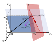
(a)

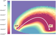
(b)

Figure 1: Left: a 3D graphical illustration of the structured pruning, where ${\bm{w}}^{\star}=(w_{1},w_{2},w_{3})$ with $\mathcal{G}=\{\{1,2\},\{3\}\}$. The dark blue region contains all possible directions of traditional structured pruning, while the red dashed line contains directions of structured directional pruning with different $\lambda$, which is the orthogonal projection of traditional directions onto the constant loss value plane ${\mathcal{P}}$ (red). Right: the contour of the training loss on CIFAR10, VGG16 task around the solutions found by AltSDP (the algorithm we propose to achieve SDP) and SGD ($\bm{w}^{*}$). The white curve can be understood as the red dashed line in the left figure, while the dark red region can be understood as the plane ${\mathcal{P}}$.

Definition 1.

(Structured directional pruning). Suppose that ${\bm{w}}^{\star}\in\mathbb{R}^{d}$ is a minimizer satisfies $\nabla\ell({\bm{w}}^{\star})=0$ with $\ell(\cdot)$ being the loss function. Assume that none of the coefficients in ${\bm{w}}^{\star}$ is zero. The structured directional pruning is given by

$$\arg\min_{{\bm{w}}}\frac{1}{2}\|{\bm{w}}^{\star}-{\bm{w}}\|_{2}^{2}+\lambda\sum_{i=1}^{|\mathcal{G}|}s_{i}\|{\bm{w}}_{i}\|_{2},$$ (3)

where $\lambda>0$ is a weight factor, $\mathcal{G}$ is the structured partition, and $s_{i}$ is the direction factor

$$s_{i}:=\left\langle E({\bm{w}}_{i}^{\star}),{\Pi}_{i}(E_{\mathcal{G}}({\bm{w}}^{\star}))\right\rangle>0$$ (4)

with $\langle\cdot\rangle$ being the inner product, $E(\cdot)$ being the normalization operator, i.e., $E({\bm{w}})={\bm{w}}/\|{\bm{w}}\|_{2}$, and $E_{\mathcal{G}}(\cdot)$ being the normalization operator w.r.t. $\mathcal{G}$, i.e., $E_{\mathcal{G}}({\bm{w}})=[E({\bm{w}}_{1})^{T},E({\bm{w}}_{2})^{T},...,E({\bm{w}}_{|\mathcal{G}|})^{T}]^{T}$.

Our structured directional pruning can also be understood as being based on the orthogonal projection of perturbations. That is, structured pruning $\bm{w}^{\star}$ in (1) can be rewritten as a perturbation of $\bm{w}^{\star}$, i.e.,

$$\bm{w}_{i}^{\star}-\xi_{i}E(\bm{w}_{i}^{\star}),~{}i=1,...,|\mathcal{G}|,$$ (5)

where $0\leq\xi_{i}\leq\|\bm{w}_{i}^{\star}\|_{2}$ and the $i$-th group of $\bm{w}^{\star}$ is pruned if $\xi_{i}=\|\bm{w}_{i}^{\star}\|_{2}$. Since usually $[\xi_{1}E({\bm{w}}_{1}^{\star})^{T},\xi_{2}E({\bm{w}}_{2}^{\star})^{T},...,\xi_{|\mathcal{G}|}E({\bm{w}}_{|\mathcal{G}|}^{\star})^{T}]^{T}\notin\mathcal{P}$, retraining is need for traditional structured pruning. By comparision, our SDP can be viewed as pruning $\bm{w}^{\star}$ by setting $\xi_{i}=\lambda s_{i}$, then we have $\bm{w}_{i}^{\star}-\lambda{\Pi}_{i}(E_{\mathcal{G}}({\bm{w}}^{\star})),~{}i=1,...,|\mathcal{G}|$ by noting that $s_{i}E(\bm{w}_{i}^{\star})={\Pi}_{i}(E_{\mathcal{G}}({\bm{w}}^{\star}))$, i.e., pruning along $\mathcal{P}$ by using the orthogonal projection of perturbations.

2.3 Difference from Directional Pruning

For comparison, we briefly present directional pruning [7], which prunes weights one by one as follows

$$\arg\min_{{\bm{w}}}\frac{1}{2}\|{\bm{w}}^{\star}-{\bm{w}}\|_{2}^{2}+\lambda\sum_{j=1}^{d}s_{j}^{\rm d}|{w}_{j}|,$$ (6)

where ${w}_{j}$ denotes the $j$-th element in $\bm{w}$ and

$$s_{j}^{\rm d}:={\rm sign}({w}_{j}^{\star})\cdot({\Pi}^{\rm d}\{{\rm sign}({\bm{w}}^{\star})\})_{j}>0,$$ (7)

where ${\Pi}^{\rm d}(\cdot)$ represents the operator of projecting the input vector onto the subspace $\mathcal{P}^{\rm d}$, where the training loss in (6) is fixed. Obviously, our SDP and directional pruning have the following differences:

• SDP uses regularization based on group LASSO, while directional pruning uses that based on $\ell_{1}$-norm;

• In (7), we only need to calculate one projection ${\Pi}^{\rm d}(\cdot)$. In contrast, SDP introduces different grouping structures, and each group has its own different projection operator ${\Pi}_{i}(\cdot)$. Calculating them simultaneously makes the problem more complicated;

• The vector ${\rm sign}({\bm{w}}^{\star})$ is on the vertices of the unit hypercube, while $E_{\mathcal{G}}({\bm{w}}^{\star})$ is on the unit hypersphere. It is more difficult to project a vector on the unit hypersphere onto ${\mathcal{P}}$, since the number of vectors on it is far more than that on the vertices of the unit hypercube;

• We obtain $s_{j}^{\rm d}$ in (7) by performing magnitude correction on the sign of $w_{j}$, while we obtain $s_{i}$ in (4) by calculating the inner product between two normalized vectors and limiting the angle between them to be an acute angle, i.e., the inner product is greater than 0.

The above differences make the solutions of SDP and directional pruning different, and also make the corresponding solvers different. We will propose the SDP solution and the corresponding fast solver in the next section.

3 Algorithm & Theoretical Analysis

In this section, we first present the optimal solution of the structured directional pruning in (3). Since it is computationally unfriendly to neural networks, we then propose its fast solver, and further prove that the proposed solver can asymptotically achieve the effect of structured directional pruning under some reasonable assumptions.

3.1 Algorithm

To start with, since the objective function in (3) is separable for each group/structure, we propose the following Theorem 1 to demonstrate that each subproblem has an explicit solution.

Theorem 1.

Consider the optimization problem

$$\arg\min_{{\bm{w}}_{i}}\left\{\frac{1}{2}\|{\bm{w}}_{i}^{\star}-{\bm{w}}_{i}\|_{2}^{2}+\lambda{s}_{i}\|{\bm{w}}_{i}\|_{2}\right\}.$$ (8)

For ${\bm{w}}_{i}^{\star}\in\mathbb{R}^{d}\backslash\{\bm{0}\},{s}_{i}\in\mathbb{R},\lambda>0$, (8) has an explicit solution:

$$\hat{\bm{w}}_{i}=\left(1-\frac{\lambda{s}_{i}}{\|{\bm{w}}_{i}^{\star}\|_{2}}\right)_{+}{\bm{w}}_{i}^{\star}.$$ (9)

The above theorem gives the solution to the subproblem of (3), which is proved in Appendix. Since the original problem is a superposition of subproblems, i.e., the above problem indirectly elucidates the solution of directional pruning. However, determining $s_{i}$ in Theorem 1 requires computing the Hessian $\nabla^{2}\ell({\bm{w}}^{\star})$ to find $\mathcal{P}_{0}$, which is computationally cumbersome. We hence propose a fast solver by alternating minimization, named AltSDP, to asymptotically obtain the structural sparse model in the following. The idea behind is to separate the progress of finding the optimal ${\bm{w}}^{\star}$ and its sparse structure through an alternative manner.

Considering an overparameterized DNN with training data $Z_{i}=\left\{(X_{i},Y_{i})\right\}_{i=1}^{N}$ and parameters ${\bm{w}}\in\mathbb{R}^{d}$. Assume that $h(x;\bm{w})$ is the network output, denote $f(\bm{w};Z):=\mathcal{L}(h(X;\bm{w});Y)$ with $\mathcal{L}(h;y)$ being a loss function, e.g. the cross-entropy loss or the mean squared error (MSE) loss. And let $\nabla f({\bm{w}},Z)$ be the gradient of $f({\bm{w}},Z)$ w.r.t. ${\bm{w}}$. To this end, our AltSDP is given by

$${\bm{v}}_{n+1} ={\bm{v}}_{n}-\gamma\nabla f({\bm{w}}_{n};{Z}_{n+1})$$ (AltSDP-(a))

$${\bm{w}}_{n+1} =\arg\min_{{\bm{w}}\in\mathbb{R}^{d}}\Big{\{}\frac{1}{2}\|{\bm{w}}\|_{2}^{2}-{\bm{w}}^{T}{\bm{v}}_{n+1}$$

$$~{}~{}~{}~{}~{}~{}~{}~{}~{}~{}~{}~{}~{}~{}~{}~{}~{}~{}~{}+g(n,\gamma)\sum_{i=1}^{|\mathcal{G}|}\|{\bm{w}}_{i}\|_{2}\Big{\}},$$ (AltSDP-(b))

where $n=0,1,\cdots$ is the iteration number; $Z_{n+1}\in Z$ is the $n$-th training data; $g(n,\gamma)=c\sqrt{\gamma}(n\gamma)^{\mu}$ is the tuning function movitated by [27] with $c,\mu>0$ being two hyperparameters that control the strength of penalization. The iteration of AltSDP can be easily started with a random initialization ${\bm{w}}_{0}$. Note that, following the proof of Theorem 1, we can have the solution of (AltSDP-(b)), i.e., for each $i\in[1,...,|\mathcal{G}|]$, we have

$${\bm{w}}_{n+1,i}=\left(1-\frac{g(n,\gamma)}{\|{\bm{v}}_{n+1,i}\|_{2}}\right)_{+}{\bm{v}}_{n+1,i}.$$ (10)

Remark 1.

Following the analysis in [27, 28], it shows that $g(n,\gamma)$ is the most important part to achieve the structured directional pruning, where $(n\gamma)^{\mu}$ is used to match the growing magnitude of (AltSDP-(a)). If $g(n,\gamma)=n\gamma$ and ${\bm{w}}_{0}=0$, our AltSDP reduces to the group lasso based regularized dual averaging (RDA) algorithm [29], and no longer has structured directional pruning ability.

3.2 Theoretical Analysis

In this subsection, we show AltSDP achieves the structured directional pruning asymptotically based on the stochastic gradient descent, i.e., under the condition that $\bm{w}^{\star}=\bm{w}^{SGD}$. Denote $G({\bm{w}}):=\nabla\ell({\bm{w}}):=\mathbb{E}_{\mathcal{Z}}[\nabla f(\bm{w};Z)]$, where $\mathbb{E}_{\mathcal{Z}}[\nabla f(\bm{w},Z)]=1/N\sum_{i=1}^{N}f(\bm{w};Z_{i})$. Define $\Sigma({\bm{w}}):=\mathbb{E}_{\mathcal{Z}}\left[(\nabla f({\bm{w}};Z)-\nabla\ell({\bm{w}}))(\nabla f({\bm{w}};Z)-\nabla\ell({\bm{w}}))^{T}\right].$ Define the gradient flow ${\bm{w}}(t)$ to be the solution of the ordinary differential equation (ODE)

$$\dot{{\bm{w}}}=-G({\bm{w}}),{\bm{w}}(0)={\bm{w}}_{0},$$ (11)

where ${\bm{w}}_{0}$ is a random initializer. It is known that $\bm{w}(t)$ can find a good global minimizer under various conditions [30]. Hence, we assume the solution of (11) is unique.

Let $H(\cdot):=\mathbb{E}_{\mathcal{Z}}[\nabla^{2}f(\cdot;Z)]$ be the Hessian matrix, and $\Phi(t,s)$ be the principal matrix solution of the matrix ODE system [31]:

$$\frac{d\Phi(t,s)}{dt}=-H({\bm{w}}(t))\Phi(t,s),\quad\Phi(s,s)=I_{d}.$$ (12)

Define ${\bm{w}}_{\gamma}(t):={\bm{w}}_{\left\lfloor t/\gamma\right\rfloor}$, where $\left\lfloor x\right\rfloor$ denotes the greatest integer not greater than $x$. Then, we make the following reasonable assumptions.

Assumption 1.

$\nabla\ell({\bm{w}}):\mathbb{R}^{d}\rightarrow\mathbb{R}^{d}$ is continuous on $\mathbb{R}^{d}$.

Assumption 2.

$\Sigma({\bm{w}}):\mathbb{R}^{d}\rightarrow\mathbb{R}^{d\times d}$ is continuous, and $\mathbb{E}_{\mathcal{Z}}[\sup_{\|{\bm{w}}\|\leq K}\|\nabla f({\bm{w}},Z)]<\infty$ a.s. for any $K$.

Assumption 3.

The Hessian matrix $H({\bm{w}}):\mathbb{R}^{d}\rightarrow\mathbb{R}^{d\times d}$ is continuous.

Assumption 4.

There exists a non-negative definite matrix $\bar{H}$ such that $\int_{0}^{\infty}\|H({\bm{w}}(s))-\bar{H}\|ds\leq\infty$ with $\|\cdot\|$ being the spectral norm, and the eigenspace of $\bar{H}$ associated with zero eigenvalues matches the subspace $\mathcal{P}$.

Assumption 5.

${c\int_{0}^{t}\Phi(t,s)\frac{\partial E_{\mathcal{G}}({\bm{w}}(s))s^{\mu}}{\partial s}ds={o}(t^{\mu})}$, where $E_{\mathcal{G}}({\bm{w}}(t))$ is defined in (4).

Assumption 6.

There exists $\bar{T}>0$, such that $E_{\mathcal{G}}({\bm{w}}(t))=E_{\mathcal{G}}({\bm{w}}^{SGD}(t))=E_{\mathcal{G}}({\bm{w}}(\bar{T}))$ a.s. for $t>\bar{T}$.

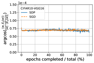
Figure 2: The angle between $\bm{w}(t)$ and ${E_{\mathcal{G}}({\bm{w}}(t))}$.

Note that the above assumptions hold empirically and strictly under some conditions. We explain in detail in the remarks below. Next, we propose Theorem 2 to show that AltSDP achieves the structured directional pruning asymptotically, which is proved in Appendix.

Remark 2.

(Condition (A4)). This condition can be verified on some simple networks under the MSE loss. It is known that once $\bm{w}(t)$ and SGD converge to the same flat valley of minima, the subspace $\mathcal{P}$ matches the eigenspace of $\bar{H}$ associated with the zero eigenvalues [7]. In addition, [32, 33] showed that $\bm{w}(t)\rightarrow\bm{w}^{\star}$ for one hidden layer networks under the teacher-student framework and MSE loss, then the limit $\bar{H}=H(\bm{w}^{\star})$ and the condition holds.

Remark 3.

(Condition (A5)). This assumption can be understood as that ${E_{\mathcal{G}}({\bm{w}}(t))}$ is assumed to be mainly restricted in the eigenspace of $H(\bm{w}(t))$ associated with positive eigenvalues as $t\rightarrow\infty$. Since [34, 25] proved that $\bm{w}(t)$ lies mainly in the subspace of $H(\bm{w}(t))$ associated with positive eigenvalues, and Figure 2 shows that the angle between $\bm{w}(t)$ and ${E_{\mathcal{G}}({\bm{w}}(t))}$ is very small, we can conclude that this assumption holds empirically.

Remark 4.

(Condition (A6)). For the MSE loss, we have $\bm{w}(t)\rightarrow\bm{w}^{\star}$ under some conditions according to Remark 2, hence $E_{\mathcal{G}}({\bm{w}}(t))=E_{\mathcal{G}}({\bm{w}}(\bar{T}))$ holds. For the cross-entropy loss, [29, 35] proved that $\bm{w}(t)/\|\bm{w}(t)\|_{2}$ converges to a unique direction when $\|\bm{w}(t)\|_{2}\rightarrow\infty$, which shows that $E_{\mathcal{G}}({\bm{w}}(t))$ stabilizes after a finite time and hence we have $E_{\mathcal{G}}({\bm{w}}(t))=E_{\mathcal{G}}({\bm{w}}(\bar{T}))$ holds. In addition, if $\gamma\rightarrow 0$, the deviation between the gradient flow and the SGD is small, and hence $E_{\mathcal{G}}({\bm{w}}(t))=E_{\mathcal{G}}({\bm{w}}^{SGD}(t))$ holds.

Dataset	Model	Method	Baseline	Pruned
			Acc. (%)	Acc. (%)	Acc.	FLOPs
					Drop (%)	Reduction
CIFAR-10	ResNet-56	NS [16] (New)	93.80	93.27	0.53	48%
		CP [17]	92.80	91.80	1.00	50%
		AMC [18]	92.80	91.90	0.90	50%
		DCP [19]	93.80	93.49	0.31	50%
		DCP-adapt [19]	93.80	93.81	-0.01	47%
		SFP [20]	93.59	93.35	0.24	51%
		FPGM [21]	93.59	93.49	0.10	53%
		CCP [22]	93.50	93.46	0.04	47%
		DeepHoyer [22]	93.80	93.54	0.26	48%
		PR [23]	93.80	93.83	-0.03	47%
		Ours	93.80	93.90	-0.10	55%
	VGG-16	NS [16] (New)	93.88	93.62	0.26	51%
		FPGM [21]	93.58	93.54	0.04	34%
		PR [23]	93.88	93.92	-0.04	54%
		Ours	93.88	93.97	-0.09	55%
CIFAR-100	ResNet-56	NS [16] (New)	72.49	71.40	1.09	24%
		PR [23]	72.49	72.46	0.06	25%
		Ours	72.49	72.55	-0.06	24%
	VGG-16	NS [16] (New)	73.83	74.20	-0.37	38%
		COP [24]	72.59	71.77	0.82	43%
		PR [23]	73.83	74.25	-0.42	43%
		Ours	73.83	74.29	-0.46	43%

Table 1: Results on CIFAR-10 and CIFAR-100. Best results are bolded.

Dataset	Model	Method	Baseline	Pruned
			Acc. (%)	Acc. (%)	Acc.	FLOPs
					Drop (%)	Reduction
CIFAR-10	ResNet-56	NS [16] (New)	93.80	91.20	2.60	68%
		DeepHoyer [22]	93.80	91.26	2.54	71%
		UCS [23]	93.80	92.25	1.55	70%
		PR [23]	93.80	92.63	1.17	71%
		Ours	93.80	92.94	0.86	72%

Table 2: Results on large FLOPs reduction. Best results are bolded.

Theorem 2.

Under Assumptions 1-6, suppose $\mu\in(0.5,1)$ and $c>0$, when $\gamma\rightarrow 0$, AltSDP achieves structured directional pruning based on ${\bm{w}}^{SGD}(t)$ asymptotically, i.e., we have for $t>\bar{T}$

$${\bm{w}}_{\gamma}(t) \overset{d}{\approx}\arg\min_{{\bm{w}}\in\mathbb{R}^{d}}\frac{1}{2}\|{\bm{w}}^{SGD}(t)-{\bm{w}}\|_{2}^{2}$$

$$~{}~{}~{}~{}~{}~{}~{}~{}~{}~{}~{}~{}~{}~{}~{}~{}~{}~{}~{}~{}~{}~{}~{}~{}~{}~{}~{}~{}~{}~{}~{}~{}~{}+\lambda_{\gamma,t}\sum_{i=1}^{|\mathcal{G}|}\bar{s}_{i}\|{\bm{w}}_{i}\|_{2}$$ (13)

and

$${\bm{w}}_{\gamma,i}(t)\overset{d}{\approx}\left(1-\frac{\lambda_{\gamma,t}\bar{s}_{i}}{\|{\bm{w}}_{i}^{SGD}\|_{2}}\right)_{+}{\bm{w}}_{i}^{SGD},~{}i=1,...,|\mathcal{G}|,$$

where $\lambda_{\gamma,t}=c\sqrt{\gamma}t^{\mu}$; $\overset{d}{\approx}$ represents “asymptotic in distribution” under the empirical probability measure of gradients; and $\bar{s}_{i}$ satisfies $\lim_{t\rightarrow\infty}|\bar{s}_{i}-s_{i}|=0$ for all $i$.

Theorem 2 shows that AltSDP achieves directional pruning asymptotically after enough training ($t>T$) with learning rate $\gamma\rightarrow 0$. This conclusion is crucial for fitting directional structured pruning into neural network training, which avoids computing the Hession matrix and makes AltSDP work as fast as the basic SGD. The left side in (13) denotes the finally solution found by AltSDP, while the right side in (13) denotes the optimal solution of structured directional pruning according to Definition 1 and Theorem 1.

4 Experiments

In this section, we carry out extensive experiments to evaluate our AltSDP algorithm, and present the evidence that AltSDP achieves the structured directional pruning asymptotically. We compare different structured pruning algorithms in Section 4.2. In Section 4.3, we analyze the effect of hyperparameters in AltSDP and show that it performs the structured directional pruning by checking whether the AltSDP algorithm reaches the same valley as the SGD algorithm.

4.1 Experimental Setup

We use AltSDP algorithm to simultaneously train and prune two widely-used deep CNN structures (the VGG-Net [5], and ResNet [2] ) on both a small dataset (MNIST [36]) and large datasets (CIFAR 10/100 [37]). Specifically, our method doesn’t need any post-processes like retraining. All experiments were conducted on a NVIDIA Quadro RTX 6000 environment, and our code implementation is based on Pytorch [38].

	SGD	Structured directional pruning
	no other	$c=$ 5e-7	$c=$ 5e-7	$c=$ 5e-7	$c=$ 8e-7	$c=$ 8e-7	$c=$ 8e-7
	parameters	$u=0.40$	$u=0.51$	$u=0.55$	$u=0.40$	$u=0.51$	$u=0.55$
Train loss	0.0001	0.0002	0.0012	0.0026	0.0006	0.0023	0.0027
Test Acc.	0.9089	0.9080	0.9091	0.9090	0.9077	0.9110	0.9127
Sparsity	0.0000	0.0000	0.0090	0.1242	0.0084	0.4391	0.6767

Table 3: The effect of hyper-parameters

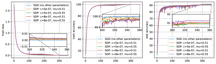
Figure 3: Performance comparison results of AltSDP (SDP) and SGD under different hyperparameters on VGG-16, CIFAR-10 task. Left: training loss. Center: training accuracy. Right: testing accuracy.

We compare AltSDP with different methods that have published results in terms of the test accuracy and Floating-point Operations (FLOPs) reduction. Some methods are reproduced by [23] and obtain better performance than the originally published ones, then we use the better results in our comparisons with appending a label “(New)”. The base ResNet model is implemented following [2, 23] and the base VGG model is implemented following [16, 23]. The detailed parameters for training are list in Appendix. For each method, we present its baseline model accuracy, pruned model accuracy, the accuracy drop between baseline and pruned model, and FLOPs reduction after pruning. A negative accuracy drop indicates that the pruned model performances better than its unpruned baseline model. Specifically, the pruned model accuracy reported for our AltSDP is without fine-tune or retraining. More experiments on the WRN28$\times$10 network and MNIST datasets can be found in the Appendix.

4.2 Performance Comparison Results

Table 1 shows the performance of different methods on CIFAR datasets, which is the most widely used dataset for pruning task. On CIFAR-10, ResNet-56 task, our method obtains the smallest accuracy drop (-0.10%) and the best pruned accuracy (93.90%) with highest FLOPs reduction (55%). On CIFAR-10, VGG-16 task, our method also obtains the smallest accuracy drop (-0.09%) and the best pruned accuracy (93.97%) with highest FLOPs reduction (55%). Since few structured pruning results on CIFAR-100 dataset are reported in previous works, we only compared with three different algorithms. And as shown in Table 1, our method still achieves the smallest accuracy drop (-0.06 for ResNet-56 and -0.46 for VGG-16) and the best pruned accuracy (72.55 for ResNet-56 and 74.29 for VGG-16) under similar FLOPs reduction.

Table 2 shows the performance of different methods on large FLOPs reduction. Since there exist little related works on structured pruning with large FLOPs reduction, the comparison results are mainly from [7]. Specifically, 400 total epochs are used to training and fine-tune/retraining for other methods reproduced in [7], while we only train 200+ epochs for AltSDP without retraining. Our method achieves the smallest accuracy drop (0.86%) and the best pruned accuracy (92.94%) with highest FLOPs reduction (72%).

4.3 Analysis

In this Section, we first empirically study the effect of hyper-parameters in AltSDP. Then, we train a basic DNN on MNIST, VGG-Net on CIFAR-10 and WRAN20$\times$10 on CIFAR-100 to checking whether AltSDP performs structured directional pruning and reaches the same flat minimum valley obtained by SGD. Similar analysis strategy has been done by [7, 39, 40, 41, 42] and the base VGG model and method for visualizing are implemented following [39, 7].

We then displays the performance of SGD and AltSDP with different hyper-parameter $c$ and $\mu$ on VGG-16, CIFAR-10 task. As shown in Figure 3, the training loss of AltSDP is almost the same with SGD (diff. less than 0.003 in Table 3) when pruning, which implies that AltSDP reaches the same flat minimum valley found by SGD. And the test accuracy of AltSDP is similar with SGD. Table 3 shows more details of Figure 3, where sparsity denotes the non-zero parameter ratio after training. We find that AltSDP performs worse than SGD when $\mu=0.40$, but performs better than SGD under other parameter settings. This is reasonable according to Theorem 2, which suggests that $\mu$ should be slightly greater than 0.5. Moreover, as hyperparameters $c$ and $\mu$ become larger, AltSDP pushes more parameters to zero and the sparsity becomes larger.

Finally, we check whether AltSDP reaches the same valley found by SGD. We train VGG16 on CIFAR-10 until nearly zero training loss using both SGD and AltSDP. We use the method of [43] to search for a quadratic Bézier curve of minimal training loss connecting the minima found by optimizers. We can see that AltSDP performs the structured directional pruning since the learned parameters of both SGD and AltSDP lie in the same flat minimum valley on the training loss landscape if $\mu$ and $c$ is properly tuned, namely $\mu=0.51$ and $c=5\times 10^{-7}$.

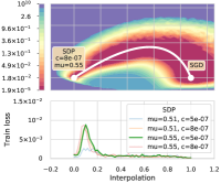
(a)

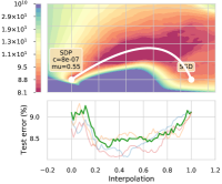
(b)

Figure 4: The upper figures show the contour of training loss and testing error on the hyperplane. Left: Train loss on CIFAR-10 and VGG16 task. Right: Test error on CIFAR-10 and VGG16 task. The lower figures show the corresponding white curve (Bézier curve), which contains the interpolating minimizers of SGD and AltSDP under different $\mu$.

5 Conclusions

In this paper we propose the structured directional pruning method to compress deep neural networks while preserving accuracy, which is based on orthogonal projecting the sparse perturbations onto the flat minimum valley found by optimizers. A fast solver AltSDP is also proposed to achieve structured directional pruning. Theoretically, we prove that AltSDP achieves directional pruning after sufficient training. Experimentally, we demonstrate the benefits of structured directional pruning and show that it achieves the state-of-the-art result. Experiments using VGG-Net and ResNet on CIFAR-10 and CIFAR-100 datasets show that our method obtains the best pruned accuracy (i.e. 93.97% on VGG16, CIFAR-10 task) without retraining. Moreover, experiments using DNN, VGG-Net and WRN28$\times$10 on MNIST, CIFAR-10 and CIFAR-100 datasets demonstrate our method performs directional pruning, reaching the same minimal valley as the optimizer.

Appendix A Proof of Main Theorems

A.1 Proof of Theorem 1

Theorem 1. Consider the optimization problem

$$\arg\min_{{\bm{w}}_{i}}\left\{\frac{1}{2}\|{\bm{w}}_{i}^{\star}-{\bm{w}}_{i}\|_{2}^{2}+\lambda{s}_{i}\|{\bm{w}}_{i}\|_{2}\right\}.$$ (14)

For ${\bm{w}}_{i}^{\star}\in\mathbb{R}^{d}\backslash\{\bm{0}\},{s}_{i}\in\mathbb{R},\lambda>0$, (14) has an explicit solution:

$$\hat{\bm{w}}_{i}=\left(1-\frac{\lambda{s}_{i}}{\|{\bm{w}}_{i}^{\star}\|_{2}}\right)_{+}{\bm{w}}_{i}^{\star}.$$ (15)

Proof.

Let’s $\hat{\bm{w}}_{i}$ denotes the solution for (14), we prove $\hat{\bm{w}}_{i}$ follows the formulation in (15) from three perspectives: ${s}_{i}=0,{s}_{i}>0$ and ${s}_{i}<0$. Set $f({\bm{w}}_{i}):=\frac{1}{2}\|{\bm{w}}_{i}^{\star}-{\bm{w}}_{i}\|_{2}^{2}+\lambda{s}_{i}\|{\bm{w}}_{i}\|_{2}$. First, when ${s}_{i}=0$, the solution $\hat{\bm{w}}_{i}={\bm{w}}_{i}^{\star}$. Then, on the one hand, when ${s}_{i}>0$, the objective function is convex, therefore $\nabla f(\hat{\bm{w}}_{i})=0$. We have

$$\nabla f(\hat{\bm{w}}_{i})=\hat{\bm{w}}_{i}-{\bm{w}}_{i}^{\star}+\frac{\lambda{s}_{i}\hat{\bm{w}}_{i}}{\|\hat{\bm{w}}_{i}\|_{2}}=0,$$ (16)

which yields ${\bm{w}}_{i}^{\star}=\left(1+\lambda{s}_{i}/\|\hat{\bm{w}}_{i}\|_{2}\right)\hat{\bm{w}}_{i}$. Since $1+\lambda{s}_{i}/\|\hat{\bm{w}}_{i}\|_{2}>0$ is a scalar, we have ${\bm{w}}_{i}^{\star}$ and $\hat{\bm{w}}_{i}$ in the same direction, hence

$$\frac{\hat{\bm{w}}_{i}}{\|\hat{\bm{w}}_{i}\|_{2}}=\frac{{\bm{w}}_{i}^{\star}}{\|{\bm{w}}_{i}^{\star}\|_{2}}.$$ (17)

By substituting (17) into (16), we finish the proof for ${s}_{i}>0$.

On the other hand, when ${s}_{i}<0$, the objective function is not convex, therefore we need to check the value of $f({\bm{w}}_{i})$ at stationary points. If ${\bm{w}}_{i}^{\star}=0$, then $\hat{\bm{w}}_{i}=0$ is the solution for (14). If ${\bm{w}}_{i}^{\star}\neq 0$, we have

• On $\|{\bm{w}}_{i}\|_{2}=-\lambda s_{i}$, $\nabla f({\bm{w}}_{i})=-{\bm{w}}_{i}^{\star}\neq 0$, there is no stationary point.

• On $\|{\bm{w}}_{i}\|_{2}>-\lambda s_{i}$, we have $(1+\lambda s_{i}/\|{\bm{w}}_{i}\|_{2})>0$. The stationary point ${\bm{w}}_{sp1}$ is $(1-\lambda s_{i}/\|{\bm{w}}_{i}^{\star}\|_{2}){\bm{w}}_{i}^{\star}$ with objective function value $f({\bm{w}}_{sp1})$

  $$f({\bm{w}}_{sp1})=\frac{1}{2}\left\|\frac{\lambda s_{i}{\bm{w}}_{i}^{\star}}{\|{\bm{w}}_{i}^{\star}\|_{2}}\right\|_{2}^{2}+\lambda s_{i}\left\|(1-\frac{\lambda s_{i}}{\|{\bm{w}}_{i}^{\star}\|_{2}}){\bm{w}}_{i}^{\star}\right\|_{2}.$$

• On $\|{\bm{w}}_{i}\|_{2}<-\lambda s_{i}$, we have $(1+\lambda s_{i}/\|{\bm{w}}_{i}\|_{2})<0$. The stationary point ${\bm{w}}_{sp1}$ is $(1+\lambda s_{i}/\|{\bm{w}}_{i}^{\star}\|_{2}){\bm{w}}_{i}^{\star}$ with objective function value $f({\bm{w}}_{sp2})$

  $$f({\bm{w}}_{sp2}) =\frac{1}{2}\left\|\frac{\lambda s_{i}{\bm{w}}_{i}^{\star}}{\|{\bm{w}}_{i}^{\star}\|_{2}}\right\|_{2}^{2}+\lambda s_{i}\left\|(1+\frac{\lambda s_{i}}{\|{\bm{w}}_{i}^{\star}\|_{2}}){\bm{w}}_{i}^{\star}\right\|_{2}.$$

  Since $\lambda s_{i}<0$ and ${\bm{w}}_{i}^{\star}\neq 0$, we have

  $$\left\|(1-\frac{\lambda s_{i}}{\|{\bm{w}}_{i}^{\star}\|_{2}}){\bm{w}}_{i}^{\star}\right\|_{2}>\left\|(1+\frac{\lambda s_{i}}{\|{\bm{w}}_{i}^{\star}\|_{2}}){\bm{w}}_{i}^{\star}\right\|_{2}.$$

  Then $f({\bm{w}}_{sp1})<f({\bm{w}}_{sp2})$, which means the global minimizer of $f({\bm{w}}_{i})$ is the stationary point $(1-\lambda s_{i}){\bm{w}}_{i}^{\star}/\|{\bm{w}}_{i}^{\star}\|_{2}$ on $\|{\bm{w}}_{i}\|_{2}>-\lambda s_{i}$. We finish the proof for ${s}_{i}>0$.

Then we complete the proof of Theorem 1. ∎

A.2 Proof of Theorem 2

Theorem 2. Under Assumptions 1-6, suppose $\mu\in(0.5,1)$ and $c>0$, when $\gamma\rightarrow 0$, AltSDP achieves structured directional pruning based on ${\bm{w}}^{SGD}(t)$ asymptotically, i.e., we have for $t>\bar{T}$

$${\bm{w}}_{\gamma}(t)\overset{d}{\approx}\arg\min_{{\bm{w}}\in\mathbb{R}^{d}}\frac{1}{2}\|{\bm{w}}^{SGD}(t)-{\bm{w}}\|_{2}^{2}+\lambda_{\gamma,t}\sum_{i=1}^{|\mathcal{G}|}\bar{s}_{i}\|{\bm{w}}_{i}\|_{2},$$ (18)

and

$${\bm{w}}_{\gamma,i}(t)\overset{d}{\approx}\left(1-\frac{\lambda_{\gamma,t}\bar{s}_{i}}{\|{\bm{w}}_{i}^{SGD}(t)\|_{2}}\right)_{+}{\bm{w}}_{i}^{SGD}(t),~{}i=1,...,|\mathcal{G}|,$$ (19)

where $\lambda_{\gamma,t}=c\sqrt{\gamma}t^{\mu}$; $\overset{d}{\approx}$ represents “asymptotic in distribution” under the empirical probability measure of gradients; and $\bar{s}_{i}$ satisfies $\lim_{t\rightarrow\infty}|\bar{s}_{i}-s_{i}|=0$ for all $i$.

To proof Theorem 2, we first present the following useful Theorem 3, which is proved in Appendix A.3.

Theorem 3.

Suppose (A1), (A2) and (A3) hold, and assume that the root of the coordinates in ${\bm{w}}(t)$ occur at time $\{T_{k}\}_{k=1}^{\infty}\subset[0,\infty)$. Let ${\bm{w}}_{0}$ with ${w}_{0,j}\neq 0$ (e.g. from a normal distribution) and $T_{0}=0$. Then, as $\gamma$ is small, for $t\in(T_{K},T_{K+1})$,

$${\bm{v}}_{\gamma}(t) \overset{d}{\approx}{\bm{w}}(t)+\sqrt{\gamma}ct^{\mu}E_{\mathcal{G}}({\bm{w}}(t))-\sqrt{\gamma}c\sum_{k=1}^{K}\Big{\{}\Phi(t,T_{k})\left\{E_{\mathcal{G}}({\bm{w}}(T_{k}^{+}))-E_{\mathcal{G}}({\bm{w}}(T_{k}^{-}))\right\}T_{k}^{\mu}\Big{\}}$$

$$~{}~{}~{}~{}~{}-\sqrt{\gamma}{c\int_{0}^{t}\Phi(t,s)\frac{\partial E_{\mathcal{G}}({\bm{w}}(s))s^{\mu}}{\partial s}ds}+\sqrt{\gamma}\int_{0}^{t}\Phi(t,s){\Sigma}^{1/2}({\bm{w}}(s))d{\bm{B}}(s)$$ (20)

where $\overset{d}{\approx}$ denotes approximately in distribution, ${\bm{B}}(s)$ is a $d$-dimensional standard Brownian motion, $\Phi(t,s)\in\mathbb{R}^{d\times d}$ is the principal matrix solution of the matrix ODE system,

$$d{\bm{x}}(t)=-H({\bm{w}}(t)){\bm{x}}(t)dt,\quad{\bm{x}}(t_{0})={\bm{x}}_{0},$$ (21)

and $\Sigma({\bm{w}})$ is defined as

$$\Sigma({\bm{w}}):=\mathbb{E}_{Z}\left[(\nabla f({\bm{w}};Z)-G({\bm{w}})(\nabla f({\bm{w}};Z)-G({\bm{w}})^{T}\right].$$

Theorem 3 presents the distribution dynamics of $\bm{v}_{\gamma}(t)$ in (AltSDP-(a)) with ${\bm{v}}_{\gamma}(t):={\bm{v}}_{\left\lfloor t/\gamma\right\rfloor}$. Next, we start prove Theorem 2, which equals to prove the distribution dynamics of $\bm{w}_{\gamma,i}(t)$ in (AltSDP-(b)) approximately in distribution with $\left(1-\frac{\lambda_{\gamma,t}\bar{s}_{i}}{\|{\bm{w}}_{i}^{SGD}\|_{2}}\right){\bm{w}}_{i}^{SGD}$.

Proof.

To start with, recall that

$${\bm{v}}_{n+1} ={\bm{v}}_{n}-\gamma\nabla f({\bm{w}}_{n};{Z}_{n+1})$$ (AltSDP-(a))

$${\bm{w}}_{n+1} =\arg\min_{{\bm{w}}\in\mathbb{R}^{d}}\{\frac{1}{2}\|{\bm{w}}\|_{2}^{2}-{\bm{w}}^{T}{\bm{v}}_{n+1}+g(n,\gamma)\sum_{i=1}^{|\mathcal{G}|}\|{\bm{w}}_{i}\|_{2}\}.$$ (AltSDP-(b))

To analysis the distribution dynamics of $\bm{w}_{\gamma,i}(t)$, we first define

$$\zeta_{\gamma,i}({\bm{w}}_{\gamma,i}(t)):=\frac{1}{2}\|{\bm{w}}_{\gamma,i}(t)\|_{2}^{2}+\sqrt{\gamma}ct^{\mu}\|{\bm{w}}_{\gamma,i}(t)\|_{2}.$$ (22)

Then we have its Fenchel conjugate is given by [27]

$$\zeta_{\gamma,i}^{*}({\bm{v}}_{\gamma,i}(t))=\max_{{\bm{w}}_{\gamma,i}(t)}\left\{{\bm{w}}_{\gamma,i}(t)^{T}{\bm{v}}_{\gamma,i}(t)-\frac{1}{2}\|{\bm{w}}_{\gamma,i}(t)\|_{2}^{2}-\sqrt{\gamma}ct^{\mu}\|{\bm{w}}_{\gamma,i}(t)\|_{2}\right\},$$

and the derivative of its Fenchel conjugate is given by [27]

$$\nabla\zeta_{\gamma,i}^{*}({\bm{v}}_{\gamma,i}(t)):=\arg\min_{{\bm{w}}_{\gamma,i}(t)}\left\{\frac{1}{2}\|{\bm{w}}_{\gamma,i}(t)\|_{2}^{2}+\sqrt{\gamma}ct^{\mu}\|{\bm{w}}_{\gamma,i}(t)\|_{2}-{\bm{w}}_{\gamma,i}(t)^{T}{\bm{v}}_{\gamma,i}(t)\right\}.$$ (23)

Hence, by noting that (23) is a convex function, let the gradient equals to zero we have

$${\bm{w}}_{\gamma,i}(t)+\sqrt{\gamma}ct^{\mu}{\bm{w}}_{\gamma,i}(t)/\|{\bm{w}}_{\gamma,i}(t)\|_{2}-{\bm{v}}_{\gamma,i}(t)=0,$$ (24)

which yields ${\bm{v}}_{\gamma,i}(t)=\left(1+\sqrt{\gamma}ct^{\mu}/\|{\bm{w}}_{\gamma,i}(t)\|_{2}\right){\bm{w}}_{\gamma,i}(t)$. Since $(1+\sqrt{\gamma}ct^{\mu}/\|{\bm{w}}_{\gamma,i}(t)\|_{2})>0$ is a scalar, we have ${\bm{v}}_{\gamma,i}(t)$ and ${\bm{w}}_{\gamma,i}(t)$ in the same direction, hence

$$\frac{{\bm{v}}_{\gamma,i}(t)}{\|{\bm{v}}_{\gamma,i}(t)\|_{2}}=\frac{{\bm{w}}_{\gamma,i}(t)}{\|{\bm{w}}_{\gamma,i}(t)\|_{2}}.$$ (25)

By substituting (25) into (24), we have

$${\bm{w}}_{\gamma,i}(t)=\nabla\zeta_{\gamma,i}^{*}({\bm{v}}_{\gamma,i}(t))={\bm{v}}_{\gamma,i}(t)-\sqrt{\gamma}ct^{\mu}E({\bm{v}}_{\gamma,i}(t)).$$ (26)

Now, we obtain the relationshop between ${\bm{w}}_{\gamma,i}(t)$ and ${\bm{v}}_{\gamma,i}(t)$ in (26). Next, we prove (26) approximately in distribution with $\left(1-\frac{\lambda_{\gamma,t}\bar{s}_{i}}{\|{\bm{w}}_{i}^{SGD}\|_{2}}\right){\bm{w}}_{i}^{SGD}$ based on Theorem 3. Follows by (20) in Theorem 3 we have

$${\bm{v}}_{\gamma}(t) \overset{d}{\approx}{\bm{w}}(t)+\sqrt{\gamma}ct^{\mu}E_{\mathcal{G}}({\bm{w}}(t))-\sqrt{\gamma}c\sum_{k=1}^{K}\Big{\{}\Phi(t,T_{k})\left\{E_{\mathcal{G}}({\bm{w}}(T_{k}^{+}))-E_{\mathcal{G}}({\bm{w}}(T_{k}^{-}))\right\}T_{k}^{\mu}\Big{\}}$$

$$~{}~{}~{}~{}~{}-\sqrt{\gamma}{c\int_{0}^{t}\Phi(t,s)\frac{\partial E_{\mathcal{G}}({\bm{w}}(s))s^{\mu}}{\partial s}ds}+\sqrt{\gamma}\int_{0}^{t}\Phi(t,s){\Sigma}^{1/2}({\bm{w}}(s))d{\bm{B}}(s)$$

$$={\bm{w}}(t)+\sqrt{\gamma}ct^{\mu}E_{\mathcal{G}}({\bm{w}}(t))-\sqrt{\gamma}{\bm{\delta}(t)}+\sqrt{\gamma}{\bm{U}}(t),$$ (27)

where ${\bm{\delta}}(t)={\bm{\delta}}_{1}(t)+{\bm{\delta}}_{2}(t)$ and ${\bm{U}}(t)$ are given by

$${\bm{\delta}}_{1}(t):=c\sum_{k=1}^{K}\Big{\{}\Phi(t,T_{k})\left\{E_{\mathcal{G}}({\bm{w}}(T_{k}^{+}))-E_{\mathcal{G}}({\bm{w}}(T_{k}^{-}))\right\}T_{k}^{\mu}\Big{\}},$$

$${\bm{\delta}}_{2}(t):=c\int_{0}^{t}\Phi(t,s)\frac{\partial E_{\mathcal{G}}({\bm{w}}(s))s^{\mu}}{\partial s}ds,$$

$${\bm{U}}(t):=\int_{0}^{t}\Phi(t,s){\Sigma}^{1/2}({\bm{w}}(s))d{\bm{B}}(s).$$

By substituting (27) into (26), for each $i$ we have

$${\bm{w}}_{\gamma,i}(t) \overset{d}{\approx}{\bm{w}}_{i}(t)+\sqrt{\gamma}{\bm{U}}_{i}(t)-\sqrt{\gamma}{\bm{\delta}}_{i}(t)+\sqrt{\gamma}ct^{\mu}\left(E({\bm{w}}_{\gamma,i}(t))-E({\bm{v}}_{\gamma,i}(t))\right),$$

$$={\bm{w}}_{i}(t)+\sqrt{\gamma}{\bm{U}}_{i}(t)-\sqrt{\gamma}{\bm{\delta}}_{i}(t),$$ (28)

where the equality follows by (25). Following the analysis in [6, 44], the piecewise constant process of SGD follows

$$w_{j}^{SGD}(t)\overset{d}{\approx}w_{j}(t)+\sqrt{\gamma}{\bm{U}}_{j}(t),~{}j={1,2,\cdots,d},$$

yields

$${\bm{w}}_{i}^{SGD}\overset{d}{\approx}{\bm{w}}_{i}(t)+\sqrt{\gamma}{\bm{U}}_{i}(t),~{}i=1,2,...,|\mathcal{G}|.$$

Then we have

$${\bm{w}}_{\gamma,i}(t)\overset{d}{\approx}{\bm{w}}_{i}^{SGD}(t)-\sqrt{\gamma}{\bm{\delta}}_{i}(t),~{}i=1,2,...,|\mathcal{G}|.$$ (29)

We next prove for $t\rightarrow\infty$,

$${\bm{\delta}}(t)=ct^{\mu}{\Pi}E_{\mathcal{G}}({\bm{w}}(t))+o(t^{\mu})+O(t^{\mu-1}).$$

To obtain this, we need to find the principal matrix solution $\Phi(t,s)$ in ${\bm{\delta}}_{i}(t)$. Recall (12) that

$$\frac{d\Phi(t,s)}{dt}=-H({\bm{w}}(t))\Phi(t,s),\quad\Phi(s,s)=I_{d}.$$

Following the Levinson theorem [45], when $a_{t}\rightarrow 0$, there exists a real symmetric matrix ${\bar{H}}=P\Lambda P^{T}$ satisfying

$$\int_{t}^{\infty}\|H({\bm{w}}(s))-{\bar{H}}\|ds=O(a_{t}),$$

where $\Lambda={\rm diag}(\lambda_{1},\cdots,\lambda_{d})$ is a diagonal matrix with non-negative values and $P$ is an orhonormal matrix with its column vectors are eigenvectors $\bm{u}_{j}$. Following the proof in [7] and Levinson theorem in [45], we get the principal matrix solution $\Phi(t,s)$ in (21) satisfies

$$\Phi(\tau,s)=P(I_{d}+O(a_{\tau}))e^{-\Lambda(\tau-s)}P^{T}=P_{0}P_{0}^{T}+O(e^{-\underline{\lambda}(\tau-s)})+O(a_{\tau}),$$ (30)

where $\underline{\lambda}$ is the least positive eigenvalue of ${\bar{H}}$, the column vectors of $P_{0}$ are eigenvectors associated with the zero eigenvalue, i.e., $P_{0}P_{0}^{T}=\sum_{j:\bar{H}\bm{u}_{j}=0}\bm{u}_{j}\bm{u}_{j}^{T}$. Then we have

$${\bm{\delta}}_{1}(t) =c\sum_{k=1}^{K}\Big{\{}\Phi(t,T_{k})\left\{E_{\mathcal{G}}({\bm{w}}(T_{k}^{+}))-E_{\mathcal{G}}({\bm{w}}(T_{k}^{-}))\right\}T_{k}^{\mu}\Big{\}}$$

$$=cP_{0}P_{0}^{T}\sum_{k=1}^{K}\Big{\{}\left\{E_{\mathcal{G}}({\bm{w}}(T_{k}^{+}))-E_{\mathcal{G}}({\bm{w}}(T_{k}^{-}))\right\}T_{k}^{\mu}\Big{\}}+O(e^{-\underline{\lambda}(t-T_{K})}T_{k}^{\mu})+O(a_{t}T_{k}^{\mu}),$$ (31)

where the first term of $\delta_{1}(t)$ can be rewritten as

$$~{}~{}~{}~{}~{}cP_{0}P_{0}^{T}\sum_{k=1}^{K}\Big{\{}\left\{E_{\mathcal{G}}({\bm{w}}(T_{k}^{+}))-E_{\mathcal{G}}({\bm{w}}(T_{k}^{-}))\right\}T_{k}^{\mu}\Big{\}}$$

$$=cP_{0}P_{0}^{T}\left\{E_{\mathcal{G}}({\bm{w}}(T_{K})^{+})T_{K}^{\mu}-\sum_{k=1}^{K}\left\{E_{\mathcal{G}}({\bm{w}}(T_{k}^{-}))T_{k}^{\mu}-E_{\mathcal{G}}({\bm{w}}(T_{k-1}^{+}))T_{k-1}^{\mu}\right\}\right\}$$

$$=cP_{0}P_{0}^{T}\left\{E_{\mathcal{G}}({\bm{w}}(T_{K}^{+}))T_{K}^{\mu}-E_{\mathcal{G}}({\bm{w}}(t))t^{\mu}\big{|}_{T_{K-1}}^{T_{K}}-\cdots-E_{\mathcal{G}}({\bm{w}}(t))t^{\mu}\big{|}_{T_{0}}^{T_{1}}\right\}$$

$$=cP_{0}P_{0}^{T}\left\{E_{\mathcal{G}}({\bm{w}}(T_{K}^{+}))T_{K}^{\mu}-\int_{T_{K-1}}^{T_{K}}\frac{\partial E_{\mathcal{G}}({\bm{w}}(s))s^{\mu}}{\partial s}ds-\cdots-\int_{0}^{T_{1}}\frac{\partial E_{\mathcal{G}}({\bm{w}}(s))s^{\mu}}{\partial s}ds\right\}$$

$$=cP_{0}P_{0}^{T}\left\{E_{\mathcal{G}}({\bm{w}}(T_{K}^{+}))T_{K}^{\mu}-\int_{0}^{T_{K}}\frac{\partial E_{\mathcal{G}}({\bm{w}}(s))s^{\mu}}{\partial s}ds\right\}.$$ (32)

Combining (A.2) and (A.2), we get

$${\bm{\delta}}_{1}(t)=cP_{0}P_{0}^{T}\left\{E_{\mathcal{G}}({\bm{w}}(T_{K}^{+}))T_{K}^{\mu}-\int_{0}^{T_{K}}\frac{\partial E_{\mathcal{G}}({\bm{w}}(s))s^{\mu}}{\partial s}ds\right\}+O(e^{-\underline{\lambda}(t-T_{K})}T_{k}^{\mu})+O(a_{t}T_{k}^{\mu}).$$

Then by substituting (30) into $\bm{\delta}_{2}(t)$, we next obtain

$${\bm{\delta}}_{2}(t) =c\int_{0}^{t}\Phi(t,s)\frac{\partial E_{\mathcal{G}}({\bm{w}}(s))s^{\mu}}{\partial s}ds$$

$$=cP_{0}P_{0}^{T}\int_{0}^{t}\frac{\partial E_{\mathcal{G}}({\bm{w}}(s))s^{\mu}}{\partial s}ds+O\left(c\int_{0}^{t}e^{-\underline{\lambda}(t-s)}\frac{\partial E_{\mathcal{G}}({\bm{w}}(s))s^{\mu}}{\partial s}ds\right)$$

$$~{}~{}~{}~{}~{}~{}~{}~{}~{}~{}~{}~{}~{}~{}~{}~{}~{}~{}~{}~{}~{}~{}~{}~{}~{}~{}~{}~{}~{}~{}~{}~{}~{}~{}~{}~{}~{}~{}~{}~{}~{}~{}~{}~{}~{}~{}~{}~{}~{}~{}~{}~{}~{}~{}~{}~{}+O\left(c\int_{0}^{t}a_{t}\frac{\partial E_{\mathcal{G}}({\bm{w}}(s))s^{\mu}}{\partial s}ds\right)$$ (33)

where $\left\|E_{\mathcal{G}}({\bm{w}}(s))\right\|=|\mathcal{G}|^{1/2}$. Then we have

$$O\left(c\int_{0}^{t}e^{-\underline{\lambda}(t-s)}\frac{\partial E_{\mathcal{G}}({\bm{w}}(s))s^{\mu}}{\partial s}ds\right) \lesssim c\int_{0}^{t}e^{-\underline{\lambda}(t-s)}\frac{\left\|\partial E_{\mathcal{G}}({\bm{w}}(s))\right\|s^{\mu}}{\partial s}ds$$

$$=c|\mathcal{G}|^{1/2}\int_{0}^{t}e^{-\underline{\lambda}(t-s)}\frac{\partial s^{\mu}}{\partial s}ds$$

$$\leq c\mu d^{1/2}\int_{0}^{t}s^{\mu-1}e^{-\underline{\lambda}(t-s)}ds\overset{(a)}{=}O(t^{\mu-1})$$ (34)

and

$$O\left(c\int_{0}^{t}a_{t}\frac{\partial E_{\mathcal{G}}({\bm{w}}(s))s^{\mu}}{\partial s}ds\right)\lesssim c\mu|\mathcal{G}|^{1/2}\int_{0}^{t}s^{\mu-1}a_{t}ds=O(a_{t}t^{\mu})$$ (35)

where $(a)$ follows by using the similar arguments as the proof of Theorem 4.2 in [27] with $\mu\in(0.5,1)$. Combining (A.2), (34) and (35) we get

$${\bm{\delta}}_{2}(t)=cP_{0}P_{0}^{T}\int_{0}^{t}\frac{\partial E_{\mathcal{G}}({\bm{w}}(s))s^{\mu}}{\partial s}ds+O(t^{\mu-1})+O(a_{t}t^{\mu}).$$

Note that $a_{t}t^{\mu}>a_{t}T_{K}^{\mu}$ for $\mu>0,t>T_{K}$ and $e^{-\underline{\lambda}(t-T_{K})}\rightarrow 0$. Then

$${\bm{\delta}}(t) ={\bm{\delta}}_{1}(t)+{\bm{\delta}}_{2}(t)$$

$$=cP_{0}P_{0}^{T}\left\{E_{\mathcal{G}}({\bm{w}}(T_{K}^{+}))T_{K}^{\mu}-\int_{0}^{T_{K}}\frac{\partial E_{\mathcal{G}}({\bm{w}}(s))s^{\mu}}{\partial s}ds+\int_{0}^{t}\frac{\partial E_{\mathcal{G}}({\bm{w}}(s))s^{\mu}}{\partial s}ds\right\}$$

$$~{}~{}~{}~{}~{}~{}~{}~{}+O(t^{\mu-1})+O(a_{t}t^{\mu})$$

$$=cP_{0}P_{0}^{T}\left\{E_{\mathcal{G}}({\bm{w}}(T_{K}^{+}))T_{K}^{\mu}+\int_{T_{K}}^{t}\frac{\partial E_{\mathcal{G}}({\bm{w}}(s))s^{\mu}}{\partial s}ds\right\}+O(t^{\mu-1})+O(a_{t}t^{\mu})$$

$$=cP_{0}P_{0}^{T}\left\{E_{\mathcal{G}}({\bm{w}}(T_{K}^{+}))T_{K}^{\mu}+E_{\mathcal{G}}({\bm{w}}(s))s^{\mu}\big{|}_{T_{K}}^{t}\right\}+O(t^{\mu-1})+O(a_{t}t^{\mu})$$

$$=cP_{0}P_{0}^{T}E_{\mathcal{G}}({\bm{w}}(t))t^{\mu}+O(t^{\mu-1})+O(a_{t}t^{\mu})$$

$$\overset{(a)}{=}c{\Pi}E_{\mathcal{G}}({\bm{w}}(t))t^{\mu}+O(t^{\mu-1})+o(t^{\mu}),$$

where ${\Pi}=P_{0}P_{0}^{T}$ and $(a)$ is due to

$$\lim_{t\rightarrow 0}\frac{a_{t}t^{\mu}}{t^{\mu}}=\lim_{t\rightarrow 0}a_{t}=0.$$

Then set ${s_{i}}=E({\bm{w}}(t))\cdot\left\{{\Pi}E_{\mathcal{G}}({\bm{w}}(t))\right\}_{i}$, we get

$${\bm{\delta}}_{i}(t)=ct^{\mu}s_{i}E({\bm{w}}_{i}(t))+o(t^{\mu})+O(t^{\mu-1}).$$ (36)

To this end, by substituting (36) into (29), we have

$${\bm{w}}_{\gamma,i}(t) \overset{d}{\approx}{\bm{w}}_{i}^{SGD}(t)-\sqrt{\gamma}\left(ct^{\mu}s_{i}E({\bm{w}}_{i}(t))+o(t^{\mu})+O(t^{\mu-1})\right),~{}i=1,2,...,|\mathcal{G}|$$

$$={\bm{w}}_{i}^{SGD}(t)-\sqrt{\gamma}ct^{\mu}\bar{s}_{i}E({\bm{w}}_{i}(t)),~{}i=1,2,...,|\mathcal{G}|,$$

where $\bar{s}_{i}=s_{i}+\frac{o(t^{\mu})}{c\sqrt{\gamma}t^{\mu}}+\frac{O(t^{\mu-1})}{c\sqrt{\gamma}t^{\mu}}$ and hence $\lim_{t\rightarrow\infty}|\bar{s}_{i}-s_{i}|=0$. Based on Assumption 6 we can further have

$${\bm{w}}_{\gamma,i}(t)\overset{d}{\approx}{\bm{w}}_{i}^{SGD}(t)-c\sqrt{\gamma}t^{\mu}\bar{s}_{i}E({\bm{w}}_{i}^{SGD}(t)),~{}i=1,2,...,|\mathcal{G}|,$$

hence we obtain (19). Based on Theorem 1, we further obtain (18). Then we complete the proof. ∎

A.3 Proof of Theorem 3

Proof.

To prove

$${\bm{v}}_{\gamma}(t) \overset{d}{\approx}{\bm{w}}(t)+\sqrt{\gamma}ct^{\mu}E_{\mathcal{G}}({\bm{w}}(t))-\sqrt{\gamma}c\sum_{k=1}^{K}\Big{\{}\Phi(t,T_{k})\left\{E_{\mathcal{G}}({\bm{w}}(T_{k}^{+}))-E_{\mathcal{G}}({\bm{w}}(T_{k}^{-}))\right\}T_{k}^{\mu}\Big{\}}$$

$$~{}~{}~{}~{}~{}-\sqrt{\gamma}{c\int_{0}^{t}\Phi(t,s)\frac{\partial E_{\mathcal{G}}({\bm{w}}(s))s^{\mu}}{\partial s}ds}+\sqrt{\gamma}\int_{0}^{t}\Phi(t,s){\Sigma}^{1/2}({\bm{w}}(s))d{\bm{B}}(s),$$

we define the centered and scaled processes

$${\bm{V}}_{\gamma}(t):=\frac{{\bm{v}}_{\gamma}(t)-{\bm{w}}(t)}{\sqrt{\gamma}},$$ (37)

then we need to prove

$${\bm{V}}_{\gamma}(t) \overset{d}{\approx}ct^{\mu}E_{\mathcal{G}}({\bm{w}}(t))-c\sum_{k=1}^{K}\Big{\{}\Phi(t,T_{k})\left\{E_{\mathcal{G}}({\bm{w}}(T_{k}^{+}))-E_{\mathcal{G}}({\bm{w}}(T_{k}^{-}))\right\}T_{k}^{\mu}\Big{\}}$$

$$~{}~{}~{}~{}~{}-c\int_{0}^{t}\Phi(t,s)\frac{\partial E_{\mathcal{G}}({\bm{w}}(s))s^{\mu}}{\partial s}ds+\int_{0}^{t}\Phi(t,s){\Sigma}^{1/2}({\bm{w}}(s))d{\bm{B}}(s).$$

By Theorem 3.13 in [27], ${\bm{V}}_{\gamma}\overset{d}{\approx}{\bm{V}}$ on $(T_{k},T_{k+1})$ for each $k=0,\dots,K$ as $\gamma$ is small, where $V$ obeys the stochastic differential equation (SDE):

$$d{\bm{V}}(t)=-H({\bm{w}}(t))\nabla\tilde{\zeta}^{*}(\bm{V}(t))dt+{\Sigma}^{1/2}({\bm{w}}(t))d{\bm{B}}(t),$$ (38)

where the initial ${\bm{V}}(T_{k})={\bm{V}}(T_{k}^{-})$, ${\bm{B}}(t)$ is the $d$-dimensional standard Brownian motion, and $\tilde{\zeta}^{*}(\bm{V}(t))$ is the Fenchel conjugate of $\tilde{\zeta}({\bm{W}}(t))$. The function $\tilde{\zeta}(\cdot)$ is defined as $\tilde{\zeta}({\bm{w}}(t)):=\lim_{\gamma\rightarrow 0}\tilde{\zeta}_{\gamma}(\bm{w}(t))$ with $\tilde{\zeta}_{\gamma}(\bm{w}(t))$ being the local Bregman divergence of ${\zeta}_{\gamma}(\bm{w}(t))$ in (22) at $(\bm{v}(t),\bm{w}(t))$. In particular, we have

$$\tilde{\zeta}_{\gamma}(\bm{u}(t)) :={\gamma}^{-1}\bigg{(}{\zeta}_{\gamma}({\bm{w}}(t)+\sqrt{\gamma}{\bm{u}}(t))-{\zeta}_{\gamma}({\bm{w}}(t))-\left\langle\sqrt{\gamma}{\bm{u}}(t),{\bm{w}}(t)\right\rangle\bigg{)}$$

$$={\gamma}^{-1}\bigg{(}\frac{1}{2}\|{\bm{w}}(t)+\sqrt{\gamma}{\bm{u}}(t)\|^{2}_{2}-\frac{1}{2}\|{\bm{w}}(t)\|^{2}_{2}-\left\langle\sqrt{\gamma}{\bm{u}}(t),{\bm{w}}(t)\right\rangle$$

$$~{}~{}~{}~{}~{}~{}~{}~{}~{}~{}~{}~{}~{}~{}~{}~{}~{}~{}~{}~{}~{}~{}~{}~{}~{}~{}+{g(\left\lfloor t/\gamma\right\rfloor,\gamma)}\sum_{i\in\mathcal{G}}\left[\|{\bm{w}}_{i}(t)+\sqrt{\gamma}{\bm{u}}_{i}(t)\|_{2}-\|{\bm{w}}_{i}(t)\|_{2}\right]\bigg{)}$$

$$=\frac{1}{2}\|{\bm{u}}(t)\|_{2}^{2}+{\gamma}^{-1}\bigg{(}{g(\left\lfloor t/\gamma\right\rfloor,\gamma)}\sum_{i\in\mathcal{G}}\left[\|{\bm{w}}_{i}(t)+\sqrt{\gamma}{\bm{u}}_{i}(t)\|_{2}-\|{\bm{w}}_{i}(t)\|_{2}\right]\bigg{)},$$

where $g(\left\lfloor t/\gamma\right\rfloor,\gamma):=c{\gamma}^{1/2}(n\gamma)^{\mu}$ with $c>0$ and $n=\left\lfloor t/\gamma\right\rfloor$. Then we have

$$\tilde{\zeta}({\bm{w}}(t)) :=\lim_{\gamma\rightarrow 0}\tilde{\zeta}_{\gamma}(\bm{w}(t))$$

$$=\lim_{\gamma\rightarrow 0}\left\{\frac{1}{2}\|{\bm{w}}(t)\|_{2}^{2}+{\gamma}^{-1}\bigg{(}{g(\left\lfloor t/\gamma\right\rfloor,\gamma)}\sum_{i\in\mathcal{G}}(\|(1+\sqrt{\gamma}){\bm{w}}_{i}(t)\|_{2}-\|{\bm{w}}_{i}(t)\|_{2})\bigg{)}\right\}$$

$$=\lim_{\gamma\rightarrow 0}\left\{\frac{1}{2}\|{\bm{w}}(t)\|_{2}^{2}+c(n\gamma)^{\mu}\sum_{i\in\mathcal{G}}\|{\bm{w}}_{i}(t)\|_{2}\right\}$$

$$=\frac{1}{2}\|{\bm{w}}(t)\|_{2}^{2}+ct^{\mu}\sum_{i\in\mathcal{G}}\|{\bm{w}}_{i}(t)\|_{2}.$$

Hence, the derivative of $\tilde{\zeta}^{*}({\bm{v}}(t))$ satisfies

$$\nabla\tilde{\zeta}^{*}({\bm{v}}(t)) =\arg\min_{{\bm{w}(t)}\in\mathbb{R}^{d}}\left\{\tilde{\zeta}(\bm{w}(t))-{\bm{w}}(t)^{T}{\bm{v}(t)}\right\}$$

$$=\arg\min_{{\bm{w}(t)}\in\mathbb{R}^{d}}\left\{\frac{1}{2}\|{\bm{w}(t)}\|_{2}^{2}+ct^{\mu}\sum_{i\in\mathcal{G}}\|{\bm{w}}_{i}(t)\|_{2}-{\bm{w}(t)}^{T}{\bm{v}}(t)\right\},$$

where $\nabla\tilde{\zeta}^{*}({\bm{v}}(t))=\left[\nabla\tilde{\zeta}_{1}^{*}({\bm{v}}(t))^{T},\nabla\tilde{\zeta}_{2}^{*}({\bm{v}}(t))^{T},...,\nabla\tilde{\zeta}_{|\mathcal{G}|}^{*}({\bm{v}}(t))^{T}\right]^{T}$ and we have

$$\nabla\tilde{\zeta}_{i}^{*}({\bm{v}}(t)) =\arg\min_{{\bm{w}}_{i}}\left\{\frac{1}{2}\|{\bm{w}_{i}(t)}\|_{2}^{2}+ct^{\mu}\|{\bm{w}}_{i}(t)\|_{2}-{\bm{w}_{i}(t)}^{T}{\bm{v}}_{i}(t)\right\}$$

$$\overset{(a)}{=}{\bm{v}}_{i}(t)-ct^{\mu}{E}_{i}({\bm{w}}_{i}(t)),$$ (39)

where $(a)$ follows by $\{\frac{1}{2}\|{\bm{w}_{i}(t)}\|_{2}^{2}+ct^{\mu}\|{\bm{w}}_{i}(t)\|_{2}-{\bm{w}_{i}(t)}^{T}{\bm{v}}_{i}(t)\}$ with $c>0$ is a convex function, the minimizer is at the point when its gradient equals to zero. Substitute $\nabla\tilde{\zeta}^{*}(\bm{V}(t))$ according to (A.3) into (38), we have

$$d{\bm{V}}(t)=-H({\bm{w}}(t))[{\bm{V}}(t)-E_{\mathcal{G}}({\bm{w}}(t))ct^{\mu}]dt+{\Sigma}^{1/2}({\bm{w}}(t))d{\bm{B}}(t).$$ (40)

Next, based on Assumptions 3 and 4, the solution operator $\Phi(t,s)$ of the inhomogeneous ODE system

$$d{\bm{x}}(t)=-H({\bm{w}}(t)){\bm{x}}(t)dt,\quad{\bm{x}}(t_{0})={\bm{x}}_{0}$$

uniquely exists, and the solution is ${\bm{x}}(t)=\Phi(t,t_{0}){\bm{x}}_{0}$ by Theorem 5.1 of [46] and for $0<s<m<t$,

$$(s,t) \mapsto\Phi(t,s)~{}\text{is continuous},$$ (41)

$$\Phi(t,t) =I_{d},$$ (42)

$$\frac{\partial}{\partial t}\Phi(t,s) =-H({\bm{w}}(t))\Phi(t,s),$$ (43)

$$\frac{\partial}{\partial s}\Phi(t,s) =\Phi(t,s)H({\bm{w}}(s)),$$ (44)

$$\Phi(t,s) =\Phi(t,m)\Phi(m,s).$$ (45)

Then (40) can be verified by (43) and Ito calculus for $t\in(T_{k},T_{k+1})$ is given by

$${\bm{V}}(t) =\Phi(t,t_{0}){\bm{V}}_{0}+\int_{T_{k}}^{t}\Phi(t,s)H({\bm{w}}(s))E_{\mathcal{G}}({\bm{w}}(s))cs^{\mu}ds+\int_{T_{k}}^{t}\Phi(t,s){\Sigma}^{1/2}({\bm{w}}(s))d{\bm{B}}(s),$$

since $\frac{\partial\Phi(t,t_{0}){\bm{V}}_{0}}{\partial t}=-H({\bm{w}}(t))\Phi(t,t_{0}){\bm{V}}_{0}=-H({\bm{w}}(t)){\bm{V}}(t)$ and we assume that the root of the coordinates in ${\bm{w}}(t)$ occur at time $\{T_{k}\}_{k=1}^{\infty}\subset[0,\infty)$. By substituting with initial $t_{0}=T_{k}$ and ${\bm{V}}(T_{k})={\bm{V}}(T_{k}^{-})$, we have

$${\bm{V}}(t)=\Phi(t,T_{k}){\bm{V}}(T_{k}^{-})+\int_{T_{k}}^{t}\Phi(t,s)H({\bm{w}}(s))E_{\mathcal{G}}({\bm{w}}(s))cs^{\mu}ds+\int_{T_{k}}^{t}\Phi(t,s){\Sigma}^{1/2}({\bm{w}}(s))d{\bm{B}}(s)$$ (46)

is the solution of (40). Note that ${\bm{V}}(T_{0})={\bm{V}}(0)={\bm{V}}_{\gamma}(0)=0$ almost surely.

Set $d\Delta_{1}(s)=H({\bm{w}}(s))E_{\mathcal{G}}({\bm{w}}(s))cs^{\mu}ds$ and $d\Delta_{2}(s)={\Sigma}^{1/2}({\bm{w}}(s))d{\bm{B}}(s)$. If $t>T_{K}$, we have

$$~{}~{}~{}~{}~{}{\bm{V}}(t)$$

$$=\Phi(t,T_{K}){\bm{V}}(T_{K}^{-})+\int_{T_{K}}^{t}\Phi(t,s)d\Delta_{1}(s)+\int_{T_{K}}^{t}\Phi(t,s)d\Delta_{2}(s)$$

$$\overset{(a)}{=}\Phi(t,T_{K})\left\{\Phi(T_{K},T_{K-1}){\bm{V}}(T_{K-1}^{-})+\int_{T_{K-1}}^{T_{K}}\Phi(T_{K},s)d\Delta_{1}(s)+\int_{T_{K-1}}^{T_{K}}\Phi(T_{K},s)d\Delta_{2}(s)\right\}$$

$$~{}~{}~{}~{}~{}~{}~{}~{}~{}~{}~{}+\int_{T_{K}}^{t}\Phi(t,s)d\Delta_{1}(s)+\int_{T_{K}}^{t}\Phi(t,s)d\Delta(s)$$

$$\overset{(b)}{=}\Phi(t,T_{K-1}){\bm{V}}(T_{K-1}^{-})+\int_{T_{K-1}}^{t}\Phi(t,s)d\Delta_{1}(s)+\int_{T_{K-1}}^{t}\Phi(t,s)d\Delta_{2}(s)$$

$$~{}~{}~{}~{}~{}~{}~{}~{}~{}~{}~{}\vdots$$

$$=\Phi(t,0){\bm{V}}(0)+\int_{0}^{t}\Phi(t,s)d\Delta_{1}(s)+\int_{0}^{t}\Phi(t,s)d\Delta_{2}(s)$$

$$\overset{(c)}{=}\int_{0}^{t}\Phi(t,s)d\Delta_{1}(s)+\int_{0}^{t}\Phi(t,s)d\Delta_{2}(s),$$ (47)

where $(a)$ is by unfolding ${\bm{V}}(T_{K}^{-})$ according to (46) with $k=K-1$, $(b)$ follows by (45) and $(c)$ is due to ${\bm{V}}(T_{0})={\bm{V}}(0)=0$.

We next analysis the first term in (A.3), which can be rewritten as

$$~{}~{}~{}~{}~{}\int_{0}^{t}\Phi(t,s)d\Delta_{1}(s)$$

$$=\int_{0}^{t}\Phi(t,s)H({\bm{w}}(s))E_{\mathcal{G}}({\bm{w}}(s))cs^{\mu}ds$$

$$\overset{(a)}{=}\int_{0}^{t}\frac{\partial}{\partial s}\Phi(t,s)E_{\mathcal{G}}({\bm{w}}(s))cs^{\mu}ds$$

$$=\Phi(t,s)E_{\mathcal{G}}({\bm{w}}(s))cs^{\mu}\Big{|}_{0}^{t}-{c\int_{0}^{t}\Phi(t,s)\frac{\partial E_{\mathcal{G}}({\bm{w}}(s))s^{\mu}}{\partial s}ds}.$$ (48)

where $(a)$ follows by (44), and the first term in (A.3) can be further rewritten as

$$~{}~{}~{}~{}~{}\Phi(t,s)E_{\mathcal{G}}({\bm{w}}(s))cs^{\mu}\Big{|}_{0}^{t}$$

$$=\Phi(t,s)E_{\mathcal{G}}({\bm{w}}(s))cs^{\mu}\Big{|}_{T_{K}}^{t}+\Phi(t,s)E_{\mathcal{G}}({\bm{w}}(s))cs^{\mu}\Big{|}_{T_{K-1}}^{T_{K}}+\cdots+\Phi(t,s)E_{\mathcal{G}}({\bm{w}}(s))cs^{\mu}\Big{|}_{0}^{T_{1}}$$

$$\overset{(a)}{=}\Phi(t,t)E_{\mathcal{G}}({\bm{w}}(t))ct^{\mu}-\sum_{k=1}^{K}\Big{\{}\Phi(t,T_{k})\left\{E_{\mathcal{G}}({\bm{w}}(T_{k}^{+}))-E_{\mathcal{G}}({\bm{w}}(T_{k}^{-}))\right\}cT_{k}^{\mu}\Big{\}}$$

$$\overset{(b)}{=}ct^{\mu}E_{\mathcal{G}}({\bm{w}}(t))-c\sum_{k=1}^{K}\Big{\{}\Phi(t,T_{k})\left\{E_{\mathcal{G}}({\bm{w}}(T_{k}^{+}))-E_{\mathcal{G}}({\bm{w}}(T_{k}^{-}))\right\}T_{k}^{\mu}\Big{\}},$$ (49)

where $(a)$ is due to (41) and $(b)$ is due to (42).

Combining (A.3), (A.3) and (A.3), we have

$${\bm{V}}(t) =ct^{\mu}E_{\mathcal{G}}({\bm{w}}(t))-c\sum_{k=1}^{K}\Big{\{}\Phi(t,T_{k})\left\{E_{\mathcal{G}}({\bm{w}}(T_{k}^{+}))-E_{\mathcal{G}}({\bm{w}}(T_{k}^{-}))\right\}T_{k}^{\mu}\Big{\}}$$

$$~{}~{}~{}~{}~{}-c\int_{0}^{t}\Phi(t,s)\frac{\partial E_{\mathcal{G}}({\bm{w}}(s))s^{\mu}}{\partial s}ds+\int_{0}^{t}\Phi(t,s){\Sigma}^{1/2}({\bm{w}}(s))d{\bm{B}}(s).$$

Based on (37), for $t\in(T_{K},T_{K+1})$ we further have

$${\bm{v}}_{\gamma}(t) \overset{d}{\approx}{\bm{w}}(t)+\sqrt{\gamma}ct^{\mu}E_{\mathcal{G}}({\bm{w}}(t))-\sqrt{\gamma}c\sum_{k=1}^{K}\Big{\{}\Phi(t,T_{k})\left\{E_{\mathcal{G}}({\bm{w}}(T_{k}^{+}))-E_{\mathcal{G}}({\bm{w}}(T_{k}^{-}))\right\}T_{k}^{\mu}\Big{\}}$$

$$~{}~{}~{}~{}~{}-c\int_{0}^{t}\Phi(t,s)\frac{\partial E_{\mathcal{G}}({\bm{w}}(s))s^{\mu}}{\partial s}ds++\sqrt{\gamma}\int_{0}^{t}\Phi(t,s){\Sigma}^{1/2}({\bm{w}}(s))d{\bm{B}}(s).$$

Then we complete the proof. ∎

Appendix B Experimental Setup Details

We did all experiments in this paper using servers with a GPU (NVIDIA Quadro RTX 6000 with 24GB memory), two CPUs (each with 12 cores, Inter Xeon Gold 6136), and 192 GB memory. We use PyTorch [38] for all experiments.

B.1 Training Setup in Section 4.2

The base ResNet model is implemented following [2, 23], and the base VGG model is implemented following [16, 23]. For our experiments in Table 1 and 2, we mainly follow the codes of [23]. The detail hyperparameters to obtain the best results are summarized in Table 4, where the learning rate decay scheme “[60, 160,…]@[0.2, 0.2,…]” means that the learning rate multiplied by 0.2 at 60 epoch and multiplied by 0.2 at 160 epoch, etc. We set nonzero ratio lower bounds 0.3 and 0.25 respectively for experiments in Table 1 and 2 to avoid excessive pruning.

B.2 Training Setup in Section 4.3

The base VGG model and method for visualizing are implemented following [39, 7], which does not have batch normalization. For both SDP and AltSDP we use the similar learning rate schedule adopted by [7]: fix the learning rate equals to $0.1$ at first 50% epochs, then reduce the learning rate to 0.1% of the base learning rate between 50% and 90% epochs, and keep reducing it to 0.1% for the last 10% epochs. The minibatch size is 128 for all experiments in Section 4.3.

Appendix C Additional Experimental Results

C.1 Visualizing Results for VGG-16 and WRN28X10

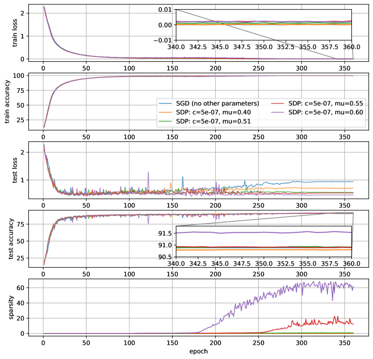
Figure 13: Learning trajectories of AltSDP and SGD for VGG-16 on CIFAR-10.

Here we first present the visualizing results for VGG-16 under different hyperparameters, which are used to check whether AltSDP reaches the same valley found by SGD. We train VGG16 on CIFAR-10 until nearly zero training loss using both SGD and AltSDP. We use the method of [43] to search for a quadratic Bézier curve of minimal training loss connecting the minima found by optimizers. In Figures 5-11, we respectively present the contour of training loss and testing error on the hyperplane for VGG-16 on CIFAR-10, where the hyperparameters are set according to that in Table 3 presented in the main paper. We recall the Table 3 in Table 5 here, where a more case when $c=5\times 10^{-7}$ and $\mu=0.6$ is added. We can see that AltSDP performs the structured directional pruning since the learned parameters of both SGD and AltSDP lie in the same flat minimum valley on the training loss landscape. In addition, Table 6 presents the details of the learning trajectories for VGG-16 on CIFAR-10, and Figure 13 presents the learning trajectories of AltSDP and SGD for VGG-16 on CIFAR-10.

Next, we present a visualizing example for WRN28$\times$10 to check whether AltSDP reaches the same valley found by SGD. We train WRN28$\times$10 on CIFAR-10 until nearly zero training loss using both SGD and AltSDP. In Figure 12, we present the contour of training loss and testing error on the hyperplane for WRN28$\times$10 on CIFAR-10. We can see that AltSDP performs the structured directional pruning since the learned parameters of both SGD and AltSDP lie in the same flat minimum valley on the training loss landscape. In addition, Table 7 presents the details of the learning trajectories for WRN28$\times$10 on CIFAR-10.

Dataset/Model	Learning	Decay Scheme	Batch Size	Hyper-parameters	Result
	Rate		Epoch
CIFAR-10/ResNet-56	0.05	[60, 160, 200, 220, 240]	64/260	$c=10^{-5}$, $\mu=0.55$	Table 1
		@[0.2, 0.2, 0.2, 0.2, 0.4]
CIFAR-10/VGG16	0.05	[60, 160, 200, 220, 240]	64/260	$c=10^{-5}$, $\mu=0.55$
		@[0.2, 0.2, 0.2, 0.2, 0.4]
CIFAR-100/ResNet-56	0.05	[60, 160, 200, 220, 240]	64/260	$c=10^{-5}$, $\mu=0.53$
		@[0.2, 0.2, 0.2, 0.2, 0.4]
CIFAR-10/VGG16	0.05	[60, 160, 200, 220, 240]	64/260	$c=10^{-5}$, $\mu=0.60$
		@[0.2, 0.2, 0.2, 0.2, 0.4]
CIFAR-10/ResNet-56	0.05	[100, 200, 220, 240, 260]	64/280	$c=10^{-5}$, $\mu=0.58$	Table 2
		@[0.2, 0.2, 0.2, 0.2, 0.4]

Table 4: Detail hyper-parameters to obtain results in Section 4.2.

	SGD	Structured directional pruning
	no other	$c=$ 5e-7	$c=$ 5e-7	$c=$ 5e-7	$c=$ 5e-7	$c=$ 8e-7	$c=$ 8e-7	$c=$ 8e-7
	parameters	$u=0.40$	$u=0.51$	$u=0.55$	$u=0.60$	$u=0.40$	$u=0.51$	$u=0.55$
Train loss	0.0001	0.0002	0.0012	0.0026	0.0022	0.0006	0.0023	0.0027
Test Acc.	0.9089	0.9080	0.9091	0.9090	0.9153	0.9077	0.9110	0.9127
Sparsity	0.0000	0.0000	0.0090	0.1242	0.7190	0.0084	0.4391	0.6767

Table 5: The effect of hyper-parameters

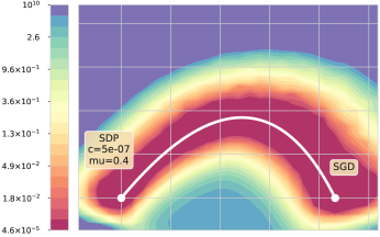
(a)

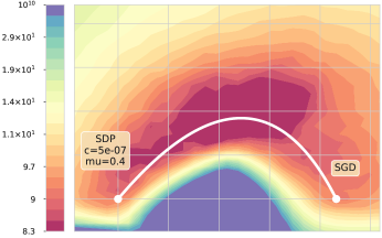
(b)

Figure 5: The contour of training loss and testing error on the hyperplane for VGG-16 on CIFAR-10. Sparsity = 0 for both AltSDP and SGD, where we set $c=5\times 10^{-7}$ and $\mu=0.4$. The test accuracy of AltSDP is 0.9080 while that of SGD is 0.9089. When the values of $c$ and $\mu$ are small, our AltSDP cannot obtain sparse results and suffer performance loss.

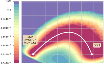
(a)

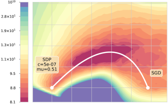
(b)

Figure 6: The contour of training loss and testing error on the hyperplane for VGG-16 on CIFAR-10. Sparsity = 0.009 for AltSDP and Sparsity = 0 for SGD, where we set $c=5\times 10^{-7}$ and $\mu=0.51$. The test accuracy of AltSDP is 0.9091 while that of SGD is 0.9089. When $\mu$ is slightly greater than 0.5, the model can become sparse and has good test accuracy.

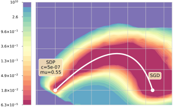
(a)

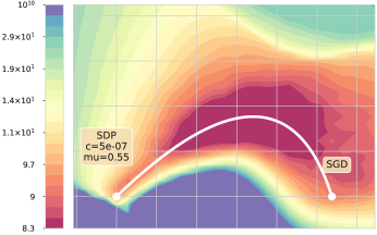
(b)

Figure 7: The contour of training loss and testing error on the hyperplane for VGG-16 on CIFAR-10. Sparsity = 0.124 for AltSDP and Sparsity = 0 for SGD, where we set $c=5\times 10^{-7}$ and $\mu=0.55$. The test accuracy of AltSDP is 0.9090 while that of SGD is 0.9089. When $\mu$ is slightly greater than 0.5, the model can become sparse and has good test accuracy.

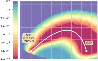
(a)

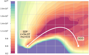
(b)

Figure 8: The contour of training loss and testing error on the hyperplane for VGG-16 on CIFAR-10. Sparsity = 0.719 for AltSDP and Sparsity = 0 for SGD, where we set $c=5\times 10^{-7}$ and $\mu=0.6$. The test accuracy of AltSDP is 0.9153 while that of SGD is 0.9089. As $\mu$ continues to grow larger, the model may become sparser. Here we find that, quite coincidentally, the test accuracy also improves, but as $\mu$ increases further, the model becomes sparser, which may eventually lead to performance degradation.

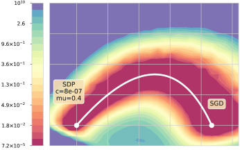
(a)

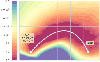
(b)

Figure 9: The contour of training loss and testing error on the hyperplane for VGG-16 on CIFAR-10. Sparsity = 0.008 for AltSDP and Sparsity = 0 for SGD, where we set $c=8\times 10^{-7}$ and $\mu=0.4$. The test accuracy of AltSDP is 0.9077 while that of SGD is 0.9089. When $c$ is increased, the model also becomes sparse, but the test accuracy decreases.

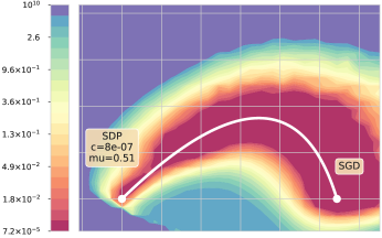
(a)

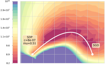
(b)

Figure 10: The contour of training loss and testing error on the hyperplane for VGG-16 on CIFAR-10. Sparsity = 0.439 for AltSDP and Sparsity = 0 for SGD, where we set $c=8\times 10^{-7}$ and $\mu=0.51$. The test accuracy of AltSDP is 0.9110 while that of SGD is 0.9089. When $\mu$ is slightly greater than 0.5 and $c$ increases, the model becomes sparse and the test accuracy also improves.

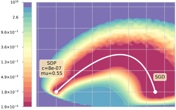
(a)

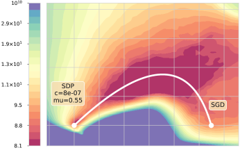
(b)

Figure 11: The contour of training loss and testing error on the hyperplane for VGG-16 on CIFAR-10. Sparsity = 0.677 for AltSDP and Sparsity = 0 for SGD, where we set $c=8\times 10^{-7}$ and $\mu=0.55$. The test accuracy of AltSDP is 0.9127 while that of SGD is 0.9089. When $\mu$ is slightly greater than 0.5 and $c$ increases, the model becomes sparse and the test accuracy also improves.

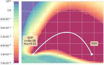
(a)

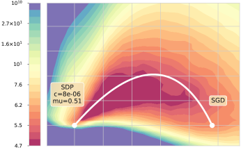
(b)

Figure 12: The contour of training loss and testing error on the hyperplane for WRN28$\times$10 on CIFAR-10. Sparsity = 0.489 for AltSDP and Sparsity = 0 for SGD, where we set $c=8\times 10^{-6}$ and $\mu=0.51$. The test accuracy of AltSDP is 0.9369 while that of SGD is 0.9418. When $\mu$ is slightly greater than 0.5 and $c$ further increases, the model becomes sparse, while the test accuracy is only reduced a little.

Epoch	Method	Training	Training	Testing	Sparsity
		Loss	Accuracy(%)	Accuracy(%)
60	SGD	0.1122	96.3280	87.2000	0.0000
	SDP($c=5\times 10^{-7}$, $\mu=0.40$)	0.1026	96.5320	88.0200	0.0000
	SDP($c=5\times 10^{-7}$, $\mu=0.51$)	0.1091	96.3160	87.4300	0.0000
	SDP($c=5\times 10^{-7}$, $\mu=0.55$)	0.1128	96.1500	87.7800	0.0000
	SDP($c=5\times 10^{-7}$, $\mu=0.60$)	0.1109	96.3660	84.7100	0.0000
	SDP($c=8\times 10^{-7}$, $\mu=0.40$)	0.1080	96.4580	88.3300	0.0000
	SDP($c=8\times 10^{-7}$, $\mu=0.51$)	0.1058	96.4920	84.9100	0.0000
	SDP($c=8\times 10^{-7}$, $\mu=0.60$)	0.1185	96.0960	88.1400	0.0000
120	SGD	0.0282	99.0680	88.3300	0.0000
	SDP($c=5\times 10^{-7}$, $\mu=0.40$)	0.0276	99.0820	88.9700	0.0000
	SDP($c=5\times 10^{-7}$, $\mu=0.51$)	0.0351	98.8400	89.6900	0.0000
	SDP($c=5\times 10^{-7}$, $\mu=0.55$)	0.0393	98.7480	89.1500	0.0000
	SDP($c=5\times 10^{-7}$, $\mu=0.60$)	0.0568	98.2820	88.6300	0.0043
	SDP($c=8\times 10^{-7}$, $\mu=0.40$)	0.0386	98.8860	89.1900	0.0000
	SDP($c=8\times 10^{-7}$, $\mu=0.51$)	0.0441	98.6060	88.0200	0.0017
	SDP($c=8\times 10^{-7}$, $\mu=0.60$)	0.0513	98.3940	88.0000	0.0042
180	SGD	0.0166	99.5040	89.7000	0.0000
	SDP($c=5\times 10^{-7}$, $\mu=0.40$)	0.0178	99.4440	89.1100	0.0000
	SDP($c=5\times 10^{-7}$, $\mu=0.51$)	0.0288	99.0740	89.1300	0.0036
	SDP($c=5\times 10^{-7}$, $\mu=0.55$)	0.0358	98.8660	88.4000	0.0048
	SDP($c=5\times 10^{-7}$, $\mu=0.60$)	0.0601	98.1660	88.0600	0.0150
	SDP($c=8\times 10^{-7}$, $\mu=0.40$)	0.0203	99.3360	89.3400	0.0000
	SDP($c=8\times 10^{-7}$, $\mu=0.51$)	0.0355	98.8800	88.7400	0.0055
	SDP($c=8\times 10^{-7}$, $\mu=0.60$)	0.0565	98.2220	89.1600	0.0464
240	SGD	0.0018	99.9480	90.5200	0.0000
	SDP($c=5\times 10^{-7}$, $\mu=0.40$)	0.0034	99.8880	90.1400	0.0000
	SDP($c=5\times 10^{-7}$, $\mu=0.51$)	0.0062	99.8240	90.6300	0.0047
	SDP($c=5\times 10^{-7}$, $\mu=0.55$)	0.0109	99.6920	90.3500	0.0109
	SDP($c=5\times 10^{-7}$, $\mu=0.60$)	0.0267	99.1940	89.1700	0.4466
	SDP($c=8\times 10^{-7}$, $\mu=0.40$)	0.0046	99.8700	90.2200	0.0029
	SDP($c=8\times 10^{-7}$, $\mu=0.51$)	0.0135	99.6180	90.6500	0.0734
	SDP($c=8\times 10^{-7}$, $\mu=0.60$)	0.0309	99.0800	90.5700	0.5221
300	SGD	0.0004	99.9820	90.7000	0.0000
	SDP($c=5\times 10^{-7}$, $\mu=0.40$)	0.0004	99.9920	90.7500	0.0000
	SDP($c=5\times 10^{-7}$, $\mu=0.51$)	0.0014	99.9880	90.8900	0.0081
	SDP($c=5\times 10^{-7}$, $\mu=0.55$)	0.0035	99.9380	90.9000	0.1010
	SDP($c=5\times 10^{-7}$, $\mu=0.60$)	0.0039	99.9200	91.2700	0.6490
	SDP($c=8\times 10^{-7}$, $\mu=0.40$)	0.0007	99.9920	90.9200	0.0036
	SDP($c=8\times 10^{-7}$, $\mu=0.51$)	0.0043	99.8940	91.1000	0.2136
	SDP($c=8\times 10^{-7}$, $\mu=0.60$)	0.0039	99.9380	91.2000	0.6496
360	SGD	0.0002	99.9960	90.8900	0.0000
	SDP($c=5\times 10^{-7}$, $\mu=0.40$)	0.0002	99.9940	90.8000	0.0000
	SDP($c=5\times 10^{-7}$, $\mu=0.51$)	0.0012	99.9820	90.9100	0.0090
	SDP($c=5\times 10^{-7}$, $\mu=0.55$)	0.0026	99.9640	90.9000	0.1242
	SDP($c=5\times 10^{-7}$, $\mu=0.60$)	0.0022	99.9760	91.5300	0.6197
	SDP($c=8\times 10^{-7}$, $\mu=0.40$)	0.0006	99.9920	90.7700	0.0084
	SDP($c=8\times 10^{-7}$, $\mu=0.51$)	0.0023	99.9700	91.1000	0.4391
	SDP($c=8\times 10^{-7}$, $\mu=0.60$)	0.0027	99.9640	91.2700	0.6767

Table 6: Details of the learning trajectories for VGG-16.

Epoch	Method	Training	Training	Testing	Sparsity
		Loss	Accuracy(%)	Accuracy(%)
40	SGD	0.0278	99.0920	90.5600	0.0000
	SDP($c=8\times 10^{-6}$, $\mu=0.55$)	0.3481	87.9880	69.4000	0.0000
80	SGD	0.0091	99.7140	91.7900	0.0000
	SDP($c=8\times 10^{-6}$, $\mu=0.55$)	0.3325	88.5620	57.8100	0.0678
120	SGD	0.0003	99.9960	93.9300	0.0000
	SDP($c=8\times 10^{-6}$, $\mu=0.55$)	0.2923	90.0820	83.4300	0.1945
160	SGD	0.0001	99.9980	94.1200	0.0000
	SDP($c=8\times 10^{-6}$, $\mu=0.55$)	0.1749	94.0400	86.5100	0.2438
200	SGD	0.0001	100.0000	94.1800	0.0000
	SDP($c=8\times 10^{-6}$, $\mu=0.55$)	0.0118	99.7720	93.6900	0.4890

Table 7: Details of the learning trajectories for WRN28$\times$10.

C.2 Experimental Results on MNIST Dataset

We also test AltSDP in a basic DNN model with 2 convolution layers and 2 full connection layers on the MNIST dataset. The learning rate is 0.1 at the beginning and mutiplied by 0.5 each 30 epochs. The results are listed in Table 8. We can see that when $\mu$ becomes larger, the model becomes sparser, which eventually leads to performance degradation.

Epoch	Method	Training	Training	Testing	Sparsity
		Loss	Accuracy(%)	Accuracy(%)
10	SGD	0.0050	99.8533	99.0400	0.0000
	SDP($c=1\times 10^{-6}$, $\mu=0.51$)	0.0063	99.8250	98.8600	0.0000
	SDP($c=1\times 10^{-6}$, $\mu=0.55$)	0.0079	99.7533	98.9700	0.0000
	SDP($c=1\times 10^{-6}$, $\mu=0.60$)	0.0074	99.7633	98.9400	0.0000
40	SGD	0.0000	100.0000	99.2300	0.0000
	SDP($c=1\times 10^{-6}$, $\mu=0.51$)	0.0005	100.0000	99.2400	0.0000
	SDP($c=1\times 10^{-6}$, $\mu=0.55$)	0.0012	99.9883	99.2500	0.0000
	SDP($c=1\times 10^{-6}$, $\mu=0.60$)	0.0055	99.8867	99.0400	0.2254
80	SGD	0.0000	100.0000	99.2300	0.0000
	SDP($c=1\times 10^{-6}$, $\mu=0.51$)	0.0031	99.9667	99.1600	0.2041
	SDP($c=1\times 10^{-6}$, $\mu=0.55$)	0.0038	99.9483	99.2000	0.3466
	SDP($c=1\times 10^{-6}$, $\mu=0.60$)	0.0045	99.9300	99.1400	0.4748
120	SGD	0.0000	100.0000	99.2300	0.0000
	SDP($c=1\times 10^{-6}$, $\mu=0.51$)	0.0019	99.9967	99.2300	0.3245
	SDP($c=1\times 10^{-6}$, $\mu=0.55$)	0.0023	99.9917	99.2700	0.4350
	SDP($c=1\times 10^{-6}$, $\mu=0.60$)	0.0032	99.9850	99.2200	0.5100
160	SGD	0.0000	100.0000	99.2300	0.0000
	SDP($c=1\times 10^{-6}$, $\mu=0.51$)	0.0021	100.0000	99.1300	0.3626
	SDP($c=1\times 10^{-6}$, $\mu=0.55$)	0.0025	99.9983	99.2700	0.4599
	SDP($c=1\times 10^{-6}$, $\mu=0.60$)	0.0034	99.9900	99.1300	0.5184
200	SGD	0.0000	100.0000	99.2300	0.0000
	SDP($c=1\times 10^{-6}$, $\mu=0.51$)	0.0023	100.0000	99.2100	0.3667
	SDP($c=1\times 10^{-6}$, $\mu=0.55$)	0.0026	100.0000	99.2700	0.4683
	SDP($c=1\times 10^{-6}$, $\mu=0.60$)	0.0035	99.9883	99.1500	0.5204

Table 8: Results on small dataset (MNIST)

References

• [1] Alex Krizhevsky, Ilya Sutskever, and Geoffrey E Hinton. Imagenet classification with deep convolutional neural networks. Advances in neural information processing systems, 25:1097–1105, 2012.
• [2] Kaiming He, Xiangyu Zhang, Shaoqing Ren, and Jian Sun. Deep residual learning for image recognition. In Proceedings of the IEEE conference on computer vision and pattern recognition, pages 770–778, 2016.
• [3] Li Deng and Dong Yu. Deep learning: methods and applications. Foundations and trends in signal processing, 7(3–4):197–387, 2014.
• [4] Andrew Brock, Jeff Donahue, and Karen Simonyan. Large scale gan training for high fidelity natural image synthesis. arXiv preprint arXiv:1809.11096, 2018.
• [5] Karen Simonyan and Andrew Zisserman. Very deep convolutional networks for large-scale image recognition. arXiv preprint arXiv:1409.1556, 2014.
• [6] Mikhail Belkin, Daniel Hsu, Siyuan Ma, and Soumik Mandal. Reconciling modern machine-learning practice and the classical bias–variance trade-off. Proceedings of the National Academy of Sciences, 116(32):15849–15854, 2019.
• [7] Shih-Kang Chao, Zhanyu Wang, Yue Xing, and Guang Cheng. Directional pruning of deep neural networks. In H. Larochelle, M. Ranzato, R. Hadsell, M. F. Balcan, and H. Lin, editors, Advances in Neural Information Processing Systems, volume 33, pages 13986–13998. Curran Associates, Inc., 2020.
• [8] Zhuang Liu, Mingjie Sun, Tinghui Zhou, Gao Huang, and Trevor Darrell. Rethinking the value of network pruning. arXiv preprint arXiv:1810.05270, 2018.
• [9] Carl Lemaire, Andrew Achkar, and Pierre-Marc Jodoin. Structured pruning of neural networks with budget-aware regularization. In Proceedings of the IEEE/CVF Conference on Computer Vision and Pattern Recognition, pages 9108–9116, 2019.
• [10] Jonathan Frankle and Michael Carbin. The lottery ticket hypothesis: Finding sparse, trainable neural networks. In International Conference on Learning Representations, 2018.
• [11] Shaohui Lin, Rongrong Ji, Chenqian Yan, Baochang Zhang, Liujuan Cao, Qixiang Ye, Feiyue Huang, and David Doermann. Towards optimal structured cnn pruning via generative adversarial learning. In Proceedings of the IEEE/CVF Conference on Computer Vision and Pattern Recognition, pages 2790–2799, 2019.
• [12] Babak Hassibi and David Stork. Second order derivatives for network pruning: Optimal brain surgeon. In S. Hanson, J. Cowan, and C. Giles, editors, Advances in Neural Information Processing Systems, volume 5. Morgan-Kaufmann, 1993.
• [13] David L Donoho. Compressed sensing. IEEE Transactions on information theory, 52(4):1289–1306, 2006.
• [14] Haiqin Yang, Zenglin Xu, Irwin King, and Michael R Lyu. Online learning for group lasso. In ICML, 2010.
• [15] Tsubasa Ochiai, Shigeki Matsuda, Hideyuki Watanabe, and Shigeru Katagiri. Automatic node selection for deep neural networks using group lasso regularization. In 2017 IEEE International Conference on Acoustics, Speech and Signal Processing (ICASSP), pages 5485–5489. IEEE, 2017.
• [16] Zhuang Liu, Jianguo Li, Zhiqiang Shen, Gao Huang, Shoumeng Yan, and Changshui Zhang. Learning efficient convolutional networks through network slimming. In Proceedings of the IEEE International Conference on Computer Vision, pages 2736–2744, 2017.
• [17] Yihui He, Xiangyu Zhang, and Jian Sun. Channel pruning for accelerating very deep neural networks. In Proceedings of the IEEE International Conference on Computer Vision, pages 1389–1397, 2017.
• [18] Yihui He, Ji Lin, Zhijian Liu, Hanrui Wang, Li-Jia Li, and Song Han. Amc: Automl for model compression and acceleration on mobile devices. In Proceedings of the European Conference on Computer Vision (ECCV), pages 784–800, 2018.
• [19] Zhuangwei Zhuang, Mingkui Tan, Bohan Zhuang, Jing Liu, Yong Guo, Qingyao Wu, Junzhou Huang, and Jinhui Zhu. Discrimination-aware channel pruning for deep neural networks. In S. Bengio, H. Wallach, H. Larochelle, K. Grauman, N. Cesa-Bianchi, and R. Garnett, editors, Advances in Neural Information Processing Systems, volume 31. Curran Associates, Inc., 2018.
• [20] Yang He, Guoliang Kang, Xuanyi Dong, Yanwei Fu, and Yi Yang. Soft filter pruning for accelerating deep convolutional neural networks. arXiv preprint arXiv:1808.06866, 2018.
• [21] Yang He, Ping Liu, Ziwei Wang, Zhilan Hu, and Yi Yang. Filter pruning via geometric median for deep convolutional neural networks acceleration. In Proceedings of the IEEE/CVF Conference on Computer Vision and Pattern Recognition, pages 4340–4349, 2019.
• [22] Hanyu Peng, Jiaxiang Wu, Shifeng Chen, and Junzhou Huang. Collaborative channel pruning for deep networks. In International Conference on Machine Learning, pages 5113–5122. PMLR, 2019.
• [23] Tao Zhuang, Zhixuan Zhang, Yuheng Huang, Xiaoyi Zeng, Kai Shuang, and Xiang Li. Neuron-level structured pruning using polarization regularizer. In H. Larochelle, M. Ranzato, R. Hadsell, M. F. Balcan, and H. Lin, editors, Advances in Neural Information Processing Systems, volume 33, pages 9865–9877. Curran Associates, Inc., 2020.
• [24] Wenxiao Wang, Cong Fu, Jishun Guo, Deng Cai, and Xiaofei He. Cop: Customized deep model compression via regularized correlation-based filter-level pruning. In Proceedings of the Twenty-Eighth International Joint Conference on Artificial Intelligence, IJCAI-19, pages 3785–3791. International Joint Conferences on Artificial Intelligence Organization, 7 2019.
• [25] Behrooz Ghorbani, Shankar Krishnan, and Ying Xiao. An investigation into neural net optimization via hessian eigenvalue density. In International Conference on Machine Learning, pages 2232–2241. PMLR, 2019.
• [26] Vardan Papyan. Measurements of three-level hierarchical structure in the outliers in the spectrum of deepnet hessians. In International Conference on Machine Learning, pages 5012–5021. PMLR, 2019.
• [27] Shih-Kang Chao and Guang Cheng. A generalization of regularized dual averaging and its dynamics. arXiv preprint arXiv:1909.10072, 2019.
• [28] Francesco Orabona, Koby Crammer, and Nicolo Cesa-Bianchi. A generalized online mirror descent with applications to classification and regression. Machine Learning, 99(3):411–435, 2015.
• [29] Lin Xiao. Dual averaging method for regularized stochastic learning and online optimization. Advances in Neural Information Processing Systems, 22:2116–2124, 2009.
• [30] Sanjeev Arora, Nadav Cohen, and Elad Hazan. On the optimization of deep networks: Implicit acceleration by overparameterization. In International Conference on Machine Learning, pages 244–253. PMLR, 2018.
• [31] Gerald Teschl. Ordinary differential equations and dynamical systems, volume 140. American Mathematical Soc., 2012.
• [32] Simon S Du, Jason D Lee, and Yuandong Tian. When is a convolutional filter easy to learn? In International Conference on Learning Representations, 2018.
• [33] Xiao Zhang, Yaodong Yu, Lingxiao Wang, and Quanquan Gu. Learning one-hidden-layer relu networks via gradient descent. In The 22nd International Conference on Artificial Intelligence and Statistics, pages 1524–1534. PMLR, 2019.
• [34] Guy Gur-Ari, Daniel A Roberts, and Ethan Dyer. Gradient descent happens in a tiny subspace. arXiv preprint arXiv:1812.04754, 2018.
• [35] Suriya Gunasekar, Jason Lee, Daniel Soudry, and Nathan Srebro. Characterizing implicit bias in terms of optimization geometry. In International Conference on Machine Learning, pages 1832–1841. PMLR, 2018.
• [36] Yann LeCun, Léon Bottou, Yoshua Bengio, and Patrick Haffner. Gradient-based learning applied to document recognition. Proceedings of the IEEE, 86(11):2278–2324, 1998.
• [37] Alex Krizhevsky, Geoffrey Hinton, et al. Learning multiple layers of features from tiny images. Citeseer, 2009.
• [38] Adam Paszke, Sam Gross, Francisco Massa, Adam Lerer, James Bradbury, Gregory Chanan, Trevor Killeen, Zeming Lin, Natalia Gimelshein, Luca Antiga, Alban Desmaison, Andreas Kopf, Edward Yang, Zachary DeVito, Martin Raison, Alykhan Tejani, Sasank Chilamkurthy, Benoit Steiner, Lu Fang, Junjie Bai, and Soumith Chintala. Pytorch: An imperative style, high-performance deep learning library. In H. Wallach, H. Larochelle, A. Beygelzimer, F. d Alché-Buc, E. Fox, and R. Garnett, editors, Advances in Neural Information Processing Systems, volume 32. Curran Associates, Inc., 2019.
• [39] Timur Garipov, Pavel Izmailov, Dmitrii Podoprikhin, Dmitry P Vetrov, and Andrew G Wilson. Loss surfaces, mode connectivity, and fast ensembling of dnns. In S. Bengio, H. Wallach, H. Larochelle, K. Grauman, N. Cesa-Bianchi, and R. Garnett, editors, Advances in Neural Information Processing Systems, volume 31. Curran Associates, Inc., 2018.
• [40] Quynh Nguyen. On connected sublevel sets in deep learning. In International Conference on Machine Learning, pages 4790–4799. PMLR, 2019.
• [41] Felix Draxler, Kambis Veschgini, Manfred Salmhofer, and Fred Hamprecht. Essentially no barriers in neural network energy landscape. In International conference on machine learning, pages 1309–1318. PMLR, 2018.
• [42] Haowei He, Gao Huang, and Yang Yuan. Asymmetric valleys: Beyond sharp and flat local minima. In H. Wallach, H. Larochelle, A. Beygelzimer, F. d Alché-Buc, E. Fox, and R. Garnett, editors, Advances in Neural Information Processing Systems, volume 32. Curran Associates, Inc., 2019.
• [43] Timur Garipov, Pavel Izmailov, Dmitrii Podoprikhin, Dmitry Vetrov, and Andrew Gordon Wilson. Loss surfaces, mode connectivity, and fast ensembling of dnns. arXiv preprint arXiv:1802.10026, 2018.
• [44] Albert Benveniste, Michel Métivier, and Pierre Priouret. Adaptive algorithms and stochastic approximations, volume 22. Springer Science & Business Media, 2012.
• [45] MSP Eastham. The asymptotic solution of linear differential systems. Mathematika, 32(1):131–138, 1985.
• [46] Amnon Pazy. Semigroups of linear operators and applications to partial differential equations, volume 44. Springer Science & Business Media, 2012.