Experimental and theoretical characterization of a non-equilibrium steady state of a periodically driven qubit

Abstract

Periodically driven dynamics of open quantum systems is very interesting because typically non-equilibrium steady state is reached, which is characterized by a non-vanishing current. In this work, we study time discrete and periodically driven dynamics experimentally for a single photon that its coupled to its environment. We develop a comprehensive theory which explains the experimental observations and offers an analytical characterization of the non-equilibrium steady states of the system. We demonstrate that the periodic driving and the properties of the environment can be engineered in such a way that there is asymptotically non-vanishing bidirectional information flow between the open system and the environment.

Introduction.—

In realistic situations quantum systems are not isolated from the surrounding environment Alicki and Lendi (1987). The coupling of the open system to the external world dynamically creates correlations between the open system and it’s environment. These then lead to typically adversary effects such as decoherence and dissipation on the level of the reduced state of the open system Breuer et al. (2002).

To cope with this unavoidable interaction one can try to perform quantum operations on a time scale that is faster than the decoherence and dissipation timescale Steane et al. (2014); Nielsen and Chuang (2011), so that negative environmental effects do not degrade the quantum state. Another route is to protect the quantum state is by using reservoir engineering to modify the environment Diehl et al. (2008) or to do some local control operations on the open system in hope to drive the system into decoherence free subspace Yi et al. (2009), for example. Recent years, significant technological advancements have made it possible to realize both strategies in various different experimental platforms, such as, ion traps  Schäfer et al. (2018); Steane et al. (2014); Choi et al. (2014), NV-centers Putz et al. (2014) and single photons in free space Liu et al. (2018), to name a few.

From both experimental and theoretical point of view, periodical local control strategies, leading to so called Floquet dynamics Carollo et al. (2020); Vogl et al. (2019), for open quantum systems are very interesting. For example, the open system typically will not reach a stationary state but rather the local driving forces the system asymptotically to a non-equilibrium steady state, which is characterized by non-vanishing current Karevski and Platini (2009); Bordia et al. (2017). Another interesting class of system, where effects similar to a periodical driving occur are discrete time quantum walks Aharonov et al. (1993), where the time discrete nature of the dynamics leads to the Floquet theory and interesting phenomena ranging from topologically protected modes Kitagawa et al. (2010) to controlled transition from ballistic spread to localization Schreiber et al. (2011) can be observed. Hardly any analytical results characterizing the asymptotic non-stationary steady states occurring in these generally driven and dissipative systems exist.

In this Letter we study time discrete and periodically driven dynamics both theoretically and experimentally for a single photon that its coupled to its environment. The polarization degrees of freedom of the photon act as an open system and the frequency degree of freedom will serve as the environment, as in Liu et al. (2011, 2018) We investigate the long time dynamics dynamics of the system experimentally and reveal signatures of the non-equilibrium steady state from the data based on the comprehensive theory we develop. In particular, we show that the periodic driving and the properties of the environment can be engineered in such a way that there is asymptotically non-vanishing bidirectional exchange of information between the open system and the environment leading to unbounded non-Markovianity.

Experimental setup—

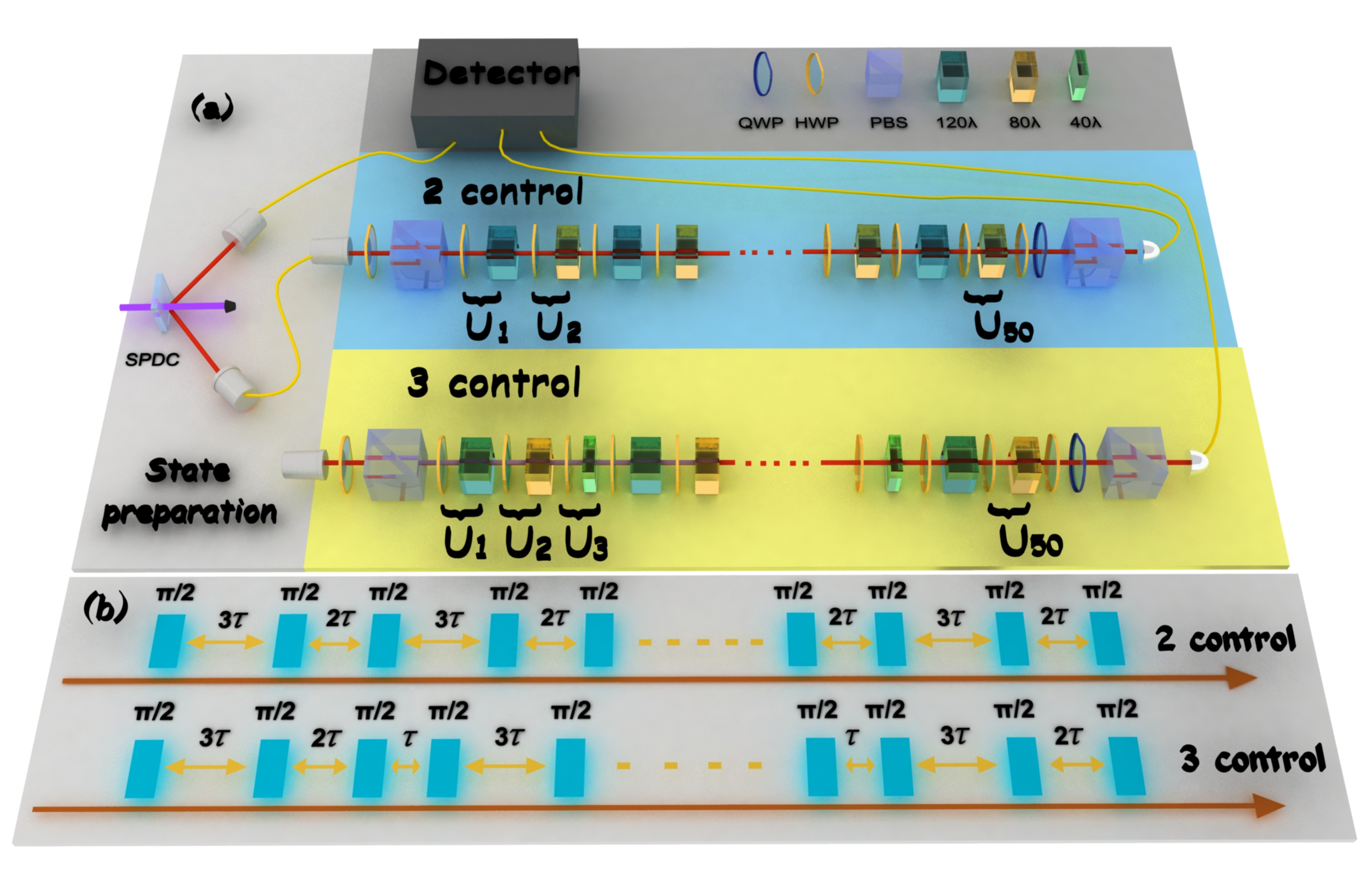
Figure 1: Experimental setup for testing the quantum non-equilibrium steady state. (a) In our experiment, we realize the unitary control and decoherence with a half-wave plate (HWP) and a quartz plate which is called a operation unit $U$. There are in total of 50 sets of operation units in our experiment. (b) Schematic picture of the experiment. We show two dynamic progresses leading to the non-equilibrium steady state which we call two controls and three controls in our experiment. Two kinds of operation units are used in the case of two controls to realize the non-equilibrium steady state. For the case of three controls, three kinds of operation units are used. Legend: QWP, quarter-wave plate; HWP, half-wave plate; PBS, polarizing beam splitter; 3 kinds of quartz plates with different effective path difference: $\Delta L=120\lambda$, $\Delta L=80\lambda$ and $\Delta L=40\lambda$.

Our experimental setup is shown in Fig. 1. In our experiment, a type-II beta-barium-borate (BBO, $9.0\times 7.0\times 1.0$ $mm^{3}$, $\theta=41.44^{\circ}$) crystal is pumped by a frequency-doubled femtosecond pulse (400 nm, 76 MHz repetition rate) from a mode-locked Ti:sapphire laser to generate the degenerate photon pairs. After passing through the interference filter (IF, $\Delta\lambda$ = 3 nm, $\lambda$ = 800 nm), the photon pairs generated in the spontaneous parametric down conversion (SPDC) process are coupled into single-mode fibers separately. A single-photon state is prepared by triggering on one of the two photons, and the coincidence counting rate collected by the avalanche photodiodes (APDs) is about $1.8\times 10^{5}$ in 60 s.

As shown in Fig. 1, the single photon states are initialized into state $|H\rangle$ by the first polarizing beam splitter. We use a half-wave plate (HWP) and a quartz plate to realize the unitary control and decoherence. The combination of a half-wave plate and a quartz plate is called a operation unit $U$. There are in total of 50 sets of operation units in each of our experiment. The refraction indices $n_{H}$ and $n_{V}$ of the quartz plates are 1.5473 and 1.5384, respectively. We have three kinds of quartz plates with different thicknesses, corresponding to different dephasing strengths. We express the thicknesses of the quartz plates in terms of effective path difference, $\Delta L=40\lambda$, $\Delta L=80\lambda$ and $\Delta L=120\lambda$, which correspond to the thicknesses of 3.556 mm, 7.111 mm and 10.667 mm, respectively. Different angles of the half-wave plates lead to different values of the parameter $\eta$ and different local control schemes. The value $\eta=0.5$ use in each operation unit $U_{i}$ corresponds to a unitary rotation of the polarization of the photon effected by a half-wave plate set in angle of $22.5^{\circ}$ incident to the photon. At the final step, we make a quantum state tomography for the single photon states after each step with a polarizing beam splitter, a half-wave plate and a quarter-wave plate.

For the case of two controls, two kinds of quartz plates are used, $\Delta L=120\lambda$ and $\Delta L=80\lambda$ for the operation units $U_{1}$ and $U_{2}$, respectively. We stack in total 50 operation units cyclically $U_{2}U_{1}\cdots U_{2}U_{1}$ in our experiment.

For the case of three controls, three kinds of quartz plates are used. In operation unit $U_{1},\,U_{2}$ and $U_{3}$ the thicknesses are $\Delta L=120\lambda$, in $U_{2}$ $\Delta L=80\lambda$ and $\Delta L=40\lambda$, respectively. We stack in total 50 operation units cyclically $U_{2}U_{1}U_{3}U_{2}U_{1}\cdots U_{3}U_{2}U_{1}$ in our experiment. Note here that $50\mod 3=2$ and therefore the $50$th operation unit is $U_{2}$.

Experimental results.—

In the case of two controls, we have initialized the polarization to state $|\varphi\rangle=|H\rangle$. After short initial transient the polarization oscillates between two values, as can be seen in Fig. 2 a). Our theoretical prediction fits well to the experiment. In panel b) of Fig. 2 we use three controls and find a good match between the theory and experiment. In the case of three controls the asymptotic dynamics oscillates between three different polarization states as can be seen from Fig. 3 a) and b). In both the two and three control cases the dynamics is confined to the plane $y=0$ cutting the Bloch sphere by a suitable choice of the initial state. Interesting features of this rather simple looking dynamics can be revealed from the theory developed next.

Theory.—

Quantum mechanical state of a single photon wave packet is an element of $\mathcal{H}=\mathcal{H}_{S}\otimes\mathcal{H}_{E}=\mathbb{C}^{2}\otimes L^{2}()$, where the polarization and the frequency of the photon correspond to the first and to the second Hilbert space, respectively. The photon is prepared initially into a pure state $|\Psi\rangle=\int{\rm d}\omega\,\chi(\omega)|\varphi\rangle\otimes|\omega\rangle$, in such a way, that the frequency spectrum of the photon is a Gaussian

$$|\chi(\omega)|^{2}=\frac{1}{\sqrt{2\pi}\sigma}e^{-(\omega-\mu)^{2}/2\sigma^{2}},$$ (1)

with central frequency $\mu$ and standard deviation $\sigma$. The photon propagates trough a set of linear optical elements that sequentially rotate its polarization state and couple the polarization and frequency degrees of freedom. Such a procedure defines the following dynamical map that acts on the polarization state of the photon

$$\Phi_{n}[\rho_{0}]= \int_{\rm d}\omega\,|\chi(\omega)|^{2}\prod_{i=0}^{n-1}{\mathcal{U}}_{n-i}(\omega)[\rho_{0}],$$ (2a)

$${\mathcal{U}}_{i}(\omega)[\rho]= U_{i}(\omega)\cdot(C_{\eta_{i}}\otimes\mathbbm{1}_{E})\rho(C_{\eta_{i}}\otimes\mathbbm{1}_{E})^{\dagger}\cdot U_{i}(\omega)^{\dagger}$$ (2b)

where $U_{i}(\omega)=e^{in_{1}\omega L_{i}/c}|1\rangle\langle 1|+e^{in_{2}\omega L_{i}/c}|2\rangle\langle 2|$ couples the polarization and frequency degrees of freedom and $C_{\eta_{i}}=\sqrt{\eta_{i}}\sigma_{z}+\sqrt{1-\eta_{i}}\sigma_{x}$ rotates the polarization. $0\leq\eta_{i}\leq 1$ parametrize the rotations, $n_{i}$,$L_{i}$ and $c$ parametrize the couplings between the open system and it’s environment corresponding to the indices of refraction and length of a quartz plate where $c$ is the speed of light. We immediately see that the map is unital $\Phi_{n}(\mathbbm{1})=\mathbbm{1}$. From now on we set $\eta_{i}=\eta$ for each step and $\eta=0.5$ whenever numerical values are required.

In the Bloch picture $\rho=\frac{1}{2}(\mathbbm{1}+\mathbf{a}\cdot\boldsymbol{\sigma})$ the unitary operators are

$${\mathcal{U}}(\omega)= \left(\begin{array}[]{ccc}\beta\cos\frac{\Delta n\omega L}{c}&-\beta\sin\frac{\Delta n\omega L}{c}&\alpha\\ -\sin\frac{\Delta n\omega L}{c}&-\cos\frac{\Delta n\omega L}{c}&0\\ \alpha\cos\frac{\Delta n\omega L}{c}&-\alpha\sin\frac{\Delta n\omega L}{c}&-\beta\end{array}\right)$$ (3d)

$$C_{\eta}= \left(\begin{array}[]{ccc}\beta&0&\alpha\\ 0&-1&0\\ \alpha&0&-\beta\end{array}\right),$$ (3h)

$$U(\omega)= \left(\begin{array}[]{ccc}\cos\frac{\Delta n\omega L}{c}&-\sin\frac{\Delta n\omega L}{c}&0\\ \sin\frac{\Delta n\omega L}{c}&\cos\frac{\Delta n\omega L}{c}&0\\ 0&&1\end{array}\right)$$ (3l)

where $\Delta n=n_{1}-n_{2}$, $\beta=1-2\eta$ and $\alpha=2\sqrt{(1-\eta)\eta}$. We see that the unitary operators are mapped to orthogonal matrices acting on ³. Initial Bloch vector $\mathbf{a}$ is mapped to $\mathbf{a}_{n}=\int{\rm d}\omega\,|\chi(\omega)|^{2}\prod_{i=0}^{n-1}{\mathcal{U}}_{n-i}(\omega)\mathbf{a}.$ Further, we make a change of variables $t=\tan\frac{\Delta nL\omega}{c}$, such that the trigonometric functions are mapped to polynomials in $t$. The details of this transformation are in the Supplementary Material Sun et al. .

Open system dynamics leading to non-equilibrium steady state can be engineered if we periodically vary the linear optical elements. Let $T\in\mathbb{Z}_{+}$ be a length of such a period. The asymptotic dynamical maps $\tilde{\Phi}_{Tm+K}$, where $0\leq K<T$ can be seen as a integer valued phase of the periodic driving, characterize the asymptotic dynamics. Maps $\tilde{\Phi}_{Tm+k}$ are obtained using generating function techniques and asymptotic analysis Flajolet and Sedgewick (2009), which we now present.

Let $\{H_{n}\}_{n=0}^{\infty}$ be a family of orthogonal matrices acting on ³. Further, matrices $H_{n}$ satisfy the following recursion relation

$$H_{n+1}=WH_{n},\,\,\forall n\geq 0, H_{0}=A,$$ (4)

where $A$ is arbitrary initial condition and $W$ is an orthogonal matrix. Then we define the $z$-transform as $H(z)=\sum_{n=0}^{\infty}z^{n}H_{n}$, where $z\in\mathbb{C}$.

Multiplying both sides of Eq. (4) with $z^{n}$ and performing the sum $\sum_{n=1}^{\infty}$ formally on both sides, we obtain

$$H(z)= (\mathbbm{1}-zW)^{-1}A.$$ (5)

By Cramers rule we know that

$$(\mathbbm{1}-zW)^{-1}=\frac{\mathsf{adj}(\mathbbm{1}-zW)}{\mathsf{det}(\mathbbm{1}-zW)},$$ (6)

where $\mathsf{adj}(\cdot)$ denotes the adjungate matrix. $W$ is orthogonal matrix acting on ³ and therefore it has eigenvalue $\lambda=1$. Since determinant is a product of eigenvalues, we see that all the matrix elements of $H(z)$ have a simple pole at $z=1$. On the other hand, we have the following asymptotic relation Flajolet and Sedgewick (2009)

$$\lim_{n\to\infty}W^{n}A\sim\lim_{z\to 1}(1-z)H(z)=\mathsf{Res}(H(z),z=1),$$ (7)

which can be easily seen by expanding the geometric series and telescoping the resulting expression. The $\mathsf{Res}(H(z),z=z_{0})$ corresponds to element-wise residue operation.

Suppose now that we have a situation where the matrix $H_{n}$ satisfies a periodic recursion relation with period $T$. First we define an operator

$$\mathsf{cyc}(W_{T}W_{T-1}\cdots W_{1})=W_{1}W_{T}\cdots W_{2},$$ (8)

that is $\mathsf{cyc}$ shifts the operators cyclically to the right. For example $\mathsf{cyc}^{2}(ABC)=\mathsf{cyc}(CAB)=BAC$ and so on. Then we can write for any $0\leq K<T$

$$H_{mT+K}= \mathsf{cyc}^{K}(W_{T}\cdots W_{1})^{m}W_{K}W_{K-1}\cdots W_{1}A.$$ (9)

Meaning of the above formula is easy to understand. Integer $K$ corresponds to the phase of the evolution over a single period of length $T$.

This observation opens up a possibility to have maps that do not have a stationary state but rather a non-equilibrium steady state. This can be seen by applying Eq. (5) to the periodically driven evolution (9). Namely, if there exist a set of integer phases $S$, such that the asymptotic limit maps differ, ie.

$$\lim_{n\to\infty}\mathsf{cyc}^{K}(W_{T}\cdots W_{1})^{n}W_{K}\cdots W_{1}A$$

$$\neq\lim_{n\to\infty}\mathsf{cyc}^{K^{\prime}}(W_{T}\cdots W_{1})^{n}W_{K^{\prime}}\cdots W_{1}A,$$ (10)

for any $K^{\prime},K^{\prime}\in S$, then asymptotically we have $|S|$ phase dependent limit maps. $|S|$ corresponds to the number of elements in the set $S$.

Application of the general theory to two and three controls—

For the case of two controls, for which $(\Delta nL_{1})/(\Delta nL_{2})=3/2$, where $\Delta nL_{i}$ is the dephasing strength and $\eta_{1}=\eta_{2}=1/2$, we find that the asymptotic dynamical map takes the following form

$$\tilde{\Phi}_{2m} =\left(\begin{array}[]{ccc}0.635946&0&0.394485\\ 0&0.114589&0\\ 0.394485&0&0.249465\end{array}\right),$$ (11d)

$$\tilde{\Phi}_{2m+1} =\left(\begin{array}[]{ccc}0.394485&0&0.249465\\ 0&0.114589&0\\ 0.635946&0&0.394485\end{array}\right).$$ (11h)

In this case, all eigenvalues of both asymptotic maps are non-zero and non-degenerate. Initial states with Bloch vector $\mathbf{a}=a\mathbf{e}_{y}$, with $|a|\leq 1$ map asymptotically to $\mathbf{a}\mapsto\lambda_{y}^{(2m)}a\mathbf{e}_{y}=\lambda_{y}^{(2m+1)}a\mathbf{e}_{y}$, which is the same state for even and odd number of steps because $\lambda_{y}^{(2m)}=\lambda_{y}^{(2m+1)}=0.114589$. The two dimensional subspace orthogonal to $\mathbf{e}_{y}$ is spanned by vectors $\mathbf{x}_{1}^{(2m)}$ and $\mathbf{x}_{3}^{(2m)}$, which correspond to first and third columns of the matrix $\tilde{\Phi}_{2m}$. In this subspace the asymptotic dynamics corresponds to $\sigma_{x}$ i.e. $\mathbf{x}_{1/3}^{(2m+1)}=\sigma_{x}\mathbf{x}_{1/3}^{(2m)}$. We can conclude that in the two control case (i) the purity stays asymptotically constant since $\sigma_{x}$ is unitary and (ii) the initial states that have support in the subspace orthogonal to $\mathbf{e}_{y}$ oscillate asymptotically with the same period as the driving. The asymptotic “flipping” dynamics is clearly visible in Fig. 2 a).

For the case of three controls, which satisfy $(\Delta nL_{1})/(\Delta nL_{2})=3/2$, $(\Delta nL_{2})/(\Delta nL_{3})=2$ and $\eta_{1}=\eta_{2}=\eta_{3}=1/2$, we find that the asymptotic propagators have the following structure

$$\tilde{\Phi}_{3m}(t)= \left(\begin{array}[]{ccc}0.363253&0&0.331023\\ 0&0.0590277&0\\ 0.331023&0&0.577719\end{array}\right),$$ (12d)

$$\tilde{\Phi}_{3m+1}(t)= \left(\begin{array}[]{ccc}0.350767&0&0.399416\\ 0&0.127151&0\\ 0.363253&0&0.331023\end{array}\right),$$ (12h)

$$\tilde{\Phi}_{3m+2}(t)= \left(\begin{array}[]{ccc}0.331023&0&0.577719\\ 0&-0.0386657&0\\ 0.350767&0&0.399416\end{array}\right).$$ (12l)

The asymptotic maps $\tilde{\Phi}_{3m+i}$, $0\leq i<3$ can be all decomposed to one dimensional subspace spanned by $\mathbf{e}_{y}$ and its orthogonal complement. We denote the eigenvalues as $\lambda_{y}=\lambda_{y}^{(3m)}$, $\lambda_{y}^{\prime}=\lambda_{y}^{(3m+1)}$ and $\lambda_{y}^{\prime\prime}=\lambda_{y}^{(3m+2)}$. We have $|\lambda_{y}^{\prime\prime}|<|\lambda_{y}|<|\lambda_{y}^{\prime}|$, which shows that there exists initial states whose purity changes asymptotically. Namely, initial states given by Bloch vector $\mathbf{a}=a\mathbf{e}_{y}$, where $|a|\leq 1$. The orthogonal complements are spanned by vectors $\mathbf{x}_{1/3}$, $\mathbf{x}_{1/3}^{\prime}$ and $\mathbf{x}_{1/3}^{\prime\prime}$ corresponding to the first- and third column of maps  (12d),(12h) and (12l). Suppose we consider initial state $\mathbf{a}=(1/\sqrt{2})(\mathbf{e}_{x}+\mathbf{e}_{z})\perp\mathbf{e}_{y}$. We see that $||\tilde{\Phi}_{3m+1}\mathbf{a}||<||\tilde{\Phi}_{3m}\mathbf{a}||<||\tilde{\Phi}_{3m+2}\mathbf{a}||$, thus we see that the purity changes also for vectors in the orthogonal complement of $\mathbf{e}_{y}$. The period of three steps is clearly visible in Fig. 2 b) and the evolution of purity in Fig. 3 b).

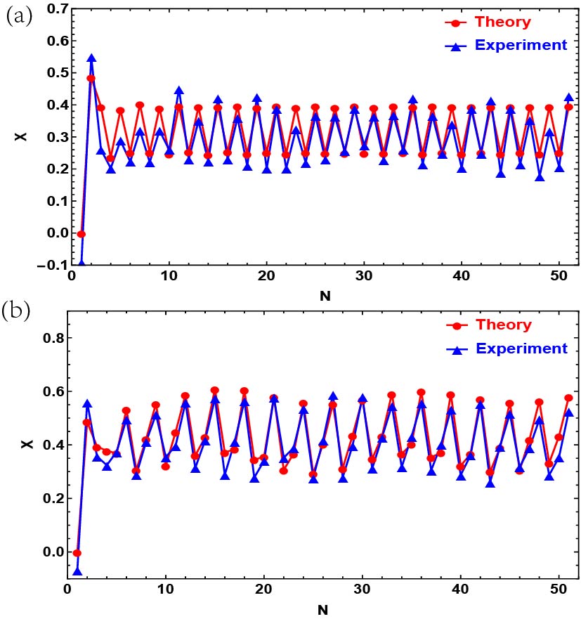
Figure 2: Evolution of the polarization state of the photon for the initial state $|\varphi\rangle=|H\rangle$ after 50 steps. (a)Theoretical and experimental results for two controls. (b) Theoretical and experimental results for three controls.

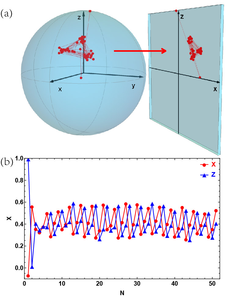
Figure 3: Evolution of the polarization state of the photon for the initial state $|\varphi\rangle=|H\rangle$ for three controls. (a) Evolution of the polarization state in bloch sphere. (b) Dynamics for the x and z components of the bloch vector for three controls.

Maximal visibility.—

To experimentally observe the non-stationary steady state, the initial state should be chosen such that its visibility is maximal. This means that the volume spanned by the points in the limit cycle is maximal. The volume is expressed as a function $f_{V}(\mathbf{a})=f_{V}(\theta,\varphi)$, where $\mathbf{a}=(\cos\varphi\sin\theta,\sin\varphi\sin\theta,\cos\theta)^{T}$ is the Bloch vector of the initial state. The extremal solutions are found when $\partial_{\theta}f_{V}=\partial_{\varphi}f_{V}=0$. The extremals correspond to maximums if the Hessian $H(f_{V})$, that is the matrix formed from the second order partial derivatives, is negative definite.

For two point cycle, the volume is the Euclidean distance between the two asymptotic states $f_{V}^{(2)}(\theta,\varphi)=||(\Phi_{2m}-\Phi_{2m-1})\mathbf{a}||^{2}$, which is to be maximized.

For three point cycle the volume is the area spanned by the parallelogram formed by the three asymptotic endpoint vectors. To compute it, we first label the asymptotic states as $\mathbf{x}=\Phi_{3m}\mathbf{a}$, $\mathbf{x}^{\prime}=\Phi_{3m+1}\mathbf{a}$ and $\mathbf{x}^{\prime\prime}=\Phi_{3m+2}\mathbf{a}$. Then we define $\mathbf{u}=\mathbf{x}^{\prime}-\mathbf{x}$ and $\mathbf{k}=\mathbf{x}^{\prime\prime}-\mathbf{x}^{\prime}$. Now the area spanned by the parallelogram is $||\mathbf{u}\times\mathbf{k}||$ which reads $f_{V}^{(3)}(\theta,\varphi)=\frac{1}{2}||\mathbf{x}\times\mathbf{x}^{\prime}+\mathbf{x}^{\prime}\times\mathbf{x}^{\prime\prime}+\mathbf{x}^{\prime\prime}\times\mathbf{x}||$. When given the asymptotic maps the volumes $f_{V}^{(2)}$ and $f_{V}^{(3)}$ are very easy to maximize. We present theoretical and experimental results for the maximal visibility initial state in the Supplemental Material Sun et al. .

Maximal non-Markovianity.—

The non-stationary steady state can lead to unbounded non-Markovianity of the dynamics measured by the BLP-measure Breuer et al. (2009). For example, in the case of asymptotic three cycle, Eqs. (12d-12l), we consider pure state pairs initially polarized in the $y$-direction $\rho_{y}^{\pm}=\frac{1}{2}(\mathbbm{1}\pm\mathbf{e}_{y}\boldsymbol{\sigma})$, for which $D(\rho_{y}^{+},\rho_{y}^{-})=1$. We use the following shorthand notation $D_{m}^{y}=D(\rho_{y}^{+}(m),\rho_{y}^{-}(m))$. We see that asymptotically

$$D_{3m+1}^{y}-D_{3m}^{y} =|\lambda_{y}^{\prime}|-|\lambda_{y}|>0,$$

$$D_{3m+2}^{y}-D_{3m+1}^{y} =|\lambda_{y}^{\prime\prime}|-|\lambda_{y}^{\prime}|<0,$$ (13)

$$D_{3m}^{y}-D_{3m+2}^{y} =|\lambda_{y}|-|\lambda_{y}^{\prime\prime}|>0.$$

The asymptotic growth emerges from the first and the second term. The trace distance can be written as a maximization over all positive operators

$$D(\rho_{1},\rho_{2})=\max_{F^{\prime}}\text{tr}\left\{F^{\prime}(\rho_{1}-\rho_{2})\right\},$$ (14)

$0<F\leq\mathbbm{1}$ Nielsen and Chuang (2011). In the running example the positive operator that maximizes Eq. (14) for all points in the asymptotic cycle corresponds to either of the POVM’s $F_{*}^{\prime}=\frac{1}{2}(\mathbbm{1}\pm{\rm e}_{y}\boldsymbol{\sigma})$. Therefore, the lower bound for non-Markovianity is obtained from the asymptotic oscillations of the polarization in the $y$-direction.

Largest asymptotic growth of non-Markovianity is obtained for orthogonal initial state pairs that asymptotically have largest change in the purity during one cycle. The proof of the claim is the following. For qubit states the trace distance is proportional to the Euclidean norm of Bloch vector corresponding to the difference state $D(\rho_{1},\rho_{2})=\frac{1}{2}||\mathbf{a}_{1}-\mathbf{a}_{2}||$. The non-Markovianity measure is maximized for orthogonal initial state pair, for which the initial Bloch vectors are anti-podal, $\mathbf{a}_{0}^{\pm}$ Wissmann et al. (2012). Since, the dynamical map is linear, the evolution of the anti-podal state pair has a reflection symmetry, i.e. $\mathbf{a}_{m}^{+}=-\mathbf{a}_{m}^{-}$. Therefore, $D_{m}^{\pm}=D(\mathbf{a}_{m}^{+},\mathbf{a}_{m}^{-})=||\mathbf{a}_{m}^{\pm}||$. Length of the Bloch vector corresponds to the purity of the state. Then clearly, we have largest asymptotic growth of non-Markovianity for initial states that have largest purity changes asymptotically. In general the different asymptotic states during one cycle are not parallel i.e. $\mathbf{a}_{m}\nparallel\mathbf{a}_{m+k}$. Therefore we can not find a single observable that would give the trace distance for the optimal initial state at any point in the asymptotic cycle.

Conclusions.—

Hardly any analytical results characterizing the asymptotic non-stationary steady states occurring in these generally driven and dissipative systems exist. We have studied time discrete and periodically driven dynamics both theoretically and experimentally for a single photon that its coupled to its environment. We have characterized analytically the non-equilibrium steady states and experimentally verified our theoretical results. We show that the periodic driving and the properties of the environment can be engineered in such a way that there is asymptotically non-vanishing exchange of information between the open system and the environment, i.e. a current, which is a hallmark of non-equilibrium steady-state and in this case leads to asymptotically unbounded non-Markovianity.

References

- Alicki and Lendi (1987) R. Alicki and K. Lendi, Quantum Dynamical Semigroups and Applications, Lecture Notes in Physics (Springer-Verlag, 1987).
- Breuer et al. (2002) H. Breuer, F. Petruccione, P. Breuer, and S. Petruccione, The Theory of Open Quantum Systems (Oxford University Press, 2002).
- Steane et al. (2014) A. M. Steane, G. Imreh, J. P. Home, and D. Leibfried, New Journal of Physics 16, 053049 (2014).