Derivatives and residual distribution of regularized M-estimators with application to adaptive tuning

Abstract

This paper studies M-estimators with gradient-Lipschitz loss function regularized with convex penalty in linear models with Gaussian design matrix and arbitrary noise distribution. A practical example is the robust M-estimator constructed with the Huber loss and the Elastic-Net penalty and the noise distribution has heavy-tails. Our main contributions are three-fold. (i) We provide general formulae for the derivatives of regularized M-estimators $\widehat{{\boldsymbol{\beta}}}(\boldsymbol{y},\boldsymbol{X})$ where differentiation is taken with respect to both $\boldsymbol{y}$ and $\boldsymbol{X}$; this reveals a simple differentiability structure shared by all convex regularized M-estimators. (ii) Using these derivatives, we characterize the distribution of the residual $r_{i}=y_{i}-\boldsymbol{x}_{i}^{\top}\widehat{{\boldsymbol{\beta}}}$ in the intermediate high-dimensional regime where dimension and sample size are of the same order. (iii) Motivated by the distribution of the residuals, we propose a novel adaptive criterion to select tuning parameters of regularized M-estimators. The criterion approximates the out-of-sample error up to an additive constant independent of the estimator, so that minimizing the criterion provides a proxy for minimizing the out-of-sample error. The proposed adaptive criterion does not require the knowledge of the noise distribution or of the covariance of the design. Simulated data confirms the theoretical findings, regarding both the distribution of the residuals and the success of the criterion as a proxy of the out-of-sample error. Finally our results reveal new relationships between the derivatives of $\widehat{{\boldsymbol{\beta}}}(\boldsymbol{y},\boldsymbol{X})$ and the effective degrees of freedom of the M-estimator, which are of independent interest.

1 Introduction

This paper studies properties of robust estimators in linear models $\boldsymbol{y}=\boldsymbol{X}{\boldsymbol{\beta}}^{*}+{\boldsymbol{\varepsilon}}$ with response $\boldsymbol{y}\in\mathbb{R}^{n}$, unknown regression vector ${\boldsymbol{\beta}}^{*}$ where $\boldsymbol{X}$ is a design matrix with $n$ rows $\boldsymbol{x}_{1},...,\boldsymbol{x}_{n}$, each row $x_{i}$ being a high-dimensional feature vector in $\mathbb{R}^{p}$ with covariance $\boldsymbol{\Sigma}$. Throughout, let $\widehat{{\boldsymbol{\beta}}}=\widehat{{\boldsymbol{\beta}}}(\boldsymbol{y},\boldsymbol{X})$ be a regularized $M$-estimator given as a solution of the convex minimization problem

$$\textstyle\widehat{{\boldsymbol{\beta}}}(\boldsymbol{y},\boldsymbol{X})=\operatorname*{argmin}_{\boldsymbol{b}\in\mathbb{R}^{p}}\frac{1}{n}\sum_{i=1}^{n}\rho(y_{i}-\boldsymbol{x}_{i}^{\top}\boldsymbol{b})+g(\boldsymbol{b})$$ (1)

where $\rho:\mathbb{R}\to\mathbb{R}$ is a convex data-fitting loss function and $g:\mathbb{R}^{p}\to\mathbb{R}$ a convex penalty. We may write $\widehat{{\boldsymbol{\beta}}}_{\rho,g}(\boldsymbol{y},\boldsymbol{X})$ for (1) to emphasize the dependence on the loss-penalty pair $(\rho,g)$; if the argument $(\boldsymbol{y},\boldsymbol{X})$ is dropped then $\widehat{{\boldsymbol{\beta}}}$ is implicitly understood at the observed that $(\boldsymbol{y},\boldsymbol{X})$. Typical examples of losses include the square loss $\rho(u)=u^{2}/2$, the Huber loss $H(u)=\int_{0}^{|u|}\min(1,t)dt$ or its scaled version $\rho=\Lambda^{2}H(u/\Lambda)$ for some tuning parameter $\Lambda>0$, while typical examples of penalty functions include the Elastic-Net $g(\boldsymbol{b})=\lambda\|\boldsymbol{b}\|_{1}+\mu\|\boldsymbol{b}\|^{2}/2$ for tuning parameters $\lambda,\mu\geq 0$.

The paper introduces the following criterion to select a loss-penalty pair $(\rho,g)$ with small out-of-sample error $\|\boldsymbol{\Sigma}^{1/2}(\widehat{{\boldsymbol{\beta}}}-{\boldsymbol{\beta}}^{*})\|^{2}$: for a given set of candidate loss-penalty pairs $\{(\rho,g)\}$ and the corresponding $M$-estimator $\widehat{{\boldsymbol{\beta}}}_{\rho,g}$ in (1), select the pair $(\rho,g)$ that minimizes the criterion

$$\text{Crit}(\rho,g)=\Big{\|}\boldsymbol{r}+\frac{\hat{\mathsf{df}}}{\operatorname*{tr}[\boldsymbol{V}]}\psi\bigl{(}\boldsymbol{r}\bigr{)}\Big{\|}^{2}~{}\text{ with }\begin{cases}\boldsymbol{r}=\boldsymbol{y}-\boldsymbol{X}\widehat{{\boldsymbol{\beta}}}_{\rho,g}&\in\mathbb{R}^{n},\\ \hat{\mathsf{df}}=\operatorname*{tr}[\boldsymbol{X}(\partial/\partial\boldsymbol{y})\widehat{{\boldsymbol{\beta}}}_{\rho,g}]&\in\mathbb{R},\\ \boldsymbol{V}=\operatorname*{diag}\{\psi^{\prime}(\boldsymbol{r})\}(\boldsymbol{I}_{n}-\boldsymbol{X}(\partial/\partial\boldsymbol{y})\widehat{{\boldsymbol{\beta}}}_{\rho,g})&\in\mathbb{R}^{n\times n}\end{cases}$$ (2)

where $\operatorname*{tr}[\cdot]$ is the trace, $\psi:\mathbb{R}\to\mathbb{R}$ is the derivative of $\rho$, $\psi^{\prime}$ the derivative of $\psi$ and we extend $\psi$ and $\psi^{\prime}$ to functions $\mathbb{R}^{n}\to\mathbb{R}^{n}$ by componentwise application of the univariate function of the same symbol. Above, $(\partial/\partial\boldsymbol{y})\widehat{{\boldsymbol{\beta}}}_{\rho,g}\in\mathbb{R}^{p\times n}$ denotes the Jacobian of (1) with respect to $\boldsymbol{y}$ for $\boldsymbol{X}$ fixed, at the observed data $(\boldsymbol{y},\boldsymbol{X})$. As we will see while studying particular examples, for pairs $(\rho,g)$ commonly used in robust high-dimensional statistics such as the square loss, Huber loss with the $\ell_{1}$-penalty or Elastic-Net penalty, the ratio $\hat{\mathsf{df}}/\operatorname*{tr}[\boldsymbol{V}]$ in (2) admits simple, closed-form expressions and can be computed at a negligible computational cost once $\widehat{{\boldsymbol{\beta}}}_{\rho,g}(\boldsymbol{y},\boldsymbol{X})$ itself has been computed. The criterion (2) has an appealing adaptivity property: it does not require any knowledge of the noise ${\boldsymbol{\varepsilon}}$ or its distribution, nor any knowledge of the covariance $\boldsymbol{\Sigma}$ of the design.

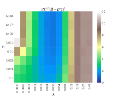
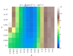
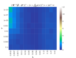
Figure 1: Heatmaps for $\|\boldsymbol{\Sigma}^{1/2}(\hat{\boldsymbol{\beta}}-{\boldsymbol{\beta}}^{*})\|^{2}$, its approximation $\|\boldsymbol{r}+({\hat{\mathsf{df}}}/{\operatorname*{tr}[\boldsymbol{V}]})\psi(\boldsymbol{r})\|^{2}/n-\|{\boldsymbol{\varepsilon}}\|^{2}/n$ and the approximation error $|\|\boldsymbol{\Sigma}^{1/2}(\hat{\boldsymbol{\beta}}-{\boldsymbol{\beta}}^{*})\|^{2}-\|\boldsymbol{r}+({\hat{\mathsf{df}}}/{\operatorname*{tr}[\boldsymbol{V}]})\psi(\boldsymbol{r})\|^{2}/n-\|{\boldsymbol{\varepsilon}}\|^{2}/n|$ for the Huber loss and Elastic-Net penalty on a grid of tuning parameters $(\lambda,\tau)$ where $\lambda\in[0.0032,0.41]$ and $\tau\in[10^{-10},0.1]$. Each cell is the average over 100 repetitions. See Section 6 for more details.

1.1 Contributions

1. The end goal of paper is to provide theoretical justification and theoretical guarantees for the criterion (2) in the high-dimensional regime where the ratio $p/n$ has a finite limit and $\boldsymbol{X}$ has anisotropic Gaussian distribution. The theoretical results will justify the approximation

   $$\big{\|}\boldsymbol{r}+\bigl{(}\hat{\mathsf{df}}/\operatorname*{tr}[\boldsymbol{V}]\bigr{)}\psi\bigl{(}\boldsymbol{r}\bigr{)}\big{\|}^{2}/n\approx\|{\boldsymbol{\varepsilon}}\|^{2}/n+\|\boldsymbol{\Sigma}^{1/2}(\widehat{{\boldsymbol{\beta}}}-{\boldsymbol{\beta}}^{*})\|^{2}.$$ (3)

Figure 1 illustrates the accuracy of (3) on simulated data. To study the criterion (2) and derive the approximation (3), we develop novel results of independent interest regarding $M$-estimators in (1):

1. The paper derives general formula for the derivatives $(\partial/\partial y_{i})\widehat{{\boldsymbol{\beta}}}$ and $(\partial/\partial x_{ij})\widehat{{\boldsymbol{\beta}}}$. This sheds light on the differentiability structure of $M$-estimators for general loss-penalty pairs: for any $\rho,g$ with $g$ strongly convex, there exists ${\widehat{\boldsymbol{A}}}\in\mathbb{R}^{p\times p}$ depending on $(\boldsymbol{y},\boldsymbol{X})$ such that for almost every $(\boldsymbol{y},\boldsymbol{X})$,

   $$(\partial/\partial y_{i})\widehat{{\boldsymbol{\beta}}}(\boldsymbol{y},\boldsymbol{X})={\widehat{\boldsymbol{A}}}\boldsymbol{X}^{\top}\boldsymbol{e}_{i}\psi^{\prime}(r_{i}),\quad(\partial/\partial x_{ij})\widehat{{\boldsymbol{\beta}}}(\boldsymbol{y},\boldsymbol{X})={\widehat{\boldsymbol{A}}}\boldsymbol{e}_{j}\psi(r_{i})-{\widehat{\boldsymbol{A}}}\boldsymbol{X}^{\top}\boldsymbol{e}_{i}\psi^{\prime}(r_{i}){\hat{\beta}}_{j},$$

   for $r_{i}=y_{i}-\boldsymbol{x}_{i}^{\top}\hat{\boldsymbol{\beta}}$, $\forall i\in[n]$,$j\in[p]$ where $\boldsymbol{e}_{j}\in\mathbb{R}^{p}$ and $\boldsymbol{e}_{i}\in\mathbb{R}^{n}$ are canonical basis vectors.

2. The paper obtains a stochastic representation for the residual $y_{i}-\boldsymbol{x}_{i}^{\top}\widehat{{\boldsymbol{\beta}}}$ for some fixed $i=1,...,n$, extending some results of [12] on unregularized $M$-estimators to penalized ones as in (1). In short, for each $i=1,...,n$ the $i$-th residual satisfies $r_{i}=y_{i}-\boldsymbol{x}_{i}^{\top}\widehat{{\boldsymbol{\beta}}}$

   $$r_{i}+(\hat{\mathsf{df}}/\operatorname*{tr}\boldsymbol{V})\psi(r_{i})\approx\varepsilon_{i}+Z_{i}\|\boldsymbol{\Sigma}^{1/2}(\widehat{{\boldsymbol{\beta}}}-{\boldsymbol{\beta}}^{*})\|$$ (4)

   where $Z_{i}\sim N(0,1)$ is independent of $\varepsilon_{i}$. This stochastic representation is the motivation for the criterion (2) as the amplitude of the normal part in the right-hand side is proportional to the out-of-sample error $\|\boldsymbol{\Sigma}^{1/2}(\widehat{{\boldsymbol{\beta}}}-{\boldsymbol{\beta}}^{*})\|$ that we wish to minimize, while the variance of the noise $\varepsilon_{i}$ does not depend on the choice of $(\rho,g)$.

Simulated data in Figure 2 confirms that the stochastic representation for the $i$-th residual $r_{i}=y_{i}-\boldsymbol{x}_{i}^{\top}\widehat{{\boldsymbol{\beta}}}$ is accurate. Our working assumption throughout the paper is the following.

Assumption 1.1.

For constants $\gamma,\mu>0$ independent of $n,p$ we have $p/n\leq\gamma$, the loss $\rho:\mathbb{R}\to\mathbb{R}$ is convex with a unique minimizer at 0, continuously differentiable and its derivative $\psi=\rho^{\prime}$ is 1-Lipschitz. The design matrix $\boldsymbol{X}$ has iid $N({\boldsymbol{0}},\boldsymbol{\Sigma})$ rows for some invertible covariance $\boldsymbol{\Sigma}$ and the noise ${\boldsymbol{\varepsilon}}$ is independent of $\boldsymbol{X}$ with continuous distribution. The penalty $g:\mathbb{R}^{p}\to\mathbb{R}$ is $\mu$-strongly convex w.r.t. $\boldsymbol{\Sigma}$ in the sense that $\boldsymbol{b}\mapsto g(\boldsymbol{b})-(\mu/2)\boldsymbol{b}^{\top}\boldsymbol{\Sigma}\boldsymbol{b}$ is convex in $\boldsymbol{b}\in\mathbb{R}^{p}$.

Throughout the paper, we consider a sequence (say, indexed by $n$) of regression problems with $p$, ${\boldsymbol{\beta}}^{*}$, $\boldsymbol{\Sigma}$ and the loss-penalty pair $(\rho,g)$ depending implicitly on $n$. For some deterministic sequence $(a_{n})$, the stochastically bounded notation $O_{P}(a_{n})$ in this context may hide constants depending on $\gamma,\mu$ only, that is, $O_{P}(a_{n})$ denotes a sequence of random variables $W_{n}$ such that for any $\varepsilon>0$ there exists $K$ depending on $(\varepsilon,\gamma,\mu)$ satisfying $\mathbb{P}(|W_{n}|\geq Ka_{n})\leq\varepsilon$.

Since Assumption 1.1 requires $p/n\leq\gamma$, the Bolzano-Weierstrass theorem lets us extract a subsequence of regression problems such that $p/n\to\gamma^{\prime}$ along this subsequence, for some constant $\gamma$. This is the asymptotic regime we have in mind throughout the paper, although our results do not require a specific limit for the ratio $p/n$. For some results, we will require the following additional assumption which is satisfied by robust loss functions and penalty that shrink towards 0.

Assumption 1.2.

The penalty is minimized at $\mathbf{0}$, that is, $g(\mathbf{0})=\min_{\boldsymbol{b}\in\mathbb{R}^{p}}g(\boldsymbol{b})$; the loss is Lipschitz as in $|\psi|\leq M$ for some constant $M$ independent of $n,p$; the signal is bounded as in $\|\boldsymbol{\Sigma}^{1/2}{\boldsymbol{\beta}}^{*}\|^{2}\leq M$.

1.2 Related works

The context of the present work is the study of $M$-estimators in the regime $\frac{p}{n}$ has a finite limit. This literature pioneered in [2, 12, 11, 18] typically describes the subtle behavior of $\widehat{{\boldsymbol{\beta}}}$ in this regime by solving a system of nonlinear equations. This system typically depends on a prior distribution for the components of ${\boldsymbol{\beta}}^{*}$, and either depends on the covariance $\boldsymbol{\Sigma}$ [8] or assume $\boldsymbol{\Sigma}=\boldsymbol{I}_{p}$ [2, 19, 7, among many others]. Solutions to the nonlinear system are a powerful tool to understand $\widehat{{\boldsymbol{\beta}}}$ in theory, e.g., to characterize the deterministic limit of $\|\boldsymbol{\Sigma}^{1/2}(\widehat{{\boldsymbol{\beta}}}-{\boldsymbol{\beta}}^{*})\|$, see e.g., the general results in [7] for the square loss and [19] for general loss-penalty pairs. However, since the system and its solution depend on unobservable quantity ($\boldsymbol{\Sigma}$ and prior on ${\boldsymbol{\beta}}^{*}$), the system solution is not directly usable for practical purposes such as parameter tuning.

The present work distinguishes itself from most of this literature as the goal is to describe the behavior of $\widehat{{\boldsymbol{\beta}}}$ using observable quantities that only depend on the data $(\boldsymbol{y},\boldsymbol{X})$ (and not unobservable ones such as $\boldsymbol{\Sigma}$ or a prior distribution on ${\boldsymbol{\beta}}^{*}$ that appear in the aforementioned nonlinear system of equations). As we will see this view lets us perform adaptive tuning of parameters in a fully adaptive manner using the criterion (2). The criterion (2) appeared in previous works for the square loss only: [1, 15] studied (2) for the Lasso with $\boldsymbol{\Sigma}=\boldsymbol{I}_{p}$ and [3, Section 3] for the square loss and general penalty (note that for the square loss $\rho(u)=u^{2}/2$, (2) reduces to $n^{2}\|\boldsymbol{r}\|^{2}/(n-\hat{\mathsf{df}})^{2}$ due to $\psi(u)=u$ and $\operatorname*{tr}[\boldsymbol{V}]=n-\hat{\mathsf{df}}$. The property $\psi(u)=u$ of the square loss hides the subtle interplay between $\boldsymbol{r},\psi(\boldsymbol{r}),\hat{\mathsf{df}}$ and $\operatorname*{tr}[\boldsymbol{V}]$ in (2) for $\rho$ different than the square loss). A criterion different from (2) is studied in [15, 3] to estimate the out-of-sample error. That criterion has the drawback to require the knowledge of $\boldsymbol{\Sigma}$, unlike (2) which is fully adaptive.

This work leverages probabilistic results on functions of standard normal random variables [5][3, §6, §7] which are consequences of Stein’s formula [17]. Consequently, the main limitation of our work is that it currently requires Gaussian design for the probabilistic results (on the other hand, the differentiability result (5) is deterministic and does not rely on any probabilistic assumption).

2 Differentiability of regularized M-estimators

The first step towards the study of the criterion (2) is to justify the almost sure existence of the derivatives of $\widehat{{\boldsymbol{\beta}}}$ that appear in (2) through the scalar scalar $\hat{\mathsf{df}}$ and the matrix $\boldsymbol{V}$ in (2). Although the criterion (2) only involves the derivatives of $\widehat{{\boldsymbol{\beta}}}(\boldsymbol{y},\boldsymbol{X})$ with respect to $\boldsymbol{y}$ for a fixed $\boldsymbol{X}$, the proof of our results rely on the interplay between the derivatives with respect to $\boldsymbol{y}$ and with respect to $\boldsymbol{X}$: this differentiability structure of $M$-estimators is the content of the following result.

Theorem 2.1.

Let Assumption 1.1 be fulfilled. For almost every $(\boldsymbol{y},\boldsymbol{X})$ the map $(\boldsymbol{y},\boldsymbol{X})\mapsto\widehat{{\boldsymbol{\beta}}}(\boldsymbol{y},\boldsymbol{X})$ is differentiable at $(\boldsymbol{y},\boldsymbol{X})$ and there exists a matrix ${\widehat{\boldsymbol{A}}}\in\mathbb{R}^{p\times p}$ with $\|\boldsymbol{\Sigma}^{1/2}{\widehat{\boldsymbol{A}}}\boldsymbol{\Sigma}^{1/2}\|_{op}\leq(n\mu)^{-1}$ s.t.

$$\begin{split}(\partial/\partial y_{i})\widehat{{\boldsymbol{\beta}}}(\boldsymbol{y},\boldsymbol{X})&={\widehat{\boldsymbol{A}}}\boldsymbol{X}^{\top}\boldsymbol{e}_{i}\psi^{\prime}(r_{i}),\\ (\partial/\partial x_{ij})\widehat{{\boldsymbol{\beta}}}(\boldsymbol{y},\boldsymbol{X})&={\widehat{\boldsymbol{A}}}\boldsymbol{e}_{j}\psi(r_{i})-{\widehat{\boldsymbol{A}}}\boldsymbol{X}^{\top}\boldsymbol{e}_{i}\psi^{\prime}(r_{i}){\hat{\beta}}_{j},\end{split}\qquad\text{ where }r_{i}=y_{i}-\boldsymbol{x}_{i}^{\top}\hat{\boldsymbol{\beta}},$$ (5)

$\boldsymbol{e}_{i}\in\mathbb{R}^{n},\boldsymbol{e}_{j}\in\mathbb{R}^{p}$ are canonical basis vectors , $\psi:=\rho^{\prime}$ and $\psi^{\prime}$ denote the derivatives. Furthermore,

$$\hat{\mathsf{df}}=\operatorname*{tr}[\boldsymbol{X}(\partial/\partial\boldsymbol{y})\hat{\boldsymbol{\beta}}] =\operatorname*{tr}[\boldsymbol{X}{\widehat{\boldsymbol{A}}}\boldsymbol{X}\operatorname*{diag}\{\psi^{\prime}(\boldsymbol{r})\}],$$ (6)

$$\boldsymbol{V}=\operatorname*{diag}\{\psi^{\prime}(\boldsymbol{r})\}(\boldsymbol{I}_{n}-\boldsymbol{X}(\partial/\partial\boldsymbol{y})\widehat{{\boldsymbol{\beta}}}) =\operatorname*{diag}\{\psi^{\prime}(\boldsymbol{r})\}-\operatorname*{diag}\{\psi^{\prime}(\boldsymbol{r})\}\boldsymbol{X}{\widehat{\boldsymbol{A}}}\boldsymbol{X}\operatorname*{diag}\{\psi^{\prime}(\boldsymbol{r})\}.$$ (7)

satisfy $0\leq\hat{\mathsf{df}}\leq n$ and $0\leq\operatorname*{tr}[\boldsymbol{V}]\leq n$.

Since the same matrix ${\widehat{\boldsymbol{A}}}$ appears in both the derivatives with respect to $y_{i}$ and to $x_{ij}$, (5) provides relationship between $(\partial/\partial y_{i})\widehat{{\boldsymbol{\beta}}}$ and $(\partial/\partial x_{ij})\widehat{{\boldsymbol{\beta}}}$, for instance $(\partial/\partial x_{ij})\widehat{{\boldsymbol{\beta}}}={\widehat{\boldsymbol{A}}}\boldsymbol{e}_{j}\psi(r_{i})-{\hat{\beta}}_{j}(\partial/\partial y_{i})\widehat{{\boldsymbol{\beta}}}$. Although the matrix ${\widehat{\boldsymbol{A}}}$ is not explicit for arbitrary loss-penalty pair, closed-form expressions are available for particular examples such as the Elastic-Net penalty as discussed in Section 6.

Remark 2.1.

For the square loss $\rho(u)=u^{2}/2$, the differentiability formulae (5) reduce to

$$(\partial/\partial y_{l})\widehat{{\boldsymbol{\beta}}}(\boldsymbol{y},\boldsymbol{X})={\widehat{\boldsymbol{A}}}\boldsymbol{X}^{\top}\boldsymbol{e}_{l},\qquad(\partial/\partial x_{ij})\widehat{{\boldsymbol{\beta}}}(\boldsymbol{y},\boldsymbol{X})={\widehat{\boldsymbol{A}}}\boldsymbol{e}_{j}(y_{i}-\boldsymbol{x}_{i}^{\top}\widehat{{\boldsymbol{\beta}}})-{\widehat{\boldsymbol{A}}}\boldsymbol{X}^{\top}\boldsymbol{e}_{i}{\hat{\beta}}_{j}$$

for most every $(\boldsymbol{y},\boldsymbol{X})$ and some matrix ${\widehat{\boldsymbol{A}}}\in\mathbb{R}^{p\times p}$ depending on $(\boldsymbol{y},\boldsymbol{X})$, since in this case $\psi^{\prime}=1$.

In the simple case where $g$ is twice continuously differentiable, (5) follows [5] with

$${\widehat{\boldsymbol{A}}}=\bigl{(}\boldsymbol{X}^{\top}\operatorname*{diag}\{\psi^{\prime}(\boldsymbol{r})\}\boldsymbol{X}+n\nabla^{2}g(\widehat{{\boldsymbol{\beta}}})\bigr{)}^{-1}$$ (8)

by differentiating the KKT conditions $\boldsymbol{X}^{\top}\psi(\boldsymbol{y}-\boldsymbol{X}\widehat{{\boldsymbol{\beta}}})=n\nabla g(\widehat{{\boldsymbol{\beta}}})$. To illustrate why this is true, provided that $\widehat{{\boldsymbol{\beta}}}(\boldsymbol{y},\boldsymbol{X})$ is differentiable, if $(\boldsymbol{y}(t),\boldsymbol{X}(t))$ are smooth perturbations of $(\boldsymbol{y},\boldsymbol{X})$ with $(\boldsymbol{y}(0),\boldsymbol{X}(0))=(\boldsymbol{y},\boldsymbol{X})$ and $\frac{d}{dt}(\boldsymbol{y}(t),\boldsymbol{X}(t))|_{t=0}=(\dot{\boldsymbol{y}},\dot{\boldsymbol{X}})$, differentiation of $\boldsymbol{X}(t){}^{\top}\psi(\boldsymbol{y}(t)-\boldsymbol{X}(t)\widehat{{\boldsymbol{\beta}}}(\boldsymbol{y}(t),\boldsymbol{X}(t)))=n\nabla g(\widehat{{\boldsymbol{\beta}}}(\boldsymbol{y}(t),\boldsymbol{X}(t)))$ at $t=0$ and the chain rule yields

$$\dot{\boldsymbol{X}}{}^{\top}\psi(\boldsymbol{r})-\boldsymbol{X}^{\top}\operatorname*{diag}\{\psi^{\prime}(\boldsymbol{r})\}(\dot{\boldsymbol{y}}-\dot{\boldsymbol{X}}\widehat{{\boldsymbol{\beta}}}(\boldsymbol{y},\boldsymbol{X}))={\widehat{\boldsymbol{A}}}{}^{-1}\tfrac{d}{dt}\widehat{{\boldsymbol{\beta}}}(\boldsymbol{y}(t),\boldsymbol{X}(t))\big{|}_{t=0}$$

with ${\widehat{\boldsymbol{A}}}$ in (8). This gives (5) if the penalty $g$ is twice-differentiable. Theorem 2.1 reveals that for arbitrary convex penalty functions including non-differentiable ones, the differentiability structure (5) always holds, as in the case of twice differentiable penalty $g$, even for penalty functions such as $g(\boldsymbol{b})=\mu\|\boldsymbol{b}\|^{2}/2+\lambda\|\text{mat}(\boldsymbol{b})\|_{\rm nuc}$ where $\text{mat}:\mathbb{R}^{p}\to\mathbb{R}^{d_{1}\times d_{2}}$ is a linear isomorphism to the space of $d_{1}\times d_{2}$ matrices and $\|\cdot\|_{\rm nuc}$ is the nuclear norm: in this case by Theorem 2.1 there exists a matrix ${\widehat{\boldsymbol{A}}}\in\mathbb{R}^{p\times p}$ such that (5) holds although no closed-form expression for ${\widehat{\boldsymbol{A}}}$ is known.

The representation (5) is a powerful tool as it provides explicit derivatives of quantities of interest such as $\boldsymbol{r}=\boldsymbol{y}-\boldsymbol{X}\widehat{{\boldsymbol{\beta}}}$, $\|\psi(\boldsymbol{r})\|^{2}$ or $\|\boldsymbol{\Sigma}^{1/2}(\widehat{{\boldsymbol{\beta}}}-{\boldsymbol{\beta}}^{*})\|^{2}$. These explicit derivatives can then be used in probabilistic identities and inequalities that involve derivatives, for instance Stein’s formulae [17], the Gaussian Poincaré inequalty [6, Theorem 3.20], or normal approximations [9, 5].

Remark 2.2.

Similar derivative formulae hold if an intercept is included in the minimization, as in

$$\bigl{(}{\hat{\beta}}_{0}(\boldsymbol{y},\boldsymbol{X}),~{}\widehat{{\boldsymbol{\beta}}}(\boldsymbol{y},\boldsymbol{X})\bigr{)}=\operatorname*{argmin}_{b_{0}\in\mathbb{R},\boldsymbol{b}\in\mathbb{R}^{p}}\frac{1}{n}\sum_{i=1}^{n}\rho(y_{i}-b_{0}-\boldsymbol{x}_{i}^{\top}\boldsymbol{b})+g(\boldsymbol{b})$$ (9)

Let Assumption 1.1 be fulfilled, and assume further $\|\psi^{\prime}(\boldsymbol{r})\|_{2}>0$ with $\boldsymbol{r}:=\boldsymbol{y}-{\boldsymbol{1}}_{n}\hat{\beta}_{0}-\boldsymbol{x}_{i}^{\top}\widehat{{\boldsymbol{\beta}}}$ where ${\boldsymbol{1}}_{n}=(1,...,1)^{\top}\in\mathbb{R}^{n}$. For almost every $(\boldsymbol{y},\boldsymbol{X})$ the map $(\boldsymbol{y},\boldsymbol{X})\mapsto\widehat{{\boldsymbol{\beta}}}(\boldsymbol{y},\boldsymbol{X})$ is differentiable at $(\boldsymbol{y},\boldsymbol{X})$, and there exists ${\widehat{\boldsymbol{A}}}\in\mathbb{R}^{p\times p}$ depending on $(\boldsymbol{y},\boldsymbol{X})$ with $\|\boldsymbol{\Sigma}^{1/2}{\widehat{\boldsymbol{A}}}\boldsymbol{\Sigma}^{1/2}\|_{op}\leq(n\mu)^{-1}$ such that

$$(\partial/\partial y_{i})\widehat{{\boldsymbol{\beta}}}(\boldsymbol{y},\boldsymbol{X})={\widehat{\boldsymbol{A}}}\boldsymbol{X}^{\top}\boldsymbol{\Psi}^{\prime}\boldsymbol{e}_{i},\quad(\partial/\partial x_{ij})\widehat{{\boldsymbol{\beta}}}(\boldsymbol{y},\boldsymbol{X})={\widehat{\boldsymbol{A}}}\boldsymbol{e}_{j}\psi(r_{i})-{\widehat{\boldsymbol{A}}}\boldsymbol{X}^{\top}\boldsymbol{\Psi}^{\prime}\boldsymbol{e}_{i}{\hat{\beta}}_{j},$$ (10)

where $\boldsymbol{e}_{i}\in\mathbb{R}^{n},\boldsymbol{e}_{j}\in\mathbb{R}^{p}$ are canonical basis vectors, $\psi=\rho^{\prime}$ and $\boldsymbol{\Psi}^{\prime}:=\operatorname*{diag}\{\psi^{\prime}(\boldsymbol{r})\}-\psi^{\prime}(\boldsymbol{r})\psi^{\prime}(\boldsymbol{r})^{\top}/\sum_{i\in[n]}\psi^{\prime}(r_{i})$.

3 Distribution of individual residuals

We now turn to the distribution of a single residual $r_{i}=y_{i}-\boldsymbol{x}_{i}^{\top}\widehat{{\boldsymbol{\beta}}}$ for some fixed observation $i\in\{1,...,n\}$ (for instance, fix $i=1$). By leveraging the differentiability structure (5) and the normal approximation from [5], the following result provides a clear picture of the distribution of $r_{i}$.

Theorem 3.1.

Let Assumption 1.1 be fulfilled and let ${\widehat{\boldsymbol{A}}}\in\mathbb{R}^{p\times p}$ be given by Theorem 2.1. Then for every $i=1,...,n$ there exists $Z_{i}\sim N(0,1)$ such that

$$\Big{|}\Bigl{(}r_{i}+\operatorname*{tr}[\boldsymbol{\Sigma}{\widehat{\boldsymbol{A}}}]\psi(r_{i})\Bigr{)}-\Bigl{(}\varepsilon_{i}+\|\boldsymbol{\Sigma}^{1/2}(\widehat{{\boldsymbol{\beta}}}-{\boldsymbol{\beta}}^{*})\|Z_{i}\Bigr{)}\Big{|}\leq O_{P}(n^{-1/4})(|\psi(\varepsilon_{i})|+\|\boldsymbol{\Sigma}^{1/2}(\widehat{{\boldsymbol{\beta}}}-{\boldsymbol{\beta}}^{*})\|)$$ (11)

Furthermore, if $\varepsilon_{i}$ has a fixed distribution $F$, there exists a bivariate variable $(\tilde{\varepsilon}_{i}^{n},\tilde{Z}_{i}^{n})$ converging in distribution to the product measure $F\otimes N(0,1)$ such that

$$r_{i}+\operatorname*{tr}[\boldsymbol{\Sigma}{\widehat{\boldsymbol{A}}}]\psi(r_{i})=\tilde{\varepsilon}_{i}^{n}+\|\boldsymbol{\Sigma}^{1/2}(\widehat{{\boldsymbol{\beta}}}-{\boldsymbol{\beta}}^{*})\|\tilde{Z}_{i}^{n}.$$ (12)

If $\varepsilon_{i}$ has a fixed distribution $F$ and Assumption 1.2 holds then $|\psi(\varepsilon_{i})|+\|\boldsymbol{\Sigma}^{1/2}(\widehat{{\boldsymbol{\beta}}}-{\boldsymbol{\beta}}^{*})\|=O_{P}(1)$.

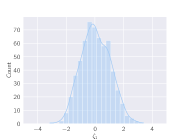
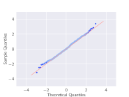
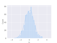
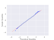
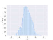
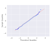
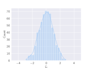
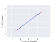
Figure 2: Histogram and QQ-plot for $\zeta_{1}$ in (13) under Huber Elastic-Net regression for different choices of tuning parameters $(\lambda,\tau)$. Left Top: $(0.036,10^{-10})$, Right Top: $(0.054,0.01)$, Left Bottom: $(0.036,0.01)$, Right Bottom: $(0.024,0.1)$. Each figure contains 600 data points generated with anisotropic design matrix and iid $\varepsilon_{i}$ from the $t$-distribution with 2 degrees of freedom. A detailed setup is provided in Section 6.

Theorem 3.1 is a formal statement regarding the informal normal approximation

$$\zeta_{i}:=\frac{r_{i}+\operatorname*{tr}[\boldsymbol{\Sigma}{\widehat{\boldsymbol{A}}}]\psi(r_{i})-\varepsilon_{i}}{\|\boldsymbol{\Sigma}^{1/2}(\hat{\boldsymbol{\beta}}-{\boldsymbol{\beta}}^{*})\|}\approx N(0,1).$$ (13)

Simulations in Figure 2 confirm the normality of $\zeta_{i}$ for the Huber loss with Elastic-Net penalty and four combinations of tuning parameters. For the square loss $\rho(u)=u^{2}/2$, because $\psi(u)=u$, asymptotic normality of the residuals hold in the following form.

Theorem 3.2.

Let Assumption 1.1 hold with $\rho(u)=u^{2}/2$ and ${\boldsymbol{\varepsilon}}\sim N(\mathbf{0},\sigma^{2}\boldsymbol{I}_{n})$. Then for $i=1$,

$$(\sigma^{2}+\|\boldsymbol{\Sigma}^{1/2}(\widehat{{\boldsymbol{\beta}}}-{\boldsymbol{\beta}}^{*})\|^{2})^{-1/2}(1+\operatorname*{tr}[\boldsymbol{\Sigma}{\widehat{\boldsymbol{A}}}])(y_{i}-\boldsymbol{x}_{i}^{\top}\widehat{{\boldsymbol{\beta}}})\to^{d}N(0,1)\qquad\text{ as }n\to+\infty.$$ (14)

It is informative to provide a sketch of the proof of Theorem 3.1 to explain the appearance of $\psi(r_{i})$ and $\operatorname*{tr}[\boldsymbol{\Sigma}{\widehat{\boldsymbol{A}}}]$ in the normal approximation results (11) and (13). A variant of the normal approximation of [5] proved in the supplement states that for a differentiable function $\mathbf{f}:\mathbb{R}^{q}\to\mathbb{R}^{q}\setminus\{\mathbf{0}\}$ and $\boldsymbol{z}\sim N({\boldsymbol{0}},\boldsymbol{I}_{q})$, there exists $Z\sim N(0,1)$ such hat

$$\mathbb{E}\Bigl{[}\Bigl{|}\frac{\mathbf{f}(\boldsymbol{z})^{\top}\boldsymbol{z}-\sum_{k=1}^{q}(\partial/\partial z_{k})f_{k}(\boldsymbol{z})}{\|\mathbf{f}(\boldsymbol{z})\|}-Z\Bigr{|}^{2}\Bigr{]}\leq\C\mathbb{E}\Bigl{[}\frac{\sum_{k=1}^{q}\|(\partial/\partial z_{k})\mathbf{f}(\boldsymbol{z})\|^{2}}{\|\mathbf{f}(\boldsymbol{z})\|^{2}}\Bigr{]}.$$ (15)

Some technical hurdles aside, the proof sketch is the following: Apply the previous display to $q=p$, $\boldsymbol{z}=\boldsymbol{\Sigma}^{-1/2}\boldsymbol{x}_{i}$ conditionally on $({\boldsymbol{\varepsilon}},(\boldsymbol{x}_{l})_{l\in[n]\setminus\{i\}})$ and to $\mathbf{f}(\boldsymbol{z})=\boldsymbol{\Sigma}^{1/2}(\widehat{{\boldsymbol{\beta}}}-{\boldsymbol{\beta}}^{*})$ in the simple case where ${\boldsymbol{\beta}}^{*}=0$ (this amounts to performing a change of variable by translation of $\widehat{{\boldsymbol{\beta}}}$ to $\widehat{{\boldsymbol{\beta}}}-{\boldsymbol{\beta}}^{*}$). Then the right-hand side of the previous display is negligible in probability compared to $Z$, and in the left-hand side $\mathbf{f}(\boldsymbol{z})^{\top}\boldsymbol{z}=\boldsymbol{x}_{i}^{\top}(\widehat{{\boldsymbol{\beta}}}-{\boldsymbol{\beta}}^{*})$ and $\sum_{k=1}^{q}(\partial/\partial z_{k})f_{k}(\boldsymbol{z})\approx\operatorname*{tr}[\boldsymbol{\Sigma}{\widehat{\boldsymbol{A}}}]\psi(r_{i})$ as the second term in (5) is negligible. This completes the sketch of the proof of (13).

Proximal operator representation.

From the above asymptotic normality results, a stochastic representation for the $i$-th residual $r_{i}=y_{i}-\boldsymbol{x}_{i}^{\top}\smash{\widehat{{\boldsymbol{\beta}}}}$ can be obtained as follows: With $\operatorname*{prox}[t\rho](u)$ the proximal operator of $x\mapsto t\rho(x)$ defined as the unique solution $z\in\mathbb{R}$ of equation $z+t\psi(z)=u$,

$$r_{i}=y_{i}-\boldsymbol{x}_{i}^{\top}\widehat{{\boldsymbol{\beta}}}=\operatorname*{prox}[\hat{t}\rho]\bigl{(}\tilde{\varepsilon}_{i}^{n}+\|\boldsymbol{\Sigma}^{1/2}(\widehat{{\boldsymbol{\beta}}}-{\boldsymbol{\beta}}^{*})\|\tilde{Z}_{i}^{n}\bigr{)}\qquad\text{ with }\hat{t}=\operatorname*{tr}[\boldsymbol{\Sigma}{\widehat{\boldsymbol{A}}}]$$

where $(\tilde{\varepsilon}_{i}^{n},\tilde{Z}_{i}^{n})$ converges in distribution to product measure $F\otimes N(0,1)$ where $F$ is the law of $\varepsilon_{i}$.

4 A proxy of the out-of-sample error if $\boldsymbol{\Sigma}$ is known

The approximations of the previous sections for $r_{i}+\operatorname*{tr}[\boldsymbol{\Sigma}{\widehat{\boldsymbol{A}}}]\psi(r_{i})$ and the fact that $\varepsilon_{i}$ is independent of $Z_{i}\sim N(0,1)$ in (11) suggest that $(r_{i}+\operatorname*{tr}[\boldsymbol{\Sigma}{\widehat{\boldsymbol{A}}}]\psi(r_{i}))^{2}\approx\varepsilon_{i}^{2}+\|\boldsymbol{\Sigma}^{1/2}(\widehat{{\boldsymbol{\beta}}}-{\boldsymbol{\beta}}^{*})\|^{2}Z_{i}^{2}$; and averaging over $\{1,...,n\}$ one can hope for the approximation $\|\boldsymbol{r}+\operatorname*{tr}[\boldsymbol{\Sigma}{\widehat{\boldsymbol{A}}}]\psi(\boldsymbol{r})\|^{2}/n\approx\|{\boldsymbol{\varepsilon}}\|^{2}/n+\|\boldsymbol{\Sigma}^{1/2}(\widehat{{\boldsymbol{\beta}}}-{\boldsymbol{\beta}}^{*})\|^{2}$. The following result makes this heuristic precise.

Theorem 4.1.

Let Assumption 1.1 be fulfilled and ${\widehat{\boldsymbol{A}}}$ be given by Theorem 2.1. Then

$$\|\boldsymbol{\Sigma}^{1/2}(\widehat{{\boldsymbol{\beta}}}-{\boldsymbol{\beta}}^{*})\|^{2}+\|{\boldsymbol{\varepsilon}}\|^{2}/n=\big{\|}\boldsymbol{r}+\operatorname*{tr}[\boldsymbol{\Sigma}{\widehat{\boldsymbol{A}}}]\psi(\boldsymbol{r})\big{\|}^{2}/n+O_{P}(n^{-1/2})\operatorname{Rem},$$

where $\operatorname{Rem}:=\|\boldsymbol{\Sigma}^{1/2}(\hat{\boldsymbol{\beta}}-{\boldsymbol{\beta}}^{*})\|^{2}+\frac{1}{n}\|\psi(\boldsymbol{r})\|^{2}+(\|\boldsymbol{\Sigma}^{1/2}(\hat{\boldsymbol{\beta}}-{\boldsymbol{\beta}}^{*})\|^{2}+\frac{1}{n}\|\psi(\boldsymbol{r})\|^{2})^{1/2}\|\frac{1}{\sqrt{n}}{\boldsymbol{\varepsilon}}\|$. Thus

$$\|\boldsymbol{\Sigma}^{1/2}(\widehat{{\boldsymbol{\beta}}}-{\boldsymbol{\beta}}^{*})\|^{2}+\|{\boldsymbol{\varepsilon}}\|^{2}/n=(1+O_{P}(n^{-1/2}))\big{\|}\boldsymbol{r}+\operatorname*{tr}[\boldsymbol{\Sigma}{\widehat{\boldsymbol{A}}}]\psi(\boldsymbol{r})\big{\|}^{2}/n.$$

Theorem 4.1 provides a first candidate, $\big{\|}\boldsymbol{r}+\operatorname*{tr}[\boldsymbol{\Sigma}{\widehat{\boldsymbol{A}}}]\psi(\boldsymbol{r})\big{\|}^{2}/n$ to estimate

$$\|\boldsymbol{\Sigma}^{1/2}(\widehat{{\boldsymbol{\beta}}}-{\boldsymbol{\beta}}^{*})\|^{2}+\|{\boldsymbol{\varepsilon}}\|^{2}/n.$$ (16)

Estimation of (16) is useful as $\|{\boldsymbol{\varepsilon}}\|^{2}/n$ is independent of the choice of the estimator $\widehat{{\boldsymbol{\beta}}}$ and in particular independent of the chosen loss-penalty pair in (1). Given two or more estimators (1), choosing the one with smallest $\big{\|}\boldsymbol{r}+\operatorname*{tr}[\boldsymbol{\Sigma}{\widehat{\boldsymbol{A}}}]\psi(\boldsymbol{r})\big{\|}^{2}$ is thus a good proxy for minimizing the out-of-sample error.

Corollary 4.2.

Let $\widehat{{\boldsymbol{\beta}}},\widetilde{{\boldsymbol{\beta}}}$ be two $M$-estimators (1) Assumption 1.1 with loss-penalty pair $(\rho,g)$ and $(\tilde{\rho},\tilde{g})$ respectively. Assume that both satisfy Assumption 1.1 and let $\psi=\rho^{\prime}$ and $\tilde{\psi}=\tilde{\rho}^{\prime}$. Let $\boldsymbol{r}=\boldsymbol{y}-\boldsymbol{X}\widehat{{\boldsymbol{\beta}}},{\widetilde{\boldsymbol{r}}}=\boldsymbol{y}-\boldsymbol{X}\widetilde{{\boldsymbol{\beta}}}$ be the residuals, ${\widehat{\boldsymbol{A}}},{\widetilde{\boldsymbol{A}}}$ be the corresponding matrices of size $p\times p$ given by Theorem 2.1. Further assume that both estimators satisfy Assumption 1.2 and that ${\boldsymbol{\varepsilon}}$ has iid coordinates independent with $\mathbb{E}[|\varepsilon_{i}|^{1+q}]\leq M$ for constants $q\in(0,1),M>0$ independent of $n,p$. Let $\Omega=\{\|\boldsymbol{X}\boldsymbol{\Sigma}^{-1/2}\|_{op}\leq 2\sqrt{n}+\sqrt{p}\}\cap\{\|{\boldsymbol{\varepsilon}}\|^{2}\leq n^{2/(1+q)}\}$. Then for any $\eta>0$ independent of $n,p$ there exists $C(\gamma,\mu,\eta,q,M)>0$ depending only on $\{\gamma,\mu,\eta,q,M\}$ such that

$$\mathbb{P}\Bigl{(}\|\boldsymbol{\Sigma}^{1/2}(\widehat{{\boldsymbol{\beta}}}-{\boldsymbol{\beta}}^{*})\|^{2}-\|\boldsymbol{\Sigma}^{1/2}(\widetilde{{\boldsymbol{\beta}}}-{\boldsymbol{\beta}}^{*})\|^{2}>\eta,~{}~{}\|\boldsymbol{r}+\operatorname*{tr}[\boldsymbol{\Sigma}{\widehat{\boldsymbol{A}}}]\psi(\boldsymbol{r})\|^{2}\leq\|{\widetilde{\boldsymbol{r}}}+\operatorname*{tr}[\boldsymbol{\Sigma}{\widetilde{\boldsymbol{A}}}]\tilde{\psi}({\widetilde{\boldsymbol{r}}})\|^{2}\Bigr{)}\\ \leq C(\gamma,\mu,\eta,q,M)n^{-q/(1+q)}+\mathbb{P}(\Omega^{c})\to 0.$$

Provided that the noise random variables $\varepsilon_{i}$ have at least $1+q$ moments, Corollary 4.2 implies that with probability approaching one given two $M$-estimators $\widehat{{\boldsymbol{\beta}}}$ and $\widetilde{{\boldsymbol{\beta}}}$, choosing the estimator corresponding to the smallest criteria among $\|\boldsymbol{r}+\operatorname*{tr}[\boldsymbol{\Sigma}{\widehat{\boldsymbol{A}}}]\boldsymbol{r}\|^{2}$ and $\|{\widetilde{\boldsymbol{r}}}+\operatorname*{tr}[\boldsymbol{\Sigma}{\widetilde{\boldsymbol{A}}}]{\widetilde{\boldsymbol{r}}}\|^{2}$ leads to the smallest out-of-sample error, up to any small constant $\eta>0$. This allows noise random variables $\varepsilon_{i}$ with infinite variance. A similar result can be obtained to select among $K$ different $M$-estimators (1).

Corollary 4.3.

As in Corollary 4.2, assume $\mathbb{E}[|\varepsilon_{i}|^{1+q}]\leq M$ and let $\widehat{{\boldsymbol{\beta}}}_{1},...,\widehat{{\boldsymbol{\beta}}}_{K}$ be $M$-estimators of the form (1) with loss-penalty pair $(\rho_{k},g_{k})$ satisfying Assumptions 1.1 and 1.2. For each $k=1,...,K$, let $\boldsymbol{r}_{k}=\boldsymbol{y}-\boldsymbol{X}\widehat{{\boldsymbol{\beta}}}_{k}$ be the residuals and ${\widehat{\boldsymbol{A}}}_{k}$ be the corresponding matrix of size $p\times p$ from Theorem 2.1. Let $\hat{k}\in\operatorname*{argmin}_{k=1,...,K}\|\boldsymbol{r}_{k}+\operatorname*{tr}[\boldsymbol{\Sigma}{\widehat{\boldsymbol{A}}}_{k}]\psi_{k}(\boldsymbol{r}_{k})\|$ where $\psi_{k}=\rho_{k}^{\prime}$. Then if $(\gamma,\mu,\eta,q,M)$ are constants independent of $n,p$

$$\textstyle\mathbb{P}\bigl{(}\|\boldsymbol{\Sigma}^{1/2}(\widehat{{\boldsymbol{\beta}}}_{\hat{k}}-{\boldsymbol{\beta}}^{*})\|^{2}>\min_{k=1,...,K}\|\boldsymbol{\Sigma}^{1/2}(\widehat{{\boldsymbol{\beta}}}_{k}-{\boldsymbol{\beta}}^{*})\|^{2}+\eta\bigr{)}\to 0\qquad\text{ if }K=o(n^{q/(1+q)}).$$

Given $K$ different loss-penalty pairs and the corresponding $M$-estimators in (1), minimizing the criterion $\|\boldsymbol{r}+\operatorname*{tr}[\boldsymbol{\Sigma}{\widehat{\boldsymbol{A}}}]\boldsymbol{r}\|$ thus provably selects a loss-penalty pair that leads to an optimal out-of-sample error, up to an arbitrary small constant $\eta>0$ independent of $n,p$. The requirement $K=o(n^{q/(1+q)})$ means that the cardinality of the collection of $M$-estimators to select from should grow more slowly than a power of $n$. This is typically satisfied for default tuning parameter grids in popular libraries (e.g., sklearn.linear_model.Lasso [16]) with tuning parameters evenly spaced in a log-scale that consequently have cardinality logarithmic in the parameter range. The major drawback of the criterion $\|\boldsymbol{r}+\operatorname*{tr}[\boldsymbol{\Sigma}{\widehat{\boldsymbol{A}}}]\boldsymbol{r}\|$ is the dependence through $\operatorname*{tr}[\boldsymbol{\Sigma}{\widehat{\boldsymbol{A}}}]$ on the covariance $\boldsymbol{\Sigma}$ of the design, which is typically unknown. The next section introduces an estimator of $\operatorname*{tr}[\boldsymbol{\Sigma}{\widehat{\boldsymbol{A}}}]$ that does not require the knowledge of $\boldsymbol{\Sigma}$.

5 Degrees of freedom and estimating $\operatorname*{tr}[\boldsymbol{\Sigma}{\widehat{\boldsymbol{A}}}]$ without the knowledge of $\boldsymbol{\Sigma}$

This section focuses on estimating $\operatorname*{tr}[\boldsymbol{\Sigma}{\widehat{\boldsymbol{A}}}]$. The matrix ${\widehat{\boldsymbol{A}}}$ from Theorem 2.1 can be estimated from the data $(\boldsymbol{y},\boldsymbol{X})$ in the sense that ${\widehat{\boldsymbol{A}}}$ is a measurable function of $(\boldsymbol{y},\boldsymbol{X})$ (thanks to the observation that derivatives are limits, and limits of measurable functions are again measurable). The difficulty is thus to estimate $\operatorname*{tr}[\boldsymbol{\Sigma}{\widehat{\boldsymbol{A}}}]$ without the knowledge of $\boldsymbol{\Sigma}$. To illustrate this difficulty, consider Ridge regression with square loss $\rho(u)=u^{2}/2$ and penalty $g(\boldsymbol{b})=\tau\|\boldsymbol{b}\|^{2}/2$. Then $\widehat{{\boldsymbol{\beta}}}(\boldsymbol{y},\boldsymbol{X})=(\boldsymbol{X}^{\top}\boldsymbol{X}+\tau n\boldsymbol{I}_{p})^{-1}\boldsymbol{X}^{\top}\boldsymbol{y}$ and ${\widehat{\boldsymbol{A}}}$ in Theorem 2.1 is given explicitly by ${\widehat{\boldsymbol{A}}}=(\boldsymbol{X}^{\top}\boldsymbol{X}+\tau n\boldsymbol{I}_{p})^{-1}$ and

$$\operatorname*{tr}[\boldsymbol{\Sigma}{\widehat{\boldsymbol{A}}}]=\operatorname*{tr}[(\boldsymbol{G}^{\top}\boldsymbol{G}+n\tau\boldsymbol{\Sigma}^{-1})^{-1}],\qquad\text{ where }\boldsymbol{G}=\boldsymbol{X}\boldsymbol{\Sigma}^{-1/2}.$$

Above, $\boldsymbol{G}$ is a random matrix with iid $N(0,1)$ entries the value of $\operatorname*{tr}[\boldsymbol{\Sigma}{\widehat{\boldsymbol{A}}}]$ is highly dependent on the spectrum of $\boldsymbol{\Sigma}^{-1}$. In this particular case, the limit of $\operatorname*{tr}[(\boldsymbol{G}^{\top}\boldsymbol{G}+n\tau\boldsymbol{\Sigma}^{-1})^{-1}]$ can be obtained using random matrix theory [14] as the limiting behavior of the Stieltjes transform of $\boldsymbol{G}^{\top}\boldsymbol{G}/n+\tau\boldsymbol{\Sigma}^{-1}$ and its spectral distribution is known; however the limit of the spetral distribution depends on the spectrum of $\tau\boldsymbol{\Sigma}^{-1}$. This is not desirable here as we wish to construct estimators that require no knowledge on $\boldsymbol{\Sigma}$. For more involved loss-penalty pairs such as the Elastic-Net in Example 6.1, such random matrix theory results do not apply as $\operatorname*{tr}[\boldsymbol{\Sigma}{\widehat{\boldsymbol{A}}}]$ depends on the random support of $\widehat{{\boldsymbol{\beta}}}$.

Instead, we do not rely on known random matrix theory results. With the matrix ${\widehat{\boldsymbol{A}}}\in\mathbb{R}^{p\times p}$ given by Theorem 2.1, our proposal to estimate $\operatorname*{tr}[\boldsymbol{\Sigma}{\widehat{\boldsymbol{A}}}]$ is the ratio $\hat{\mathsf{df}}/\operatorname*{tr}[\boldsymbol{V}]$ with $\hat{\mathsf{df}}$ and $\boldsymbol{V}$ in (6)-(7). Both the scalar $\hat{\mathsf{df}}$ and the matrix $\boldsymbol{V}\in\mathbb{R}^{n\times n}$ are observable; in particular they do not depend on $\boldsymbol{\Sigma}$.

Theorem 5.1.

Let Assumption 1.1 be fulfilled and ${\widehat{\boldsymbol{A}}}$ be given by Theorem 2.1. Then

$$\mathbb{E}[|\operatorname*{tr}[\boldsymbol{\Sigma}{\widehat{\boldsymbol{A}}}]\operatorname*{tr}[\boldsymbol{V}]/n-\hat{\mathsf{df}}/n|]\leq\C(\gamma,\mu)n^{-1/2}.$$ (17)

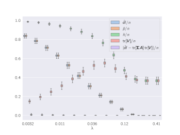
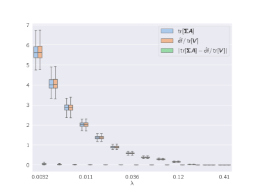
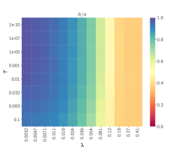
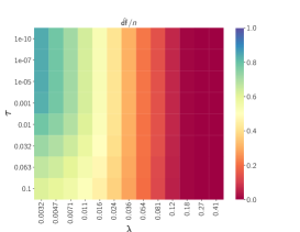
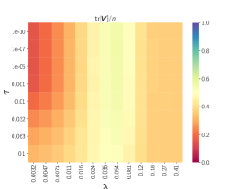
Figure 3: Above: Boxplots for $\hat{\mathsf{df}},\hat{p},\hat{n},\operatorname*{tr}[\boldsymbol{V}],\operatorname*{tr}[\boldsymbol{\Sigma}{\widehat{\boldsymbol{A}}}]$ and $|\operatorname*{tr}[\boldsymbol{\Sigma}{\widehat{\boldsymbol{A}}}]-\hat{\mathsf{df}}/\operatorname*{tr}[\boldsymbol{V}]|$ in Huber Elastic-Net regression with $\tau=10^{-10}$ and $\lambda\in[0.0032,0.41].$ Each box contains 200 data points. Below: heatmaps for $\hat{\mathsf{df}}/n$, $\operatorname*{tr}[\boldsymbol{V}]/n$ and $\hat{n}/n=\sum_{i=1}^{n}\psi^{\prime}(r_{i})/n$ under the simulation setup in Figure 1. The detailed simulation setup is given in Section 6.

Simulations in Figures 3 and 1 confirm that the approximation $\operatorname*{tr}[\boldsymbol{\Sigma}{\widehat{\boldsymbol{A}}}]\approx\hat{\mathsf{df}}/\operatorname*{tr}[\boldsymbol{V}]$ is accurate for the Huber loss with Elastic-Net penalty. For the square loss, $\psi^{\prime}=1$ and $\operatorname*{tr}[\boldsymbol{V}]=n-\hat{\mathsf{df}}$ so that (17) becomes $\mathbb{E}|(1-\hat{\mathsf{df}}/n)(1+\operatorname*{tr}[\boldsymbol{\Sigma}{\widehat{\boldsymbol{A}}}])-1|\leq\C(\gamma,\mu)n^{-1/2}$ and the following result holds.

Corollary 5.2.

Let Assumption 1.1 be fulfilled with $\rho(u)=u^{2}/2$ and ${\boldsymbol{\varepsilon}}\sim N(\mathbf{0},\sigma^{2}\boldsymbol{I}_{n})$. Then $(1-\hat{\mathsf{df}}/n)(1+\operatorname*{tr}[\boldsymbol{\Sigma}{\widehat{\boldsymbol{A}}}])\to^{\mathbb{P}}1$ and the normality (14) holds with $1+\operatorname*{tr}[\boldsymbol{\Sigma}{\widehat{\boldsymbol{A}}}]$ replaced by $(1-\hat{\mathsf{df}}/n)^{-1}$.

For general loss $\rho$, the criterion (2) replaces $\operatorname*{tr}[\boldsymbol{\Sigma}{\widehat{\boldsymbol{A}}}]$ by $\hat{\mathsf{df}}/\operatorname*{tr}[\boldsymbol{V}]$ in the proxy of the out-of-sample error $\|\boldsymbol{r}+\operatorname*{tr}[\boldsymbol{\Sigma}{\widehat{\boldsymbol{A}}}]\psi(\boldsymbol{r})\|^{2}$ studied in the previous section. Thanks to (17), this replacement preserves the good properties of $\|\boldsymbol{r}+\operatorname*{tr}[\boldsymbol{\Sigma}{\widehat{\boldsymbol{A}}}]\psi(\boldsymbol{r})\|^{2}$ proved in Corollaries 4.2 and 4.3.

Theorem 5.3.

For $k=1,...,K$, let $(\rho_{k},g_{k})$ be a loss-penalty pair satisfying Assumptions 1.1 and 1.2 with $\psi_{k}=\rho_{k}^{\prime}$, let $\widehat{{\boldsymbol{\beta}}}_{k},\boldsymbol{r}_{k},{\widehat{\boldsymbol{A}}}_{k}$ be the corresponding $M$-estimator residual vector and matrix of size $p\times p$ given by Theorem 2.1 as in Corollary 4.3 and let $\hat{\mathsf{df}}_{k}=\operatorname*{tr}[\boldsymbol{X}\boldsymbol{A}_{k}\boldsymbol{X}^{\top}\operatorname*{diag}\{\psi_{k}^{\prime}(\boldsymbol{r}_{k})\}]$ and $\boldsymbol{V}_{k}=\operatorname*{diag}\{\psi_{k}^{\prime}(\boldsymbol{r}_{k})\}(\boldsymbol{I}_{n}-\boldsymbol{X}\boldsymbol{A}_{k}\boldsymbol{X}^{\top}\operatorname*{diag}\{\psi_{k}^{\prime}(\boldsymbol{r}_{k})\})$. For a small constant $\eta>0$ independent of $n,p$, say $\eta=0.05$, define

$$\hat{k}\in\operatorname*{argmin}_{k=1,...,K}\Big{\|}\boldsymbol{r}_{k}+\frac{\hat{\mathsf{df}}_{k}}{\operatorname*{tr}[\boldsymbol{V}_{k}]}\psi_{k}(\boldsymbol{r}_{k})\Big{\|}^{2}\qquad\text{subject to}\qquad\frac{1}{n}\sum_{i=1}^{n}\psi_{k}^{\prime}(r_{ki})\geq\eta.$$

If $\varepsilon_{i}$ has $1+q$ moments in the sense that $\mathbb{E}[|\varepsilon_{i}|^{1+q}]\leq M$ for constants $q\in(0,1),M>0$. If $(M,q,\eta,\mu,\gamma)$ and $\tilde{\eta}>0$ are independent of $n,p$ then

$$\mathbb{P}\Bigl{(}\|\boldsymbol{\Sigma}^{1/2}(\widehat{{\boldsymbol{\beta}}}_{\hat{k}}-{\boldsymbol{\beta}}^{*})\|>\min_{k=1,...,K:\frac{1}{n}\sum_{i=1}^{n}\psi_{k}^{\prime}(r_{ki})\geq\eta}\|\boldsymbol{\Sigma}^{1/2}(\widehat{{\boldsymbol{\beta}}}_{k}-{\boldsymbol{\beta}}^{*})\|+\tilde{\eta}\Bigr{)}\to 0\qquad\text{ if }K=o(n^{q/(1+q)}).$$

Figure 1 illustrates on simulations the success of the criterion (2) over a grid of tuning parameters for $M$-estimators with the Huber loss and Elastic-Net penalty. The criterion (2) is thus successful at selecting a $M$-estimator with smallest out-of-sample error up to an additive constant $\tilde{\eta}$, among those $M$-estimators indexed in $\{1,...,K\}$ that are such that $\frac{1}{n}\sum_{i=1}^{n}\psi_{k}^{\prime}(r_{ki})\geq\eta$. On the one hand it is unclear to us whether the restriction $\frac{1}{n}\sum_{i=1}^{n}\psi_{k}^{\prime}(r_{ki})\geq\eta$ can be omitted. On the other hand there is a practical meaning in excluding $M$-estimators with small $\frac{1}{n}\sum_{i=1}^{n}\psi_{k}^{\prime}(r_{ki})$: For the Huber loss $H(u):=u^{2}/2$ for $|u|\leq 1$ and $|u|-1/2$ for $|u|\geq 1$ the quantity $\frac{1}{n}\sum_{i=1}^{n}\psi_{k}^{\prime}(r_{ki})$ is the number of of data points in $\{1,...,n\}$ such that the residual $y_{i}-\boldsymbol{x}_{i}^{\top}\widehat{{\boldsymbol{\beta}}}_{k}$ fall within the quadratic regime of the loss function. Observations $i\in\{1,...,n\}$ that fall in the linear regime of the loss are excluded from the fit, in the sense that for some $i$ with $r_{ki}=y_{i}-\boldsymbol{x}_{i}^{\top}\widehat{{\boldsymbol{\beta}}}_{k}>1$, replacing $y_{i}$ by $\tilde{y}_{i}=y_{i}+1000$ (or any positive value) does not change the $M$-estimator solution $\widehat{{\boldsymbol{\beta}}}_{k}$ (this can be seen from the KKT conditions directly, or by integration the derivative with respect to $y_{i}$ in (5)). Thus the constraint $\frac{1}{n}\sum_{i=1}^{n}\psi_{k}^{\prime}(r_{ki})\geq\eta$ requires that at most a constant fraction of the observations are excluded from the fit (or equivalently, at least a constant fraction of the $n$ observations participate in the fit). For scaled versions of the Huber loss, $\rho_{k}(u)=a^{2}H(a^{-1}u)$ for some $a>0$, the value $\hat{n}=\frac{1}{n}\sum_{i=1}^{n}\psi_{k}^{\prime}(r_{ki})$ again counts the number of residuals falling in the quadratic regime of the loss, i.e., the number of observations participating in the fit. The heatmaps of Figure 3 illustrate $\hat{n}$ in a simulation for a wide range of parameters. Similarly, for smooth robust loss functions such as $\rho_{k}(u)=\sqrt{1+u^{2}}$, the constraint $\frac{1}{n}\sum_{i=1}^{n}\psi_{k}^{\prime}(r_{ki})\geq\eta$ requires that at most a constant fraction of the $n$ observations are such that $\psi_{k}^{\prime}(r_{ki})<\eta/2$, i.e., such that the second derivative $\psi_{k}^{\prime}$ is too small (and the loss $\rho_{k}$ too flat).

Theorems 2.1, 3.2, 4.1 and 5.1 provide our general results applicable to a single regularized $M$-estimator (1) while corollaries such as Theorem 5.3 are obtained using the union bound. The next section specializes our results and notation to the Huber loss with Elastic-Net penalty and details the simulation setup used in the figures.

6 Example and simulation setting: Huber loss with Elastic-Net penalty

In simulations and in the example below, we focus on the loss-penalty pair

$$\rho(u;\Lambda)=\Lambda^{2}H(\Lambda^{-1}u),\qquad g(\boldsymbol{b};\lambda,\tau)=\lambda\|\boldsymbol{b}\|_{1}+(\tau/2)\|\boldsymbol{b}\|_{2}^{2}$$ (18)

for tuning parameters $\Lambda,\lambda,\tau\geq 0$ where $H(u):=u^{2}/2$ for $|u|\leq 1$ and $|u|-1/2$ for $|u|\geq 1$.

Example 6.1.

With $(\rho,g)$ in (18), matrix ${\widehat{\boldsymbol{A}}}$ in (5) matrix $\boldsymbol{V}$ in (7) and $\hat{\mathsf{df}}$ in (6) we have

$${\widehat{\boldsymbol{A}}}_{\hat{S},\hat{S}}=(\boldsymbol{X}_{\hat{S}}^{\top}\operatorname*{diag}\{\psi^{\prime}(\boldsymbol{r})\}\boldsymbol{X}_{\hat{S}}+n\tau\boldsymbol{I}_{\hat{p}})^{-1},\quad A_{i,j}=0\text{ if $i\not\in\hat{S}$ or $j\not\in\hat{S}$,}$$ (19)

$$\boldsymbol{V}=\operatorname*{diag}\{\psi^{\prime}(\boldsymbol{r})\}-\operatorname*{diag}\{\psi^{\prime}(\boldsymbol{r})\}\boldsymbol{X}_{\hat{S}}(\boldsymbol{X}_{\hat{S}}^{\top}\operatorname*{diag}\{\psi^{\prime}(\boldsymbol{r})\}\boldsymbol{X}_{\hat{S}}+n\tau\boldsymbol{I}_{\hat{p}})^{-1}\boldsymbol{X}_{\hat{S}}^{\top}\operatorname*{diag}\{\psi^{\prime}(\boldsymbol{r})\},$$

$$\hat{\mathsf{df}}=\operatorname*{tr}[\boldsymbol{X}_{\hat{S}}(\boldsymbol{X}_{\hat{S}}^{\top}\operatorname*{diag}\{\psi^{\prime}(\boldsymbol{r})\}\boldsymbol{X}_{\hat{S}}+n\tau\boldsymbol{I}_{\hat{p}})^{-1}\boldsymbol{X}_{\hat{S}}^{\top}\operatorname*{diag}\{\psi^{\prime}(\boldsymbol{r})\}],$$

where $\hat{S}$ is the active set $\{j\in[p]:\hat{\beta}_{j}\neq 0\}$ and $\hat{p}$ is the size of $\hat{S}$; $\boldsymbol{X}_{\hat{S}}$ is the submatrix of $\boldsymbol{X}$ selecting columns with index in $\hat{S}$ and ${\widehat{\boldsymbol{A}}}_{\hat{S},\hat{S}}$ is the submatrix of ${\widehat{\boldsymbol{A}}}$ with entries indexed in $\hat{S}\times\hat{S}$.

$(\lambda,\tau)$	$(0.036,10^{-10})$	$(0.054,0.01)$	$(0.036,0.01)$	$(0.024,0.1)$
$\hat{\mathsf{df}}/n$	$0.31\pm 0.012$	$0.21\pm 0.0095$	$0.3\pm 0.011$	$0.37\pm 0.0093$
$\hat{p}/n$	$0.31\pm 0.012$	$0.22\pm 0.0098$	$0.31\pm 0.012$	$0.47\pm 0.014$
$\hat{n}/n$	$0.83\pm 0.011$	$0.76\pm 0.014$	$0.83\pm 0.012$	$0.84\pm 0.012$
$\operatorname*{tr}[\boldsymbol{\Sigma}\boldsymbol{A}]$	$0.58\pm 0.039$	$0.39\pm 0.027$	$0.58\pm 0.038$	$0.8\pm 0.038$
$|\operatorname*{tr}[\boldsymbol{\Sigma}\boldsymbol{A}]-\hat{\mathsf{df}}/\operatorname*{tr}[\boldsymbol{V}]|$	$0.0019\pm 0.0015$	$0.0015\pm 0.0012$	$0.0021\pm 0.0016$	$0.0023\pm 0.0017$
$\|\boldsymbol{\Sigma}^{1/2}(\widehat{{\boldsymbol{\beta}}}-{\boldsymbol{\beta}}^{*})\|^{2}$	$1.3\pm 0.18$	$1.7\pm 0.25$	$1.3\pm 0.19$	$1.9\pm 0.21$
$\zeta_{1}$	$0.056\pm 1$	$0.021\pm 1$	$0.0044\pm 1$	$0.042\pm 0.97$

Table 1: Simulation for Huber Elastic-Net regression under different choices of $(\lambda,\tau)$. $(n,p)=(1001,1000)$. For each choice of $(\lambda,\tau)$, 600 data points are simulated with anisotropic design matrix and i.i.d. $t$-distributed noises with 2 degrees of freedom. A detailed setup is provided in Section 6.

The identities (19) are proved in [3, §2.6]. Simulations in Figures 2, 3, 1 and 1 illustrate typical values for $\hat{\mathsf{df}},\operatorname*{tr}[\boldsymbol{V}],\operatorname*{tr}[\boldsymbol{\Sigma}{\widehat{\boldsymbol{A}}}]$, the out-of-sample error and the criterion (2), $\hat{n}=\sum_{i=1}^{n}\psi^{\prime}(r_{i})$ and $\hat{p}=|\hat{S}|$ under anisotropic Gaussian design and heavy-tailed $\varepsilon_{i}$. The simulation setup is as follows.

Data Generation Process. Simulation data are generated from a linear model $\boldsymbol{y}=\boldsymbol{X}{\boldsymbol{\beta}}^{*}+{\boldsymbol{\varepsilon}}$ with anisotropic Gaussian design $\boldsymbol{\Sigma}$ and heavy-tail noise vector ${\boldsymbol{\varepsilon}}$. The design matrix $\boldsymbol{X}$ has $n=1001$ rows and $p=1000$ columns. Each row of $\boldsymbol{X}$ is i.i.d. $N({\boldsymbol{0}},\boldsymbol{\Sigma})$, with the same $\boldsymbol{\Sigma}$ across all repetitions, generated once by $\boldsymbol{\Sigma}=\boldsymbol{R}^{\top}\boldsymbol{R}/(2p)$ with $\boldsymbol{R}\in\mathbb{R}^{2p\times p}$ being a Rademacher matrix with i.i.d. entries $\mathbb{P}(\boldsymbol{R}_{ij}=\pm 1)=\frac{1}{2}$. The true signal vector ${\boldsymbol{\beta}}^{*}\in\mathbb{R}^{p}$ has its first 100 coordinates set to $p^{1/2}/100=\sqrt{10}/10$ and the rest 900 coordinates set to $0$. The noise vector ${\boldsymbol{\varepsilon}}\in\mathbb{R}^{n}$ has i.i.d. entries from the t-distribution with 2 degrees of freedom (so that ${\rm Var}[\varepsilon_{i}]=\infty$, i.e., $\varepsilon_{i}$ is heavy-tailed).

Estimation Process. Each dataset $(\boldsymbol{y},\boldsymbol{X})$ is fitted by a Huber Elastic-Net estimator with loss-penalty pair in (18). We focus on 2d heatmaps with respect to the two penalty parameters $(\lambda,\tau)$ of the penalty; to this end the Huber loss parameter $\Lambda$ is set to $\Lambda=0.054n^{1/2}$ and a grid for $(\lambda,\tau)$ in then set so that $\hat{\mathsf{df}}/n$ varies on the grid from 0 to 1 (cf. the middle heatmap in Figure 3). The Elastic-Net penalty $g(\boldsymbol{b};\lambda,\tau)=\lambda\|\boldsymbol{b}\|_{1}+(\tau/2)\|\boldsymbol{b}\|_{2}^{2}$ is used with $(\lambda,\tau)\in\{(0.036,10^{-10}),(0.054,0.01),(0.036,0.01),(0.024,0.1)\}$ in Figures 2 and 1, $(\lambda,\tau)\in[0.0032,0.41]\times\{10^{-10}\}$ in Figure 3, and $(\lambda,\tau)\in[0.0032,0.041]\times[10^{-10},0.1]$ in Figure 1. More simulation results are provided in the supplementary materials.

SUPPLEMENT

Notation. For vectors in $\mathbb{R}^{q}$ or $\mathbb{R}^{n}$, the Euclidean norm is $\|\cdot\|$ and $\|\cdot\|_{q}$ is the $\ell_{q}$-norm for $1\leq q\leq+\infty$. For matrices, $\|\cdot\|_{op}$ is the operator norm (largest singular value), $\|\cdot\|_{F}$ the Frobenius norm. We use index $i$ only to loop or sum over $[n]=\{1,...,n\}$ and $j$ only to loop or sum over $[p]=\{1,...,p\}$, so that $\boldsymbol{e}_{i}\in\mathbb{R}^{n}$ refers to the $i$-th canonical basis vector in $\mathbb{R}^{n}$ and $\boldsymbol{e}_{j}\in\mathbb{R}^{p}$ the $j$-th canonical basis vector in $\mathbb{R}^{p}$. Positive absolute constants are denoted $C_{0},C_{1},C_{2},...,$, constants that depend on $\gamma$ only are denoted $C_{0}(\gamma),C_{1}(\gamma),...$ and constant that depend on $\gamma,\mu$ only are denoted by $C_{0}(\gamma,\mu),C_{1}(\gamma,\mu),\dots$ If $\boldsymbol{f}:\mathbb{R}^{q}\to\mathbb{R}^{n}$ is differentiable at $\boldsymbol{z}\in\mathbb{R}^{q}$, we denote the Jacobian matrix in $\mathbb{R}^{n\times q}$ by $\frac{\partial\boldsymbol{f}}{\partial\boldsymbol{z}}$ or $\partial\boldsymbol{f}/\partial\boldsymbol{z}$. For an event $\Omega$, its indicator function is denoted by $I_{\Omega}$ or $I\{\Omega\}$.

Organization of the proofs. Section 7 provides the proof of the main results from the main text (Theorems 3.1, 3.2, 4.1, 4.2, 4.3, 5.1 and 5.3) and the overall proof strategy. Section 8 gives the proof of the probabilistic tools used in Section 7. Section 9 proves the differentiability formulae in Theorems 2.1 and 2.2.

Additional simulations. Additional simulations and figures are given in Section 10 for Gaussian designs and in Section 11 for non-Gaussian Rademacher design. The simulations for Rademacher design suggests that our results generalize to non-Gaussian design, although it is unclear at this point how to extend the proofs to non-Gaussian $\boldsymbol{X}$.

Simulations were run on an Amazon EC2 c5.4xlarge instance for about 40 hours.

7 Proof of the main results

We perform the following change of variable to reduce the anisotropic design regression problem to an isotropic one, $\boldsymbol{G}=\boldsymbol{X}\boldsymbol{\Sigma}^{-1/2}\in\mathbb{R}^{n\times p}$ a Gaussian matrix with iid $N(0,1)$ entries and

$$\boldsymbol{h}({\boldsymbol{\varepsilon}},\boldsymbol{G})=\operatorname*{argmin}_{\boldsymbol{u}\in\mathbb{R}^{p}}\frac{1}{n}\sum_{i=1}^{n}\rho(\varepsilon_{i}-\boldsymbol{e}_{i}^{\top}\boldsymbol{G}\boldsymbol{u})+g({\boldsymbol{\beta}}^{*}+\boldsymbol{\Sigma}^{-1/2}\boldsymbol{u})$$ (20)

and denote by $(h_{j})_{j=1,...,p}$ the components of (20). Then $\boldsymbol{\Sigma}^{1/2}(\widehat{{\boldsymbol{\beta}}}(\boldsymbol{y},\boldsymbol{X})-{\boldsymbol{\beta}}^{*})=\boldsymbol{h}({\boldsymbol{\varepsilon}},\boldsymbol{X})$ with $\widehat{{\boldsymbol{\beta}}}(\boldsymbol{y},\boldsymbol{X})$ the $M$-estimator in (1). With $\boldsymbol{y}=\boldsymbol{G}\boldsymbol{\Sigma}^{1/2}{\boldsymbol{\beta}}^{*}+{\boldsymbol{\varepsilon}}$, by the chain rule and (5),

$$\boldsymbol{\Sigma}^{-1/2}(\partial/\partial g_{ij})\boldsymbol{h}({\boldsymbol{\varepsilon}},\boldsymbol{G})$$

$$=(\partial/\partial g_{ij})\widehat{{\boldsymbol{\beta}}}(\boldsymbol{G}\boldsymbol{\Sigma}^{1/2}{\boldsymbol{\beta}}^{*}+{\boldsymbol{\varepsilon}},\boldsymbol{G}\boldsymbol{\Sigma}^{1/2})$$

$$={\widehat{\boldsymbol{A}}}\boldsymbol{X}^{\top}\boldsymbol{e}_{i}\psi^{\prime}(r_{i})(\boldsymbol{\Sigma}^{1/2}{\boldsymbol{\beta}}^{*})\boldsymbol{e}_{j}+{\widehat{\boldsymbol{A}}}\boldsymbol{\Sigma}^{1/2}\boldsymbol{e}_{j}\psi(r_{i})-{\widehat{\boldsymbol{A}}}\boldsymbol{X}^{\top}\boldsymbol{e}_{i}\psi^{\prime}(r_{i})(\boldsymbol{\Sigma}^{1/2}\widehat{{\boldsymbol{\beta}}})\boldsymbol{e}_{j}.$$

Define $\boldsymbol{\psi}({\boldsymbol{\varepsilon}},\boldsymbol{G})=\psi({\boldsymbol{\varepsilon}}-\boldsymbol{G}\boldsymbol{h})$. With $\boldsymbol{e}_{i}\in\mathbb{R}^{n},\boldsymbol{e}_{j}\in\mathbb{R}^{p}$ denoting canonical basis vectors,

$$(\partial/\partial g_{ij})\boldsymbol{h}({\boldsymbol{\varepsilon}},\boldsymbol{G}) =\boldsymbol{A}\boldsymbol{e}_{j}\psi(r_{i})-\boldsymbol{A}\boldsymbol{G}^{\top}\boldsymbol{e}_{i}\psi^{\prime}(r_{i})h_{j}$$ (21)

$$(\partial/\partial g_{ij})\boldsymbol{\psi}({\boldsymbol{\varepsilon}},\boldsymbol{G}) =-\operatorname*{diag}\{\psi^{\prime}(\boldsymbol{r})\}\boldsymbol{G}\boldsymbol{A}\boldsymbol{e}_{j}\psi(r_{i})-\boldsymbol{V}\boldsymbol{e}_{i}h_{j}$$ (22)

where the second line follows by the chain rule for Lipschitz functions in in [20, Theorem 2.1.11]. The crux of the argument is that the quantities of interest appearing in our results, $\|\boldsymbol{h}\|^{2}=\|\boldsymbol{\Sigma}^{1/2}(\widehat{{\boldsymbol{\beta}}}-{\boldsymbol{\beta}}^{*})\|^{2},\|\psi(\boldsymbol{r})\|^{2}$, $\operatorname*{tr}[{\widehat{\boldsymbol{A}}}\boldsymbol{\Sigma}]=\operatorname*{tr}[\boldsymbol{A}],\operatorname*{tr}[\boldsymbol{V}]$ and $\hat{\mathsf{df}}$ naturally appear from tensor contractions involving the derivatives in (21)-(22). For instance, denoting $\boldsymbol{D}=\operatorname*{diag}\{\psi^{\prime}(\boldsymbol{r})\}\in\mathbb{R}^{n\times n}$ if $h_{j},\psi_{i}$ are the $j$-th and $i$-th component of (20) and $\boldsymbol{\psi}({\boldsymbol{\varepsilon}},\boldsymbol{G})$ and denoting $\sum_{i=1}^{n}\sum_{j=1}^{p}$ by $\sum_{ij}$ for brevity,

$$\sum_{j=1}^{p}\frac{\partial h_{j}}{g_{ij}} =\operatorname*{tr}[\boldsymbol{A}]\psi_{i}-{\color[rgb]{.75,0,.25}\boldsymbol{h}^{\top}\boldsymbol{A}\boldsymbol{G}^{\top}\boldsymbol{D}\boldsymbol{e}_{i}}\qquad\text{ for a given $i=1,...,n$},$$ (23)

$$\sum_{i=1}^{n}\frac{\partial\psi_{i}}{\partial g_{ij}} =-{\color[rgb]{.75,0,.25}\boldsymbol{\psi}^{\top}\boldsymbol{D}\boldsymbol{G}\boldsymbol{A}\boldsymbol{e}_{j}}-\operatorname*{tr}[\boldsymbol{V}]h_{j}\qquad\text{ for a given $j=1,...,p$},$$ (24)

$$\sum_{ij}\frac{\partial(h_{j}\psi_{i})}{g_{ij}} =\|\boldsymbol{\psi}\|^{2}\operatorname*{tr}[\boldsymbol{A}]-{\color[rgb]{.75,0,.25}\boldsymbol{h}^{\top}\boldsymbol{G}^{\top}\boldsymbol{D}\boldsymbol{\psi}}-{\color[rgb]{.75,0,.25}\boldsymbol{\psi}^{\top}\boldsymbol{D}\boldsymbol{G}\boldsymbol{A}\boldsymbol{h}}-\|\boldsymbol{h}\|^{2}\operatorname*{tr}[\boldsymbol{V}],$$ (25)

$$\sum_{ij}\frac{\partial(h_{j}\boldsymbol{e}_{i}^{\top}\boldsymbol{G}\boldsymbol{h})}{g_{ij}} =\operatorname*{tr}[\boldsymbol{A}]\boldsymbol{\psi}^{\top}\boldsymbol{G}\boldsymbol{h}-{\color[rgb]{.75,0,.25}\boldsymbol{h}^{\top}\boldsymbol{A}\boldsymbol{G}^{\top}\boldsymbol{G}\boldsymbol{h}}+n\|\boldsymbol{h}\|^{2}+{\color[rgb]{.75,0,.25}\boldsymbol{\psi}^{\top}\boldsymbol{G}\boldsymbol{A}\boldsymbol{h}}-\|\boldsymbol{h}\|^{2}\hat{\mathsf{df}},$$ (26)

$$\sum_{ij}\frac{\partial(\psi_{i}\boldsymbol{e}_{j}^{\top}\boldsymbol{G}^{\top}\boldsymbol{\psi})}{g_{ij}} =-{\color[rgb]{.75,0,.25}\boldsymbol{\psi}^{\top}\boldsymbol{D}\boldsymbol{G}\boldsymbol{A}\boldsymbol{G}^{\top}\boldsymbol{\psi}}-\operatorname*{tr}[\boldsymbol{V}]\boldsymbol{\psi}^{\top}\boldsymbol{G}\boldsymbol{h}-{\color[rgb]{.75,0,.25}\boldsymbol{h}^{\top}\boldsymbol{G}^{\top}\boldsymbol{V}\boldsymbol{\psi}}+(p-\hat{\mathsf{df}})\|\boldsymbol{\psi}\|^{2}$$ (27)

where we used that $\hat{\mathsf{df}}=\sum_{i=1}^{n}\boldsymbol{e}_{i}^{\top}\boldsymbol{G}\boldsymbol{A}\boldsymbol{G}^{\top}\boldsymbol{D}\boldsymbol{e}_{i}=\operatorname*{tr}[\boldsymbol{G}\boldsymbol{A}\boldsymbol{G}^{\top}\boldsymbol{D}]$ in the fourth line and $\hat{\mathsf{df}}=\sum_{j=1}^{p}\boldsymbol{e}_{j}^{\top}\boldsymbol{G}^{\top}\boldsymbol{D}\boldsymbol{G}\boldsymbol{A}\boldsymbol{e}_{j}=\operatorname*{tr}[\boldsymbol{G}^{\top}\boldsymbol{D}\boldsymbol{G}\boldsymbol{A}]$ in the fifth thanks to the commutation property of the trace. The terms in colored purple indicate terms that will be proved to be negligible later on. The probabilistic tool that leads to asymptotic normality of the residuals is the following.

Proposition 7.1.

[Variant of [5]] Let $\boldsymbol{z}\in N({\boldsymbol{0}},\boldsymbol{I}_{q})$ and $\boldsymbol{f}:=\boldsymbol{f}(\boldsymbol{z}):\mathbb{R}^{q}\to\mathbb{R}^{q}\setminus\{{\boldsymbol{0}}\}$ be locally Lipschitz in $\boldsymbol{z}$ with $\mathbb{E}[\|\boldsymbol{f}\|^{-2}\sum_{k=1}^{q}\|\frac{\partial\boldsymbol{f}}{\partial z_{k}}\|^{2}]<+\infty.$ Then

$$\mathbb{E}\Bigl{[}\Bigl{(}\frac{\boldsymbol{f}^{\top}\boldsymbol{z}-\sum_{k=1}^{q}(\partial/\partial z_{k})f_{k}}{\|\boldsymbol{f}\|_{2}}-Z\Bigr{)}^{2}\Bigr{]}\leq(7+2\sqrt{6})\mathbb{E}\Bigl{[}\|\boldsymbol{f}\|^{-2}\sum_{k=1}^{q}\|\frac{\partial\boldsymbol{f}}{\partial z_{k}}\|^{2}\Bigr{]}<+\infty.$$ (28)

Proposition 7.1 is proved in Section 8. From here, asymptotic normality of the residuals in the square loss case is readily obtained using the explicit formulae for the derivatives and the contraction (23). We start with the square loss and the proof of Theorem 3.2.

Proof of Theorem 3.2.

Apply Proposition 7.1 with $q=p+1$ and $\boldsymbol{z}=(\boldsymbol{g}_{i},\varepsilon_{i}/\sigma)\sim N(\mathbf{0},\boldsymbol{I}_{p+1})$ conditionally on $(\boldsymbol{g}_{l},\varepsilon_{l})_{l\in[n]\setminus\{i}\}$, and with $\boldsymbol{f}=(\boldsymbol{h},-\sigma)\in\mathbb{R}^{p+1}$. Note that the last component of $\boldsymbol{f}$ is constant and $\|\boldsymbol{f}\|^{2}=\|\boldsymbol{h}\|^{2}+\sigma^{2}$. By (23) and $\boldsymbol{D}=\boldsymbol{I}_{n}$ for the square loss, $\operatorname*{tr}[\partial\boldsymbol{f}/\partial\boldsymbol{z}]=\operatorname*{tr}[\boldsymbol{A}]\psi_{i}-\boldsymbol{h}^{\top}\boldsymbol{A}\boldsymbol{G}^{\top}\boldsymbol{e}_{i}$ and by symmetry in $i=1,...,n$, $\mathbb{E}[|\boldsymbol{h}^{\top}\boldsymbol{A}\boldsymbol{G}^{\top}\boldsymbol{e}_{i}|^{2}/\|\boldsymbol{f}\|^{2}]=\frac{1}{n}\sum_{l=1}^{n}\mathbb{E}[|\boldsymbol{h}^{\top}\boldsymbol{A}\boldsymbol{G}^{\top}\boldsymbol{e}_{l}|^{2}/\|\boldsymbol{f}\|^{2}]=\frac{1}{n}\|\boldsymbol{G}\boldsymbol{A}^{\top}\boldsymbol{h}\|^{2}/\|\boldsymbol{f}\|^{2}]\leq\frac{1}{n}\mathbb{E}[\|\boldsymbol{G}\|_{op}^{2}\|\boldsymbol{A}\|_{op}^{2}]\leq n^{-2}\C(\gamma,\mu)$ thanks to $\|\boldsymbol{A}\|_{op}\leq 1/(n\mu)$ and $\mathbb{E}[\|\boldsymbol{G}\|_{op}^{2}]\leq\C(\gamma)n$. Similarly, for the square loss $r_{i}=\psi_{i}=\varepsilon_{i}-\boldsymbol{g}_{i}^{\top}\boldsymbol{h}$ and

$$\|\boldsymbol{f}\|^{-1}\|\partial\boldsymbol{f}/\partial\boldsymbol{z}\|_{F} =(\|\boldsymbol{h}\|^{2}+\sigma^{2})^{-1/2}\|\boldsymbol{A}\psi_{i}-\boldsymbol{A}\boldsymbol{G}^{\top}\boldsymbol{e}_{i}\boldsymbol{h}^{\top}\|_{F}$$

$$\leq\|\boldsymbol{A}\|_{op}[\sqrt{p}|\varepsilon_{i}|/\sigma+\sqrt{p}\|\boldsymbol{h}\|^{-1}|\boldsymbol{g}_{i}^{\top}\boldsymbol{h}|+\|\boldsymbol{G}\|_{op}].$$

By the triangle inequality, $\|\boldsymbol{A}\|_{op}\leq 1/(n\mu)$ and $p\leq\gamma n$,

$$\mathbb{E}[\|\boldsymbol{f}\|^{-2}\|\partial\boldsymbol{f}/\partial\boldsymbol{z}\|_{F}^{2}]^{1/2}\leq\tfrac{\sqrt{p}}{n\mu}(\mathbb{E}[\varepsilon_{i}^{2}/\sigma^{2}]^{1/2}+\mathbb{E}[(\boldsymbol{g}_{i}^{\top}\boldsymbol{h})^{2}/\|\boldsymbol{h}\|^{2}]^{1/2})+\tfrac{1}{n\mu}\mathbb{E}[\|\boldsymbol{G}\|_{op}^{2}]^{1/2}.$$

By symmetry in $i=1,...,n$, $\mathbb{E}[(\boldsymbol{g}_{i}^{\top}\boldsymbol{h})^{2}/\|\boldsymbol{h}\|^{2}]=\frac{1}{n}\sum_{l=1}^{n}\mathbb{E}[(\boldsymbol{g}_{l}^{\top}\boldsymbol{h})^{2}/\|\boldsymbol{h}\|^{2}]\leq\frac{1}{n}\mathbb{E}[\|\boldsymbol{G}\|_{op}^{2}]$. Since $\frac{1}{n}\mathbb{E}[\|\boldsymbol{G}\|_{op}^{2}]\leq\C(\gamma)$, the right-hand side in the previous display is bounded from above by $\C(\gamma,\mu)n^{-1/2}$. Since $\boldsymbol{f}^{\top}\boldsymbol{z}=-r_{i}$ we obtain $-r_{i}-\operatorname*{tr}[\boldsymbol{A}]r_{i}=(\|\boldsymbol{h}\|^{2}+\sigma^{2})^{1/2}(Z+O_{P}(n^{-1/2}))$ which completes the proof of (14). ∎

Proof of Theorem 3.1.

Let $U\sim N(0,1)$ be independent of everything else. We apply the previous proposition with $\boldsymbol{z}=(\boldsymbol{g}_{i},U)\sim N(\mathbf{0},\boldsymbol{I}_{p+1})$ conditionally on $({\boldsymbol{\varepsilon}},\boldsymbol{g}_{l},l\in[n]\setminus\{i\})$ to $\boldsymbol{f}=(\boldsymbol{h},n^{-1/4}\psi(\varepsilon_{i}))$. Note that the last component of $\boldsymbol{f}$ is constant. By (23), $\operatorname*{tr}[\partial\boldsymbol{f}/\partial\boldsymbol{z}]=\operatorname*{tr}[\boldsymbol{A}]\psi_{i}-\boldsymbol{h}^{\top}\boldsymbol{A}\boldsymbol{G}^{\top}\boldsymbol{D}\boldsymbol{e}_{i}$ and by (21),

$$\|\boldsymbol{f}\|^{-1}\|\partial\boldsymbol{f}/\partial\boldsymbol{z}\|_{F} =(\|\boldsymbol{h}\|^{2}+n^{-1/2}\psi(\varepsilon_{i})^{2})^{-1/2}\|\boldsymbol{A}\psi_{i}-\boldsymbol{A}\boldsymbol{G}^{\top}\boldsymbol{D}\boldsymbol{e}_{i}\boldsymbol{h}^{\top}\|_{F}$$ (29)

$$\leq\|\boldsymbol{A}\|_{op}[n^{1/4}\sqrt{p}+\sqrt{p}\|\boldsymbol{h}\|^{-1}|\boldsymbol{g}_{i}^{\top}\boldsymbol{h}|+\|\boldsymbol{G}\|_{op}]$$ (30)

where we used $\|\boldsymbol{A}\|_{F}\leq\sqrt{p}\|\boldsymbol{A}\|_{op}$ and $|\psi_{i}|\leq\psi(\varepsilon_{i})+|\boldsymbol{g}_{i}^{\top}\boldsymbol{h}|$ thanks to $\psi$ being 1-Lipschitz. We have $\|\boldsymbol{A}\|_{op}\leq 1/(n\mu)$ and $\mathbb{E}[\|\boldsymbol{h}\|^{-2}|\boldsymbol{g}_{i}^{\top}\boldsymbol{h}|^{2}]=\frac{1}{n}\sum_{l=1}^{n}\mathbb{E}[\|\boldsymbol{h}\|^{-2}|\boldsymbol{g}_{l}^{\top}\boldsymbol{h}|^{2}]=\frac{1}{n}\mathbb{E}[\|\boldsymbol{h}\|^{-2}\|\boldsymbol{G}\boldsymbol{h}\|^{2}]\leq\frac{1}{n}\mathbb{E}[\|\boldsymbol{G}\|_{op}^{2}]$ by symmetry in $i=1,...,n$, so that $\mathbb{E}[\|\boldsymbol{f}\|^{-2}\|\partial\boldsymbol{f}/\partial\boldsymbol{z}\|_{F}^{2}]\leq n^{-1/2}\C(\gamma,\mu)$. Thus by Proposition 7.1,

$$(-r_{i}-\operatorname*{tr}[\boldsymbol{A}]\psi_{i})+(\varepsilon_{i}-\|\boldsymbol{h}\|Z) =\boldsymbol{g}_{i}^{\top}\boldsymbol{h}-\operatorname*{tr}[\boldsymbol{A}]\psi_{i}-\|\boldsymbol{h}\|Z$$

$$=-Un^{-1/4}\psi(\varepsilon_{i})+[\|\boldsymbol{f}\|-\|\boldsymbol{h}\|]Z+\|\boldsymbol{f}\|\operatorname{Rem}-\boldsymbol{h}^{\top}\boldsymbol{A}\boldsymbol{G}^{\top}\boldsymbol{D}\boldsymbol{e}_{i}$$

where $\mathbb{E}[\operatorname{Rem}^{2}]\leq\C\mathbb{E}[\|\boldsymbol{f}\|^{-2}\|\partial\boldsymbol{f}/\partial\boldsymbol{z}\|_{F}^{2}]\leq n^{-1/2}\C(\gamma,\mu)$. By properties of the operator norm and symmetry in $i=1,...,n$,

$$\mathbb{E}[\|\boldsymbol{h}\|^{-2}|\boldsymbol{h}^{\top}\boldsymbol{A}\boldsymbol{G}^{\top}\boldsymbol{D}\boldsymbol{e}_{i}|^{2}]=\tfrac{1}{n}\mathbb{E}[\|\boldsymbol{h}\|^{-2}\|\boldsymbol{D}\boldsymbol{G}\boldsymbol{A}^{\top}\boldsymbol{h}\|^{2}]\leq\tfrac{1}{n}\mathbb{E}[\|\boldsymbol{G}\|_{op}^{2}\|\boldsymbol{A}\|_{op}^{2}]\leq\tfrac{\C(\gamma,\mu)}{n^{-2}}.$$ (31)

By the triangle inequality, $|\|\boldsymbol{f}\|-\|\boldsymbol{h}\||\leq n^{-1/4}|\psi(\varepsilon_{i})|$ so that the right-hand side is of the form $O_{P}(n^{-1/4})(|\psi(\varepsilon_{i})|+\|\boldsymbol{h}\|)$ as desired. The previous display can be rewritten as $r_{i}+\operatorname*{tr}[\boldsymbol{A}]\psi_{i}=\tilde{\varepsilon}_{i}^{n}+\|\boldsymbol{h}\|\tilde{Z}_{i}^{n}$ for

$$\tilde{\varepsilon}_{i}^{n}=\varepsilon_{i}+Un^{-1/4}\psi(\varepsilon_{i})-[\|\boldsymbol{f}\|-\|\boldsymbol{h}\|](Z+\operatorname{Rem}),\qquad\tilde{Z}_{i}^{n}=-Z-\operatorname{Rem}+\|\boldsymbol{h}\|^{-1}\boldsymbol{h}^{\top}\boldsymbol{A}\boldsymbol{G}^{\top}\boldsymbol{D}\boldsymbol{e}_{i}.$$

If $\varepsilon_{i}$ has a fixed distribution $F$, then $|\psi(\varepsilon_{i})|\leq|\psi(0)|+|\varepsilon_{i}|=|\varepsilon_{i}|=O_{P}(1)$ thanks to $\psi(0)=0$ and $\psi$ being 1-Lipschitz so that $(\tilde{\varepsilon}_{i}^{n},\tilde{Z}_{i}^{n})=(\varepsilon_{i},-Z)+O_{P}(n^{-1/4})$. Since $(\varepsilon_{i},-Z)$ are independent, by Slutsky’s theorem this proves that $(\tilde{\varepsilon}_{i}^{n},\tilde{Z}_{i}^{n})$ converges weakly to the product measure $F\otimes N(0,1)$. ∎

Proposition 7.2.

Let $\boldsymbol{h}:\mathbb{R}^{n\times p}\to\mathbb{R}^{p}$, $\boldsymbol{\psi}:\mathbb{R}^{n\times p}\to\mathbb{R}^{n}$ be locally Lipschitz functions. If $\boldsymbol{G}\in\mathbb{R}^{n\times p}$ has iid $N(0,1)$ entries then

$$\mathbb{E}\Bigl{[}\Bigl{(}\frac{\boldsymbol{\psi}^{\top}\boldsymbol{G}\boldsymbol{h}-\sum_{ij}\frac{\partial(\psi_{i}h_{j})}{g_{ij}}}{\|\boldsymbol{h}\|^{2}+\|\boldsymbol{\psi}\|^{2}/n}\Bigr{)}^{2}+\Bigl{(}\frac{\|\boldsymbol{G}\boldsymbol{h}\|^{2}-\sum_{ij}\frac{\partial(h_{j}\boldsymbol{e}_{i}^{\top}\boldsymbol{G}\boldsymbol{h})}{g_{ij}}}{\|\boldsymbol{h}\|^{2}+\|\boldsymbol{\psi}\|^{2}/n}\Bigr{)}^{2}+\Bigl{(}\frac{\|\boldsymbol{G}^{\top}\boldsymbol{\psi}\|^{2}-\sum_{ij}\frac{\partial(\psi_{i}\boldsymbol{e}_{j}^{\top}\boldsymbol{G}^{\top}\boldsymbol{\psi})}{g_{ij}}}{n\|\boldsymbol{h}\|^{2}+\|\boldsymbol{\psi}\|^{2}}\Bigr{)}^{2}\Bigr{]}$$

$$\leq\C\mathbb{E}\Bigl{[}n+p+\|\boldsymbol{G}\|_{op}^{2}+{(n+p)}\sum_{i=1}^{n}\sum_{j=1}^{p}\frac{1+\|\boldsymbol{G}\|_{op}^{2}/n}{(\|\boldsymbol{h}\|^{2}+\|\boldsymbol{\psi}\|^{2}/n)^{2}}\Bigl{(}\Big{\|}\frac{\partial\boldsymbol{h}}{\partial g_{ij}}\Big{\|}^{2}+\frac{1}{n}\Big{\|}\frac{\partial\boldsymbol{\psi}}{\partial g_{ij}}\Big{\|}^{2}\Bigr{)}\Bigr{]}$$ (32)

for some positive absolute constant in the second line.

Proposition 7.2 is proved in Section 8. By Proposition 7.2 combined with the identities (25)-(26)-(27), and by showing that the colored terms in purple (25)-(26)-(27) are negligible, we obtain the following.

Proposition 7.3.

Let Assumption 1.1 be fulfilled. Then

$$\mathbb{E}\bigl{[}\bigl{\{}n^{-\frac{1}{2}}(\|\boldsymbol{h}\|^{2}+\|\boldsymbol{\psi}\|^{2}/n)^{-1} \bigl{(}\boldsymbol{\psi}^{\top}\boldsymbol{G}\boldsymbol{h}-\operatorname*{tr}[\boldsymbol{A}]\|\boldsymbol{\psi}\|^{2}+\operatorname*{tr}[\boldsymbol{V}]\|\boldsymbol{h}\|^{2}\bigr{)}\bigr{\}}^{2}\bigr{]}\leq\C(\gamma,\mu),$$ (33)

$$\mathbb{E}\bigl{[}\bigl{\{}n^{-\frac{1}{2}}(\|\boldsymbol{h}\|^{2}+\|\boldsymbol{\psi}\|^{2}/n)^{-1} \bigl{(}\tfrac{1}{n}\|\boldsymbol{G}^{\top}\boldsymbol{\psi}\|^{2}-\tfrac{p-\hat{\mathsf{df}}}{n}\|\boldsymbol{\psi}\|^{2}+\tfrac{\operatorname*{tr}[\boldsymbol{V}]}{n}\boldsymbol{\psi}^{\top}\boldsymbol{G}\boldsymbol{h}\bigr{)}\bigr{\}}^{2}\bigr{]}\leq\C(\gamma,\mu),$$ (34)

$$\mathbb{E}\bigl{[}\bigl{\{}n^{-\frac{1}{2}}(\|\boldsymbol{h}\|^{2}+\|\boldsymbol{\psi}\|^{2}/n)^{-1} \bigl{(}\|\boldsymbol{G}\boldsymbol{h}\|^{2}-\operatorname*{tr}[\boldsymbol{A}]\boldsymbol{\psi}^{\top}\boldsymbol{G}\boldsymbol{h}-(n-\hat{\mathsf{df}})\|\boldsymbol{h}\|^{2}\bigr{)}\bigr{\}}^{2}\bigr{]}\leq\C(\gamma,\mu).$$ (35)

Proof.

We bound from above the derivatives in (32). For the norm of $(\partial/\partial g_{ij})\boldsymbol{h}$ and $(\partial/\partial g_{ij})\boldsymbol{\psi}$, by (22)-(21) and $\frac{1}{2}(a+b)^{2}\leq a^{2}+b^{2}$,

$$\sum_{ij}\frac{1}{2}\Big{\|}\frac{\partial\boldsymbol{h}}{\partial g_{ij}}\Big{\|}^{2}\leq\|\boldsymbol{A}\|_{F}^{2}\|\boldsymbol{\psi}\|^{2}+\|\boldsymbol{A}\boldsymbol{G}^{\top}\boldsymbol{D}\|_{F}^{2}\|\boldsymbol{h}\|^{2},~{}\sum_{ij}\frac{1}{2n}\Big{\|}\frac{\partial\boldsymbol{\psi}}{\partial g_{ij}}\Big{\|}^{2}\leq\frac{\|\boldsymbol{D}\boldsymbol{G}\boldsymbol{A}\|_{F}^{2}\|\boldsymbol{\psi}\|^{2}+\|\boldsymbol{V}\|_{F}^{2}\|\boldsymbol{h}\|^{2}}{n}.$$

Using $\|\boldsymbol{A}\|_{op}\leq 1/(n\mu)$, $\|\boldsymbol{D}\|_{op}\leq 1$, $p/n\leq\gamma$ and $\boldsymbol{V}$ in (7), it follows that in (32) we have

$$\frac{1}{\|\boldsymbol{h}\|^{2}+\|\boldsymbol{\psi}\|^{2}/n}\sum_{i=1}^{n}\sum_{j=1}^{p}\Bigl{(}\Big{\|}\frac{\partial\boldsymbol{h}}{\partial g_{ij}}\Big{\|}^{2}+\frac{1}{n}\Big{\|}\frac{\partial\boldsymbol{\psi}}{\partial g_{ij}}\Big{\|}^{2}\Bigr{)}\leq\C(\gamma,\mu)\Bigl{(}1+\|\boldsymbol{G}\|_{op}^{2}/n\Bigr{)}.$$ (36)

Since $\mathbb{E}[\|n^{-1/2}\boldsymbol{G}\|_{op}^{4}]\leq\C(\gamma)$ [10, Theorem II.13], this shows that (32) is bounded from above by $\C(\gamma,\mu)n$. The contractions appearing in the left-hand side of (32) are given in (25)-(26)-(27), so that it remains to bound from above the purple colored terms in these three equations. This is done by using the upper bounds on the operator norms $\|\boldsymbol{A}\|_{op}\leq 1/(n\mu)$, $\|\boldsymbol{D}\|_{op}\leq 1$ and again that $\mathbb{E}[\|n^{-1/2}\boldsymbol{G}\|_{op}^{4}]\leq\C(\gamma)$, so that (32) yields the three inequalities in Proposition 7.3. ∎

The next result is another probabilistic result where the contractions in (23)-(24) appear.

Proposition 7.4.

Let $\boldsymbol{h}:\mathbb{R}^{n\times p}\to\mathbb{R}^{p}$, $\boldsymbol{\psi}:\mathbb{R}^{n\times p}\to\mathbb{R}^{n}$ be locally Lipschitz functions. If $\boldsymbol{G}\in\mathbb{R}^{n\times p}$ has iid $N(0,1)$ entries then

$$\mathbb{E}\Bigl{[}\frac{\big{|}\frac{p}{n}\|\boldsymbol{\psi}\|^{2}-\frac{1}{n}\sum_{j=1}^{p}\bigl{(}\boldsymbol{\psi}^{\top}\boldsymbol{G}\boldsymbol{e}_{j}-\sum_{i=1}^{n}\frac{\partial\psi_{i}}{\partial g_{ij}}\bigr{)}^{2}\big{|}}{\|\boldsymbol{h}\|^{2}+\|\boldsymbol{\psi}\|^{2}/n}\Bigr{]}+\mathbb{E}\Bigl{[}\frac{\big{|}n\|\boldsymbol{h}\|^{2}-\sum_{i=1}^{n}\bigl{(}\boldsymbol{g}_{i}^{\top}\boldsymbol{h}-\sum_{j=1}^{p}\frac{\partial h_{j}}{\partial g_{ij}}\bigr{)}^{2}\big{|}}{\|\boldsymbol{h}\|^{2}+\|\boldsymbol{\psi}\|^{2}/n}\Bigr{]}$$

$$\leq\C\Bigl{(}\sqrt{n+p}(1+\Xi^{1/2})+\Xi\Bigr{)}\text{ where }\Xi=\mathbb{E}\Bigl{[}\frac{1}{\|\boldsymbol{h}\|^{2}+\|\boldsymbol{\psi}\|^{2}/n}\sum_{i=1}^{n}\sum_{j=1}^{p}\Bigl{(}\Big{\|}\frac{\partial\boldsymbol{h}}{\partial g_{ij}}\Big{\|}^{2}+\frac{1}{n}\Big{\|}\frac{\partial\boldsymbol{\psi}}{\partial g_{ij}}\Big{\|}^{2}\Big{)}\Bigr{]}.$$

The proof of Proposition 7.4 is given in Section 8. Using the contractions (23)-(24) in the left-hand side of Proposition 7.4, and by showing that the purple colored terms are negligible, we obtain the following two inequalities.

Proposition 7.5.

Let Assumption 1.1 be fulfilled. Then

$$\mathbb{E}\bigl{|}n^{-\frac{1}{2}}(\|\boldsymbol{h}\|^{2}+\|\boldsymbol{\psi}\|^{2}/n)^{-1} \bigl{(}\tfrac{p}{n}\|\boldsymbol{\psi}\|^{2}-\tfrac{1}{n}\|\boldsymbol{G}^{\top}\boldsymbol{\psi}+\operatorname*{tr}[\boldsymbol{V}]\boldsymbol{h}\|^{2}\bigr{)}\bigr{|}\leq\C(\gamma,\mu),$$ (37)

$$\mathbb{E}|n^{-\frac{1}{2}}(\|\boldsymbol{h}\|^{2}+\|\boldsymbol{\psi}\|^{2}/n)^{-1} \bigl{(}n\|\boldsymbol{h}\|^{2}-\|\boldsymbol{G}\boldsymbol{h}-\operatorname*{tr}[\boldsymbol{A}]\boldsymbol{\psi}\|^{2}\bigr{)}|\leq\C(\gamma,\mu).$$ (38)

Proof.

For $\Xi$ in Proposition 7.4, the fact that $\Xi\leq\C(\gamma,\mu)$ is already proved in (36). For the first inequality we use Proposition 7.4 and the contraction (24). To control the purple terms in (24) inside the left-hand side of Proposition 7.5,

$$\Big{|}\sum_{j=1}^{p}(\boldsymbol{\psi}^{\top}\boldsymbol{G}\boldsymbol{e}_{j}-\sum_{i=1}^{n}\frac{\partial\psi_{i}}{\partial g_{ij}})^{2}-\|\boldsymbol{G}^{\top}\boldsymbol{\psi}+\operatorname*{tr}[\boldsymbol{V}]\boldsymbol{h}\|^{2}\Big{|}=\Big{|}\boldsymbol{\psi}^{\top}\boldsymbol{D}\boldsymbol{G}\boldsymbol{A}\Bigl{(}2\boldsymbol{G}^{\top}\boldsymbol{\psi}+2\operatorname*{tr}[\boldsymbol{V}]\boldsymbol{h}+\boldsymbol{A}^{\top}\boldsymbol{G}^{\top}\boldsymbol{D}\boldsymbol{\psi}\Bigr{)}\Big{|}$$

$$\leq(\|\boldsymbol{\psi}\|^{2}/n+\|\boldsymbol{h}\|^{2})(2n\|\boldsymbol{G}\|_{op}^{2}\|\boldsymbol{A}\|_{op}+2\sqrt{n}\|\boldsymbol{G}\|_{op}\|\boldsymbol{A}\|_{op}+n\|\boldsymbol{A}\|_{op}^{2}\|\boldsymbol{G}\|_{op}^{2})$$

thanks to $|\operatorname*{tr}\boldsymbol{V}|\leq n$ in Theorem 2.1. With the bound obtained by multiplying the previous display by $n^{-3/2}(\|\boldsymbol{h}\|^{2}+\|\boldsymbol{\psi}\|^{2}/n)^{-1}$, and using the previous bounds on $\|\boldsymbol{A}\|_{op}$ and $\mathbb{E}[\|n^{-1/2}\boldsymbol{G}\|_{op}^{2}]$, we obtain (37) from Proposition 7.4 and (24). The second claim is obtained by Proposition 7.4, the contraction (23) and an argument similar to the previous display bound the purple term in (23). ∎

We are now ready to prove Theorem 5.1.

Proof of Theorem 5.1.

Define

$$\xi_{I} =\boldsymbol{\psi}^{\top}\boldsymbol{G}\boldsymbol{h}-\operatorname*{tr}[\boldsymbol{A}]\|\boldsymbol{\psi}\|^{2}+\operatorname*{tr}[\boldsymbol{V}]\|\boldsymbol{h}\|^{2} \text{(bounded in \eqref{eq:five-1})},$$

$$\xi_{II} =\tfrac{1}{n}\|\boldsymbol{G}^{\top}\boldsymbol{\psi}\|^{2}-\tfrac{p-\hat{\mathsf{df}}}{n}\|\boldsymbol{\psi}\|^{2}+\tfrac{\operatorname*{tr}[\boldsymbol{V}]}{n}\boldsymbol{\psi}^{\top}\boldsymbol{G}\boldsymbol{h} \text{(bounded in \eqref{eq:five-2})},$$

$$\xi_{III} =\|\boldsymbol{G}\boldsymbol{h}\|^{2}-\operatorname*{tr}[\boldsymbol{A}]\boldsymbol{\psi}^{\top}\boldsymbol{G}\boldsymbol{h}-(n-\hat{\mathsf{df}})\|\boldsymbol{h}\|^{2} \text{(bounded in \eqref{eq:five-3})},$$

$$\xi_{IV} =\tfrac{p}{n}\|\boldsymbol{\psi}\|^{2}-\tfrac{1}{n}\|\boldsymbol{G}^{\top}\boldsymbol{\psi}+\operatorname*{tr}[\boldsymbol{V}]\boldsymbol{h}\|^{2} \text{(bounded in \eqref{eq:five-4})},$$

$$\xi_{V} =n\|\boldsymbol{h}\|^{2}-\|\boldsymbol{G}\boldsymbol{h}-\operatorname*{tr}[\boldsymbol{A}]\boldsymbol{\psi}\|^{2} \text{(bounded in \eqref{eq:five-5})}.$$

Then by expanding the square in $\xi_{IV}$ and $\xi_{V}$ and simple algebra (for instance by computing first $\xi_{II}+\xi_{IV}$ and $\xi_{III}+\xi_{V}$ separately),

$$(\operatorname*{tr}[\boldsymbol{V}]/n-\operatorname*{tr}\boldsymbol{A})\xi_{I}+\xi_{II}+\xi_{III}+\xi_{VI}+\xi_{V}=(\|\boldsymbol{\psi}\|^{2}/n+\|\boldsymbol{h}\|^{2})(\hat{\mathsf{df}}-\operatorname*{tr}[\boldsymbol{A}]\operatorname*{tr}[\boldsymbol{V}]).$$

Since $|\operatorname*{tr}[\boldsymbol{V}]/n\leq 1$, $\operatorname*{tr}[\boldsymbol{A}]\leq\gamma/\mu$ by Theorem 2.1, the previous display divided by $n^{1/2}(\|\boldsymbol{\psi}\|^{2}/n+\|\boldsymbol{h}\|^{2})$ and the bounds (33), (34), (35), (37) and (38) complete the proof. ∎

To prove Theorem 4.1, we need this extra proposition whose proof is closely related to Proposition 7.3.

Proposition 7.6.

Let Assumption 1.1 be fulfilled. Then

$$\mathbb{E}\bigl{[}\bigl{\{}(\|\boldsymbol{h}\|^{2}+\|\boldsymbol{\psi}\|^{2}/n)^{-\frac{1}{2}}\|{\boldsymbol{\varepsilon}}\|^{-1}\xi_{VI}\bigr{\}}^{2}\bigr{]}\leq\C(\gamma,\mu)\quad\text{ for }\quad\xi_{VI}={\boldsymbol{\varepsilon}}^{\top}(\boldsymbol{G}\boldsymbol{h}-\operatorname*{tr}[\boldsymbol{A}]\boldsymbol{\psi}).$$ (39)

Proposition 7.6 is proved in Section 8. We are now ready to prove Theorem 4.1.

Proof of Theorem 4.1.

We have $n\|\boldsymbol{h}\|^{2}+\|{\boldsymbol{\varepsilon}}\|^{2}-\|\boldsymbol{r}+\operatorname*{tr}[\boldsymbol{A}]\boldsymbol{\psi}\|^{2}=\xi_{V}+2\xi_{VI}$ by simple algebra and the definitions of $\xi_{V}$ and $\xi_{VI}$. Hence

$$\mathbb{E}\Bigl{[}\frac{\big{|}\|\boldsymbol{h}\|^{2}+\|{\boldsymbol{\varepsilon}}\|^{2}/n-\|\boldsymbol{r}+\operatorname*{tr}[\boldsymbol{A}]\boldsymbol{\psi}\|^{2}/n\big{|}}{\max\{\|\boldsymbol{h}\|^{2}+\|\boldsymbol{\psi}\|^{2}/n,(\|\boldsymbol{h}\|^{2}+\|\boldsymbol{\psi}\|^{2}/n)^{1/2}(\|{\boldsymbol{\varepsilon}}\|^{2}/n)^{1/2}\}}\Bigr{]}\leq n^{-1/2}\C(\gamma,\mu)$$ (40)

thanks to (39) and (38). ∎

Proof of Corollary 4.2.

We perform the change of variable (20) to $\widetilde{{\boldsymbol{\beta}}}$ as well, giving ${\widetilde{\boldsymbol{h}}}$ (the counterpart of $\boldsymbol{h}$), ${\widetilde{\boldsymbol{\psi}}}$ (counterpart of $\boldsymbol{\psi}$) and ${\widetilde{\boldsymbol{A}}}$ (counterpart of $\boldsymbol{A}$). Let $\Omega$ be the event defined in the theorem, i.e,

$$\Omega=\{\|\boldsymbol{G}\|_{op}\leq 2\sqrt{n}+\sqrt{p}\}\cap\{\|{\boldsymbol{\varepsilon}}\|^{2}\leq n^{2/(1+q)}\}.$$ (41)

Then $\mathbb{P}(\Omega^{c})\to 0$ by [10, Theorem 2.13] for the first event and [13] to show that $\|{\boldsymbol{\varepsilon}}\|^{2}/n^{2/(1+q)}\to^{\mathbb{P}}0$ under the assumption that $\mathbb{E}[|\varepsilon_{i}|^{1+q}]$ is bounded.

Under Assumption 1.2, $I_{\Omega}(\|\boldsymbol{\psi}\|^{2}/n+\|\boldsymbol{h}\|^{2})$ is bounded by a constant. Indeed, since the penalty $g$ is minimized at $\mathbf{0}$, $(\widehat{{\boldsymbol{\beta}}}-\mathbf{0})^{\top}\boldsymbol{X}^{\top}\boldsymbol{\psi}\in n(\widehat{{\boldsymbol{\beta}}}-\mathbf{0})^{\top}(\partial g(\widehat{{\boldsymbol{\beta}}})-\partial g(\mathbf{0}))$ since $\mathbf{0}\in\partial g(\mathbf{0})$. By strong convexity of $g$ in Assumption 1.1, $(\widehat{{\boldsymbol{\beta}}}-\mathbf{0})^{\top}\boldsymbol{X}^{\top}\boldsymbol{\psi}\geq\mu\|\boldsymbol{\Sigma}^{1/2}\widehat{{\boldsymbol{\beta}}}\|^{2}$. In $\Omega$, this implies $\|\boldsymbol{\Sigma}^{1/2}\widehat{{\boldsymbol{\beta}}}\|\leq\frac{1}{\mu n}\|\boldsymbol{G}\|_{op}\|\boldsymbol{\psi}\|\leq\C(\gamma,\mu)\|\boldsymbol{\psi}\|/\sqrt{n}$ and $\|\boldsymbol{\psi}\|/\sqrt{n}\leq M$ in Assumption 1.2. Since $\|\boldsymbol{\Sigma}^{1/2}{\boldsymbol{\beta}}^{*}\|^{2}\leq M$ in Assumption 1.2, this yields $I_{\Omega}(\|\boldsymbol{h}\|^{2}+\|\boldsymbol{\psi}\|^{2}/n)\leq\C(\gamma,\mu,M)$ and the same holds for ${\widetilde{\boldsymbol{h}}},{\widetilde{\boldsymbol{\psi}}}$: $I_{\Omega}(\|{\widetilde{\boldsymbol{h}}}\|^{2}+\|{\widetilde{\boldsymbol{\psi}}}\|^{2}/n)\leq\C(\gamma,\mu,M)$.

Inequality (40) thus implies

$$\mathbb{E}[I_{\Omega}(\big{|}\|\boldsymbol{h}\|^{2}+\|{\boldsymbol{\varepsilon}}\|^{2}/n-\|\boldsymbol{r}+\operatorname*{tr}[\boldsymbol{A}]\boldsymbol{\psi}\|^{2}/n\big{|}+\big{|}\|{\widetilde{\boldsymbol{h}}}\|^{2}+\|{\boldsymbol{\varepsilon}}\|^{2}/n-\|{\widetilde{\boldsymbol{r}}}+\operatorname*{tr}[{\widetilde{\boldsymbol{A}}}]{\widetilde{\boldsymbol{\psi}}}\|^{2}/n\big{|})]\\ \leq\C(\gamma,\mu,M)(n^{-1/2}\vee n^{-q/(1+q)}).$$

Since $q\in(0,1)$ we have $n^{-1/2}\vee n^{-q/(1+q)}=n^{-q/(1+q)}$ in the right-hand side. Let $\hat{\Omega}=\{\|\boldsymbol{h}\|^{2}-\|{\widetilde{\boldsymbol{h}}}\|^{2}>\eta,\|\boldsymbol{r}+\operatorname*{tr}[\boldsymbol{A}]\boldsymbol{\psi}\|^{2}\leq\|{\widetilde{\boldsymbol{r}}}+\operatorname*{tr}[{\widetilde{\boldsymbol{A}}}]{\widetilde{\boldsymbol{\psi}}}\|^{2}\}$ be the event for which we are trying to control the probability. By the triangle inequality,

$$\mathbb{E}[I_{\Omega}\big{|}\|\boldsymbol{h}\|^{2}-\|{\widetilde{\boldsymbol{h}}}\|^{2}-\|\boldsymbol{r}+\operatorname*{tr}[\boldsymbol{A}]\boldsymbol{\psi}\|^{2}/n+\|{\widetilde{\boldsymbol{r}}}+\operatorname*{tr}[{\widetilde{\boldsymbol{A}}}]{\widetilde{\boldsymbol{\psi}}}\|^{2}/n\big{|}]\\ \leq\C(\gamma,\mu,M)n^{-q/(1+q)}.$$

In $\hat{\Omega}$, the random variable in the expectation sign is larger than $\eta I_{\Omega}$. Thus $\eta\mathbb{E}[I_{\Omega}I_{\hat{\Omega}}]\leq\C(\gamma,\mu,M)n^{-q/(1+q)}$ and $\mathbb{P}(\hat{\Omega})\leq\eta^{-1}\C(\gamma,\mu,M)n^{-q/(1+q)}+\mathbb{P}(\Omega^{c})$. ∎

Proof of Corollary 4.3.

We follow the same strategy. Let $\Omega$ be the same event as in the previous proof, so that $\mathbb{P}(\Omega^{c})\to 0$ as before. We perform the change of variable (20) for each $k=1,...,K$ giving $\boldsymbol{h}_{k}$, $\boldsymbol{\psi}_{k}$ and $\boldsymbol{A}_{k}$. We have $I_{\Omega}\max_{k=1,...,K}(\|\boldsymbol{h}_{k}\|^{2}+\|\boldsymbol{\psi}_{k}\|^{2}/n)\leq\C(\gamma,\mu,M)$ as explained in the previous proof.

Summing over $k$ the inequality (40) gives $\mathbb{E}[I_{\Omega}\sum_{k=1}^{K}|\|\boldsymbol{h}_{k}\|^{2}+\|{\boldsymbol{\varepsilon}}\|^{2}-\|\boldsymbol{r}_{k}+\operatorname*{tr}[\boldsymbol{A}_{k}]\boldsymbol{\psi}_{k}\|^{2}|]\leq K\C(\gamma,\mu,M)n^{-q/(1+q)}$. Let $\hat{k}$ be the minimizer of $\|\boldsymbol{r}_{k}+\operatorname*{tr}[\boldsymbol{A}_{k}]\boldsymbol{\psi}_{k}\|^{2}$ as defined in the statement of Corollary 4.3 and let $\tilde{k}\in\{1,...,K\}$ be such that $\|\boldsymbol{h}_{\hat{k}}\|^{2}\geq\|\boldsymbol{h}_{\tilde{k}}\|^{2}+\eta$ in the event $\tilde{\Omega}$ where such $\tilde{k}$ exists. Then by the triangle inequality, $\eta\mathbb{E}[I_{\Omega}I_{\tilde{\Omega}}]\leq\C(\gamma,\mu,M)n^{-q/(1+q)}$. It follows that $\mathbb{P}(\tilde{\Omega})\leq\eta^{-1}\C(\gamma,\mu,M)n^{-q/(1+q)}+\mathbb{P}(\Omega^{c})\to 0$ as desired. ∎

Proof of Theorem 5.3.

Using $\|\boldsymbol{a}\|^{2}-\|\boldsymbol{b}\|^{2}=(\boldsymbol{a}-\boldsymbol{b})^{\top}(\boldsymbol{a}+\boldsymbol{b})$ we have

$$\|\boldsymbol{G}\boldsymbol{h}-\operatorname*{tr}[\boldsymbol{A}]\boldsymbol{\psi}\|^{2}-\|\boldsymbol{G}\boldsymbol{h}-(\hat{\mathsf{df}}/\operatorname*{tr}[\boldsymbol{V}])\|^{2} =(\hat{\mathsf{df}}/\operatorname*{tr}[\boldsymbol{V}]-\operatorname*{tr}[\boldsymbol{A}])\boldsymbol{\psi}^{\top}(2\boldsymbol{G}\boldsymbol{h}-(\operatorname*{tr}[\boldsymbol{A}]+\hat{\mathsf{df}}/\operatorname*{tr}[\boldsymbol{V}])\boldsymbol{\psi}).$$

Hence using $|\operatorname*{tr}[\boldsymbol{A}]|\leq\gamma/\mu$, $|\hat{\mathsf{df}}|\leq n$ and the Cauchy-Schwarz inequality

$$|\|\boldsymbol{G}\boldsymbol{h}-\operatorname*{tr}[\boldsymbol{A}]\boldsymbol{\psi}\|^{2}-\|\boldsymbol{G}\boldsymbol{h}-(\hat{\mathsf{df}}/\operatorname*{tr}[\boldsymbol{V}])\|^{2}|$$

$$\leq\C(\gamma,\mu)(\tfrac{n}{\operatorname*{tr}\boldsymbol{V}}\vee 1)|\hat{\mathsf{df}}/n-\operatorname*{tr}[\boldsymbol{V}]\operatorname*{tr}[\boldsymbol{A}]/n|(\|\boldsymbol{\psi}\|^{2}+\|\boldsymbol{G}\|_{op}\|\boldsymbol{h}\|^{2}).$$

Let $\Omega$ be the event in Corollary 4.2. Using the bound on the operator norm of $\boldsymbol{G}$ in $\Omega$, for any deterministic $\eta>0$ we have proved

$$\mathbb{E}\Bigl{[}I\{\Omega\}I\{{\operatorname*{tr}[\boldsymbol{V}]}{n}\geq\eta\}\frac{|\|\boldsymbol{G}\boldsymbol{h}-\operatorname*{tr}[\boldsymbol{A}]\boldsymbol{\psi}\|^{2}-\|\boldsymbol{G}\boldsymbol{h}-(\hat{\mathsf{df}}/\operatorname*{tr}[\boldsymbol{V}])\|^{2}|}{\|\boldsymbol{h}\|^{2}+\|\boldsymbol{\psi}\|^{2}/n}\Bigr{]}\leq\frac{\C(\gamma,\mu)}{\eta\wedge 1}n^{1/2}$$

thanks to Theorem 5.1. By (56), in the event $\Omega$ where the operator norm of $\|n^{-1/2}\boldsymbol{G}\|_{op}$ is bounded by a constant, $\operatorname*{tr}[\boldsymbol{V}]\geq\operatorname*{tr}[\operatorname*{diag}\{\psi^{\prime}(\boldsymbol{r})\}]/\C(\gamma,\mu)$. Hence combining the previous display with (40), we have proved

$$\mathbb{E}\Bigl{[}\frac{I\{\Omega\}I\{\sum_{i=1}^{n}\psi^{\prime}(r_{i})\geq n\eta\}\big{|}\|\boldsymbol{h}\|^{2}+\|{\boldsymbol{\varepsilon}}\|^{2}/n-\|\boldsymbol{r}+\frac{\hat{\mathsf{df}}}{\operatorname*{tr}\boldsymbol{V}}\boldsymbol{\psi}\|^{2}/n\big{|}}{\max\{\|\boldsymbol{h}\|^{2}+\|\boldsymbol{\psi}\|^{2}/n,(\|\boldsymbol{h}\|^{2}+\|\boldsymbol{\psi}\|^{2}/n)^{1/2}(\|{\boldsymbol{\varepsilon}}\|^{2}/n)^{1/2}\}}\Bigr{]}\leq\frac{\C(\gamma,\mu,\eta)}{\sqrt{n}}.$$

At this point the proof is similar to that of Corollary 4.3: We perform the change of variable (20) for each $k=1,...,K$ giving $\boldsymbol{h}_{k}$, $\boldsymbol{\psi}_{k}$, $\hat{\mathsf{df}}_{k}$ and $\boldsymbol{V}_{k}$. We have $I_{\Omega}\max_{k=1,...,K}(\|\boldsymbol{h}_{k}\|^{2}+\|\boldsymbol{\psi}_{k}\|^{2}/n)\leq\C(\gamma,\mu,M)$ as explained in the previous proofs. Summing over $k=1,...,K$ the previous display, using $I_{\Omega}\max_{k=1,...,K}(\|\boldsymbol{h}_{k}\|^{2}+\|\boldsymbol{\psi}_{k}\|^{2}/n)\leq\C(\gamma,\mu,M)$ and $I_{\Omega}\|{\boldsymbol{\varepsilon}}\|^{2}\leq n^{2/(1+q)}$ we find

$$\mathbb{E}\Bigl{[}\sum_{k=1}^{K}I\{\Omega\}I\{\sum_{i=1}^{n}\psi_{k}^{\prime}(r_{ki})\geq n\eta\}\Big{|}\|\boldsymbol{h}_{k}\|^{2}+\|{\boldsymbol{\varepsilon}}\|^{2}/n-\|\boldsymbol{r}_{k}+\frac{\hat{\mathsf{df}}_{k}}{\operatorname*{tr}\boldsymbol{V}_{k}}\boldsymbol{\psi}_{k}\|^{2}/n\Big{|}\Bigr{]}\leq\frac{K\C(\gamma,\mu,\eta)}{n^{q/(1+q)}}.$$

Let $\tilde{\Omega}$ be the event that there exists $\tilde{k}$ with $\frac{1}{n}\sum_{i=1}^{n}\psi_{\tilde{k}}^{\prime}(r_{\tilde{k}i})\geq\eta$ satisfying $\|\boldsymbol{h}_{\tilde{k}}\|^{2}+\tilde{\eta}\leq\|\boldsymbol{h}_{\hat{k}}\|^{2}$, then by the previous display and the triangle inequality, using $\|\boldsymbol{r}_{\hat{k}}+\frac{\hat{\mathsf{df}}_{\hat{k}}}{\operatorname*{tr}\boldsymbol{V}_{\hat{k}}}\boldsymbol{\psi}_{\hat{k}}\|^{2}\leq\|\boldsymbol{r}_{\tilde{k}}+\frac{\hat{\mathsf{df}}_{\tilde{k}}}{\operatorname*{tr}\boldsymbol{V}_{\tilde{k}}}\boldsymbol{\psi}_{\tilde{k}}\|^{2}$ by definition of $\hat{k}$, we obtain $\tilde{\eta}\mathbb{P}(I_{\Omega}I_{\tilde{\Omega}})=O(K/n^{q/(1+q)})$. Since $\tilde{\eta}$ is a constant independent of $n,p$ and $\mathbb{P}(\Omega)\to 1$, the probability $\mathbb{P}(\tilde{\Omega})$ converge to 0 if $K=o(n^{q/(1+q)})$. ∎

8 Probabilistic results and their proofs

See 7.1

Proof.

Let $\boldsymbol{g}:=\boldsymbol{g}(\boldsymbol{z})=\frac{\boldsymbol{f}(\boldsymbol{z})}{\|\boldsymbol{f}(\boldsymbol{z})\|}-\mathbb{E}[\frac{\boldsymbol{f}(\boldsymbol{z})}{\|\boldsymbol{f}(\boldsymbol{z})\|}]$ and set

$$Z=\boldsymbol{z}^{\top}\mathbb{E}[\frac{\boldsymbol{f}(\boldsymbol{z})}{\|\boldsymbol{f}(\boldsymbol{z})\|}]\Big{/}\sqrt{V},\qquad V=\bigl{\|}\mathbb{E}\Bigl{[}\frac{\boldsymbol{f}(\boldsymbol{z})}{\|\boldsymbol{f}(\boldsymbol{z})\|}\Bigr{]}\bigr{\|}^{2}$$

so that $Z\sim N(0,1)$ and $V$ is deterministic with $V\leq 1$ by Jensen’s inequality. As a first step, we proceed to prove inequality

$$\mathbb{E}\Bigl{[}\Bigl{(}\frac{\boldsymbol{f}^{\top}\boldsymbol{z}-\sum_{k=1}^{q}(\partial/\partial z_{k})f_{k}}{\|\boldsymbol{f}\|_{2}}-\sqrt{V}Z\Bigr{)}^{2}\Bigr{]}\leq 6~{}\mathbb{E}\Bigl{[}\|\boldsymbol{f}\|^{-2}\sum_{k=1}^{q}\|\frac{\partial\boldsymbol{f}}{\partial z_{k}}\|^{2}\Bigr{]}.$$ (42)

Then at any point $\boldsymbol{z}$ where $\boldsymbol{f}$ is differentiable we have

$$\frac{\partial\boldsymbol{g}}{\partial z_{k}}=\|\boldsymbol{f}(\boldsymbol{z})\|^{-1}{\widehat{\boldsymbol{P}}}\frac{\partial\boldsymbol{f}}{\partial z_{k}},\qquad\text{ where }\qquad{\widehat{\boldsymbol{P}}}=\boldsymbol{I}_{q}-\frac{\boldsymbol{f}\boldsymbol{f}^{\top}}{\|\boldsymbol{f}\|^{2}}.$$

This implies that almost surely,

$$\frac{\boldsymbol{f}^{T}\boldsymbol{z}-\sum_{k=1}^{q}(\partial/\partial z_{k})f_{k}}{\|\boldsymbol{f}\|_{2}}-\sqrt{V}Z=\boldsymbol{g}^{T}\boldsymbol{z}-\sum_{k=1}^{q}(\partial/\partial z_{k})g_{k}-\frac{\boldsymbol{f}^{T}(\partial\boldsymbol{f}/\partial\boldsymbol{z})\boldsymbol{f}}{\|\boldsymbol{f}\|^{3}}$$

where $\partial\boldsymbol{f}/\partial\boldsymbol{z}$ is the matrix with entries $(l,k)$ entry $(\partial/\partial z_{k})f_{l}$ for all, $k,l=1,...,q$.

By the triangle inequality and $(a+b)^{2}\leq 2a^{2}+2b^{2}$, this implies that the left-hand side of (42) is bounded from above by $2\mathbb{E}[(\boldsymbol{z}^{T}\boldsymbol{g}-\operatorname*{tr}[\partial\boldsymbol{g}/\partial\boldsymbol{z}])^{2}]+2\mathbb{E}[\|\boldsymbol{f}\|^{-2}\|\partial\boldsymbol{f}/\partial\boldsymbol{z}\|_{F}^{2}]$. The first term can be bounded using the main result of [4] and the Gaussian Poincaré inequality [6, Theorem 3.20]

$$\mathbb{E}[(\boldsymbol{z}^{T}\boldsymbol{g}-\operatorname*{tr}[\partial\boldsymbol{g}/\partial\boldsymbol{z}])^{2}] =\mathbb{E}[\|\boldsymbol{g}\|^{2}]+\mathbb{E}\operatorname*{tr}[(\partial\boldsymbol{g}/\partial\boldsymbol{z})^{2}]\leq 2\mathbb{E}[\|\partial\boldsymbol{g}/\partial\boldsymbol{z}\|_{F}^{2}].$$

This proves (42). To bound $|\sqrt{V}-1|$, we have by the triangle inequality

$$|\sqrt{V}-1|=|\sqrt{V}-\bigl{\|}\tfrac{\boldsymbol{f}}{\|\boldsymbol{f}\|}\bigr{\|}|\leq\big{\|}\mathbb{E}[\tfrac{\boldsymbol{f}}{\|\boldsymbol{f}\|}]-\tfrac{\boldsymbol{f}}{\|\boldsymbol{f}\|}\big{\|}=\|\boldsymbol{g}\|.$$

By another application of the Gaussian Poincaré inequality,

$$|\sqrt{V}-1|^{2}\leq\mathbb{E}[\|\boldsymbol{g}\|_{2}^{2}]\leq\mathbb{E}[\|\partial\boldsymbol{g}/\partial\boldsymbol{z}\|_{F}^{2}]\leq\mathbb{E}[\|\boldsymbol{f}\|^{-2}\|\partial\boldsymbol{f}/\partial\boldsymbol{z}\|_{F}^{2}].$$ (43)

Combining Equations 43 and 42 using $(a+b)^{2}=a^{2}+2ab+b^{2}\leq a^{2}+1/\sqrt{6}a^{2}+\sqrt{6}b^{2}+b^{2},$ we obtain the constant $7+2\sqrt{6}$.

∎

See 7.2

Proof of Proposition 7.2.

We prove the claim separately for the three terms in the left-hand side of Proposition 7.2; we start with the first of the three terms. We will apply the probabilistic result given in Proposition 6.3 in [3]: if $\boldsymbol{\eta}:\mathbb{R}^{n\times p}\to\mathbb{R}^{p}$ and $\boldsymbol{\rho}:\mathbb{R}^{n\times p}\to\mathbb{R}^{n}$ are locally Lipschitz and $\boldsymbol{G}\in\mathbb{R}^{n\times p}$ has iid $N(0,1)$ entries,

$$\mathbb{E}\Bigl{[}\Bigl{(}\boldsymbol{\rho}^{\top}\boldsymbol{G}\boldsymbol{\eta}-\sum_{ij}\frac{\partial(\rho_{i}\eta_{j})}{g_{ij}}\Bigr{)}^{2}\Bigr{]}\leq\mathbb{E}\Bigl{[}\|\boldsymbol{\rho}\|^{2}\|\boldsymbol{\eta}\|^{2}\Bigr{]}+2\mathbb{E}\Bigl{[}\sum_{ij}\|\boldsymbol{\eta}\|^{2}\|\frac{\partial\boldsymbol{\rho}}{\partial g_{ij}}\|^{2}+\|\boldsymbol{\rho}\|^{2}\|\frac{\partial\boldsymbol{\eta}}{\partial g_{ij}}\|^{2}\Bigr{]}.$$ (44)

The proof only relies on Gaussian integration by parts to transform the left-hand side. Let $\boldsymbol{f}:\mathbb{R}^{n\times p}\to\mathbb{R}^{n+p}$ be locally Lipschitz. For any $i,j$ and at a point where both $\boldsymbol{h}$ and $\boldsymbol{\psi}$ are differentiable and $\boldsymbol{f}\neq\mathbf{0}$,

$$\frac{\partial}{\partial g_{ij}}\Bigl{(}\frac{\boldsymbol{f}}{\|\boldsymbol{f}\|}\Bigr{)}=\frac{1}{\|\boldsymbol{f}\|}\Bigl{(}\boldsymbol{I}_{n+p}-\frac{\boldsymbol{f}\boldsymbol{f}^{\top}}{\|\boldsymbol{f}\|^{2}}\Bigr{)}\frac{\partial\boldsymbol{f}}{\partial g_{ij}}\quad\text{ so that }\Big{\|}\frac{\partial}{\partial g_{ij}}\Bigl{(}\frac{\boldsymbol{f}}{\|\boldsymbol{f}\|}\Bigr{)}\Big{\|}^{2}\leq\frac{1}{\|\boldsymbol{f}\|^{2}}\Big{\|}\frac{\partial\boldsymbol{f}}{\partial g_{ij}}\Big{\|}^{2}.$$

We use this inequality applied with

$$\boldsymbol{f}=(\boldsymbol{h},\tfrac{1}{\sqrt{n}}\boldsymbol{\psi}),\qquad\boldsymbol{\rho}=\tfrac{1}{\sqrt{n}}\tfrac{\boldsymbol{\psi}}{\|\boldsymbol{f}\|},\qquad\boldsymbol{\eta}=\tfrac{\boldsymbol{h}}{\|\boldsymbol{f}\|}.$$ (45)

To bound from above the right-hand side of (44), the inequality in the previous display can be rewritten

$$\|\frac{\partial\boldsymbol{\eta}}{\partial g_{ij}}\|^{2}+\|\frac{\partial\boldsymbol{\rho}}{\partial g_{ij}}\|^{2}\leq\frac{1}{\|\boldsymbol{h}\|^{2}+\|\boldsymbol{\psi}\|^{2}/n}\Bigl{(}\|\frac{\partial\boldsymbol{h}}{\partial g_{ij}}\|^{2}+\frac{1}{n}\|\frac{\partial\boldsymbol{\psi}}{\partial g_{ij}}\|^{2}\Bigr{)}.$$ (46)

Since $\|\boldsymbol{\rho}\|\leq 1$ and $\|\boldsymbol{\eta}\|\leq 1$ by definition, the right-hand side of (44) is bounded from above by $1+2\mathbb{E}[\frac{1}{\|\boldsymbol{h}\|^{2}+\|\boldsymbol{\psi}\|^{2}/n}(\|\frac{\partial\boldsymbol{h}}{\partial g_{ij}}\|^{2}+\frac{1}{n}\|\frac{\partial\boldsymbol{\psi}}{\partial g_{ij}}\|^{2})]$. Thus the proof of Proposition 7.2 for the first term in the left-hand side is almost complete; it remains to control inside the parenthesis of the left-hand side,

$$\sum_{ij}\frac{1}{\|\boldsymbol{h}\|^{2}+\|\boldsymbol{\psi}\|^{2}/n}\frac{\partial(\psi_{i}n^{-1/2}h_{j})}{\partial g_{ij}}-\frac{\partial}{\partial g_{ij}}\Bigl{(}\frac{\psi_{i}n^{-1/2}h_{j}}{\|\boldsymbol{h}\|^{2}+\|\boldsymbol{\psi}\|^{2}/n}\Bigr{)}=2\sum_{ij}\psi_{i}n^{-1/2}h_{j}\frac{\boldsymbol{h}^{\top}\frac{\partial\boldsymbol{h}}{\partial g_{ij}}+\frac{1}{n}\boldsymbol{\psi}^{\top}\frac{\partial\boldsymbol{\psi}}{\partial g_{ij}}}{(\|\boldsymbol{h}\|^{2}+\|\boldsymbol{\psi}\|^{2}/n)^{2}}.$$

By multiple applications of the Cauchy-Schwartz inequality, the absolute value of the previous display is bounded from above by $2(\|\boldsymbol{h}\|^{2}+\|\boldsymbol{\psi}\|^{2}/n)^{-1/2}(\sum_{ij}\|\frac{\partial\boldsymbol{h}}{\partial g_{ij}}\|+\frac{1}{n}\|\frac{\partial\boldsymbol{\psi}}{\partial g_{ij}}\|)^{1/2}$. This completes the proof of Proposition 7.2 for the first term in the left-hand side.

For the second and third term in the left-hand side of Proposition 7.2, apply instead (44) to $\boldsymbol{\rho}=\boldsymbol{G}\boldsymbol{\eta}$ and $\boldsymbol{\eta}=\boldsymbol{G}^{\top}\boldsymbol{\rho}$ to obtain

$$\mathbb{E}\Bigl{[}\Bigl{(}\|\boldsymbol{G}\boldsymbol{\eta}\|^{2}-\sum_{ij}\frac{\partial(\eta_{j}\boldsymbol{e}_{i}^{\top}\boldsymbol{G}\boldsymbol{\eta})}{g_{ij}}\Bigr{)}^{2}\Bigr{]}\leq\mathbb{E}\Bigl{[}\|\boldsymbol{G}\boldsymbol{\eta}\|^{2}\|\boldsymbol{\eta}\|^{2}\Bigr{]}+2\mathbb{E}\Bigl{[}\sum_{ij}\|\boldsymbol{\eta}\|^{2}\|\boldsymbol{e}_{i}\eta_{j}+\boldsymbol{G}\frac{\partial\boldsymbol{\eta}}{\partial g_{ij}}\|^{2}+\|\boldsymbol{G}\boldsymbol{\eta}\|^{2}\|\frac{\partial\boldsymbol{\eta}}{\partial g_{ij}}\|^{2}\Bigr{]},$$

$$\mathbb{E}\Bigl{[}\Bigl{(}\|\boldsymbol{G}^{\top}\boldsymbol{\rho}\|^{2}-\sum_{ij}\frac{\partial(\rho_{i}\boldsymbol{\rho}^{\top}\boldsymbol{G}\boldsymbol{e}_{j})}{g_{ij}}\Bigr{)}^{2}\Bigr{]}\leq\mathbb{E}\Bigl{[}\|\boldsymbol{G}^{\top}\boldsymbol{\rho}\|^{2}\|\boldsymbol{\rho}\|^{2}\Bigr{]}+2\mathbb{E}\Bigl{[}\sum_{ij}\|\boldsymbol{G}^{\top}\boldsymbol{\rho}\|^{2}\|\frac{\partial\boldsymbol{\rho}}{\partial g_{ij}}\|^{2}+\|\boldsymbol{\rho}\|^{2}\|\boldsymbol{e}_{j}\rho_{i}+\boldsymbol{G}^{\top}\frac{\partial\boldsymbol{\rho}}{\partial g_{ij}}\|^{2}\Bigr{]}.$$

Setting $\boldsymbol{\rho}=\frac{1}{\sqrt{n}}\boldsymbol{\psi}/\|\boldsymbol{f}\|$, $\boldsymbol{\eta}=\boldsymbol{h}/\|\boldsymbol{f}\|$ we obtain the claim in Equation 44 by bounding the right-hand side of the previous displays using the operator norm of $\boldsymbol{G}$ and arguments similar to (46). The term involving $\frac{\partial}{\partial g_{ij}}\bigl{(}\frac{1}{\|\boldsymbol{h}\|^{2}+\|\boldsymbol{\psi}\|^{2}/n}\bigr{)}$ in the left-hand side is controlled similarly to the previous paragraph.

∎

See 7.4

Proof of Proposition 7.4.

We first focus on the first term in the left-hand side. Theorem 7.1 in [3] provides that of $\boldsymbol{\rho}:\mathbb{R}^{n\times p}$ is locally Lipschitz with $\|\boldsymbol{\rho}\|\leq 1$ then

$$\mathbb{E}\Big{|}p\|\boldsymbol{\rho}\|^{2}-\sum_{j=1}^{p}\Bigl{(}\boldsymbol{\rho}^{\top}\boldsymbol{G}\boldsymbol{e}_{j}-\sum_{i=1}^{n}\frac{\partial\rho_{i}}{\partial g_{ij}}\Bigr{)}^{2}\Big{|}\leq\C\sqrt{p}\Bigl{(}1+\sum_{ij}\Big{\|}\frac{\partial\boldsymbol{\rho}}{\partial g_{ij}}\Big{\|}^{2}\Bigr{)}^{1/2}+\C\sum_{ij}\Big{\|}\frac{\partial\boldsymbol{\rho}}{\partial g_{ij}}\Big{\|}^{2}.$$ (47)

Let $\boldsymbol{\rho}=n^{-1/2}\boldsymbol{\psi}/\|\boldsymbol{f}\|$ as in (45). Inequality (46) lets us bound from above the right-hand side of the previous display by the right-hand side of Proposition 7.4. In the left-hand side, $p\|\boldsymbol{\rho}\|^{2}=\frac{p}{n}\|\boldsymbol{\psi}\|^{2}/(\|\boldsymbol{h}\|^{2}+\|\boldsymbol{\psi}\|^{2}/n)$ as desired. For the left-hand side, using some algebra in [3, Section 7], for any random vectors $\boldsymbol{a},\boldsymbol{b}\in\mathbb{R}^{p}$ by the triangle and Cauchy-Schwarz inequalities we have

$$|p\|\boldsymbol{\rho}\|^{2}-\|\boldsymbol{a}\|^{2}|-|p\|\boldsymbol{\rho}\|^{2}-\|\boldsymbol{b}\|^{2}| \leq\|\boldsymbol{a}-\boldsymbol{b}\|\|\boldsymbol{a}+\boldsymbol{b}\|$$

$$\leq\|\boldsymbol{a}-\boldsymbol{b}\|^{2}+2\|\boldsymbol{a}-\boldsymbol{b}\|\|\boldsymbol{b}\|$$

$$\leq\|\boldsymbol{a}-\boldsymbol{b}\|^{2}+2\|\boldsymbol{a}-\boldsymbol{b}\|(\sqrt{|\|\boldsymbol{b}\|^{2}-p\|\boldsymbol{\rho}\|^{2}|}+\sqrt{p\|\boldsymbol{\rho}\|^{2}})$$

$$\leq 3\|\boldsymbol{a}-\boldsymbol{b}\|^{2}+\tfrac{1}{2}|\|\boldsymbol{b}\|^{2}-p\|\boldsymbol{\rho}\|^{2}|+2\|\boldsymbol{a}-\boldsymbol{b}\|\sqrt{p\|\boldsymbol{\rho}\|^{2}}$$

so that $|p\|\boldsymbol{\rho}\|^{2}-\|\boldsymbol{a}\|^{2}|\leq\frac{3}{2}|p\|\boldsymbol{\rho}\|^{2}-\|\boldsymbol{b}\|^{2}|+3\|\boldsymbol{a}-\boldsymbol{b}\|^{2}+2\|\boldsymbol{a}-\boldsymbol{b}\|\sqrt{p\|\boldsymbol{\rho}\|^{2}}.$ Applying this to $b_{j}=\boldsymbol{\rho}^{\top}\boldsymbol{G}\boldsymbol{e}_{j}-\sum_{i=1}^{n}\frac{\partial\rho_{i}}{\partial g_{ij}}$ we use (47) to bound $|p\|\boldsymbol{\rho}\|^{2}-\|\boldsymbol{b}\|^{2}|$ and $\|\boldsymbol{\rho}\|\leq 1$ to bound $\sqrt{p\|\boldsymbol{\rho}\|^{2}}\leq\sqrt{p}$. It remains to specify $\boldsymbol{a}$ so that $|p\|\boldsymbol{\rho}\|^{2}-\|\boldsymbol{a}\|^{2}|$ coincides with the first term in the left-hand side of Proposition 7.4 and bound $\|\boldsymbol{a}-\boldsymbol{b}\|$. Consequently, we set

$$a_{j}=\frac{\boldsymbol{\psi}^{\top}\boldsymbol{G}\boldsymbol{e}_{j}-\sum_{i=1}^{n}\frac{\partial\psi_{i}}{\partial g_{ij}}}{\sqrt{n}(\|\boldsymbol{h}\|^{2}+\|\boldsymbol{\psi}\|^{2}/n)^{1/2}}=\boldsymbol{\rho}^{\top}\boldsymbol{G}\boldsymbol{e}_{j}-\frac{\sum_{i=1}^{n}\frac{\partial\psi_{i}}{\partial g_{ij}}}{\sqrt{n}(\|\boldsymbol{h}\|^{2}+\|\boldsymbol{\psi}\|^{2}/n)^{1/2}}=b_{j}-\sum_{i=1}^{n}\frac{\psi_{i}}{\sqrt{n}}\frac{\partial(D^{-1})}{\partial g_{ij}}$$

where $D=(\|\boldsymbol{h}\|^{2}+\|\boldsymbol{\psi}\|^{2}/n)^{1/2}$ so that by the Cauchy-Schwarz inequality $\|\boldsymbol{a}-\boldsymbol{b}\|^{2}\leq\frac{1}{n}\|\boldsymbol{\psi}\|^{2}\sum_{ij}(\frac{\partial(D^{-1})}{\partial g_{ij}})^{2}$ and

$$\sum_{ij}\Bigl{(}\frac{\partial(D^{-1})}{\partial g_{ij}}\Bigr{)}^{2}=\frac{1}{D^{6}}\sum_{ij}\Bigl{(}\boldsymbol{h}^{\top}\frac{\partial\boldsymbol{h}}{\partial g_{ij}}+\frac{\boldsymbol{\psi}}{\sqrt{n}}^{\top}\frac{\partial\boldsymbol{\psi}}{\partial g_{ij}}\Bigr{)}^{2}\leq\frac{2}{D^{4}}\sum_{ij}\|\frac{\partial\boldsymbol{h}}{\partial g_{ij}}\|^{2}+\frac{1}{n}\|\frac{\partial\boldsymbol{\psi}}{\partial g_{ij}}\|^{2}.$$ (48)

using again the Cauchy-Schwarz inequality and $\max\{\|\boldsymbol{h}\|^{2},\|\boldsymbol{\psi}\|^{2}/n\}\leq D^{2}$. We obtain $\|\boldsymbol{a}-\boldsymbol{b}\|^{2}\leq D^{-2}\sum_{ij}\|\frac{\partial\boldsymbol{h}}{\partial g_{ij}}\|^{2}+\frac{1}{n}\|\frac{\partial\boldsymbol{\psi}}{\partial g_{ij}}\|^{2}$ which completes the proof for the first term in the left-hand side of Proposition 7.4. For the second term in the left-hand side, the proof is similar with by exchanging the role of $n$ and $p$ in (47) and applying (47) to $\boldsymbol{h}/D$ instead of $\boldsymbol{\psi}/(\sqrt{n}D)$. ∎

See 7.6

Proof of Proposition 7.6.

Apply (44) with $\boldsymbol{\rho}={\boldsymbol{\varepsilon}}/\|{\boldsymbol{\varepsilon}}\|$ and $\boldsymbol{\eta}=\boldsymbol{h}/D$ where $D=(\|\boldsymbol{h}\|^{2}+\|\boldsymbol{\psi}\|^{2}/n)^{1/2}$ as in the previous proof (this scalar $D$ is not related to the diagon matrix $\boldsymbol{D}=\operatorname*{diag}\{\psi^{\prime}(\boldsymbol{r})\}$). Since ${\boldsymbol{\varepsilon}}$ has 0 derivative with respect to $\boldsymbol{G}$ we find

$$\mathbb{E}\Bigl{[}\Bigl{(}\frac{{\boldsymbol{\varepsilon}}^{\top}\boldsymbol{G}\boldsymbol{h}}{\|{\boldsymbol{\varepsilon}}\|D}-\sum_{ij}\frac{\varepsilon_{i}}{\|{\boldsymbol{\varepsilon}}\|}\frac{\partial(h_{j}D^{-1})}{\partial g_{ij}}\Bigr{)}^{2}\Bigr{]} \leq 1+2\sum_{ij}\mathbb{E}[\|\frac{\partial\boldsymbol{\eta}}{\partial g_{ij}}\|^{2}].$$

The right-hand side is bounded from above by $\C(\gamma,\mu)$ thanks to (46) and (36). For the second term above we use product rule and (23),

$$\sum_{ij}\frac{\varepsilon_{i}}{\|{\boldsymbol{\varepsilon}}\|}\frac{\partial(h_{j}D^{-1})}{\partial g_{ij}}=\frac{\operatorname*{tr}[\boldsymbol{A}]\boldsymbol{\psi}^{\top}{\boldsymbol{\varepsilon}}}{D\|{\boldsymbol{\varepsilon}}\|}-{\color[rgb]{.75,0,.25}\frac{\boldsymbol{h}^{\top}\boldsymbol{A}\boldsymbol{G}^{\top}\operatorname*{diag}(\psi^{\prime}(\boldsymbol{r})){\boldsymbol{\varepsilon}}}{D\|{\boldsymbol{\varepsilon}}\|}}+{\color[rgb]{.75,0,.25}\sum_{ij}\frac{\varepsilon_{i}h_{j}}{\|{\boldsymbol{\varepsilon}}\|}\frac{\partial(D^{-1})}{\partial g_{ij}}}.$$

To complete the proof we need to bound from above the expectation of the square of the second and third terms colored in purple are bounded by $\C(\gamma,\mu)$. Since $\|\boldsymbol{h}\|\leq D$, the second term is bounded from above by $\|\boldsymbol{A}\|_{op}\|\boldsymbol{G}\|_{op}$ since $|\psi^{\prime}|\leq 1$ and $\mathbb{E}[\|\boldsymbol{A}\|_{op}^{2}\|\boldsymbol{G}\|_{op}^{2}]\leq\C(\gamma,\mu)$ thanks to $\|\boldsymbol{A}\|_{op}\leq 1/(n\mu)$ and [10, Theorem II.13]. For the third term, we use the Cauchy-Schwarz inequality $(\sum_{ij}\frac{\varepsilon_{i}h_{j}}{\|{\boldsymbol{\varepsilon}}\|})^{2}\leq\|\boldsymbol{h}\|^{2}\sum_{ij}(\frac{\partial(D^{-1})}{\partial g_{ij}})^{2}$, (48) and (36). ∎

9 Proof of differentiability results

See 2.1

The first part of the following proof is similar to the argument using the KKT conditions in [3]. After (51), the argument is novel and lets us derive the convenient formula (5) and the existence of matrix ${\widehat{\boldsymbol{A}}}$ which plays a central role in the contractions (23)-(27).

Proof of Theorem 2.1.

$\boldsymbol{X}_{t}=\boldsymbol{X}+t\boldsymbol{U}$ and $\boldsymbol{y}_{t}=\boldsymbol{y}+t\boldsymbol{v}$ with $t\in\mathbb{R}$ where $\boldsymbol{U}\in\mathbb{R}^{n\times p}$ and $\boldsymbol{v}\in\mathbb{R}^{n}$ are fixed. Let $\widehat{{\boldsymbol{\beta}}}_{t}=\widehat{{\boldsymbol{\beta}}}(\boldsymbol{y}_{t},\boldsymbol{X}_{t})$ and ${\widehat{\boldsymbol{r}}}_{t}=\boldsymbol{y}_{t}-\boldsymbol{X}_{t}\widehat{{\boldsymbol{\beta}}}(\boldsymbol{y}_{t},\boldsymbol{X}_{t})$ and ${\widehat{\boldsymbol{\psi}}}(\boldsymbol{y}_{t},\boldsymbol{X}_{t})=\psi({\widehat{\boldsymbol{r}}}_{t})$. By convention, without arguments $\widehat{{\boldsymbol{\beta}}},\boldsymbol{\psi}$ refer to $(\boldsymbol{y},\boldsymbol{X})$ which is $(\boldsymbol{y}_{t},\boldsymbol{X}_{t})$ at $t=0$. By the KKT conditions, $\boldsymbol{X}^{\top}{\widehat{\boldsymbol{\psi}}}\in n\partial g(\widehat{{\boldsymbol{\beta}}})$ and $\boldsymbol{X}_{t}^{\top}{\widehat{\boldsymbol{\psi}}}_{t}\in n\partial g(\widehat{{\boldsymbol{\beta}}}_{t}),$ by strong convexity of $g$, we have

$$n\mu\|\boldsymbol{\Sigma}^{1/2}(\widehat{{\boldsymbol{\beta}}}_{t}-\widehat{{\boldsymbol{\beta}}})\|^{2}\leq(\widehat{{\boldsymbol{\beta}}}_{t}-\widehat{{\boldsymbol{\beta}}})^{\top}(\boldsymbol{X}_{t}^{\top}{\widehat{\boldsymbol{\psi}}}_{t}-\boldsymbol{X}^{\top}{\widehat{\boldsymbol{\psi}}}).$$ (49)

By the fact that $\psi$ is non-decreasing and $1$-Lipschitz, for any two real numbers $a<b$, $0\leq\psi(b)-\psi(a)\leq b-a.$ Multiplying $\psi(b)-\psi(a)$, we have $(\psi(b)-\psi(a))^{2}\leq(\psi(b)-\psi(a))(b-a).$ Thus

$$\|{\widehat{\boldsymbol{\psi}}}_{t}-{\widehat{\boldsymbol{\psi}}}\|^{2}\leq({\widehat{\boldsymbol{\psi}}}_{t}-{\widehat{\boldsymbol{\psi}}})^{\top}({\widehat{\boldsymbol{r}}}_{t}-{\widehat{\boldsymbol{r}}}).$$

Adding up the above two displays we have

$$n\mu\|\boldsymbol{\Sigma}^{1/2}(\widehat{{\boldsymbol{\beta}}}_{t}-\widehat{{\boldsymbol{\beta}}})\|^{2}+\|{\widehat{\boldsymbol{\psi}}}_{t}-{\widehat{\boldsymbol{\psi}}}\|^{2}\leq(\widehat{{\boldsymbol{\beta}}}_{t}-\widehat{{\boldsymbol{\beta}}})^{\top}(\boldsymbol{X}_{t}^{\top}{\widehat{\boldsymbol{\psi}}}_{t}-\boldsymbol{X}^{\top}{\widehat{\boldsymbol{\psi}}})+({\widehat{\boldsymbol{\psi}}}_{t}-{\widehat{\boldsymbol{\psi}}})^{\top}({\widehat{\boldsymbol{r}}}_{t}-{\widehat{\boldsymbol{r}}}).$$ (50)

By $\boldsymbol{X}_{t}^{\top}{\widehat{\boldsymbol{\psi}}}_{t}-\boldsymbol{X}^{\top}{\widehat{\boldsymbol{\psi}}}=(\boldsymbol{X}_{t}-\boldsymbol{X})^{\top}{\widehat{\boldsymbol{\psi}}}+\boldsymbol{X}^{\top}_{t}({\widehat{\boldsymbol{\psi}}}_{t}-{\widehat{\boldsymbol{\psi}}})$ and $\boldsymbol{X}_{t}(\widehat{{\boldsymbol{\beta}}}_{t}-\widehat{{\boldsymbol{\beta}}})+{\widehat{\boldsymbol{r}}}_{t}-{\widehat{\boldsymbol{r}}}=\boldsymbol{y}_{t}-\boldsymbol{y}-(\boldsymbol{X}_{t}-\boldsymbol{X})^{\top}\widehat{{\boldsymbol{\beta}}}$, we have

$$n\mu\|\boldsymbol{\Sigma}^{1/2}(\widehat{{\boldsymbol{\beta}}}_{t}-\widehat{{\boldsymbol{\beta}}})\|^{2}+\|{\widehat{\boldsymbol{\psi}}}_{t}-{\widehat{\boldsymbol{\psi}}}\|^{2}\leq(\widehat{{\boldsymbol{\beta}}}_{t}-\widehat{{\boldsymbol{\beta}}})^{\top}(\boldsymbol{X}_{t}-\boldsymbol{X})^{\top}{\widehat{\boldsymbol{\psi}}}+(\boldsymbol{y}_{t}-\boldsymbol{y}-(\boldsymbol{X}_{t}-\boldsymbol{X})^{\top}\widehat{{\boldsymbol{\beta}}})^{\top}({\widehat{\boldsymbol{\psi}}}_{t}-{\widehat{\boldsymbol{\psi}}}).$$

By the Cauchy-Schwartz inequality, the above implies

$$\bigl{(}n\mu\|\boldsymbol{\Sigma}^{1/2}(\widehat{{\boldsymbol{\beta}}}_{t}-\widehat{{\boldsymbol{\beta}}})\|^{2}+\|{\widehat{\boldsymbol{\psi}}}_{t}-{\widehat{\boldsymbol{\psi}}}\|^{2}\bigr{)}^{1/2}\leq(n\mu)^{-1/2}\|\boldsymbol{\Sigma}^{-1/2}(\boldsymbol{X}_{t}-\boldsymbol{X})^{\top}{\widehat{\boldsymbol{\psi}}}\|_{2}+\|\boldsymbol{y}_{t}-\boldsymbol{y}-(\boldsymbol{X}_{t}-\boldsymbol{X})^{\top}\widehat{{\boldsymbol{\beta}}}\|_{2},$$

Since $t,\boldsymbol{U},\boldsymbol{v}$ are arbitrary, for $(\boldsymbol{y}_{t},\boldsymbol{X}_{t})$ and $(\boldsymbol{y},\boldsymbol{X})$ both in a compact subset $K$ of $\mathbb{R}^{p}\times\mathbb{R}^{n\times p}$, the above display also implies

$$\bigl{(}n\mu\|\boldsymbol{\Sigma}^{1/2}(\widehat{{\boldsymbol{\beta}}}_{t}-\widehat{{\boldsymbol{\beta}}})\|^{2}+\|{\widehat{\boldsymbol{\psi}}}_{t}-{\widehat{\boldsymbol{\psi}}}\|^{2}\bigr{)}^{1/2}\leq\text{const}(K)\bigl{(}\|\boldsymbol{\Sigma}^{-1/2}(\boldsymbol{X}_{t}-\boldsymbol{X})\|_{op}+\|\boldsymbol{y}_{t}-\boldsymbol{y}\|_{2}\bigr{)},$$

where $\text{const}(K):=\sup_{(\boldsymbol{y},\boldsymbol{X})\in K}\{(n\mu)^{-1/2}\|{\widehat{\boldsymbol{\psi}}}\|_{2}+1+\|\boldsymbol{\Sigma}^{1/2}\widehat{{\boldsymbol{\beta}}}\|_{2}\}.$ This says that $\widehat{{\boldsymbol{\beta}}}(\boldsymbol{y},\boldsymbol{X}),{\widehat{\boldsymbol{\psi}}}(\boldsymbol{y},\boldsymbol{X})$ are locally Lipschitz in $(\boldsymbol{y},\boldsymbol{X})$. By Rademacher’s Theorem, $\partial\widehat{{\boldsymbol{\beta}}}/\partial y_{i}$ and $\partial\widehat{{\boldsymbol{\beta}}}/\partial x_{ij}$ exist almost everywhere.

Taking the limit $t\to 0^{+}$ in (49) and using the chain rule, where the derivatives exist we have

$$n\mu\bigl{\|}\boldsymbol{\Sigma}^{1/2}\bigl{(}\frac{\partial\widehat{{\boldsymbol{\beta}}}}{\partial\boldsymbol{y}}\boldsymbol{v}+\frac{\partial\widehat{{\boldsymbol{\beta}}}}{\partial\boldsymbol{X}}(\boldsymbol{U})\bigr{)}\bigr{\|}_{2}^{2}$$ (51)

$$\leq\Bigl{(}\frac{\partial\widehat{{\boldsymbol{\beta}}}}{\partial\boldsymbol{y}}\boldsymbol{v}+\frac{\partial\widehat{{\boldsymbol{\beta}}}}{\partial\boldsymbol{X}}(\boldsymbol{U})\Bigr{)}^{\top}\Bigl{(}\boldsymbol{U}^{\top}{\widehat{\boldsymbol{\psi}}}+\boldsymbol{X}^{\top}\operatorname*{diag}({\widehat{\boldsymbol{\psi}}}^{\prime})\bigl{(}-\boldsymbol{U}\widehat{{\boldsymbol{\beta}}}-\boldsymbol{X}\frac{\partial\widehat{{\boldsymbol{\beta}}}}{\partial\boldsymbol{X}}(\boldsymbol{U})+\Bigl{(}I_{n}-\boldsymbol{X}\frac{\partial\widehat{{\boldsymbol{\beta}}}}{\partial\boldsymbol{y}}\Bigr{)}\boldsymbol{v}\bigr{)}\Bigr{)}$$

$$=\Bigl{(}\frac{\partial\widehat{{\boldsymbol{\beta}}}}{\partial\boldsymbol{y}}\boldsymbol{v}+\frac{\partial\widehat{{\boldsymbol{\beta}}}}{\partial\boldsymbol{X}}(\boldsymbol{U})\Bigr{)}^{\top}B(\boldsymbol{U},\boldsymbol{v})-\Bigl{\|}\operatorname*{diag}({\widehat{\boldsymbol{\psi}}}^{\prime})^{\frac{1}{2}}\boldsymbol{X}\Bigl{(}\frac{\partial\widehat{{\boldsymbol{\beta}}}}{\partial\boldsymbol{y}}\boldsymbol{v}+\frac{\partial\widehat{{\boldsymbol{\beta}}}}{\partial\boldsymbol{X}}(\boldsymbol{U})\Bigr{)}\Bigr{\|}_{2}^{2}$$

where $(\partial\widehat{{\boldsymbol{\beta}}}/\partial\boldsymbol{y})\boldsymbol{v}:=\sum_{i\in[n]}(\partial\widehat{{\boldsymbol{\beta}}}/\partial y_{i})v_{i}$, the Jacobian with respect to $\boldsymbol{X}$ and the linear map $B:\mathbb{R}^{n\times p}\times\mathbb{R}^{n}\to\mathbb{R}^{p}$ are defined as

$$\frac{\partial\widehat{{\boldsymbol{\beta}}}}{\partial\boldsymbol{X}}(\boldsymbol{U}):=\sum_{i,j\in[n]\times[p]}\frac{\partial\widehat{{\boldsymbol{\beta}}}}{\partial x_{ij}}u_{ij}\in\mathbb{R}^{p},\quad B(\boldsymbol{U},\boldsymbol{v}):=\boldsymbol{U}^{\top}{\widehat{\boldsymbol{\psi}}}+\boldsymbol{X}^{\top}\operatorname*{diag}({\widehat{\boldsymbol{\psi}}}^{\prime})(-\boldsymbol{U}\widehat{{\boldsymbol{\beta}}}+\boldsymbol{v})\in\mathbb{R}^{p}$$

where $(u_{ij})_{i=1,...,n,j=1,...,p}$ are the entries of $\boldsymbol{U}$. By the Cauchy-Schwartz inequality, (51) provides us the following two main ingredients:

$$\frac{\partial\widehat{{\boldsymbol{\beta}}}}{\partial\boldsymbol{y}}\boldsymbol{v}+\frac{\partial\widehat{{\boldsymbol{\beta}}}}{\partial\boldsymbol{X}}(\boldsymbol{U})=0\text{ for all }(\boldsymbol{U},\boldsymbol{v})\text{ such that }B(\boldsymbol{U},\boldsymbol{v})=0,$$ (52)

$$\Bigl{\|}\boldsymbol{\Sigma}^{1/2}\Bigl{(}\frac{\partial\widehat{{\boldsymbol{\beta}}}}{\partial\boldsymbol{y}}\boldsymbol{v}+\frac{\partial\widehat{{\boldsymbol{\beta}}}}{\partial\boldsymbol{X}}(\boldsymbol{U})\Bigr{)}\Bigr{\|}_{2}\leq\mu^{-1}n^{-1}\|\boldsymbol{\Sigma}^{-1/2}B(\boldsymbol{U},\boldsymbol{v})\|_{2}.$$ (53)

Since both $\frac{\partial\widehat{{\boldsymbol{\beta}}}}{\partial\boldsymbol{y}}\boldsymbol{v}+\frac{\partial\widehat{{\boldsymbol{\beta}}}}{\partial\boldsymbol{X}}(\boldsymbol{U})$ and $B(\boldsymbol{U},\boldsymbol{v})$ are linear in $(\boldsymbol{U},\boldsymbol{v})\in\mathbb{R}^{n\times p}\times\mathbb{R}^{n}$ into $\mathbb{R}^{p}$, Proposition 9.1 implies that there exists a matrix ${\widehat{\boldsymbol{A}}}\in\mathbb{R}^{p\times p}$ such that $\frac{\partial\widehat{{\boldsymbol{\beta}}}}{\partial\boldsymbol{y}}\boldsymbol{v}+\frac{\partial\widehat{{\boldsymbol{\beta}}}}{\partial\boldsymbol{X}}(\boldsymbol{U})={\widehat{\boldsymbol{A}}}B(\boldsymbol{U},\boldsymbol{v})$ for all $(\boldsymbol{U},\boldsymbol{v})$, and by (53), ${\widehat{\boldsymbol{A}}}$ can be chosen such that $\|\boldsymbol{\Sigma}^{1/2}{\widehat{\boldsymbol{A}}}\boldsymbol{\Sigma}^{1/2}\|_{op}\leq(n\mu)^{-1}$ thanks to the operator norm identity in Proposition 9.1. With $(\boldsymbol{U},\boldsymbol{v})=(\boldsymbol{e}_{i}\boldsymbol{e}_{j}^{\top},{\boldsymbol{0}})$ for $(i,j)\in[n]\times[p]$ and $(\boldsymbol{U},\boldsymbol{v})=({\boldsymbol{0}},\boldsymbol{e}_{k})$ for $k\in[n]$, we obtain the stated formulae for $(\partial x_{ij}/\partial)\widehat{{\boldsymbol{\beta}}}$ and $(\partial y_{k}/\partial)\widehat{{\boldsymbol{\beta}}}$ in (5).

Now we show that both $\operatorname*{tr}[\boldsymbol{V}]:=\operatorname*{tr}[\boldsymbol{D}-\boldsymbol{D}\boldsymbol{X}{\widehat{\boldsymbol{A}}}\boldsymbol{X}^{\top}\boldsymbol{D}]$ and $\hat{\mathsf{df}}:=\operatorname*{tr}[\boldsymbol{X}{\widehat{\boldsymbol{A}}}\boldsymbol{X}^{\top}\boldsymbol{D}]$ are in $[0,n]$ where $\boldsymbol{D}:=\operatorname*{diag}\{\psi^{\prime}(\boldsymbol{r})\}$. Using the symmetric part of $\boldsymbol{A}$ defined as ${\widetilde{\boldsymbol{A}}}:=({\widehat{\boldsymbol{A}}}+{\widehat{\boldsymbol{A}}}{}^{\top})/2$ we have $\operatorname*{tr}[\boldsymbol{V}]=\operatorname*{tr}[\boldsymbol{D}-\boldsymbol{D}\boldsymbol{X}{\widetilde{\boldsymbol{A}}}\boldsymbol{X}^{\top}\boldsymbol{D}]$ and $\hat{\mathsf{df}}=\operatorname*{tr}[\boldsymbol{D}^{1/2}\boldsymbol{X}{\widetilde{\boldsymbol{A}}}\boldsymbol{X}^{\top}\boldsymbol{D}^{1/2}]$ by property of the trace. In (51), take $\boldsymbol{U}={\boldsymbol{0}}$ so that $\frac{\partial\widehat{{\boldsymbol{\beta}}}}{\partial\boldsymbol{y}}\boldsymbol{v}+\frac{\partial\widehat{{\boldsymbol{\beta}}}}{\partial\boldsymbol{X}}(\boldsymbol{U})={\widehat{\boldsymbol{A}}}B(\boldsymbol{U},\boldsymbol{v})={\widehat{\boldsymbol{A}}}\boldsymbol{X}^{\top}\boldsymbol{D}\boldsymbol{v}$ and we have with $\boldsymbol{G}=\boldsymbol{X}\boldsymbol{\Sigma}^{-1/2}$

$$(1+\tfrac{n\mu}{\|\boldsymbol{D}^{1/2}\boldsymbol{G}\|_{op}^{2}})\|\boldsymbol{D}^{1/2}\boldsymbol{X}{\widehat{\boldsymbol{A}}}\boldsymbol{X}^{\top}\boldsymbol{D}\boldsymbol{v}\|^{2} \leq n\mu\|{\widehat{\boldsymbol{A}}}\boldsymbol{X}^{\top}\boldsymbol{D}\boldsymbol{v}\|^{2}+\|\boldsymbol{D}^{1/2}\boldsymbol{X}{\widehat{\boldsymbol{A}}}\boldsymbol{X}^{\top}\boldsymbol{D}\boldsymbol{v}\|^{2}$$ (54)

$$\leq\boldsymbol{v}^{\top}\boldsymbol{D}\boldsymbol{X}{\widehat{\boldsymbol{A}}}\boldsymbol{X}^{\top}\boldsymbol{D}\boldsymbol{v}=\boldsymbol{v}^{\top}\boldsymbol{D}\boldsymbol{X}{\widetilde{\boldsymbol{A}}}\boldsymbol{X}^{\top}\boldsymbol{D}\boldsymbol{v}$$ (55)

for all $\boldsymbol{v}$. This implies the positive semi-definite property of the symmetric matrix $\boldsymbol{D}\boldsymbol{X}{\widetilde{\boldsymbol{A}}}\boldsymbol{X}^{\top}\boldsymbol{D}$, and thus $\hat{\mathsf{df}}\geq 0$ and $\operatorname*{tr}[\boldsymbol{V}]\leq\operatorname*{tr}[\boldsymbol{D}]\leq n$. With ${\widetilde{\boldsymbol{v}}}=\boldsymbol{D}^{1/2}\boldsymbol{v}$, it also implies $(1+n\mu/\|\boldsymbol{D}^{1/2}\boldsymbol{G}\|_{op}^{2})\|\boldsymbol{D}^{1/2}\boldsymbol{X}{\widehat{\boldsymbol{A}}}\boldsymbol{X}^{\top}\boldsymbol{D}^{1/2}{\widetilde{\boldsymbol{v}}}\|^{2}\leq{\widetilde{\boldsymbol{v}}}^{\top}\boldsymbol{D}^{1/2}\boldsymbol{X}{\widehat{\boldsymbol{A}}}\boldsymbol{X}^{\top}\boldsymbol{D}^{1/2}{\widetilde{\boldsymbol{v}}},$ which implies by the Cauchy-Schwartz inequality $(1+n\mu/\|\boldsymbol{D}^{1/2}\boldsymbol{G}\|_{op}^{2})\|\boldsymbol{D}^{1/2}\boldsymbol{X}{\widehat{\boldsymbol{A}}}\boldsymbol{X}^{\top}\boldsymbol{D}^{1/2}\|_{op}\leq 1$. The same operator norm inequality with ${\widehat{\boldsymbol{A}}}$ replaced by ${\widetilde{\boldsymbol{A}}}$ thanks to the triangle inequality. Thus $\hat{\mathsf{df}}\leq\operatorname*{tr}[\boldsymbol{D}](1+n\mu/\|\boldsymbol{D}^{1/2}\boldsymbol{G}\|_{op}^{2})^{-1}\leq n$ as well as

$$\operatorname*{tr}[\boldsymbol{V}]=\operatorname*{tr}[\boldsymbol{D}^{1/2}(\boldsymbol{I}_{n}-\boldsymbol{D}^{1/2}\boldsymbol{X}{\widetilde{\boldsymbol{A}}}\boldsymbol{X}^{\top}\boldsymbol{D}^{1/2})\boldsymbol{D}^{1/2}] \geq\operatorname*{tr}[\boldsymbol{D}](1-(1+n\mu/\|\boldsymbol{D}^{1/2}\boldsymbol{G}\|_{op}^{2})^{-1})$$

$$=\operatorname*{tr}[\boldsymbol{D}]/(\|\boldsymbol{D}^{1/2}\boldsymbol{G}\|_{op}^{2}/(n\mu)+1)$$

$$\geq\operatorname*{tr}[\boldsymbol{D}]/(\|\boldsymbol{G}\|_{op}^{2}/(n\mu)+1)$$ (56)

$$\geq 0$$

thanks to $\psi^{\prime}\in[0,1]$. Inequality (55) with ${\widetilde{\boldsymbol{v}}}=\boldsymbol{D}^{1/2}\boldsymbol{v}$ and $\boldsymbol{M}=\boldsymbol{I}_{n}-\boldsymbol{D}^{1/2}\boldsymbol{X}{\widehat{\boldsymbol{A}}}\boldsymbol{X}^{\top}\boldsymbol{D}^{1/2}$ implies $\|(\boldsymbol{M}-\boldsymbol{I}_{n}){\widetilde{\boldsymbol{v}}}\|^{2}\leq{\widetilde{\boldsymbol{v}}}^{\top}(\boldsymbol{I}_{n}-\boldsymbol{M}){\widetilde{\boldsymbol{v}}}$. As the left-hand side is $\|\boldsymbol{M}{\widetilde{\boldsymbol{v}}}\|^{2}-2{\widetilde{\boldsymbol{v}}}^{\top}\boldsymbol{M}{\widetilde{\boldsymbol{v}}}+\|{\widetilde{\boldsymbol{v}}}\|^{2}$, this yields $\|\boldsymbol{M}{\widetilde{\boldsymbol{v}}}\|^{2}\leq{\widetilde{\boldsymbol{v}}}^{\top}\boldsymbol{M}{\widetilde{\boldsymbol{v}}}\leq\|{\widetilde{\boldsymbol{v}}}\|\|\boldsymbol{M}{\widetilde{\boldsymbol{v}}}\|$. If ${\widetilde{\boldsymbol{v}}}$ has unit norm and is such that $\|\boldsymbol{M}{\widetilde{\boldsymbol{v}}}\|=\|\boldsymbol{M}\|_{op}$ this gives $\|\boldsymbol{M}\|_{op}\leq 1$ so that $\|\boldsymbol{V}\|_{op}=\|\boldsymbol{D}^{1/2}\boldsymbol{M}\boldsymbol{D}^{1/2}\|_{op}\leq\|\boldsymbol{D}\|_{op}\leq 1$. This gives another proof of $\operatorname*{tr}[\boldsymbol{V}]\leq n$. ∎

Proof of Remark 2.2.

The proof for the intercept term included is the same to that of Theorem 2.1. The only difference is that when computing the derivatives,

$$\frac{d{\widehat{\boldsymbol{\psi}}}_{t}}{dt}|_{t=0}=\boldsymbol{U}^{\top}{\widehat{\boldsymbol{\psi}}}+\boldsymbol{X}^{\top}\Bigl{(}\frac{\partial{\widehat{\boldsymbol{\psi}}}}{\partial\boldsymbol{y}}\boldsymbol{v}+\frac{\partial{\widehat{\boldsymbol{\psi}}}}{\partial\boldsymbol{X}}(\boldsymbol{U})\Bigr{)},\quad\frac{\partial{\widehat{\boldsymbol{\psi}}}}{\partial\boldsymbol{y}}\boldsymbol{v}=\operatorname*{diag}({\widehat{\boldsymbol{\psi}}}^{\prime})(\boldsymbol{I}_{n}-{\boldsymbol{1}}\frac{\partial{\hat{\beta}}_{0}}{\partial\boldsymbol{y}}-\boldsymbol{X}\frac{\partial\widehat{{\boldsymbol{\beta}}}}{\partial\boldsymbol{y}})\boldsymbol{v},$$

$$\frac{\partial{\widehat{\boldsymbol{\psi}}}}{\partial\boldsymbol{X}}(\boldsymbol{U})=\operatorname*{diag}({\widehat{\boldsymbol{\psi}}}^{\prime})(-{\boldsymbol{1}}\frac{\partial{\hat{\beta}}_{0}}{\partial\boldsymbol{X}}(\boldsymbol{U})-\boldsymbol{U}\widehat{{\boldsymbol{\beta}}}-\boldsymbol{X}\frac{\partial\widehat{{\boldsymbol{\beta}}}}{\partial\boldsymbol{X}}(\boldsymbol{U}))$$

$$\implies\frac{d{\widehat{\boldsymbol{\psi}}}_{t}}{dt}|_{t=0}=-{\widehat{\boldsymbol{\psi}}}^{\prime}\frac{d{\hat{\beta}}_{0,t}}{dt}|_{t=0}-\operatorname*{diag}({\widehat{\boldsymbol{\psi}}}^{\prime})\boldsymbol{X}\frac{d\widehat{{\boldsymbol{\beta}}}_{t}}{dt}|_{t=0}+\operatorname*{diag}({\widehat{\boldsymbol{\psi}}}^{\prime})\boldsymbol{v}-\operatorname*{diag}({\widehat{\boldsymbol{\psi}}}^{\prime})\boldsymbol{U}\widehat{{\boldsymbol{\beta}}}.$$

We have an additional KKT conditions providing us $0={\boldsymbol{1}}^{\top}(d{\widehat{\boldsymbol{\psi}}}_{t}/dt)|_{t=0}.$ Multiplying ${\boldsymbol{1}}^{\top}$ on both sides of the above display, we have

$$\frac{d{\hat{\beta}}_{0,t}}{dt}|_{t=0} =-\frac{{\widehat{\boldsymbol{\psi}}}^{\prime\top}\boldsymbol{X}}{{\boldsymbol{1}}^{\top}{\widehat{\boldsymbol{\psi}}}^{\prime}}\frac{d\widehat{{\boldsymbol{\beta}}}_{t}}{dt}|_{t=0}+\frac{{\widehat{\boldsymbol{\psi}}}^{\prime\top}\boldsymbol{v}}{{\boldsymbol{1}}^{\top}{\widehat{\boldsymbol{\psi}}}^{\prime}}-\frac{{\widehat{\boldsymbol{\psi}}}^{\prime\top}\boldsymbol{U}\widehat{{\boldsymbol{\beta}}}}{{\boldsymbol{1}}^{\top}{\widehat{\boldsymbol{\psi}}}^{\prime}},$$

$$\implies\frac{d{\widehat{\boldsymbol{\psi}}}_{t}}{dt}|_{t=0} =-\boldsymbol{\Psi}^{\prime}\boldsymbol{X}\frac{d\widehat{{\boldsymbol{\beta}}}_{t}}{dt}|_{t=0}+\boldsymbol{\Psi}^{\prime}\boldsymbol{v}-\boldsymbol{\Psi}^{\prime}\boldsymbol{U}\widehat{{\boldsymbol{\beta}}},$$

where $\boldsymbol{\Psi}^{\prime}:=\operatorname*{diag}({\widehat{\boldsymbol{\psi}}}^{\prime})-{\widehat{\boldsymbol{\psi}}}^{\prime}{\widehat{\boldsymbol{\psi}}}^{\prime\top}/{\boldsymbol{1}}^{\top}{\widehat{\boldsymbol{\psi}}}^{\prime}.$ By taking limit of $t\to 0$ in Equation 50,

$$n\mu\Bigl{\|}\frac{d\widehat{{\boldsymbol{\beta}}}_{t}}{dt}|_{t=0}\Bigr{\|}_{2}^{2} \leq\frac{d\widehat{{\boldsymbol{\beta}}}_{t}}{dt}|_{t=0}^{\top}\frac{d(\boldsymbol{X}^{\top}{\widehat{\boldsymbol{\psi}}})}{dt}|_{t=0}=\frac{d\widehat{{\boldsymbol{\beta}}}_{t}}{dt}|_{t=0}^{\top}\Bigl{(}\boldsymbol{U}^{\top}{\widehat{\boldsymbol{\psi}}}+\boldsymbol{X}^{\top}\frac{d{\widehat{\boldsymbol{\psi}}}_{t}}{dt}|_{t=0}\Bigr{)}$$

$$=\frac{d\widehat{{\boldsymbol{\beta}}}_{t}}{dt}|_{t=0}^{\top}\Bigl{(}\boldsymbol{U}^{\top}{\widehat{\boldsymbol{\psi}}}+\boldsymbol{X}^{\top}\bigl{(}-\boldsymbol{\Psi}^{\prime}\boldsymbol{X}\frac{d\widehat{{\boldsymbol{\beta}}}_{t}}{dt}|_{t=0}+\boldsymbol{\Psi}^{\prime}\boldsymbol{v}-\boldsymbol{\Psi}^{\prime}\boldsymbol{U}\widehat{{\boldsymbol{\beta}}}\bigr{)}\Bigr{)}$$

$$=\frac{d\widehat{{\boldsymbol{\beta}}}_{t}}{dt}|_{t=0}^{\top}\Bigl{(}\boldsymbol{U}^{\top}{\widehat{\boldsymbol{\psi}}}+\boldsymbol{X}^{\top}\boldsymbol{\Psi}^{\prime}\boldsymbol{v}-\boldsymbol{X}^{\top}\boldsymbol{\Psi}^{\prime}\boldsymbol{U}\widehat{{\boldsymbol{\beta}}}\Bigr{)}-\Bigl{\|}\boldsymbol{\Psi}^{\prime 1/2}\boldsymbol{X}\frac{d\widehat{{\boldsymbol{\beta}}}_{t}}{dt}|_{t=0}\Bigr{\|}^{2}.$$

∎

Proposition 9.1 (A lemma on linear transformations).

Let $\boldsymbol{A}$ and $\boldsymbol{B}$ be two real matrices with shape $n$ by $p$. Assume that $\boldsymbol{B}\boldsymbol{v}={\boldsymbol{0}}$ for all $\boldsymbol{v}$ such that $\boldsymbol{A}\boldsymbol{v}={\boldsymbol{0}}$ with $\boldsymbol{v}\in\mathbb{R}^{p}$. Then the matrix $\boldsymbol{C}:=\boldsymbol{B}\boldsymbol{A}^{+}$ where $\boldsymbol{A}^{+}$ is the Moore-Penrose pseudoinverse of $\boldsymbol{A}$ satisfies $\boldsymbol{B}=\boldsymbol{C}\boldsymbol{A}$ and $\|\boldsymbol{C}\|_{op}=\max_{\boldsymbol{u}\in\mathbb{R}^{n}:\boldsymbol{A}\boldsymbol{u}\neq\mathbf{0}}\{\|\boldsymbol{B}\boldsymbol{u}\|_{2}/\|\boldsymbol{A}\boldsymbol{u}\|_{2}\}.$

Proof.

Let $r$ be the rank of $\boldsymbol{A}$. We let $\boldsymbol{A}=\boldsymbol{U}\boldsymbol{D}\boldsymbol{V}^{\top}$ be the SVD of $\boldsymbol{A}$, where $\boldsymbol{V}$ has orthonormal columns $\boldsymbol{v}_{1},...,\boldsymbol{v}_{p}$ with the first $r$ columns spanning the row space of $\boldsymbol{A}$, and the last $p-r$ columns spanning the nullspace of $\boldsymbol{A}$. Let $\boldsymbol{u}_{i}$ denote the $i$-th column of $\boldsymbol{U}$. Let

$$\boldsymbol{C}:=\boldsymbol{B}\boldsymbol{A}^{+}:=\sum_{i\in[r]}d_{i}^{-1}\boldsymbol{B}\boldsymbol{v}_{i}\boldsymbol{u}_{i}^{\top}$$

where $\boldsymbol{A}^{+}$ is the Moore-Penrose pseudoinverse of $\boldsymbol{A}$. Notice that $\boldsymbol{A}^{+}\boldsymbol{A}\boldsymbol{v}=\sum_{i\in[r]}\boldsymbol{v}_{i}\boldsymbol{v}_{i}^{\top}\boldsymbol{v}=P_{\text{row}(A)}\boldsymbol{v}$ project $\boldsymbol{v}\in\mathbb{R}^{p}$ onto the row space of $\boldsymbol{A}$. So $\boldsymbol{B}\boldsymbol{A}^{+}\boldsymbol{A}\boldsymbol{v}=\boldsymbol{B}\boldsymbol{v}$ if $\boldsymbol{v}\in\text{row}(\boldsymbol{A})$, and $\boldsymbol{B}\boldsymbol{A}^{+}\boldsymbol{A}\boldsymbol{v}={\boldsymbol{0}}$ if $\boldsymbol{v}\in\text{Ker}(\boldsymbol{A})$. By the assumption that $\boldsymbol{B}\boldsymbol{v}={\boldsymbol{0}}$ for all $\boldsymbol{v}$ such that $\boldsymbol{A}\boldsymbol{v}={\boldsymbol{0}}$, we have $\boldsymbol{B}\boldsymbol{A}^{+}\boldsymbol{A}\boldsymbol{v}=\boldsymbol{B}\boldsymbol{v}$ holds for all $\boldsymbol{v}\in\mathbb{R}^{p}=\text{row}(\boldsymbol{A})\oplus\text{Ker}(\boldsymbol{A})$.

For $\|\boldsymbol{B}\boldsymbol{A}^{+}\|_{op}$, we notice that $\boldsymbol{A}^{+}$ maps any $\boldsymbol{u}\in\text{col}(\boldsymbol{A})^{\perp}$ to ${\boldsymbol{0}}$. The ratio $\|\boldsymbol{B}\boldsymbol{A}^{+}\boldsymbol{u}\|_{2}/\|\boldsymbol{u}\|_{2}$ for $\boldsymbol{u}\in\mathbb{R}^{n}$ is maximized only when $\boldsymbol{u}\in\text{col}(\boldsymbol{A})$: Otherwise, we can replace $\boldsymbol{u}$ with the projection of $\boldsymbol{u}$ onto $\text{col}(\boldsymbol{A})$, denoted by $\boldsymbol{A}\boldsymbol{v}:=P_{\text{col}(\boldsymbol{A})}\boldsymbol{u}$, and we will have a ratio with the same numerator, but a smaller denominator and thus a larger ratio:

$$\frac{\|\boldsymbol{B}\boldsymbol{A}^{+}\boldsymbol{u}\|_{2}}{\|\boldsymbol{u}\|_{2}}=\frac{\|\boldsymbol{B}\boldsymbol{A}^{+}(\boldsymbol{A}\boldsymbol{v}+\boldsymbol{u}-\boldsymbol{A}\boldsymbol{v})\|_{2}}{\|\boldsymbol{A}\boldsymbol{v}+\boldsymbol{u}-\boldsymbol{A}\boldsymbol{v}\|_{2}}\leq\frac{\|\boldsymbol{B}\boldsymbol{A}^{+}\boldsymbol{A}\boldsymbol{v}\|_{2}}{\|\boldsymbol{A}\boldsymbol{v}\|_{2}}=\frac{\|\boldsymbol{B}\boldsymbol{v}\|_{2}}{\|\boldsymbol{A}\boldsymbol{v}\|_{2}}.$$

This implies $\|\boldsymbol{B}\boldsymbol{A}^{+}\|_{op}=\max_{\boldsymbol{v}\in\mathbb{R}^{n}}\frac{\|\boldsymbol{B}\boldsymbol{v}\|_{2}}{\|\boldsymbol{A}\boldsymbol{v}\|_{2}}.$ ∎

10 Additional Figures (anisotropic Gaussian design)

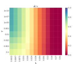
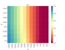
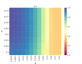
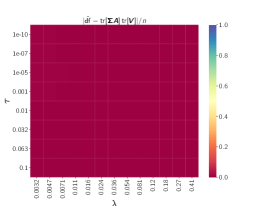
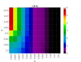
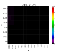
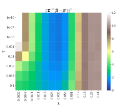
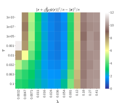
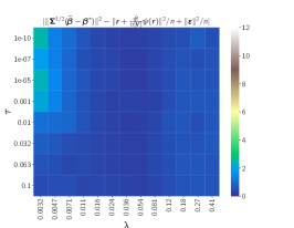
Figure 4: Heatmaps for the Huber loss and Elastic-Net penalty on a grid of tuning parameters with $\Lambda=0.054n^{1/2}$ and $(\lambda,\tau)$ where $\lambda\in[0.0032,0.41]$ and $\tau\in[10^{-10},0.1]$. Each cell is the average over 100 repetitions. See the simulation setup in Section 6 in the paper for more details.

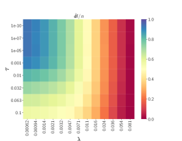
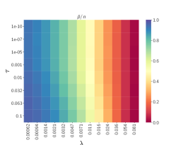
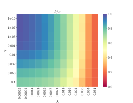
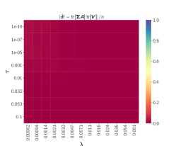
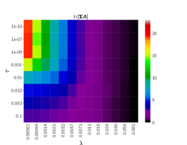
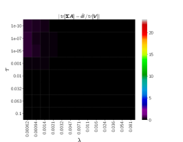
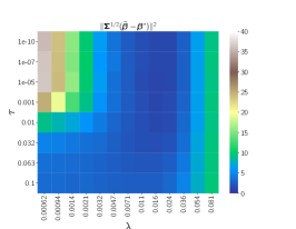
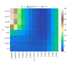
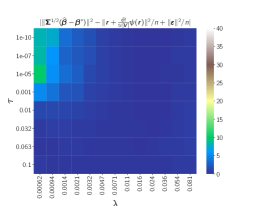
Figure 5: Heatmaps for the Huber loss and Elastic-Net penalty on a grid of tuning parameters with $\Lambda=0.024n^{1/2}$ and $(\lambda,\tau)$ where $\lambda\in[0.00062,0.081]$ and $\tau\in[10^{-10},0.1]$. Each cell is the average over 50 repetitions. See the simulation setup in Section 6 in the paper for more details.

11 Additional Figures (non-Gaussian, Rademacher design)

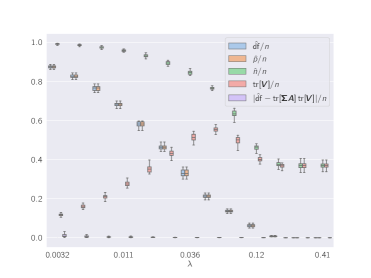
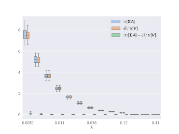
Figure 6: Boxplots for $\hat{\mathsf{df}},\hat{p},\hat{n},\operatorname*{tr}[\boldsymbol{V}],\operatorname*{tr}[\boldsymbol{\Sigma}{\widehat{\boldsymbol{A}}}]$ and $|\operatorname*{tr}[\boldsymbol{\Sigma}{\widehat{\boldsymbol{A}}}]-\hat{\mathsf{df}}/\operatorname*{tr}[\boldsymbol{V}]|$ in Huber Elastic-Net regression with $\tau=10^{-10}$ and $\lambda\in[0.0032,0.41].$ The data are generated with $\boldsymbol{X}$ having iid entries taking value $\pm 1$ each with probability 0.5 (so that $\boldsymbol{\Sigma}=\boldsymbol{I}_{p}$). Each box contains 30 data points.

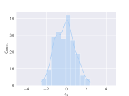
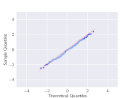
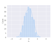
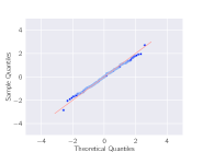
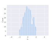
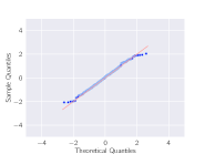
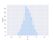
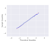
Figure 7: Histogram and QQ-plot for $\zeta_{1}$ in (13) under Huber Elastic-Net regression for different choices of tuning parameters $(\lambda,\tau)$. Left Top: $(0.036,10^{-10})$, Right Top: $(0.054,0.01)$, Left Bottom: $(0.036,0.01)$, Right Bottom: $(0.024,0.1)$. Each figure contains 100 data points generated with Rademacher design matrix (each entry has value $\pm 1$ with probability 0.5) and iid $\varepsilon_{i}$ from the $t$-distribution with 2 degrees of freedom.

References

• [1] Mohsen Bayati, Murat A Erdogdu, and Andrea Montanari. Estimating lasso risk and noise level. In Advances in Neural Information Processing Systems, pages 944–952, 2013.
• [2] Mohsen Bayati and Andrea Montanari. The lasso risk for gaussian matrices. IEEE Transactions on Information Theory, 58(4):1997–2017, 2012.
• [3] Pierre C Bellec. Out-of-sample error estimate for robust m-estimators with convex penalty. arXiv:2008.11840, 2020.
• [4] Pierre C Bellec and Cun-Hui Zhang. Second order stein: Sure for sure and other applications in high-dimensional inference. Annals of Statistics, accepted, to appear, 2018.
• [5] Pierre C Bellec and Cun-Hui Zhang. Second order poincare inequalities and de-biasing arbitrary convex regularizers when $p/n\to\gamma$. arXiv:1912.11943, 2019.
• [6] Stéphane Boucheron, Gábor Lugosi, and Pascal Massart. Concentration inequalities: A nonasymptotic theory of independence. Oxford University Press, 2013.
• [7] Michael Celentano and Andrea Montanari. Fundamental barriers to high-dimensional regression with convex penalties. arXiv preprint arXiv:1903.10603, 2019.
• [8] Michael Celentano, Andrea Montanari, and Yuting Wei. The lasso with general gaussian designs with applications to hypothesis testing. arXiv preprint arXiv:2007.13716, 2020.
• [9] Sourav Chatterjee. Fluctuations of eigenvalues and second order poincaré inequalities. Probability Theory and Related Fields, 143(1):1–40, 2009.
• [10] Kenneth R Davidson and Stanislaw J Szarek. Local operator theory, random matrices and banach spaces. Handbook of the geometry of Banach spaces, 1(317-366):131, 2001.
• [11] David Donoho and Andrea Montanari. High dimensional robust m-estimation: Asymptotic variance via approximate message passing. Probability Theory and Related Fields, 166(3-4):935–969, 2016.
• [12] Noureddine El Karoui, Derek Bean, Peter J Bickel, Chinghway Lim, and Bin Yu. On robust regression with high-dimensional predictors. Proceedings of the National Academy of Sciences, 110(36):14557–14562, 2013.
• [13] Iosif Pinelis (https://mathoverflow.net/users/36721/iosif pinelis). Large deviations: Growth of empirical average of iid non-negative random varialbes with infinite expectations? MathOverflow. URL:https://mathoverflow.net/q/390939 (version: 2021-05-24).
• [14] Vladimir A Marčenko and Leonid Andreevich Pastur. Distribution of eigenvalues for some sets of random matrices. Mathematics of the USSR-Sbornik, 1(4):457, 1967.
• [15] Léo Miolane and Andrea Montanari. The distribution of the lasso: Uniform control over sparse balls and adaptive parameter tuning. arXiv preprint arXiv:1811.01212, 2018.
• [16] Fabian Pedregosa, Gaël Varoquaux, Alexandre Gramfort, Vincent Michel, Bertrand Thirion, Olivier Grisel, Mathieu Blondel, Peter Prettenhofer, Ron Weiss, Vincent Dubourg, et al. Scikit-learn: Machine learning in python. the Journal of machine Learning research, 12:2825–2830, 2011.
• [17] Charles M Stein. Estimation of the mean of a multivariate normal distribution. The annals of Statistics, pages 1135–1151, 1981.
• [18] Mihailo Stojnic. A framework to characterize performance of lasso algorithms. arXiv preprint arXiv:1303.7291, 2013.
• [19] Christos Thrampoulidis, Ehsan Abbasi, and Babak Hassibi. Precise error analysis of regularized $m$-estimators in high dimensions. IEEE Transactions on Information Theory, 64(8):5592–5628, 2018.
• [20] William P Ziemer. Weakly differentiable functions: Sobolev spaces and functions of bounded variation, volume 120. Springer-Verlag New York, 1989.