Dual Training of Energy-Based Models
with Overparametrized Shallow Neural Networks

Abstract

Energy-based models (EBMs) are generative models that are usually trained via maximum likelihood estimation. This approach becomes challenging in generic situations where the trained energy is non-convex, due to the need to sample the Gibbs distribution associated with this energy. Using general Fenchel duality results, we derive variational principles dual to maximum likelihood EBMs with shallow overparametrized neural network energies, both in the feature-learning and lazy linearised regimes. In the feature-learning regime, this dual formulation justifies using a two time-scale gradient ascent-descent (GDA) training algorithm in which one updates concurrently the particles in the sample space and the neurons in the parameter space of the energy. We also consider a variant of this algorithm in which the particles are sometimes restarted at random samples drawn from the data set, and show that performing these restarts at every iteration step corresponds to score matching training. These results are illustrated in simple numerical experiments, which indicates that GDA performs best when features and particles are updated using similar time scales.

1 Introduction

Energy-based models (EBMs) are explicit generative models which consider Gibbs measures defined through an energy function $f$, with a probability density proportional to $\exp(-\beta f(x))$, where $\beta$ is the inverse temperature. Such models originate in statistical physics [Gibbs, 2010, Ruelle, 1969], and have become a fundamental modeling tool in statistics and machine learning [Wainwright and Jordan, 2008, Ranzato et al., 2007, LeCun et al., 2006, Du and Mordatch, 2019, Song and Kingma, 2021]. Given data samples from a target distribution, the learning algorithms for EBMs attempt to estimate an energy function $f$ to model the samples density. The resulting learned model can then be used to obtain new samples, typically through Markov Chain Monte Carlo (MCMC) techniques.

The standard method to train EBMs is maximum likelihood estimation, i.e. the learned energy is the one maximizing the likelihood of the target samples, within a certain function class. One generic approach for this is to use gradient descent, where gradients may be approximated using MCMC samples from the trained model. However, this is computationally difficult for highly non-convex trained energies, due to ‘metastability’, ie the presence of large basins in the energy landscape that trap trajectories for potentially exponential time. This has motivated a myriad of alternative losses to learn EBM energies, such as the popular score matching; see [Song and Kingma, 2021] for a review. All in all, such weaker losses result in a loss of statistical power, which motivates exploring computationally efficient methods for EBM maximum-likelihood estimation.

EBMs also have structural connections with maximum entropy (maxent) models, which have been studied for decades through Fenchel duality. Dai et al. [2019b] was the first work to leverage similar duality arguments for maximum likelihood EBM training. However, their analysis is restricted to energies lying in RKHS balls (i.e. non-parametric linear models). Despite the appealing optimization properties of RKHS, these spaces of functions typically only contain very smooth functions when the dimension is large [Berlinet and Thomas-Agnan, 2004]. A recent line of work—originating in supervised learning—has considered an alternative based on shallow neural networks [Bach, 2017], which admit a linear representation in terms of a measure over its parameters and are able to adapt to hidden low-dimensional structures in the data. The statistical benefits of the obtained $\mathcal{F}_{1}$ or Barron spaces have recently been studied in the context of shallow EBMs by Domingo-Enrich et al. [2021], who show that they may outperform the RKHS models.

2 Problem setup and main results

Consider a measurable set $\mathcal{X}\subseteq\mathbb{R}^{d_{1}}$ with a fixed base probability measure $\tau_{\mathcal{X}}\in\mathcal{P}(\mathcal{X})$. If $\mathcal{F}$ is a class of functions (or energies) mapping $\mathcal{X}$ to $\mathbb{R}$, for any $f\in\mathcal{F}$ we can define the probability measure $\nu_{\beta f}$ as a Gibbs measure with density:

$$\frac{d\nu_{\beta f}}{d\tau_{\mathcal{X}}}(x):=Z_{\beta f}^{-1}e^{-\beta f(x)}\text{ with }Z_{\beta f}:=\int_{\mathcal{X}}e^{-\beta f(y)}d\tau_{\mathcal{X}}(y)~{},$$ (1)

where $d\nu_{\beta f}/d\tau_{\mathcal{X}}$ is the Radon-Nikodym derivative of $\nu_{\beta f}$ and $Z_{\beta f}$ is the partition function and the parameter $\beta>0$ is the inverse temperature. Gibbs measures are the cornerstone of statistical physics since the seminal works of Boltzmann and Gibbs. Beyond their widespread use across computational sciences, they have also found their application in machine learning, by the name of energy-based models (EBMs), where the energy function is parametrized using a neural network.

Given samples $\{x_{i}\}_{i=1}^{n}$ from a target measure $\nu_{p}$, training an EBM consists in selecting the best $\nu_{\beta f}$ with energy $f\in\mathcal{F}$ according to a given criterion. The maximum likelihood estimator (MLE) is defined as the maximizer of the cross-entropy between $\nu_{\beta f}$ and the empirical measure $\nu_{n}=\frac{1}{n}\sum_{i=1}^{n}\delta_{x_{i}}$, $H(\nu_{\beta f},\nu_{n})=\int_{\mathcal{X}}\log(d\nu_{\beta f}/d\tau_{\mathcal{X}})d\nu_{n}$. Using the expression for $\nu_{\beta f}$ in (1), the MLE $\hat{f}$ is given by

$$\begin{split}\hat{f}=\operatorname*{argmax}_{f\in\mathcal{F}}\Big{\{}-\int_{\mathcal{X}}f(x)d\nu_{n}(x)-\beta^{-1}\log Z_{\beta f}\Big{\}}=\operatorname*{argmax}_{f\in\mathcal{F}}\Big{\{}-\frac{1}{n}\sum_{i=1}^{n}f(x_{i})-\beta^{-1}\log Z_{\beta f}\Big{\}}.\end{split}$$ (2)

The estimated distribution is then simply given by $d\nu_{\beta\hat{f}}=Z^{-1}_{\beta\hat{f}}e^{-\beta\hat{f}}d\tau_{\mathcal{X}}$. Since $D_{\text{KL}}(\nu||\nu^{\prime})=H(\nu,\nu)-H(\nu^{\prime},\nu)$, where $D_{\text{KL}}(\nu||\nu^{\prime})=\int_{\mathcal{X}}\log(d\nu/d\nu^{\prime})d\nu$ is the Kullback-Leibler (KL) divergence, observe that maximizing the cross-entropy would be equivalent to minimizing the KL divergence if the latter were finite.

Maximizing the objective in (2) is challenging because it contains the free energy functional $\log Z_{\beta f}$, which is unknown to us. One way to go around this difficulty is to realize that the gradient of $\log Z_{\beta f}$ over the parameters used to parametrize $\beta f$ can be expressed as an expectation over the the probability measure $\nu_{\beta f}$. For example, a simple calculation shows that

$$\partial_{\beta}\log Z_{\beta f}=-\int_{\mathcal{X}}f(x)d\nu_{\beta f}(x).$$ (3)

This offers the possibility to maximize the objective in (2) by stochastic gradient ascent (SGA) by estimating the gradient of (2) at every SGA step via sampling of $\nu_{\beta f}$, which can be done, for example, via Metropolis-Hastings Monte-Carlo. From a functional standpoint, this amounts to replacing the maximization problem in (2) by the max-min

$$\max_{f\in\mathcal{F}}\min_{\nu\in\mathcal{P}(\mathcal{X})}\int_{\mathcal{X}}f(d\nu-d\nu_{n})+\beta^{-1}D_{\text{KL}}(\nu||\tau_{\mathcal{X}})$$ (4)

Indeed the minimization over $\nu\in\mathcal{P}(\mathcal{X})$ can be carried explicitly and brings us back to (2).

Reformulating the problem as the max-min in (4) also indicates why proceeding this way may not be optimal from computational standpoint. Indeed, sampling $\nu_{\beta f}$ to estimate the gradient of the objective (2) at every step of training by SGA is typically tedious and costly, and it would be better to amortize this computation along the training. This suggests to perform the minimization and the maximization in (4) concurrently rather than in sequence. In practice this can be done using stochastic gradient descent-ascent (SGDA) to simultaneously train the energy $f$ and sample its associated Gibbs measure $\nu_{\beta f}$, using timescales for both that can be adjusted for efficiency. A necessary condition for the convergence of concurrent SGDA is that the min and the max in (4) commute, i.e. the optimal value and optimal solutions of (4) are equal to the ones of the problem

$$\min_{\nu\in\mathcal{P}(\mathcal{X})}\max_{f\in\mathcal{F}}\int_{\mathcal{X}}f(d\nu-d\nu_{n})+\beta^{-1}D_{\text{KL}}(\nu||\tau_{\mathcal{X}}).$$ (5)

A main theoretical contribution of the present paper is to use infinite-dimensional Fenchel duality results to show the equivalence between (4) and (5) for energies $f$ that belong to metric ball of Barron space $\mathcal{F}_{1}$, which is a Banach space containing infinitely-wide neural networks. While the duality between (4) and (5) is only a necessary condition for the convergence of SGDA, we observe that it does work in practice by performing experiments with shallow neural network energies and investigating which relative timescales in SGDA lead to faster convergence.

We also show that a simple modification of this SGDA algorithm interpolates between standard MLE training on (4) and training using score matching (SM), which is another objective function used to train EBMs that has gained popularity in recent years. The SM metric or relative Fisher information between two absolutely continuous probability measures $\nu,\nu^{\prime}$ is defined as $\text{SM}(\nu,\nu^{\prime})=\int_{\mathcal{X}}|\nabla\log\frac{d\nu}{d\tau_{\mathcal{X}}}(x)-\nabla\log\frac{d\nu^{\prime}}{d\tau_{\mathcal{X}}}(x)|^{2}\ d\nu(x)$. The key insight from Hyvärinen [2005] is that via integration by parts this quantity may be rewritten without involving the log-density of $\nu$, which leads to the following loss function:

$$\begin{split}\min_{f\in\mathcal{F}}\frac{1}{n}\sum_{i=1}^{n}\beta^{-1}\Delta f(x_{i})+\frac{1}{2}|\nabla f(x_{i})|^{2}=\min_{f\in\mathcal{F}}\int_{\mathcal{X}}\left(\beta^{-1}\Delta f(x)+\frac{1}{2}|\nabla f(x)|^{2}\right)d\nu_{n}(x)\end{split}$$ (6)

Score matching is computationally more tractable than maximum likelihood because it avoids estimating the partition function $Z_{\beta f}$ or its gradient altogether. However, it has the known drawback that it may fail to distinguish distributions in some instances—this is because the SM metric is weaker than the KL divergence.

Related work. Our work is based on general Fenchel duality results (App. B) that may be useful in applications beyond the main focus of this paper (see App. D). These theorems are a generalization of results stated in the compact case in Domingo-Enrich et al. [2021] in their Appendix D. Similar duality results have been studied extensively in the area of maximum entropy (maxent) models (reviewed in Ch. 12 of Mohri et al. [2012]). The first maxent duality principle was due to Jaynes [1957]. Maxent models have been applied since the 1990s in natural language processing and in species habitat modeling among others, and studied theoretically especially since the 2000s [Altun and Smola, 2006, Dudík et al., 2007].

Recently Dai et al. [2019a] leveraged duality arguments in the context of maximum likelihood EBMs, although in a form different from ours. Their duality result works in the more restrictive setting of “lazy” energies lying in RKHS balls and probability measures with $L^{2}$ densities, and they derive it directly from a general theorem that works for reflexive Banach spaces [Ekeland and Temam, 1999, Ch. 6, Thm. 2.1]. Our Fenchel duality results, which work for Borel probability measures and feature-learning ($\mathcal{F}_{1}$) energies, are more general because we must rely on measure spaces, which are non-reflexive Banach spaces. Their algorithm is also different: they do not evolve generated samples, but rather use a transport parametrization of the energy. Dai et al. [2019b] expand the work [Dai et al., 2019a] combining it with Hamiltonian Monte Carlo.

A precursor of modern machine learning EBMs were restricted Boltzmann machines (RBMs), first trained via contrastive divergence or CD [Hinton, 2002] - which estimates the gradient of the log-likelihood via approximate MCMC samples of the trained model. It later led to maximum likelihood training of EBMs [see, e.g., Xie et al., 2016, 2017, Du and Mordatch, 2019, among others]. A popular variant of CD is persistent contrastive divergence or PCD [Tieleman, 2008, Tieleman and Hinton, 2009], in which the MCMC samples are evolved and reused over gradient computations to be progressively equilibrated. Training EBMs by updating the energy parameters and the samples simulteanously like we do resembles PCD.

A vast array of EBM losses alternative to maximum likelihood have been developed recently [Song and Kingma, 2021] with the goal of avoiding the MCMC procedure, e.g. score matching [Hyvärinen, 2005] and related methods such as denoising score matching [Vincent, 2011], and score-based generative modeling [Song and Ermon, 2019, 2020, Ho et al., 2020, Song et al., 2021]. Our work should also be contrasted with the literature on convergence for minimax problems: Heusel et al. [2017], Lin et al. [2020] among others argue for two-timescale GDA and SGDA, while our experiments show the benefits of simultaneous training, suggesting that further work is needed for clarification.

Finally, App. C has links with maximum mean discrepancy (MMD) flows. MMDs are probability metrics that were first introduced by Gretton et al. [2007, 2012] for kernel two-sample tests, and that have been successful as discriminating metrics in generative modeling [Li et al., 2015, Dziugaite et al., 2015, Li et al., 2017]. Arbel et al. [2019] study theoretically the convergence of unregularized MMD gradient flow (our equation (36) with $\tilde{\beta}^{-1}=0$). In their experiments, they observe that noisy updates ($\tilde{\beta}^{-1}>0$) are needed for good generalization. Our work shows that their algorithm is exactly training maximum likelihood EBMs energies in an RKHS ball of radius that depends on the noise level.

3 Background

In this section, we provide preliminary background on the Barron space $\mathcal{F}_{1}$, and on the specific form of EBM losses for this type of energies.

Notation. If $V$ is a normed vector space, $\mathcal{B}_{V}(\beta)$ denotes the closed ball of $V$ of radius $\beta$, and $\mathcal{B}_{V}:=\mathcal{B}_{V}(1)$. If $K$ is a subset of the Euclidean space, $\mathcal{P}(K)$ is the set of Borel probability measures, $\mathcal{M}(K)$ is the space of Radon (i.e. signed and finite) measures, and $\mathcal{M}^{+}(K)$ is the set of non-negative Radon measures. If $\gamma\in\mathcal{M}(K)$, then ${\|\gamma\|}_{\text{TV}}=\int_{K}d|\gamma|$ is the total variation (TV) norm of $\gamma$, which turns $\mathcal{M}(K)$ into a Banach space. Unless otherwise specified, $\sigma:\mathbb{R}\to\mathbb{R}$ is a generic non-linear activation function. The ReLU activation is denoted by $(z)_{+}=\max\{z,0\}$. $\tau$ denotes a fixed base probability measure; a subindex specifies the space it is defined over. $\mathbb{S}^{d}\subseteq\mathbb{R}^{d+1}$ is the $d$-dimensional hypersphere; $\log$ is the natural logarithm; $\lambda$ is the Lebesgue measure. Given $\nu,\nu^{\prime}\in\mathcal{P}(K)$, $D_{\text{KL}}(\nu\|\nu^{\prime})=\int_{K}\log\frac{d\nu}{d\nu^{\prime}}\ d\nu$ is the KL divergence and $H(\nu,\nu^{\prime})=-\int_{K}\log(\frac{d\nu^{\prime}}{d\tau})d\nu$ is the cross-entropy.

The Barron space $\mathcal{F}_{1}$. Let $\mathcal{X}\subseteq\mathbb{R}^{d_{1}}$, $\Theta\subseteq\mathbb{R}^{d_{2}}$, $\varphi:\mathcal{X}\times\Theta\to\mathbb{R}$, and $\tau_{\Theta}$ be a fixed base probability measure over $\Theta$. $\mathcal{F}_{1}$ is defined as the Banach space of functions $f:\mathcal{X}\rightarrow\mathbb{R}$ such that, for some Radon measure $\gamma\in\mathcal{M}(\Theta)$, for all $x\in\mathcal{X}$ we have $f(x)=\int_{\Theta}\varphi(x,\theta)\ d\gamma(\theta)$. We define the norm of $\mathcal{F}_{1}$ as $\|f\|_{\mathcal{F}_{1}}=\inf\left\{{\|\gamma\|}_{\text{TV}}\ |f(\cdot)=\int_{\Theta}\varphi(\cdot,\theta)\ d\gamma(\theta)\right\}.$ This construction was introduced by Bach [2017], who first used the notation $\mathcal{F}_{1}$ and focused in particular on the case $\mathcal{X}\subseteq\mathbb{R}^{d}$, $\Theta=\mathbb{S}^{d}$ and $\varphi(x,\theta)=\text{ReLu}^{k}(\langle(x,1),\theta\rangle)$ for some $k\in\mathbb{Z}_{+}$. This space is also known by the name of Barron space [E et al., 2019, E and Wojtowytsch, 2020] in reference to the classic work Barron [1993].

We denote by $\mathcal{F}_{1}$-EBMs the energy-based models for which the energy class $\mathcal{F}$ is the unit ball $\mathcal{B}_{\mathcal{F}_{1}}(1)$ of $\mathcal{F}_{1}$. Notice that the class $\{\beta f|f\in\mathcal{F}\}$ is equal to the ball $\mathcal{B}_{\mathcal{F}_{1}}(\beta)$. Such models may be regarded as abstractions of more complex deep EBMs, in that they incorporate feature learning, and they were first studied by Domingo-Enrich et al. [2021], which provide statistical guarantees. They are to be contrasted with $\mathcal{F}_{2}$-EBMs, for which $\mathcal{F}$ is the unit ball $\mathcal{B}_{\mathcal{F}_{2}}(1)$. $\mathcal{F}_{2}$-EBMs, which we study in App. C, have fixed features and showed worse statistical performance in experiments [Domingo-Enrich et al., 2021].

Maximum likelihood for $\mathcal{F}_{1}$-EBMs. We rewrite the maximum likelihood problem (2) for the case in which $\mathcal{F}=\mathcal{B}_{\mathcal{F}_{1}}(1)$. Since an arbitrary element $f$ of $\mathcal{F}_{1}$ can be expressed as $f(x)=\int_{\Theta}\varphi(x,\theta)\ d\gamma(\theta)$, with $\|f\|_{\mathcal{F}_{1}}$ equal to the infimum of $\|\gamma\|_{\text{TV}}$ for all such $\gamma$, the maximum likelihood energy is $f_{\text{MLE}}=\int_{\Omega}\varphi(\cdot,\theta)d\gamma_{\text{MLE}}(\theta)$, where

$$\begin{split}\gamma_{\text{MLE}}=\operatorname*{argmin}_{\begin{subarray}{c}\gamma\in\mathcal{M}(\Theta)\\ \|\gamma\|_{\text{TV}}\leq 1\end{subarray}}\bigg{\{}\frac{1}{n}\sum_{i=1}^{n}\int_{\Theta}\varphi(x_{i},\theta)\ d\gamma(\theta)+\frac{1}{\beta}\log\bigg{(}\int_{\mathcal{X}}\exp\left(-\beta\int_{\Theta}\varphi(x,\theta)\ d\gamma(\theta)\right)d\tau_{\mathcal{X}}(x)\bigg{)}\bigg{\}}.\end{split}$$ (7)

Score matching for $\mathcal{F}_{1}$-EBMs. Suppose that $\mathcal{X}\subseteq\mathbb{R}^{d_{1}}$ is a manifold without boundaries. Assume that $\int_{\mathcal{X}}|\nabla_{x}\varphi(x,\theta)\cdot\nabla\frac{d\nu_{p}}{d\tau_{\mathcal{X}}}(x)|\ d\tau_{\mathcal{X}}(x)$ is upper-bounded by some constant $K$ for all $\theta\in\Theta$. Assume also that $\sup_{\theta\in\Theta}\|\nabla_{x}\varphi(x,\theta)\|<\eta(x)$ and that $\int_{\mathcal{X}}|\eta(x)|^{2}\ d\nu_{p}(x)<\infty$. 6 in App. G shows that the optimal energy under the score matching loss with energy class $\mathcal{B}_{\mathcal{F}_{1}}(1)$ is $f_{\rm SM}=\int_{\Omega}\varphi(\cdot,\theta)d\gamma_{\rm SM}(\theta)$ where

$$\begin{split}\gamma_{\rm SM}=\operatorname*{argmin}_{\begin{subarray}{c}\gamma\in\mathcal{M}(\Theta)\\ \|\gamma\|_{\text{TV}}\leq 1\end{subarray}}\int_{\Theta}\int_{\mathcal{X}}\bigg{(}\frac{\nabla_{x}\varphi(x,\theta)}{2}\cdot\nabla_{x}\int_{\Theta}\varphi(x,\theta^{\prime})\ d\gamma(\theta^{\prime})-\beta^{-1}\Delta_{x}\varphi(x,\theta)\bigg{)}d\nu_{n}(x)d\gamma(\theta).\end{split}$$ (8)

4 Duality for $\mathcal{F}_{1}$-EBMs

As a corollary of the duality result from Subsec. B.2, we derive an alternative objective for $\mathcal{F}_{1}$-EBMs trained via maximum likelihood, the original objective being (7) and we develop an algorithm to solve this alternative problem. To this end, we make:

Assumption 1.

Let $\varphi:\mathcal{X}\times\Theta\to\mathbb{R}$ be a continuous function such that either $\mathcal{X}$ is compact or (i) for any fixed $\theta\in\Theta$, $\varphi(x,\theta)\leq\xi(x)$ for some strictly positive $\xi:\mathcal{X}\to\mathbb{R}$, and (ii) $\xi(x)+\log(\xi(x))=o\left(-\log\left(\frac{d\tau_{\mathcal{X}}}{d\lambda}(x)\right)-(d_{1}+\epsilon)\log\|x\|_{2}\right)\text{ as }\|x\|_{2}\to\infty$ for some $\epsilon>0$.

In particular, this assumption holds for ReLU network energies when setting $\mathcal{X}=\mathbb{R}^{d_{1}}$, $\Theta=\mathbb{R}^{d_{1}+1}$, $\varphi(x,\theta)=\sigma(\langle(x,1),\theta\rangle)/\|\theta\|$ and $\tau_{\mathcal{X}}$ Gaussian (and in many other settings).

Theorem 1.

Under Assumption 1, the maximum likelihood problem (7) is the Fenchel dual of

$$\begin{split}\min_{\nu\in\mathcal{P}(\mathcal{X})}\max_{\begin{subarray}{c}\gamma\in\mathcal{M}(\Theta),\\ \|\gamma\|_{\text{TV}}\leq 1\end{subarray}}\bigg{\{}\beta^{-1}D_{\text{KL}}(\nu||\tau_{\mathcal{X}})+\int_{\Theta}\int_{\mathcal{X}}\varphi(x,\theta)\ d(\nu-\nu_{n})(x)\ d\gamma(\theta)\bigg{\}}.\end{split}$$ (9)

Moreover, the solution $\nu^{\star}$ of (123) is precisely the Gibbs measure for the optimal $\gamma^{\star}$ in (7), that is, $\frac{d\nu^{\star}}{d\tau_{\mathcal{X}}}(x)=\frac{1}{Z_{\beta}}\exp\left(-\beta\int_{\Theta}\varphi(x,\theta)\ d\gamma^{\star}(x)\right)$.

As mentioned in Sec. 2, Theorem 1 shows that the min with respect to the probability measure $\nu$ and the max with respect to the parameter measure $\mu$ can be exchanged; the optimal values and the minimax points of both problems coincide. This puts in more solid footing the tuning of timescales that we propose in the next section and analyze experimentally in Sec. 7. In Theorem 1, if we replace the $\mathcal{F}_{1}$ ball by the unit ball of the related space $\mathcal{F}_{2}$, an analogous duality result links the maximum likelihood problem with the entropy regularized MMD flow from Arbel et al. [2019] (see App. C).

5 Algorithm for $\mathcal{F}_{1}$-EBMs

In this section we introduce measure dynamics to solve the minimax problems (7)-(9). We consider the triple $(\gamma^{+},\gamma^{-},\nu)$ where the nonegative measures $\gamma^{\pm}$ are defined through the Hahn decomposition of $\gamma=\gamma_{+}-\gamma_{-}$. Then we introduce coupled gradient flows for this triple, in which $\gamma^{+}_{t}$ and $\gamma^{-}_{t}$ evolve via a Wasserstein-Fisher-Rao gradient flow [Chizat et al., 2018] and $\nu_{t}$ evolves via a Wasserstein gradient flow [Santambrogio, 2017]:

$$\begin{split}\partial_{t}\gamma^{\sigma}_{t}&=-\alpha\sigma\nabla_{\theta}\cdot\left(\gamma^{\sigma}_{t}\nabla_{\theta}F_{t}(\theta)\right)+\alpha\gamma^{\sigma}_{t}\left(\sigma F_{t}(\theta)-K_{t}\right),\quad\text{where}\ \ \sigma=\pm 1,\ \ \gamma_{t}^{\sigma}=\gamma_{t}^{\pm}\\ \partial_{t}\nu_{t}&=\nabla_{x}\cdot\bigg{(}\nu_{t}\left(\nabla_{x}f_{t}(x)-\beta^{-1}\nabla\log\frac{d\tau_{\mathcal{X}}}{d\lambda}\right)\bigg{)}+\beta^{-1}\Delta_{x}\nu_{t},\end{split}$$ (10)

where $\alpha$ is a tunable parameter and we defined

$$\begin{split}F_{t}(\theta)&=\int_{\mathcal{X}}\varphi(x,\theta)\ d(\nu_{t}\!-\!\nu_{n})(x),\quad f_{t}(x)=\int_{\Theta}{\varphi}(x,\theta)\ (d\gamma_{t}^{+}-d\gamma^{-}_{t})(\theta),\\ K_{t}&=\mathds{1}_{\|\gamma^{+}_{t}\|_{\text{TV}}+\|\gamma^{-}_{t}\|_{\text{TV}}\geq 1}\int_{\Theta}F_{t}(\theta)(d\gamma_{t}^{+}-d\gamma^{-}_{t})(\theta).\end{split}$$ (11)

The initialization of (10) is $\nu_{0}=\nu_{n}$ and $\gamma_{0}^{\pm}=0$ (such that the initial energy is null). The term $K_{t}$ keeps the total variation of $\gamma_{t}$ below one. The parameter $\alpha$ acts as a relative timescale. Notice that different values of $\alpha$ lead to different behaviors of the dynamics. Setting $\alpha\ll 1$ corresponds heuristically to solving the primal formulation of maximum likelihood with persistent MCMC samples (equation (7)), as the measures $\gamma^{\pm}_{t}$ on neurons evolve slower than the measure $\nu_{t}$ on particles. In contrast if $\alpha\gg 1$, $\gamma^{\pm}_{t}$ evolves faster than $\nu_{t}$ and if the optimization is well behaved, at all times $\gamma_{t}=\gamma^{+}_{t}-\gamma^{-}_{t}$ remains close to minimizing the inner maximization problem of (9) with $\gamma=\gamma_{t}$. Thus, $\alpha\gg 1$ is heuristically solving (9). The experiments in the next section suggest that $\alpha\approx 1$ yields the fastest convergence computationally.

1 below states that the solution $(\mu_{t},\nu_{t})$ may be approximated using coupled particle systems (see proof in App. F) and is the basis for Alg. 1. The link between particle systems and measure PDEs is through a classical technique known as propagation of chaos [Sznitman, 1991] and it has been used previously for similar coupled systems in the machine learning literature [Domingo-Enrich et al., 2020], as well as to analyze the convergence of gradient descent for infinite-width neural networks [Rotskoff and Vanden-Eijnden, 2018, Mei et al., 2018, Chizat and Bach, 2018].

Proposition 1.

Let $\{\theta_{0}^{(j)}\}_{j=1}^{m}$ be initial features sampled uniformly over $\Theta$, let $\{\sigma_{j}\}_{j=1}^{m}$ be uniform samples over $\{\pm 1\}$ and let $\{w_{0}^{(j)}=1\}_{j=1}^{m}$ be the initial weight values, which are set to 1. Let $\{X_{0}^{(i)}\}_{i=1}^{N}$ be the initial “generated” samples, which are chosen i.i.d. uniformly from the target sample set $\{x_{i}\}_{i=1}^{n}$. Consider the system of ODEs/SDEs:

$$\begin{split}\frac{d\theta_{t}^{(j)}}{dt}&=\alpha\sigma_{j}\nabla\tilde{F}_{t}(\theta_{t}^{(j)}),\quad\frac{dw_{t}^{(j)}}{dt}=\alpha w_{t}^{(j)}(\sigma_{j}\tilde{F}_{t}(\theta_{t}^{(j)})-\tilde{K}_{t})\\ dX_{t}^{(i)}&=\left(-\nabla\tilde{f}_{t}(X_{t}^{(i)})+\beta^{-1}\nabla\log\frac{d\tau_{\mathcal{X}}}{d\lambda}(X_{t}^{(i)})\right)\ dt+\sqrt{2\beta^{-1}}\ dW_{t}^{(i)}\end{split}$$ (12)

where

$$\begin{split}\tilde{F}_{t}(\theta)&=\frac{1}{N}\sum_{i=1}^{N}\varphi(X_{t}^{(i)},\theta)-\frac{1}{n}\sum_{i=1}^{n}\varphi(x_{i},\theta),\quad\tilde{f}_{t}(x)=\frac{1}{m}\sum_{j=1}^{m}\sigma_{j}w^{(j)}_{t}\varphi(x,\theta^{(j)}_{t}),\\ \tilde{K_{t}}&=\mathds{1}_{\sum_{j=1}^{m}w^{(j)}_{t}\geq m}\ \frac{1}{m}\sum_{j=1}^{m}\sigma_{j}w^{(j)}_{t}\tilde{F}_{t}(\theta_{t}^{(j)}).\end{split}$$ (13)

are the empirical counterparts of the functions in (11). Then the system (12) approximates the measure dynamics. Namely, as $m,N\rightarrow\infty$:

• the empirical measure $\hat{\gamma}_{t}=\frac{1}{m}\sum_{j=1}^{m}\sigma_{j}w_{t}^{(j)}\delta_{\theta_{t}^{(j)}}$ converges weakly to the solution $\gamma_{t}=\gamma_{t}^{+}-\gamma_{t}^{-}$ of (10) with uniform initialization for any finite time interval $[0,T]$, and

• the empirical measure $\hat{\nu}_{t}=\frac{1}{N}\sum_{i=1}^{N}\delta_{X_{t}^{(i)}}$ converges weakly to the solution $\nu_{t}$ of (10) for any finite time interval $[0,T]$.

Importantly, the system of ODEs/SDEs in (12) may be solved via forward Euler steps on $\{\theta_{j}\}_{j=1}^{m}$ and $\{w_{j}\}_{j=1}^{m}$ (or rather, $\{\log w_{j}\}_{j=1}^{m}$), and Euler-Maruyama updates on $\{X_{0}^{(i)}\}_{i=1}^{N}$. Such a discretization yields Alg. 1. We reemphasize that when $\alpha\ll 1$, Alg. 1 is simply the classical maximum likehilood algorithm with persistent particles (up to the minor detail that gradient descent is applied to $\log w^{(j)}$ instead of $w^{(j)}$).

Algorithm 1 Dual $\mathcal{F}_{1}$-EBM training

  Input: $n$ samples $\{x_{i}\}_{i=1}^{n}$ of the target distribution, stepsize $s$, stepsize ratio $\alpha$.

  Initialize features $(\theta_{0}^{(j)})_{j=1}^{m}$ uniformly over $\Theta$, weights $(w_{0}^{(j)})_{j=1}^{m}$ in $[0,1)$, signs $(\sigma_{j})_{j=1}^{m}$ over $\{\pm 1\}$. Initialize generated samples $\{X_{0}^{(i)}\}_{i=1}^{N}$ unif. i.i.d. from $\{x_{i}\}_{i=1}^{n}$.

  for $t=0,\dots,T-1$ do

     for $i=1,\dots,N$ do

        Sample $\zeta_{t}^{(i)}$ from the $d_{1}$-variate standard Gaussian.

        Perform Euler-Maruyama update: $X_{t+1}^{(i)}=X_{t}^{(i)}-s(\nabla\tilde{f}_{t}(X_{t}^{(i)})+\beta^{-1}\nabla\log\frac{d\tau_{\mathcal{X}}}{d\lambda}(X_{t}^{(i)}))+\sqrt{2\beta^{-1}s}\,\zeta_{t}^{(i)}$, where $\tilde{f}_{t}$ is defined in (13).

     end for

     for $j=1,\dots,m$ do

        Update $\theta_{t+1}^{(j)}=\theta_{t}^{(j)}+s\alpha\sigma_{j}\nabla\tilde{F}_{t}(\theta_{t}^{(j)})$, where $\tilde{F}_{t}$ is defined in (13).

        Update $\tilde{w}_{t+1}^{(j)}=w_{t+1}^{(j)}\exp(s\alpha\sigma_{j}\tilde{F}_{t}(\theta_{t}^{(j)}))$.

        Normalize, when it is needed: $w_{t+1}^{(j)}=\tilde{w}_{t+1}^{(j)}/\max\left(\frac{1}{m}\sum_{j^{\prime}=1}^{m}\tilde{w}_{t+1}^{(j^{\prime})},1\right)$.

     end for

  end for

  Output: samples $\{X_{T}^{(i)}\}_{i=1}^{N}$, energy $f_{T}(x):=\frac{\beta}{m}\sum_{j=1}^{m}\sigma_{j}w_{j}\varphi(x,\theta_{j})$.

6 Links between maximum likelihood and score matching $\mathcal{F}_{1}$-EBMs

In this section we uncover how the score matching loss fits seamlessly as a variant of Alg. 1, in the form of particle restarts. Interestingly, we can modify the PDE (10) in a way that allows us to make a connection with score matching. To this end, let us introduce the following coupled measure PDE:

$$\begin{split}\partial_{t}\gamma^{\sigma}_{t}&=-\alpha\sigma\nabla_{\theta}\cdot\left(\gamma^{\sigma}_{t}\nabla_{\theta}F_{t}(\theta)\right)+\alpha\gamma^{\sigma}_{t}\left(\sigma F_{t}(\theta)-K_{t}\right),\\ \partial_{t}\nu_{t}&=\nabla_{x}\cdot\left(\nu_{t}\left(\nabla_{x}f_{t}(x)-\beta^{-1}\nabla\log\frac{d\tau_{\mathcal{X}}}{d\lambda}\right)\right)+\beta^{-1}\Delta_{x}\nu_{t}-\alpha\left(\nu_{t}-\nu_{n}\right).\end{split}$$ (14)

Remark that the only difference between this equation and the PDE (10) for dual maximum likelihood training is the term $-\alpha(\nu_{t}-\nu_{n})$, which draws $\nu_{t}$ closer to the empirical target measure $\nu_{n}$. We have:

Proposition 2.

In the limit $\alpha\to\infty$, the equations for $\gamma^{\sigma}_{t}$ in (14) reduce to

$$\partial_{t}\gamma^{\sigma}_{t}=\sigma\nabla_{\theta}\cdot\left(\gamma^{\sigma}_{t}\nabla_{\theta}V(\gamma_{t})(\theta)\right)-\gamma^{\sigma}_{t}\left(\sigma V(\gamma_{t})(\theta)-\bar{V}(\gamma_{t})\right),$$ (15)

where $\gamma_{t}=\gamma^{+}_{t}-\gamma^{-}_{t}$, $\bar{V}(\gamma)=\int_{\Theta}V(\gamma)\,d\gamma$, and $V(\gamma)(\theta)$ is the Frechet derivative of the score matching loss $L:\mathcal{M}(\Theta)\rightarrow\mathbb{R}$ defined in (8).

That is, in the large $\alpha$ limit, equation (14) is equivalent to the Wasserstein-Fisher-Rao gradient flow of a loss $L$ which, remarkably, is the score matching loss for $\mathcal{F}_{1}$-EBMs. This means that adding the term $-\alpha\left(\nu_{t}-\nu_{n}\right)$ to the dual maximum likelihood measure dynamics and letting $\alpha\to\infty$ we recover the score matching dynamics. This additional term can be easily implemented at particle level by replacing each training sample $X_{t}^{(i)}$ by some random target sample in $\{x_{i}\}_{i=1}^{n}$ with probability $p_{R}=1-e^{-\alpha t}=\alpha t+o(t)$ for every time interval of length $t$ (proof in App. G). Similar birth-death processes were used in [Rotskoff et al., 2019] in the context of neural network regression. Hence, the score matching scheme corresponds to modifying Alg. 1 by restarting each sample $X^{(i)}_{t}$ as a uniformly chosen sample in $\{x_{i}\}_{i=1}^{n}$ with probability $p_{R}=s\alpha$, right before the Euler Maruyama update. The restart probability acts as a knob that allows us to interpolate between score matching and maximum likelihood. In the experimental simulations we use a parameter $\alpha^{\prime}$ different from $\alpha$ for the reinjection term, to study a wider range of behaviors.

In summary, score matching differs from dual maximum likelihood in that the trained measure is being “pulled” towards the target measure at all times via particle restarting. Such constant pulling should be useful to alleviate sampling problems due to metastability issues which may arise with dual maximum likelihood. However, dual maximum likelihood has the upside of providing samples of the learned EBM as a byproduct of training, which score matching does not. It is also interesting to contrast our approach to score matching with the works Sutherland et al. [2018], Arbel and Gretton [2018], which using different techniques propose algorithms to train EBMs with RKHS energies via score matching; the connection that we identify between maximum likelihood and score matching is novel. Finally, notice that a particle discretization of the flow (15) yields an alternative straightforward algorithm to train $\mathcal{F}_{1}$-EBMs via score matching (see Subsec. G.1), which can be linked directly to Alg. 1 with particle restarts.

7 Experiments

We perform two sets of experiments. Our first set of experiments involves simulating the measure PDEs in dimension 1 to understand which timescale $\alpha$ provides better convergence properties, and whether particle restarts help. Since the dimension is low, we solve the PDEs exactly by gridding the space and do not need to resort to particle dynamics. In our second set of experiments we apply Alg. 1 to high-dimensional spheres.

7.1 PDE simulations

Setup. In the notation of Sec. 3, we set both the base space $\mathcal{X}$ and the parameter space $\Theta$ to be the 1-dimensional torus $[0,1]$ (i.e. with periodic boundary conditions). We set $\varphi:\mathcal{X}\times\Theta\to\mathbb{R}$ as a Gaussian with fixed variance $\delta^{2}$: $\varphi(x,\theta)=\sum_{k\in\mathbb{Z}}\exp(2i\pi k(x-\theta)-\frac{1}{2}\delta^{2}k^{2})$. We define the target measure $\nu_{p}$ with energy $E_{p}(x)=\int_{\Theta}\varphi(x,\theta)g(\theta)\,d\theta$, where $g(\theta)=-\log(p\exp(a_{1}\cos(2\pi(\theta-\bar{\theta}_{1}))-a_{1})+q\exp(a_{2}\cos(2\pi(\theta-\bar{\theta}_{2})-a_{2}))$ with $q=1-p$. The measure $\nu_{p}$ and the energy $E_{p}$ are shown in Figure 1. $\nu_{p}$ is bimodal: $p,q=1-p>0$ control the relative size of the modes and $a_{1}>0$, $a_{2}>0$ control their width. Note that $E_{p}$ belongs to the space $\mathcal{F}_{1}$, which means that the target energy may be recovered exactly. We work with the population loss so that there is no statistical error. Consistently, we use no regularization term in the equation for $\gamma_{t}^{\sigma}$ in 14 ($K_{t}=0$), and we only consider $\sigma=-1$ since the target $g_{p}$ is negative. For simplicity we also neglect the transport term in the equation for $\gamma_{t}^{\sigma}$ in 14 and we set $\tau_{\mathcal{X}}=\lambda$ in the equation for $\nu_{t}$. These PDE are solved using a pseudo-spectral code with an exponential integrator in time.

Figure 1: (Left) Energy $E_{p}$ of the target distribution in blue, learned energy in red and minus log-density of $\nu_{t}$ in yellow. (Center) Target density in blue, density computed from learned energy in red, $\nu_{t}$ in yellow. (Right) Evolution of the KL computed with respect to the learned EBM in blue, of the KL with respect to $\nu_{t}$ in yellow, and of the SM metric in red.

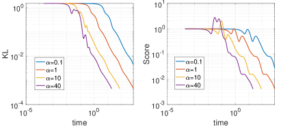
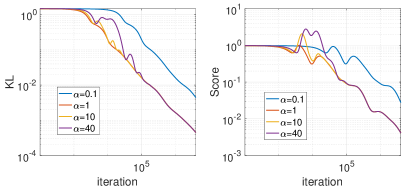
Figure 2: (Left figures) Evolution of the KL divergence and SM metric between the target and learned distributions in the physical (real) time, for different values of $\alpha$. (Right figures) Same curves with time rescaled by $\max\{\alpha,1\}$.

Figure 3: Evolution of the KL and the SM for the measure PDE with different intensities of particle reinjection. For all the curves, $\alpha=10$ and $\alpha^{\prime}$ is the parameter in the reinjection term $-\alpha^{\prime}(\nu_{t}-\nu_{n})$. Times are rescaled by $\max\{\alpha,1\}$.

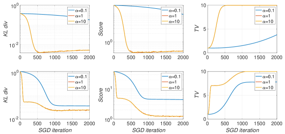
Figure 4: (Top) The evolution of the KL divergence, the score matching metric and the TV norm of the trained measure (i.e., the $\mathcal{F}_{1}$ norm) during training for Algorithm 1 with $\mathcal{X}=\mathbb{S}^{14}$, $m=64$, $p_{R}=0$, $s=0.02$, $n=10^{5}$, $N=2\cdot 10^{5}$ and $\alpha=0.1,1,10$, showing a speedup by a factor about 10-20 of the latter over the former. The angle between the two teacher neurons is 1.37 rad (monomodal distribution). (Bottom) Same experiments with an angle of 2.87 rad (bimodal distribution).

Results. Figure 2 and Figure 3 show the evolution of the KL divergence and SM metric between the target measure $\nu_{p}$ and learned measure over training. Two time parametrizations are shown: the small plots are in the time of the PDEs (10)-(14), while in the large plots the time of each curve is rescaled by multiplying it by $\max\{\alpha,1\}$. The reason behind the rescaling is that computationally the timestep needs to be proportional to $\min\{\alpha,1\}$ to avoid numerical instabilities at the faster timescale. Thus, for algorithmic purposes the appropriate comparison between convergence speeds for different values of $\alpha$ is through the curves with rescaled time. Two main observations arise from Figure 2 and Figure 3:

• The best choice is $\alpha\approx 1$: Looking at Figure 2, when $\alpha\ll 1$ the rescaled time curves for both KL and SM decrease slower. When $\alpha\gg 1$, the rescaled time curves decrease roughly at the same rate regardless of the specific value of $\alpha$, but larger oscillations appear the larger $\alpha$ is taken; the dynamics is more unstable.

• Particle restarts hurt performance (in KL): Figure 3 shows that when the term $-\alpha^{\prime}(\nu_{t}-\nu_{n})$ is included in the dynamics for $\nu_{t}$, the convergence in KL is slower the larger $\alpha^{\prime}$ is: the best choice is $\alpha^{\prime}=0$. Recall that $\alpha=0$ corresponds to maximum likelihood, while $\alpha,\alpha^{\prime}\gg 1$ is equivalent to score matching. Noticeably, the SM curves decrease at roughly the same rate for all values of $\alpha$. This phenomenon is explained because the SM metric generally is weaker than the KL divergence.

7.2 High-dimensional experiments for Alg. 1

Setup. To illustrate Alg. 1 in a higher-dimensional setting, we perform numerical experiments on simple synthetic datasets generated by teacher models with energy $f^{*}(x)=\frac{1}{J}\sum_{j=1}^{J}w^{*}_{j}\sigma(\langle\theta^{*}_{j},x\rangle)$, with $\theta^{*}_{j}\in\mathbb{S}^{d}$ for all $j$. The training is performed using Alg. 1 with the added detail that both the features $\theta^{(j)}_{t}$ and the particles $X^{(i)}_{t}$ are constrained to remain on the sphere by adding a projection step in the update of their positions. The code, figures, and videos on the dynamics can be found in the supplementary material. In the main text we consider two planted teacher neurons ($J=2$) with negative output weights $w_{1}^{*}=w_{2}^{*}=-10$ in dimension $d=14$ and $m=64$ neurons for the student model, but we include additional experiments and videos in App. I and supplementary material. We study setups with two different choices of angles between the teacher neurons, which showcase different behaviors:

• Teacher neurons $\theta^{*}_{1},\theta^{*}_{2}$ forming an angle of 2.87 rad ($\approx$ 164 degrees), and output weights $w_{1}^{*}=w_{2}^{*}=-10$. The teacher neurons are almost in opposite directions, and the resulting target distribution is bimodal, as the energy has two local minimizers around $\theta^{*}_{1}$ and $\theta^{*}_{2}$ (see Figure 8).

• Teacher neurons $\theta^{*}_{1},\theta^{*}_{2}$ forming an angle of 1.37 rad ($\approx$ 78 degrees). The teacher neurons are almost orthogonal and the resulting target distribution is monomodal; indeed, when the angle is less than $\pi/2$, the target energy has a unique minimizer at the geodesic average between $\theta^{*}_{1}$ and $\theta^{*}_{2}$ (see Figure 8 in App. I).

Monitoring convergence. To monitor convergence we use a testing set of $n_{*}$ data points $\{x^{*}_{i}\}_{i=1}^{n_{*}}$ sampled from the teacher distribution: we estimate the KL divergence from the student to the teacher via $\log(\frac{1}{n^{*}}\sum_{i=1}^{n^{*}}\exp(-\beta f_{t}(x^{*}_{i})+\beta f^{*}(x^{*}_{i})))+\frac{1}{n^{*}}\sum_{i=1}^{n^{*}}(f_{t}(x^{*}_{i})+\beta f^{*}(x^{*}_{i}))$ where $f_{t}(x)=\frac{1}{m}\sum_{j=1}^{m}w_{t}^{(j)}\sigma(\langle\theta^{(j)}_{t},x\rangle)$. Similarly, for the score matching objective we use the estimate $\frac{1}{n^{*}}\sum_{i=1}^{n^{*}}\left|\nabla_{x}f_{t}(x^{*}_{i})-\nabla_{x}f^{*}(x^{*}_{i})\right|^{2}$.

Results. We defer the empirical study of tuning the restart probability to App. I, and in this section focus on the convergence properties of Alg. 1 in the regimes $\alpha\ll 1,\alpha\gg 1$, $\alpha=1$. To obtain a principled comparison of the three settings where numerical errors do not blow up, we set $s$ to be the stepsize for the fastest process (particle evolution for the primal, neuron evolution for the dual), and $\min(\alpha,1)s$ the stepsize for the slow process. The results are shown in Figure 4 for the two angle configurations between teacher neurons. We observe that for $\alpha=1$ and $\alpha\gg 1$, the KL and SM metrics decrease much faster than for $\alpha\ll 1$. Interestingly, the decrease of the performance metrics seems to stall as soon as the hard $\mathcal{F}_{1}$-norm threshold is reached.

8 Discussion and outlook

In this work we leverage a Fenchel duality result to recast the maximum likelihood loss for $\mathcal{F}_{1}$-EBMs into a min-max problem on probability measures over the sample space. This duality result paves the way for learning EBMs by training the energy parameters and the samples on simultaneous timescales via stochastic GDA. We perform PDE simulations for a low dimensional example which suggests that similar timescales have the fastest convergence, and perform higher dimensional experiments as well.

It would be interesting to test Alg. 1 using deeper neural architectures and see if simultaneous timescales is the best choice as well: while the duality analysis is more complicated in this case, the scheme itself can be straightforwardly generalized to deep networks.

Appendix A Preliminaries on Fenchel duality and maxent models

The basic theoretical tool of the present paper is Fenchel duality, whose main applications in machine learning are maximum entropy or maxent models. We provide a brief description of such models to put in context the results in App. B, which are related.

Fenchel duality.

If $X$ is a Banach space and $X^{*}$ is its dual space, the convex or Fenchel conjugate of $f:X\to\mathbb{R}$ is the function $f^{*}:X^{*}\to\mathbb{R}$ defined as $f^{*}(x^{*})=\sup_{x\in X}\langle x^{*},x\rangle-f(x)$. The Fenchel strong duality theorem (see Theorem 4) states that under certain conditions, if $X,Y$ are Banach spaces, $f:X\to\mathbb{R}\cup\{+\infty\},\ g:Y\to\mathbb{R}\cup\{+\infty\}$ are convex functions, and $A:X\to Y$ is a bounded linear map, then

$$\inf_{x\in X}\{f(x)+g(Ax)\}=\sup_{y^{*}\in Y^{*}}\{-f^{*}(A^{*}y^{*})-g^{*}(-y^{*})\}.$$ (16)

Entropy and log-partition as convex conjugates.

For simplicity, let $\mathcal{Y}$ be a finite set and let $\tau_{\mathcal{Y}}\in\mathcal{P}(\mathcal{Y})\subseteq\mathbb{R}^{|\mathcal{Y}|}$ be a base distribution on $\mathcal{Y}$. Crucially, the KL divergence or relative entropy $D_{\text{KL}}(\nu\|\tau_{\mathcal{Y}})$ is a convex function of $\nu$ and its convex conjugate is the log-partition function $v\in\mathbb{R}^{|\mathcal{Y}|}\mapsto\log(\sum_{y\in\mathcal{Y}}\tau_{\mathcal{Y}}(y)\exp(v(y)))$. The functional equivalent of this convex conjugate pair is key both for maximum entropy models, introduced below, as well as for the results of App. B.

Maximum entropy (maxent) models.

Let $\Phi:\mathcal{Y}\to\mathbb{R}^{q}$ be a feature mapping, and $\nu_{n}=\frac{1}{n}\sum_{i=1}^{n}\delta_{y_{i}}\in\mathcal{P}(\mathcal{Y})$ an empirical measure. One is interested in a statistical model that is ‘maximally non committal’, i.e. as close as possible to the base measure in KL divergence, given that its feature moments are not too far from those of $\nu_{n}$. This rationale leads to the $l^{\infty}$ maxent problem (Ch. 12, Mohri et al. [2012]), which is

$$\begin{split}\min_{\nu\in\mathcal{P}(\mathcal{Y})}\ D_{\text{KL}}(\nu\|\tau_{\mathcal{Y}})\quad\text{such that}\quad\|\mathbb{E}_{\nu}[\Phi(y)]-\mathbb{E}_{\nu_{n}}[\Phi(y)]\|_{\infty}\leq\lambda.\end{split}$$ (17)

Let $\nu_{w}\in\mathcal{P}(\mathcal{Y})$ be the distribution with density $\frac{d\nu_{w}}{d\tau_{\mathcal{Y}}}\propto\exp(-\langle w,\Phi(y)\rangle)$. One can apply Fenchel strong duality (equation (16)) on the problem (17), by taking the KL divergence as the function $f$ and the indicator function of the constraint set as $g\circ A$. Using that the log-partition is the convex conjugate, the dual of (17) is

$$\max_{w\in\mathbb{R}^{q}}-\frac{1}{n}\sum_{i=1}^{n}\langle w,\Phi(y_{i})\rangle-\log\left(\sum_{y\in\mathcal{Y}}\exp(-\langle w,\Phi(y)\rangle)\right)-\lambda\|w\|_{1}=\frac{1}{n}\sum_{i=1}^{n}\log\left(\frac{d\nu_{w}}{d\tau_{\mathcal{Y}}}(y_{i})\right)-\lambda\|w\|_{1},$$ (18)

Strong duality holds and $\nu_{w^{\star}}$ is a solution of (17) when $w^{\star}$ is a solution of (18). That is, solving an entropy maximization problem with an $\ell^{\infty}$ constraint on some generalized moments is equivalent to solving a maximum likelihood for the exponential family problem under $\ell^{1}$ regularization. If in (18) we replace the norm in the constraint by the $\ell^{2}$ norm, the corresponding dual problem involves $\ell^{2}$ norm of $w$ instead. The $\ell^{\infty}$-$\ell^{1}$ maxent problems (17)-(18) are to be compared with problems (25)-(LABEL:eq:general_dual_problem_f1) in the next section, while the $\ell^{2}$ maxent problems should be contrasted with problems (19)-(LABEL:eq:general_dual_problem).

Appendix B General duality results

In this section we state Fenchel duality results between KL regularized regression problems over probability measures with problems that are formally equivalent maximum likelihood estimation. On the one hand, in Theorem 2 the metric used for regression is the $L^{2}$ distance (not squared, unlike in least squares regression) and the corresponding dual problem is over a properly defined $L^{2}$ space. Theorem 2 is the basis for the dual formulation of $\mathcal{F}_{2}$-EBMs (App. C) and also for a formulation of neural network regression via sampling (App. D). These two topics are deferred to the appendices. On the other hand, in Theorem 3 the regression metric is the $L^{\infty}$ distance, and the corresponding dual problem is over a space of Radon measures. Theorem 3 is the theoretical foundation for the dual formulation of $\mathcal{F}_{1}$-EBMs in Sec. 4. The proofs are in App. E.

Let $\mathcal{Y}\subseteq\mathbb{R}^{d_{1}}$ and let $\tau_{\mathcal{Y}}\in\mathcal{P}(\mathcal{Y})$ be a fixed base probability measure over $\mathcal{Y}$ with full support. Let $\mathcal{Z}\subseteq\mathbb{R}^{d_{2}}$ and let $\tau_{\mathcal{Z}}\in\mathcal{P}(\mathcal{Z})$ be a fixed base probability measure over $\mathcal{Z}$ with full support. Denote $L^{2}(\mathcal{Z})=\{f:\mathcal{Z}\to\mathbb{R}\ |\ \int_{\mathcal{Z}}f(z)^{2}\ d\tau_{\mathcal{Z}}(z)<+\infty\}$. Let $g\in L^{2}(\mathcal{Z})$ be a fixed function.

Assumption 2.

Let $\varphi:\mathcal{Y}\times\mathcal{Z}\to\mathbb{R}$ be a continuous function such that either $\mathcal{Y}$ is compact or (i) for any fixed $z\in\mathcal{Z}$, $\varphi(y,z)=O(\xi_{1}(y))$ for some strictly positive $\xi_{1}:\mathcal{Y}\to\mathbb{R}$, and (ii) $\xi_{1}(y)+\log(\xi_{1}(y))=o\left(-\log\left(\frac{d\tau_{\mathcal{Y}}}{d\lambda}(y)\right)-(d_{1}+\epsilon)\log\|y\|_{2}\right)\text{ as }\|y\|_{2}\to+\infty$ for some $\epsilon>0$, and (iii) the function $\xi_{2}(y):=(\int_{\mathcal{Z}}\varphi(y,z)^{2}\ d\tau_{\mathcal{Z}}(z))^{1/2}$ fulfills $\sup_{y\in\mathcal{Y}}|\xi_{2}(y)|/\xi_{1}(y)<\infty$.

2 imposes that either $\mathcal{Y}$ is compact, or the map $\varphi$ has a well-behaved growth in a certain sense, not very stringently. Note that (ii) is merely to ensure that $\xi_{1}(y)$ has finite expectation under the base measure $\tau_{\mathcal{Y}}$.

B.1 KL-regularized $L^{2}$ regression

Consider the two problems

$$\begin{split}\min_{\nu\in\mathcal{P}(\mathcal{Y})}&\beta^{-1}D_{\text{KL}}(\nu||\tau_{\mathcal{Y}})+\left(\int_{\mathcal{Z}}\left(\int_{\mathcal{Y}}\varphi(y,z)\ d\nu(y)-g(z)\right)^{2}\ d\tau_{\mathcal{Z}}(z)\right)^{1/2},\end{split}$$ (19)

and

$$\begin{split}&\max_{\begin{subarray}{c}h\in L^{2}(\mathcal{Z})\\ \|h\|_{L^{2}}\leq 1\end{subarray}}-\int_{\mathcal{Z}}g(z)h(z)\ d\tau_{\mathcal{Z}}(z)-\frac{1}{\beta}\log\left(\int_{\mathcal{Y}}\exp\left(-\beta\int_{\mathcal{Z}}\varphi(y,z)h(z)\ d\tau_{\mathcal{Z}}(z)\right)d\tau_{\mathcal{Y}}(y)\right).\end{split}$$ (20)

Theorem 2.

The problems (19) and (LABEL:eq:general_dual_problem) are convex. Suppose that 2 holds. Then problem (LABEL:eq:general_dual_problem) is the Fenchel dual of problem (19), and strong duality holds. Moreover, the solution $\nu^{\star}$ of (19) is unique and its density satisfies

$$\frac{d\nu^{\star}}{d\tau_{\mathcal{Y}}}(y)=\frac{1}{Z_{\beta}}\exp\left(-\beta\int_{\mathcal{Z}}\varphi(y,z)\ h^{\star}(z)d\tau_{\mathcal{Z}}(z)\right),$$ (21)

where $h^{\star}$ is a solution of (LABEL:eq:general_dual_problem) and $Z_{\beta}$ is a normalization constant.

The proof of this result is in App. E. Note that in the problem (LABEL:eq:general_dual_problem) we are implicitly optimizing over an RKHS ball, which makes Theorem 2 close to the results from Dai et al. [2019a].

A relevant problem that is very similar to (19) is:

$$\begin{split}\min_{\nu\in\mathcal{P}(\mathcal{Y})}&\tilde{\beta}^{-1}D_{KL}(\nu||\tau_{\mathcal{Y}})+\int_{\mathcal{Z}}\left(\int_{\mathcal{Y}}\varphi(y,z)\ d\nu(y)-g(z)\right)^{2}\ d\tau_{\mathcal{Z}}(z).\end{split}$$ (22)

The following result links this problem with problem (19).

Proposition 3.

Problems (19) and (22) are equivalent in the following sense: if $\nu_{1}^{\star}$ is a solution of (19) for $\beta$, then it is also a solution of (22) for

$$\tilde{\beta}=\beta\left(4\int_{\mathcal{Z}}\left(\int_{\mathcal{Y}}\varphi(y,z)\ d\nu_{1}^{\star}(y)-g(z)\right)^{2}d\tau_{\mathcal{Z}}(z)\right)^{-1/2}$$ (23)

provided that the left-most factor is non-zero. Conversely, if $\nu_{2}^{\star}$ is a solution of (22) for $\tilde{\beta}$, then it is also a solution of (19) for

$$\beta=\tilde{\beta}\left(4\int_{\mathcal{Z}}\left(\int_{\mathcal{Y}}\varphi(y,z)\ d\nu_{2}^{\star}(y)-g(z)\right)^{2}d\tau_{\mathcal{Z}}(z)\right)^{1/2}.$$ (24)

And the next lemma provides additional insights into how the problems (19) and (22) differ in the planted case.

Proposition 4.

Suppose $g:\mathcal{Z}\to\mathbb{R}$ is of the form $g(z)=\int_{\mathcal{Y}}\varphi(y,z)\ d\nu_{p}(y)$ for some $\nu_{p}\in\mathcal{P}(\mathcal{Z})$, and assume that the (negated) log-density $E(y)=-\log(\frac{d\nu_{p}}{d\tau_{\mathcal{Y}}}(y))$ belongs to the RKHS ball $B_{\mathcal{F}_{2}}(\beta_{0})$.

(a) On the one hand, when $\beta\geq\beta_{0}$ the solution $\nu^{\star}_{1}$ of (19) is equal to $\nu_{p}$. That is, there is recovery of the planted target measure and consequently $\int_{\mathcal{Z}}\left(\int_{\mathcal{Y}}\varphi(y,z)^{2}\ d\nu_{1}^{\star}(y)-g(z)\right)^{2}\ d\tau_{\mathcal{Z}}(z)=0$.

(b) On the other hand, for all choices of $\tilde{\beta}$ finite if $\nu^{\star}_{2}$ is the solution of (22), the unregularized regression loss at $\nu^{\star}_{2}$ is not zero: $\int_{\mathcal{Z}}\left(\int_{\mathcal{Y}}\varphi(y,z)^{2}\ d\nu_{2}^{\star}(y)-g(z)\right)^{2}\ d\tau_{\mathcal{Z}}(z)>0$. Hence, $\nu^{\star}_{2}\neq\nu_{p}$ and there is no recovery.

B.2 KL-regularized $L^{\infty}$ regression

Consider the two problems

$$\begin{split}\min_{\nu\in\mathcal{P}(\mathcal{Y})}&\beta^{-1}D_{\text{KL}}(\nu||\tau_{\mathcal{Y}})+\left\|\int_{\mathcal{Y}}\varphi(y,\cdot)\ d\nu(y)-g(\cdot)\right\|_{L^{\infty}},\end{split}$$ (25)

and

$$\begin{split}&\max_{\begin{subarray}{c}\gamma\in\mathcal{M}(\mathcal{Z})\\ \|\gamma\|_{\text{TV}}\leq 1\end{subarray}}-\int_{\mathcal{Z}}g(z)\ d\gamma(z)-\frac{1}{\beta}\log\left(\int_{\mathcal{Y}}\exp\left(-\beta\int_{\mathcal{Z}}\varphi(y,z)\ d\gamma(z)\right)d\tau_{\mathcal{Y}}(y)\right).\end{split}$$ (26)

Theorem 3.

The problems (25) and (LABEL:eq:general_dual_problem_f1) are convex. Suppose that 2 holds and also that (i) there exists $K>0$ such that $\sup_{z\in\mathcal{Z}}\sup_{y\in\mathcal{Y}}\varphi(y,z)/\xi_{1}(y)<K$, and (ii) $g(\cdot)\in C_{b}(\mathcal{Z})$. Then problem (LABEL:eq:general_dual_problem_f1) is the Fenchel dual of problem (25), and strong duality holds. Moreover, the solution $\nu^{\star}$ of (25) is unique and its density satisfies

$$\frac{d\nu^{\star}}{d\tau_{\mathcal{Y}}}(y)=\frac{1}{Z_{\beta}}\exp\left(-\beta\int_{\mathcal{Z}}\varphi(y,z)\ d\gamma^{\star}(z)\right),$$ (27)

where $\gamma^{\star}$ is a solution of (LABEL:eq:general_dual_problem_f1) and $Z_{\beta}$ is a normalization constant.

At this point, we remark the similarity between the maxent problems (17)-(18) and problems (25)-(LABEL:eq:general_dual_problem_f1). The former are stated in finite dimension and involve a constraint in the minimization problem and a penalization term in the maximization problem; the latter hold in infinite-dimensional settings and involve a a penalization term in the minimization problem and a constraint in the maximization problem.

In Theorem 2 and Theorem 3, the improvement over Domingo-Enrich et al. [2021] is that $\mathcal{Y}$, $\mathcal{Z}$ may be taken unbounded, which makes the results more general and closer to practice. This adds certain technical difficulties in constructing the Banach spaces needed to apply Fenchel duality (proofs in App. E).

Appendix C Dual $\mathcal{F}_{2}$-EBM training as KL-regularized MMD optimization

Kernel regime: the space $\mathcal{F}_{2}$.

Let $\mathcal{X}\subseteq\mathbb{R}^{d_{1}}$, $\Theta\subseteq\mathbb{R}^{d_{2}}$, $\varphi:\mathcal{X}\times\Theta\to\mathbb{R}$, and $\tau_{\Theta}$ be a fixed base probability measure over $\Theta$. We define $\mathcal{F}_{2}$ as the reproducing kernel Hilbert space (RKHS) of functions $f:\mathcal{X}\rightarrow\mathbb{R}$ such that for some $h\in L^{2}(\Theta,\tau_{\Theta})$, we have that, for all $x\in\mathcal{X}$, $f(x)=\int_{\Theta}\varphi(x,\theta)h(\theta)d\tau_{\Theta}(\theta)$. The RKHS norm of $\mathcal{F}_{2}$ is defined as $\|f\|_{\mathcal{F}_{2}}=\inf\left\{\|h\|_{L^{2}(\Theta)}\ |\ f(\cdot)=\int_{\Theta}\varphi(\cdot,\theta)\ h(\theta)\ d\tau_{\Theta}(\theta)\right\}$ where $\|h\|^{2}_{L^{2}(\Theta)}:=\int_{\Theta}|h(\theta)|^{2}\ d\tau_{\Theta}(\theta)$ (c.f. Bach [2017]). As an RKHS, the kernel of $\mathcal{F}_{2}$ is

$$k(x,y)=\int_{\Theta}\varphi(x,\theta)\varphi(x,\theta)\ d\tau_{\Theta}(\theta).$$ (28)

Kernels of this form where popularized in machine learning under the name of random feature kernels [Rahimi and Recht, 2008], and they admit closed form expressions in the case $\varphi(x,\theta)=\sigma(\langle x,\theta\rangle)$ for several choices of the activation $\sigma$ and base measure $\tau_{\Theta}$ [Roux and Bengio, 2007, Cho and Saul, 2009, Bach, 2017]. Remark that since $\|h\|_{L^{1}(\Theta)}=\int_{\Theta}|h(\theta)|\ d\tau_{\Theta}(\theta)\leq(\int_{\Theta}|h(\theta)|^{2}\ d\tau_{\Theta}(\theta))^{1/2}=\|h\|_{L^{2}(\Theta)}$ by the Cauchy-Schwarz inequality, we have $\mathcal{F}_{2}\subset\mathcal{F}_{1}$: in particular finite-width neural networks belong to $\mathcal{F}_{1}$ but not to $\mathcal{F}_{2}$ [Bach, 2017].

$\mathcal{F}_{2}$-EBMs.

Let $\mathcal{X}\subseteq\mathbb{R}^{d_{1}}$ and let $\tau_{\mathcal{X}}\in\mathcal{P}(\mathcal{X})$ be a fixed base measure. Assume that we have access to i.i.d. samples $\{x_{i}\}_{i=1}^{n}$ from an arbitrary target $\nu_{p}\in\mathcal{P}(\mathcal{X})$, and let $\nu_{n}=\frac{1}{n}\sum_{i=1}^{n}\delta_{x_{i}}$ be the empirical distribution. For any $f:\mathcal{X}\to\mathbb{R}$, denote by $\nu_{f}$ the Gibbs measure of energy $f$ and base measure $\tau_{\mathcal{X}}$, i.e. $\frac{d\nu_{f}}{d\tau_{\mathcal{X}}}(x)=\exp(-f(x))/Z$. Let $k$ be the corresponding kernel defined in (28), and denote $L^{2}(\Theta)=\{f:\Theta\to\mathbb{R}\ |\ \int_{\Theta}f(\theta)^{2}\ d\tau_{\Theta}(\theta)<+\infty\}$. We consider the problem of training an energy-based model with energies in the RKHS ball $\mathcal{B}_{\mathcal{F}_{2}}(\beta)$ of radius $\beta$ via maximum likelihood, i.e.

$$\begin{split}f^{\star}&=\operatorname*{argmin}_{f\in\mathcal{B}_{\mathcal{F}_{2}}(\beta)}H(\nu_{n},\nu_{f})=\operatorname*{argmin}_{f\in\mathcal{B}_{\mathcal{F}_{2}}(\beta)}-\frac{1}{n}\sum_{i=1}^{n}\log\left(\frac{d\nu_{f}}{d\tau_{\mathcal{X}}}(x_{i})\right)\\ &=\operatorname*{argmin}_{f\in\mathcal{B}_{\mathcal{F}_{2}}(\beta)}\frac{1}{n}\sum_{i=1}^{n}f(x_{i})+\log\left(\int_{\mathcal{X}}e^{-f(x)}d\tau_{\mathcal{X}}(x)\right),\end{split}$$ (29)

where $H(\nu,\nu^{\prime})=-\int\log(\frac{d\nu^{\prime}}{d\tau_{\mathcal{X}}})d\nu$ denotes the cross-entropy between two measures. Remark that an arbitrary element $f$ of the RKHS $\mathcal{F}_{2}$ admits a representation as [Bach, 2017]

$$f(x)=\int_{\Theta}\varphi(x,\theta)h(\theta)\ d\tau_{\Theta}(\theta),\quad\text{where }h\in L^{2}(\Theta).$$ (30)

Thus, the problem (29) can be restated as

$$\operatorname*{argmin}_{\begin{subarray}{c}h\in L^{2}(\Theta)\\ \|h\|_{L^{2}}\leq 1\end{subarray}}\frac{1}{n}\sum_{i=1}^{n}\int_{\Theta}\varphi(x_{i},\theta)h(\theta)\ d\tau_{\Theta}(\theta)+\frac{1}{\beta}\log\left(\int_{\mathcal{X}}\exp\left(-\beta\int_{\Theta}\varphi(x,\theta)h(\theta)\ d\tau_{\Theta}(\theta)\right)d\tau_{\mathcal{X}}(x)\right)$$ (31)

Problem (31) can be identified with problem (LABEL:eq:general_dual_problem) up to a sign flip by setting $\mathcal{Y}=\mathcal{X}$, $\mathcal{Z}=\Theta$ and $g(\theta)=\frac{1}{n}\sum_{i=1}^{n}\int_{\Theta}\varphi(x_{i},\theta)=\int_{\Theta}\varphi(x,\theta)\ d\nu_{n}(x)$. Hence, if 2 holds, by Theorem 2 the problem (31) is the Fenchel dual of

$$\begin{split}\min_{\nu\in\mathcal{P}(\mathcal{X})}&\beta^{-1}D_{KL}(\nu||\tau_{\mathcal{X}})+\text{MMD}_{k}(\nu,\nu_{n}),\end{split}$$ (32)

where $\text{MMD}_{k}(\nu,\nu_{n})=\left(\int_{\mathcal{X}\times\mathcal{X}}k(x,x^{\prime})\ d(\nu-\nu_{n})(x)\ d(\nu-\nu_{n})(x^{\prime})\right)^{1/2}$ is known as the maximum mean discrepancy (MMD) for the kernel $k$ [Gretton et al., 2012]. See 13 in App. H for the derivation. And the analog of problem (22) is

$$\begin{split}\min_{\nu\in\mathcal{P}(\mathcal{X})}&\tilde{\beta}^{-1}D_{KL}(\nu||\tau_{\mathcal{X}})+\text{MMD}_{k}^{2}(\nu,\nu_{n})\end{split}$$ (33)

The following corollary of Theorem 2 and 3 describes precisely the link between the solutions of problems (32) and (33) and the solution of the maximum likelihood problem (31).

Corollary 1.

Suppose that 2 holds for $\mathcal{Y}=\mathcal{X}$ and $\mathcal{Z}=\Theta$. The solution $\nu_{1}^{\star}$ of (32) is unique and of the form

$$\frac{d\nu_{1}^{\star}}{d\tau_{\mathcal{X}}}(x)=\frac{1}{Z_{\beta}}\exp\left(-\beta\int_{\Theta}\varphi(x,\theta)\ h^{\star}(\theta)d\tau_{\Theta}(\theta)\right),$$ (34)

where $h^{\star}$ is a solution of (31) and $Z_{\beta}$ is a normalization constant. Additionally, the unique solution $\nu_{2}^{\star}$ of (33) is equal to the solution $\nu_{1}^{\star}$ of (32) when $\beta=2\text{MMD}_{k}(\nu_{2}^{\star},\nu_{n})\tilde{\beta}$.

Undoing the change of variables (30), we see that $f^{\star}(x)=\beta\int\varphi(x,\theta)\ h^{\star}(\theta)d\tau_{\Theta}(\theta)$ is the energy in $\mathcal{B}_{\mathcal{H}}(\beta)$ that maximizes the likelihood. Hence, although problems (32)-(33) are implicit in the sense that they do not involve energy functions, the solutions $\nu_{1}^{\star}$ and $\nu_{2}^{\star}$ coincide with the Gibbs measure $\nu_{f^{\star}}$ that is obtained through maximum likelihood EBM training.

Consequently, solving (32) or (33) provides an implicit way to train maximum likelihood $\mathcal{F}_{2}$-EBMs. Maximum likelihood $\mathcal{F}_{2}$-EBMs are classically trained via gradient descent on a parametrized form of the energy, via either a feature discretization of (31) or a representer theorem applied on (29). Their computational bottleneck is the gradient estimation procedure, which relies on sampling from the trained model at every step; a task that is exponentially costly in $\beta$ for non-convex energies.

C.1 How to train $\mathcal{F}_{2}$-EBMs implicitly

Suppose from now on that $\mathcal{X}$ is either a domain (connected open subset) of $\mathbb{R}^{d_{1}}$ or a Riemannian manifold embedded in $\mathbb{R}^{d_{1}}$, case in which differential operators are understood in the Riemannian sense. Since the objective functionals in (32) and (33) are convex in $\nu$ (Theorem 2), a natural approach to solve these problems is to approximate their Wasserstein gradient flows. Namely, 14 in App. H shows that for (32) the Wasserstein gradient flow takes the form of a McKean-Vlasov equation [McKean, 1967]:

$$\partial_{t}\nu_{t}=\nabla\cdot\left(\nu_{t}\left(-\beta^{-1}\nabla\log\frac{d\tau_{\mathcal{X}}}{d\lambda}(x)+\frac{\int_{\mathcal{X}}\nabla_{x}k(x,x^{\prime})\ d(\nu_{t}-\nu_{n})(x^{\prime})}{\text{MMD}_{k}(\nu_{t},\nu_{n})}\right)\right)+\beta^{-1}\Delta\nu_{t},$$ (35)

where $\lambda$ is the Lebesgue or Hausdorff measure over $\mathcal{X}$, and for (33) it is:

$$\partial_{t}\nu_{t}=\nabla\cdot\left(\nu_{t}\left(-\tilde{\beta}^{-1}\nabla\log\frac{d\tau_{\mathcal{X}}}{d\lambda}(x)+2\int_{\mathcal{X}}\nabla_{x}k(x,x^{\prime})\ d(\nu_{t}-\nu_{n})(x^{\prime})\right)\right)+\tilde{\beta}^{-1}\Delta\nu_{t},$$ (36)

Remark the striking similarity of this equation with the ones found in Rotskoff and Vanden-Eijnden [2018], Mei et al. [2018], which study McKean-Vlasov equations for overparametrized two-layer neural network training. As is customary, we approximate McKean-Vlasov equations via coupled particle systems: in the case of (35),

$$dX_{t}^{(i)}=\left(\beta^{-1}\nabla\log\frac{d\tau_{\mathcal{X}}}{d\lambda}(X_{t}^{(i)})-\frac{\int_{\mathcal{X}}\nabla_{x}k(X_{t}^{(i)},x^{\prime})\ d(\nu_{t,N}-\nu_{n})(x^{\prime})}{\text{MMD}_{k}(\nu_{t,N},\nu_{n})}\right)\ dt+\sqrt{2\beta^{-1}}\ dW_{t}^{(i)}$$ (37)

for $i=1,\dots,N$, where $\nu_{t,N}=\frac{1}{N}\sum_{i=1}^{N}\delta_{X_{t}^{(i)}}$, and in the case of (36),

$$dX_{t}^{(i)}=\left(\tilde{\beta}^{-1}\nabla\log\frac{d\tau_{\mathcal{X}}}{d\lambda}(X_{t}^{(i)})-2\int_{\mathcal{X}}\nabla_{x}k(X_{t}^{(i)},x^{\prime})\ d(\nu_{t,N}-\nu_{n})(x^{\prime})\right)\ dt+\sqrt{2\tilde{\beta}^{-1}}\ dW_{t}^{(i)}$$ (38)

A classical argument known as propagation of chaos [Sznitman, 1991] shows that when the number of particles $N$ goes to infinity, $(\nu_{t,N})_{t\in[0,T]}$ converges weakly to the solution $(\nu_{t})_{t\in[0,T]}$ of (35) for any fixed $T>0$. Although this is only a qualitative guarantee, Rotskoff and Vanden-Eijnden [2018], Chen et al. [2020] provide quantitative central limit theorems for McKean-Vlasov equations similar to (36). Loosely speaking, they find that the variance is no larger than the Monte-Carlo variance one would obtain by sampling i.i.d. from the solution measure The Euler-Maruyama discretizations of the SDEs (37) and (38) yield two alternative implementable algorithms for implicit EBM training.

Algorithm 2 Implicit $\mathcal{F}_{2}$-EBM training (discretization of equations (37)/(38))

  Input: $n$ samples $\{x_{i}\}_{i=1}^{n}$ of the target distribution, $N$ initialization samples $\{X_{0}^{(i)}\}_{i=1}^{N}$, inverse temperature $\beta$ (if (37)), reparametrized inverse temperature $\tilde{\beta}$ (if (37)).

  for $t=0,\dots,T-1$ do

     If (37): Compute the $\text{MMD}_{k}^{2}(\nu_{t,N},\nu_{n})=\frac{1}{n^{2}}\sum_{i,j=1}^{N}k(X_{t}^{(i)},X_{t}^{(j)})+\frac{1}{m^{2}}\sum_{i,j=1}^{n}k(x_{i},x_{j})-\frac{2}{Nn}\sum_{i=1}^{N}\sum_{j=1}^{n}k(X_{t}^{(i)},x_{j})$

     for $i=1,\dots,N$ do

        Sample $\zeta_{t}^{(i)}$ from the $d_{1}$-variate standard Gaussian.

        Perform Euler-Maruyama update:

        If (37), $X_{t+1}^{(i)}=X_{t}^{(i)}-s\int_{\mathcal{X}}\nabla_{x}k(X_{t}^{(i)},x^{\prime})\ d(\nu_{t,N}-\nu_{n})(x^{\prime})/\text{MMD}_{k}(\nu_{t,N},\nu_{n})+s\beta^{-1}\nabla\log\frac{d\tau_{\mathcal{X}}}{d\lambda}(X_{t}^{(i)})+\sqrt{2\beta^{-1}s}\zeta_{t}^{(i)}$. If (38), $X_{t+1}^{(i)}=X_{t}^{(i)}-2s\int_{\mathcal{X}}\nabla_{x}k(X_{t}^{(i)},x^{\prime})\ d(\nu_{t,N}-\nu_{n})(x^{\prime})+s\tilde{\beta}^{-1}\nabla\log\frac{d\tau_{\mathcal{X}}}{d\lambda}(X_{t}^{(i)})+\sqrt{2\tilde{\beta}^{-1}s}\zeta_{t}^{(i)}$.

     end for

  end for

  Output: samples $\{X_{T}^{(i)}\}_{i=1}^{N}$, if (37), energy $E_{T}(x):=\beta\frac{\int_{\mathcal{X}}\nabla_{x}k(x,x^{\prime})\ d(\nu_{T,N}-\nu_{n})(x^{\prime})}{\text{MMD}_{k}(\nu_{T,N},\nu_{n})}$, if (38), energy $E_{T}(x):=2\tilde{\beta}\int_{\mathcal{X}}k(x,x^{\prime})\ d(\nu_{T,N}-\nu_{n})(x^{\prime})$.

C.2 Comparison with Arbel et al. [2019]

Crucially, Algorithm 2 when discretizing (38) is exactly the algorithm studied by Arbel et al. [2019]. They start from pure MMD Wasserstein gradient flows, and they study convergence for those. They introduce noise injection/entropy regularization as a way to obtain certain convergence guarantees, and experimentally in their Figure 1 they observe a dramatic improvement in the training and test error against the pure MMD flow. Our theory justifies this behavior; their algorithm is implicitly training an $\mathcal{F}_{2}$-EBM and the noise level controls the RKHS radius over which the energy is optimized.

They propose using a schedule in which the noise decreases to zero (in our notation, $\beta\rightarrow+\infty$). This corresponds to optimizing over growing RKHS balls. Leveraging statistical learning results from Domingo-Enrich et al. [2021], the generalization error can be written as a statistical (Rademacher complexity) term which increases with the radius $\beta$, plus an approximation term decreasing with $\beta$. Thus, there exists an optimal non-zero noise level which should be maintained.

C.3 How to recover an explicit form of the energy

Let $\nu^{\star}$ be the unique stationary solution of (35), which is the unique minimizer of (32) (see 15). Also by 15, this solution must fulfill

$$\frac{d\nu^{\star}}{d\tau_{\mathcal{X}}}=\frac{1}{Z_{\beta}}\exp\left(-\beta\frac{\int_{\mathcal{X}}k(x,x^{\prime})\ d(\nu^{\star}-\nu_{n})(x^{\prime})}{\text{MMD}_{k}(\nu^{\star},\nu_{n})}\right)$$ (39)

This equality leads us to believe that when we run Algorithm 2, $E_{t}(x):=\beta\int_{\mathcal{X}}k(x,x^{\prime})\ d(\nu_{t,N}-\nu_{n})(x^{\prime})/\text{MMD}_{k}(\nu_{t,N},\nu_{n})$ can be used as an rough estimate of the energy of the trained implicit EBM at time $t$, although of course this intuition is only accurate when $\nu_{t,N}$ is close enough to the equilibrium measure $\nu^{\star}$. For consistency with (29), it is also interesting to note that the estimate $E_{t}$ has constant RKHS norm $\|E_{t}\|_{\mathcal{H}}=\beta$, since $\|\int_{\mathcal{X}}k(x,x^{\prime})\ d(\nu_{t,N}-\nu_{n})(x^{\prime})\|_{\mathcal{H}}=\text{MMD}_{k}(\nu_{t,N},\nu_{n})$.

Similar equations can be derived for the dynamics (36), which lead to an energy estimate of the form $E_{t}(x):=2\tilde{\beta}\int_{\mathcal{X}}k(x,x^{\prime})\ d(\nu_{t,N}-\nu_{n})(x^{\prime})$.

Appendix D Training overparametrized two-layer neural networks via sampling

In the previous section we described how the general duality result from App. B can be leveraged to train EBMs implicitly via the Wasserstein gradient flow of a functional formally similar to the two-layer neural network regression loss. In this section we take the reverse approach: we use the results from App. B to describe how overparametrized two-layer neural networks can be trained via techniques developed for maximum likelihood EBMs.

Let $\mathcal{X}\subseteq\mathbb{R}^{d}$ and let $\tau_{\mathcal{X}}$ be a fixed base probability measure over $\mathcal{X}$. Let $\mathcal{F}_{1}$ be the Barron space. Overparametrized two-layer neural network regression for some target $g:\mathcal{X}\to\mathbb{R}$ corresponds to solving

$$\min_{f\in\mathcal{B}_{\mathcal{F}_{1}}(\beta_{0})}\int_{\mathcal{X}}\left(f(x)-g(x)\right)^{2}d\tau_{\mathcal{X}}(x)$$ (40)

for an arbitrary ball radius $\beta_{0}$. This problem has been tackled via Wasserstein gradient flows and propagation of chaos by several works [Rotskoff and Vanden-Eijnden, 2018, Chizat and Bach, 2018, Mei et al., 2018, Sirignano and Spiliopoulos, 2019]. We briefly summarize their construction up to slight differences. Functions in $\mathcal{B}_{\mathcal{F}_{1}}(\beta_{0})$ can be written as $f(x)=\int_{\Theta}\varphi(x,\theta)\ d\gamma(\theta)$ for some signed Radon measure $\gamma$ with bounded total variation norm ${\|\gamma\|}_{\text{TV}}:=\int_{\Theta}\ d|\gamma|(\theta)\leq\beta_{0}$. Furthermore, if we set $\Omega=\Theta\times\mathbb{R}$ and take a surjective $\chi:\mathbb{R}\to\mathbb{R}$, we obtain the parametrization $f(x)=\int_{\Omega}\chi(r)\varphi(x,\theta)\ d\mu(\theta,r)$ for some $\mu\in\mathcal{P}(\Omega)$ such that $\int|\chi(r)|\ d\mu(\theta,r)\leq\beta$. With this characterization, and writing compactly $\omega:=(\theta,r)$ and $\tilde{\varphi}(x,\omega)=\chi(r)\varphi(x,\theta)$, we can rewrite (40) as

$$\min_{\mu\in\mathcal{P}(\Omega)}\int_{\mathcal{X}}\left(\int_{\Omega}\tilde{\varphi}(x,\omega)\ d\mu(\omega)-g(x)\right)^{2}d\tau_{\mathcal{X}}(x)+\delta\int_{\Omega}|\chi|\ d\mu+\tilde{\beta}^{-1}\int_{\Omega}\log\left(\frac{d\mu}{d\lambda}\right)\ d\mu,$$ (41)

where $\lambda$ denotes the Lebesgue measure over $\Theta$. To go from (40) to (41), we have switched from a constraint on the $\mathcal{F}_{1}$ norm to a penalization term $\delta\int_{\Omega}|\chi|\ d\mu$, and we have also added a differential entropy regularizer $\tilde{\beta}^{-1}\int_{\Omega}\log\left(\frac{d\mu}{d\lambda}\right)\ d\mu$, which Rotskoff and Vanden-Eijnden [2018], Mei et al. [2018] introduce to simplify their analysis.

At this point, remark that if we define the probability measure $\tau_{\Omega}$ to have density $\frac{d\tau_{\Omega}}{d\lambda}(\theta,r)=\exp(-\beta\delta|\chi|)/Z$ w.r.t the Lebesgue measure, then we have

$$\begin{split}&\beta^{-1}\int_{\Omega}\log\left(\frac{d\mu}{d\lambda}\right)\ d\mu+\delta\int_{\Omega}|\chi|\ d\mu=\beta^{-1}\int_{\Omega}\log\left(\frac{d\mu}{d\lambda}\right)\ d\mu-\beta^{-1}\int_{\Omega}\log(\exp(-\beta\delta|\chi|))\ d\mu\\ &=\beta^{-1}\int_{\Omega}\log\left(\frac{d\mu}{d\lambda}\frac{1}{\exp(-\beta\delta|\chi|)}\right)\ d\mu=\beta^{-1}\int_{\Omega}\log\left(\frac{d\mu}{d\tau_{\Omega}}\right)\ d\mu+K=\tilde{\beta}^{-1}D_{KL}(\mu||\tau_{\Omega})+K\end{split}$$ (42)

for some constant $K$ arising from the normalization factor of $\tau_{\Omega}$. That is, up to a constant term equation (41) can be rewritten as

$$\min_{\mu\in\mathcal{P}(\Omega)}\int_{\mathcal{X}}\left(\int_{\Omega}\tilde{\varphi}(x,\omega)\ d\mu(\omega)-g(x)\right)^{2}d\tau_{\mathcal{X}}(x)+\tilde{\beta}^{-1}D_{KL}(\mu||\tau_{\Omega})$$ (43)

The key observation is that is equation is formally equal to (22) when we set $\mathcal{Z}=\mathcal{X}$, $\mathcal{Y}=\Omega$ and $\varphi=\tilde{\varphi}$. Most importantly, as shown by 2 we can apply 3 and the Fenchel duality result Theorem 2 to obtain links with the following problem, which is the analog of (LABEL:eq:general_dual_problem):

$$\max_{\begin{subarray}{c}h\in L^{2}(\mathcal{X},\tau_{\mathcal{X}})\\ \|h\|_{L^{2}}\leq 1\end{subarray}}-\int_{\mathcal{X}}g(x)h(x)\ d\tau_{\mathcal{X}}(x)-\frac{1}{\beta}\log\left(\int_{\Omega}\exp\left(-\beta\int_{\mathcal{X}}\tilde{\varphi}(x,\omega)h(x)\ d\tau_{\mathcal{X}}(x)\right)d\tau_{\Omega}(\omega)\right)$$ (44)

Corollary 2.

Let $h^{\star}$ be a solution of (44). Then, $\mu^{\star}\in\mathcal{P}(\Omega)$ with density

$$\frac{d\mu^{\star}}{d\tau_{\Omega}}(\omega)=\frac{1}{Z_{\beta}}\exp\left(-\beta\int_{\mathcal{X}}\tilde{\varphi}(x,\omega)\ h^{\star}(\omega)d\tau_{\Omega}(\omega)\right),$$ (45)

is a solution of (43) with $\tilde{\beta}=\beta\left(4\int_{\mathcal{X}}\left(\int_{\Omega}\tilde{\varphi}(x,\omega)\ d\mu^{\star}(\omega)-g(x)\right)^{2}d\tau_{\mathcal{X}}(x)\right)^{-1/2}$.

Appendix E Proofs of App. B

The proofs of Theorem 2 and Theorem 3 are based on the proofs found in Appendix E of Domingo-Enrich et al. [2021]. We make use of Fenchel strong duality, which is stated in Theorem 4.

Theorem 4 (Fenchel strong duality; Borwein and Zhu [2005], pp. 135-137).

Let $X$ and $Y$ be Banach spaces, $f:X\to\mathbb{R}\cup\{+\infty\}$ and $g:Y\to\mathbb{R}\cup\{+\infty\}$ be convex functions and $A:X\to Y$ be a bounded linear map. Define the Fenchel problems:

$$\begin{split}p^{*}&=\inf_{x\in X}\{f(x)+g(Ax)\}\\ d^{*}&=\sup_{y^{*}\in Y^{*}}\{-f^{*}(A^{*}y^{*})-g^{*}(-y^{*})\},\end{split}$$ (46)

where $f^{*}(x^{*})=\sup_{x\in X}\{\langle x,x^{*}\rangle-f(x)\},\ g^{*}(y^{*})=\sup_{y\in Y}\{\langle y,y^{*}\rangle-g(y)\}$ are the convex conjugates of $f,g$ respectively, and $A^{*}:Y^{*}\to X^{*}$ is the adjoint operator. Then, $p^{*}\geq d^{*}$. Moreover if $f,g,$ and $A$ satisfy either

1. $f$ and $g$ are lower semi-continuous and $0\in\operatorname{core}(\operatorname{dom}g-A\operatorname{dom}f)$ where $\operatorname{core}$ is the algebraic interior and $\operatorname{dom}h$, where $h$ is some function, is the set $\{z:h(z)<+\infty\}$,

2. or $A\operatorname{dom}f\cap\operatorname{cont}g\neq\emptyset$ where $\operatorname{cont}$ are is the set of points where the function is continuous.

Then strong duality holds, i.e. $p^{*}=d^{*}$. If $d^{*}\in\mathbb{R}$ then supremum is attained.

We also rely on a generalization of von Neumann’s minimax theorem [Neumann, 1928]. For our purposes, the theorem stated below by Kneser [1952] suffices, but a further generalization by Sion [1958] to quasi-convex and quasi-concave functions is more widely known in the literature. Note however that the compactness assumption on one of the sets cannot be relaxed.

Theorem 5 (Kneser [1952]).

Let $A$ be a non-empty compact convex subset of a locally convex topological vector space space $E$ and $B$ a non-empty convex subset of a locally convex topological vector space space $F$. Let the function $f:X\times Y\rightarrow\mathbb{R}$ be such that:

• For each $y\in B$, the function $x\mapsto f(x,y)$ is upper semicontinuous and concave,

• For each $x\in A$, the function $y\mapsto f(x,y)$ is convex.

Then we have

$$\sup_{x\in A}\inf_{y\in B}f(x,y)=\inf_{y\in B}\max_{x\in A}f(x,y).$$ (47)

We also make use of the Riesz-Markov-Kakutani theorem, which we reproduce in Theorem 6.

Theorem 6 (Riesz-Markov-Kakutani representation theorem).

Let $X$ be a locally compact Hausdorff space and let $C_{0}(X)$ be the space of continuous functions from $X$ to $\mathbb{R}$ vanishing at infinity, i.e. such that $f(x)\rightarrow 0$ when $\|x\|_{2}\rightarrow\infty$. For any continuous linear functional $\psi$ on $C_{0}(X)$, there is a unique (countably additive) finite signed regular Borel measure $\mu$ on $X$ such that

$$\forall f\in C_{0}(X):\quad\psi(f)=\int_{X}f(x)\,d\mu(x).$$ (48)

The norm of $\psi$ as a linear functional is the total variation of $\mu$, that is $\|\psi\|=\|\mu\|_{\text{TV}}=|\mu|(X)=\mu_{+}(X)+\mu_{-}(X)$, where the decomposition $\mu=\mu_{+}-\mu_{-}$ into positive measures is given by the Hahn decomposition theorem. Finally, $\psi$ is positive if and only if the measure $\mu$ is non-negative.

By definition, the space of finite signed Radon measures $\mathcal{M}(X)$ is the same as the space of finite signed regular Borel measures (Radon measures are Borel measures that are finite on compact sets, which is holding directly because we restrict to finite measures). In other words, Theorem 6 states that we have an isometry between the topological dual $C_{0}^{*}(X)$ and $\mathcal{M}(X)$. The following theorem is an analogous result for the dual of the Banach space $C_{b}(X)$ of bounded continuous functions.

Theorem 7 (Riesz representation theorem for $C_{b}^{*}(X)$, Dunford and Schwartz [1958]).

Let $X$ be a normal topological space. Let $\text{rba}(X)$ be the space of finitely additive finite signed regular Borel measures $\mu$ on $X$. It holds that

$$C_{b}^{*}(X)=\text{rba}(X).$$ (49)

Finally, we recall the Banach-Alaoglu theorem from functional analysis, which we will use to show compactness and apply Theorem 5.

Theorem 8.

For any topological vector space $X$ with continuous dual space $X^{*}$, the closed unit ball of $X^{*}$ in the dual norm (i.e. $\mathcal{B}_{X^{*}}=\{x^{*}\in X^{*}|\sup_{x\in X}\langle x^{*},x\rangle\leq 1\rangle\}$) is compact in the weak-* topology, which the weakest topology on $X^{*}$ making all maps $\langle x,\cdot\rangle:X^{*}\to\mathbb{R}$ continuous, as $x$ ranges over $X$. In particular, for Hilbert spaces $H$ we have that $\mathcal{B}_{H}$ is compact in the weak-* topology, which coincides with the weak topology in this case.

Proof of Theorem 2. We use Theorem 4.

On the one hand, we set $X=\mathcal{M}_{\xi_{1}}(\mathcal{Y})$, which we define to be the space of Radon measures over $\mathcal{Y}$ such that the weighted total variation

$$\|\nu\|_{\text{TV},\xi_{1}}:=\int_{\mathcal{Y}}\xi_{1}(y)\ d|\nu|(y)$$ (50)

is finite, where $\xi_{1}:\mathcal{Y}\to\mathbb{R}$ is the strictly positive function given by 2(i). By 1, $\mathcal{M}_{\xi_{1}}(\mathcal{Y})$ is a Banach space with norm $\|\cdot\|_{\text{TV},\xi_{1}}$ and its continuous dual contains the set $C_{b,\xi_{1}}(\mathcal{Y})$ of continuous functions $f$ such that $f/\xi_{1}$ is bounded.

On the other hand, we set $Y=L^{2}(\mathcal{Z})=\{f:\mathcal{Z}\to\mathbb{R}\ |\ \int_{\mathcal{Z}}f(z)^{2}\ d\tau_{\mathcal{Z}}(z)<+\infty\}$, the Hilbert space of square-integrable functions on $\mathcal{Z}$ under the base measure $\tau_{\mathcal{Z}}$, which is of course self-dual.

Define $F:\mathcal{M}_{\xi_{1}}(\mathcal{Y})\to\mathbb{R}\cup\{+\infty\}$ as

$$F(\nu)=\begin{cases}\beta^{-1}D_{KL}(\nu||\tau_{\mathcal{Y}})&\text{if }\nu\in\mathcal{P}(\mathcal{Y}),\\ +\infty&\text{otherwise}\end{cases}.$$ (51)

2 states that $F$ is a convex functional and that its convex conjugate $F^{*}:\mathcal{M}_{\xi_{1}}^{*}(\mathcal{Y})\to\mathbb{R}\cup\{+\infty\}$ restricted to $C_{b,\xi_{1}}(\mathcal{Y})$ satisfies

$$F^{*}(q)=\beta^{-1}\log\left(\int_{\mathcal{Y}}\exp(\beta q(y^{\prime}))\ d\tau_{\mathcal{Y}}(y^{\prime})\right).$$ (52)

Define $G:L^{2}(\mathcal{Z})\to\mathbb{R}\cup\{+\infty\}$ as

$$G(\psi)=\left(\int_{\mathcal{Z}}\left(\psi(z)-g(z)\right)^{2}\ d\tau_{\mathcal{Z}}(z)\right)^{1/2},$$ (53)

3 states that $G$ is a convex functional and that its convex conjugate $G^{*}:L^{2}(\mathcal{Z})\to\mathbb{R}\cup\{+\infty\}$ is of the form

$$G^{*}(\psi)=\begin{cases}\int_{K}g(z)\psi(z)\ d\tau_{\mathcal{Z}}(z)&\text{if }\|\psi\|_{L^{2}(\mathcal{Z})}\leq 1,\\ +\infty&\text{otherwise}\end{cases}.$$ (54)

Define $A:\mathcal{M}_{\xi_{1}}(\mathcal{Y})\rightarrow L^{2}(\mathcal{Z})$ as

$$(A\nu)(z)=\int_{\mathcal{Y}}\varphi(y,z)\ d\nu(y).$$ (55)

The linear operator $A$ is well defined and continuous by 4. 4 also states that $A^{*}:L^{2}(\mathcal{Z})\rightarrow\mathcal{M}_{\xi_{1}}^{*}(\mathcal{Y})$ is of the form

$$(A^{*}h)(y)=\int_{\mathcal{Z}}\varphi(y,z)h(z)\ d\tau_{\mathcal{Z}}(z)$$ (56)

Hence, we have that $\min_{\nu\in\mathcal{M}_{\xi_{1}}(\mathcal{Y})}\beta^{-1}D_{KL}(\nu||\tau_{\mathcal{Y}})+(\int_{\mathcal{Z}}(\int_{\mathcal{Y}}\varphi(y,z)\ d\nu(y)-g(z))^{2}\ d\tau_{\mathcal{Z}}(z))^{1/2}$ can be written as

$$p^{*}=\inf_{\nu\in\mathcal{M}_{\xi_{1}}(\mathcal{Y})}\{F(\nu)+G(A\nu)\}.$$ (57)

And problem (LABEL:eq:general_dual_problem) can be written as

$$d^{*}=\sup_{\begin{subarray}{c}h\in L^{2}(\mathcal{Z}),\\ \|h\|_{L^{2}}\leq 1\end{subarray}}\{-F^{*}(-A^{*}h)-G^{*}(h)\}.$$ (58)

To apply Theorem 4, it only remains to show that condition 2 holds. That is, we have to check that $A\ \text{dom}\ F\cap\text{cont}\ G\neq\emptyset$. Consider $\psi=A\nu$ for some $\nu\in\mathcal{P}(\mathcal{Y})\cap\mathcal{M}_{\xi_{1}}(\mathcal{Y})$ absolutely continuous w.r.t. $\tau_{\mathcal{Y}}$. Then $\psi\in A\ \text{dom}\ F$. Moreover, since $G$ is a continuous functional, we have that $\text{cont}\ G=L^{2}(\mathcal{Z})$. Thus, $\psi$ also belongs to $\text{cont}\ G$ and we conclude that $A\ \text{dom}\ F\cap\text{cont}\ G\neq\emptyset$.

By Theorem 4, $p^{*}=d^{*}$, and since $p^{*}$ is finite, we have that the supremum in (58) is attained; let $h^{\star}$ be one maximizer. We show that $p^{*}=\inf_{\nu\in\mathcal{M}_{\xi_{1}}(\mathcal{Y})}\{F(\nu)+G(A\nu)\}=\inf_{\nu\in\mathcal{M}_{\xi_{1}}(\mathcal{Y})\cap\mathcal{P}(\mathcal{Y})}\{F(\nu)+G(A\nu)\}$ admits a minimizer by the direct method of the calculus of variations. First, notice that $F$ and $G\circ A$ are lower semicontinuous in the topology of weak convergence:

• $F$ by the lower semicontinuity of the KL divergence [Posner, 1975],

• and $G\circ A$ because can be written as a supremum of continuous functions as shown in (66), and thus its sublevel sets are closed because they are the intersection of closed sublevel sets. Closed sublevel sets is equivalent to lower semicontinuity.

Second, $\mathcal{P}(\mathcal{Y})\cap\mathcal{M}_{\xi_{1}}(\mathcal{Y})$ is compact, because $\mathcal{P}(\mathcal{Y})$ is compact and $\mathcal{M}_{\xi_{1}}(\mathcal{Y})$ is closed as it is a Banach space. Hence, the direct method of the calculus of variations applies. Let $\nu^{\star}$ be one minimizer of $p^{*}$.

It remains to show that

$$\frac{d\nu^{\star}}{d\tau_{\mathcal{Y}}}(y)=\frac{1}{Z_{\beta}}\exp\left(-\beta\int_{\mathcal{Z}}\varphi(y,z)\ h^{\star}(z)d\tau_{\mathcal{Z}}(z)\right).$$ (59)

We make use of the argument to prove Fenchel weak duality, which is:

$$\begin{split}&\sup_{\begin{subarray}{c}h\in L^{2}(\mathcal{Z}),\\ \|h\|_{L^{2}}\leq 1\end{subarray}}\{-F^{*}(-A^{*}h)-G^{*}(h)\}=-F^{*}(-A^{*}h^{\star})-G^{*}(h^{\star})\\ &=-\sup_{\nu\in\mathcal{M}_{\xi_{1}}(\mathcal{Y})}\left\{\langle-A^{*}h^{\star},\nu\rangle-F(\nu)\right\}-\sup_{\psi\in L^{2}(\mathcal{Z})}\left\{\langle h^{\star},\psi\rangle-G(\psi)\right\}\\ &\leq-\sup_{\nu\in\mathcal{M}_{\xi_{1}}(\mathcal{Y})}\left\{\langle-A^{*}h^{\star},\nu\rangle-F(\nu)+\langle h^{\star},A\nu\rangle-G(A\nu)\right\}\\ &=-\sup_{\nu\in\mathcal{M}_{\xi_{1}}(\mathcal{Y})}\left\{-F(\nu)-G(A\nu)\right\}=\inf_{\nu\in\mathcal{M}_{\xi_{1}}(\mathcal{Y})}\{F(\nu)+G(A\nu)\}\\ &=F(\nu^{\star})+G(A\nu^{\star})\end{split}$$ (60)

Thus, for strong duality to hold we must have that

$$\nu^{\star}=\operatorname*{argmin}_{\nu\in\mathcal{M}_{\xi_{1}}(\mathcal{Y})}\left\{\langle-A^{*}h^{\star},\nu\rangle-F(\nu)\right\}$$ (61)

By 5(i), this implies that equation (59) holds, and by 5(ii) we have that $\nu^{\star}=\operatorname*{argmin}_{\nu\in\mathcal{P}(\mathcal{Y})}\{F(\nu)+G(A\nu)\}$. ∎

Lemma 1.

Let $\mathcal{M}_{\xi_{1}}(\mathcal{Y})$ be the vector space of Radon measures over $\mathcal{Y}$ such that the weighted total variation $\|\nu\|_{\text{TV},\xi_{1}}:=\int_{\mathcal{Y}}\xi_{1}(y)\ d|\nu|(y)$ is finite, where $\xi_{1}:\mathcal{Y}\to\mathbb{R}$ is the strictly positive function given by 2(i). $\mathcal{M}_{\xi_{1}}(\mathcal{Y})$ is a Banach space with norm $\|\cdot\|_{\text{TV},\xi_{1}}$.

Let $C_{b,\xi_{1}}(\mathcal{Y})$ be the set of continuous functions $f$ such that $f/\xi_{1}\in C_{b}(\mathcal{Y})$, i.e. is a bounded continuous function. The continuous dual $\mathcal{M}_{\xi_{1}}^{*}(\mathcal{Y})$ contains the set $C_{b,\xi_{1}}(\mathcal{Y})$.

Proof.

If we define the linear map $\tilde{\xi_{1}}:\mathcal{M}_{\xi_{1}}(\mathcal{Y})\to\mathcal{M}(\mathcal{Y})$ as $\nu\mapsto\tilde{\nu}$, where $\tilde{\nu}$ is absolutely continuous w.r.t $\nu$ and has density $\frac{d\tilde{\nu}}{d\nu}(y)=\xi_{1}(y)$, we have that $\|\nu\|_{\text{TV},\xi_{1}}=\|\tilde{\xi_{1}}(\nu)\|_{\text{TV}}$. Notice that $\tilde{\xi_{1}}$ is surjective, because for all $\tilde{\nu}\in\mathcal{M}(\mathcal{Y})$, the measure $\nu$ with density $\frac{d\nu}{d\tilde{\nu}}(y)=\xi_{1}(y)^{-1}$ is a Radon measure (possibly not signed, because we cannot guarantee that $\nu_{+}$ nor $\nu_{-}$ is finite) such that $\tilde{\xi_{1}}\nu=\tilde{\nu}$. $\tilde{\xi_{1}}$ is a surjective isometry between $\mathcal{M}_{\xi_{1}}(\mathcal{Y})$ and $\mathcal{M}(\mathcal{Y})$, which shows that $\mathcal{M}_{\xi_{1}}(\mathcal{Y})$ is a Banach space.

Let $\mathcal{M}^{*}(\mathcal{Y})$ be the dual space of $\mathcal{M}(\mathcal{Y})$. By the Riesz-Markov-Kakutani representation theorem (Theorem 6) and the fact that the double dual space contains the primal space, $\mathcal{M}^{*}(\mathcal{Y})$ immediately contains the set of continuous functions $C_{0}(\mathcal{Y})$ on $\mathcal{Y}$ vanishing at infinity. Furthermore, $\mathcal{M}^{*}(\mathcal{Y})$ contains the larger set of bounded continuous functions $C_{b}(\mathcal{Y})$, because if $f\in C_{b}(\mathcal{Y})$, for any $\tilde{\nu}\in\mathcal{M}(\mathcal{Y})$,

$$\langle f,\tilde{\nu}\rangle=\int_{\mathcal{Y}}f(y)\ d\tilde{\nu}(y)\leq\sup_{y\in\mathcal{Y}}f(y)\|\tilde{\nu}\|_{\text{TV}}.$$ (62)

In an analogous way, $\mathcal{M}^{*}_{b,\xi_{1}}(\mathcal{Y})$ contains the set $C_{b,\xi_{1}}(\mathcal{Y})$, because if $f\in C_{b,\xi_{1}}(\mathcal{Y})$, for any $\nu\in\mathcal{M}_{b,\xi_{1}}(\mathcal{Y})$,

$$\langle f,\nu\rangle=\int_{\mathcal{Y}}\frac{f(y)}{\xi_{1}(y)}\xi_{1}(y)\ d\nu(y)=\int_{\mathcal{Y}}\frac{f(y)}{\xi_{1}(y)}\ d\tilde{\nu}(y)\leq\|\tilde{\nu}\|_{\text{TV}}\sup_{y\in\mathcal{Y}}\frac{f(y)}{\xi_{1}(y)}=\|\nu\|_{\text{TV},\xi_{1}}\sup_{y\in\mathcal{Y}}\frac{f(y)}{\xi_{1}(y)}$$ (63)

∎

Lemma 2.

$F:\mathcal{M}_{\xi_{1}}(\mathcal{Y})\to\mathbb{R}\cup\{+\infty\}$ defined in equation (51) is convex. The restriction of its convex conjugate $F^{*}:\mathcal{M}_{\xi_{1}}^{*}(\mathcal{Y})\to\mathbb{R}$ to the set $C_{b,\xi_{1}}(\mathcal{Y}):=\{f\in C(\mathcal{Y})\ |\ f(\cdot)/\xi_{1}(\cdot)\in C_{b}(\mathcal{Y})\}\subseteq\mathcal{M}_{\xi_{1}}^{*}(\mathcal{Y})$ is given by equation (52).

Proof.

It is well known that the KL divergence is convex. We compute the (restriction of the) convex conjugate via a classical argument (c.f. Lemma B.37 of Mohri et al. [2012]): for any $q:\mathcal{Z}\to\mathbb{R}$ belonging to $C_{b,\xi_{1}}(\mathcal{Y})$, define $\tilde{q}\in\mathcal{P}(\mathcal{Y})$ with density $\frac{d\tilde{q}}{d\tau_{\mathcal{Y}}}(y)=\exp(\beta q(y))/\int_{\mathcal{Y}}\exp(\beta q(y^{\prime}))d\tau_{\mathcal{Y}}(y^{\prime})$. Then,

$$\begin{split}F^{*}(q)&=\sup_{\nu\in\mathcal{M}_{\xi_{1}}(\mathcal{Y})\cap\mathcal{P}(\mathcal{Y})}\int_{\mathcal{Y}}q(y)\ d\nu(y)-\beta^{-1}D_{KL}(\nu||\tau_{\mathcal{Y}})\\ &=\sup_{\nu\in\mathcal{M}_{\xi_{1}}(\mathcal{Y})\cap\mathcal{P}(\mathcal{Y})}\int_{\mathcal{Y}}\log(\exp(q(y)))\ d\nu(y)-\beta^{-1}\int_{\mathcal{Y}}\log\left(\frac{d\nu}{d\tau_{\mathcal{Y}}}(y)\right)\ d\nu(y)\\ &=\sup_{\nu\in\mathcal{M}_{\xi_{1}}(\mathcal{Y})\cap\mathcal{P}(\mathcal{Y})}\beta^{-1}\int_{\mathcal{Y}}\log\left(\frac{d\tau_{\mathcal{Y}}}{d\nu}(y)\exp(\beta q(y))\right)\ d\nu(y)\\ &=\sup_{\nu\in\mathcal{M}_{\xi_{1}}(\mathcal{Y})\cap\mathcal{P}(\mathcal{Y})}\beta^{-1}\int_{\mathcal{Y}}\log\left(\frac{d\tilde{q}}{d\nu}(y)\right)\ d\nu(y)\\ &=\sup_{\nu\in\mathcal{M}_{\xi_{1}}(\mathcal{Y})\cap\mathcal{P}(\mathcal{Y})}-\beta^{-1}D_{KL}(\nu||\tilde{q})+\beta^{-1}\log\left(\int_{\mathcal{Y}}\exp(\beta q(y^{\prime}))\ d\tau_{\mathcal{Y}}(y^{\prime})\right)\\ &=\beta^{-1}\log\left(\int_{\mathcal{Y}}\exp(\beta q(y^{\prime}))\ d\tau_{\mathcal{Y}}(y^{\prime})\right)\end{split}$$ (64)

It remains to justify the last equality, which follows from checking that $\tilde{q}\in\mathcal{M}_{\xi_{1}}(\mathcal{Y})\cap\mathcal{P}(\mathcal{Y})$. For this, we need to see that $\|\tilde{q}\|_{\text{TV},\xi_{1}}$ is finite making use of 2(ii):

$$\begin{split}&\xi_{1}(y)+\log(\xi_{1}(y))=o\left(-\log\left(\frac{d\tau_{\mathcal{Y}}}{d\lambda}(y)\right)-(d+\epsilon)\log\|y\|_{2}\right)\text{ as }\|y\|_{2}\to+\infty\\ &\implies\lim_{\|y\|_{2}\to+\infty}\log(\xi_{1}(y))+q(y)-\log Z_{q}+\log\left(\frac{d\tau_{\mathcal{Y}}}{d\lambda}(y)\right)+(d+\epsilon)\log\|y\|_{2}=-\infty\\ &\implies\exp\left(\log(\xi_{1}(y))+q(y)-\log Z_{q}+\log\left(\frac{d\tau_{\mathcal{Y}}}{d\lambda}(y)\right)+(d+\epsilon)\log\|y\|_{2}\right)=o(1)\\ &\implies\|\tilde{q}\|_{\text{TV},\xi_{1}}=\int_{\mathcal{Y}}\xi_{1}(y)\ d|\tilde{q}|(y)=\int_{\mathcal{Y}}\exp\left(\log(\xi_{1}(y))+q(y)-\log Z_{q}+\log\left(\frac{d\tau_{\mathcal{Y}}}{d\lambda}(y)\right)\right)d\lambda(y)\\ &=\int_{\mathbb{R}_{+}}\int_{\mathbb{S}^{d-1}}\mathds{1}_{r\theta\in\mathcal{Y}}\exp\left(\log(\xi_{1}(r\theta))+q(r\theta)-\log Z_{q}+\log\left(\frac{d\tau_{\mathcal{Y}}}{d\lambda}(r\theta)\right)+(d+\epsilon)\log r\right)K_{1}r^{-1-\epsilon}\ drd\lambda(\theta)\\ &\leq\int_{\mathbb{R}_{+}}\int_{\mathbb{S}^{d-1}}K_{2}K_{1}r^{-1-\epsilon}\ drd\lambda(\theta)=\frac{K_{2}K_{1}\text{vol}(\mathbb{S}^{d-1})}{\epsilon}.\end{split}$$ (65)

In this equation, $\lambda$ denotes the Lebesgue measure over $\mathcal{Y}$. In the last inequality, we use that $\exp\bigg{(}\log(\xi_{1}(y))+q(y)-\log Z_{q}+\log\left(\frac{d\tau_{\mathcal{Y}}}{d\lambda}(y)\bigg{)}+(d+\epsilon)\log\|y\|_{2}\right)=o(1)$ to show the existence of some constant bound $K_{2}$ of this expression over all $y\in\mathcal{Y}$. ∎

Lemma 3.

$G:L^{2}(\mathcal{Z})\to\mathbb{R}\cup\{+\infty\}$ given by equation (53) is convex. Its convex conjugate $G^{*}:L^{2}(\mathcal{Z})\to\mathbb{R}\cup\{+\infty\}$ is given by equation (54).

Proof.

We can easily check that $G$ is convex by writing

$$\left(\int_{\mathcal{Z}}\left(\psi(z)-g(z)\right)^{2}\ d\tau_{\mathcal{Z}}(z)\right)^{1/2}=\sup_{\begin{subarray}{c}h\in L^{2}(\mathcal{Z}),\\ \|h\|_{L^{2}}\leq 1\end{subarray}}\int_{\mathcal{Z}}\left(\psi(z)-g(z)\right)h(z)\ d\tau_{\mathcal{Z}}(x),$$ (66)

(in more compact notation $\|\chi-g\|_{L^{2}(\mathcal{Z})}=\sup_{h\in L^{2}(\mathcal{Z}),\ \|h\|_{L^{2}}\leq 1}\langle\chi-g,h\rangle$), and recalling that a supremum of convex functions is convex.

By definition, for any $\psi\in L^{2}(\mathcal{Z},\tau_{\mathcal{Z}})$, we have that $G^{*}(\psi)$ is equal to

$$\begin{split}&\sup_{\chi\in L^{2}(\mathcal{Z})}\left\{\langle\chi,\psi\rangle_{L^{2}(\mathcal{Z})}-G(\chi)\right\}=\sup_{\chi\in L^{2}(\mathcal{Z})}\left\{\langle\chi,\psi\rangle_{L^{2}(\mathcal{Z})}-\|\chi-g\|_{L^{2}(\mathcal{Z})}\right\}\\ &=\sup_{\chi\in L^{2}(\mathcal{Z})}\bigg{\{}\langle\chi,\psi\rangle_{L^{2}(\mathcal{Z})}-\sup_{\begin{subarray}{c}\hat{\psi}\in L^{2}(\mathcal{Z}),\\ \|\hat{\psi}\|_{L^{2}}\leq 1\end{subarray}}\langle\chi-g,\hat{\psi}\rangle_{L^{2}(\mathcal{Z})}\bigg{\}}\\ &=\sup_{\chi\in L^{2}(\mathcal{Z})}\inf_{\begin{subarray}{c}\hat{\psi}\in L^{2}(\mathcal{Z}),\\ \|\hat{\psi}\|_{L^{2}}\leq 1\end{subarray}}\left\{\langle\chi,\psi-\hat{\psi}\rangle_{L^{2}(\mathcal{Z})}+\langle g,\hat{\psi}\rangle_{L^{2}(\mathcal{Z})}\right\}.\end{split}$$ (67)

At this point, we want to apply Theorem 5. For that, we set $A=\mathcal{B}_{L^{2}(\mathcal{Z})}\subseteq E=L^{2}(\mathcal{Z})$ and $B=F=L^{2}(\mathcal{Z})$. We can endow $B$ with the strong (or norm) topology, but $A$ requires a weaker topology that makes it compact. We endow $A$ with the weak-* topology, which by the Banach-Alaoglu theorem (Theorem 8) for Hilbert spaces makes it compact. We have that $(\hat{\psi},\chi)\mapsto H(\hat{\psi},\chi)=-\langle\chi,\psi-\hat{\psi}\rangle_{L^{2}(\mathcal{Z})}-\langle g,\hat{\psi}\rangle_{L^{2}(\mathcal{Z})}$ is concave in $\hat{\psi}\in A$ and convex in $\chi\in B$, because it is affine in both variables. $H$ is continuous in $\chi$ (via Cauchy-Schwarz) and it is continuous in $\hat{\psi}$ in the weak-* (or weak) topology, because it is precisely the weakest one that makes maps of the form $\hat{\psi}\mapsto\langle\hat{\psi},g-\chi\rangle_{L^{2}(\mathcal{Z})}$ continuous. Thus, we obtain that $\sup_{\hat{\psi}\in A}\inf_{\chi\in B}H(\chi,\hat{\psi})=\inf_{\chi\in B}\sup_{\hat{\psi}\in A}H(\chi,\hat{\psi})$. Alternatively, if we flip the signs, we get that the right-hand side of (LABEL:eq:G_star) is equal to:

$$\begin{split}&\inf_{\begin{subarray}{c}\hat{\psi}\in L^{2}(\mathcal{Z}),\\ \|\hat{\psi}\|_{L^{2}}\leq 1\end{subarray}}\sup_{\chi\in L^{2}(\mathcal{Z})}\left\{\langle\chi,\psi-\hat{\psi}\rangle_{L^{2}(\mathcal{Z})}+\langle g,\hat{\psi}\rangle_{L^{2}(\mathcal{Z})}\right\}\\ &=\begin{cases}\int_{K}g(z)\psi(z)\ d\tau_{\mathcal{Z}}(z)&\text{if }\|\psi\|_{L^{2}}\leq 1,\\ +\infty&\text{otherwise}\end{cases}\end{split}$$ (68)

The equality holds because unless $\hat{\psi}=\psi$, the value of the supremum is $+\infty$. ∎

Lemma 4.

The linear operator $A:\mathcal{M}_{\xi_{1}}(\mathcal{Y})\rightarrow L^{2}(\mathcal{Z})$ defined as $(A\nu)(z)=\int_{\mathcal{Y}}\varphi(y,z)\ d\nu(y)$ is well defined and continuous. Its operator norm is upper bounded by $\sup_{y\in\mathcal{Y}}|\xi_{2}(y)|/\xi_{1}(y)$, where $\xi_{1}$ and $\xi_{2}$ are defined in 2. Moreover, the adjoint operator $A^{*}:L^{2}(\mathcal{Z})\rightarrow\mathcal{M}_{\xi_{1}}^{*}(\mathcal{Y})$ is defined as $(A^{*}h)(y)=\int_{\mathcal{Z}}\varphi(y,z)h(z)\ d\tau_{\mathcal{Z}}(z)$.

Proof.

Remark that $\int_{\mathcal{Y}}\varphi(y,\cdot)\ d\nu(y)$ does belong to $L^{2}(\mathcal{Z})$ because

$$\begin{split}&\int_{\mathcal{Z}}\left(\int_{\mathcal{Y}}\varphi(y,z)\ d\nu(y)\right)^{2}\ d\tau_{\mathcal{Z}}(z)=\int_{\mathcal{Z}}\left(\int_{\mathcal{Y}}\frac{\varphi(y,z)}{\xi_{1}(y)}\ d\tilde{\nu}(y)\right)^{2}\ d\tau_{\mathcal{Z}}(z)\\ &=\int_{\mathcal{Z}}\left(\int_{\mathcal{Y}}\frac{\varphi(y,z)}{\xi_{1}(y)}\|\tilde{\nu}\|_{\text{TV}}\ d\frac{\tilde{\nu}}{\|\tilde{\nu}\|_{\text{TV}}}(y)\right)^{2}\ d\tau_{\mathcal{Z}}(z)\leq\|\tilde{\nu}\|_{\text{TV}}\int_{\mathcal{Z}}\int_{\mathcal{Y}}\left(\frac{\varphi(y,z)}{\xi_{1}(y)}\right)^{2}\ d|\tilde{\nu}|(y)\ d\tau_{\mathcal{Z}}(z)\\ &=\|\tilde{\nu}\|_{\text{TV}}\int_{\mathcal{Y}}\frac{1}{\xi_{1}(y)^{2}}\int_{\mathcal{Z}}\varphi(y,z)^{2}\ d\tau_{\mathcal{Z}}(z)\ d|\tilde{\nu}|(y)=\|\tilde{\nu}\|_{\text{TV}}\int_{\mathcal{Y}}\frac{\xi_{2}(y)^{2}}{\xi_{1}(y)^{2}}\ d|\tilde{\nu}|(y)\\ &\leq\|\tilde{\nu}\|_{\text{TV}}^{2}\left(\sup_{y\in\mathcal{Y}}\frac{|\xi_{2}(y)|}{\xi_{1}(y)}\right)^{2}.\end{split}$$ (69)

In the first equality we have used the change of variable $\tilde{\nu}=\tilde{\xi_{1}}(\nu)$. In the first inequality we have used the Cauchy-Schwarz inequality, and in the following equality we used Fubini’s theorem, which holds because the integrand is positive. In the last equality we have used the definition of $\xi_{2}$ given by 2(iii). Also by 2(iii), the right-most expression is finite, implying that $A\nu\in L^{2}(\mathcal{Z})$. Furthermore, since $\|\tilde{\nu}\|_{\text{TV}}=\|\nu\|_{\text{TV},\xi_{1}}$, we also conclude that $A$ is a continuous operator with norm bounded by $\sup_{y\in\mathcal{Y}}|\xi_{2}(y)|/\xi_{1}(y)$.

We have that $A^{*}:L^{2}(\mathcal{Z})\rightarrow\mathcal{M}_{\xi_{1}}^{*}(\mathcal{Y})$ is defined as $(A^{*}h)(y)=\int_{\mathcal{Z}}\varphi(y,z)h(z)\ d\tau_{\mathcal{Z}}(z)$, because

$$\begin{split}\langle A\nu,h\rangle&=\int_{\mathcal{Z}}(A\nu)(z)h(z)\ d\tau_{\mathcal{Z}}(z)=\int_{\mathcal{Z}}\int_{\mathcal{Y}}\varphi(y,z)\ d\nu(y)\ h(z)\ d\tau_{\mathcal{Z}}(z)\\ &=\int_{\mathcal{Y}}\int_{\mathcal{Z}}\varphi(y,z)h(z)\ d\tau_{\mathcal{Z}}(z)\ d\nu(y).\end{split}$$ (70)

In the last equality we have applied Fubini’s theorem, which holds because by the Cauchy-Schwarz inequality,

$$\begin{split}&\int_{\mathcal{Y}}\int_{\mathcal{Z}}|\varphi(y,z)h(z)|\ d\tau_{\mathcal{Z}}(z)\ d\nu(y)\leq\|\tilde{\nu}\|_{\text{TV}}\int_{\mathcal{Y}}\int_{\mathcal{Z}}\frac{|\varphi(y,z)|}{\xi_{1}(y)}|h(z)|\ d\tau_{\mathcal{Z}}(z)\ d\frac{|\tilde{\nu}|}{\|\tilde{\nu}\|_{\text{TV}}}(y)\\ &\leq\left(\int_{\mathcal{Y}}\int_{\mathcal{Z}}\left(\frac{|\varphi(y,z)|}{\xi_{1}(y)}\right)^{2}\ d\tau_{\mathcal{Z}}(z)\ d|\tilde{\nu}|(y)\right)^{1/2}\left(\int_{\mathcal{Y}}\int_{\mathcal{Z}}|h(z)|^{2}\ d\tau_{\mathcal{Z}}(z)\ d|\tilde{\nu}|(y)\right)^{1/2}\\ &=\left(\int_{\mathcal{Y}}\left(\frac{\xi_{2}(y)}{\xi_{1}(y)}\right)^{2}\ d|\tilde{\nu}|(y)\right)^{1/2}\|h\|_{L^{2}(\mathcal{Z},\tau_{\mathcal{Z}})}\|\tilde{\nu}\|_{\text{TV}}^{1/2}\leq\|\tilde{\nu}\|_{\text{TV}}\|h\|_{L^{2}(\mathcal{Z},\tau_{\mathcal{Z}})}\sup_{y\in\mathcal{Y}}\frac{|\xi_{2}(y)|}{\xi_{1}(y)}<+\infty\end{split}$$ (71)

As a safety check, notice that when $h\in L^{2}(\mathcal{Z})$, we have that $\int_{\mathcal{Z}}\varphi(\cdot,z)h(z)\ d\tau_{\mathcal{Z}}(z)$ indeed belongs to $\mathcal{M}_{\xi_{1}}^{*}(\mathcal{Y})$, because

$$\int_{\mathcal{Z}}\left|\frac{\varphi(y,z)h(z)}{\xi_{1}(y)}\right|\ d\tau_{\mathcal{Z}}(z)\leq\left(\int_{\mathcal{Z}}\left|\frac{\varphi(y,z)}{\xi_{1}(y)}\right|^{2}\ d\tau_{\mathcal{Z}}(z)\right)^{1/2}\|h\|_{L^{2}(\mathcal{Z},\tau_{\mathcal{Z}})}\leq\sup_{y\in\mathcal{Y}}\frac{|\xi_{2}(y)|}{\xi_{1}(y)}\|h\|_{L^{2}(\mathcal{Z},\tau_{\mathcal{Z}})}$$ (72)

is uniformly bounded over $y\in\mathcal{Y}$ and thus $\int_{\mathcal{Z}}\varphi(\cdot,z)h(z)\ d\tau_{\mathcal{Z}}(z)\in C_{b,\xi_{1}}(\mathcal{Y})\subseteq\mathcal{M}_{\xi_{1}}^{*}(\mathcal{Y})$. ∎

Lemma 5.

(i) Let $F$ as defined in equation (51), $A^{*}$ as defined in (56) and $h^{\star}$ as in (LABEL:eq:fenchel_weak). Then, the unique $\nu^{\star}=\operatorname*{argmax}_{\nu\in\mathcal{M}_{\xi_{1}}(\mathcal{Y})}\left\{\langle-A^{*}h^{\star},\nu\rangle-F(\nu)\right\}$ satisfies

$$\frac{d\nu^{\star}}{d\tau_{\mathcal{Y}}}(y)=\frac{1}{Z_{\nu^{\star}}}\exp\left(-\beta\int_{\mathcal{Z}}\varphi(y,z)\ h^{\star}(z)d\tau_{\mathcal{Z}}(z)\right).$$ (73)

and we also have that $\nu^{\star}=\operatorname*{argmax}_{\nu\in\mathcal{P}(\mathcal{Y})}\left\{\langle-A^{*}h^{\star},\nu\rangle-F(\nu)\right\}$.

(ii) We also have that $\nu^{\star}=\operatorname*{argmin}_{\nu\in\mathcal{P}(\mathcal{Y})}\{F(\nu)+G(A\nu)\}$.

Proof.

First, notice that

$$\operatorname*{argmax}_{\nu\in\mathcal{M}_{\xi_{1}}(\mathcal{Y})}\left\{\langle-A^{*}h^{\star},\nu\rangle-F(\nu)\right\}=\operatorname*{argmax}_{\nu\in\mathcal{M}_{\xi_{1}}(\mathcal{Y})\cap\mathcal{P}(\mathcal{Y})}\left\{\langle-A^{*}h^{\star},\nu\rangle-F(\nu)\right\}$$ (74)

because $F(\nu)=+\infty$ when $\nu\notin\mathcal{P}(\mathcal{Y})$. Since the KL-divergence is strictly convex, this problem (61) has a unique solution $\nu^{\star}$.

Now, define $\nu_{1}\in\mathcal{P}(\mathcal{Y})$ with density $\frac{d\nu_{1}^{\star}}{d\tau_{\mathcal{Y}}}(y)=\frac{1}{Z_{\nu_{1}^{\star}}}\exp\left(-\beta\int_{\mathcal{Z}}\varphi(y,z)\ h^{\star}(z)d\tau_{\mathcal{Z}}(z)\right)$ (the following arguments show that indeed this measure is normalizable).

Consider the relaxation

$$\operatorname*{argmax}_{\nu\in\mathcal{P}(\mathcal{Y})}\left\{\langle-A^{*}h^{\star},\nu\rangle-F(\nu)\right\}.$$ (75)

This problem is strictly convex (because the KL divergence is) and it has at most one solution, which is the unique solution of an Euler-Lagrange equation. This Euler-Lagrange equation is satisfied by $\nu_{1}^{\star}$, hence $\nu_{1}^{\star}=\operatorname*{argmax}_{\nu\in\mathcal{P}(\mathcal{Y})}\left\{\langle-A^{*}h^{\star},\nu\rangle-F(\nu)\right\}.$

We will see that $\nu_{1}^{\star}$ belongs to $\mathcal{M}_{\xi_{1}}(\mathcal{Y})$, which implies that $\nu_{1}^{\star}=\nu^{\star}$. Remark that problem (75) has Euler-Lagrange condition $\frac{d\nu_{1}^{\star}}{d\tau_{\mathcal{Y}}}(y)=\frac{1}{Z_{\nu_{1}^{\star}}}\exp\left(-\beta\int_{\mathcal{Z}}\varphi(y,z)\ h^{\star}(z)d\tau_{\mathcal{Z}}(z)\right)$. Next, notice that by the Cauchy-Schwarz inequality and the definition of $\xi_{2}$ in 2(iii),

$$\left|-\beta\int\varphi(y,z)\ h^{\star}(z)d\tau_{\mathcal{Z}}(z)\right|\leq\beta\left(\int_{\mathcal{Z}}\varphi(y,z)^{2}d\tau_{\mathcal{Z}}(z)\right)^{1/2}\left(\int h^{\star}(z)^{2}d\tau_{\mathcal{Z}}(z)\right)^{1/2}=\beta\xi_{2}(y)\|h^{\star}\|_{L^{2}}.$$ (76)

Thus, $-\beta\int\varphi(\cdot,z)\ h^{\star}(z)d\tau_{\mathcal{Z}}(z)\in C_{b,\xi_{1}}(\mathcal{Y})$, and in analogy with (LABEL:eq:tv_norm_bound),

$$\begin{split}&\|\nu_{1}^{\star}\|_{\text{TV},\xi_{1}}=\int_{\mathcal{Y}}\xi_{1}(y)\ d\nu_{1}^{\star}(y)\\ &=\int_{\mathcal{Y}}\exp\left(\log(\xi_{1}(y))-\beta\int\varphi(y,z)\ h^{\star}(z)d\tau_{\mathcal{Z}}(z)-\log Z_{\nu_{1}^{\star}}+\log\left(\frac{d\tau_{\mathcal{Y}}}{d\lambda}(y)\right)\right)d\lambda(y)\\ &\leq\int_{\mathcal{Y}}\exp\left(\log(\xi_{1}(y))+\beta\xi_{2}(y)\|h^{\star}\|_{L^{2}}-\log Z_{\nu_{1}^{\star}}+\log\left(\frac{d\tau_{\mathcal{Y}}}{d\lambda}(y)\right)\right)d\lambda(y)\\ &\leq\int_{\mathbb{R}_{+}}\int_{\mathbb{S}^{d-1}}K_{2}K_{1}r^{-1-\epsilon}\ drd\lambda(\theta)=\frac{K_{2}K_{1}\text{vol}(\mathbb{S}^{d-1})}{\epsilon}.\end{split}$$ (77)

In the second equality we used the Euler-Lagrange condition, in the first inequality we used equation (76) and in the second inequality we skipped a step which proceeds as in (LABEL:eq:tv_norm_bound); the key point is that $\beta\xi_{2}(\cdot)\|h^{\star}\|_{L^{2}}$ is $O(\xi_{1})$ by 2(iii) and thus $\exp\bigg{(}\log(\xi_{1}(y))+\beta\xi_{2}(\cdot)\|h^{\star}\|_{L^{2}}-\log Z_{\nu_{1}^{\star}}+\log\left(\frac{d\tau_{\mathcal{Y}}}{d\lambda}(y)\right)+(d+\epsilon)\log\|y\|_{2}\bigg{)}=o(1)$.

(ii) Consider the problem

$$\operatorname*{argmin}_{\nu\in\mathcal{P}(\mathcal{Y})}\beta^{-1}D_{KL}(\nu||\tau_{\mathcal{Y}})+\left(\int_{\mathcal{Z}}\left(\int_{\mathcal{Y}}\varphi(y,z)\ d\nu(y)-g(z)\right)^{2}\ d\tau_{\mathcal{Z}}(z)\right)^{1/2}.$$ (78)

If it exists, the unique solution $\nu_{2}^{\star}\in\mathcal{P}(\mathcal{Y})$ of this problem is the unique solution of the following Euler-Lagrange condition:

$$\begin{cases}\frac{d\nu_{2}^{\star}}{d\tau_{\mathcal{Y}}}(y)=\exp\left(-\frac{\beta\int_{\mathcal{Z}}\varphi(y,z)(\int_{\mathcal{Y}}\varphi(y^{\prime},z)\ d\nu_{2}^{\star}(y^{\prime})-g(z))\ d\tau_{\mathcal{Z}}(z)}{(\int_{\mathcal{Z}}(\int_{\mathcal{Y}}\varphi(y^{\prime},z)\ d\nu_{2}^{\star}(y^{\prime})-g(z))^{2}\ d\tau_{\mathcal{Z}}(z))^{1/2}}\right)&\text{ if }\int_{\mathcal{Y}}\varphi(y^{\prime},\cdot)\ d\nu_{2}^{\star}(y^{\prime})\neq g(\cdot)\\ g(\cdot)=\int_{\mathcal{Y}}\varphi(y^{\prime},\cdot)\ d\nu_{2}^{\star}(y^{\prime})&\text{ otherwise}.\end{cases}$$ (79)

Going back to (LABEL:eq:fenchel_weak), we observe that for strong duality hold we must have

$$A\nu^{\star}=\operatorname*{argmax}_{\psi\in L^{2}(\mathcal{Z})}\left\{\langle h^{\star},\psi\rangle-G(\psi)\right\}=\operatorname*{argmax}_{\psi\in L^{2}(\mathcal{Z})}\left\{\langle h^{\star},\psi\rangle-\|\psi-g\|_{L^{2}(\mathcal{Z})}\right\}$$ (80)

The Euler-Lagrange condition for $\operatorname*{argmax}_{\psi\in L^{2}(\mathcal{Z})}\left\{\langle h^{\star},\psi\rangle-\|\psi-g\|_{L^{2}(\mathcal{Z})}\right\}$ is:

$$h^{\star}-\frac{\psi-g}{\|\psi-g\|_{L^{2}(\mathcal{Z})}}=0,$$ (81)

which in the case $\|h^{\star}\|_{L^{2}(\mathcal{Z})}\neq 1$ implies that $\psi=g$. Thus, for (80) to hold we must have either $h^{\star}=\frac{A\nu^{\star}-g}{\|A\nu^{\star}-g\|_{L^{2}(\mathcal{Z})}}$ or $A\nu=g$. In either of the two cases, using part (i) we see that $\nu^{\star}$ satisfies (79), which means that $\nu^{\star}=\nu_{2}^{\star}$. ∎

Theorem 9.

Let $\eta_{1}:\mathcal{Z}\to\mathbb{R}$ be a strictly positive function such that $\sup_{y\in\mathcal{Y}}\varphi(y,z)/\xi_{1}(y)=o(\eta_{1}(z))$ and $g(z)=o(\eta_{1}(z))$ as $z\rightarrow\infty$. Let $\mathcal{M}_{\eta_{1}}(\mathcal{Z})$ be the space of (countably additive) signed Radon measures $\gamma$ over $\mathcal{Z}$ such that $\|\gamma\|_{\text{TV},\eta_{1}}:=\int_{\mathcal{Z}}\eta_{1}(z)\ d|\gamma|(z)$ is finite. Consider the problem

$$\begin{split}\min_{\nu\in\mathcal{P}(\mathcal{Y})}&\beta^{-1}D_{KL}(\nu||\tau_{\mathcal{Y}})+\left\|\frac{1}{\eta_{1}(\cdot)}\left(\int_{\mathcal{Y}}\varphi(y,\cdot)\ d\nu(y)-g(\cdot)\right)\right\|_{L^{\infty}}.\end{split}$$ (82)

and the problem

$$\begin{split}&\max_{\begin{subarray}{c}\gamma\in\mathcal{M}_{\eta_{1}}(\mathcal{Z})\\ \|\gamma\|_{\text{TV},\eta_{1}}\leq 1\end{subarray}}-\int_{\mathcal{Z}}g(z)\ d\gamma(z)-\frac{1}{\beta}\log\left(\int_{\mathcal{Y}}\exp\left(-\beta\int_{\mathcal{Z}}\varphi(y,z)\ d\gamma(z)\right)d\tau_{\mathcal{Y}}(y)\right)\end{split}$$ (83)

The two problems (82) and (LABEL:eq:general_dual_problem_f1_2) are convex. The problem (LABEL:eq:general_dual_problem_f1_2) is the dual problem of (82). Moreover, the solution $\nu^{\star}$ of (82) is unique and its density satisfies

$$\frac{d\nu^{\star}}{d\tau_{\mathcal{Y}}}(y)=\frac{1}{Z_{\beta}}\exp\left(-\beta\int\varphi(y,z)\ d\gamma^{\star}(z)\right),$$ (84)

where $\gamma^{\star}$ is a solution of (LABEL:eq:general_dual_problem_f1_2) and $Z_{\beta}$ is a normalization constant.

Proof.

We apply Theorem 4.

As in the proof of Theorem 2, we set $X=\mathcal{M}_{\xi_{1}}(\mathcal{Y})$, which is the Banach space of Radon measures over $\mathcal{Y}$ such that the weighted total variation $\|\nu\|_{\text{TV},\xi_{1}}:=\int_{\mathcal{Y}}\xi_{1}(y)\ d|\nu|(y)$ is finite, and whose continuous dual $\mathcal{M}_{\xi_{1}}^{*}(\mathcal{Y})$ contains the set $C_{b,\xi_{1}}(\mathcal{Y})$ of continuous functions $f$ such that $f/\xi_{1}\in C_{b}(\mathcal{Y})$.

Unlike in the proof of Theorem 2, we set $Y=C_{0,\eta_{1}}(\mathcal{Z})$, which we define to be the space of continuous functions $f:\mathcal{Z}\to\mathbb{R}$ such that $\lim_{\|z\|\rightarrow\infty}f(z)/\eta_{1}(z)=0$. By 6, $C_{0,\eta_{1}}(\mathcal{Z})$ is a Banach space endowed with the norm $\|f\|_{C_{0,\eta_{1}}}=\sup_{z\in\mathcal{Z}}f(z)/\eta_{1}(z)$, and we have that the continuous dual space $C_{0,\eta_{1}}^{*}(\mathcal{Z})$ is equal to the set $\mathcal{M}_{\eta_{1}}(\mathcal{Z})$ of Radon measures $\gamma$ over $\mathcal{Z}$ such that $\|\gamma\|_{\text{TV},\eta_{1}}:=\int_{\mathcal{Z}}\eta_{1}(z)\ d|\gamma|(z)$ is finite.

$F:\mathcal{M}_{\xi_{1}}(\mathcal{Y})\to\mathbb{R}\cup\{+\infty\}$ and its convex conjugate $F^{*}:\mathcal{M}_{\xi_{1}}^{*}(\mathcal{Y})\to\mathbb{R}\cup\{+\infty\}$ are as specified in equations (51)-(52) in the proof of Theorem 2.

Define $G:C_{0,\eta_{1}}(\mathcal{Z})\to\mathbb{R}\cup\{+\infty\}$ as

$$G(\psi)=\sup_{\begin{subarray}{c}\gamma\in\mathcal{M}_{\eta_{1}}(\mathcal{Z})\\ \|\gamma\|_{\text{TV},\eta_{1}}\leq 1\end{subarray}}\int_{\mathcal{Z}}(\psi(z)-g(z))\ d\gamma(z),$$ (85)

which by 7 can also be written as

$$G(\psi)=\sup_{z\in\mathcal{Z}}\frac{|\psi(z)-g(z)|}{\eta_{1}(z)}.$$ (86)

Also by 7, the convex conjugate $G^{*}:\mathcal{M}_{\eta_{1}}(\mathcal{Z})\to\mathbb{R}$ is of the form

$$G^{*}(\gamma)=\begin{cases}\int_{\mathcal{Z}}g(z)\ d\gamma(z)&\text{if }\|\gamma\|_{\text{TV},\eta_{1}}\leq 1\\ +\infty&\text{otherwise}\end{cases}$$ (87)

The linear operator $A:\mathcal{M}_{\xi_{1}}(\mathcal{Y})\to C_{0,\eta_{1}}(\mathcal{Z})$ is defined as $(A\nu)(z)=\int_{\mathcal{Y}}\varphi(y,z)\ d\nu(y)$. It is well defined and continuous by 8. 8 also states that the adjoint operator $A^{*}:\mathcal{M}_{\eta_{1}}(\mathcal{Z})\rightarrow\mathcal{M}_{\xi_{1}}^{*}(\mathcal{Y})$ is $(A^{*}\gamma)(y)=\int_{\mathcal{Z}}\varphi(y,z)\ d\gamma(z)$. Hence, we have that problem (82) can be written as

$$p^{*}=\inf_{\nu\in\mathcal{M}_{\xi_{1}}(\mathcal{Y})}\{F(\nu)+G(A\nu)\}.$$ (88)

And problem (LABEL:eq:general_dual_problem_f1_2) can be written as

$$d^{*}=\sup_{\begin{subarray}{c}\gamma\in\mathcal{M}_{\eta_{1}}(\mathcal{Z})\\ \|\gamma\|_{\text{TV},\eta_{1}}\leq 1\end{subarray}}\{-F^{*}(-A^{*}\gamma)-G^{*}(\gamma)\}.$$ (89)

To apply Theorem 4, it only remains to show that condition 2 holds. That is, we have to check that $A\ \text{dom}\ F\cap\text{cont}\ G\neq\emptyset$. Consider $\psi=A\nu$ for some $\nu\in\mathcal{P}(\mathcal{Y})$ absolutely continuous w.r.t. $\tau_{\mathcal{Y}}$. Then $\psi\in A\ \text{dom}\ F$. Moreover, since $G$ is a continuous functional, we have that $\text{cont}\ G=C_{0,\eta_{1}}(\mathcal{Z})$. Thus, $\psi$ also belongs to $\text{cont}\ G$ and we conclude that $A\ \text{dom}\ F\cap\text{cont}\ G\neq\emptyset$.

By Theorem 4, $p^{*}=d^{*}$, and since $p^{*}$ is finite, we have that the supremum in (89) is attained; let $\gamma^{\star}$ be one maximizer. As in the proof of Theorem 2, we prove the existence of a minimizer $\nu^{\star}$ of $p^{*}$ by the direct method of the calculus of variations, and the link between $\gamma^{\star}$ and $\nu^{\star}$ is analogous. ∎

Lemma 6.

Let $C_{0,\eta_{1}}(\mathcal{Z})$ be the vector space of functions $f:\mathcal{Z}\to\mathbb{R}$ such that $\lim_{\|z\|\rightarrow\infty}f(z)/\eta_{1}(z)=0$. $C_{0,\eta_{1}}(\mathcal{Z})$ is a Banach space with norm $\|f\|_{C_{0,\eta_{1}}}=\sup_{z\in\mathcal{Z}}f(z)/\eta_{1}(z)$. The continuous dual space $C_{0,\eta_{1}}^{*}(\mathcal{Z})$ is equal to the set $\mathcal{M}_{\eta_{1}}(\mathcal{Z})$ of Radon measures $\gamma$ over $\mathcal{Z}$ such that $\|\gamma\|_{\text{TV},\eta_{1}}:=\int_{\mathcal{Z}}\eta_{1}(z)\ d|\gamma|(z)$ is finite.

Proof.

Define the linear map $\hat{\eta_{1}}:C_{0,\eta_{1}}(\mathcal{Z})\to C_{0}(\mathcal{Z})$ as $f\mapsto\tilde{\eta_{1}}(f):=f/\eta_{1}$, where $C_{0}(\mathcal{Z})$ is the Banach space of continuous functions on $\mathcal{Z}$ vanishing at infinity, endowed with the supremum norm. Notice that for all $f\in C_{0,\eta_{1}}(\mathcal{Z})$, we have that $\|\tilde{\eta_{1}}(f)\|_{C_{0}}=\|f\|_{C_{0,\eta_{1}}}$. Remark also that $\tilde{\eta_{1}}$ is surjective, because if $\tilde{f}\in C_{0}(\mathcal{Z})$, there exists $f:=\eta_{1}\tilde{f}$ such that $\tilde{\eta_{1}}(f)=\tilde{f}$. Thus, $\tilde{\eta_{1}}$ is a surjective isometry between $C_{0,\eta_{1}}(\mathcal{Z})$ and $C_{0}(\mathcal{Z})$, which shows that $C_{0,\eta_{1}}(\mathcal{Z})$ is a Banach space.

And in analogy with 1, the linear mapping $\tilde{\eta_{1}}:\mathcal{M}_{\eta_{1}}(\mathcal{Z})\to\mathcal{M}(\mathcal{Z})$ defined as $\gamma\mapsto\tilde{\gamma}$ such that $\frac{d\tilde{\gamma}}{d\gamma}(z)=\eta_{1}(z)$ is a surjective isometry. To show that $C_{0,\eta_{1}}^{*}(\mathcal{Z})$ is $\mathcal{M}_{\eta_{1}}(\mathcal{Z})$, we will show both inclusions. Given $\gamma\in\mathcal{M}_{\eta_{1}}(\mathcal{Z})$, for any $f\in C_{0,\eta_{1}}(\mathcal{Z})$ we have that

$$\begin{split}\int_{\mathcal{Z}}f(z)\ d\gamma(z)&=\int_{\mathcal{Z}}\frac{f(z)}{\eta_{1}(z)}\eta_{1}(z)\ d\gamma(z)=\int_{\mathcal{Z}}\hat{\eta_{1}}(f)(z)\ d\tilde{\eta_{1}}(\gamma)(z)\\ &\leq\|\hat{\eta_{1}}(f)\|_{C_{0}}\|\tilde{\eta_{1}}(\gamma)\|_{\text{TV}}=\|f\|_{C_{0,\eta_{1}}}\|\gamma\|_{\text{TV},\eta_{1}}.\end{split}$$ (90)

Thus, $\mathcal{M}_{\eta_{1}}(\mathcal{Z})\subseteq C_{0,\eta_{1}}^{*}(\mathcal{Z})$. Conversely, let $\gamma\in C_{0,\eta_{1}}^{*}(\mathcal{Z})$. Since $\hat{\eta_{1}}^{-1}:C_{0}(\mathcal{Z})\to C_{0,\eta_{1}}(\mathcal{Z})$ is a surjective isometry, we have that $\gamma\circ\hat{\eta_{1}}^{-1}\in C_{0}^{*}(\mathcal{Z})$. By the Riesz-Markov-Kakutani theorem (Theorem 6) the continuous dual space $C_{0}^{*}(\mathcal{Z})$ is the Banach space $\mathcal{M}(\mathcal{Z})$ of finite signed Radon measures with norm $\|\cdot\|_{\text{TV}}$. Thus, there exists $\tilde{\gamma}\in\mathcal{M}(\mathcal{Z})$ such that for any $\hat{f}\in C_{0}(\mathcal{Z})$, $\int_{\mathcal{Z}}\hat{f}(z)\ d\tilde{\gamma}(z)=\langle\gamma\circ\hat{\eta_{1}}^{-1},\hat{f}\rangle$. Since $\langle\gamma\circ\hat{\eta_{1}}^{-1},\hat{f}\rangle=\langle\gamma,\hat{\eta_{1}}^{-1}(\hat{f})\rangle$ and $\int_{\mathcal{Z}}f(z)\ d\tilde{\gamma}(z)=\int_{\mathcal{Z}}\hat{f}(z)\eta_{1}(z)\frac{1}{\eta_{1}(z)}\ d\tilde{\gamma}(z)=\int_{\mathcal{Z}}\hat{\eta_{1}}^{-1}(\hat{f})(z)\ d\tilde{\eta_{1}}^{-1}(\tilde{\gamma})(z)$, we have that

$$\forall f\in C_{0,\eta_{1}}(\mathcal{Z}),\quad\int_{\mathcal{Z}}f(z)\ d\tilde{\eta_{1}}^{-1}(\tilde{\gamma})(z)=\langle\gamma,f\rangle,$$ (91)

proving that $C_{0,\eta_{1}}^{*}(\mathcal{Z})\subseteq\mathcal{M}_{\eta_{1}}(\mathcal{Z})$. ∎

Lemma 7.

$G:C_{0,\eta_{1}}(\mathcal{Z})\to\mathbb{R}\cup\{+\infty\}$ given by equation (53) is convex. Its convex conjugate $G^{*}:\mathcal{M}_{\eta_{1}}(\mathcal{Z})\to\mathbb{R}\cup\{+\infty\}$ is given by equation (54).

Proof.

$G$ is convex because it is the supremum of linear functions. $G^{*}:\mathcal{M}_{\eta_{1}}(\mathcal{Z})\to\mathbb{R}$ is defined as

$$\begin{split}G^{*}(\gamma)&=\sup_{\psi\in C_{0,\eta_{1}}(\mathcal{Z})}\left\{\int_{\mathcal{Z}}\psi(z)\ d\gamma(z)-\sup_{\begin{subarray}{c}\gamma^{\prime}\in\mathcal{M}_{\eta_{1}}(\mathcal{Z})\\ \|\gamma^{\prime}\|_{\text{TV},\eta_{1}}\leq 1\end{subarray}}\int_{\mathcal{Z}}(\psi(z)-g(z))\ d\gamma^{\prime}(z)\right\}\\ &=\sup_{\psi\in C_{0,\eta_{1}}(\mathcal{Z})}\inf_{\begin{subarray}{c}\gamma^{\prime}\in\mathcal{M}_{\eta_{1}}(\mathcal{Z})\\ \|\gamma^{\prime}\|_{\text{TV},\eta_{1}}\leq 1\end{subarray}}\left\{\int_{\mathcal{Z}}\psi(z)\ d(\gamma-\gamma^{\prime})(z)+\int_{\mathcal{Z}}g(z)\ d\gamma^{\prime}(z)\right\}\end{split}$$ (92)

At this point, we want to apply Theorem 5 in a similar fashion to the proof of 3. In this case, we set $A=\mathcal{B}_{\mathcal{M}_{\eta_{1}}(\mathcal{Z})}\subseteq E=\mathcal{M}_{\eta_{1}}(\mathcal{Z})$ and $B=F=\mathcal{M}_{\eta_{1}}(\mathcal{Z})$. We can endow $B$ with the strong (or norm) topology, but $A$ requires a weaker topology that makes it compact. Since $\mathcal{M}_{\eta_{1}}(\mathcal{Z})$ is the continuous dual of $C_{0,\eta_{1}}(\mathcal{Z})$, we endow $A$ with the weak-* topology, which by the Banach-Alaoglu theorem (Theorem 8) makes it compact. We have that $(\gamma^{\prime},\psi)\mapsto H(\gamma^{\prime},\psi)=-\int_{\mathcal{Z}}\psi(z)\ d(\gamma-\gamma^{\prime})(z)-\int_{\mathcal{Z}}g(z)\ d\gamma^{\prime}(z)$ is concave in $\gamma^{\prime}\in A$ and convex in $\psi\in B$ because it is affine in both variables. $H$ is continuous in $\psi$ because $\int_{\mathcal{Z}}\psi(z)\ d(\gamma-\gamma^{\prime})(z)=\int_{\mathcal{Z}}\frac{\psi(z)}{\eta_{1}(z)}\eta_{1}(z)\ d(\gamma-\gamma^{\prime})(z)\leq\|\psi\|_{C_{0,\eta_{1}}}\|\gamma-\gamma^{\prime}\|_{\text{TV},\eta_{1}}.$ $H$ is continuous in $\gamma^{\prime}$ in the weak-* topology, because it is precisely the weakest one that makes maps of the form $\gamma^{\prime}\mapsto\int_{\mathcal{Z}}(g(z)-\psi(z))\ d\gamma^{\prime}(z)$ continuous. Thus, $\sup_{\gamma^{\prime}\in A}\inf_{\psi\in B}H(\gamma^{\prime},\psi)=\sup_{\gamma^{\prime}\in A}\inf_{\psi\in B}H(\gamma^{\prime},\psi)$, and flipping the signs, the right-hand side of (92) is equal to:

$$\begin{split}\\ &\inf_{\begin{subarray}{c}\gamma^{\prime}\in\mathcal{M}_{\eta_{1}}(\mathcal{Z})\\ \|\gamma^{\prime}\|_{\text{TV},\eta_{1}}\leq 1\end{subarray}}\sup_{\psi\in C_{0,\eta_{1}}(\mathcal{Z})}\left\{\int_{\mathcal{Z}}\psi(z)\ d(\gamma-\gamma^{\prime})(z)+\int_{\mathcal{Z}}g(z)\ d\gamma^{\prime}(z)\right\}\\ &=\begin{cases}\int_{\mathcal{Z}}g(z)\ d\gamma(z)&\text{if }\|\gamma\|_{\text{TV},\eta_{1}}\leq 1\\ +\infty&\text{otherwise}\end{cases}.\end{split}$$ (93)

∎

Lemma 8.

The linear operator $A:\mathcal{M}_{\xi_{1}}(\mathcal{Y})\to C_{0,\eta_{1}}(\mathcal{Z})$ defined as $(A\nu)(z)=\int_{\mathcal{Y}}\varphi(y,z)\ d\nu(y)$ is well defined and continuous. Its operator norm is upper bounded by $\sup_{y\in\mathcal{Y}}|\xi_{2}(y)|/\xi_{1}(y)$, where $\xi_{1}$ and $\xi_{2}$ are defined in 2. Moreover, the adjoint operator $A^{*}:\mathcal{M}_{\eta_{1}}(\mathcal{Z})\rightarrow\mathcal{M}_{\xi_{1}}^{*}(\mathcal{Y})$ is $(A^{*}\gamma)(y)=\int_{\mathcal{Z}}\varphi(y,z)\ d\gamma(z)$.

Proof.

Remark that $\int_{\mathcal{Y}}\varphi(y,\cdot)\ d\nu(y)$ does belong to $C_{0,\eta_{1}}(\mathcal{Z})$ because

$$\lim_{\|z\|\rightarrow\infty}\frac{\int_{\mathcal{Y}}\varphi(y,z)\ d\nu(y)}{\eta_{1}(z)}=\int_{\mathcal{Y}}\lim_{\|z\|\rightarrow\infty}\frac{\varphi(y,z)}{\eta_{1}(z)}\ d\nu(y)=0$$ (94)

The second equality follows from the assumption that $\varphi(y,z)=o(\eta_{1}(z))$ for all $y\in\mathcal{Y}$. The first equality holds by the dominated convergence theorem, which can be applied because the integral of the absolute value can be uniformly dominated for all $z\in\mathcal{Z}$:

$$\begin{split}\int_{\mathcal{Y}}\left|\frac{\varphi(y,z)}{\eta_{1}(z)}\right|\ d|\nu|(y)&=\int_{\mathcal{Y}}\left|\frac{\varphi(y,z)}{\eta_{1}(z)\xi_{1}(y)}\right|\xi_{1}(y)\ d|\nu|(y)\leq\|\nu\|_{\text{TV},\xi_{1}}\sup_{y\in\mathcal{Y}}\frac{\varphi(y,z)}{\eta_{1}(z)\xi_{1}(y)}\\ &\leq\|\nu\|_{\text{TV},\xi_{1}}K,\end{split}$$ (95)

for some constant $K$. In the first inequality we used the definition of $\|\cdot\|_{\text{TV},\xi_{1}}$. In the last inequality we used that $\sup_{y\in\mathcal{Y}}\varphi(y,z)/\xi_{1}(y)=o(\eta_{1}(z))$ as $\|z\|\to\infty$ by the definition of $\eta_{1}$. Equation (95) also proves that $A$ is continuous, because $\|A\nu\|_{C_{0,\eta_{1}}}=\sup_{z\in\mathcal{Z}}|\int_{\mathcal{Y}}\varphi(y,z)\ d\nu(y)|/\eta_{1}(z)$.

We have that $A^{*}:\mathcal{M}_{\eta_{1}}(\mathcal{Z})\rightarrow\mathcal{M}_{\xi_{1}}^{*}(\mathcal{Y})$ is defined as $(A^{*}\gamma)(y)=\int_{\mathcal{Z}}\varphi(y,z)\ d\gamma(z)$, because

$$\begin{split}\int_{\mathcal{Z}}(A\nu)(z)\ d\gamma(z)&=\int_{\mathcal{Z}}\int_{\mathcal{Y}}\varphi(y,z)\ d\nu(y)\ d\gamma(z)=\int_{\mathcal{Y}}\int_{\mathcal{Z}}\varphi(y,z)\ d\gamma(z)\ d\nu(y).\end{split}$$ (96)

In the last equality we applied Fubini’s theorem, which holds because

$$\begin{split}&\int_{\mathcal{Z}}\int_{\mathcal{Y}}|\varphi(y,z)|\ d|\nu|(y)\ d|\gamma|(z)=\int_{\mathcal{Z}}\int_{\mathcal{Y}}\frac{|\varphi(y,z)|}{\eta_{1}(z)\xi_{1}(y)}\xi_{1}(y)\ d|\nu|(y)\ \eta_{1}(z)\ d|\gamma|(z)\\ &\leq\|\nu\|_{\text{TV},\xi_{1}}\|\gamma\|_{\text{TV},\eta_{1}}\sup_{y\in\mathcal{Y}}\frac{\varphi(y,z)}{\eta_{1}(z)\xi_{1}(y)}=\|\nu\|_{\text{TV},\xi_{1}}\|\gamma\|_{\text{TV},\eta_{1}}K,\end{split}$$ (97)

for some constant $K$. ∎

Proof of Theorem 3 The proof makes use of Theorem 9. We choose $\eta_{1}$ to be in the family $C=\{\eta_{r}:\mathcal{Z}\to\mathbb{R},\ \eta_{r}(z)=\max\{\exp(\|z\|-r),1\}\ |\ r\in(0,+\infty)\}$. First, we prove that

$$\begin{split}&\sup_{\eta_{1}\in C}\max_{\begin{subarray}{c}\gamma\in\mathcal{M}_{\eta_{1}}(\mathcal{Z})\\ \|\gamma\|_{\text{TV},\eta_{1}}\leq 1\end{subarray}}-\int_{\mathcal{Z}}g(z)\ d\gamma(z)-\frac{1}{\beta}\log\left(\int_{\mathcal{Y}}\exp\left(-\beta\int_{\mathcal{Z}}\varphi(y,z)\ d\gamma(z)\right)d\tau_{\mathcal{Y}}(y)\right)\\ &=\max_{\begin{subarray}{c}\gamma\in\mathcal{M}(\mathcal{Z})\\ \|\gamma\|_{\text{TV}}\leq 1\end{subarray}}-\int_{\mathcal{Z}}g(z)\ d\gamma(z)-\frac{1}{\beta}\log\left(\int_{\mathcal{Y}}\exp\left(-\beta\int_{\mathcal{Z}}\varphi(y,z)\ d\gamma(z)\right)d\tau_{\mathcal{Y}}(y)\right).\end{split}$$ (98)

The right-hand side is larger or equal than the left-hand side because for all $r\in(0,+\infty)$, we have that $\mathcal{M}_{\eta_{r}}(\mathcal{Z})\subseteq\mathcal{M}(\mathcal{Z})$, as $\|\gamma\|_{\text{TV},\eta_{r}}\geq\|\gamma\|_{\text{TV}}$.

9(i) states that $\{\mathcal{M}_{\eta_{r}}(\mathcal{Z})\ |\ r\in(0,+\infty)\}$ is dense in $\mathcal{M}(\mathcal{Z})$ in the TV norm topology. 9(ii) states that the objective functional of (LABEL:eq:general_dual_problem_f1_3) is continuous in the TV norm topology. These two facts imply the equality in (LABEL:eq:general_dual_problem_f1_3). To show that the maximum is attained in the left-hand side, we apply 9(iii). Let $\gamma^{\star}$ be a maximizer.

Second, we prove that

$$\begin{split}&\sup_{\eta_{1}\in C}\min_{\nu\in\mathcal{M}_{\xi_{1}}(\mathcal{Y})}\beta^{-1}D_{KL}(\nu||\tau_{\mathcal{Y}})+\left\|\frac{1}{\eta_{1}(\cdot)}\left(\int_{\mathcal{Y}}\varphi(y,\cdot)\ d\nu(y)-g(\cdot)\right)\right\|_{L^{\infty}}\\ &=\min_{\nu\in\mathcal{M}_{\xi_{1}}(\mathcal{Y})}\beta^{-1}D_{KL}(\nu||\tau_{\mathcal{Y}})+\left\|\int_{\mathcal{Y}}\varphi(y,\cdot)\ d\nu(y)-g(\cdot)\right\|_{L^{\infty}}.\end{split}$$ (99)

Remark that for all $\nu\in\mathcal{M}_{\xi_{1}}(\mathcal{Y})$, $\left\|\int_{\mathcal{Y}}\varphi(y,\cdot)\ d\nu(y)-g(\cdot)\right\|_{L^{\infty}}$ is finite because $g\in C_{b}(\mathcal{Z})$ and $\int_{\mathcal{Y}}\varphi(y,\cdot)\ d\nu(y)\in C_{b}(\mathcal{Z})$ because

$$\sup_{z\in\mathcal{Z}}\left|\int_{\mathcal{Y}}\varphi(y,z)\ d\nu(y)\right|=\sup_{z\in\mathcal{Z}}\left|\int_{\mathcal{Y}}\frac{\varphi(y,z)}{\xi_{1}(y)}\xi_{1}(y)\ d\nu(y)\right|\leq K\|\nu\|_{\text{TV},\eta_{1}}.$$ (100)

Given $\delta>0$, let $R>0$ such that $\|\int_{\mathcal{Y}}\varphi(y,\cdot)\ d\nu(y)-g(\cdot)\|_{L^{\infty}}-\sup_{z\in\mathcal{Z}\cap\mathcal{B}_{\mathbb{R}^{d_{2}}}(R)}|\int_{\mathcal{Y}}\varphi(y,\cdot)\ d\nu(y)-g(\cdot)|\leq\delta$. Hence, for $r>R$, $\|\int_{\mathcal{Y}}\varphi(y,\cdot)\ d\nu(y)-g(\cdot)\|_{L^{\infty}}-\|(\int_{\mathcal{Y}}\varphi(y,\cdot)\ d\nu(y)-g(\cdot))/\eta_{r}(\cdot)\|_{L^{\infty}}\leq\delta$. Thus, equality holds in (LABEL:eq:general_primal_problem_f1_3). By the direct method of the calculus of variations (see the proof of Theorem 2), we have that a minimizer $\nu^{\star}$ for the right-hand side of (LABEL:eq:general_primal_problem_f1_3) exists.

Applying Theorem 9 on the right-hand sides of equations (LABEL:eq:general_dual_problem_f1_3) and (LABEL:eq:general_primal_problem_f1_3), we see that they are equal. Thus, the left-hand sides are equal. Let us set $F$ and $F^{*}$ as in the proof of Theorem 9. Let us set $G:C_{b}(\mathcal{Y})\to\mathbb{R}$ as

$$G(\psi)=\|\psi(\cdot)-g(\cdot)\|_{L^{\infty}}=\sup_{\gamma^{\prime}\in\mathcal{M}(\mathcal{Z}),\|\gamma^{\prime}\|_{\text{TV}}\leq 1}\int_{\mathcal{Z}}(\psi(z)-g(z))\ d\gamma^{\prime}(z),$$ (101)

and define $\tilde{G}:\mathcal{M}(\mathcal{Z})\to\mathbb{R}$ as

$$\begin{cases}\int_{\mathcal{Z}}g(z)\ d\gamma(z)&\text{if }\|\gamma\|_{\text{TV}}\leq 1\\ +\infty&\text{otherwise}\end{cases}.$$ (102)

By 11, for any $\gamma\in\mathcal{M}(\mathcal{Z})$, we have $\tilde{G}(\gamma)=\sup_{\psi\in C_{b}(\mathcal{Z})}\left\{\langle\gamma,\psi\rangle-G(\psi)\right\}$.

Then, the equality between the left-hand sides of (LABEL:eq:general_dual_problem_f1_3) and (LABEL:eq:general_primal_problem_f1_3) can be rewritten as $\sup_{\gamma\in\mathcal{M}(\mathcal{Z}),\|\gamma\|_{\text{TV}}\leq 1}\{-F^{*}(-A^{*}\gamma)-\tilde{G}(\gamma)\}=\inf_{\nu\in\mathcal{M}_{\xi_{1}}(\mathcal{Y})}\{F(\nu)+G(A\nu)\}$. We reproduce the argument of (LABEL:eq:fenchel_weak) and we conclude that

$$\begin{split}&\sup_{\begin{subarray}{c}\gamma\in\mathcal{M}(\mathcal{Z})\\ \|\gamma\|_{\text{TV}}\leq 1\end{subarray}}\{-F^{*}(-A^{*}\gamma)-G^{*}(\gamma)\}=-F^{*}(-A^{*}\gamma^{\star})-G^{*}(\gamma^{\star})\\ &=-\sup_{\nu\in\mathcal{M}_{\xi_{1}}(\mathcal{Y})}\left\{\langle-A^{*}\gamma^{\star},\nu\rangle-F(\nu)\right\}-\sup_{\psi\in C_{b}(\mathcal{Z})}\left\{\langle\gamma^{\star},\psi\rangle-G(\psi)\right\}\\ &\leq-\sup_{\nu\in\mathcal{M}_{\xi_{1}}(\mathcal{Y})}\left\{\langle-A^{*}\gamma^{\star},\nu\rangle-F(\nu)+\langle\gamma^{\star},A\nu\rangle-G(A\nu)\right\}\\ &=-\sup_{\nu\in\mathcal{M}_{\xi_{1}}(\mathcal{Y})}\left\{\langle-F(\nu)-G(A\nu)\right\}=\inf_{\nu\in\mathcal{M}_{\xi_{1}}(\mathcal{Y})}\{F(\nu)+G(A\nu)\}\\ &=F(\nu^{\star})+G(A\nu^{\star})\end{split}$$ (103)

In the first equality we used that $G^{*}(\gamma^{\star})=\sup_{\psi\in C_{b}(\mathcal{Z})}\left\{\langle\gamma^{\star},\psi\rangle-G(\psi)\right\}$, which holds because for $\gamma\in\mathcal{M}(\mathcal{Z})$,

$$\begin{split}&\sup_{\psi\in C_{b}(\mathcal{Z})}\left\{\int_{\mathcal{Z}}\psi(z)\ d\gamma(z)-\sup_{\begin{subarray}{c}\gamma^{\prime}\in\mathcal{M}(\mathcal{Z})\\ \|\gamma^{\prime}\|_{\text{TV}}\leq 1\end{subarray}}\int_{\mathcal{Z}}(\psi(z)-g(z))\ d\gamma^{\prime}(z)\right\}\\ &=\sup_{\psi\in C_{b}(\mathcal{Z})}\inf_{\begin{subarray}{c}\gamma^{\prime}\in\mathcal{M}(\mathcal{Z})\\ \|\gamma^{\prime}\|_{\text{TV}}\leq 1\end{subarray}}\left\{\int_{\mathcal{Z}}\psi(z)\ d(\gamma-\gamma^{\prime})(z)+\int_{\mathcal{Z}}g(z)\ d\gamma^{\prime}(z)\right\}\\ &=\inf_{\begin{subarray}{c}\gamma^{\prime}\in\mathcal{M}(\mathcal{Z})\\ \|\gamma^{\prime}\|_{\text{TV}}\leq 1\end{subarray}}\sup_{\psi\in C_{b}(\mathcal{Z})}\left\{\int_{\mathcal{Z}}\psi(z)\ d(\gamma-\gamma^{\prime})(z)+\int_{\mathcal{Z}}g(z)\ d\gamma^{\prime}(z)\right\}\\ &=\begin{cases}\int_{\mathcal{Z}}g(z)\ d\gamma(z)&\text{if }\|\gamma\|_{\text{TV}}\leq 1\\ +\infty&\text{otherwise}\end{cases}.\end{split}$$ (104)

The link between $\gamma^{\star}$ and $\nu^{\star}$ is analogous to the proof of Theorem 2 (see 5(i)). The fact that $\nu^{\star}=\operatorname*{argmin}_{\nu\in\mathcal{P}(\mathcal{Y})}\{F(\nu)+G(A\nu)\}$ holds by an analogous reasoning. ∎

Lemma 9.

(i) For any $r>0$ let $\eta_{r}:\mathcal{Z}\to\mathbb{R},\ \eta_{r}(z)=\max\{\exp(\|z\|-r),1\}$. The set $\{\mathcal{M}_{\eta_{r}}(\mathcal{Z})\ |\ r\in(0,+\infty)\}$ is dense in $\mathcal{M}(\mathcal{Z})$ in the TV norm topology.

(ii) The functional $\gamma\mapsto-\int_{\mathcal{Z}}g(z)\ d\gamma(z)-\frac{1}{\beta}\log\left(\int_{\mathcal{Y}}\exp\left(-\beta\int_{\mathcal{Z}}\varphi(y,z)\ d\gamma(z)\right)d\tau_{\mathcal{Y}}(y)\right)$ is continuous in the TV norm topology, and a fortiori, its first variation has bounded supremum norm.

(iii) The functional $\gamma\mapsto-\int_{\mathcal{Z}}g(z)\ d\gamma(z)-\frac{1}{\beta}\log\left(\int_{\mathcal{Y}}\exp\left(-\beta\int_{\mathcal{Z}}\varphi(y,z)\ d\gamma(z)\right)d\tau_{\mathcal{Y}}(y)\right)$ has a maximizer over $\mathcal{B}_{\mathcal{M}(Z)}=\{\gamma\in\mathcal{M}(\mathcal{Z})\ |\ \|\gamma\|_{\text{TV}}\leq 1\}$.

Proof.

To prove (i), let $(r_{n})_{n\geq 0}$ be a real sequence converging to $+\infty$. For any $\gamma\in\mathcal{M}(\mathcal{Z})$, we can build a sequence of measures $\gamma_{r_{n}}\in\mathcal{M}_{\eta_{r_{n}}}(\mathcal{Z})$ defined with density $\frac{d\gamma_{r_{n}}}{d\gamma}(z)=\min\{\exp(-\|z\|+r),1\}$. For any $\delta>0$, there exists $R>0$ such that $\|\gamma\|_{\text{TV}}-\int_{\mathcal{Z}\cap\mathcal{B}_{\mathbb{R}^{d_{2}}}(R)}d|\gamma|(z)\leq\delta$. Notice that for all $r_{n}>R$,

$$\|\gamma-\gamma_{r_{n}}\|_{\text{TV}}\leq\int_{\mathcal{Z}\setminus\mathcal{B}_{\mathbb{R}^{d_{2}}}(r_{n})}d|\gamma|(z)\leq\delta$$ (105)

To prove (ii), notice that the first variation of the log-partition at $\gamma$ is the function

$$z\mapsto\frac{-\beta\int_{\mathcal{Y}}\exp\left(-\beta\int_{\mathcal{Z}}\varphi(y,z^{\prime})\ d\gamma(z^{\prime})\right)\varphi(y,z)\ d\tau_{\mathcal{Y}}(y)}{\int_{\mathcal{Y}}\exp\left(-\beta\int_{\mathcal{Z}}\varphi(y,z^{\prime})\ d\gamma(z^{\prime})\right)d\tau_{\mathcal{Y}}(y)},$$ (106)

which has supremum norm bounded by

$$\frac{\beta K\int_{\mathcal{Y}}\xi_{1}(y)\exp\left(-\beta\int_{\mathcal{Z}}\varphi(y,z^{\prime})\ d\gamma(z^{\prime})\right)d\tau_{\mathcal{Y}}(y)}{\int_{\mathcal{Y}}\exp\left(-\beta\int_{\mathcal{Z}}\varphi(y,z^{\prime})\ d\gamma(z^{\prime})\right)d\tau_{\mathcal{Y}}(y)}.$$ (107)

And this bound is finite because we can apply the argument of (LABEL:eq:tv_norm_bound) with $q(y)=\int_{\mathcal{Z}}\varphi(\cdot,z^{\prime})\ d\gamma(z^{\prime})$, as

$$\sup_{y\in\mathcal{Y}}\left|\frac{\int_{\mathcal{Z}}\varphi(y,z^{\prime})\ d\gamma(z^{\prime})}{\xi_{1}(y)}\right|\leq\int_{\mathcal{Z}}\left|\frac{\varphi(y,z^{\prime})}{\xi_{1}(y)}\right|\ d\gamma(z^{\prime})\leq K\|\gamma\|_{\text{TV}},\implies\int_{\mathcal{Z}}\varphi(\cdot,z^{\prime})\ d\gamma(z^{\prime})\in C_{b,\xi_{1}}(\mathcal{Z}).$$ (108)

Moreover, the first variation of the map $\gamma\mapsto-\int_{\mathcal{Z}}g(z)\ d\gamma(z)$ is $-g$, which also has bounded supremum norm by the assumption of Theorem 3.

To prove the existence of a maximizer in (iii), we use the direct method of the calculus of variations. The functional is concave; the first term is linear and the second term is the negated convex conjugate of the KL-divergence composed with a linear map. We cannot use the TV norm topology for $\mathcal{M}(\mathcal{Z})$, because it does not make $\mathcal{B}_{\mathcal{M}(Z)}$ compact. We observe that the weak-* topology of $\text{rba}(\mathcal{Z})$ is the right choice. Here, $\text{rba}(\mathcal{Z})$ is the space of finitely additive finite signed regular Borel measures, which contains the space $\mathcal{M}(\mathcal{Z})$ of countably additive finite signed regular Borel measures, and it is the dual of $C_{b}(\mathcal{Z})$; see Theorem 7. On the one hand, $\mathcal{B}_{\mathcal{M}(Z)}$ is compact in the weak-* topology of $\text{rba}(\mathcal{Z})$ by 10.

On the other hand, we check that the functional is upper semicontinuous in this topology. The first term of the functional is continuous (thus, upper semicontinuous) in the weak-* topology of $\text{rba}(\mathcal{Z})$, because $-g\in C_{b}(\mathcal{Z})$ by assumption and $\text{rba}(\mathcal{Z})=C_{b}^{*}(\mathcal{Z})$. We write the second term as

$$\begin{split}&-\frac{1}{\beta}\log\left(\int_{\mathcal{Y}}\exp\left(-\beta\int_{\mathcal{Z}}\varphi(y,z)\ d\gamma(z)\right)d\tau_{\mathcal{Y}}(y)\right)\\ &=-\sup_{\nu\in\mathcal{P}(\mathcal{Y})}\left\{-\int_{\mathcal{Y}}\int_{\mathcal{Z}}\varphi(y,z)\ d\gamma(z)\ d\nu(y)-\beta^{-1}D_{KL}(\nu||\tau_{\mathcal{Y}})\right\}\\ &=\inf_{\nu\in\mathcal{P}(\mathcal{Y})}\left\{\int_{\mathcal{Z}}\int_{\mathcal{Y}}\varphi(y,z)\ d\nu(y)\ d\gamma(z)+\beta^{-1}D_{KL}(\nu||\tau_{\mathcal{Y}})\right\},\end{split}$$ (109)

where the first equality follows from the argument in Equation 64 and in the second equality we used Fubini’s theorem. Remark that for a fixed $\nu\in\mathcal{M}_{\xi_{1}}(\mathcal{Y})$, $\int_{\mathcal{Y}}\varphi(y,\cdot)\ d\nu(y)\in C_{b}(\mathcal{Z})$ because of equation (100). Hence, the mapping $\gamma\mapsto\int_{\mathcal{Z}}\int_{\mathcal{Y}}\varphi(y,z)\ d\nu(y)\ d\gamma(z)+\beta^{-1}D_{KL}(\nu||\tau_{\mathcal{Y}})$ is continuous (thus, upper semicontinuous) in the weak-* topology of $\text{rba}(\mathcal{Z})$. The pointwise infimum of upper semicontinuous functions is upper semicontinuous, and thus (LABEL:eq:second_term_derivation) is upper semicontinuous as well. ∎

Lemma 10.

The unit TV norm ball of $\mathcal{B}_{\mathcal{M}(\mathcal{Z})}$, seen as a subset of $\text{rba}(\mathcal{Z})$, is compact in the weak-* topology of $\text{rba}(\mathcal{Z})$.

Proof.

If we endow $\mathcal{M}(\mathcal{Z})$ with the weak-* topology given by its predual $C_{0}(\mathcal{Z})$ (Theorem 6), the Banach-Alaoglu theorem (Theorem 8) states that $\mathcal{B}_{\mathcal{M}(\mathcal{Z})}$ is compact. Since the weak-* topology is Hausdorff, and Hausdorff compact spaces are closed, we have that $\mathcal{B}_{\mathcal{M}(\mathcal{Z})}$ is closed in the weak-* topology of $\mathcal{M}(\mathcal{Z})$. To show that $\mathcal{B}_{\mathcal{M}(\mathcal{Z})}$ is also closed in weak-* topology of $\text{rba}(\mathcal{Z})$, suppose that $\gamma\in\text{rba}(\mathcal{Z})$ is such that $(\gamma_{n})_{n}\to\gamma$ in weak-* topology of $\text{rba}(\mathcal{Z})$ for some sequence $(\gamma_{n})_{n}\subseteq\mathcal{M}(\mathcal{Z})$. Then, since $C_{0}(\mathcal{Z})\subseteq C_{b}(\mathcal{Z})$, $(\gamma_{n})_{n}\to\gamma$ in weak-* topology of $\mathcal{M}(\mathcal{Z})$, and the closedness of $\mathcal{M}(\mathcal{Z})$ implies that $\gamma\in\mathcal{M}(\mathcal{Z})$.

We have that the TV norm closed unit ball $\mathcal{B}_{\text{rba}(\mathcal{Z})}$ of $\text{rba}(\mathcal{Z})$, which includes $\mathcal{B}_{\mathcal{M}(\mathcal{Z})}$, is compact in the weak-* topology again by the Banach-Alaoglu theorem. Since $\mathcal{B}_{\mathcal{M}(\mathcal{Z})}$ is a closed subset of the compact space $\mathcal{B}_{\text{rba}(\mathcal{Z})}$, it is itself compact in the weak-* topology of $\mathcal{B}_{\text{rba}(\mathcal{Z})}$. ∎

Lemma 11.

The function $\tilde{G}$ defined in (102) is such that $\tilde{G}(\gamma)=\sup_{\psi\in C_{b}(\mathcal{Z})}\left\{\langle\gamma,\psi\rangle-G(\psi)\right\}$, where $G$ is defined in (101).

Proof.

By definition $\tilde{G}(\gamma)$ is

$$\begin{split}&\sup_{\psi\in C_{b}(\mathcal{Z})}\left\{\int_{\mathcal{Z}}\psi(z)\ d\gamma(z)-\sup_{\begin{subarray}{c}\gamma^{\prime}\in\mathcal{M}(\mathcal{Z})\\ \|\gamma^{\prime}\|_{\text{TV}}\leq 1\end{subarray}}\int_{\mathcal{Z}}(\psi(z)-g(z))\ d\gamma^{\prime}(z)\right\}\\ &=\sup_{\psi\in C_{b}(\mathcal{Z})}\inf_{\begin{subarray}{c}\gamma^{\prime}\in\mathcal{M}(\mathcal{Z})\\ \|\gamma^{\prime}\|_{\text{TV}}\leq 1\end{subarray}}\left\{\int_{\mathcal{Z}}\psi(z)\ d(\gamma-\gamma^{\prime})(z)+\int_{\mathcal{Z}}g(z)\ d\gamma^{\prime}(z)\right\}\end{split}$$ (110)

We want to apply Theorem 5 to flip the supremum and the infimum. We set $B$ as in the proof of 7. The set $A$ requires a careful construction. $\mathcal{M}(\mathcal{Z})$, which is the space finite countably additive regular Borel measures, is included in the Banach space of finite finitely additive regular Borel measures $\text{rba}(\mathcal{Z})$ endowed with the total variation norm, which by Theorem 7 is the continuous dual of $C_{b}(\mathcal{Z})$. $\text{rba}(\mathcal{Z})$ can be endowed with the weak-* topology of $\text{rba}(\mathcal{Z})$, which is the weakest one that makes maps of the form $\gamma\mapsto\int_{\mathcal{Z}}f(z)\ d\gamma(z)$ continuous for any $f\in C_{b}(\mathcal{Z})$. We set $A=\mathcal{B}_{\mathcal{M}(\mathcal{Z})}$ to be the TV norm ball of $\mathcal{M}(\mathcal{Z})$, as a subset of $\text{rba}(\mathcal{Z})$ endowed with its the weak-* topology of $\text{rba}(\mathcal{Z})$. Notice that $\gamma^{\prime}\mapsto\int_{\mathcal{Z}}(g(z)-\psi(z))\ d\gamma^{\prime}(z)$ is continuous in the weak-* topology of $\text{rba}(\mathcal{Z})$ because $g-\psi\in C_{b}(\mathcal{Z})$.

It only remains to show that $\mathcal{B}_{\mathcal{M}(\mathcal{Z})}$ is compact in the weak-* topology of $\text{rba}(\mathcal{Z})$. Thus, Theorem 5 can be applied, which means that the right-hand side of (LABEL:eq:G_star_3) is equal to

$$\begin{split}\\ &\inf_{\begin{subarray}{c}\gamma^{\prime}\in\mathcal{M}(\mathcal{Z})\\ \|\gamma^{\prime}\|_{\text{TV}}\leq 1\end{subarray}}\sup_{\psi\in C_{b}(\mathcal{Z})}\left\{\int_{\mathcal{Z}}\psi(z)\ d(\gamma-\gamma^{\prime})(z)+\int_{\mathcal{Z}}g(z)\ d\gamma^{\prime}(z)\right\}\\ &=\begin{cases}\int_{\mathcal{Z}}g(z)\ d\gamma(z)&\text{if }\|\gamma\|_{\text{TV}}\leq 1\\ +\infty&\text{otherwise}\end{cases}.\end{split}$$ (111)

∎

Proof of 3. The Euler-Lagrange condition for (19) is

$$0=\beta^{-1}\log\left(\frac{d\nu_{1}^{\star}}{d\tau_{\mathcal{Y}}}(y)\right)+\frac{\int_{\mathcal{Z}}\left(\int_{\mathcal{Y}}\varphi(y^{\prime},z)\ d\nu_{1}^{\star}(y^{\prime})-g(z)\right)\varphi(y,z)\ d\tau_{\mathcal{Z}}(z)}{\left(\int_{\mathcal{Z}}\left(\int_{\mathcal{Y}}\varphi(y^{\prime},z)\ d\nu_{1}^{\star}(y^{\prime})-g(z)\right)^{2}\ d\tau_{\mathcal{Z}}(z)\right)^{1/2}}+K,\quad\forall y\in\mathcal{Y}$$ (112)

for some $K$. Thus,

$$\frac{d\nu_{1}^{\star}}{d\tau_{\mathcal{Y}}}(y)=\frac{1}{Z}\exp\left(-\beta\frac{\int_{\mathcal{Z}}\left(\int_{\mathcal{Y}}\varphi(y^{\prime},z)\ d\nu_{1}^{\star}(y^{\prime})-g(z)\right)\varphi(y,z)\ d\tau_{\mathcal{Z}}(z)}{\left(\int_{\mathcal{Z}}\left(\int_{\mathcal{Y}}\varphi(y^{\prime},z)\ d\nu_{1}^{\star}(y^{\prime})-g(z)\right)^{2}\ d\tau_{\mathcal{Z}}(z)\right)^{1/2}}\right),\quad\forall y\in\mathcal{Y}.$$ (113)

The Euler-Lagrange condition for (22) is

$$0=\tilde{\beta}^{-1}\log\left(\frac{d\nu_{2}^{\star}}{d\tau_{\mathcal{Y}}}(y)\right)+2\int_{\mathcal{Z}}\left(\int_{\mathcal{Y}}\varphi(y^{\prime},z)\ d\nu_{2}^{\star}(y^{\prime})-g(z)\right)\varphi(y,z)\ d\tau_{\mathcal{Z}}(z)+K,\quad\forall y\in\mathcal{Y}$$ (114)

for some $K$. Hence,

$$\frac{d\nu_{2}^{\star}}{d\tau_{\mathcal{Y}}}(y)=\frac{1}{Z}\exp\left(-2\tilde{\beta}\int_{\mathcal{Z}}\left(\int_{\mathcal{Y}}\varphi(y^{\prime},z)\ d\nu_{2}^{\star}(y^{\prime})-g(z)\right)\varphi(y,z)\ d\tau_{\mathcal{Z}}(z)\right).$$ (115)

Comparing (113) with (113), we see that $\nu_{1}^{\star}$ is equal to $\nu_{2}^{\star}$ when $\tilde{\beta}$ is set such that

$$2\tilde{\beta}=\frac{\beta}{\left(\int_{\mathcal{Z}}\left(\int_{\mathcal{Y}}\varphi(y^{\prime},z)\ d\nu_{1}^{\star}(y^{\prime})-g(z)\right)^{2}\ d\tau_{\mathcal{Z}}(z)\right)^{1/2}}$$ (116)

Conversely, the solution $\nu_{2}^{\star}$ for a certain $\tilde{\beta}$ is equal to $\nu_{1}^{\star}$ when $\beta$ is set such that

$$2\tilde{\beta}=\frac{\beta}{\left(\int_{\mathcal{Z}}\left(\int_{\mathcal{Y}}\varphi(y^{\prime},z)\ d\nu_{2}^{\star}(y^{\prime})-g(z)\right)^{2}\ d\tau_{\mathcal{Z}}(z)\right)^{1/2}}.$$ (117)

∎

Proof of 4. To prove (a), we use duality. Strong duality holds between (19) and (LABEL:eq:general_dual_problem) and moreover by Theorem 2 the respective solutions $\nu^{\star}_{1}$ and $h^{\star}$ of the two problems are linked by:

$$\frac{d\nu_{1}^{\star}}{d\tau_{\mathcal{Y}}}(y)=\frac{1}{Z_{\nu_{1}^{\star}}}\exp\left(-\beta\int_{\mathcal{Z}}\varphi(y,z)\ h^{\star}(z)d\tau_{\mathcal{Z}}(z)\right).$$ (118)

Remark that an arbitrary element $f$ of the RKHS $\mathcal{F}_{2}$ admits a representation as

$$f(y)=\int_{\Theta}\varphi(y,z)h(z)\ d\tau_{\mathcal{Z}}(z),\quad\text{where }h\in L^{2}(\mathcal{Z}),\quad\text{and }\|f\|_{\mathcal{F}_{2}}=\|h\|_{L^{2}(\mathcal{Z})}.$$ (119)

For an arbitrary $f$, denote by $\nu_{f}$ the probability measure with density $\frac{d\nu_{f}}{d\tau_{\mathcal{Y}}}(y)=\exp(-f(y))/\int_{\mathcal{Y}}\exp(-f(y^{\prime}))\ d\tau_{\mathcal{Y}}(y^{\prime})$. Using (119) and $g(z)=\int_{\mathcal{Y}}\varphi(y,z)\ d\nu_{p}(y)$, we rewrite the problem (LABEL:eq:general_dual_problem) as

$$\begin{split}&\operatorname*{argmin}_{\begin{subarray}{c}h\in L^{2}(\mathcal{Z})\\ \|h\|_{L^{2}}\leq 1\end{subarray}}\int_{\mathcal{Z}}\int_{\mathcal{Y}}\varphi(y,z)\ d\nu_{p}(y)\ h(z)\ d\tau_{\mathcal{Z}}(z)+\frac{1}{\beta}\log\left(\int_{\mathcal{Y}}\exp\left(-\beta\int_{\mathcal{Z}}\varphi(y,z)h(z)\ d\tau_{\mathcal{Z}}(z)\right)d\tau_{\mathcal{Y}}(y)\right)\\ &=\operatorname*{argmin}_{f\in\mathcal{B}_{\mathcal{F}_{2}}(\beta)}\int_{\mathcal{Y}}f(y)\ d\nu_{p}(y)+\log\left(\int_{\mathcal{Y}}e^{-f(y)}d\tau_{\mathcal{Y}}(y)\right)=\operatorname*{argmin}_{f\in\mathcal{B}_{\mathcal{F}_{2}}(\beta)}-\int_{\mathcal{Y}}\log\left(\frac{d\nu_{f}}{d\tau_{\mathcal{Y}}}(y)\right)\ d\nu_{p}(y)\\ &=\operatorname*{argmin}_{f\in\mathcal{B}_{\mathcal{F}_{2}}(\beta)}H(\nu_{p},\nu_{f})=\operatorname*{argmin}_{f\in\mathcal{B}_{\mathcal{F}_{2}}(\beta)}H(\nu_{p},\nu_{f})-H(\nu_{p},\nu_{p})=\operatorname*{argmin}_{f\in\mathcal{B}_{\mathcal{F}_{2}}(\beta)}D_{KL}(\nu_{p}||\nu_{f}).\end{split}$$ (120)

In the first equality we have used Fubini’s theorem to exchange the integrals in the first term, using the same reasoning as in (70)-(LABEL:eq:fubini_1). In the second equality we use the definition of $\nu_{f}$. In the third equality, $H$ denotes the cross-entropy, and in the fourth one, we use that $H(\nu_{p},\nu_{p})$ is finite because $\nu_{p}$ is absolutely continuous w.r.t. $\tau_{\mathcal{Y}}$. The fifth equality is by the definition of the KL divergence.

From this viewpoint, we have that the solution $f^{\star}=\operatorname*{argmin}_{f\in\mathcal{B}_{\mathcal{F}_{2}}(\beta)}D_{KL}(\nu_{p}||\nu_{f})$ is linked to the solution $h^{\star}$ of (LABEL:eq:general_dual_problem): $f^{\star}(\cdot)=\beta\int_{\mathcal{Z}}\varphi(\cdot,z)\ h^{\star}(z)d\tau_{\mathcal{Z}}(z)$. Plugging this into (118), we obtain that

$$\frac{d\nu^{\star}_{1}}{d\tau}(y)=\frac{1}{Z_{\nu^{\star}_{1}}}\exp\left(-f^{*}(y)\right).$$ (121)

Since we have assumed that $E=-\log(\frac{d\nu_{p}}{d\tau_{\mathcal{Y}}})\in\mathcal{B}_{\mathcal{F}_{2}}(\beta_{0})$ with $\beta>\beta_{0}$, the unique solution of $\operatorname*{argmin}_{f\in\mathcal{B}_{\mathcal{F}_{2}}(\beta)}D_{KL}(\nu_{p}||\nu_{f})$ is $f^{\star}=E$, which through (121) implies that $\nu^{\star}_{1}=\nu_{E}=\nu_{p}$.

To show (b), we use the Euler-Lagrange equation of (22), which is stated in (114). Since $\beta^{-1}\log\left(\frac{d\nu_{2}^{\star}}{d\tau_{\mathcal{Y}}}(y)\right)\neq 0$ for all $y\in\mathcal{Y}$, we must have that

$$\int_{\mathcal{Z}}\left(\int_{\mathcal{Y}}\varphi(y^{\prime},z)\ d\nu_{2}^{\star}(y^{\prime})-g(z)\right)\varphi(y,z)\ d\tau_{\mathcal{Z}}(z)\neq K,$$ (122)

does not hold uniformly over $y\in\mathcal{Y}$ for any constant $K$.

If we had $\int_{\mathcal{Z}}\left(\int_{\mathcal{Y}}\varphi(y^{\prime},z)\ d\nu_{2}^{\star}(y^{\prime})-g(z)\right)^{2}\ d\tau_{\mathcal{Z}}(z)=0$, that would mean that for all $z\in\mathcal{Z}$, $\int_{\mathcal{Y}}\varphi(y^{\prime},z)\ d\nu_{2}^{\star}(y^{\prime})-g(z)=0$. This would imply that (122) is equal to zero for all $y\in\mathcal{Y}$, yielding a contradiction. ∎

Appendix F Proofs of Sec. 4 and additional results

Proof of Theorem 1. The proof follows from applying Theorem 3 with $\mathcal{Y}=\mathcal{X}$ and $\mathcal{Z}=\Theta$. 2 holds because it is implied by 1 when one sets $\xi_{1}=\xi$. 1 also implies that $\varphi$ satisfies the assumption (i) in Theorem 3. Assumption (ii) in Theorem 3 is also fulfilled because $g(\theta)=\frac{1}{n}\sum_{i=1}^{n}\varphi(x_{i},\theta)\leq\frac{1}{n}\sum_{i=1}^{n}\xi(x_{i})$, which means that $g\in C_{b}(\Theta)$. By Theorem 3, we see that problem (7) is the Fenchel dual of

$$\begin{split}\min_{\nu\in\mathcal{P}(\mathcal{X})}&\beta^{-1}D_{\text{KL}}(\nu||\tau_{\mathcal{X}})+\left\|\int_{\mathcal{X}}\varphi(x,\cdot)\ d(\nu-\nu_{n})(x)\right\|_{L^{\infty}}.\end{split}$$ (123)

and we also obtain the characterization for the measure $\nu^{\star}$. Since $\left\|\int_{\mathcal{X}}\varphi(x,\cdot)\ d(\nu-\nu_{n})(x)\right\|_{L^{\infty}}=\sup_{\gamma\in\mathcal{M}(\Theta),\|\gamma\|_{\text{TV}}\leq 1}\int_{\Theta}\int_{\mathcal{X}}\varphi(x,\theta)\ d(\nu-\nu_{n})(x)\ d\gamma(\theta)=\sup_{f\in\mathcal{B}_{\mathcal{F}_{1}}}\int_{\mathcal{X}}f(x)\ d(\nu-\nu_{n})(x)$ using Fubini’s theorem, we can rewrite (123) as

$$\min_{\nu\in\mathcal{P}(\mathcal{X})}\max_{\begin{subarray}{c}\gamma\in\mathcal{M}(\Theta),\\ \|\gamma\|_{\text{TV}}\leq 1\end{subarray}} \beta^{-1}D_{\text{KL}}(\nu||\tau_{\mathcal{X}})+\int_{\Theta}\int_{\mathcal{X}}\varphi(x,\theta)\ d(\nu-\nu_{n})(x)\ d\gamma(\theta).$$ (124)

∎

Proof of 1. For $\sigma=\pm 1$, define the empirical measures $\hat{\gamma}_{t}^{\sigma}=\frac{1}{m}\sum_{j=1}^{m}\mathds{1}_{\sigma_{j}=\sigma}w^{(j)}_{t}\delta_{\theta_{t}^{(j)}}$, Given a test function $\chi$ on $\Theta$, we have that

$$\begin{split}&\frac{d}{dt}\int_{\Theta}\chi(\theta)\ d\hat{\gamma}_{t}^{\sigma}(\theta)=\frac{d}{dt}\left(\frac{1}{m}\sum_{j=1}^{m}\mathds{1}_{\sigma_{j}=\sigma}w_{t}^{(j)}f(\theta_{t}^{(j)})\right)\\ &=\frac{1}{m}\sum_{j=1}^{m}\mathds{1}_{\sigma_{j}=\sigma}\frac{dw_{t}^{(j)}}{dt}\chi(\theta_{t}^{(j)})+\mathds{1}_{\sigma_{j}=\sigma}w_{t}^{(j)}\frac{d}{dt}\chi(\theta_{t}^{(j)})\\ &=\frac{\alpha}{m}\sum_{j=1}^{m}\mathds{1}_{\sigma_{j}=\sigma}w_{t}^{(j)}(\sigma_{j}\tilde{F}_{t}(\theta_{t}^{(j)})-\tilde{K}_{t})\chi(\theta_{t}^{(j)})+\mathds{1}_{\sigma_{j}=\sigma}w_{t}^{(j)}\nabla\chi(\theta_{t}^{(j)})\cdot\sigma_{j}\nabla\tilde{F}_{t}(\theta_{t}^{(j)})\\ &=\alpha\int_{\Theta}\left((\sigma\tilde{F}_{t}(\theta)-\tilde{K}_{t})\chi(\theta)+\sigma\nabla\tilde{F}_{t}(\theta)\cdot\nabla\chi(\theta)\right)\ d\hat{\gamma}_{t}^{\sigma}(\theta)\end{split}$$ (125)

This is the weak formulation of the first equation in (10). We also observe that the forward Kolmogorov equation of the third equation in (12) is the Fokker-Planck equation in the second line of (10). The propagation of chaos argument that allows us to establish convergence $\hat{\gamma}_{t}\to\gamma_{t}$ and $\hat{\nu}_{t}\to\hat{\nu}$ is classical [Sznitman, 1991] and can be found for a very similar coupled setting in Domingo-Enrich et al. [2020]. ∎

F.1 Link of dual $\mathcal{F}_{1}$-EBMs training with learned MMD training

We show that training dual $\mathcal{F}_{1}$-EBMs is equivalent to learning a certain form of MMD with feature learning. This observation provides a clearer link between dual $\mathcal{F}_{1}$-EBMs and dual $\mathcal{F}_{2}$-EBMs, in which the kernel is fixed (equation (28)). Feature-learning MMD has been the subject of several works and has been shown to outperform fixed-kernel MMD [Li et al., 2017]. In particular, we have the following:

Proposition 5.

The solutions or saddle points of (9) are the saddle points of

$$\min_{\nu\in\mathcal{P}(\mathcal{X})}\max_{\gamma\in\mathcal{P}(\Theta)} \beta^{-1}D_{KL}(\nu||\tau_{\mathcal{X}})+MMD_{k_{\gamma}}(\nu,\nu_{n}),$$ (126)

where $MMD_{k_{\gamma}}(\nu,\nu_{n})=(\int_{\mathcal{X}\times\mathcal{X}}k_{\gamma}(x,x^{\prime})\ d(\nu-\nu_{n})(x)\ d(\nu-\nu_{n})(x^{\prime}))^{1/2}$ and the kernel $k_{\gamma}=\int_{\Theta}\varphi(x,\theta)\varphi(x^{\prime},\theta)\ d\gamma(\theta)$ is well defined for any $\gamma\in\mathcal{P}(\Theta)$.

Proof.

The second term in the objective of (9) is $\int_{\Theta}\int_{\mathcal{X}}\varphi(x,\theta)\ d(\nu-\nu_{n})(x)\ d\gamma(\theta)$. For any $\gamma\in\mathcal{M}(\Theta),\|\gamma\|_{\text{TV}}\leq 1$, we apply the Cauchy-Schwarz inequality and then Fubini’s theorem:

$$\int_{\Theta}\int_{\mathcal{X}}\varphi(x,\theta)\ d(\nu-\nu_{n})(x)\ d\gamma(\theta)\leq\left(\int_{\Theta}\left(\int_{\mathcal{X}}\varphi(x,\theta)\ d(\nu-\nu_{n})(x)\right)^{2}\ d|\gamma|(\theta)\right)^{1/2}$$ (127)

$$=\left(\int_{\mathcal{X}\times\mathcal{X}}\int_{\Theta}\varphi(x,\theta)\varphi(x^{\prime},\theta)\ d|\gamma|(\theta)\ d(\nu-\nu_{n})(x)\ d(\nu-\nu_{n})(x^{\prime})\right)^{1/2}$$ (128)

$$=\left(\int_{\mathcal{X}\times\mathcal{X}}k_{\gamma}(x,x^{\prime})\ d(\nu-\nu_{n})(x)\ d(\nu-\nu_{n})(x^{\prime})\right)^{1/2}=MMD_{k_{\gamma}}(\nu-\nu_{n}).$$ (129)

For any $\nu\in\mathcal{P}(\Theta)$, notice that for all measures

$$\gamma^{\star}\in\operatorname*{argmax}_{\gamma\in\mathcal{M}(\Theta),\|\gamma\|_{\text{TV}}\leq 1}\int_{\Theta}\int_{\mathcal{X}}\varphi(x,\theta)\ d(\nu-\nu_{n})(x)\ d\gamma(\theta)$$ (130)

and all measures

$$\gamma^{\star}\in\operatorname*{argmax}_{\gamma\in\mathcal{P}(\mathcal{X})}\left(\int_{\Theta}\left(\int_{\mathcal{X}}\varphi(x,\theta)\ d(\nu-\nu_{n})(x)\right)^{2}\ d|\gamma|(\theta)\right)^{1/2},$$ (131)

we must have

$$\text{supp}(\gamma^{\star})\subseteq\left\{\theta^{\prime}\in\Theta\ \bigg{|}\ \left|\int_{\mathcal{X}}\varphi(x,\theta^{\prime})\ d(\nu-\nu_{n})(x)\right|=\max_{\theta\in\Theta}\left|\int_{\mathcal{X}}\varphi(x,\theta)\ d(\nu-\nu_{n})(x)\right|\right\}.$$ (132)

Hence, for any measure $\gamma^{\star}$ fulfilling (130),

$$\int_{\Theta}\int_{\mathcal{X}}\varphi(x,\theta)\ d(\nu-\nu_{n})(x)\ d\gamma^{\star}(\theta)=\max_{\theta\in\Theta}\left|\int_{\mathcal{X}}\varphi(x,\theta)\ d(\nu-\nu_{n})(x)\right|$$ (133)

$$=\left(\int_{\Theta}\left(\int_{\mathcal{X}}\varphi(x,\theta)\ d(\nu-\nu_{n})(x)\right)^{2}\ d|\gamma^{\star}|(\theta)\right)^{1/2},$$ (134)

which shows that at maximizers, all the terms of (127) are equal, concluding the proof. ∎

Appendix G Links with Score Matching

Proposition 6.

Suppose that $\mathcal{X}\subseteq\mathbb{R}^{d_{1}}$ is a manifold without boundaries. Assume that $\int_{\mathcal{X}}|\nabla_{x}\varphi(x,\theta)\cdot\nabla\frac{d\nu_{p}}{d\tau_{\mathcal{X}}}(x)|\ d\tau_{\mathcal{X}}(x)$ is upper-bounded by some constant $K$ for all $\theta\in\Theta$. Assume also that $\sup_{\theta\in\Theta}\|\nabla_{x}\varphi(x,\theta)\|<\eta(x)$ and that $\int_{\mathcal{X}}|\eta(x)|^{2}\ d\nu_{p}(x)<\infty$. The optimization problem to train EBMs under the score matching loss over the ball $\mathcal{B}_{\mathcal{F}_{1}}(1)$ gives $f_{\rm SM}=\int_{\Omega}\varphi(\cdot,\theta)d\gamma_{\rm SM}(\theta)$ where

$$\gamma_{\rm SM}=\operatorname*{argmin}_{\begin{subarray}{c}\gamma\in\mathcal{M}(\Theta)\\ \|\gamma\|_{\text{TV}}\leq 1\end{subarray}}\int_{\Theta}\int_{\mathcal{X}}\left(\frac{1}{2}\nabla_{x}\varphi(x,\theta)\cdot\nabla_{x}\int_{\Theta}\varphi(x,\theta^{\prime})\ d\gamma(\theta^{\prime})-\beta^{-1}\Delta_{x}\varphi(x,\theta)\right)d\nu_{n}(x)d\gamma(\theta).$$ (135)

Proof.

The score matching metric between two absolutely continuous measures $\nu$ and $\nu_{p}$ is

$$\text{SM}(\nu_{p},\nu)=\int_{\mathcal{X}}\left\|\nabla\log\frac{d\nu}{d\tau_{\mathcal{X}}}(x)-\nabla\log\frac{d\nu_{p}}{d\tau_{\mathcal{X}}}(x)\right\|^{2}\ d\nu_{p}(x)$$ (136)

If constrain the density of $\nu$ to belong to the $\mathcal{F}_{1}$ ball of radius $\beta$, we can write $\log\frac{d\nu}{d\tau_{\mathcal{X}}}(x)=-\int_{\Theta}\varphi(x,\theta)\ d\gamma(\theta)$ for some $\gamma\in\mathcal{M}(\Theta)$ such that $\|\gamma\|_{\text{TV}}\leq\beta$. Thus, the minimization problem of $\text{SM}(\nu,\nu_{p})$ over this class of energies can be written as

$$\min_{\begin{subarray}{c}\gamma\in\mathcal{M}(\Theta)\\ \|\gamma\|_{\text{TV}}\leq\beta\end{subarray}}\int_{\mathcal{X}}\left\|-\int_{\Theta}\nabla_{x}\varphi(x,\theta)\ d\gamma(\theta)-\nabla\log\frac{d\nu_{p}}{d\tau_{\mathcal{X}}}(x)\right\|^{2}\ d\nu_{p}(x)$$ (137)

Following Hyvärinen [2005], the objective functional can be expressed as

$$\int_{\mathcal{X}}\left(\left\|\int_{\Theta}\nabla_{x}\varphi(x,\theta)\ d\gamma(\theta)\right\|^{2}+\left\|\nabla\log\frac{d\nu_{p}}{d\tau_{\mathcal{X}}}(x)\right\|^{2}+2\int_{\Theta}\nabla_{x}\varphi(x,\theta)\cdot\nabla\log\frac{d\nu_{p}}{d\tau_{\mathcal{X}}}(x)\ d\gamma(\theta)\right)\ d\nu_{p}(x).$$ (138)

The middle term is constant w.r.t. $\gamma$, hence it is irrelevant. We use Fubini’s theorem in the third term

$$\begin{split}&\int_{\mathcal{X}}\int_{\Theta}\nabla_{x}\varphi(x,\theta)\cdot\nabla\log\frac{d\nu_{p}}{d\tau_{\mathcal{X}}}(x)\ d\gamma(\theta)\ d\nu_{p}(x)=\int_{\Theta}\int_{\mathcal{X}}\nabla_{x}\varphi(x,\theta)\cdot\nabla\log\frac{d\nu_{p}}{d\tau_{\mathcal{X}}}(x)\ d\nu_{p}(x)\ d\gamma(\theta)\\ &=\int_{\Theta}\int_{\mathcal{X}}\nabla_{x}\varphi(x,\theta)\cdot\nabla\frac{d\nu_{p}}{d\tau_{\mathcal{X}}}(x)\ d\tau_{\mathcal{X}}(x)\ d\gamma(\theta)=-\int_{\Theta}\int_{\mathcal{X}}\Delta\varphi(x,\theta)\frac{d\nu_{p}}{d\tau_{\mathcal{X}}}(x)\ d\tau_{\mathcal{X}}(x)\ d\gamma(\theta)\\ &=-\int_{\Theta}\int_{\mathcal{X}}\Delta\varphi(x,\theta)\ d\nu_{p}(x)\ d\gamma(\theta).\end{split}$$ (139)

In the fourth equality of (LABEL:eq:fubini_application) we applied integration by parts. Fubini’s theorem can be applied in the first equality because

$$\begin{split}\int_{\Theta}\int_{\mathcal{X}}|\nabla_{x}\varphi(x,\theta)\cdot\nabla\log\frac{d\nu_{p}}{d\tau_{\mathcal{X}}}(x)|\ d\nu_{p}(x)\ d|\gamma|(\theta)&=\int_{\Theta}\int_{\mathcal{X}}|\nabla_{x}\varphi(x,\theta)\cdot\nabla\frac{d\nu_{p}}{d\tau_{\mathcal{X}}}(x)|\ d\tau_{\mathcal{X}}(x)d|\gamma|(\theta)\\ &\leq K\|\gamma\|_{\text{TV}}<+\infty\end{split}$$ (140)

We also use similar arguments for the first term:

$$\begin{split}&\int_{\mathcal{X}}\left\|\int_{\Theta}\nabla_{x}\varphi(x,\theta)\ d\gamma(\theta)\right\|^{2}\ d\nu_{p}(x)=\int_{\mathcal{X}}\int_{\Theta}\int_{\Theta}\nabla_{x}\varphi(x,\theta)\cdot\nabla_{x}\varphi(x,\theta^{\prime})\ d\gamma(\theta)\ d\gamma(\theta^{\prime})\ d\nu_{p}(x)\\ &=\int_{\Theta}\int_{\mathcal{X}}\nabla_{x}\varphi(x,\theta)\cdot\int_{\Theta}\nabla_{x}\varphi(x,\theta^{\prime})\ d\gamma(\theta^{\prime})\ d\nu_{p}(x)\ d\gamma(\theta)\end{split}$$ (141)

In this equation we can apply Fubini’s theorem because

$$\int_{\Theta}\int_{\mathcal{X}}\left|\int_{\Theta}\nabla_{x}\varphi(x,\theta)\cdot\nabla_{x}\varphi(x,\theta^{\prime})\ d\gamma(\theta)\right|\ d\nu_{p}(x)\ d|\gamma|(\theta^{\prime})$$ (142)

$$\leq\int_{\Theta}\int_{\mathcal{X}}\int_{\Theta}\|\nabla_{x}\varphi(x,\theta)\|\|\nabla_{x}\varphi(x,\theta^{\prime})\|\ d|\gamma|(\theta)\ d\nu_{p}(x)\ d|\gamma|(\theta^{\prime})$$ (143)

$$\leq\|\gamma\|_{\text{TV}}\int_{\mathcal{X}}\int_{\Theta}\eta(x)^{2}\ d\nu_{p}(x)\ d|\gamma|(\theta^{\prime})<+\infty,$$ (144)

by the assumption that $\int_{\mathcal{X}}\eta(x)^{2}\ d\nu_{p}(x)<+\infty$. The proof is concluded by exchanging $\nu_{p}$ by its empirical version $\nu_{n}$. ∎

Proof of 2. Let us start from the dynamics (14). For a domain $\mathcal{X}$ without boundary, Duhamel’s principle states that the solution $u(x,t)$ of

$$\begin{cases}\partial_{t}u(x,t)-Lu(x,t)=f(x,t)\\ u(x,0)=0\end{cases}$$ (145)

is equal to $u(x,t)=\int_{0}^{t}P_{s}f(x,t)\ ds$, where $P_{s}f$ is the solution of

$$\begin{cases}\partial_{t}u(x,t)-Lu(x,t)=0\\ u(x,s)=f(x,s)\end{cases}$$ (146)

While it is typically stated for classical PDEs, in our case we consider Duhamel’s principle in the weak sense, i.e. the equalities hold when integrated with respect to test functions.

We can apply Duhamel’s principle for the second equation of (14), with $u(\cdot,t)=\nu_{t}-\nu_{0}$, $Lu=-\alpha u$ and $f(x,t)=\nabla_{x}\cdot\left(\nu_{t}\nabla_{x}\int_{\Omega}\tilde{\varphi}(x,\omega)\ d\mu_{t}(\omega)\right)+\beta^{-1}\Delta_{x}\nu_{t}+\alpha(\nu_{n}-\nu_{0})$. Notice that the solution $P_{s}f$ of

$$\begin{cases}\partial_{t}u(x,t)+\alpha u(x,t)=0\\ u(x,s)=f(x,s)\end{cases}$$ (147)

is $P_{s}f(x,t)=f(x,s)e^{-\alpha(t-s)}$. By Duhamel’s principle we obtain that

$$\begin{split}\nu_{t}-\nu_{0}&=\int_{0}^{t}P_{s}f(x,t)\ ds\\ &=\int_{0}^{t}\left(\nabla_{x}\cdot\left(\nu_{s}\nabla_{x}\int_{\Theta}\varphi(x,\theta)\ d\gamma_{s}(\theta)\right)+\beta^{-1}\Delta_{x}\nu_{s}+\alpha(\nu_{n}-\nu_{0})\right)e^{-\alpha(t-s)}\ ds.\end{split}$$ (148)

Since $\alpha\int_{0}^{t}e^{-\alpha(t-s)}\ ds=1-e^{-\alpha t}$, this is equivalent to

$$\nu_{t}=\nu_{0}e^{-\alpha t}+\nu_{n}(1-e^{-\alpha t})+\int_{0}^{t}e^{-\alpha(t-s)}\left(\nabla_{x}\cdot\left(\nu_{s}\nabla_{x}\int_{\Omega}\varphi(x,\omega)\ d\gamma_{s}(\omega)\right)+\beta^{-1}\Delta\nu_{s}\right)\ ds$$ (149)

From (149), we see that as $\alpha\rightarrow+\infty$,

$$\alpha(\nu_{t}-\nu_{n})\rightarrow\nabla_{x}\cdot\left(\nu_{t}\nabla_{x}\int_{\Omega}\varphi(x,\omega)\ d\gamma_{t}(\omega)\right)+\beta^{-1}\Delta\nu_{t},$$ (150)

or alternatively, for any test function $f$,

$$\alpha\int_{\mathcal{X}}f(x)d(\nu_{t}-\nu_{n})(x)\rightarrow-\int_{\mathcal{X}}\nabla f(x)\cdot\nabla_{x}\int_{\Theta}\varphi(x,\theta)\ d\gamma_{t}(\theta)\ d\nu_{t}(x)+\beta^{-1}\int_{\mathcal{X}}\Delta f(x)\ d\nu_{t}(x).$$ (151)

Moreover, (150) implies that $\alpha\rightarrow+\infty$, $\nu_{t}\rightarrow\nu_{n}$. Applying this into (151), we obtain that

$$\alpha\int_{\mathcal{X}}f(x)d(\nu_{t}-\nu_{n})(x)\rightarrow-\int_{\mathcal{X}}\nabla f(x)\cdot\nabla_{x}\int_{\Theta}\varphi(x,\theta)\ d\mu_{t}(\theta)\ d\nu_{n}(x)+\beta^{-1}\int_{\mathcal{X}}\Delta f(x)\ d\nu_{n}(x).$$ (152)

Plugging this into the definition of $F_{t}$ in (11), we get that

$$\alpha F_{t}(\theta)\rightarrow-\int_{\mathcal{X}}\nabla_{x}\varphi(x,\theta)\cdot\nabla_{x}\int_{\Theta}\varphi(x,\theta)\ d\mu_{t}(\theta)\ d\nu_{n}(x)+\beta^{-1}\int_{\mathcal{X}}\Delta f(x)\ d\nu_{n}(x).$$ (153)

Using this in the first equation of (14), we get that in the limit $\alpha\rightarrow+\infty$,

$$\begin{split}&\partial_{t}\gamma_{t}^{\sigma}\\ &=\sigma\nabla_{\theta}\cdot\left(\gamma_{t}^{\sigma}\left(\nabla_{\theta}\int_{\mathcal{X}}\nabla_{x}\varphi(x,\theta)\cdot\int_{\Theta}\nabla_{x}\varphi(x,\theta^{\prime})\ d\mu_{t}(\theta^{\prime})\ d\nu_{n}(x)+\beta^{-1}\nabla_{\theta}\int_{\mathcal{X}}\Delta_{x}\varphi(x,\theta)\ d\nu_{t}(x)\right)\right)\\ &+\mu_{t}\left(-\sigma\int_{\mathcal{X}}\nabla_{x}\varphi(x,\theta)\cdot\int_{\Theta}\nabla_{x}\varphi(x,\theta)\ d\gamma_{t}(\theta)\ d\nu_{n}(x)+\sigma\beta^{-1}\int_{\mathcal{X}}\Delta_{x}\varphi(x,\theta)\ d\nu_{n}(x)-\tilde{K}_{t}\right)\\ &=\frac{1}{2\beta^{2}}\left(\sigma\nabla_{\theta}\cdot\left(\gamma^{\sigma}_{t}\nabla_{\theta}V(\gamma_{t})(\theta)\right)-\gamma^{\sigma}_{t}\left(\sigma V(\gamma_{t})(\theta)-\bar{V}(\gamma_{t})\right)\right)\end{split}$$ (154)

which is (15) up to a time reparametrization. ∎

G.1 Direct optimization of the score matching loss

Let $L$ be defined in 2. The first variation $\frac{\delta L}{\delta\mu}(\mu)(\omega)$ of $L$ at $\mu$ is

$$\frac{\delta L}{\delta\gamma}(\gamma)(\theta) =\int_{\mathcal{X}}\left(2\beta^{2}\nabla_{x}\varphi(x,\theta)\cdot\nabla_{x}\int_{\Theta}\varphi(x,\theta^{\prime})\ d\gamma(\theta^{\prime})-2\beta\Delta_{x}\varphi(x,\theta)\right)d\nu_{n}(x).$$ (155)

We optimize (8) via the Wasserstein-Fisher-Rao (WFR) gradient flow (15). This measure PDE can be approximated via a particle system ODE (equation (12)), and the corresponding particle system may be discretized into Algorithm 3.

Lemma 12.

Let $\{x_{i}\}_{i=1}^{n}$ be samples from a target distribution $\nu_{p}$. Let $\{\theta_{0}^{(j)}\}_{j=1}^{m}$ be features sampled uniformly over $\Theta$, let $\{\sigma_{j}\}_{j=1}^{m}$ be uniform samples over $\{\pm 1\}$ and let $\{w_{0}^{(j)}=1\}_{j=1}^{m}$ be the initial weight values, which are set to 1. Equation (15) can be simulated by evolving the features $\{\theta^{(j)}\}_{j=1}^{m}$ and the weights $\{w^{(j)}\}_{j=1}^{m}$ via the following ODE:

$$\frac{d\theta_{t}^{(j)}}{dt} =-\sigma_{j}\nabla_{\theta}\left(\frac{1}{n}\sum_{i=1}^{n}\nabla_{x}\varphi(x_{i},\theta_{t}^{(j)})\frac{1}{m}\sum_{j^{\prime}=1}^{m}\sigma_{(j^{\prime})}w_{t}^{(j^{\prime})}\nabla_{x}\varphi(x_{i},\theta_{t}^{(j^{\prime})})-\frac{\beta^{-1}}{n}\sum_{i=1}^{n}\Delta_{x}\varphi(x_{i},\theta_{t}^{(j)})\right),$$ (156)

$$\frac{d\log w_{t}^{(j)}}{dt} =-\left(\frac{\sigma_{j}}{n}\sum_{i=1}^{n}\nabla_{x}\varphi(x_{i},\theta_{t}^{(j)})\frac{1}{m}\sum_{j^{\prime}=1}^{m}\sigma_{j^{\prime}}w_{t}^{(j^{\prime})}\nabla_{x}\varphi(x_{i},\theta_{j^{\prime}})-\frac{\sigma_{j}\beta^{-1}}{n}\sum_{i=1}^{n}\Delta_{x}\varphi(x_{i},\theta_{t}^{(j)})-K(t)\right),$$ (157)

where

$$K(t) =\mathds{1}_{\|\gamma^{+}_{t}\|_{\text{TV}}+\|\gamma^{-}_{t}\|_{\text{TV}}\geq 1}$$ (158)

$$\times\frac{1}{m}\sum_{j=1}^{m}\sigma_{j}w_{j}\left(\frac{1}{n}\sum_{i=1}^{n}\nabla_{x}\varphi(x_{i},\theta_{j})\cdot\frac{1}{m}\sum_{j^{\prime}=1}^{m}\sigma_{j^{\prime}}w_{j^{\prime}}\nabla_{x}\varphi(x_{i},\theta_{j^{\prime}})-\frac{\beta^{-1}}{n}\sum_{i=1}^{n}\Delta_{x}\varphi(x_{i},\theta_{j})\right).$$ (159)

Namely, up to a time reparametrization with factor $2\beta^{2}$, the time-dependent measure $\hat{\gamma}_{t}=\frac{1}{m}\sum_{j=1}^{m}\sigma_{j}w_{t}^{(j)}\delta_{\theta_{t}^{(j)}}$ converges weakly to the solution $\gamma_{t}=\gamma_{t}^{+}-\gamma_{t}^{-}$ of (15) with uniform initialization, for any finite time interval $[0,T]$, as $m\rightarrow\infty$.

Proof.

We check that $\hat{\gamma}_{t}$ is a weak solution of (15) as in 1, and use propagation of chaos. ∎

Algorithm 3 $\mathcal{F}_{1}$-EBM training via score matching

  Input: $n$ samples $\{x_{i}\}_{i=1}^{n}$ of the target distribution, stepsize $s$.

  Initialize features $(\theta_{0}^{(j)})_{j=1}^{m}$ unif. over $\Theta$, weights $(w_{0}^{(j)}=1)_{j=1}^{m}$, signs $(\sigma_{j})_{j=1}^{m}$ unif. over $\{\pm 1\}$.

  Initialize generated samples $\{X_{0}^{(i)}\}_{i=1}^{N}$ uniformly i.i.d. from $\{x_{i}\}_{i=1}^{n}$.

  for $t=0,\dots,T-1$ do

     for $j=1,\dots,m$ do

        Make the update $\theta_{t+1}^{(j)}=\theta_{t}^{(j)}-s\sigma_{j}\nabla_{\theta}\left(\frac{1}{n}\sum_{i=1}^{n}\nabla_{x}\varphi(x_{i},\theta_{t}^{(j)})\cdot\frac{1}{m}\sum_{j^{\prime}=1}^{m}\sigma_{j^{\prime}}w_{t}^{(j^{\prime})}\nabla_{x}\varphi(x_{i},\theta_{j^{\prime}})\right)+s\beta^{-1}\sigma_{j}\nabla_{\theta}\left(\frac{1}{n}\sum_{i=1}^{n}\Delta_{x}\varphi(x_{i},\theta_{j})\right)$.

        Set $\tilde{w}_{t+1}^{(j)}=w_{t+1}^{(j)}\exp(-\frac{s\sigma_{j}}{n}\sum_{i=1}^{n}\nabla_{x}\varphi(x_{i},\theta_{t}^{(j)})\cdot\frac{1}{m}\sum_{j^{\prime}=1}^{m}\sigma_{j^{\prime}}w_{t}^{(j^{\prime})}\nabla_{x}\varphi(x_{i},\theta_{t}^{(j^{\prime})})+\frac{s\beta^{-1}\sigma_{j}}{n}\sum_{i=1}^{n}\Delta_{x}\varphi(x_{i},\theta_{t}^{(j)}))$

        Normalize if needed $w_{t+1}^{(j)}=\tilde{w}_{t+1}^{(j)}/\max(\frac{1}{m}\sum_{j^{\prime}=1}^{m}\tilde{w}_{t+1}^{(j^{\prime})},1)$.

     end for

  end for

  Energy $E_{T}(x):=\frac{\beta}{m}\sum_{j=1}^{m}w_{j}\sigma_{j}\varphi(x,\theta_{j})$.

Proposition 7.

The Algorithm 3 is equivalent to Algorithm 1 with (i) base probability measure proportional to Lebesgue, i.e. $\nabla\log\frac{d\tau_{\mathcal{X}}}{d\lambda}=0$, (ii) replacement probability $p_{r}=1$ and (iii) noisy updates.

Proof.

For any iteration $t$ and particle $i$, let $k_{t+1,i}$ be a uniform independent integer random variable over $\{1,\dots,n\}$, i.e. $x_{k_{t+1,i}}$ is a uniform random sample from $\{x_{i^{\prime}}\}_{i^{\prime}=1}^{n}$. We may rewrite the updates on $\{\theta_{t+1}^{(j)}\}$, $\{w_{t+1}^{(j)}\}$ for Algorithm 1 with $p_{r}=1$, $\beta^{-1}=0$ as

$$\begin{split}X_{t+1}^{(i)}&=x_{k_{t+1,i}}-\frac{s}{m}\sum_{j=1}^{m}w_{t}^{(j)}\sigma_{j}\nabla_{x}\varphi(x_{k_{t+1,i}},\theta^{(j)})+\sqrt{2\beta^{-1}s}\,\zeta_{t}^{(i)},\\ \theta_{t+1}^{(j)}&=\theta_{t}^{(j)}+s\alpha\sigma_{j}w_{t}^{(j)}\left(\frac{1}{N}\sum_{i=1}^{N}\nabla_{\theta}\varphi(X_{t+1}^{(i)},\theta_{t}^{(j)})-\frac{1}{n}\sum_{i=1}^{n}\nabla_{\theta}\varphi(x_{i},\theta_{t}^{(j)})\right),\\ \tilde{w}_{t+1}^{(j)}&=w_{t+1}^{(j)}\exp\left(\frac{s\alpha}{N}\sum_{i=1}^{N}\varphi(X_{t+1}^{(i)},\theta_{t}^{(j)})-\frac{s\alpha}{n}\sum_{i=1}^{n}\varphi(x_{i},\theta_{t}^{(j)})\right),\\ w_{t+1}^{(j)}&=\tilde{w}_{t+1}^{(j)}/\max\left(\frac{1}{m}\sum_{j^{\prime}=1}^{m}\tilde{w}_{t+1}^{(j^{\prime})},1\right).\end{split}$$ (160)

Notice that in the regime of small stepsize $s\ll 1$, we can use a second order Taylor approximation:

$$\begin{split}\nabla_{\theta}\varphi(X_{t+1}^{(i)},\theta_{t}^{(j)})&\approx\nabla_{\theta}\varphi(x_{k_{t+1,i}},\theta_{t}^{(j)})+\langle\nabla_{x,\theta}\varphi(x_{k_{t+1,i}}),X_{t+1}^{(i)}-x_{k_{t+1,i}}\rangle\\ &+\beta^{-1}s\langle\zeta_{t}^{(i)},\nabla_{x,x,\theta}\varphi(x_{k_{t+1,i}},\theta_{t}^{(j)})\zeta_{t}^{(i)}\rangle+o(s)\\ &=\nabla_{\theta}\varphi(x_{k_{t+1,i}},\theta_{t}^{(j)})-2s\nabla_{x,\theta}\varphi(x_{k_{t+1,i}},\theta_{t}^{(j)})\cdot\frac{1}{m}\sum_{j^{\prime}=1}^{m}w^{(j^{\prime})}\sigma_{j^{\prime}}\nabla_{x}\varphi(x_{k_{t+1,i}},\theta_{t}^{(j^{\prime})})\\ &+\sqrt{2\beta^{-1}s}\langle\nabla_{x,\theta}\varphi(x_{k_{t+1,i}}),\zeta_{t}^{(i)}\rangle+\beta^{-1}s\langle\zeta_{t}^{(i)},\nabla_{x,x,\theta}\varphi(x_{k_{t+1,i}},\theta_{t}^{(j)})\zeta_{t}^{(i)}\rangle+o(s).\end{split}$$ (161)

Notice that that $\mathbb{E}[\langle\zeta_{t}^{(i)},\nabla_{x,x,\theta}\varphi(x_{k_{t+1,i}},\theta_{t}^{(j)})\zeta_{t}^{(i)}\rangle|\theta_{t}^{(j)}]=\frac{1}{n}\sum_{i=1}^{n}\nabla_{\theta}\nabla_{x,x}\varphi(x_{i},\theta_{t}^{(j)})$. Moreover,

$$\begin{split}&\mathbb{E}\left[\frac{1}{N}\sum_{i=1}^{N}\nabla_{\theta}\varphi(x_{k_{t+1,i}},\theta_{t}^{(j)})-2s\nabla_{x,\theta}\varphi(x_{k_{t+1,i}},\theta_{t}^{(j)})\cdot\frac{1}{m}\sum_{j^{\prime}=1}^{m}w^{(j^{\prime})}\sigma_{j^{\prime}}\nabla_{x}\varphi(x_{k_{t+1,i}},\theta_{t}^{(j^{\prime})})\bigg{|}\theta_{t}\right]\\ &=\frac{1}{n}\sum_{i=1}^{n}\nabla_{\theta}\varphi(x_{i},\theta_{t}^{(j)})-2s\nabla_{x,\theta}\varphi(x_{i},\theta_{t}^{(j)})\cdot\frac{1}{m}\sum_{j^{\prime}=1}^{m}w^{(j^{\prime})}\sigma_{j^{\prime}}\nabla_{x}\varphi(x_{i},\theta_{t}^{(j^{\prime})})\end{split}$$ (162)

Making use of these observations and the expression of the update on $\theta_{t+1}^{(j)}$ in (160), we get that

$$\begin{split}\mathbb{E}\left[\theta_{t+1}^{(j)}-\theta_{t}^{(j)}|\theta_{t}\right]&=-s^{2}\alpha\sigma_{j}w_{t}^{(j)}\left(\frac{1}{n}\sum_{i=1}^{n}\nabla_{x,\theta}\varphi(x_{k_{t+1,i}},\theta_{t}^{(j)})\cdot\frac{1}{m}\sum_{j=1}^{m}w_{t}^{(j^{\prime})}\sigma_{j}\nabla_{x}\varphi(x_{k_{t+1,i}},\theta_{t}^{(j)})\right)\\ &+s^{2}\alpha\sigma_{j}w_{t}^{(j)}\frac{\beta^{-1}}{n}\sum_{i=1}^{n}\nabla_{\theta}\nabla_{x,x}\varphi(x_{i},\theta_{t}^{(j)})\end{split}$$ (163)

And this is equal to the update in Algorithm 3 after renaming the stepsize $s^{2}\alpha\to s$. The analogous argument holds for the update on $\log\tilde{w}_{t+1}^{(j)}$. ∎

G.2 Comparison with Score-based Generative Models (SGMs)

A recent series of works Song and Ermon [2019, 2020], Song et al. [2021], Song and Kingma [2021], Kadkhodaie and Simoncelli [2020], Jolicoeur-Martineau et al. [2020], Dhariwal and Nichol [2021] have leveraged the link between score matching and reversing a diffusion process (ie, denoising) to propose flexible and powerful generative models (SGMs). While our work shows connections with score matching, our approach is somewhat far from SGMs. Indeed, SGMs proceed by estimating various score functions of noisy versions of the data distribution, rather than the original data distribution, and later use these estimates for obtaining new samples using a Langevin diffusion. In contrast, the score matching loss that we consider is directly given by the score matching metric through the classical trick introduced by Hyvärinen [2005], and our Langevin sampling process is built into the training dynamics. Also, while our work makes use of SDEs to evolve the generated samples, we do not use a forward-backward framework in the style of certain SGMs Song et al. [2021].

Appendix H Proofs of App. C

Lemma 13.

If 2 holds, the Fenchel dual of the problem $\min_{\nu\in\mathcal{P}(\mathcal{X})}\beta^{-1}D_{KL}(\nu||\tau_{\mathcal{X}})+\text{MMD}_{k}(\nu,\nu_{n})$ is the problem $\max_{f\in\mathcal{B}_{\mathcal{F}_{2}}(\beta)}-\frac{1}{n}\sum_{i=1}^{n}f(x_{i})-\log\left(\int_{\mathcal{X}}e^{-f(x)}d\tau_{\mathcal{X}}(x)\right)$.

Proof.

We apply Theorem 2 to show that the problem

$$\min_{\nu\in\mathcal{P}(\mathcal{X})}\beta^{-1}D_{KL}(\nu||\tau_{\mathcal{X}})+\left(\int_{\Theta}\left(\int_{\mathcal{X}}\varphi(x,\theta)\ d(\nu-\nu_{n})(x)\right)^{2}d\tau_{\Theta}(\theta)\right)^{1/2}$$ (164)

has dual problem (31). It remains only to show that the second term of (164) is equal to $\text{MMD}_{k}(\nu,\nu_{n})$. To obtain this, observe that

$$\begin{split}&\int_{\Theta}\left(\int_{\mathcal{X}}\varphi(x,\theta)\ d(\nu-\nu_{n})(x)\right)^{2}d\tau_{\Theta}(\theta)\\ &=\int_{\mathcal{X}\times\mathcal{X}}\int_{\Theta}\varphi(x,\theta)\varphi(x^{\prime},\theta)d\tau_{\Theta}(\theta)\ d(\nu-\nu_{n})(x)\ d(\nu-\nu_{n})(x^{\prime})\\ &=\int_{\mathcal{X}\times\mathcal{X}}k(x,x^{\prime})\ d(\nu-\nu_{n})(x)\ d(\nu-\nu_{n})(x^{\prime}),\end{split}$$ (165)

The first equality holds by Fubini’s theorem following an argument similar to equations (70)-(LABEL:eq:fubini_1). The second equality follows from the characterization (28) of the kernel $k$. ∎

Lemma 14.

The Wasserstein gradient flow for the objective functional of (32) is given by (35).

Proof.

The proof is standard. If we denote $L(\nu)=\beta^{-1}D_{KL}(\nu||\tau_{\mathcal{X}})+\text{MMD}_{k}(\nu,\nu_{n})$, the first variation of $L$ at any $\nu\in\mathcal{P}(\mathcal{X})$ is $\frac{\delta L}{\delta\nu}(\nu):\mathcal{X}\to\mathbb{R}$ such that for all $\nu^{\prime}\in\mathcal{P}(\mathcal{X})$, $\lim_{\epsilon\to 0}\ (L(\nu+\epsilon(\nu^{\prime}-\nu))-L(\nu))/\epsilon=\int_{\mathcal{X}}\ d(\nu^{\prime}-\nu)(x)$. In this case, for any absolutely continuous $\nu\in\mathcal{P}(\mathcal{X})$,

$$\frac{\delta L}{\delta\nu}(\nu)(x)=\beta^{-1}\log\frac{d\nu}{d\lambda}(x)+\beta^{-1}-\beta^{-1}\log\frac{d\tau_{\mathcal{X}}}{d\lambda}(x)+\frac{\int_{\mathcal{X}}k(x,x^{\prime})\ d(\nu_{t}-\nu_{n})(x^{\prime})}{\text{MMD}_{k}(\nu_{t},\nu_{n})}$$ (166)

and its gradient is

$$\nabla\frac{\delta L}{\delta\nu}(\nu)(x)=\beta^{-1}\frac{\nabla\frac{d\nu}{d\lambda}(x)}{\frac{d\nu}{d\lambda}(x)}-\beta^{-1}\log\frac{d\tau_{\mathcal{X}}}{d\lambda}(x)+\frac{\int_{\mathcal{X}}k(x,x^{\prime})\ d(\nu_{t}-\nu_{n})(x^{\prime})}{\text{MMD}_{k}(\nu_{t},\nu_{n})}$$ (167)

It is well known [Santambrogio, 2017] that the Wasserstein gradient flow of a functional $L$ is a solution of the measure PDE

$$\partial_{t}\nu_{t}=\nabla\cdot\left(\nu_{t}\nabla\frac{\delta L}{\delta\nu}(\nu_{t})(x)\right).$$ (168)

∎

Lemma 15.

If $\mathcal{X}$ is arc-connected, the unique stationary solution $\nu^{\star}$ of (35) is the unique minimizer of (32). The stationary solution must satisfy (39).

Proof.

We follow the same reasoning as Rotskoff and Vanden-Eijnden [2018], Mei et al. [2018], skipping some techical details. Denoting $L(\nu)=\beta^{-1}D_{KL}(\nu||\tau_{\mathcal{X}})+\text{MMD}_{k}(\nu,\nu_{n})$, all stationary solutions $\nu^{\star}$ of the Wasserstein gradient flow of $L$ must satisfy

$$\nabla\frac{\delta L}{\delta\nu}(\nu^{\star})(x)=0,\quad\forall x\in\text{supp}(\nu^{\star})$$ (169)

Because of the KL term, $\text{supp}(\nu^{\star})=\mathcal{X}$. Since $L$ is strictly convex because MMD is convex and $D_{KL}$ is strictly convex, $L$ has at most one minimizer, which is uniquely specified by the Euler-Lagrange condition

$$\frac{\delta L}{\delta\nu}(\nu^{\star})(x)=K,\quad\forall x\in\mathcal{X},\ \text{for some }K.$$ (170)

When $\mathcal{X}$ is arc-connected, (169) implies (170).

To show that the solution must satisfy (39), we just develop (170) as in (166) and isolate. ∎

Appendix I Additional experiments

Experiments on teacher-student models in $d=2$. We analyze the case of a teacher with two neurons, both with the same negative weight $w^{*}_{j}=-10$, in $d=2$ (i.e. on the sphere) and we train the student setting $\beta=20$ such that the approximation errors. This low-dimensional example allows for a visual representation of the training dynamics (see videos KLdual_1e3_points.mp4 and KLdual_1e4_points.mp4 in the supplementary material). Figure 5 shows that the densities of the Gibbs distribution associated to the teacher and the student at the end of training are very concentrated in two separated regions on the sphere. This means that sampling this distribution by Langevin dynamics, which is required in the late stages of training in the primal formulation, would be challenging due to strong metastability. Our aim is to illustrate that our dual formulation avoids this metastability issue in the sampling.

For different values of $p_{R}$, and for $n=10^{3},10^{4}$ training data points, Figure 7 shows the evolution of the KL-divergence and the score matching between the teacher and student models, and the TV-norm of the student measure, i.e. the $\mathcal{F}_{1}$ norm of the student energy. We use $N=2\cdot 10^{3},2\cdot 10^{4}$ particles (resp.), $m=64$ student neurons, and a testing set of $n^{*}=10^{4}$ to compute the KL-divergence and score matching metric. In this setting we observe that $p_{R}=0$ and $p_{R}=1/60$ perform similarly, while score matching ($p_{R}=1$) has a slower convergence and has larger terminal values for both the KL divergence and the score matching metric. As expected, the test metrics improve with more training data $n$, and we observe that the relative gap between the methods becomes smaller; score matching becomes more competitive.

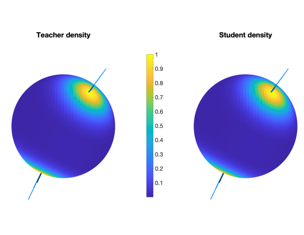
Figure 5: Comparison between the teacher and student density in $d=2$, after training ($n=10^{4},\ N=2\cdot 10^{4},m=62,\alpha=10,p_{R}=0$). The location of the 2 teachers neurons are shown in black, and that of the 64 students neurons in blue.

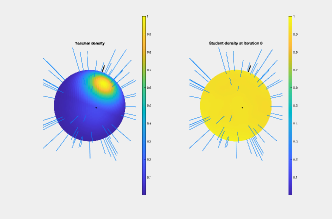
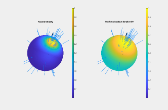
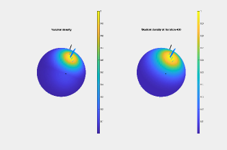
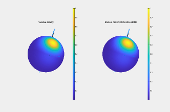
Figure 6: Experiments in $d=2$: Selected frames of the video KLdual_1e4_datapoints_monomodal.mp4 at iterations 0 (top left), 80 (top right), 400 (bottom left) and 40000 (bottom right). The parameters are $d=2,\ m=64,\ p_{R}=0,\ n=10^{4},\ N=2\cdot 10^{4},\ w_{1}^{*}=w_{2}^{*}=-10$. The teacher neurons, shown as black sticks, are almost perpendicular, and hence the teacher distribution is monomodal. The 64 student neurons are shown in blue. The two stages of training mentioned in text are clearly visible.

Figure 7: Experiments in d=2: The evolution of the KL divergence, the score matching metric and the TV norm of the trained measure (i.e., the $\mathcal{F}_{1}$ norm) during training for Algorithm 1 with $\mathcal{X}=\mathbb{S}^{2}$, $m=64$, $p_{R}\in\{0,1,1/60\}$, $s=0.02$, $\alpha=2+10p_{R}$, and (left) $n=10^{3}$, $N=2\cdot 10^{3}$, (right) $n=10^{4}$, $N=2\cdot 10^{4}$. In comparison, the non-parametric kernel density estimator reaches a KL error of $2\cdot 10^{-2}$ for $n=10^{3}$ and $6\cdot 10^{-3}$ for $n=10^{4}$.

Bimodality vs. monomodality in $d=14$. Figure 8 shows the histograms for the cosines of the angles between the samples and each teacher neuron. We see that when the two teacher neurons are at an angle of 2.87 rad (almost opposite), the distribution is bimodal. When they are at an angle of 1.37 rad, the distribution is monomodal.

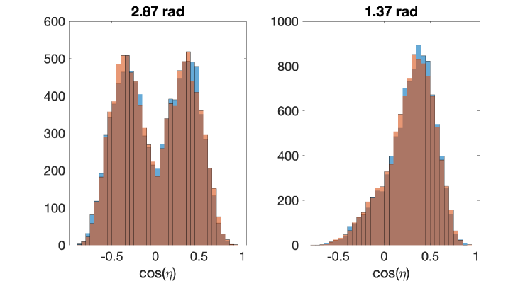
Figure 8: Experiments in d=14: Histograms for the cosines of the angles between each teacher neuron and samples from the target distribution, when the angle between teacher neurons is 2.87 and 1.37 rad.

Comparing different values of $p_{R}$ for $d=14$. In Figure 10 (top, middle), which correspond to the bimodal case with angle 2.87 rad, we observe that the three variants have similar performance but $p_{R}=1/40$ achieves the best metrics, followed very closely by $p_{R}=0$ and $p_{R}=1$ (score matching) a bit behind. Remark that early stopping might be beneficial in terms of the test error; the best test metrics are achieved roughly at the iteration at which the $\mathcal{F}_{1}$ norm of the trained energy reaches the $\mathcal{F}_{1}$ norm of the teacher energy. Interestingly, in the monomodal case with angle 1.37 rad (bottom of Figure 10), the best value for the KL divergence is achieved by $p_{R}=1$ with early stopping, which beats the other two alternatives by a narrow margin. Unlike in the bimodal case, in the monomodal setting the training curves for the three methods display a change of behavior (a bump) slightly after initialization, and before the metrics reach values close to the final ones. This observation seems at odds with the common intuition that monomodal distributions are “easier” to deal with. To assess that the planted model defines a challenging high-dimensional density estimation problem, we consider a kernel density estimator baseline using an RBF kernel projected in the unit sphere. We report the KL divergences obtained in 10, and they are much higher than the EBM ones.

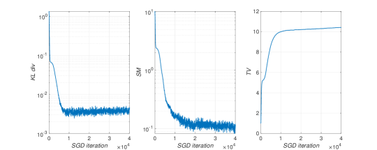
Figure 9: Experiments in $d=2$: Evolution of the KL divergence, score matching and TV norm for the training dynamics of KLdual_1e4_points_monomodal.mp4 and Figure 6.

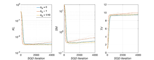
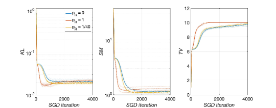
Figure 10: Experiments in d=14: (Top) The evolution of the KL divergence, the score matching metric and the TV norm of the trained measure (i.e., the $\mathcal{F}_{1}$ norm) during training for Algorithm 1 with $\mathcal{X}=\mathbb{S}^{14}$, $m=64$, $p_{R}=0,1,1/40$, $s=0.02$, $\alpha=10+50p_{R}$, $n=10^{3}$, $N=2\cdot 10^{3}$. The plots show the average, maxima and minima over six runs with different training and test samples, initializations and noise realizations, but with the same teacher network with an angle of 2.87 rad between neurons. In comparison, the non-parametric kernel density estimator reaches a KL divergence of $0.18$. (Middle) Same experiments with $n=10^{4}$ and $N=2\cdot 10^{4}$. The non-parametric kernel density estimator reaches a KL divergence of $0.11$. (Bottom) Same experiments with $n=10^{4}$ and $N=2\cdot 10^{4}$, and angle of 1.37 rad between teacher neurons. In comparison, the non-parametric kernel density estimator reaches a KL divergence of $0.15$.

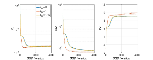
Figure 11: Experiments in $d=14$: Same setting as bottom row of Figure 10 (i.e., angle 1.37 rad), but with $n=10^{5},N=2\cdot 10^{5}$.

In the bottom row of Figure 10, we observe that when the teacher distribution is monomodal, which happens when the teacher neurons are close to perpendicular, the training curves present a “bumpy” shape unlike in the bimodal case. Figure 11 shows plots in the same setting, but with 10 times more training data points. As already observed in Figure 7 and Figure 10, taking larger $n$ improves the relative performance of score matching ($p_{R}=1$) against the other two choices. It is also remarkable that the value of the KL divergence at the end of training in Figure 11 is about $2\cdot 10^{-2}$, which is very similar to the value obtained in the bottom row of Figure 10 despite the increase in $n$. This is at odds with the statistical analysis of Domingo-Enrich et al. [2021], which predicts a decrease of the KL test error as $O(1/\sqrt{n})$ in the case where the approximation error is null. Hence, even though the KL values achieved are low, there is some effect at play which hinders optimization in the monomodal case.

To further understand the “bumpy” curves observed in the monomodal case, we return to experiments in $d=2$, this time with almost perpendicular teacher neurons. The results are shown in Figure 6. We observe similar trends in the curves of Figure 9. In Figure 6, we see that the training occurs in two stages: first the student neurons first concentrate rather quickly near the mode of the teacher distribution: second, they slowly converge toward the teacher neurons. The bump in the KL and SM curves occurs when the first training stage ends and the second one sets in.

These findings seem to suggest an interesting dichotomy: when the two teacher neurons are far away and the distribution is bimodal, sampling is hard but training is easier; when the teacher neurons are closer and the distribution is monomodal, the opposite is true. In a generic situation, both issues may be present. More experiments are required to formulate concrete statements.

References

- Altun and Smola [2006] Y. Altun and A. Smola. Unifying divergence minimization and statistical inference via convex duality. In Learning Theory, pages 139–153. Springer Berlin Heidelberg, 2006.
- Arbel and Gretton [2018] M. Arbel and A. Gretton. Kernel conditional exponential family. In Proceedings of the Twenty-First International Conference on Artificial Intelligence and Statistics, volume 84 of Proceedings of Machine Learning Research, pages 1337–1346. PMLR, 2018.
- Arbel et al. [2019] M. Arbel, A. Korba, A. Salim, and A. Gretton. Maximum mean discrepancy gradient flow. In Advances in Neural Information Processing Systems, volume 32, 2019.
- Bach [2017] F. Bach. Breaking the curse of dimensionality with convex neural networks. Journal of Machine Learning Research, 18(19):1–53, 2017.
- Barron [1993] A. Barron. Universal approximation bounds for superpositions of a sigmoidal function. Information Theory, IEEE Transactions on, 39:930 – 945, 1993.
- Berlinet and Thomas-Agnan [2004] A. Berlinet and C. Thomas-Agnan. Reproducing Kernel Hilbert Space in Probability and Statistics. Springer, 2004.
- Borwein and Zhu [2005] J. Borwein and Q. Zhu. Techniques of Variational Analysis. CMS Books in Mathematics. Springer-Verlag New York, 2005.
- Chen et al. [2020] Z. Chen, G. M. Rotskoff, J. Bruna, and E. Vanden-Eijnden. A dynamical central limit theorem for shallow neural networks, 2020.
- Chizat and Bach [2018] L. Chizat and F. Bach. On the global convergence of gradient descent for over-parameterized models using optimal transport. In Advances in neural information processing systems, pages 3036–3046, 2018.
- Chizat et al. [2018] L. Chizat, G. Peyré, B. Schmitzer, and F.-X. Vialard. Unbalanced optimal transport: Dynamic and kantorovich formulations. Journal of Functional Analysis, 274(11):3090–3123, 2018.
- Cho and Saul [2009] Y. Cho and L. K. Saul. Kernel methods for deep learning. In Advances in Neural Information Processing Systems 22, pages 342–350. Curran Associates, Inc., 2009.
- Dai et al. [2019a] B. Dai, H. Dai, A. Gretton, L. Song, D. Schuurmans, and N. He. Kernel exponential family estimation via doubly dual embedding. In Proceedings of the Twenty-Second International Conference on Artificial Intelligence and Statistics, volume 89 of Proceedings of Machine Learning Research, pages 2321–2330. PMLR, 2019a.
- Dai et al. [2019b] B. Dai, Z. Liu, H. Dai, N. He, A. Gretton, L. Song, and D. Schuurmans. Exponential family estimation via adversarial dynamics embedding. In Advances in Neural Information Processing Systems, volume 32. Curran Associates, Inc., 2019b.
- Dhariwal and Nichol [2021] P. Dhariwal and A. Nichol. Diffusion models beat gans on image synthesis. arXiv preprint arXiv:2105.05233, 2021.
- Domingo-Enrich et al. [2020] C. Domingo-Enrich, S. Jelassi, A. Mensch, G. Rotskoff, and J. Bruna. A mean-field analysis of two-player zero-sum games. In Advances in Neural Information Processing Systems, volume 33, pages 20215–20226. Curran Associates, Inc., 2020.
- Domingo-Enrich et al. [2021] C. Domingo-Enrich, A. Bietti, E. Vanden-Eijnden, and J. Bruna. On energy-based models with overparametrized shallow neural networks. In Proceedings of the 38th International Conference on Machine Learning, volume 139, pages 2771–2782, 2021.
- Du and Mordatch [2019] Y. Du and I. Mordatch. Implicit generation and generalization in energy-based models. In Advances in Neural Information Processing Systems (NeurIPS), 2019.
- Dudík et al. [2007] M. Dudík, S. J. Phillips, and R. E. Schapire. Maximum entropy density estimation with generalized regularization and an application to species distribution modeling. J. Mach. Learn. Res., 8:1217–1260, 2007.
- Dunford and Schwartz [1958] N. Dunford and J. T. Schwartz. Linear operators. Part I, General theory. Pure and applied mathematics (Interscience series). Interscience, 1958.
- Dziugaite et al. [2015] G. K. Dziugaite, D. M. Roy, and Z. Ghahramani. Training generative neural networks via maximum mean discrepancy optimization. UAI, 2015.
- E and Wojtowytsch [2020] W. E and S. Wojtowytsch. On the banach spaces associated with multi-layer relu networks: Function representation, approximation theory and gradient descent dynamics, 2020.
- E et al. [2019] W. E, C. Ma, and L. Wu. A priori estimates of the population risk for two-layer neural networks. Communications in Mathematical Sciences, 17:1407–1425, 01 2019.
- Ekeland and Temam [1999] I. Ekeland and R. Temam. Convex analysis and variational problems. Philadelphia, Pa: Society for Industrial and Applied Mathematics, 1999.
- Gibbs [2010] J. W. Gibbs. Elementary Principles in Statistical Mechanics: Developed with Especial Reference to the Rational Foundation of Thermodynamics. Cambridge Library Collection - Mathematics. Cambridge University Press, 2010.
- Gretton et al. [2007] A. Gretton, K. M. Borgwardt, M. Rasch, B. Schölkopf, and A. J. Smola. A kernel method for the two-sample-problem. In Advances in neural information processing systems, pages 513–520, 2007.
- Gretton et al. [2012] A. Gretton, K. M. Borgwardt, M. J. Rasch, B. Schölkopf, and A. Smola. A kernel two-sample test. Journal of Machine Learning Research, 13(25):723–773, 2012.
- Heusel et al. [2017] M. Heusel, H. Ramsauer, T. Unterthiner, B. Nessler, and S. Hochreiter. GANs trained by a two time-scale update rule converge to a local Nash equilibrium. In Advances in Neural Information Processing Systems, pages 6626–6637, 2017.
- Hinton [2002] G. E. Hinton. Training products of experts by minimizing contrastive divergence. Neural Comput., 14(8):1771–1800, 2002.
- Ho et al. [2020] J. Ho, A. Jain, and P. Abbeel. Denoising diffusion probabilistic models. In Advances in Neural Information Processing Systems, volume 33. Curran Associates, Inc., 2020.
- Hyvärinen [2005] A. Hyvärinen. Estimation of non-normalized statistical models by score matching. Journal of Machine Learning Research, 6(24):695–709, 2005.
- Jaynes [1957] E. T. Jaynes. Information theory and statistical mechanics. Phys. Rev., 106:620–630, May 1957.
- Jolicoeur-Martineau et al. [2020] A. Jolicoeur-Martineau, R. Piché-Taillefer, R. T. d. Combes, and I. Mitliagkas. Adversarial score matching and improved sampling for image generation. arXiv preprint arXiv:2009.05475, 2020.
- Kadkhodaie and Simoncelli [2020] Z. Kadkhodaie and E. P. Simoncelli. Solving linear inverse problems using the prior implicit in a denoiser. arXiv preprint arXiv:2007.13640, 2020.
- Kneser [1952] H. Kneser. Sur un theoreme fondamentale de la theorie des jeux. C. R. Acad. Sci. Paris, 234:2418–2420, 1952.
- LeCun et al. [2006] Y. LeCun, S. Chopra, R. Hadsell, M. Ranzato, and F. Huang. A tutorial on energy-based learning. 2006.
- Li et al. [2017] C.-L. Li, W.-C. Chang, Y. Cheng, Y. Yang, and B. Poczos. Mmd gan: Towards deeper understanding of moment matching network. In Advances in Neural Information Processing Systems, volume 30, 2017.
- Li et al. [2015] Y. Li, K. Swersky, and R. Zemel. Generative moment matching networks. In ICML, 2015.
- Lin et al. [2020] T. Lin, C. Jin, and M. I. Jordan. On gradient descent ascent for nonconvex-concave minimax problems. In Proceedings of the 37th International Conference on Machine Learning, 2020.
- McKean [1967] H. McKean. A class of markov processes associated with nonlinear parabolic equations. Proceedings of the National Academy of Sciences of the United States of America, 56:1907–11, 01 1967.
- Mei et al. [2018] S. Mei, A. Montanari, and P.-M. Nguyen. A mean field view of the landscape of two-layer neural networks. Proceedings of the National Academy of Sciences, 115(33):E7665–E7671, 2018.
- Mohri et al. [2012] M. Mohri, A. Rostamizadeh, and A. Talwalkar. Foundations of Machine Learning. The MIT Press, 2012.
- Neumann [1928] J. v. Neumann. Zur theorie der gesellschaftsspiele. Mathematische annalen, 100(1):295–320, 1928.
- Posner [1975] E. C. Posner. Random coding strategies for minimum entropy. IEEE Transations on Information Theory, 21(4):388–391, 1975.
- Rahimi and Recht [2008] A. Rahimi and B. Recht. Random features for large-scale kernel machines. In J. C. Platt, D. Koller, Y. Singer, and S. T. Roweis, editors, Advances in Neural Information Processing Systems 20, pages 1177–1184. Curran Associates, Inc., 2008.
- Ranzato et al. [2007] M. Ranzato, C. Poultney, S. Chopra, et al. Efficient learning of sparse representations with an energy-based model. 2007.
- Rotskoff and Vanden-Eijnden [2018] G. M. Rotskoff and E. Vanden-Eijnden. Neural networks as interacting particle systems: Asymptotic convexity of the loss landscape and universal scaling of the approximation error. arXiv preprint arXiv:1805.00915, 2018.
- Rotskoff et al. [2019] G. M. Rotskoff, S. Jelassi, J. Bruna, and E. Vanden-Eijnden. Global convergence of neuron birth-death dynamics. In Proceedings of the 36th International Conference on International Conference on Machine Learning, Long Beach, CA, USA, 2019.
- Roux and Bengio [2007] N. L. Roux and Y. Bengio. Continuous neural networks. In Proceedings of the Eleventh International Conference on Artificial Intelligence and Statistics, volume 2 of Proceedings of Machine Learning Research, pages 404–411, San Juan, Puerto Rico, 21–24 Mar 2007.
- Ruelle [1969] D. Ruelle. Statistical mechanics: Rigorous results. W.A. Benjamin, 1969.
- Santambrogio [2017] F. Santambrogio. Euclidean, metric, and Wasserstein gradient flows: an overview. Bulletin of Mathematical Sciences, 7(1):87–154, 2017.
- Sion [1958] M. Sion. On general minimax theorems. Pacific J. Math., 8(1):171–176, 1958.
- Sirignano and Spiliopoulos [2019] J. Sirignano and K. Spiliopoulos. Mean field analysis of neural networks: A central limit theorem. Stochastic Processes and their Applications, 2019.
- Song and Ermon [2019] Y. Song and S. Ermon. Generative modeling by estimating gradients of the data distribution. arXiv preprint arXiv:1907.05600, 2019.
- Song and Ermon [2020] Y. Song and S. Ermon. Improved techniques for training score-based generative models. In Advances in Neural Information Processing Systems, 2020.
- Song and Kingma [2021] Y. Song and D. P. Kingma. How to train your energy-based models, 2021.
- Song et al. [2021] Y. Song, J. Sohl-Dickstein, D. P. Kingma, A. Kumar, S. Ermon, and B. Poole. Score-based generative modeling through stochastic differential equations. In International Conference on Learning Representations (ICLR 2021), 2021.
- Sutherland et al. [2018] D. J. Sutherland, H. Strathmann, M. Arbel, and A. Gretton. Efficient and principled score estimation with nyström kernel exponential families. In Proceedings of the Twenty-First International Conference on Artificial Intelligence and Statistics, volume 84 of Proceedings of Machine Learning Research, pages 652–660. PMLR, 2018.
- Sznitman [1991] A.-S. Sznitman. Topics in propagation of chaos. In P.-L. Hennequin, editor, Ecole d’Eté de Probabilités de Saint-Flour XIX — 1989, pages 165–251, Berlin, Heidelberg, 1991. Springer Berlin Heidelberg.
- Tieleman [2008] T. Tieleman. Training restricted boltzmann machines using approximations to the likelihood gradient. In Proceedings of the 25th International Conference on Machine Learning, ICML ’08. Association for Computing Machinery, 2008.
- Tieleman and Hinton [2009] T. Tieleman and G. Hinton. Using fast weights to improve persistent contrastive divergence. In Proceedings of the 26th Annual International Conference on Machine Learning, ICML ’09. Association for Computing Machinery, 2009.
- Vincent [2011] P. Vincent. A connection between score matching and denoising autoencoders. Neural Computation, 23(7), 2011.
- Wainwright and Jordan [2008] M. Wainwright and M. Jordan. Graphical models, exponential families, and variational inference. Foundations and Trends in Machine Learning, 1:1–305, 01 2008.
- Xie et al. [2016] J. Xie, Y. Lu, S.-C. Zhu, and Y. Wu. A theory of generative convnet. In Proceedings of The 33rd International Conference on Machine Learning, volume 48 of Proceedings of Machine Learning Research. PMLR, 2016.
- Xie et al. [2017] J. Xie, S. Zhu, and Y. Wu. Synthesizing dynamic patterns by spatial-temporal generative convnet. In IEEE Conference on Computer Vision and Pattern Recognition (CVPR), 2017.