Spatial relative equilibria and periodic solutions of the Coulomb $(n+1)$-body problem

Abstract

We study a classical model for the atom that considers the movement of $n$ charged particles of charge $-1$ (electrons) interacting with a fixed nucleus of charge $\mu>0$. We show that two global branches of spatial relative equilibria bifurcate from the $n$-polygonal relative equilibrium for each critical values $\mu=s_{k}$ for $k\in[2,...,n/2]$. In these solutions, the $n$ charges form $n/h$-groups of regular $h$-polygons in space, where $h$ is the greatest common divisor of $k$ and $n$. Furthermore, each spatial relative equilibrium has a global branch of relative periodic solutions for each normal frequency satisfying some nonresonant condition. We obtain computer-assisted proofs of existence of several spatial relative equilibria on global branches away from the $n$-polygonal relative equilibrium. Moreover, the nonresonant condition of the normal frequencies for some spatial relative equilibria is verified rigorously using computer-assisted proofs.

AMS Subject Classification: 70F10, 65G40, 47H11, 34C25, 37G40

Keywords: Coulomb potential, N-body problem, relative equilibria, periodic solutions

1 Introduction

The Thomson problem is a classical model to study a configuration of $n$ electrons, constrained to the unit sphere, that repel each other with a force given by Coulomb’s law. Thomson posed the problem in 1904 as an atomic model, later called the plum pudding model [13]. Without loss of generality we can assume that the elementary charge of an electron is $e=-1$, its mass is $m=1$, and the Coulomb constant is $1$. We wish to analyze another classical model for the atom that considers the movement of $n$ charged particles with negative charge $-1$ (electrons) interacting with a fixed nucleus with positive charge $\mu$. Since electrons and protons have equal charges with different signs, for a non-ionized atom we consider that $\mu=n$. By supposing that the gravitational forces are smaller than Coulomb’s forces, the system of equations describing the movement of the charges is

$$\ddot{q}_{j}=-\mu\frac{q_{j}}{\left\|q_{j}\right\|^{3}}+\sum_{i=0~{}(i\neq j)}^{n-1}\frac{q_{j}-q_{i}}{\left\|q_{j}-q_{i}\right\|^{3}},\qquad q_{j}\in\mathbb{R}^{3},\qquad j=0,...,n-1,$$ (1)

where the first term of the force represents the interaction with the fixed nucleus.

This problem is referred to as the charged $(n+1)$-body problem [8, 1], the $n$-electron atom problem [4] and the Coulomb $(n+1)$-body problem [6] (and the references therein). An interesting feature of this problem is the existence of spatial relative equilibria, in contrast to the $n$-body problem where all relative equilibria must be planar [1]. In this paper we investigate the existence of bifurcations of spatial relative equilibria arising from the polygonal relative equilibrium. The existence of bifurcations of spatial central configurations arising from planar configurations has been investigated previously in [16].

Specifically, we study equation (1) in rotating coordinates $u_{j}$ with frequency $\sqrt{\omega}$, $q_{j}(t)=e^{\sqrt{\omega}t\bar{J}}u_{j}(t)$, where $\bar{J}=J\oplus 0$ and $J$ is the standard symplectic matrix in $\mathbb{R}^{2}$. The starting solution of our study is the planar unitary polygon $u=a$, which is an equilibrium of the equations in a rotating frame with $\omega=\mu-s_{1}>0$, where

$$s_{k}\,\overset{\mbox{\tiny{\raisebox{0.0pt}[0.0pt][0.0pt]{def}}}}{=}\,\frac{1}{4}\sum_{j=1}^{n-1}\frac{\sin^{2}(kj\pi/n)}{\sin^{3}(j\pi/n)}\text{,\qquad}k=0,...,n-1.$$

In Theorem 2.2 we prove that for each $k\in[2,n/2]\cap\mathbb{N}$, there are two global bifurcations of stationary solutions (in rotating frame) from the trivial solution $u={a}$ at $\mu=s_{k}$. Furthermore, each solution in the families is a spatial relative equilibrium where the $n$ charges form $n/h$-groups of regular $h$-polygons in the space, where $h$ is the greatest common divisor of $k$ and $n$ (this fact can be observed in the numerical computations in Figures 1, 2, 3 and 4). By global bifurcation we mean that the bifurcation forms a connected component that either goes to other relative equilibria, ends in a collision configuration or its norm goes to infinity. The global property is proved using Brouwer degree along the lines of the result in [7], which treats the bifurcation of relative equilibria from the unitary polygon in the $n$-body problem.

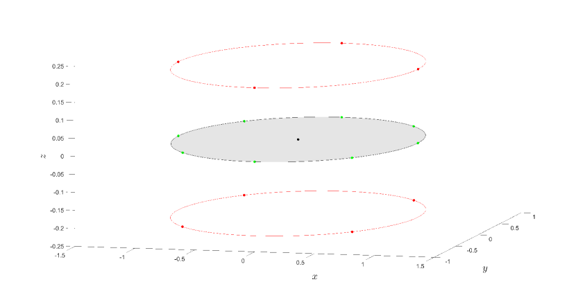
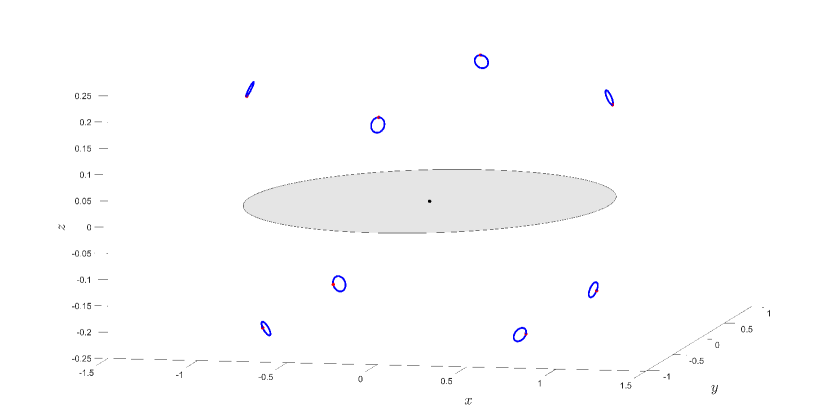
Figure 1: Left: A relative equilibrium solutions for $n=8$ and $k=4$ in the first family, whose existence has been obtained using a computer-assisted proof (together with tight error bounds). Right: The first order expansion of the family of periodic solutions arising from the relative equilibrium in a rotating frame.

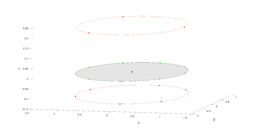
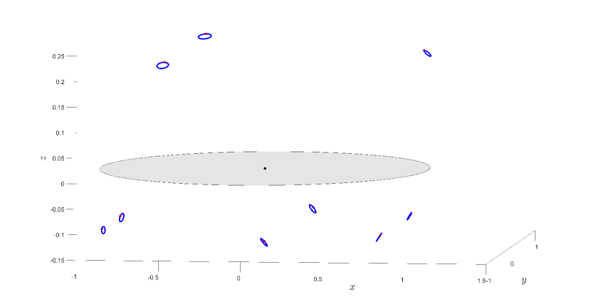
Figure 2: Left: A relative equilibrium solutions for $n=9$ and $k=3$ in the first family, whose existence has been obtained using a computer-assisted proof (together with tight error bounds). Right: The first order expansion of the family of periodic solutions arising from the relative equilibrium in a rotating frame.

In the rotating frame, the linearized system at a spatial relative equilibrium exhibits many periodic solutions (normal modes). In the present paper, we prove the persistence of these periodic solutions in the nonlinear system (see Theorem 2.5). These solutions are referred to as nonlinear normal modes or Lyapunov families. In the inertial frame they are known as relative periodic solutions and correspond to periodic or quasiperiodic solutions. Furthermore, we prove the global property, which in the present context means that a family of periodic solutions, represented by a continuous branch $\mathcal{C}$ in the space of frequencies and $2\pi$-periodic paths, is not compact or comes back to another bifurcation point. The non-compactness of $\mathcal{C}$ implies that either the norm or period of the solutions from $\mathcal{C}$ goes to infinity or $\mathcal{C}$ ends in a collision orbit. The proof of the global property is akin to the proof in [7] regarding the existence of periodic solutions from the polygonal relative equilibrium $a$, and is obtained by means of the $SO(2)\times S^{1}$-equivariant degree developed in [10].

The result of Theorem 2.5 holds when some non-resonance assumptions (Definition 2.4) on the normal frequencies of the spatial relative equilibrium are satisfied. A main contribution of the present paper is the implementation of computer-assisted proofs to validate global branches of spatial relative equilibria and also the non-resonance assumption, which is required to obtain the existence of families of periodic solutions arising from them. In Section 3, we present the general approach (a Newton-Kantorovich type theorem, see Theorem 3.1) used to obtain the different computer-assisted proofs. This theorem is used to validate the spatial relative equilibria (in Section 3.1) and its normal frequencies (in Section 3.2) to verify the conditions of Theorem 2.5. Figures 1 and 2 contain an example of spatial relative equilibria whose existence has been obtained using a computer-assisted proof (together with tight error bounds) and for which the non-resonance condition has been rigorously verified. Similar computer-assisted proofs were carried on for each (non black) point in Figures 3 and 4.

2 Existence of periodic solutions arising from spatial relative equilibria

We assume that: the gravitational forces are much smaller than Coulomb’s forces, the charge in the center is $\mu>0$, the $n$ charges have charge $-1$, the mass of the charges is $m=1$ and the Coulomb constant is $\kappa=1$. We also assume that the position of the central charge is fixed at the center and the positions of the $n$ charges are determined by $q(t)=(q_{0}(t),...,\,q_{n-1}(t))$ with $q_{j}(t)\in\mathbb{R}^{3}$ for $j=0,...,n-1$. Under these assumptions, the system satisfies the Newtonian equation

$$\ddot{u}(t)=\nabla U(q(t)),$$ (2)

where $U(q)$ is the potential energy given by

$$U(q)\,\overset{\mbox{\tiny{\raisebox{0.0pt}[0.0pt][0.0pt]{def}}}}{=}\,\sum_{j=0}^{n-1}\frac{\mu}{\|q_{j}\|}-\sum_{i<j}\frac{1}{\|q_{j}-q_{i}\|},$$

where the first term represents the interaction with the fixed center.

Let $\bar{J}=J\oplus 0$, where $J$ is the standard symplectic matrix in $\mathbb{R}^{2}$. In rotating coordinates, $q_{j}(t)=e^{\sqrt{\omega}t\bar{J}}u_{j}(t)$, the system of equations becomes $\ddot{u}_{j}+2\sqrt{\omega}\bar{J}\dot{u}_{j}=\nabla_{u_{j}}V(u)$, where $V$ is the augmented potential

$$V(u)=\frac{\omega}{2}\sum_{j=0}^{n-1}\left\|\bar{I}u_{j}\right\|^{2}+\sum_{j=0}^{n-1}\frac{\mu}{\left\|u_{j}\right\|}-\sum_{i<j}\frac{1}{\left\|u_{j}-u_{i}\right\|}\text{,}$$

where $\bar{I}=-\bar{J}^{2}=1\oplus 1\oplus 0$. Let $u=(u_{0},...,u_{n-1})$ and $\mathcal{\bar{J}}=\bar{J}\oplus...\oplus\bar{J}$, the system of equation reads

$$\ddot{u}+2\sqrt{\omega}\mathcal{\bar{J}}\dot{u}=\nabla V(u)\text{.}$$ (3)

Let $S_{n}$ be the group of permutations of $\{0,1,...,n-1\}$ and $D_{n}$ be the subgroup generated by the permutations $\zeta(j)=j+1$ and $\kappa(j)=n-j$ mod $n$. We define the action of $\gamma\in S_{n}$ in $\mathbb{R}^{3n}$ as

$$\rho(\gamma)(u_{0},u_{1},...,u_{n-1})=(u_{\gamma(0)},u_{\gamma(1)},...,u_{\gamma(n-1)}).$$ (4)

Notice that this is a left action only if the product on $S_{n}$ is defined according to the opposite convention that $\sigma_{1}\sigma_{2}\,\overset{\mbox{\tiny{\raisebox{0.0pt}[0.0pt][0.0pt]{def}}}}{=}\,\sigma_{2}\circ\sigma_{1}$. Clearly the potential $V$ is $S_{n}$-invariant. On the other hand, while the potential $U(u)$ is $O(3)$-invariant, the potential $V(u)$ is only invariant under the action of the normalizer $O(2)\times\mathbb{Z}_{2}$ of $SO(2)\subset O(3)$.

We conclude that $V(u)$ is $G$-invariant with

$$G\,\overset{\mbox{\tiny{\raisebox{0.0pt}[0.0pt][0.0pt]{def}}}}{=}\,S_{n}\times O(2)\times\mathbb{Z}_{2}.$$

The explicit action of the elements $\theta,\kappa_{y}\in O(2)$ and $\kappa_{z}\in\mathbb{Z}_{2}$ in the components of $u$ is given by

$$\theta u_{j}=e^{-\mathcal{\bar{J}}\theta}u_{j},\qquad\kappa_{y}u_{j}=R_{y}u_{j},\qquad\kappa_{z}u_{j}=R_{z}u_{j},$$

where

$$R_{y}=1\oplus-1\oplus 1,\qquad R_{z}=1\oplus 1\oplus-1.$$

2.1 The polygonal relative equilibrium

The polygon $a=(a_{0},...,a_{n-1})$, where

$$a_{j}=\left(e^{ij\zeta},0\right)\in\mathbb{C\times R},\qquad\zeta\,\overset{\mbox{\tiny{\raisebox{0.0pt}[0.0pt][0.0pt]{def}}}}{=}\,2\pi/n,$$

is a critical point of $V(u;\omega)$ for $\omega=\mu-s_{1}>0$. This follows from the identity

$$\nabla_{u_{j}}V(a)=\omega a_{j}-\mu a_{j}+\sum_{i=0~{}(i\neq j)}^{n-1}\frac{a_{j}-a_{i}}{\left\|a_{j}-a_{i}\right\|^{3}}=a_{j}\left(\omega-\mu+s_{1}\right),$$

where we have used that

$$\sum_{i=0~{}(i\neq j)}^{n-1}\frac{a_{j}-a_{i}}{\left\|a_{j}-a_{i}\right\|^{3}}=a_{j}\sum_{i=0~{}(i\neq j)}^{n-1}\frac{1-e^{ij\zeta}}{\left\|1-e^{ij\zeta}\right\|^{3}}=a_{j}\frac{1}{4}\sum_{j=1}^{n-1}\frac{1}{\sin(j\pi/n)}=a_{j}s_{1}\text{.}$$

2.2 Bifurcation of spatial relative equilibria

Hereafter we assume that $\omega=\mu-s_{1}$ and we denote the dependence of the potential $V$ in the parameter $\mu$ as $V(u;\mu)$. Thus the polygon $u=a$ is a trivial solution of $\nabla V(u;\mu)=0$ with isotropy group $G_{a}$ generated by

$$\tilde{\zeta}=\left(\zeta,\zeta,e\right),\qquad\tilde{\kappa}_{y}=\left(\kappa,\kappa_{y},e\right),\qquad\tilde{\kappa}_{z}=\left(e,e,\kappa_{z}\right)\in S_{n}\times O(2)\times\mathbb{Z}_{2},$$

where $e$ represents the identity element. As a consequence of the continuous action of $SO(2)$, the orbit of the polygonal equilibrium $a$ is one dimensional. Thus the generator of the $SO(2)$-orbit of $a$ is $-\bar{\mathcal{J}}a$, which belongs to the kernel of $D^{2}V(u)$.

Given that $G_{a}$ fixes $a$, then $D^{2}V(a)$ is $G_{a}$-equivariant and, by Schur’s lemma, it has the same eigenvalue in each irreducible representations under the action of $G_{a}$. The spatial irreducible representations of $G_{a}$ are obtained in section “8.4. The problem of $n$-charges” in the paper [8]. Define $V_{k}$ as the subspace generated by

$$v_{k}=\left(v_{k}^{0},,...,v_{k}^{n-1}\right)\in\mathbb{R}^{3n},$$

where $v_{k}^{j}=(0,0,\cos jk\zeta)$ for $k\in\left[0,n/2\right]\cap\mathbb{N}$ and $v_{k}^{j}=(0,0,\sin jk\zeta)$ for $k\in(n/2,n-1]\cap\mathbb{N}$, then the irreducible $G_{a}$-representations are given by $V_{k}$ for $k=0,n/2$ and $V_{k}\oplus V_{n-k}$ for $k\in[1,n/2)\cap\mathbb{N}$.

Specifically, using the isomorphism

$$av_{k}+bv_{n-k}\in V_{k}\oplus V_{n-k}\rightarrow a+ib\in\mathbb{C},$$

the action of $\tilde{\zeta},\tilde{\kappa}_{y},\tilde{\kappa}_{z}\in G_{a}$ in $z=a+ib\in\mathbb{C}$ is given by

$$\tilde{\zeta}z=e^{ik\zeta}z,\qquad\tilde{\kappa}_{y}z=\bar{z},\qquad\tilde{\kappa}_{z}z=-z.$$ (5)

For $k=0,n/2$ the action in $V_{k}\simeq\mathbb{R}$ is the same as before but with $z\in\mathbb{R}$. For instance, for $k\in(0,n/2)\cap\mathbb{N}$ we have that

$$\tilde{\zeta}\left(av_{k}+bv_{n-k}\right) =e^{-\mathcal{\bar{J}}\zeta}\zeta\cdot\left(av_{k}+bv_{n-k}\right)$$

$$=\left\{\left(0,0,a\cos(jk+k)\zeta-b\sin(jk+k)\zeta\right)\right\}_{j=1}^{n}$$

$$=\left(a\cos k\zeta-b\sin k\zeta\right)v_{k}+\left(b\cos k\zeta+a\sin k\zeta\right)v_{n-k}.$$

Hence, we obtain that

$$\tilde{\zeta}z=\left(a\cos k\zeta-b\sin k\zeta\right)+i\left(b\cos k\zeta+a\sin k\zeta\right)=e^{ik\zeta}z.$$

In section “8.4. The problem of $n$-charges” in the paper [8] is proven that the eigenvalue of Hessian $D^{2}V(a)$ in each irreducible representation $V_{k}$ for $k=0,n/2$ and $V_{k}\oplus V_{n-k}$ is $-\mu+s_{k}$. For sake of completeness we present a short proof of this fact. For $k\in\{0,...,n-1\}$, we define $T_{k}:\mathbb{R}\rightarrow W_{k}$ as

$$T_{k}(w) =(0,0,n^{-1/2}e^{ik\zeta}w,...,0,0,n^{-1/2}e^{nik\zeta}w)\text{ with }$$

$$W_{k} =\{(0,0,e^{ik\zeta}w,...,0,0,e^{nik\zeta}w)\in\mathbb{C}^{3n}:w\in\mathbb{R}\}\text{.}$$

Since $W_{k}=V_{k}\oplus iV_{n-k}$, the result follows from the invariance of the subspaces $W_{k}$ of $D^{2}V(a)$ with the following computation.

Proposition 2.1.

For $k\in\{0,...,n-1\}$, we have

$$D^{2}V(a)T_{k}(w)=T_{k}(\left(-\mu+s_{k}\right)w).$$

Proof.

Let $\mathcal{A}_{ij}$ be the $3\times 3$ minor blocks of the Hessian $D^{2}V(a)=(\mathcal{A}_{ij})_{ij=1}^{n}$. The fact that $a$ is a planar configuration implies that the matrices $\mathcal{A}_{ij}$ are block diagonal

$$\mathcal{A}_{ij}=diag(A_{ij},a_{ij})\text{,}$$

where $A_{ij}$ is a $2\times 2$ matrix. For our purpose we only need to compute the numbers $a_{ij}$. Let $d_{ij}=\left|u_{i}-u_{j}\right|$ be the distance between $u_{i}=(x_{i},y_{i},z_{i})$ and $u_{j}=(x_{j},y_{j},z_{j})$. For $i\neq j$ we have that $\partial_{z_{i}}(d_{ij}^{-1})=-\partial_{z_{j}}(d_{ij}^{-1})$ and

$$a_{ij}=-\partial_{z_{j}}\partial_{z_{i}}d_{ij}^{-1}|_{u=a}=\partial_{z_{i}}^{2}d_{ij}^{-1}|_{u=a}=-d_{ij}^{-3}|_{u=a}=-\left(2\sin((i-j)\zeta/2)\right)^{-3}\text{.}$$ (6)

For $i=j$ the number $a_{ii}$ satisfies

$$a_{ii}=\partial_{z_{i}}^{2}\left(\frac{\mu}{\left\|u_{j}\right\|}\right)_{u_{j}=a_{j}}-\sum_{j=0~{}(j\neq i)}^{n-1}\left(\partial_{z_{i}}^{2}d_{ij}^{-1}\right)_{u_{j}=a_{j}}=-\mu-\sum_{j=0~{}(j\neq i)}^{n-1}a_{ij}\text{.}$$

Now we need to denote to the component $w_{i}\in\mathbb{C}^{3}$ of the vector $w=(w_{0},...,w_{n-1})\in\mathbb{C}^{3n}$ as $[w]_{i}=w_{i}$. From the definitions we have that

$$[D^{2}V(a)T_{k}(w)]_{l}=\left(0,0,n^{-1/2}\sum_{j=0}^{n-1}a_{lj}e^{ijk\zeta}w\right)\text{.}$$

Since $a_{lj}=a_{0(j-l)}$ with $(j-l)\in\{0,...,n-1\}$ modulus $n$. From the equality $a_{lj}e^{ijk\zeta}=e^{ilk\zeta}\left(a_{0(j-l)}e^{i(j-l)k\zeta}\right)$ we have that

$$[D^{2}V(a)T_{k}(w)]_{l}=\left(0,0,n^{-1/2}e^{ilk\zeta}b_{k}w\right)=\left[T_{k}(b_{k}w)\right]_{l}\text{,}$$

where

$$b_{k}=\sum_{j=0}^{n-1}a_{0j}e^{ijk\zeta}=-\mu+\sum_{j=1}^{n-1}\left(e^{ijk\zeta}-1\right)a_{0j}\text{,}$$

because $a_{00}=-\mu-\sum_{j=0}^{n-1}a_{0j}$. Finally, using (6), we obtain that

$$\sum_{j=1}^{n-1}\left(e^{ijk\zeta}-1\right)a_{0j}=\sum_{j=1}^{n-1}\frac{2\sin^{2}(kj\zeta/2)}{2^{3}\sin^{3}(j\zeta/2)}=s_{k}\text{.}$$

∎

According to [8], for $k\in[2,n/2)$, the Hessian $D^{2}V(u;s_{k})$ has no additional zero-eigenvalues to the double zero-eigenvalue corresponding to the subspace $V_{k}\oplus V_{n-k}$ and the simple zero-eigenvalue corresponding to the generator of the $xy$-rotations $-\bar{\mathcal{J}}a$. That is,

$$\ker D^{2}V(a;s_{k})=V_{k}\oplus V_{n-k}\oplus\bar{\mathcal{J}}{a}.$$

In order to prove the existence of solutions $\nabla V(u;\mu)=0$ bifurcating from the trivial solution $u=a$ when the parameter $\mu$ crosses $s_{k}$, we consider the fixed point spaces of two subgroups

$$H_{1}=\mathbb{Z}_{2}\left(\tilde{\kappa}_{y}\right),\qquad H_{2}=\mathbb{Z}_{2}\left(\tilde{\kappa}_{y}\kappa_{z}\right).$$

That is, let $\nabla V^{H_{j}}:Fix(H_{j})\rightarrow Fix(H_{j})$ be the restriction of $\nabla V$ to the fixed point space of $H_{j}$ for $j=1,2$, we will show that the restricted maps $\nabla V^{H_{j}}$ for $j=1,2$ have the advantage that the zero-eigenvalue $-\bar{\mathcal{J}}a$ is not present in $D^{2}V^{H_{j}}$ and that the double zero-eigenvalue $-\mu+s_{k}$ becomes simple.

The fixed point space of $\mathbb{R}^{3n}$ under the action of $H_{1}$ satisfies the symmetries

$$u_{0}=R_{y}u_{0},\qquad u_{n/2}=R_{y}u_{n/2},\qquad u_{j}=R_{y}u_{n-j},$$ (7)

and of $H_{2}$

$$u_{0}=R_{z}R_{y}u_{0},\qquad u_{n/2}=R_{z}R_{y}u_{n/2},\qquad u_{j}=R_{z}R_{y}u_{n-j}\text{.}$$ (8)

Theorem 2.2.

For each $k\in[2,n/2]\cap\mathbb{N}$, there are two global bifurcations of solutions of $\nabla V(u;\mu)=0$ from the trivial solution $u={a}$ at $\mu=s_{k}$, one denoted by $\mathfrak{F}_{1}^{k}$ with symmetries (7) and another denoted by $\mathfrak{F}_{2}^{k}$ with symmetries (8). Furthermore, the relative equilibria in both families are formed by $n/h$-groups of regular $h$-polygons, where $h$ is the greatest common divisor of $k$ and $n$.

Proof.

We look for bifurcation of solutions of $\nabla V^{H_{1}}(u;\mu)=0$ from the trivial solution $u=a$ at $\mu=s_{k}$. Using that $\ker D^{2}V(a;s_{k})=V_{k}\oplus V_{n-k}\oplus\bar{\mathcal{J}}{a}$, it is easy to see that $v^{n-k}\in V_{n-k}$ and $\bar{\mathcal{J}}{a}$ do not satisfy the symmetry (7), which implies that they do not belong to $Fix(H_{1})$. Thus the kernel of $D^{2}V^{H_{1}}({a};s_{k})$ is one dimensional and generated by $v^{k}\in V_{k}$. The eigenvalue $-\mu+s_{k}$ corresponding to the eigenvector $v^{k}\in V_{k}$ crosses zero at $\mu=s_{k}$. Using Brouwer degree as in section “3. Bifurcation theorem” in [7], we can prove the existence of a global bifurcation of solutions of $\nabla V^{H_{1}}(u;\mu)=0$ from the trivial solution $u={a}$ at $\mu=s_{k}$. Furthermore, since $\tilde{\zeta}^{n/h}$ leaves the subspace $V_{k}$ fixed, because $\tilde{\zeta}^{n/h}z=\left(e^{ik2\pi/n}\right)^{n/h}z=z$ according to (5), then the family of solutions $\mathfrak{F}_{1}^{k}$ arising from $\mu=s_{k}$ is fixed by the group $\mathbb{\tilde{Z}}_{h}$ generated by $\tilde{\zeta}^{n/h}$. This implies that the solution is formed by $n/h$-polygons (see [7] for details). The proof in the case $k=n/2$ and $H_{2}$ is analogous, the only key difference is that

$$\ker D^{2}V^{H_{2}}(a;s_{k})=\ker D^{2}V(a;s_{k})\cap Fix(H_{2})=V_{n-k},$$

because $v^{k}\in V_{k}$ and $\bar{\mathcal{J}}{a}$ do not satisfy the symmetry (8), and they do not belong to $Fix(H_{2})$. ∎

The polygon $a$ is a relative equilibrium only when $\omega=\mu-s_{1}>0$, which requires that $\mu>s_{1}$. In a slightly different context it was noticed by R. Moeckel [15] that the condition $\mu=n>s_{1}$ holds only for $n<473$. An interesting consequence of this fact is that for a non-ionized atom the $n$-polygon is a relative equilibrium only for an atomic number less than $473$. We obtain numerically the additional inequalities $s_{1}<n<s_{2}$ for $n=3$ and $n\geq 12$, $s_{2}<n<s_{3}$ for $n=4,5,8,9,10,11$ and $s_{3}<n<s_{4}$ for $n=6,7$. Since the bifurcations of relative equilibria arising from the polygons at $\mu=s_{k}$ are subcritical, for instance, one can deduce from these inequalities that it is unlikely to find a relative equilibrium with $\mu=n$ in the bifurcation from $s_{1}$ for the cases $n=4,...,11$.

2.3 Periodic solutions arising from spatial relative equilibria

Now we turn the attention to the analysis of non-trivial $2\pi/\nu$-periodic solutions of (3) arising from a spatial relative equilibrium $(u_{0};\mu_{0})$, which for the present paper belongs to the families $\mathfrak{F}_{1}^{k}$ or $\mathfrak{F}_{2}^{k}$. For the validation of the hypotheses necessary to obtain the periodic solutions we will use the computer-assisted proof technique of Section 3. These hypotheses are easier to verify in the equivalent system

$$\begin{pmatrix}\dot{u}\\ \dot{v}\end{pmatrix}=\begin{pmatrix}v\\ -2\sqrt{\mu-s_{1}}\mathcal{\bar{J}}v+\nabla V(u;\mu)\end{pmatrix}.$$ (9)

The linearization of equation (9) at a spatial relative equilibrium $(u_{0};\mu_{0})$ is

$$\binom{\dot{u}}{\dot{v}}=L(u_{0};\mu_{0})\binom{u}{v},\qquad L(u_{0};\mu_{0})\,\overset{\mbox{\tiny{\raisebox{0.0pt}[0.0pt][0.0pt]{def}}}}{=}\,\left(\begin{array}[]{cc}0&I\\ D^{2}V(u_{0};\mu)&-2\sqrt{\mu_{0}-s_{1}}\mathcal{\bar{J}}\end{array}\right).$$

Notice that $\lambda$ is an eigenvalue of $L(u_{0};\mu_{0})$ with eigenvector $(u,v)$ if and only if $v=\lambda u$ and

$$-2\sqrt{\mu_{0}-s_{1}}\mathcal{\bar{J}}v+D^{2}V(u_{0};\mu_{0})u=\lambda v.$$

This condition is equivalent to $u\in\ker\tilde{M}(\lambda)$, where

$$\tilde{M}(\lambda)=-\lambda^{2}I-2\sqrt{\mu_{0}-s_{1}}\lambda\mathcal{\bar{J}}+D^{2}V(u_{0};\mu_{0}).$$

Remark 2.3.

Since $\tilde{M}(\lambda)=\tilde{M}(-\lambda)^{T}$, then $\det\tilde{M}(\lambda)=\det\tilde{M}(-\lambda)$ is an even real polynomial in $\lambda$. Thus $\bar{\lambda},-\lambda,-\bar{\lambda}$ are eigenvalues of $L(u_{0};\mu_{0})$ if $\lambda\in\mathbb{C}$ is an eigenvalue of $L(u_{0};\mu_{0})$. Actually, this is an immediate consequence of the fact that the matrix $L(u_{0};\mu_{0})$ is a reformulation, as first order system for positions and velocities, of a Hamiltonian matrix [14].

The purely imaginary eigenvalues $\lambda=i\nu_{0}$ of $L(u_{0};\mu_{0})$ give the (normal) frequencies of the periodic solutions of the linearized system. The periodic solutions of the linearized system persist in the nonlinear system (non-linear normal modes) under the assumptions of the Lyapunov center theorem [14]. The main assumption is that $i\nu_{0}$ is non-resonant, which means that the eigenvalue $i\nu_{0}$ is a simple eigenvalue of $L(u_{0};\mu_{0})$ and $il\nu_{0}$ is not an eigenvalue of $L(u_{0};\mu_{0})$ for any integer $l\neq 1$.

The classical Lyapunov center theorem cannot be applied directly because the equilibrium $a$ is not isolated and zero is always an eigenvalue of $L(u_{0};\mu_{0})$ due to the $SO(2)$-action. Other equivariant versions of the Lyapunov theorem consider these circumstances such as [10] and [19]. In order to use a simple version of those results, we make the following definition.

Definition 2.4.

We say that $i\nu_{0}$ is a $SO(2)$-nonresonant eigenvalue of $L(u_{0};\mu_{0})$ if $i\nu_{0}$ is a simple eigenvalue of $L(u_{0};\mu_{0})$, $0$ is a double eigenvalue of $L(u_{0};\mu_{0})$ due to the action of the group $SO(2)$, and $il\nu_{0}$ is not an eigenvalue of $L(u_{0};\mu_{0})$ for integers $l\geq 2$.

In the case that $i\nu_{0}$ is a $SO(2)$-nonresonant eigenvalue of $L(u_{0};\mu_{0})$ with eigenvector $(u,v)$, the first order asymptotic expansion of the family of periodic solutions is given by

$$u(t)=u_{0}+\varepsilon\operatorname{Re}(e^{i\nu_{0}t}u)+O(\varepsilon^{2}).$$

We use this fact to produce the illustrations of the periodic solutions in Figures 1 and 2.

Theorem 2.5.

A relative equilibrium $(u_{0};\mu_{0})$ has a global family of $2\pi/\nu$-periodic solutions arising from $u_{0}$ with initial frequency $\nu=\nu_{0}$ when $L(u_{0};\mu_{0})$ has a $SO(2)$-nonresonant eigenvalue $i\nu_{0}$.

Proof.

Looking for $2\pi/\nu$-periodic solutions of the equation $\ddot{u}+2\sqrt{\mu-s_{1}}\mathcal{\bar{J}}\dot{u}=\nabla V(u;\mu)$ is equivalent to look for zeros $x(t)=u(t\nu)$ of the map

$$\mathcal{F}(x;\mu,\nu)=-\nu^{2}\ddot{x}-2\sqrt{\mu-s_{1}}\mathcal{\bar{J}}\nu\dot{x}+\nabla V(u;\mu):H_{2\pi}^{2}\times\mathbb{R}^{2}\rightarrow L_{2\pi}^{2}\text{.}$$

We consider that $\mu=\mu_{0}$ is fixed, then $u_{0}$ satisfies $\mathcal{F}(u_{0};\mu_{0},\nu)=\nabla V(u_{0};\mu_{0})=0$. The linearization $D\mathcal{F}(u_{0};\mu_{0},\nu)$ in Fourier components $x=\sum x_{l}e^{ilt}$ is $D\mathcal{F}(u_{0};\mu_{0},\nu)=\sum_{l\in\mathbb{Z}}M(l\nu)x_{l}e^{ilt}$, where

$$M(\nu)=\tilde{M}(i\nu)=\nu^{2}I-2\sqrt{\mu_{0}-s_{1}}i\nu\mathcal{\bar{J}}+D^{2}V(u_{0};\mu_{0})$$

is a self-adjoint matrix. Thus, the assumption that $i\nu_{0}$ is $SO(2)$-nonresonant implies that $\ker M(0)$ is generated by $\bar{\mathcal{J}}{a}$, $\nu_{0}$ is a simple zero of $\det M(\nu_{0})$ and $M(l\nu_{0})$ is invertible for integers $l\geq 2$.

Therefore, the kernel of the linearized operator $D\mathcal{F}(u_{0};\mu_{0},\nu_{0})$ consists exactly of $\bar{\mathcal{J}}{a}$ and the real and imaginary parts of $e^{it}w$ with $w\in\ker M(\nu_{0})$. These are the necessary hypotheses in order to prove the bifurcation theorem in Section 6 in [8]. We proceed analogously: Let $\sigma$ be the sign of the determinant of $D^{2}V(u_{0};\mu_{0})$ in the orthogonal complement to $\bar{\mathcal{J}}{a}$ (the generator of the $SO(2)$-orbit). Under the non-resonance assumption, we have that $\sigma\neq 0$. Let $n(\nu)$ be the Morse index of the self-adjoint matrix $M(\nu)$. Since $M(l\nu_{0})$ is invertible for integers $l\geq 2$, according to Section 6 in [8], we have that the $SO(2)\times S^{1}$-equivariant index of $\mathcal{F}(x;\mu_{0},\nu)$ at the orbit of $u_{0}$ is $\sigma n(\nu)(\mathbb{Z}_{1})$. In [10] is proven that a global bifurcation of periodic solutions exists if this index changes. The result follows from the fact that $\nu_{0}$ is a simple root of the polynomial $\det M(\nu)=0$, i.e. the Morse index $n(\nu)$ necessarily changes at $\nu_{0}$. ∎

Remark 2.6.

The local existence of the family of periodic solutions can be proven using Poincaré sections as in [19]. It is also possible to use equivariant degree theory to prove the existence of the family of periodic solutions even for $SO(2)$-resonant eigenvalues, but for validating the hypotheses with computer-assisted proofs it is simple to consider the case of $SO(2)$-nonresonant eigenvalues.

3 Computer-assisted proofs of relative equilibria

In this section, we use a pseudo-arclength continuation method (e.g. see [11]) to numerically compute branches of steady states in the families $\mathfrak{F}_{1}^{k}$ and $\mathfrak{F}_{2}^{k}$. Along with the numerical continuation, we obtain computer-assisted proofs of the equilibria and we verify the hypotheses of Theorem 2.5 to conclude the existence of families of periodic orbits. This is done using a Newton-Kantorovich type theorem, which is similar to the Krawczyk operator’s approach [17, 12] and the interval Newton method [18]. The presented formulation is inspired by the so-called radii polynomial approach (e.g. see [5, 9, 2]), which is also a variant of the Newton-Kantorovich Theorem.

Consider a finite dimensional Banach space $X$ (in our context $X=\mathbb{R}^{N}$ or $X=\mathbb{C}^{N}$, for some $N\in\mathbb{N}$). Choose a norm $\|\cdot\|_{X}$ on $X$. Given a point $y\in X$ and a radius $r>0$, denote by $B_{r}(y)=\{x\in X:\|y-x\|<r\}$ the open ball of radius $r$ centered at $y$. Similarly, denote by $\overline{B_{r}(y)}$ the closed ball.

Theorem 3.1.

Let $U\subset X$ be an open set. Consider a Fréchet differentiable mapping $F:U\to X$ and fix a point $\bar{u}\in U$ (an approximate zero of $F$). Let $A$ be an approximate inverse of the Jacobian matrix $DF(\bar{u})$ (that is $\|I-ADF(\bar{u})\|_{B(X)}\ll 1$), where $I$ is the identity on $X$ and where $\|\cdot\|_{B(X)}$ denotes the operator/matrix norm induced by the norm $\|\cdot\|_{X}$ on $X$. Fix $r_{*}>0$. Suppose that the bounds $Y,Z=Z(r_{*})>0$ satisfy

$$\|AF(\bar{u})\|_{X}\leq Y\quad\text{and}\quad\sup_{z\in\overline{B_{r_{*}}(\bar{u})}}\|I-ADF(z)\|_{B(X)}\leq Z.$$

Define

$$p(r)=(Z-1)r+Y.$$ (10)

If there exists $r_{0}\in(0,r_{*}]$ such that $p(r_{0})<0$, then there is a unique $\tilde{u}\in B_{r_{0}}(\bar{u})$ such that $F(\tilde{u})=0$.

Proof.

Define the Newton-like operator $T:U\to X$ by

$$T(u)=u-AF(u),$$

and note that $DT(u)=I-ADF(u)$. The idea of the proof is to show that $T:\overline{B_{r_{0}}(\bar{u})}\to B_{r_{0}}(\bar{u})$ is a contraction. Consider $r_{0}\in(0,r_{*}]$ such that $p(r_{0})<0$. Then $Zr_{0}+Y<r_{0}$, and since $r_{0}$ is not zero, we have that $Z\leq Z+\frac{Y}{r_{0}}<1$. For $x,y\in\overline{B_{r_{0}}(\bar{u})}$ we use the Mean Value Inequality to get that

$$\|T(u)-T(v)\|_{X} \leq\sup_{z\in\overline{B_{r_{0}}(\bar{x})}}\|DT(z)\|_{B(X)}\|u-v\|_{X}$$

$$=\sup_{z\in\overline{B_{r_{0}}(\bar{u})}}\|I-ADF(z)\|_{B(X)}\|u-v\|_{X}$$

$$\leq\sup_{z\in\overline{B_{r_{*}}(\bar{u})}}\|I-ADF(z)\|_{B(X)}\|u-v\|_{X}$$

$$\leq Z\|u-v\|_{X}.$$

Since $Z<1$, $T$ is a contraction on $\overline{B_{r_{0}}(\bar{u})}$. To see that $T$ maps the closed ball into itself (in fact in the open ball) choose $u\in\overline{B_{r_{0}}(\bar{u})}$, and observe that

$$\|T(u)-\bar{u}\|_{X} \leq\|T(u)-T(\bar{u})\|_{X}+\|T(\bar{u})-\bar{u}\|_{X}$$

$$\leq Z\|u-\bar{u}\|_{X}+\|AF(\bar{u})\|_{X}$$

$$\leq Zr_{0}+Y=p(r_{0})+r_{0}<r_{0},$$

which shows that $T(u)\in B_{r_{0}}(\bar{u})$ for all $u\in\overline{B_{r_{0}}(\bar{u})}$. It follows from the contraction mapping theorem that there exists a unique $\tilde{u}\in\overline{B_{r_{0}}(\bar{u})}$ such that $T(\tilde{u})=\tilde{u}\in B_{r_{0}}(\bar{u})$. Since $Z<1$, we get

$$\|I-ADF(\bar{u})\|_{B(X)}\leq\sup_{z\in\overline{B_{r_{*}}(\bar{u})}}\|I-ADF(z)\|_{B(X)}\leq Z<1,$$

and hence $ADF(\bar{u})$ is invertible. From this we get that $A$ is invertible. By invertibility of $A$ and by definition of $T$, the fixed points of $T$ are in one-to-one correspondence with the the zeros of $F$. We conclude that there is a unique $\tilde{u}\in B_{r_{0}}(\bar{u})$ such that $F(\tilde{u})=0$. ∎

In practice, we perform the rigorous computation of the bounds $Y$ and $Z$ with interval arithmetic [18] in MATLAB using the library INTLAB [20].

3.1 The first family of spatial relative equilibria

To proceed with the computer-assisted proof of the relative equilibria we need to find an explicit representation for $\nabla V^{H_{1}}:Fix(H_{1})\rightarrow Fix(H_{1})$. For this purpose, we define the subspace

$$X_{1}=\left\{\tilde{u}=(\tilde{u}_{0},\tilde{u}_{1},....,\tilde{u}_{[n/2]})\in\mathbb{R}^{3}\times...\times\mathbb{R}^{3}:\tilde{u}_{j}=(x_{j},0,z_{j})\in\mathbb{R}^{3},~{}j=0,n/2\right\}$$

and the isomorphism

$$\iota_{1}:X_{1}\rightarrow Fix(H_{1}),\qquad\iota_{1}(\tilde{u})=\left(u_{0},u_{1},....,u_{n}\right),$$

given by $u_{j}=\tilde{u}_{j}$ for $j\in[0,n/2]\cap\mathbb{N}$ and $u_{j}=R_{y}\tilde{u}_{n-j}$ for $j\in(n/2,n-1]\cap\mathbb{N}$. Therefore, the zeros of $\nabla V^{H_{1}}:Fix(H_{1})\rightarrow Fix(H_{1})$ correspond to the zeros of

$$F_{1}\,\stackrel{{\scriptstyle\mbox{\tiny{\raisebox{0.0pt}[0.0pt][0.0pt]{def}}}}}{{=}}\,\iota_{1}^{-1}\circ\nabla V^{H_{1}}\circ\iota_{1}:X_{1}\rightarrow X_{1}.$$

More explicitly, we have that

$$F_{1}=(f_{0},f_{1},....,f_{[n/2]}):X_{1}\rightarrow X_{1},$$ (11)

where

$$f_{j}(\tilde{u};\mu)=\left(\mu-s_{1}\right)\bar{I}u_{j}-\mu\frac{u_{j}}{\left\|u_{j}\right\|^{3}}+\sum_{0\leq i\leq n/2(i\neq j)}\frac{u_{j}-u_{i}}{\left\|u_{j}-u_{i}\right\|^{3}}+\sum_{0<i<n/2}\frac{u_{j}-R_{y}u_{i}}{\left\|u_{j}-R_{y}u_{i}\right\|^{3}}.$$

This fact can be verified directly. We conclude that the families of solutions of $F_{1}(\tilde{u};\mu)=0$ are the critical solutions of $V(u;\mu)$ with $u=\iota_{1}\left(\tilde{u}\right)\in Fix(H_{1})$.

To compute numerically the family $\mathfrak{F}_{1}^{k}$ (that is solutions of $F_{1}(\tilde{u};\mu)=0$), we apply the pseudo-arclength continuation method [11], which we now briefly review. Denote $N\,\stackrel{{\scriptstyle\mbox{\tiny{\raisebox{0.0pt}[0.0pt][0.0pt]{def}}}}}{{=}}\,3([n/2]+1)-2$, so that $X_{1}\cong\mathbb{R}^{N}$. Using that notation, $F_{1}:\mathbb{R}^{N+1}\to\mathbb{R}^{N}$. The idea of the pseudo-arclength continuation is to treat the parameter $\mu$ as a variable, to set $U\,\stackrel{{\scriptstyle\mbox{\tiny{\raisebox{0.0pt}[0.0pt][0.0pt]{def}}}}}{{=}}\,(\tilde{u};\mu)\in\mathbb{R}^{N+1}$ and perform a continuation with respect to the pseudo-arclength parameter. The process begins with a solution $U_{0}$ (exact or numerical given within a prescribed tolerance). To produce a predictor, which will serve as an initial condition to Newton’s method, we compute a tangent vector $\dot{U}_{0}$ (of unit length) to the curve at $U_{0}$. It can be computed using the formula

$$D_{U}F_{1}(U_{0})\dot{U}_{0}=\left[D_{\tilde{u}}F_{1}(U_{0})~{}~{}\frac{\partial F_{1}}{\partial\mu}(U_{0})\right]\dot{U}_{0}=0\in\mathbb{R}^{N}.$$

Denoting the pseudo-arclength parameter by $\Delta_{s}>0$, set the predictor to be

$$\hat{U}_{1}\,\stackrel{{\scriptstyle\mbox{\tiny{\raisebox{0.0pt}[0.0pt][0.0pt]{def}}}}}{{=}}\,U_{0}+\Delta_{s}\dot{U}_{0}\in\mathbb{R}^{N+1}.$$

The corrector step then consists of converging back to the solution curve on the hyperplane perpendicular to the tangent vector $\dot{U}_{0}$ which contains the predictor $\hat{U}_{1}$. The equation of this plan is given by $E(U)\,\stackrel{{\scriptstyle\mbox{\tiny{\raisebox{0.0pt}[0.0pt][0.0pt]{def}}}}}{{=}}\,(U-\hat{U}_{1})\cdot\dot{U}_{0}=0$. Then, we apply Newton’s method to the new function

$$U\mapsto\begin{pmatrix}E(U)\\ F_{1}(U)\end{pmatrix}$$ (12)

with the initial condition $\hat{U}_{1}$ in order to obtain a new solution $U_{1}$ given again within a prescribed tolerance. We reset $U_{1}\mapsto U_{0}$ and start over. At each step of the algorithm, the function defined in (12) changes since the plane $E(U)=0$ changes. With this method, it is possible to continue past folds. Repeating this procedure iteratively produces a branch of solutions.

We initiate the numerical continuation from the trivial solutions $\tilde{u}=\iota_{1}^{-1}(a)$ at $\mu=s_{k}$. More explicitly, at the beginning, we set $U_{0}=(\iota_{1}^{-1}(a),s_{k})\in\mathbb{R}^{N+1}$. Then, along the continuation, we use Theorem 3.1 to verify the existence (with tight rigorous error bounds) of several solutions of $F_{1}=0$ (with $F_{1}$ defined in (11)), hence yielding spatial relative equilibria in the family $\mathfrak{F}_{1}^{k}$. See Figure 3 for plots of several continuations.

A similar analysis and numerical implementation have been implemented for the family of solutions $\mathfrak{F}_{2}^{k}$ satisfying the symmetry (8), by using instead the map

$$F_{2}(\tilde{u};\mu) =(f_{0},f_{1},....,f_{[n/2]}):X_{2}\rightarrow X_{2},$$

$$X_{2} =\left\{\tilde{u}=(u_{0},u_{1},....,u_{[n/2]}):u_{j}=(x_{j},0,0)\in\mathbb{R}^{3},\quad j=0,n/2\right\},$$

where

$$f_{j}(\tilde{u};\mu)=\left(\mu-s_{1}\right)\bar{I}u_{j}-\mu\frac{u_{j}}{\left\|u_{j}\right\|^{3}}+\sum_{0\leq i\leq n/2(i\neq j)}\frac{u_{j}-u_{i}}{\left\|u_{j}-u_{i}\right\|^{3}}+\sum_{0<i<n/2}\frac{u_{j}-R_{z}R_{y}u_{i}}{\left\|u_{j}-R_{z}R_{y}u_{i}\right\|^{3}}.$$

See Figure 4 for plots of several continuations in the family $\mathfrak{F}_{2}^{k}$.

Remark 3.2 (Colour coding for Figures 3 and 4).

The colour coding for the presentation of the relative equilibrium solutions in Figures 3 and 4 is as follows. Each branch going from green to red represents the main branch, while each cyan to purple branch portrays a branch born from a secondary bifurcation from the main branch. The points in the following colours were not successfully validated with computer-assisted proofs for three reasons: (Blue) unable to verify the relative equilibria, (Black) unable to verify the eigenvalues and (Orange) unable to verify the nonresonance of the eigenvalues.

Remark 3.3.

All the spatial relative equilibria are unstable near the polygon because the polygon is unstable according to the computations obtained in [8]. Unfortunately, we were not able to find linearly stable solutions from the numerical exploration carried on for the branches, so all the relative equilibria that we computed are unstable.

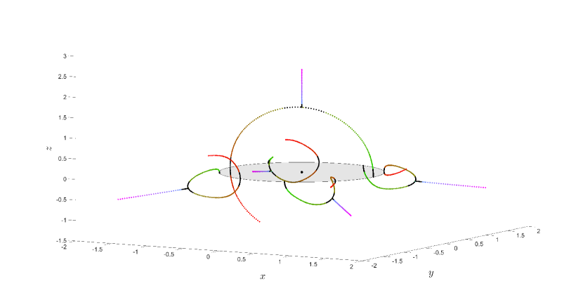
(a) $n=5$, $k=2$

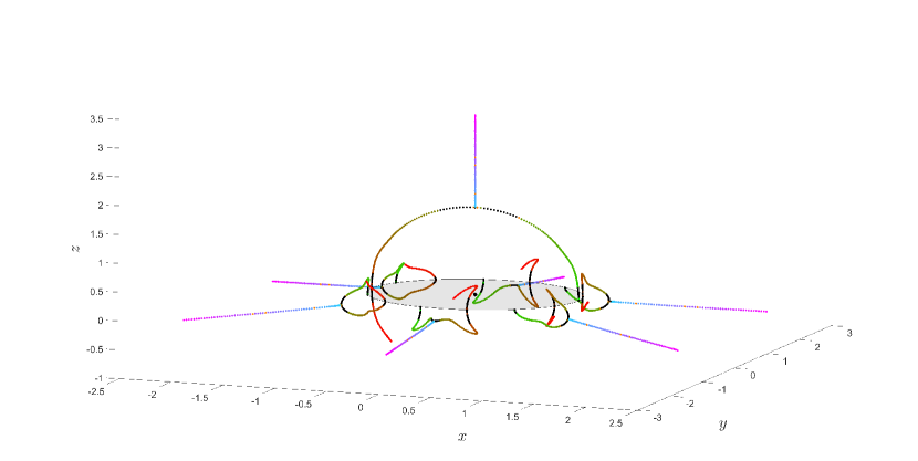
(b) $n=7$, $k=2$

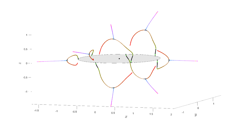
(c) $n=7$, $k=3$

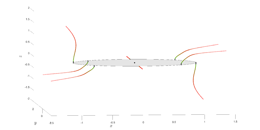
(d) $n=8$, $k=3$

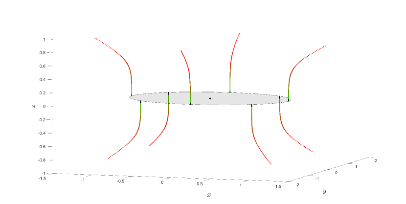
(e) $n=8$, $k=4$

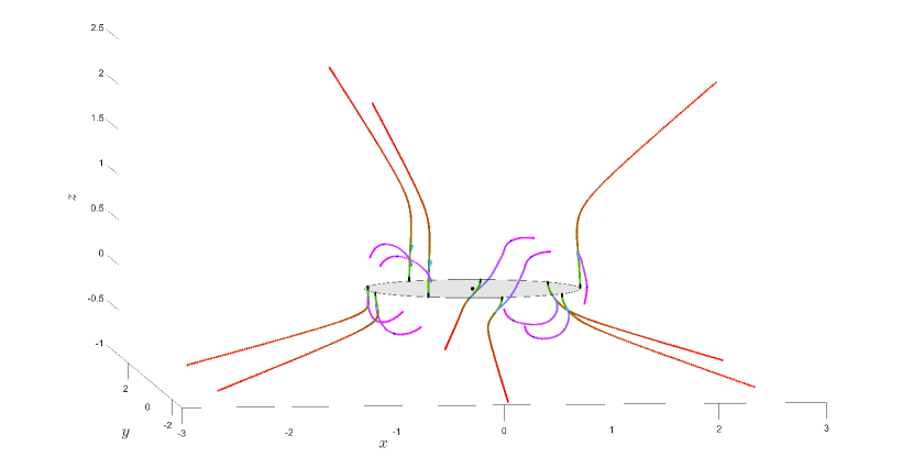
(f) $n=9$, $k=3$

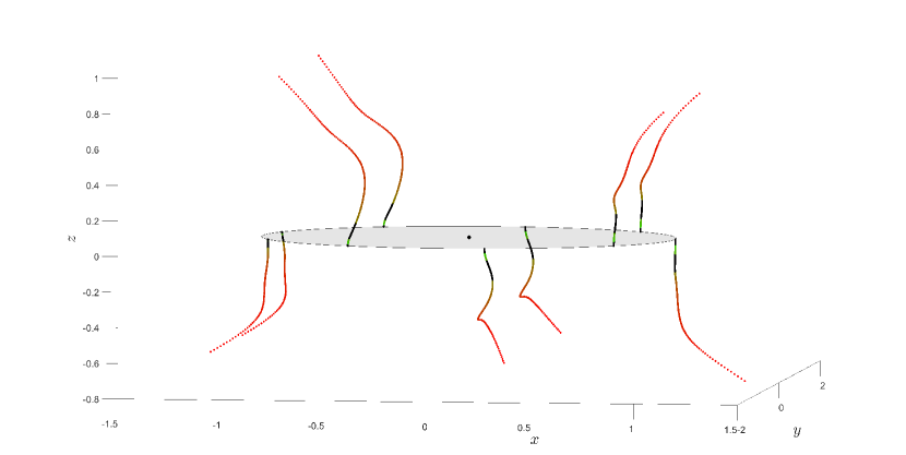
(g) $n=9$, $k=4$

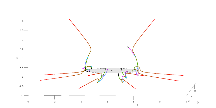
(h) $n=10$, $k=2$

Figure 3: Continuation of equilibria in the family $\mathfrak{F}_{1}^{k}$ for different values of $n$ and $k$. The colour coding in the figure is presented in Remark 3.2

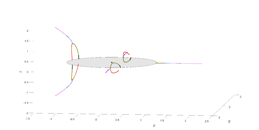
(a) $n=5$, $k=2$

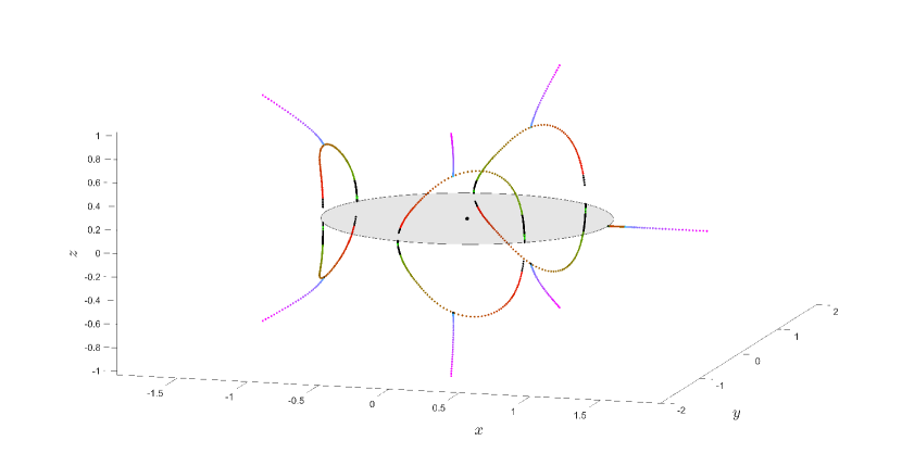
(b) $n=7$, $k=2$

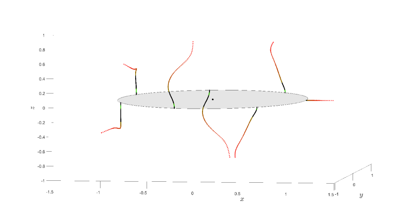
(c) $n=7$, $k=3$

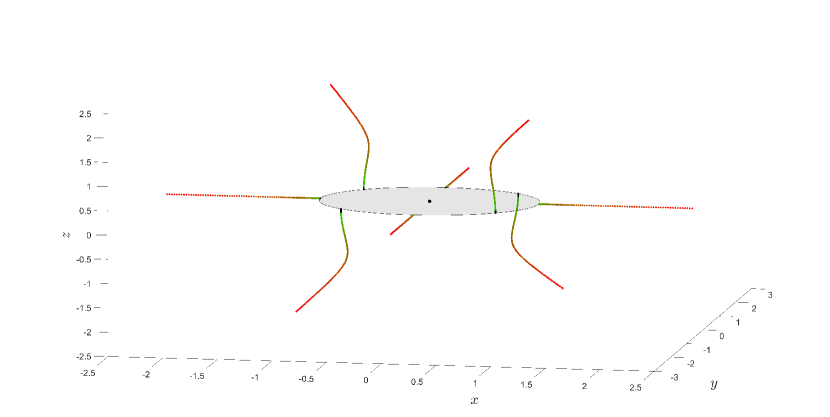
(d) $n=8$, $k=2$

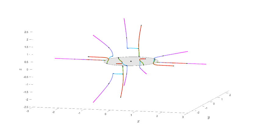
(e) $n=8$, $k=3$

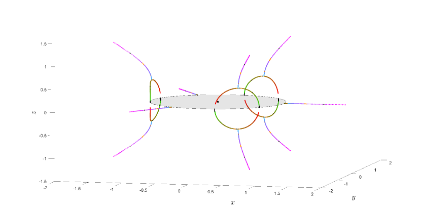
(f) $n=9$, $k=3$

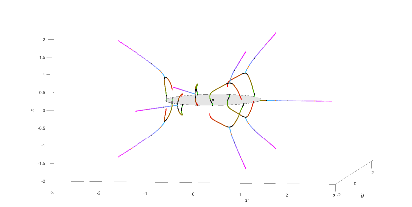
(g) $n=9$, $k=4$

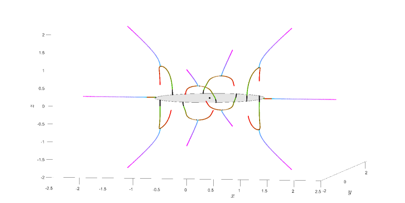
(h) $n=10$, $k=2$

Figure 4: Continuation of equilibria in the family $\mathfrak{F}_{2}^{k}$ for different values of $n$ and $k$. The colour coding in the figure is presented in Remark 3.2.

3.2 A computer-assisted validation of the spectra

The existence of non-trivial $2\pi/\nu$-periodic solutions of (3) arising from a spatial relative equilibrium $(u_{0};\mu_{0})$ relies on the validation of the hypotheses of Theorem 2.5; namely, to verify the existence of a $SO(2)$-nonresonant eigenvalue of $L(u_{0};\mu_{0})$ (see Definition 2.4). Now we turn our attention to prove this hypothesis by means of Theorem 3.1. Recall from Remark 2.3 that $\bar{\lambda},-\lambda,-\bar{\lambda}$ are eigenvalues of $L(u_{0};\mu_{0})$ if $\lambda\in\mathbb{C}$ is an eigenvalue of $L(u_{0};\mu_{0})$. Thus, if we prove the existence of a unique eigenvalue $\lambda_{0}$ in a neighbourhood $B_{\varepsilon}(i\bar{\nu})\subset\mathbb{C}$, then $\lambda_{0}=i\nu_{0}$ for some $\nu_{0}\in\mathbb{R}$ (i.e. $\lambda_{0}$ must be purely imaginary).

Recall that the existence of the relative equilibria $u_{0}\in B_{r_{0}}(\bar{u}_{0})$ is known via a successful application of Theorem 3.1, where $\bar{u}_{0}$ is a numerical solution and $r_{0}>0$ is the rigorous error bound. The validation of the eigenvalues of $L(u_{0};\mu_{0})$, which follows the approach [3], begins by finding numerically the eigenvalues of $L(\bar{u}_{0};\mu_{0})$. Denote by $\bar{\lambda}_{1},\dots,\bar{\lambda}_{6n}$ the numerical eigenvalues of $L(\bar{u}_{0};\mu_{0})$ (computed using the function eig.m in MATLAB, which returned the eigenvalues and their corresponding eigenvectors $\bar{v}_{1},\dots,\bar{v}_{6n}$). Fix $j\in\{1,\dots,6n\}$. Then, in order to obtain local isolation of the eigenpairs $(\lambda_{j},v_{j})\in\mathbb{C}\times\mathbb{C}^{6n}$, we rescale the eigenvector $v_{j}$ as follows. Denote by $k=k(j)$ the component of $\bar{v}_{j}$ with the largest magnitude, that is

$$|(\bar{v}_{j})_{k}|=\max_{\ell=1,\dots,6n}\left\{|(\bar{v}_{j})_{\ell}|\right\}.$$

Note that $k$ may not be unique. Then, the phase condition imposed to isolate the eigenpair $(\lambda_{j},v_{j})$ is $(v_{j})_{k}=(\bar{v}_{j})_{k}$, where recall that $\bar{v}_{j}\in\mathbb{C}^{6n}$ is the numerical approximation for $v_{j}$. The corresponding zero finding problem is setup in the following way

$$F_{\rm eig}(v,\lambda)\,\stackrel{{\scriptstyle\mbox{\tiny{\raisebox{0.0pt}[0.0pt][0.0pt]{def}}}}}{{=}}\,\begin{pmatrix}L(u_{0};\mu_{0})v-\lambda v\\ v\cdot e_{k}-(\bar{v}_{j})_{k}\end{pmatrix}=0,$$ (13)

where $\lambda$ and $v$ are the eigenvalue and eigenvector, respectively, and $e_{k}$ is the $k^{th}$ vector of the canonical basis of $\mathbb{R}^{6n}$. Without loss of generality, denote by $\lambda_{1}=\lambda_{2}=0$ the two zero eigenvalues of $L(u_{0};\mu_{0})$ due to the action of the group $SO(2)$. For each $j\in\{3,\dots,6n\}$, the rigorous enclosure of the eigenpair $(\lambda_{j},v_{j})$ is obtained by validated the existence of a solution of $F_{\rm eig}=0$ (where the map is defined in (13)) using Theorem 3.1. Denote by $r_{j}>0$ the radius of the ball $B_{r_{j}}(\bar{\lambda}_{j},\bar{v}_{j})\subset\mathbb{C}\times\mathbb{C}^{6n}$ which contains the unique eigenpair with $v\cdot e_{k}=(\bar{v}_{j})_{k}$, which we denote simply by $(\lambda_{j},v_{j})$.

For $j=3,\dots,6n$, denote by

$$D_{j}\,\stackrel{{\scriptstyle\mbox{\tiny{\raisebox{0.0pt}[0.0pt][0.0pt]{def}}}}}{{=}}\,\left\{z\in\mathbb{C}:|z_{j}-\bar{\lambda}_{j}|\leq r_{j}\right\}\subset\mathbb{C}$$

the disk which contains the true eigenvalue $\lambda_{j}$. Assume that numerically, two eigenvalues are given by $\pm i\bar{\nu}_{0}$, for some $\bar{\nu}_{0}>0$. Without loss of generality, denote by $\lambda_{3}$ and $\lambda_{4}$ the true eigenvalues such that

$$|\lambda_{3}-i\bar{\nu}_{0}|\leq r_{3}\quad\text{and}\quad|\lambda_{4}+i\bar{\nu}_{0}|\leq r_{4}.$$

By unicity, the true eigenvalues satisfy $\lambda_{3}=i\nu_{0}$ and $\lambda_{4}=-i\nu_{0}$, for some $\nu_{0}>0$ since otherwise the disk $D_{3}$ and $D_{4}$ would contain more eigenpairs by the comment above (see also Remark 2.3). Hence $\lambda_{3}=i\nu_{0}\in D_{3}$ and $\lambda_{4}=i\nu_{0}\in D_{4}$. Denote

$$\mathcal{D}\,\stackrel{{\scriptstyle\mbox{\tiny{\raisebox{0.0pt}[0.0pt][0.0pt]{def}}}}}{{=}}\,\bigcup_{j=5}^{6n}D_{j}$$

which contains rigorously $\lambda_{5},\dots,\lambda_{6n}$. The other four eigenvalues are given by $0,0,\pm i\nu_{0}$. For each spatial relative equilibria rigorously proven in Section 3.1, we verified rigorously that $\mathcal{D}\cap i\nu_{0}\tilde{\mathbb{N}}=\emptyset$ (where $\tilde{\mathbb{N}}\,\stackrel{{\scriptstyle\mbox{\tiny{\raisebox{0.0pt}[0.0pt][0.0pt]{def}}}}}{{=}}\,\{\ell\in\mathbb{Z}:\ell\geq 2\}$), hence showing rigorously that the eigenvalue $i\nu_{0}$ is a $SO(2)$-nonresonant eigenvalue. All of the computations were carried out in MATLAB using the library INTLAB [20].

Acknowledgements. JP.L. was partially supported by NSERC Discovery Grant. K.C. was partially supported by an ISM-CRM Undergraduate Summer Scholarship. C.G.A was partially supported by UNAM-PAPIIT project IA100121.

References

- [1] Felipe Alfaro Aguilar and Ernesto Pérez-Chavela. Relative equilibria in the charged n-body problem. The Canadian Applied Mathematics Quarterly, 10, 01 2002.
- [2] István Balázs, Jan Bouwe van den Berg, Julien Courtois, János Dudás, Jean-Philippe Lessard, Anett Vörös-Kiss, J. F. Williams, and Xi Yuan Yin. Computer-assisted proofs for radially symmetric solutions of PDEs. J. Comput. Dyn., 5(1-2):61–80, 2018.
- [3] Roberto Castelli and Jean-Philippe Lessard. A method to rigorously enclose eigenpairs of complex interval matrices. In Applications of mathematics 2013, pages 21–31. Acad. Sci. Czech Repub. Inst. Math., Prague, 2013.
- [4] Ian Davies, Aubrey Truman, and David Williams. Classical periodic solution of the equal-mass -body problem, -ion problem and the -electron atom problem. Phys. Lett. A, 99(1):15–18, 1983.
- [5] Sarah Day, Jean-Philippe Lessard, and Konstantin Mischaikow. Validated continuation for equilibria of PDEs. SIAM J. Numer. Anal., 45(4):1398–1424 (electronic), 2007.
- [6] Marco Fenucci and Àngel Jorba. Braids with the symmetries of Platonic polyhedra in the Coulomb -body problem. Commun. Nonlinear Sci. Numer. Simul., 83:105105, 12, 2020.
- [7] C. García-Azpeitia and J. Ize. Global bifurcation of polygonal relative equilibria for masses, vortices and dNLS oscillators. J. Differential Equations, 251(11):3202–3227, 2011.
- [8] C. García-Azpeitia and J. Ize. Global bifurcation of planar and spatial periodic solutions from the polygonal relative equilibria for the -body problem. J. Differential Equations, 254(5):2033–2075, 2013.
- [9] Allan Hungria, Jean-Philippe Lessard, and J. D. Mireles James. Rigorous numerics for analytic solutions of differential equations: the radii polynomial approach. Math. Comp., 85(299):1427–1459, 2016.
- [10] Jorge Ize and Alfonso Vignoli. Equivariant degree theory, volume 8 of De Gruyter Series in Nonlinear Analysis and Applications. Walter de Gruyter & Co., Berlin, 2003.
- [11] H. B. Keller. Lectures on numerical methods in bifurcation problems, volume 79 of Tata Institute of Fundamental Research Lectures on Mathematics and Physics. Published for the Tata Institute of Fundamental Research, Bombay, 1987. With notes by A. K. Nandakumaran and Mythily Ramaswamy.
- [12] R. Krawczyk. Newton-Algorithmen zur Bestimmung von Nullstellen mit Fehlerschranken. Computing (Arch. Elektron. Rechnen), 4:187–201, 1969.
- [13] Tim LaFave. Correspondences between the classical electrostatic thomson problem and atomic electronic structure. Journal of Electrostatics, 71(6):1029 – 1035, 2013.
- [14] Kenneth R. Meyer and Glen R. Hall. Introduction to Hamiltonian dynamical systems and the -body problem, volume 90 of Applied Mathematical Sciences. Springer-Verlag, New York, 1992.
- [15] Richard Moeckel. On central configurations. Mathematische Zeitschrift, 205(1):499–517, sep 1990.
- [16] Richard Moeckel and Carles Simó. Bifurcation of spatial central configurations from planar ones. SIAM Journal on Mathematical Analysis, 26(4):978–998, jul 1995.
- [17] R. E. Moore. A test for existence of solutions to nonlinear systems. SIAM J. Numer. Anal., 14(4):611–615, 1977.
- [18] Ramon E. Moore. Interval analysis. Prentice-Hall Inc., Englewood Cliffs, N.J., 1966.
- [19] F. J. Muñoz Almaraz, E. Freire, J. Galán, E. Doedel, and A. Vanderbauwhede. Continuation of periodic orbits in conservative and Hamiltonian systems. Phys. D, 181(1-2):1–38, 2003.
- [20] S.M. Rump. INTLAB - INTerval LABoratory. In Tibor Csendes, editor, Developments in Reliable Computing, pages 77–104. Kluwer Academic Publishers, Dordrecht, 1999. http://www.ti3.tu-harburg.de/rump/.