A short-memory operator splitting scheme for constant-Q viscoelastic wave equation

Yunfeng Xiong xiongyf@math.pku.edu.cn Xu Guo11footnotemark: 1 guoxu@sdu.edu.cn
Abstract

We propose a short-memory operator splitting scheme for solving the constant-Q wave equation, where the fractional stress-strain relation contains multiple Caputo fractional derivatives with order much smaller than 1. The key is to exploit its extension problem by converting the flat singular kernels into strongly localized ones, so that the major contribution of weakly singular integrals over a semi-infinite interval can be captured by a few Laguerre functions with proper asymptotic behavior. Despite its success in reducing both memory requirement and arithmetic complexity, we show that numerical accuracy under prescribed memory variables may deteriorate in time due to the dynamical increments of projection errors. Fortunately, it can be considerably alleviated by introducing a suitable scaling factor β>1𝛽1\beta>1 and pushing the collocation points closer to origin. An operator splitting scheme is introduced to solve the resulting set of equations, where the auxiliary dynamics can be solved exactly, so that it gets rid of the numerical stiffness and discretization errors. Numerical experiments on both 1-D diffusive wave equation and 2-D constant-Q P𝑃P- and S𝑆S-wave equations are presented to validate the accuracy and efficiency of the proposed scheme.

keywords:
Viscoelastic wave equation , Caputo fractional derivative , Laguerre spectral method , Scaling technique , Short-memory principle
MSC:
[2010] , 65M22 , 74S25 , 41A05 , 35R11 , 33F05
\affiliation

[label1]organization=LMAM and School of Mathematical Sciences, Peking University,postcode=100871, state=Beijing, country=China

\affiliation

[label2]organization=Geotechnical and Structural Research Center, Shandong University,city=Jinan, postcode=250061, state=Shandong, country=China

1 Introduction

Seismic wave propagation has anelastic characteristics in real earth materials due to the loss of energy by the geometrical effect of the enlargement of the wavefront and by the intrinsic absorption of the earth [1, 2, 3]. Thus both the effects of attenuation and velocity dispersion should be taken into account for obtaining an accurate wavefield modeling. Among various models, Kjartansson’s constant-Q model containing the fractional strain-stress relation provides a concise description of the wave attenuation by only two parameters: Q𝑄Q for the portion of energy lost and c0subscript𝑐0c_{0} for the phase velocity [1, 4], and the quality factor Q𝑄Q is usually observed as a frequency-independent (constant) parameter [5, 6]. In most circumstances the loss caused by scattering and absorption is relatively small, so that the attenuation of the seismic energy is treated as a small perturbation on the propagation [1, 5]. Following the basic idea of Kjartansson’s model, Carcione developed the theory of constant-Q P𝑃P- and S𝑆S- wave modeling and derived a set of parabolic equations involving multiple temporal Caputo fractional derivatives, which exhibit different attenuation levels in different propagation directions [7]. In the past few decades, 2-D and 3-D constant-Q wave modelings, as well as their variants, have been drawing a growing attention in various seismic applications [8, 9, 10, 11].

Despite its mathematical elegance, solving the constant-Q wave equation remains a huge numerical challenge due to the extremely high memory requirement and high arithmetic complexity induced by the very small fractional power [12], which is about 103superscript10310^{-3} to 101superscript10110^{-1} in real viscoelastic media [3]. In recent years, many sophisticated algorithms have been proposed to tackle the Caputo fractional derivatives in the diffusive wave models, such as the finite difference schemes based on the weighted Grünwald-Letnikov formula [7, 13] and those based on the interpolation polynomials [14, 15], the spectral collocation method [16] and the meshless method [17], but their efficiency might still be hampered by the storage of long history. It has been reported by the author of [18] that the storage of 500500500 memory length and the grid of 1203superscript1203120^{3} in a 3-D orthorhombic example requires approximately 909090GB computer memory, thereby dramatically restricting the numerical resolution and hampering its usage in real seismic applications such as reverse time migration. For this reason, the authors of [19, 8, 20] suggested to replace the temporal fractional derivative by a spatial fractional Laplacian operator with the same dispersion relation and developed efficient numerical algorithms for the resulting memory-free nonlocal wave equations [21, 8, 22, 11]. However, it still requires to establish their rigorous mathematical connection, especially when the artificial boundary conditions are involved [23].

Intuitively speaking, the drawback of long-memory requirement in the existing algorithms is rooted in the flatness of the singular kernel in the Caputo fractional derivative, so that the remedy is to seek a localization of such kernel. Our short-memory operator splitting (SMOS) scheme is based on the extension problem of the Caputo derivative by introducing an extra memory variable y(0,+)𝑦0y\in(0,+\infty) [24, 25], and the initial effective condition must be derived from the fractional strain-stress relation to preserve the proper asymptotic behavior. In this way, the original constant-Q wave equation can be reformulated into an equivalent set of dynamical system without fractional derivatives, but involving an integral over a semi-infinite domain with a strongly localized Abel kernel. Such nonlocal component is usually resolved by the Laguerre-Gauss quadrature in the spirit of the Yuan-Agrawal method [26, 27] or the diffusive approximation [28, 12]. Compared with the sum-of-exponentials technique [15], the Yuan-Agrawal method allows a simpler truncation as the major contribution of the pre-asymptotic range of the weakly singular integral can be accurately captured by only a few Laguerre-Gauss quadrature nodes (memory variables) [12, 29].

Regarding that the Yuan-Agrawal method still lacks a rigorous theoretical justification, we provide a thorough analysis of the dynamical errors within the framework of generalized Laguerre interpolation [30, 31, 32, 33, 34] and point out its potential weakness, that is, the dynamical increments of projection errors due to the impulse (non-decay) of the source term. In other words, the numerical accuracy under the prescribed number of collocation points may deteriorate sharply in time evolution. Fortunately, we also show that it can be significantly alleviated by introducing a scaling factor β>1𝛽1\beta>1 in the Laguerre functions and pushing the collocations points closer to origin. Another challenge is the severe numerical stiffness in solving the auxiliary dynamics, which usually requires the usage of A𝐴A-stable implicit integrators and introduces additional numerical errors [12]. SMOS utilizes a key observation that although it breaks the Hamiltonian structure of the elastic counterpart, the constant-Q wave equation can still be evolved by an appropriate operator splitting. In particular, the auxiliary equations can be solved exactly, thereby getting rid of the numerical stiffness and significantly boosting the numerical stability. Numerical experiments also validate that the Strang splitting can achieve a second-order convergence in time, and higher-order scheme can be achieved in principle by Yoshida’s method [35]. Combining these ingredients together allows us to maintain the accuracy, to significantly shorten the effective memory length and to reduce the arithmetic complexity simultaneously.

The rest of this paper is organized as follows. In Section 2 we briefly review the constant-Q viscoelastic wave equation and derive its extension problem, as well as the proper initial condition. In Section 3, we will first analyze the dynamical increments of Laguerre-Gauss projection errors and present how the scaling factor β>1𝛽1\beta>1 enhances the accuracy, then give the operator splitting scheme. Numerical experiments on both 1-D diffusive wave equation and 2-D constant-Q wave equation are presented in Section 4 to validate the convergence, accuracy and efficiency of the proposed scheme. Specifically, the relation between the number of memory variables and accuracy will be carefully investigated. The conclusion and several discussions are drawn in Section 5.

2 The extension problem of constant-Q wave equation

The dynamics of constant-Q wave propagation are governed by three sets of equations with 𝒙d𝒙superscript𝑑\bm{x}\in\mathbb{R}^{d}, d3𝑑3d\leq 3 [7]. The first set is the conservation of linear momentum:

ρ(𝒙)2t2ui(𝒙,t)=xjσij(𝒙,t)+fi(𝒙,t),i,j=1,,3,formulae-sequence𝜌𝒙superscript2superscript𝑡2subscript𝑢𝑖𝒙𝑡subscript𝑥𝑗subscript𝜎𝑖𝑗𝒙𝑡subscript𝑓𝑖𝒙𝑡𝑖𝑗13\rho(\bm{x})\frac{\partial^{2}}{\partial t^{2}}u_{i}(\bm{x},t)=\frac{\partial}{\partial x_{j}}\sigma_{ij}(\bm{x},t)+f_{i}(\bm{x},t),\quad i,j=1,\dots,3, (2.1)

where σijsubscript𝜎𝑖𝑗\sigma_{ij} are the components of the stress tensor, uisubscript𝑢𝑖u_{i} are the components of the displacement vector, ρ𝜌\rho is the mass density and fisubscript𝑓𝑖f_{i} are components of the body forces per unit (source term). The summation over repeated indices j𝑗j is assumed in Eq. (2.1). The second set is the definition of strain tensor εijsubscript𝜀𝑖𝑗\varepsilon_{ij}, which can be obtained in terms of the displacement components as

εij(𝒙,t)=12(xiuj(𝒙,t)+xjui(𝒙,t)),i,j=1,,3.formulae-sequencesubscript𝜀𝑖𝑗𝒙𝑡12subscript𝑥𝑖subscript𝑢𝑗𝒙𝑡subscript𝑥𝑗subscript𝑢𝑖𝒙𝑡𝑖𝑗13\varepsilon_{ij}(\bm{x},t)=\frac{1}{2}\left(\frac{\partial}{\partial x_{i}}u_{j}(\bm{x},t)+\frac{\partial}{\partial x_{j}}u_{i}(\bm{x},t)\right),\quad i,j=1,\dots,3. (2.2)

The constitutive equation, or the stress-strain relation, involves a relaxation by power creep functions. Equivalently, it contains temporal Caputo fractional derivatives [4, 7],

σij=MP(𝒙)Γ(12γP)(tt0)2γPH(t)tεij2MS(𝒙)Γ(12γS)(tt0)2γSH(t)tεij=(𝒙)Dt2γPCεkkδij+2μ(𝒙)Dt2γSC[εijεkkδij],subscript𝜎𝑖𝑗subscript𝑀𝑃𝒙Γ12subscript𝛾𝑃superscript𝑡subscript𝑡02subscript𝛾𝑃𝐻𝑡𝑡subscript𝜀𝑖𝑗2subscript𝑀𝑆𝒙Γ12subscript𝛾𝑆superscript𝑡subscript𝑡02subscript𝛾𝑆𝐻𝑡𝑡subscript𝜀𝑖𝑗𝒙subscriptsuperscriptsubscript𝐷𝑡2subscript𝛾𝑃𝐶subscript𝜀𝑘𝑘subscript𝛿𝑖𝑗2𝜇𝒙subscriptsuperscriptsubscript𝐷𝑡2subscript𝛾𝑆𝐶delimited-[]subscript𝜀𝑖𝑗subscript𝜀𝑘𝑘subscript𝛿𝑖𝑗\begin{split}\sigma_{ij}=&\frac{M_{P}(\bm{x})}{\Gamma(1-2\gamma_{P})}\left(\frac{t}{t_{0}}\right)^{-2\gamma_{P}}H(t)\ast\frac{\partial}{\partial t}\varepsilon_{ij}-\frac{2M_{S}(\bm{x})}{\Gamma(1-2\gamma_{S})}\left(\frac{t}{t_{0}}\right)^{-2\gamma_{S}}H(t)\ast\frac{\partial}{\partial t}\varepsilon_{ij}\\ =&\mathcal{E}(\bm{x}){{}_{C}}D_{t}^{2\gamma_{P}}\varepsilon_{kk}\delta_{ij}+2\mu(\bm{x}){{}_{C}}D_{t}^{2\gamma_{S}}\left[\varepsilon_{ij}-\varepsilon_{kk}\delta_{ij}\right],\end{split} (2.3)

where the definition of the extended Caputo fractional derivative reads that

DtαC𝜺{1Γ(1α)0t(tτ)α[τ𝜺(𝒙,τ)]dτ,0<α<1,1Γ(2α)0t(tτ)1α[2τ2𝜺(𝒙,τ)]dτ,1<α<2,{{}_{C}}D_{t}^{\alpha}\bm{\varepsilon}\coloneqq\left\{\begin{split}&\frac{1}{\Gamma(1-\alpha)}\int_{0}^{t}(t-\tau)^{-\alpha}\left[\frac{\partial}{\partial\tau}\bm{\varepsilon}(\bm{x},\tau)\right]\textup{d}\tau,&\quad 0<\alpha<1,\\ &\frac{1}{\Gamma(2-\alpha)}\int_{0}^{t}(t-\tau)^{1-\alpha}\left[\frac{\partial^{2}}{\partial\tau^{2}}\bm{\varepsilon}(\bm{x},\tau)\right]\textup{d}\tau,&\quad 1<\alpha<2,\end{split}\right. (2.4)

and MP(𝒙)=ρ(𝒙)cP2cos2(πγP2),MS(𝒙)=ρ(𝒙)cS2cos2(πγS2)formulae-sequencesubscript𝑀𝑃𝒙𝜌𝒙superscriptsubscript𝑐𝑃2superscript2𝜋subscript𝛾𝑃2subscript𝑀𝑆𝒙𝜌𝒙superscriptsubscript𝑐𝑆2superscript2𝜋subscript𝛾𝑆2M_{P}(\bm{x})=\rho(\bm{x})c_{P}^{2}\cos^{2}\left(\frac{\pi\gamma_{P}}{2}\right),M_{S}(\bm{x})=\rho(\bm{x})c_{S}^{2}\cos^{2}\left(\frac{\pi\gamma_{S}}{2}\right) are bulk moduli, cPsubscript𝑐𝑃c_{P} and cSsubscript𝑐𝑆c_{S} are P𝑃P-wave and S𝑆S-wave velocities, respectively, ΓΓ\Gamma is the Euler’s Gamma function, t0subscript𝑡0t_{0} is the same reference time, γP,γSsubscript𝛾𝑃subscript𝛾𝑆\gamma_{P},\gamma_{S} are dimensionless parameters, and H𝐻H is the Heaviside step function. The summation over repeated indices k𝑘k is assumed in Eq. (2.3). The powers γP,γSsubscript𝛾𝑃subscript𝛾𝑆\gamma_{P},\gamma_{S} of the fractional derivatives are characterized by constant quality factors QPsubscript𝑄𝑃Q_{P} and QSsubscript𝑄𝑆Q_{S} for P𝑃P- and S𝑆S- waves, respectively.

γP=π1tan1(QP1),γS=π1tan1(QS1).formulae-sequencesubscript𝛾𝑃superscript𝜋1superscript1superscriptsubscript𝑄𝑃1subscript𝛾𝑆superscript𝜋1superscript1superscriptsubscript𝑄𝑆1\gamma_{P}=\pi^{-1}\tan^{-1}(Q_{P}^{-1}),\quad\gamma_{S}=\pi^{-1}\tan^{-1}(Q_{S}^{-1}). (2.5)

The main difficulty in solving the constant-Q wave equation lies in the singular kernel (tτ)2γsuperscript𝑡𝜏2𝛾(t-\tau)^{-2\gamma} in Eq. (2.4) since it is global and rather flat when γ1much-less-than𝛾1\gamma\ll 1, so that direct discretization requires to store a long history to maintain the accuracy. A localization of the singular kernel can be achieved by introducing an auxiliary function Φ[𝜺](𝒙,y,t)Φdelimited-[]𝜺𝒙𝑦𝑡\Phi[\bm{\varepsilon}](\bm{x},y,t) with an extra memory variable y𝑦y, so that it extends the constant-Q wave equation into another nonlocal problem with an extra dimension. Such essential idea was exploited in the Yuan-Agrawal method [26, 27] and the diffusive approximation [28].

In the following part, we will derive the extension problem of the Caputo fractional derivative. As typical examples, the extension of unidimensional and two-dimensional constant-Q wave equations are provided. Then we try to give an initial condition for the auxiliary functions Φ[𝜺](𝒙,y,t)Φdelimited-[]𝜺𝒙𝑦𝑡\Phi[\bm{\varepsilon}](\bm{x},y,t), which was usually assumed to be zero in the previous literatures [26, 27, 12]. But actually it must be derived from the stress-strain relation as the violation may lead to incorrect asymptotic behavior [36].

2.1 Extension problem

The extension of the fractional derivative (2.4) is known as the fractional power in functional analysis [24, 26], which is also the basis of the Yuan-Agrawal method,

DtαC𝜺(𝒙,t)=1Γ(1α)0t(tτ)α[τ𝜺(𝒙,τ)]dτ=sin(πα)π0+0t𝕖zzα1(tτ)α[τ𝜺(𝒙,τ)]dτdz=2sin(πα)π0+0ty2α1𝕖(tτ)y2[τ𝜺(𝒙,τ)]dτdy,subscriptsuperscriptsubscript𝐷𝑡𝛼𝐶𝜺𝒙𝑡1Γ1𝛼superscriptsubscript0𝑡superscript𝑡𝜏𝛼delimited-[]𝜏𝜺𝒙𝜏d𝜏𝜋𝛼𝜋superscriptsubscript0superscriptsubscript0𝑡superscript𝕖𝑧superscript𝑧𝛼1superscript𝑡𝜏𝛼delimited-[]𝜏𝜺𝒙𝜏d𝜏d𝑧2𝜋𝛼𝜋superscriptsubscript0superscriptsubscript0𝑡superscript𝑦2𝛼1superscript𝕖𝑡𝜏superscript𝑦2delimited-[]𝜏𝜺𝒙𝜏d𝜏d𝑦\begin{split}{{}_{C}}D_{t}^{\alpha}\bm{\varepsilon}(\bm{x},t)&=\frac{1}{\Gamma(1-\alpha)}\int_{0}^{t}(t-\tau)^{-\alpha}\left[\frac{\partial}{\partial\tau}\bm{\varepsilon}(\bm{x},\tau)\right]\textup{d}\tau\\ &=\frac{\sin(\pi\alpha)}{\pi}\int_{0}^{+\infty}\int_{0}^{t}\frac{\mathbbm{e}^{-z}z^{\alpha-1}}{(t-\tau)^{\alpha}}\left[\frac{\partial}{\partial\tau}\bm{\varepsilon}(\bm{x},\tau)\right]\textup{d}\tau\textup{d}z\\ &=\frac{2\sin(\pi\alpha)}{\pi}\int_{0}^{+\infty}\int_{0}^{t}y^{2\alpha-1}\mathbbm{e}^{-(t-\tau)y^{2}}\left[\frac{\partial}{\partial\tau}\bm{\varepsilon}(\bm{x},\tau)\right]\textup{d}\tau\textup{d}y,\end{split} (2.6)

where the second equality utilizes the reflection formula for the Gamma function,

Γ(α)=0+𝕖zzα1dz,Γ(α)Γ(1α)=πsin(πα).formulae-sequenceΓ𝛼superscriptsubscript0superscript𝕖𝑧superscript𝑧𝛼1d𝑧Γ𝛼Γ1𝛼𝜋𝜋𝛼\Gamma(\alpha)=\int_{0}^{+\infty}\mathbbm{e}^{-z}z^{\alpha-1}\textup{d}z,\quad\Gamma(\alpha)\Gamma(1-\alpha)=\frac{\pi}{\sin(\pi\alpha)}. (2.7)

The third equality can be verified by the variable substitution z=(tτ)y2𝑧𝑡𝜏superscript𝑦2z=(t-\tau)y^{2}.

Now we define the auxiliary function Φ[𝜺](𝒙,y,t):d××[0,):Φdelimited-[]𝜺𝒙𝑦𝑡superscript𝑑0\Phi[\bm{\varepsilon}](\bm{x},y,t):\mathbb{R}^{d}\times\mathbb{R}\times[0,\infty)\to\mathbb{R} with an extra variable,

Φ[𝜺](𝒙,y,t)=0t𝕖(tτ)y2[τ𝜺(𝒙,τ)]dτ.Φdelimited-[]𝜺𝒙𝑦𝑡superscriptsubscript0𝑡superscript𝕖𝑡𝜏superscript𝑦2delimited-[]𝜏𝜺𝒙𝜏d𝜏\Phi[\bm{\varepsilon}](\bm{x},y,t)=\int_{0}^{t}\mathbbm{e}^{-(t-\tau)y^{2}}\left[\frac{\partial}{\partial\tau}\bm{\varepsilon}(\bm{x},\tau)\right]\textup{d}\tau. (2.8)

It deserves to mention that our definition of Φ[𝜺](𝒙,y,t)Φdelimited-[]𝜺𝒙𝑦𝑡\Phi[\bm{\varepsilon}](\bm{x},y,t) is slightly different from that in [26], where the singular kernel is incorporated into the auxiliary function. This gets rid of the singularity at y0+𝑦superscript0y\to 0^{+} in the definition, as well as the dependence on the fractional order γ𝛾\gamma.

According to Eq. (2.8), it satisfies the auxiliary relaxed dynamics,

tΦ[𝜺](𝒙,y,t)=t𝜺(𝒙,t)y2Φ[𝜺](𝒙,y,t),𝑡Φdelimited-[]𝜺𝒙𝑦𝑡𝑡𝜺𝒙𝑡superscript𝑦2Φdelimited-[]𝜺𝒙𝑦𝑡\frac{\partial}{\partial t}\Phi[\bm{\varepsilon}](\bm{x},y,t)=\frac{\partial}{\partial t}\bm{\varepsilon}(\bm{x},t)-y^{2}\Phi[\bm{\varepsilon}](\bm{x},y,t), (2.9)

and the fractional Caputo derivative is represented as a weakly singular integral

DtαC𝜺(𝒙,t)=2sin(πα)π0+y2α1Φ[𝜺](𝒙,y,t)dy.subscriptsuperscriptsubscript𝐷𝑡𝛼𝐶𝜺𝒙𝑡2𝜋𝛼𝜋superscriptsubscript0superscript𝑦2𝛼1Φdelimited-[]𝜺𝒙𝑦𝑡d𝑦{{}_{C}}D_{t}^{\alpha}\bm{\varepsilon}(\bm{x},t)=\frac{2\sin(\pi\alpha)}{\pi}\int_{0}^{+\infty}y^{2\alpha-1}\Phi[\bm{\varepsilon}](\bm{x},y,t)\textup{d}y. (2.10)

Let g(𝒙,t)=tε(𝒙,t)𝑔𝒙𝑡𝑡𝜀𝒙𝑡g(\bm{x},t)=\frac{\partial}{\partial t}\varepsilon(\bm{x},t), then the exact solution of the auxiliary dynamics (2.9) reads that

Φ[𝜺](𝒙,y,t)=𝕖y2tΦ[𝜺](𝒙,y,0)+0t𝕖y2τg(𝒙,tτ)dτ.Φdelimited-[]𝜺𝒙𝑦𝑡superscript𝕖superscript𝑦2𝑡Φdelimited-[]𝜺𝒙𝑦0superscriptsubscript0𝑡superscript𝕖superscript𝑦2𝜏𝑔𝒙𝑡𝜏d𝜏\Phi[\bm{\varepsilon}](\bm{x},y,t)=\mathbbm{e}^{-y^{2}t}\Phi[\bm{\varepsilon}](\bm{x},y,0)+\int_{0}^{t}\mathbbm{e}^{-y^{2}\tau}g(\bm{x},t-\tau)\textup{d}\tau. (2.11)

For sufficiently large y𝑦y and by integrations by parts, it has that

Φ[ε](𝒙,y,t)=𝕖y2tϕ(y,0)+1y2[g(𝒙,t)𝕖y2tg(𝒙,0)]+0t𝕖y2τtg(𝒙,tτ)dτ,Φdelimited-[]𝜀𝒙𝑦𝑡superscript𝕖superscript𝑦2𝑡italic-ϕ𝑦01superscript𝑦2delimited-[]𝑔𝒙𝑡superscript𝕖superscript𝑦2𝑡𝑔𝒙0superscriptsubscript0𝑡superscript𝕖superscript𝑦2𝜏𝑡𝑔𝒙𝑡𝜏d𝜏\begin{split}\Phi[\varepsilon](\bm{x},y,t)=&\mathbbm{e}^{-y^{2}t}\phi(y,0)+\frac{1}{y^{2}}\left[g(\bm{x},t)-\mathbbm{e}^{-y^{2}t}g(\bm{x},0)\right]\\ &+\int_{0}^{t}\mathbbm{e}^{-y^{2}\tau}\frac{\partial}{\partial t}g(\bm{x},t-\tau)\textup{d}\tau,\end{split} (2.12)

which implies that Eq. (2.10) is well defined since Φ[𝜺]Φdelimited-[]𝜺\Phi[\bm{\varepsilon}] decays as 𝒪(y2)𝒪superscript𝑦2\mathcal{O}(y^{-2}).

By introducing the velocity vector 𝒗(𝒙,t)=t𝒖(𝒙,t)𝒗𝒙𝑡𝑡𝒖𝒙𝑡\bm{v}(\bm{x},t)=\frac{\partial}{\partial t}\bm{u}(\bm{x},t) to replace 𝒖𝒖\bm{u}, the extension problem of the constant-Q wave equation is cast into a parabolic system,

t(𝒗𝝈Φ[𝜺])=(03000210y2d)(𝒗𝝈Φ[𝜺])+(𝒇00).𝑡matrix𝒗𝝈Φdelimited-[]𝜺matrix0subscript3000subscript2subscript10superscript𝑦2subscript𝑑matrix𝒗𝝈Φdelimited-[]𝜺matrix𝒇00\frac{\partial}{\partial t}\begin{pmatrix}\bm{v}\\ \bm{\sigma}\\ \Phi[\bm{\varepsilon}]\end{pmatrix}=\begin{pmatrix}0&\mathcal{L}_{3}&0\\ 0&0&\mathcal{L}_{2}\\ \mathcal{L}_{1}&0&-y^{2}\mathcal{I}_{d}\end{pmatrix}\begin{pmatrix}\bm{v}\\ \bm{\sigma}\\ \Phi[\bm{\varepsilon}]\end{pmatrix}+\begin{pmatrix}\bm{f}\\ 0\\ 0\end{pmatrix}. (2.13)

or equivalently,

t(𝒗Φ[𝜺])=(0321y2d)(𝒗Φ[𝜺])+(𝒇0)𝑡matrix𝒗Φdelimited-[]𝜺matrix0subscript3subscript2subscript1superscript𝑦2subscript𝑑matrix𝒗Φdelimited-[]𝜺matrix𝒇0\frac{\partial}{\partial t}\begin{pmatrix}\bm{v}\\ \Phi[\bm{\varepsilon}]\end{pmatrix}=\begin{pmatrix}0&\mathcal{L}_{3}\circ\mathcal{L}_{2}\\ \mathcal{L}_{1}&-y^{2}\mathcal{I}_{d}\end{pmatrix}\begin{pmatrix}\bm{v}\\ \Phi[\bm{\varepsilon}]\end{pmatrix}+\begin{pmatrix}\bm{f}\\ 0\end{pmatrix} (2.14)

with dsubscript𝑑\mathcal{I}_{d} a d×d𝑑𝑑d\times d identity matrix. The operator y2dsuperscript𝑦2subscript𝑑y^{2}\mathcal{I}_{d} breaks the Hamiltonian structure of the elastic wave equation and results in a relaxation in Φ[𝜺]Φdelimited-[]𝜺\Phi[\bm{\varepsilon}].

2.2 Typical examples

Now we give two typical examples of constant-Q wave equation that characterizes an interpolated regime between the wave propagation and the heat diffusion. In unidimensional case, the stress-strain relation is that

σ(x,t)=Cρ(x)Dt2γCε(x,t),𝜎𝑥𝑡𝐶𝜌𝑥subscriptsuperscriptsubscript𝐷𝑡2𝛾𝐶𝜀𝑥𝑡\sigma(x,t)=C\rho(x){{}_{C}}D_{t}^{2\gamma}\varepsilon(x,t), (2.15)

where C𝐶C is a constant depending on c0,γ,t0subscript𝑐0𝛾subscript𝑡0c_{0},\gamma,t_{0}. For its extension, the linear bounded operator 2subscript2\mathcal{L}_{2} and the gradient operators 1subscript1\mathcal{L}_{1}, 3subscript3\mathcal{L}_{3} are given by

1v(x,t)subscript1𝑣𝑥𝑡\displaystyle\mathcal{L}_{1}v(x,t) =1ρ(x)xv(x,t),absent1𝜌𝑥𝑥𝑣𝑥𝑡\displaystyle=\frac{1}{\rho(x)}\frac{\partial}{\partial x}v(x,t), (2.16)
(2Φ[𝜺])(x,t)subscript2Φdelimited-[]𝜺𝑥𝑡\displaystyle(\mathcal{L}_{2}\Phi[\bm{\varepsilon}])(x,t) =2Csin(2πγ)π[ρ(x)0+y4γ1Φ[𝜺](x,y,t)dy],absent2𝐶2𝜋𝛾𝜋delimited-[]𝜌𝑥superscriptsubscript0superscript𝑦4𝛾1Φdelimited-[]𝜺𝑥𝑦𝑡d𝑦\displaystyle=\frac{2C\sin(2\pi\gamma)}{\pi}\left[\rho(x)\int_{0}^{+\infty}y^{4\gamma-1}\Phi[\bm{\varepsilon}](x,y,t)\textup{d}y\right], (2.17)
3σ(x,t)subscript3𝜎𝑥𝑡\displaystyle\mathcal{L}_{3}\sigma(x,t) =ρ(x)xσ(x,t).absent𝜌𝑥𝑥𝜎𝑥𝑡\displaystyle=\rho(x)\frac{\partial}{\partial x}\sigma(x,t). (2.18)

Equivalently, substituting (2.15) into Eqs. (2.1) and (2.2) yields that

2t2v(x,t)=Cρ(x)x(ρ(x)xDt2γCv(x,t))+tf(x,t).superscript2superscript𝑡2𝑣𝑥𝑡𝐶𝜌𝑥𝑥𝜌𝑥𝑥subscriptsuperscriptsubscript𝐷𝑡2𝛾𝐶𝑣𝑥𝑡𝑡𝑓𝑥𝑡\frac{\partial^{2}}{\partial t^{2}}v(x,t)=\frac{C}{\rho(x)}\frac{\partial}{\partial x}\left(\rho(x)\frac{\partial}{\partial x}{{}_{C}}D_{t}^{2\gamma}v(x,t)\right)+\frac{\partial}{\partial t}f(x,t). (2.19)

When ρ(x)=ρ0𝜌𝑥subscript𝜌0\rho(x)=\rho_{0} is constant and tf(x,t)0𝑡𝑓𝑥𝑡0\frac{\partial}{\partial t}f(x,t)\equiv 0, it reduces to the standard diffusive wave equation

Dt22γCv(x,t)=C2x2v(x,t).subscriptsuperscriptsubscript𝐷𝑡22𝛾𝐶𝑣𝑥𝑡𝐶superscript2superscript𝑥2𝑣𝑥𝑡{{}_{C}}D_{t}^{2-2\gamma}v(x,t)=C\frac{\partial^{2}}{\partial x^{2}}v(x,t). (2.20)

For v(x,0+)=v0(x)𝑣𝑥superscript0subscript𝑣0𝑥v(x,0^{+})=v_{0}(x) and tv(x,0+)=0𝑡𝑣𝑥superscript00\frac{\partial}{\partial t}v(x,0^{+})=0, the exact solution reads that

v(x,t)=+G(xy,t;1γ)v0(y)dy,𝑣𝑥𝑡superscriptsubscript𝐺𝑥𝑦𝑡1𝛾subscript𝑣0𝑦d𝑦\begin{split}v(x,t)=\int_{-\infty}^{+\infty}G(x-y,t;1-\gamma)v_{0}(y)\textup{d}y,\end{split} (2.21)

where the Green’s function G(x,t;ν)𝐺𝑥𝑡𝜈G(x,t;\nu) is given by

G(x,t;ν)=12CtνMν(xCtν),𝐺𝑥𝑡𝜈12𝐶superscript𝑡𝜈subscript𝑀𝜈𝑥𝐶superscript𝑡𝜈G(x,t;\nu)=\frac{1}{2\sqrt{C}t^{\nu}}M_{\nu}\left(\frac{x}{\sqrt{C}t^{\nu}}\right), (2.22)

and the Mainardi function Mν(x)subscript𝑀𝜈𝑥M_{\nu}(x) is a special kind of the Wright function of the second kind [4], namely, Mν(z)Wν,1ν(z),0<ν<1formulae-sequencesubscript𝑀𝜈𝑧subscript𝑊𝜈1𝜈𝑧0𝜈1M_{\nu}(z)\coloneqq W_{-\nu,1-\nu}(-z),0<\nu<1.

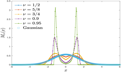
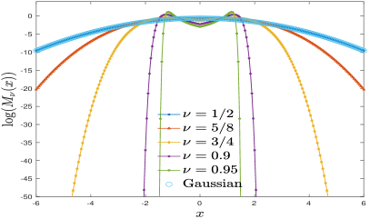
Intuitively, the temporal fractional PDE (2.20) describes the intermediate state of pure diffusion and pure wave dispersion, known as the fractional diffusion-wave phenomenon [4]. The Mainardi function under different ν𝜈\nu is presented in Figure 9. When γ=1/2𝛾12\gamma=1/2, it corresponds to the heat kernel and describes the wave dissipation. When γ=0𝛾0\gamma=0, it corresponds to the wave equation and describes the wave dispersion. For 0<γ<1/20𝛾120<\gamma<1/2, the solution may exhibit both wave dissipation and velocity dispersion.

Now considering the wave propagation in two-dimensional (x,z)𝑥𝑧(x,z)-domain, the stress-strain relation reads that [7, 8]

σ11(x,z,t)ρ(x,z)=CPDtγPC(ε11(x,z,t)+ε33(x,z,t))2CSDtγSCε33(x,z,t),σ33(x,z,t)ρ(x,z)=CPDtγPC(ε11(x,z,t)+ε33(x,z,t))2CSDtγSCε11(x,z,t),σ13(x,z,t)ρ(x,z)=2CSDtγSCε13(x,z,t).formulae-sequencesubscript𝜎11𝑥𝑧𝑡𝜌𝑥𝑧subscript𝐶𝑃subscriptsuperscriptsubscript𝐷𝑡subscript𝛾𝑃𝐶subscript𝜀11𝑥𝑧𝑡subscript𝜀33𝑥𝑧𝑡2subscript𝐶𝑆subscriptsuperscriptsubscript𝐷𝑡subscript𝛾𝑆𝐶subscript𝜀33𝑥𝑧𝑡formulae-sequencesubscript𝜎33𝑥𝑧𝑡𝜌𝑥𝑧subscript𝐶𝑃subscriptsuperscriptsubscript𝐷𝑡subscript𝛾𝑃𝐶subscript𝜀11𝑥𝑧𝑡subscript𝜀33𝑥𝑧𝑡2subscript𝐶𝑆subscriptsuperscriptsubscript𝐷𝑡subscript𝛾𝑆𝐶subscript𝜀11𝑥𝑧𝑡subscript𝜎13𝑥𝑧𝑡𝜌𝑥𝑧2subscript𝐶𝑆subscriptsuperscriptsubscript𝐷𝑡subscript𝛾𝑆𝐶subscript𝜀13𝑥𝑧𝑡\begin{split}&\frac{\sigma_{11}(x,z,t)}{\rho(x,z)}=C_{P}\cdot{{}_{C}}D_{t}^{\gamma_{P}}(\varepsilon_{11}(x,z,t)+\varepsilon_{33}(x,z,t))-2C_{S}\cdot{{}_{C}}D_{t}^{\gamma_{S}}\varepsilon_{33}(x,z,t),\\ &\frac{\sigma_{33}(x,z,t)}{\rho(x,z)}=C_{P}\cdot{{}_{C}}D_{t}^{\gamma_{P}}(\varepsilon_{11}(x,z,t)+\varepsilon_{33}(x,z,t))-2C_{S}\cdot{{}_{C}}D_{t}^{\gamma_{S}}\varepsilon_{11}(x,z,t),\\ &\frac{\sigma_{13}(x,z,t)}{\rho(x,z)}=2C_{S}\cdot{{}_{C}}D_{t}^{\gamma_{S}}\varepsilon_{13}(x,z,t).\end{split} (2.23)

and the linear operators in its extension problem read that

1(v1v3)=1ρ(x,z)(x00z12z12x)(v1v3)subscript1matrixsubscript𝑣1subscript𝑣31𝜌𝑥𝑧matrix𝑥00𝑧12𝑧12𝑥matrixsubscript𝑣1subscript𝑣3\mathcal{L}_{1}\begin{pmatrix}v_{1}\\ v_{3}\end{pmatrix}=\frac{1}{\rho(x,z)}\begin{pmatrix}\frac{\partial}{\partial x}&0\\ 0&\frac{\partial}{\partial z}\\ \frac{1}{2}\frac{\partial}{\partial z}&\frac{1}{2}\frac{\partial}{\partial x}\end{pmatrix}\begin{pmatrix}v_{1}\\ v_{3}\end{pmatrix} (2.24)

and

2(Φ[ε11]Φ[ε33]Φ[ε13])=ρ(C~P,γP0+y4γP1(Φ[ε11]+Φ[ε33])dyC~P,γP0+y4γP1(Φ[ε11]+Φ[ε33])dy0)+ρ(2C~S,γS0+y4γS1Φ[ε33]dy2C~S,γS0+y4γS1Φ[ε11]dy2C~S,γS0+y4γS1Φ[ε13]dy),subscript2matrixΦdelimited-[]subscript𝜀11Φdelimited-[]subscript𝜀33Φdelimited-[]subscript𝜀13𝜌matrixsubscript~𝐶𝑃subscript𝛾𝑃superscriptsubscript0superscript𝑦4subscript𝛾𝑃1Φdelimited-[]subscript𝜀11Φdelimited-[]subscript𝜀33d𝑦subscript~𝐶𝑃subscript𝛾𝑃superscriptsubscript0superscript𝑦4subscript𝛾𝑃1Φdelimited-[]subscript𝜀11Φdelimited-[]subscript𝜀33d𝑦0𝜌matrix2subscript~𝐶𝑆subscript𝛾𝑆superscriptsubscript0superscript𝑦4subscript𝛾𝑆1Φdelimited-[]subscript𝜀33d𝑦2subscript~𝐶𝑆subscript𝛾𝑆superscriptsubscript0superscript𝑦4subscript𝛾𝑆1Φdelimited-[]subscript𝜀11d𝑦2subscript~𝐶𝑆subscript𝛾𝑆superscriptsubscript0superscript𝑦4subscript𝛾𝑆1Φdelimited-[]subscript𝜀13d𝑦\begin{split}\mathcal{L}_{2}\begin{pmatrix}\Phi[\varepsilon_{11}]\\ \Phi[\varepsilon_{33}]\\ \Phi[\varepsilon_{13}]\end{pmatrix}=&\rho\begin{pmatrix}\tilde{C}_{P,\gamma_{P}}\int_{0}^{+\infty}y^{4\gamma_{P}-1}\left(\Phi[\varepsilon_{11}]+\Phi[\varepsilon_{33}]\right)\textup{d}y\\ \tilde{C}_{P,\gamma_{P}}\int_{0}^{+\infty}y^{4\gamma_{P}-1}\left(\Phi[\varepsilon_{11}]+\Phi[\varepsilon_{33}]\right)\textup{d}y\\ 0\end{pmatrix}\\ &+\rho\begin{pmatrix}-2\tilde{C}_{S,\gamma_{S}}\int_{0}^{+\infty}y^{4\gamma_{S}-1}\Phi[\varepsilon_{33}]\textup{d}y\\ -2\tilde{C}_{S,\gamma_{S}}\int_{0}^{+\infty}y^{4\gamma_{S}-1}\Phi[\varepsilon_{11}]\textup{d}y\\ 2\tilde{C}_{S,\gamma_{S}}\int_{0}^{+\infty}y^{4\gamma_{S}-1}\Phi[\varepsilon_{13}]\textup{d}y\end{pmatrix},\end{split} (2.25)

where C~P,γP=2sin(2πγP)πCPsubscript~𝐶𝑃subscript𝛾𝑃22𝜋subscript𝛾𝑃𝜋subscript𝐶𝑃\tilde{C}_{P,\gamma_{P}}=\frac{2\sin(2\pi\gamma_{P})}{\pi}C_{P}, C~S,γS=2sin(2πγS)πCSsubscript~𝐶𝑆subscript𝛾𝑆22𝜋subscript𝛾𝑆𝜋subscript𝐶𝑆\tilde{C}_{S,\gamma_{S}}=\frac{2\sin(2\pi\gamma_{S})}{\pi}C_{S}, and

3(σ11σ33σ13)=ρ(x,z)(x0z0zx)(σ11σ33σ13).subscript3matrixsubscript𝜎11subscript𝜎33subscript𝜎13𝜌𝑥𝑧matrix𝑥0𝑧0𝑧𝑥matrixsubscript𝜎11subscript𝜎33subscript𝜎13\mathcal{L}_{3}\begin{pmatrix}\sigma_{11}\\ \sigma_{33}\\ \sigma_{13}\end{pmatrix}=\rho(x,z)\begin{pmatrix}\frac{\partial}{\partial x}&0&\frac{\partial}{\partial z}\\ 0&\frac{\partial}{\partial z}&\frac{\partial}{\partial x}\\ \end{pmatrix}\begin{pmatrix}\sigma_{11}\\ \sigma_{33}\\ \sigma_{13}\end{pmatrix}. (2.26)

Formally, when γS=γP=0subscript𝛾𝑆subscript𝛾𝑃0\gamma_{S}=\gamma_{P}=0, the fractional derivatives reduce to identity operators. The whole set of equations are equalivalent to the first-order hyperbolic system in the elastic regime [2].

2.3 Initial condition for the extension problem with proper asymptotics

One has to be very careful about the initial condition of Φ[𝜺](𝒙,y,t)Φdelimited-[]𝜺𝒙𝑦𝑡\Phi[\bm{\varepsilon}](\bm{x},y,t) as simply posing zero initial condition may result in an incorrect asymptotic behavior [36]. Actually, it requires to satisfy both the stress-strain relation (2.3) and

DtαC𝜺(𝒙,t)|t=0+=2sin(πα)π0+y2α1Φ[𝜺](𝒙,y,t)|t=0+dy.evaluated-atsubscriptsuperscriptsubscript𝐷𝑡𝛼𝐶𝜺𝒙𝑡𝑡superscript0evaluated-at2𝜋𝛼𝜋superscriptsubscript0superscript𝑦2𝛼1Φdelimited-[]𝜺𝒙𝑦𝑡𝑡superscript0d𝑦{{}_{C}}D_{t}^{\alpha}\bm{\varepsilon}(\bm{x},t)|_{t=0^{+}}=\frac{2\sin(\pi\alpha)}{\pi}\int_{0}^{+\infty}y^{2\alpha-1}\Phi[\bm{\varepsilon}](\bm{x},y,t)\big{|}_{t=0^{+}}\textup{d}y. (2.27)

For unidimensional case, it requires to satisfy

σ(x,t)|t=0+=2Csin(2πγ)ρ(x)π0+y4γ1Φ[ε](x,y,t)|t=0+dy.evaluated-at𝜎𝑥𝑡𝑡superscript0evaluated-at2𝐶2𝜋𝛾𝜌𝑥𝜋superscriptsubscript0superscript𝑦4𝛾1Φdelimited-[]𝜀𝑥𝑦𝑡𝑡superscript0d𝑦\sigma(x,t)|_{t=0^{+}}=\frac{2C\sin(2\pi\gamma)\rho(x)}{\pi}\int_{0}^{+\infty}y^{4\gamma-1}\Phi[\varepsilon](x,y,t)|_{t=0^{+}}\textup{d}y. (2.28)

so that the initial condition of Φ[𝜺](x,y,t)Φdelimited-[]𝜺𝑥𝑦𝑡\Phi[\bm{\varepsilon}](x,y,t) should be

Φ[ε](x,y,t)|t=0+=Γ(12γ)Cρ(x)𝕖y2σ(x,t)|t=0+,evaluated-atΦdelimited-[]𝜀𝑥𝑦𝑡𝑡superscript0evaluated-atΓ12𝛾𝐶𝜌𝑥superscript𝕖superscript𝑦2𝜎𝑥𝑡𝑡superscript0\Phi[\varepsilon](x,y,t)|_{t=0^{+}}=\frac{\Gamma(1-2\gamma)}{C\rho(x)}\cdot\mathbbm{e}^{-y^{2}}\sigma(x,t)|_{t=0^{+}}, (2.29)

Here we utilize Eq. (2.7) and the following identity Γ(2γ)=20+y4γ1𝕖y2dyΓ2𝛾2superscriptsubscript0superscript𝑦4𝛾1superscript𝕖superscript𝑦2d𝑦\Gamma(2\gamma)=2\int_{0}^{+\infty}y^{4\gamma-1}\mathbbm{e}^{-y^{2}}\textup{d}y.

Similarly, the initial conditions of the auxiliary functions in two-dimensional case are given by

Φ[ε11](x,z,y,t)|t=0+=𝕖y2ρ(x,z)[aP,S(σ11+σ13)+bS(σ11σ13)](x,z,t)|t=0+,Φ[ε33](x,z,y,t)|t=0+=𝕖y2ρ(x,z)[aP,S(σ11+σ13)+bS(σ11σ13)](x,z,t)|t=0+,Φ[ε13](x,z,y,t)|t=0+=𝕖y2ρ(x,z)bSσ13(x,z,t)|t=0+,formulae-sequenceevaluated-atΦdelimited-[]subscript𝜀11𝑥𝑧𝑦𝑡𝑡superscript0evaluated-atsuperscript𝕖superscript𝑦2𝜌𝑥𝑧delimited-[]subscript𝑎𝑃𝑆subscript𝜎11subscript𝜎13subscript𝑏𝑆subscript𝜎11subscript𝜎13𝑥𝑧𝑡𝑡superscript0formulae-sequenceevaluated-atΦdelimited-[]subscript𝜀33𝑥𝑧𝑦𝑡𝑡superscript0evaluated-atsuperscript𝕖superscript𝑦2𝜌𝑥𝑧delimited-[]subscript𝑎𝑃𝑆subscript𝜎11subscript𝜎13subscript𝑏𝑆subscript𝜎11subscript𝜎13𝑥𝑧𝑡𝑡superscript0evaluated-atΦdelimited-[]subscript𝜀13𝑥𝑧𝑦𝑡𝑡superscript0evaluated-atsuperscript𝕖superscript𝑦2𝜌𝑥𝑧subscript𝑏𝑆subscript𝜎13𝑥𝑧𝑡𝑡superscript0\begin{split}&\Phi[\varepsilon_{11}](x,z,y,t)|_{t=0^{+}}=\frac{\mathbbm{e}^{-y^{2}}}{\rho(x,z)}\left[a_{P,S}(\sigma_{11}+\sigma_{13})+b_{S}(\sigma_{11}-\sigma_{13})\right](x,z,t)|_{t=0^{+}},\\ &\Phi[\varepsilon_{33}](x,z,y,t)|_{t=0^{+}}=\frac{\mathbbm{e}^{-y^{2}}}{\rho(x,z)}\left[a_{P,S}(\sigma_{11}+\sigma_{13})+b_{S}(\sigma_{11}-\sigma_{13})\right](x,z,t)|_{t=0^{+}},\\ &\Phi[\varepsilon_{13}](x,z,y,t)|_{t=0^{+}}=\frac{\mathbbm{e}^{-y^{2}}}{\rho(x,z)}b_{S}\sigma_{13}(x,z,t)|_{t=0^{+}},\end{split} (2.30)

where

aP,S=Γ(12γP)Γ(12γS)4CPΓ(12γS)4CSΓ(12γP),bS=Γ(12γS)4CS.formulae-sequencesubscript𝑎𝑃𝑆Γ12subscript𝛾𝑃Γ12subscript𝛾𝑆4subscript𝐶𝑃Γ12subscript𝛾𝑆4subscript𝐶𝑆Γ12subscript𝛾𝑃subscript𝑏𝑆Γ12subscript𝛾𝑆4subscript𝐶𝑆a_{P,S}=\frac{\Gamma(1-2\gamma_{P})\Gamma(1-2\gamma_{S})}{4C_{P}\Gamma(1-2\gamma_{S})-4C_{S}\Gamma(1-2\gamma_{P})},\quad b_{S}=\frac{\Gamma(1-2\gamma_{S})}{4C_{S}}. (2.31)

In particular, when the initial stress tensor is zero, it recovers the setting in the existing literatures.

3 Short-memory operator splitting scheme

The standard treatment for evaluating the weakly singular integral (2.10) over a semi-infinite domain, as suggested in the Yuan-Agrawal method and the diffusive approximation [26, 27, 28, 12], is the Laguerre-Gauss quadrature, and the auxiliary function Φ[𝜺](𝒙,y,t)Φdelimited-[]𝜺𝒙𝑦𝑡\Phi[\bm{\varepsilon}](\bm{x},y,t) at each time step has to be stored in computation. This endows our short-memory principle with two-fold meanings. First, it requires to reduce the number of Laguerre-Gauss quadrature nodes to alleviate the storage of Φ[𝜺](𝒙,y,t)Φdelimited-[]𝜺𝒙𝑦𝑡\Phi[\bm{\varepsilon}](\bm{x},y,t). Owing to the localized Abel kernel y4γ1,γ1much-less-thansuperscript𝑦4𝛾1𝛾1y^{4\gamma-1},\gamma\ll 1 in Eq. (2.10), we can use only a few Laguerre-Gauss quadrature nodes to capture the major contribution of the pre-asymptotic range [12, 29] and avoid the redundant nodes in the post-asymptotic range. Second, it is relevant to choose an appropriate scaling factor β>1𝛽1\beta>1 to avoid the deterioration of numerical accuracy in dynamics.

To illustrate the latter point, we need to establish a rigorous theoretical analysis of the spectral approximation within the framework of generalized Laguerre interpolation [34]. To the best of our knowledge, the mathematical analysis of the Yuan-Agarawl method and the diffusive approximation is rarely found in literatures except that based on asymptotic analysis [12]. We will show that there is a dynamical increment of projection error, which is induced by the impulse of the source term in the auxiliary relaxed dynamics (2.9). As a result, it hampers the accuracy of the Laguerre-Gauss quadrature due to the ill-posedness of the Laguerre functions at infinity. This partially accounts for the criticism on the original Yuan-Agrawal method [36, 12]. Fortunately, we will show that the growth of errors can be considerably alleviated by using the scaling technique [30, 31, 29].

An efficient splitting scheme is then introduced to solve the set of equations. The relevant point is to solve the dynamics of auxiliary functions Φ[𝜺](𝒙,y,t)Φdelimited-[]𝜺𝒙𝑦𝑡\Phi[\bm{\varepsilon}](\bm{x},y,t) exactly, thereby avoiding both the numerical stiffness and numerical errors in the standard ODE solvers. We mainly focus on the Strang splitting for brevity, but higher-order scheme, such as the Yoshida approximation, can be straightforwardly obtained [35].

3.1 Generalized Laguerre-Gauss projection and scaling

Regarding the fact that the Laguerre functions grow at infinity, we introduce a smooth truncating function χ(y)𝜒𝑦\chi(y) with sufficiently large cut-off radius rcsubscript𝑟𝑐r_{c}. Thus the domain is decomposed into a pre-asymptotic range and a post-asymptotic range,

0+y4γ1Φ[𝜺](𝒙,y,t)dy=0+ω4γ1,βΦ~[𝜺](𝒙,y,t)dy+0+y4γ1Φ[𝜺](𝒙,y,t)(1χ(βy))dy.superscriptsubscript0superscript𝑦4𝛾1Φdelimited-[]𝜺𝒙𝑦𝑡d𝑦superscriptsubscript0subscript𝜔4𝛾1𝛽~Φdelimited-[]𝜺𝒙𝑦𝑡d𝑦superscriptsubscript0superscript𝑦4𝛾1Φdelimited-[]𝜺𝒙𝑦𝑡1𝜒𝛽𝑦d𝑦\begin{split}\int_{0}^{+\infty}y^{4\gamma-1}\Phi[\bm{\varepsilon}](\bm{x},y,t)\textup{d}y=&\int_{0}^{+\infty}\omega_{4\gamma-1,\beta}\widetilde{\Phi}[\bm{\varepsilon}](\bm{x},y,t)\textup{d}y\\ &+\int_{0}^{+\infty}y^{4\gamma-1}\Phi[\bm{\varepsilon}](\bm{x},y,t)(1-\chi(\beta y))\textup{d}y.\end{split} (3.1)

where the weight is ωα,β(y)=yα𝕖βysubscript𝜔𝛼𝛽𝑦superscript𝑦𝛼superscript𝕖𝛽𝑦\omega_{\alpha,\beta}(y)=y^{\alpha}\mathbbm{e}^{-\beta y} and β𝛽\beta is called the scaling factor,

Φ~[𝜺](𝒙,y,t)=ξ(βy)Φ[𝜺](𝒙,y,t),ξ(y)=𝕖yχ(y).formulae-sequence~Φdelimited-[]𝜺𝒙𝑦𝑡𝜉𝛽𝑦Φdelimited-[]𝜺𝒙𝑦𝑡𝜉𝑦superscript𝕖𝑦𝜒𝑦\widetilde{\Phi}[\bm{\varepsilon}](\bm{x},y,t)=\xi(\beta y)\Phi[\bm{\varepsilon}](\bm{x},y,t),\quad\xi(y)=\mathbbm{e}^{y}\chi(y). (3.2)

The first term of Eq. (3.1) can be evaluated by generalized Laguerre-Gauss quadrature,

0+y4γ1𝕖βy[𝕖βyΦ[𝜺](𝒙,y,t)]dyj=0Mωj(4γ1,β)𝕖βyj(4γ1,β)Φ[𝜺](𝒙,yj(4γ1,β),t).superscriptsubscript0superscript𝑦4𝛾1superscript𝕖𝛽𝑦delimited-[]superscript𝕖𝛽𝑦Φdelimited-[]𝜺𝒙𝑦𝑡d𝑦superscriptsubscript𝑗0𝑀superscriptsubscript𝜔𝑗4𝛾1𝛽superscript𝕖𝛽superscriptsubscript𝑦𝑗4𝛾1𝛽Φdelimited-[]𝜺𝒙superscriptsubscript𝑦𝑗4𝛾1𝛽𝑡\int_{0}^{+\infty}y^{4\gamma-1}\mathbbm{e}^{-\beta y}\left[\mathbbm{e}^{\beta y}\Phi[\bm{\varepsilon}](\bm{x},y,t)\right]\textup{d}y\approx\sum_{j=0}^{M}\omega_{j}^{(4\gamma-1,\beta)}\mathbbm{e}^{\beta y_{j}^{(4\gamma-1,\beta)}}\Phi[\bm{\varepsilon}](\bm{x},y_{j}^{(4\gamma-1,\beta)},t). (3.3)

Following [34], there is a simple relation between yj(α,1)superscriptsubscript𝑦𝑗𝛼1y_{j}^{(\alpha,1)} and yj(α,β)superscriptsubscript𝑦𝑗𝛼𝛽y_{j}^{(\alpha,\beta)}, as well as ωj(α,1)superscriptsubscript𝜔𝑗𝛼1\omega_{j}^{(\alpha,1)} and ωj(α,β)superscriptsubscript𝜔𝑗𝛼𝛽\omega_{j}^{(\alpha,\beta)},

yj(α,β)=β1yj(α,1),ωj(α,β)=β(α+1)ωj(α,1),formulae-sequencesuperscriptsubscript𝑦𝑗𝛼𝛽superscript𝛽1superscriptsubscript𝑦𝑗𝛼1superscriptsubscript𝜔𝑗𝛼𝛽superscript𝛽𝛼1superscriptsubscript𝜔𝑗𝛼1y_{j}^{(\alpha,\beta)}={\beta}^{-1}y_{j}^{(\alpha,1)},\quad\omega_{j}^{(\alpha,\beta)}={\beta^{-(\alpha+1)}}\omega_{j}^{(\alpha,1)}, (3.4)

where {yj(α,1)}j=0Msuperscriptsubscriptsuperscriptsubscript𝑦𝑗𝛼1𝑗0𝑀\{y_{j}^{(\alpha,1)}\}_{j=0}^{M} are the zeros of the Laguerre functions M+1(α)(y)superscriptsubscript𝑀1𝛼𝑦\mathscr{L}_{M+1}^{(\alpha)}(y), and the weights are given by

ωj(α,1)=Γ(M+α+1)(M+α+1)(M+1)!yj(α)[LM(α)(yj(α))]2,0jM.formulae-sequencesuperscriptsubscript𝜔𝑗𝛼1Γ𝑀𝛼1𝑀𝛼1𝑀1superscriptsubscript𝑦𝑗𝛼superscriptdelimited-[]subscriptsuperscript𝐿𝛼𝑀superscriptsubscript𝑦𝑗𝛼20𝑗𝑀\omega_{j}^{(\alpha,1)}=\frac{\Gamma(M+\alpha+1)}{(M+\alpha+1)(M+1)!}\frac{y_{j}^{(\alpha)}}{[L^{(\alpha)}_{M}(y_{j}^{(\alpha)})]^{2}},\quad 0\leq j\leq M. (3.5)

When β=1𝛽1\beta=1, it reduces to the improved Yuan-Agrawal method [12].

The second part of Eq. (3.1) decays as

0+y4γ1Φ[𝜺](𝒙,y,t)(1χ(βy))dy0+y4γ3(1χ(βy))dy(rcβ)4γ2.less-than-or-similar-tosuperscriptsubscript0superscript𝑦4𝛾1Φdelimited-[]𝜺𝒙𝑦𝑡1𝜒𝛽𝑦d𝑦superscriptsubscript0superscript𝑦4𝛾31𝜒𝛽𝑦d𝑦less-than-or-similar-tosuperscriptsubscript𝑟𝑐𝛽4𝛾2\int_{0}^{+\infty}y^{4\gamma-1}\Phi[\bm{\varepsilon}](\bm{x},y,t)(1-\chi(\beta y))\textup{d}y\lesssim\int_{0}^{+\infty}y^{4\gamma-3}(1-\chi(\beta y))\textup{d}y\lesssim\left(\frac{r_{c}}{\beta}\right)^{4\gamma-2}. (3.6)

Such decay rate is adequate for the convergence of the weakly singular integral, but produces very slow algebraic convergence rate for the Laguerre-Gauss quadrature after the pre-asymptotic range [29], or even leads to numerical instability for too large M𝑀M due to the exponential factors.

3.2 Dynamical increments of projection error

The formula (3.3) essentially utilizes the Laguerre-Galerkin approximation to the relaxed dynamics (2.9). To characterize the numerical error, we introduce an Lωα,β2superscriptsubscript𝐿subscript𝜔𝛼𝛽2L_{\omega_{\alpha,\beta}}^{2}-orthogonal projection 𝒫M,α,βsubscript𝒫𝑀𝛼𝛽\mathcal{P}_{M,\alpha,\beta} with α=4γ1𝛼4𝛾1\alpha=4\gamma-1 [31, 34],

𝒫M,α,βΦ~[𝜺](𝒙,y,t)=m=0Mam(𝒙,t)m(α,β)(y),subscript𝒫𝑀𝛼𝛽~Φdelimited-[]𝜺𝒙𝑦𝑡superscriptsubscript𝑚0𝑀subscript𝑎𝑚𝒙𝑡superscriptsubscript𝑚𝛼𝛽𝑦\mathcal{P}_{M,\alpha,\beta}\widetilde{\Phi}[\bm{\varepsilon}](\bm{x},y,t)=\sum_{m=0}^{M}a_{m}(\bm{x},t)\mathscr{L}_{m}^{(\alpha,\beta)}(y), (3.7)

where m(α,β)(y)superscriptsubscript𝑚𝛼𝛽𝑦\mathscr{L}_{m}^{(\alpha,\beta)}(y) are generalized Laguerre-Gauss polynomials with m(α,1)(y)=m(α)(y)superscriptsubscript𝑚𝛼1𝑦superscriptsubscript𝑚𝛼𝑦\mathscr{L}_{m}^{(\alpha,1)}(y)=\mathscr{L}_{m}^{(\alpha)}(y) [34, 33],

am(𝒙,t)=1γm(α,β)(Φ~[𝜺],m(α,β))ωα,β,(u,v)ωα,β=0+yα𝕖βyu(y)v(y)dy,formulae-sequencesubscript𝑎𝑚𝒙𝑡1superscriptsubscript𝛾𝑚𝛼𝛽subscript~Φdelimited-[]𝜺superscriptsubscript𝑚𝛼𝛽subscript𝜔𝛼𝛽subscript𝑢𝑣subscript𝜔𝛼𝛽superscriptsubscript0superscript𝑦𝛼superscript𝕖𝛽𝑦𝑢𝑦𝑣𝑦d𝑦a_{m}(\bm{x},t)=\frac{1}{\gamma_{m}^{(\alpha,\beta)}}(\widetilde{\Phi}[\bm{\varepsilon}],\mathscr{L}_{m}^{(\alpha,\beta)})_{\omega_{\alpha,\beta}},\quad(u,v)_{\omega_{\alpha,\beta}}=\int_{0}^{+\infty}y^{\alpha}\mathbbm{e}^{-\beta y}u(y)v(y)\textup{d}y, (3.8)

and γm(α,β)=Γ(m+α+1)βα+1Γ(m+1)superscriptsubscript𝛾𝑚𝛼𝛽Γ𝑚𝛼1superscript𝛽𝛼1Γ𝑚1\gamma_{m}^{(\alpha,\beta)}=\frac{\Gamma(m+\alpha+1)}{\beta^{\alpha+1}\Gamma(m+1)}, with the semi-norm ||Aα,βr|\cdot|_{A^{r}_{\alpha,\beta}} and norm Aα,βr\|\cdot\|_{A^{r}_{\alpha,\beta}}

|v|Aα,βr2=yrvωα+r,β2=(yrv,yrv)ωα+r,β,vAα,βr=(k=0r|v|Aα,βk2)1/2.formulae-sequencesuperscriptsubscript𝑣subscriptsuperscript𝐴𝑟𝛼𝛽2superscriptsubscriptnormsuperscriptsubscript𝑦𝑟𝑣subscript𝜔𝛼𝑟𝛽2subscriptsuperscriptsubscript𝑦𝑟𝑣superscriptsubscript𝑦𝑟𝑣subscript𝜔𝛼𝑟𝛽subscriptnorm𝑣subscriptsuperscript𝐴𝑟𝛼𝛽superscriptsuperscriptsubscript𝑘0𝑟superscriptsubscript𝑣subscriptsuperscript𝐴𝑘𝛼𝛽212|v|_{A^{r}_{\alpha,\beta}}^{2}=\|\partial_{y}^{r}v\|_{\omega_{\alpha+r,\beta}}^{2}=(\partial_{y}^{r}v,\partial_{y}^{r}v)_{\omega_{\alpha+r,\beta}},\quad\|v\|_{A^{r}_{\alpha,\beta}}=\left(\sum_{k=0}^{r}|v|_{A^{k}_{\alpha,\beta}}^{2}\right)^{1/2}. (3.9)

and the orthogonal relation (m(α,β),l(α,β))ωα,β=γm(α,β)δl,msubscriptsuperscriptsubscript𝑚𝛼𝛽superscriptsubscript𝑙𝛼𝛽subscript𝜔𝛼𝛽superscriptsubscript𝛾𝑚𝛼𝛽subscript𝛿𝑙𝑚(\mathscr{L}_{m}^{(\alpha,\beta)},\mathscr{L}_{l}^{(\alpha,\beta)})_{\omega_{\alpha,\beta}}=\gamma_{m}^{(\alpha,\beta)}\delta_{l,m}.

Replacing Φ~[𝜺](𝒙,y,t)~Φdelimited-[]𝜺𝒙𝑦𝑡\widetilde{\Phi}[\bm{\varepsilon}](\bm{x},y,t) by the projection 𝒫M,α,βΦ~[𝜺](𝒙,y,t)subscript𝒫𝑀𝛼𝛽~Φdelimited-[]𝜺𝒙𝑦𝑡\mathcal{P}_{M,\alpha,\beta}\widetilde{\Phi}[\bm{\varepsilon}](\bm{x},y,t), and using the fact that [34]

0+ωα,β(y)m(α,β)(y)dy=j=0Mωj(α,β)m(α,β)(yj(α,β)),0mM,formulae-sequencesuperscriptsubscript0subscript𝜔𝛼𝛽𝑦superscriptsubscript𝑚𝛼𝛽𝑦d𝑦superscriptsubscript𝑗0𝑀superscriptsubscript𝜔𝑗𝛼𝛽subscriptsuperscript𝛼𝛽𝑚superscriptsubscript𝑦𝑗𝛼𝛽0𝑚𝑀\int_{0}^{+\infty}\omega_{\alpha,\beta}(y)\mathscr{L}_{m}^{(\alpha,\beta)}(y)\textup{d}y=\sum_{j=0}^{M}\omega_{j}^{(\alpha,\beta)}\mathcal{L}^{(\alpha,\beta)}_{m}(y_{j}^{(\alpha,\beta)}),\quad 0\leq m\leq M, (3.10)

where yj(α,β)superscriptsubscript𝑦𝑗𝛼𝛽y_{j}^{(\alpha,\beta)} are roots of the generalized Laguerre polynomial M+1(α,β)(y)superscriptsubscript𝑀1𝛼𝛽𝑦\mathscr{L}_{M+1}^{(\alpha,\beta)}(y), it arrives at

0+ωα,β(y)𝒫M,α,βΦ~[𝜺](𝒙,y,t)dy=j=0Mωj(α,β)m=0M+1am(𝒙,t)m(α,β)(yj(α,β))m=0Mωj(α,β)𝕖βyj(4γ1,β)Φ[𝜺](𝒙,yj(α),t)χ(βyj(α)),superscriptsubscript0subscript𝜔𝛼𝛽𝑦subscript𝒫𝑀𝛼𝛽~Φdelimited-[]𝜺𝒙𝑦𝑡d𝑦superscriptsubscript𝑗0𝑀superscriptsubscript𝜔𝑗𝛼𝛽superscriptsubscript𝑚0𝑀1subscript𝑎𝑚𝒙𝑡superscriptsubscript𝑚𝛼𝛽superscriptsubscript𝑦𝑗𝛼𝛽superscriptsubscript𝑚0𝑀superscriptsubscript𝜔𝑗𝛼𝛽superscript𝕖𝛽superscriptsubscript𝑦𝑗4𝛾1𝛽Φdelimited-[]𝜺𝒙superscriptsubscript𝑦𝑗𝛼𝑡𝜒𝛽superscriptsubscript𝑦𝑗𝛼\begin{split}\int_{0}^{+\infty}\omega_{\alpha,\beta}(y)\mathcal{P}_{M,\alpha,\beta}\widetilde{\Phi}[\bm{\varepsilon}](\bm{x},y,t)\textup{d}y&=\sum_{j=0}^{M}\omega_{j}^{(\alpha,\beta)}\sum_{m=0}^{M+1}a_{m}(\bm{x},t)\mathscr{L}_{m}^{(\alpha,\beta)}(y_{j}^{(\alpha,\beta)})\\ &\approx\sum_{m=0}^{M}\omega_{j}^{(\alpha,\beta)}\mathbbm{e}^{\beta y_{j}^{(4\gamma-1,\beta)}}\Phi[\bm{\varepsilon}](\bm{x},y_{j}^{(\alpha)},t)\chi(\beta y_{j}^{(\alpha)}),\end{split}

which recovers the formula (3.3) when yM(α)<rcsuperscriptsubscript𝑦𝑀𝛼subscript𝑟𝑐y_{M}^{(\alpha)}<r_{c}. We need to analyze the projection error

M,α,β(𝒙,y,t)=Φ~[𝜺](𝒙,y,t)𝒫M,α,βΦ~[𝜺](𝒙,y,t)subscript𝑀𝛼𝛽𝒙𝑦𝑡~Φdelimited-[]𝜺𝒙𝑦𝑡subscript𝒫𝑀𝛼𝛽~Φdelimited-[]𝜺𝒙𝑦𝑡\mathcal{E}_{M,\alpha,\beta}(\bm{x},y,t)=\widetilde{\Phi}[\bm{\varepsilon}](\bm{x},y,t)-\mathcal{P}_{M,\alpha,\beta}\widetilde{\Phi}[\bm{\varepsilon}](\bm{x},y,t) (3.11)

as the norm M,α,β(𝒙,y,t)ωα,βsubscriptnormsubscript𝑀𝛼𝛽𝒙𝑦𝑡subscript𝜔𝛼𝛽\|\mathcal{E}_{M,\alpha,\beta}(\bm{x},y,t)\|_{\omega_{\alpha,\beta}} can be used to bound the numerical error of the generalized Laguerre-Gauss formula (3.3),

|0+ωα,β(y)M,α,β(𝒙,y,t)dy||0+ωα,β(y)dy|12M,α,β(𝒙,y,t)ωα,β.superscriptsubscript0subscript𝜔𝛼𝛽𝑦subscript𝑀𝛼𝛽𝒙𝑦𝑡d𝑦superscriptsuperscriptsubscript0subscript𝜔𝛼𝛽𝑦d𝑦12subscriptnormsubscript𝑀𝛼𝛽𝒙𝑦𝑡subscript𝜔𝛼𝛽\Big{|}\int_{0}^{+\infty}\omega_{\alpha,\beta}(y)\mathcal{E}_{M,\alpha,\beta}(\bm{x},y,t)\textup{d}y\Big{|}\leq\big{|}\int_{0}^{+\infty}\omega_{\alpha,\beta}(y)\textup{d}y\big{|}^{\frac{1}{2}}\|\mathcal{E}_{M,\alpha,\beta}(\bm{x},y,t)\|_{\omega_{\alpha,\beta}}. (3.12)

The following theorem characterizes the dynamical bound of M,α,β(𝒙,y,t)ωα,βsubscriptnormsubscript𝑀𝛼𝛽𝒙𝑦𝑡subscript𝜔𝛼𝛽\|\mathcal{E}_{M,\alpha,\beta}(\bm{x},y,t)\|_{\omega_{\alpha,\beta}}.

Theorem 1.

Suppose Φ[ε](𝐱,y,0)Aα,β1<subscriptnormΦdelimited-[]𝜀𝐱𝑦0subscriptsuperscript𝐴1𝛼𝛽\|\Phi[\varepsilon](\bm{x},y,0)\|_{A^{1}_{\alpha,\beta}}<\infty and max𝐱,t|g(𝐱,t)|<subscript𝐱𝑡𝑔𝐱𝑡\max_{\bm{x},t}|g(\bm{x},t)|<\infty, then for any α>1𝛼1\alpha>-1 and β𝛽\beta, it has that

M,α,β(𝒙,y,t)ωα,βM12βα21t(βyξωα,1+2β12tξωα+1,1)max𝒙,t|g(𝒙,t)|+M12βα21(βyξωα,1+2β12tξωα+1,1+ξωα,1)Φ[ε](𝒙,y,0)Aα,β1.subscriptdelimited-∥∥subscript𝑀𝛼𝛽𝒙𝑦𝑡subscript𝜔𝛼𝛽superscript𝑀12superscript𝛽𝛼21𝑡𝛽subscriptdelimited-∥∥subscript𝑦𝜉subscript𝜔𝛼12superscript𝛽12𝑡subscriptdelimited-∥∥𝜉subscript𝜔𝛼11subscript𝒙𝑡𝑔𝒙𝑡superscript𝑀12superscript𝛽𝛼21𝛽subscriptdelimited-∥∥subscript𝑦𝜉subscript𝜔𝛼12superscript𝛽12𝑡subscriptdelimited-∥∥𝜉subscript𝜔𝛼11subscriptdelimited-∥∥𝜉subscript𝜔𝛼1subscriptdelimited-∥∥Φdelimited-[]𝜀𝒙𝑦0subscriptsuperscript𝐴1𝛼𝛽\begin{split}&\|\mathcal{E}_{M,\alpha,\beta}(\bm{x},y,t)\|_{\omega_{\alpha,\beta}}\leq M^{-\frac{1}{2}}\beta^{-\frac{\alpha}{2}-1}t\left(\beta\|\partial_{y}\xi\|_{\omega_{\alpha,1}}+2\beta^{-\frac{1}{2}}t\|\xi\|_{\omega_{\alpha+1,1}}\right)\max_{\bm{x},t}|g(\bm{x},t)|\\ &\quad\quad+M^{-\frac{1}{2}}\beta^{-\frac{\alpha}{2}-1}\left(\beta\|\partial_{y}\xi\|_{\omega_{\alpha,1}}+2\beta^{-\frac{1}{2}}t\|\xi\|_{\omega_{\alpha+1,1}}+\|\xi\|_{\omega_{\alpha,1}}\right)\|\Phi[\varepsilon](\bm{x},y,0)\|_{A^{1}_{\alpha,\beta}}.\end{split}

The proof of Theorem 1 is based on the well-known bound for the Lωα,β2superscriptsubscript𝐿subscript𝜔𝛼𝛽2L_{\omega_{\alpha,\beta}}^{2}-projection [34].

Lemma 1.

For any v𝑣v with |v|Aα,βr<subscript𝑣superscriptsubscript𝐴𝛼𝛽𝑟|v|_{A_{\alpha,\beta}^{r}}<\infty, an integer r𝑟r, and 0μr0𝜇𝑟0\leq\mu\leq r,

𝒫M,α,βvvAα,βμc(βM)μr2|v|Aα,βr.subscriptnormsubscript𝒫𝑀𝛼𝛽𝑣𝑣superscriptsubscript𝐴𝛼𝛽𝜇𝑐superscript𝛽𝑀𝜇𝑟2subscript𝑣superscriptsubscript𝐴𝛼𝛽𝑟\|\mathcal{P}_{M,\alpha,\beta}v-v\|_{A_{\alpha,\beta}^{\mu}}\leq c(\beta M)^{\frac{\mu-r}{2}}|v|_{A_{\alpha,\beta}^{r}}. (3.13)

Here we first consider μ=0𝜇0\mu=0 and r=1𝑟1r=1. Despite the spectral accuracy, it points out that M,α,β(𝒙,y,t)ωα,βsubscriptnormsubscript𝑀𝛼𝛽𝒙𝑦𝑡subscript𝜔𝛼𝛽\|\mathcal{E}_{M,\alpha,\beta}(\bm{x},y,t)\|_{\omega_{\alpha,\beta}} may be amplified due to the increments from the source term g(𝒙,t)𝑔𝒙𝑡g(\bm{x},t).

Proof of Theorem 1.

It starts with

yΦ~[𝜺](𝒙,y,t)=(yξ(βy))Φ[𝜺](𝒙,y,t)+ξ(βy)yΦ[𝜺](𝒙,y,t).subscript𝑦~Φdelimited-[]𝜺𝒙𝑦𝑡subscript𝑦𝜉𝛽𝑦Φdelimited-[]𝜺𝒙𝑦𝑡𝜉𝛽𝑦subscript𝑦Φdelimited-[]𝜺𝒙𝑦𝑡\partial_{y}\widetilde{\Phi}[\bm{\varepsilon}](\bm{x},y,t)=\left(\partial_{y}\xi(\beta y)\right)\Phi[\bm{\varepsilon}](\bm{x},y,t)+\xi(\beta y)\partial_{y}\Phi[\bm{\varepsilon}](\bm{x},y,t).

By the triangular inequality, it has that

yΦ~[𝜺](𝒙,y,t)ωα,βyξ(βy)Φ[𝜺](𝒙,y,t)ωα,β+ξ(βy)yΦ[𝜺](𝒙,y,t)ωα,β.subscriptdelimited-∥∥subscript𝑦~Φdelimited-[]𝜺𝒙𝑦𝑡subscript𝜔𝛼𝛽subscriptdelimited-∥∥subscript𝑦𝜉𝛽𝑦Φdelimited-[]𝜺𝒙𝑦𝑡subscript𝜔𝛼𝛽subscriptdelimited-∥∥𝜉𝛽𝑦subscript𝑦Φdelimited-[]𝜺𝒙𝑦𝑡subscript𝜔𝛼𝛽\begin{split}\|\partial_{y}\widetilde{\Phi}[\bm{\varepsilon}](\bm{x},y,t)\|_{\omega_{\alpha,\beta}}&\leq\|\partial_{y}\xi(\beta y)\Phi[\bm{\varepsilon}](\bm{x},y,t)\|_{\omega_{\alpha,\beta}}+\|\xi(\beta y)\partial_{y}\Phi[\bm{\varepsilon}](\bm{x},y,t)\|_{\omega_{\alpha,\beta}}.\end{split}

Since Φ(𝒙,y,t)Φ𝒙𝑦𝑡\Phi(\bm{x},y,t) satisfies Eq. (2.11) and

yΦ(𝒙,y,t)=2yt𝕖y2tΦ[𝜺](𝒙,y,0)+𝕖y2tyΦ[𝜺](𝒙,y,0)2y0tτ𝕖y2τg(𝒙,tτ)dτ,subscript𝑦Φ𝒙𝑦𝑡2𝑦𝑡superscript𝕖superscript𝑦2𝑡Φdelimited-[]𝜺𝒙𝑦0superscript𝕖superscript𝑦2𝑡subscript𝑦Φdelimited-[]𝜺𝒙𝑦02𝑦superscriptsubscript0𝑡𝜏superscript𝕖superscript𝑦2𝜏𝑔𝒙𝑡𝜏d𝜏\partial_{y}\Phi(\bm{x},y,t)=-2yt\mathbbm{e}^{-y^{2}t}\Phi[\bm{\varepsilon}](\bm{x},y,0)+\mathbbm{e}^{-y^{2}t}\partial_{y}\Phi[\bm{\varepsilon}](\bm{x},y,0)-2y\int_{0}^{t}\tau\mathbbm{e}^{-y^{2}\tau}g(\bm{x},t-\tau)\textup{d}\tau,

by the triangular inequality, it further yields that

yξ(βy)Φ[𝜺](𝒙,y,t)ωα,βyξ(βy)ωα,β𝕖y2tΦ[𝜺](𝒙,y,0)ωα,β+yξ(βy)0t𝕖y2τg(𝒙,tτ)dτωα,βyξ(βy)ωα,β(Φ[𝜺](𝒙,y,0)ωα,β+tmax𝒙,t|g(𝒙,t)|),subscriptdelimited-∥∥subscript𝑦𝜉𝛽𝑦Φdelimited-[]𝜺𝒙𝑦𝑡subscript𝜔𝛼𝛽subscriptdelimited-∥∥subscript𝑦𝜉𝛽𝑦subscript𝜔𝛼𝛽subscriptdelimited-∥∥superscript𝕖superscript𝑦2𝑡Φdelimited-[]𝜺𝒙𝑦0subscript𝜔𝛼𝛽subscriptdelimited-∥∥subscript𝑦𝜉𝛽𝑦superscriptsubscript0𝑡superscript𝕖superscript𝑦2𝜏𝑔𝒙𝑡𝜏d𝜏subscript𝜔𝛼𝛽subscriptdelimited-∥∥subscript𝑦𝜉𝛽𝑦subscript𝜔𝛼𝛽subscriptdelimited-∥∥Φdelimited-[]𝜺𝒙𝑦0subscript𝜔𝛼𝛽𝑡subscript𝒙𝑡𝑔𝒙𝑡\begin{split}\|\partial_{y}\xi(\beta y)\Phi[\bm{\varepsilon}](\bm{x},y,t)\|_{\omega_{\alpha,\beta}}\leq&\|\partial_{y}\xi(\beta y)\|_{\omega_{\alpha,\beta}}\|\mathbbm{e}^{-y^{2}t}\Phi[\bm{\varepsilon}](\bm{x},y,0)\|_{\omega_{\alpha,\beta}}\\ &+\|\partial_{y}\xi(\beta y)\int_{0}^{t}\mathbbm{e}^{-y^{2}\tau}g(\bm{x},t-\tau)\textup{d}\tau\|_{\omega_{\alpha,\beta}}\\ \leq&\|\partial_{y}\xi(\beta y)\|_{\omega_{\alpha,\beta}}(\|\Phi[\bm{\varepsilon}](\bm{x},y,0)\|_{\omega_{\alpha,\beta}}+t\max_{\bm{x},t}|g(\bm{x},t)|),\end{split}

and

ξ(βy)yΦ[𝜺](𝒙,y,t)ωα,β2tξ(βy)ωα+1,βΦ[𝜺](𝒙,y,0)ωα,β+ξ(βy)ωα,βyΦ[𝜺](𝒙,y,0)ωα,β+2t2ξ(βy)ωα+1,βmax𝒙,t|g(𝒙,t)|,subscriptdelimited-∥∥𝜉𝛽𝑦subscript𝑦Φdelimited-[]𝜺𝒙𝑦𝑡subscript𝜔𝛼𝛽2𝑡subscriptdelimited-∥∥𝜉𝛽𝑦subscript𝜔𝛼1𝛽subscriptdelimited-∥∥Φdelimited-[]𝜺𝒙𝑦0subscript𝜔𝛼𝛽subscriptdelimited-∥∥𝜉𝛽𝑦subscript𝜔𝛼𝛽subscriptdelimited-∥∥subscript𝑦Φdelimited-[]𝜺𝒙𝑦0subscript𝜔𝛼𝛽2superscript𝑡2subscriptdelimited-∥∥𝜉𝛽𝑦subscript𝜔𝛼1𝛽subscript𝒙𝑡𝑔𝒙𝑡\begin{split}\|\xi(\beta y)\partial_{y}\Phi[\bm{\varepsilon}](\bm{x},y,t)\|_{\omega_{\alpha,\beta}}\leq&2t\|\xi(\beta y)\|_{\omega_{\alpha+1,\beta}}\|\Phi[\bm{\varepsilon}](\bm{x},y,0)\|_{\omega_{\alpha,\beta}}\\ &+\|\xi(\beta y)\|_{\omega_{\alpha,\beta}}\|\partial_{y}\Phi[\bm{\varepsilon}](\bm{x},y,0)\|_{\omega_{\alpha,\beta}}\\ &+2t^{2}\|\xi(\beta y)\|_{\omega_{\alpha+1,\beta}}\max_{\bm{x},t}|g(\bm{x},t)|,\end{split}

which utilizes the fact that

|0tτk𝕖y2τg(𝒙,tτ)dτ|tk(0t𝕖y2τdτ)max𝒙,t|g(𝒙,t)tk+1max𝒙,t|g(𝒙,t)|.superscriptsubscript0𝑡superscript𝜏𝑘superscript𝕖superscript𝑦2𝜏𝑔𝒙𝑡𝜏d𝜏conditionalsuperscript𝑡𝑘superscriptsubscript0𝑡superscript𝕖superscript𝑦2𝜏d𝜏subscript𝒙𝑡𝑔𝒙𝑡superscript𝑡𝑘1subscript𝒙𝑡𝑔𝒙𝑡\Big{|}\int_{0}^{t}\tau^{k}\mathbbm{e}^{-y^{2}\tau}g(\bm{x},t-\tau)\textup{d}\tau\Big{|}\leq t^{k}\left(\int_{0}^{t}\mathbbm{e}^{-y^{2}\tau}\textup{d}\tau\right)\max_{\bm{x},t}|g(\bm{x},t)\leq t^{k+1}\max_{\bm{x},t}|g(\bm{x},t)|. (3.14)

Finally, since

ykξ(βy)ωα,β=βα+12+kyξ(y)ωα,1,subscriptnormsuperscriptsubscript𝑦𝑘𝜉𝛽𝑦subscript𝜔𝛼𝛽superscript𝛽𝛼12𝑘subscriptnormsubscript𝑦𝜉𝑦subscript𝜔𝛼1\|\partial_{y}^{k}\xi(\beta y)\|_{\omega_{\alpha,\beta}}=\beta^{-\frac{\alpha+1}{2}+k}\|\partial_{y}\xi(y)\|_{\omega_{\alpha,1}}, (3.15)

it completes the proof. ∎

The result can be generalized to r>1𝑟1r>1 as Φ[𝜺](𝒙,y,t)Φdelimited-[]𝜺𝒙𝑦𝑡\Phi[\bm{\varepsilon}](\bm{x},y,t) is infinitely smooth in y𝑦y-variable.

Theorem 2.

Suppose 𝕖y2Φ[ε](𝐱,y,0)Aα,βr<subscriptnormsuperscript𝕖𝑦2Φdelimited-[]𝜀𝐱𝑦0subscriptsuperscript𝐴𝑟𝛼𝛽\|\mathbbm{e}^{\frac{y}{2}}\Phi[\varepsilon](\bm{x},y,0)\|_{A^{r}_{\alpha,\beta}}<\infty and max𝐱,t|g(𝐱,t)|<subscript𝐱𝑡𝑔𝐱𝑡\max_{\bm{x},t}|g(\bm{x},t)|<\infty, then for any α>1𝛼1\alpha>-1 and β𝛽\beta, r1𝑟1r\geq 1, it has that

M,α,β(𝒙,y,t)ωα,βc1Mr2βα+12(1+β1)r𝕖y2ykξ(y)ωα+r,1+c2Mr2βα+12(1+β1)2r(1+t)r(s1=0rykξ(y)ωα+r+2s1,1)max𝒙,t|g(𝒙,t)|,less-than-or-similar-tosubscriptdelimited-∥∥subscript𝑀𝛼𝛽𝒙𝑦𝑡subscript𝜔𝛼𝛽subscript𝑐1superscript𝑀𝑟2superscript𝛽𝛼12superscript1superscript𝛽1𝑟subscriptdelimited-∥∥superscript𝕖𝑦2superscriptsubscript𝑦𝑘𝜉𝑦subscript𝜔𝛼𝑟1subscript𝑐2superscript𝑀𝑟2superscript𝛽𝛼12superscript1superscript𝛽12𝑟superscript1𝑡𝑟superscriptsubscriptsubscript𝑠10𝑟subscriptdelimited-∥∥superscriptsubscript𝑦𝑘𝜉𝑦subscript𝜔𝛼𝑟2subscript𝑠11subscript𝒙𝑡𝑔𝒙𝑡\begin{split}&\|\mathcal{E}_{M,\alpha,\beta}(\bm{x},y,t)\|_{\omega_{\alpha,\beta}}\lesssim c_{1}M^{-\frac{r}{2}}\beta^{-\frac{\alpha+1}{2}}(1+\beta^{-1})^{r}\|\mathbbm{e}^{-\frac{y}{2}}\partial_{y}^{k}\xi(y)\|_{\omega_{\alpha+r,1}}\\ &\quad\quad+c_{2}M^{-\frac{r}{2}}\beta^{-\frac{\alpha+1}{2}}(1+\beta^{-1})^{2r}(1+t)^{r}\left(\sum_{s_{1}=0}^{r}\|\partial_{y}^{k}\xi(y)\|_{\omega_{\alpha+r+2s_{1},1}}\right)\max_{\bm{x},t}|g(\bm{x},t)|,\end{split}

where c1subscript𝑐1c_{1} and c2subscript𝑐2c_{2} are independent of β𝛽\beta and M𝑀M.

Proof.

It starts with

yrΦ~[𝜺](𝒙,y,t)ωα+r,βk=0rCrk𝕖βy2ykξ(βy)ωα+r,β𝕖βy2yrk(𝕖y2tΦ[𝜺](𝒙,y,0))ωα+r,βI+k=0rCrkykξ(βy)yrk(0t𝕖y2τg(𝒙,tτ)dτ))ωα+r,βII.\begin{split}\|\partial_{y}^{r}\widetilde{\Phi}[\bm{\varepsilon}](\bm{x},y,t)\|_{\omega_{\alpha+r,\beta}}\leq&\underbracket{\sum_{k=0}^{r}C_{r}^{k}\|\mathbbm{e}^{-\frac{\beta y}{2}}\partial_{y}^{k}\xi(\beta y)\|_{\omega_{\alpha+r,\beta}}\|\mathbbm{e}^{\frac{\beta y}{2}}\partial_{y}^{r-k}(\mathbbm{e}^{-y^{2}t}\Phi[\bm{\varepsilon}](\bm{x},y,0))\|_{\omega_{\alpha+r,\beta}}}_{\textbf{I}}\\ &+\underbracket{\sum_{k=0}^{r}C_{r}^{k}\|\partial_{y}^{k}\xi(\beta y)\cdot\partial_{y}^{r-k}(\int_{0}^{t}\mathbbm{e}^{-y^{2}\tau}g(\bm{x},t-\tau)\textup{d}\tau))\|_{\omega_{\alpha+r,\beta}}}_{\textbf{II}}.\end{split}

For the first term, since

𝕖βy/2yrk(𝕖y2tΦ[𝜺](𝒙,y,0))ωα+r,β=𝕖y/2yrk(𝕖y2tΦ[𝜺](𝒙,y,0))ωα+r,1subscriptnormsuperscript𝕖𝛽𝑦2superscriptsubscript𝑦𝑟𝑘superscript𝕖superscript𝑦2𝑡Φdelimited-[]𝜺𝒙𝑦0subscript𝜔𝛼𝑟𝛽subscriptnormsuperscript𝕖𝑦2superscriptsubscript𝑦𝑟𝑘superscript𝕖superscript𝑦2𝑡Φdelimited-[]𝜺𝒙𝑦0subscript𝜔𝛼𝑟1\|\mathbbm{e}^{{\beta y}/{2}}\cdot\partial_{y}^{r-k}(\mathbbm{e}^{-y^{2}t}\Phi[\bm{\varepsilon}](\bm{x},y,0))\|_{\omega_{\alpha+r,\beta}}=\|\mathbbm{e}^{{y}/{2}}\cdot\partial_{y}^{r-k}(\mathbbm{e}^{-y^{2}t}\Phi[\bm{\varepsilon}](\bm{x},y,0))\|_{\omega_{\alpha+r,1}}

we have that

Ik=0rCrkβα+r+12+k𝕖y2ykξ(y)ωα+r,1=βα+r+12(1+β)r𝕖y2ykξ(y)ωα+r,1less-than-or-similar-toIsuperscriptsubscript𝑘0𝑟superscriptsubscript𝐶𝑟𝑘superscript𝛽𝛼𝑟12𝑘subscriptnormsuperscript𝕖𝑦2superscriptsubscript𝑦𝑘𝜉𝑦subscript𝜔𝛼𝑟1superscript𝛽𝛼𝑟12superscript1𝛽𝑟subscriptnormsuperscript𝕖𝑦2superscriptsubscript𝑦𝑘𝜉𝑦subscript𝜔𝛼𝑟1\textbf{I}\lesssim\sum_{k=0}^{r}C_{r}^{k}\beta^{-\frac{\alpha+r+1}{2}+k}\|\mathbbm{e}^{-\frac{y}{2}}\partial_{y}^{k}\xi(y)\|_{\omega_{\alpha+r,1}}=\beta^{-\frac{\alpha+r+1}{2}}(1+\beta)^{r}\|\mathbbm{e}^{-\frac{y}{2}}\partial_{y}^{k}\xi(y)\|_{\omega_{\alpha+r,1}}

For the second term, for arbitrary 0s1,s2rformulae-sequence0subscript𝑠1subscript𝑠2𝑟0\leq s_{1},s_{2}\leq r, using Eq. (3.14) yields

ykξ(βy)0tys1ts2𝕖y2τg(𝒙,tτ)dτωα+r,βts2+1max𝒙,t|g(𝒙,t)|ykξ(βy)ωα+r+2s1,βsubscriptnormsuperscriptsubscript𝑦𝑘𝜉𝛽𝑦superscriptsubscript0𝑡superscript𝑦subscript𝑠1superscript𝑡subscript𝑠2superscript𝕖superscript𝑦2𝜏𝑔𝒙𝑡𝜏d𝜏subscript𝜔𝛼𝑟𝛽superscript𝑡subscript𝑠21subscript𝒙𝑡𝑔𝒙𝑡subscriptnormsuperscriptsubscript𝑦𝑘𝜉𝛽𝑦subscript𝜔𝛼𝑟2subscript𝑠1𝛽\|\partial_{y}^{k}\xi(\beta y)\int_{0}^{t}y^{s_{1}}t^{s_{2}}\mathbbm{e}^{-y^{2}\tau}g(\bm{x},t-\tau)\textup{d}\tau\|_{\omega_{\alpha+r,\beta}}\leq t^{s_{2}+1}\max_{\bm{x},t}|g(\bm{x},t)|\cdot\|\partial_{y}^{k}\xi(\beta y)\|_{\omega_{\alpha+r+2s_{1},\beta}}

and ykξ(βy)ωα+r+2s1,β=βα+r+12s1+kykξ(y)ωα,1subscriptnormsuperscriptsubscript𝑦𝑘𝜉𝛽𝑦subscript𝜔𝛼𝑟2subscript𝑠1𝛽superscript𝛽𝛼𝑟12subscript𝑠1𝑘subscriptnormsuperscriptsubscript𝑦𝑘𝜉𝑦subscript𝜔𝛼1\|\partial_{y}^{k}\xi(\beta y)\|_{\omega_{\alpha+r+2s_{1},\beta}}=\beta^{-\frac{\alpha+r+1}{2}-s_{1}+k}\|\partial_{y}^{k}\xi(y)\|_{\omega_{\alpha,1}}.

Summing over all possible terms yields the following estimate,

IIs1=0rs2=0rk=0rts2+1Crkβα+r+12s1+kmax𝒙,t|g(𝒙,t)|ykξ(y)ωα+r+2s1,1βα+r+12(1+t)r+1(1+β)r(1+1β)rmax𝒙,t|g(𝒙,t)|s1=0rykξ(y)ωα+r+2s1,1.less-than-or-similar-toIIsuperscriptsubscriptsubscript𝑠10𝑟superscriptsubscriptsubscript𝑠20𝑟superscriptsubscript𝑘0𝑟superscript𝑡subscript𝑠21superscriptsubscript𝐶𝑟𝑘superscript𝛽𝛼𝑟12subscript𝑠1𝑘subscript𝒙𝑡𝑔𝒙𝑡subscriptdelimited-∥∥superscriptsubscript𝑦𝑘𝜉𝑦subscript𝜔𝛼𝑟2subscript𝑠11less-than-or-similar-tosuperscript𝛽𝛼𝑟12superscript1𝑡𝑟1superscript1𝛽𝑟superscript11𝛽𝑟subscript𝒙𝑡𝑔𝒙𝑡superscriptsubscriptsubscript𝑠10𝑟subscriptdelimited-∥∥superscriptsubscript𝑦𝑘𝜉𝑦subscript𝜔𝛼𝑟2subscript𝑠11\begin{split}\textbf{II}&\lesssim\sum_{s_{1}=0}^{r}\sum_{s_{2}=0}^{r}\sum_{k=0}^{r}t^{s_{2}+1}C_{r}^{k}\beta^{-\frac{\alpha+r+1}{2}-s_{1}+k}\max_{\bm{x},t}|g(\bm{x},t)|\cdot\|\partial_{y}^{k}\xi(y)\|_{\omega_{\alpha+r+2s_{1},1}}\\ &\lesssim\beta^{-\frac{\alpha+r+1}{2}}(1+t)^{r+1}(1+\beta)^{r}(1+\frac{1}{\beta})^{r}\max_{\bm{x},t}|g(\bm{x},t)|\cdot\sum_{s_{1}=0}^{r}\|\partial_{y}^{k}\xi(y)\|_{\omega_{\alpha+r+2s_{1},1}}.\end{split}

Combining with Lemma 1, it completes the proof. ∎

According to Theorem 6.31.2 in [37], the largest zero of M(α)superscriptsubscript𝑀𝛼\mathscr{L}_{M}^{(\alpha)} satisfies yj(α)4Mless-than-or-similar-tosuperscriptsubscript𝑦𝑗𝛼4𝑀y_{j}^{(\alpha)}\lesssim 4M. Combining Theorem 2 and the estimate (3.6) of truncation error, we arrive at the Proposition 1.

Proposition 1.

Under the conditions in Theorem 2, for 1<α<11𝛼1-1<\alpha<1, it has that

|0+ωα,β(y)M,α,β(𝒙,y,t)dy|C1Mα1β1αtruncation error+C2Mr2βα+12(1+β1)rprojection error+C3Mr2βα+12(1+β1)2r(1+t)rmax𝒙,t|g(𝒙,t)|projection error from source term,superscriptsubscript0subscript𝜔𝛼𝛽𝑦subscript𝑀𝛼𝛽𝒙𝑦𝑡d𝑦subscriptsubscript𝐶1superscript𝑀𝛼1superscript𝛽1𝛼truncation errorsubscriptsubscript𝐶2superscript𝑀𝑟2superscript𝛽𝛼12superscript1superscript𝛽1𝑟projection errorsubscriptsubscript𝐶3superscript𝑀𝑟2superscript𝛽𝛼12superscript1superscript𝛽12𝑟superscript1𝑡𝑟subscript𝒙𝑡𝑔𝒙𝑡projection error from source term\begin{split}\Big{|}\int_{0}^{+\infty}\omega_{\alpha,\beta}(y)\mathcal{E}_{M,\alpha,\beta}(\bm{x},y,t)\textup{d}y\Big{|}\leq&\underbracket{C_{1}M^{\alpha-1}\beta^{1-\alpha}}_{\textup{truncation error}}+\underbracket{C_{2}M^{-\frac{r}{2}}\beta^{-\frac{\alpha+1}{2}}(1+\beta^{-1})^{r}}_{\textup{projection error}}\\ &+\underbracket{C_{3}M^{-\frac{r}{2}}\beta^{-\frac{\alpha+1}{2}}(1+\beta^{-1})^{2r}(1+t)^{r}\max_{\bm{x},t}|g(\bm{x},t)|}_{\textup{projection error from source term}},\end{split}

where C1subscript𝐶1C_{1} is independent of β𝛽\beta, C1subscript𝐶1C_{1} and C2subscript𝐶2C_{2} and C3subscript𝐶3C_{3} are also independent of M𝑀M.

Proposition 1 states two facts. First, the accuracy of the Laguerre-Gauss quadrature under the prescribed collocation points may be diminished due to the terms (1+t)rsuperscript1𝑡𝑟(1+t)^{r}. Second, introducing a large scaling factor β>1𝛽1\beta>1 can help reduce the dynamical increments of numerical errors in the pre-asymptotic range (see the term βα+12superscript𝛽𝛼12\beta^{-\frac{\alpha+1}{2}}). Although it may also augment the truncation errors as well (see the term β1α)\beta^{1-\alpha}), fortunately the pre-asymptotic range is much more important when γ1much-less-than𝛾1\gamma\ll 1, so that choosing a large scaling factor β𝛽\beta can dramatically enhance the numerical accuracy.

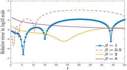
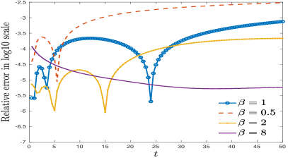
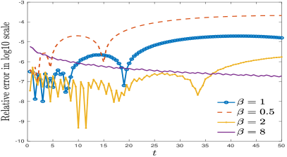
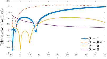
Here we provide an illustrative example to demonstrate the dynamical increments of projection error and the influences under different scaling factors. Considering

I(t)=0+y4γ1ϕ(y,t)dy,tϕ(y,t)=1y2ϕ(y,t),ϕ(y,0)=1,formulae-sequence𝐼𝑡superscriptsubscript0superscript𝑦4𝛾1italic-ϕ𝑦𝑡d𝑦formulae-sequence𝑡italic-ϕ𝑦𝑡1superscript𝑦2italic-ϕ𝑦𝑡italic-ϕ𝑦01I(t)=\int_{0}^{+\infty}y^{4\gamma-1}\phi(y,t)\textup{d}y,\quad\frac{\partial}{\partial t}\phi(y,t)=1-y^{2}\phi(y,t),\quad\phi(y,0)=1, (3.16)

the exact solution of dynamics is ϕ(y,t)=𝕖y2t+y2(1𝕖y2t)italic-ϕ𝑦𝑡superscript𝕖superscript𝑦2𝑡superscript𝑦21superscript𝕖superscript𝑦2𝑡\phi(y,t)=\mathbbm{e}^{-y^{2}t}+y^{-2}(1-\mathbbm{e}^{-y^{2}t}). Using Eq. (3.3) to evaluate the integral I(t)𝐼𝑡I(t), with M+1=500𝑀1500M+1=500, β=1𝛽1\beta=1 adopted as the reference, we can see in Figure 1 that the accuracy of the Laguerre-Gauss quadrature deteriorates in time evolution, regardless of the number of collocation points. After choosing a scaling factor β>1𝛽1\beta>1, one can observe a slight reduction of accuracy at the early stage, but the amplification of numerical errors can be considerably suppressed in time evolution, while further increasing β𝛽\beta may lead to larger truncation error. But overall, the dynamical increments of numerical errors can be alleviated. By contrast, β<1𝛽1\beta<1 will lead to a more severe increments of errors.
Refer to caption
(a) M+1=8𝑀18M+1=8, γ=0.1𝛾0.1\gamma=0.1.
Refer to caption
(b) M+1=32𝑀132M+1=32, γ=0.1𝛾0.1\gamma=0.1.
Refer to caption
(c) M+1=8𝑀18M+1=8, γ=0.001𝛾0.001\gamma=0.001.
Refer to caption
(d) M+1=32𝑀132M+1=32, γ=0.001𝛾0.001\gamma=0.001.
Figure 1: Numerical accuracy of the Laguerre-Gauss quadrature for the integral I(t)𝐼𝑡I(t) in (3.16). Numerical errors will be amplified in time evolution, regardless of the choice of M𝑀M. Choosing a scaling factor β>1𝛽1\beta>1 will suppress the increments, while β<1𝛽1\beta<1 will lead to a more severe amplification of numerical errors.

3.3 A splitting scheme

Finally, we illustrate the setting of our SMOS scheme. Although the operator y2dsuperscript𝑦2subscript𝑑-y^{2}\mathcal{I}_{d} breaks the Hamiltonian structure, the constant-Q wave equation can still be evolved efficiently by an appropriate operator splitting.

Eq. (2.14) are equivalent to

t(𝒗Φ[𝜺])=(𝒗Φ[𝜺])+𝒰(𝒗Φ[𝜺]),𝑡matrix𝒗Φdelimited-[]𝜺matrix𝒗Φdelimited-[]𝜺𝒰matrix𝒗Φdelimited-[]𝜺\frac{\partial}{\partial t}\begin{pmatrix}\bm{v}\\ \Phi[\bm{\varepsilon}]\end{pmatrix}=\mathcal{L}\begin{pmatrix}\bm{v}\\ \Phi[\bm{\varepsilon}]\end{pmatrix}+\mathcal{U}\begin{pmatrix}\bm{v}\\ \Phi[\bm{\varepsilon}]\end{pmatrix}, (3.17)

where the operators \mathcal{L} and 𝒰𝒰\mathcal{U} are given by

(𝒗Φ[𝜺])=(001y2d)(𝒗Φ[𝜺])matrix𝒗Φdelimited-[]𝜺matrix00subscript1superscript𝑦2subscript𝑑matrix𝒗Φdelimited-[]𝜺\mathcal{L}\begin{pmatrix}\bm{v}\\ \Phi[\bm{\varepsilon}]\end{pmatrix}=\begin{pmatrix}0&0\\ \mathcal{L}_{1}&-y^{2}\mathcal{I}_{d}\end{pmatrix}\begin{pmatrix}\bm{v}\\ \Phi[\bm{\varepsilon}]\end{pmatrix} (3.18)

and

𝒰(𝒗Φ[𝜺])=(03200)(𝒗Φ[𝜺])+(𝒇0).𝒰matrix𝒗Φdelimited-[]𝜺matrix0subscript3subscript200matrix𝒗Φdelimited-[]𝜺matrix𝒇0\mathcal{U}\begin{pmatrix}\bm{v}\\ \Phi[\bm{\varepsilon}]\end{pmatrix}=\begin{pmatrix}0&\mathcal{L}_{3}\circ\mathcal{L}_{2}\\ 0&0\end{pmatrix}\begin{pmatrix}\bm{v}\\ \Phi[\bm{\varepsilon}]\end{pmatrix}+\begin{pmatrix}\bm{f}\\ 0\end{pmatrix}. (3.19)

Suppose the time interval [0,T]0𝑇[0,T] is divided into N𝑁N steps, with spacing Δt=T/NΔ𝑡𝑇𝑁\Delta t=T/N, tn=nΔtsubscript𝑡𝑛𝑛Δ𝑡t_{n}=n\Delta t. Now we can use the Strang splitting

exp(t(+𝒰)=[exp(Δt2𝒰)exp(Δt)exp(Δt2𝒰)]n+𝒪((Δt)3)\exp(t(\mathcal{L}+\mathcal{U})=\left[\exp(\frac{\Delta t}{2}\mathcal{U})\circ\exp(\Delta t\mathcal{L})\circ\exp(\frac{\Delta t}{2}\mathcal{U})\right]^{n}+\mathcal{O}((\Delta t)^{3}) (3.20)

The splitting procedure is rather appealing as the exact solution of each subproblem can be readily obtained. For the first subproblem (3.18), the exact solution reads that

{𝒗(𝒙,t)=𝒗(𝒙,tn),Φ[𝜺](𝒙,y,t)=𝕖y2(ttn)Φ[𝜺](𝒙,y,tn)+1y2(1𝕖y2(ttn))1𝒗(𝒙,tn).\left\{\begin{split}&\bm{v}(\bm{x},t)=\bm{v}(\bm{x},t_{n}),\\ &\Phi[\bm{\varepsilon}](\bm{x},y,t)=\mathbbm{e}^{-y^{2}(t-t_{n})}\Phi[\bm{\varepsilon}](\bm{x},y,t_{n})+\frac{1}{y^{2}}(1-\mathbbm{e}^{-y^{2}(t-t_{n})})\mathcal{L}_{1}\bm{v}(\bm{x},t_{n}).\end{split}\right. (3.21)

This avoids the numerical stiffness caused by sufficiently large y2superscript𝑦2y^{2} and additional numerical errors in solving the auxiliary relaxed dynamics (2.9).

For the second subproblem (3.19), the exact solution reads that

{𝒗(𝒙,t)=𝒗(𝒙,tn)+(ttn)32Φ[𝜺](𝒙,y,tn)+tnt𝒇(𝒙,s)ds,Φ[𝜺](𝒙,y,t)=Φ[𝜺](𝒙,y,tn).\left\{\begin{split}&\bm{v}(\bm{x},t)=\bm{v}(\bm{x},t_{n})+(t-t_{n})\mathcal{L}_{3}\circ\mathcal{L}_{2}\Phi[\bm{\varepsilon}](\bm{x},y,t_{n})+\int_{t_{n}}^{t}\bm{f}(\bm{x},s)\textup{d}s,\\ &\Phi[\bm{\varepsilon}](\bm{x},y,t)=\Phi[\bm{\varepsilon}](\bm{x},y,t_{n}).\end{split}\right. (3.22)

The SMOS scheme for unidimensional constant-Q wave equation is given in Algorithm 1, and its generalization to higher-dimensional case is straightforward. Here the strain tensor is added for physical meaning and a more concise description of the algorithm. Compared with the Strang splitting scheme for elastic wave equation, the only difference lies in the second step and there is no additional cost in evaluating the gradients of velocity vectors and stress tensors.

Algorithm 1 Short-memory operator splitting (SMOS) scheme

Input: The order M𝑀M of Laguerre-Gauss quadrature, the scaling factor β𝛽\beta

  • 1.

    Half-step update of velocity (vector):

    𝒗(𝒙,tn+12)=𝒗(𝒙,tn)+Δt23σ(𝒙,tn)+tntn+Δt2𝒇(𝒙,s)ds.𝒗𝒙subscript𝑡𝑛12𝒗𝒙subscript𝑡𝑛Δ𝑡2subscript3𝜎𝒙subscript𝑡𝑛superscriptsubscriptsubscript𝑡𝑛subscript𝑡𝑛Δ𝑡2𝒇𝒙𝑠d𝑠\bm{v}(\bm{x},t_{n+\frac{1}{2}})=\bm{v}(\bm{x},t_{n})+\frac{\Delta t}{2}\mathcal{L}_{3}\sigma(\bm{x},t_{n})+\int_{t_{n}}^{t_{n}+\frac{\Delta t}{2}}\bm{f}(\bm{x},s)\textup{d}s.
  • 2.

    Full-step update of stress (tensor), with y~jsubscript~𝑦𝑗\tilde{y}_{j} short for yj(4γ1,β)superscriptsubscript𝑦𝑗4𝛾1𝛽y_{j}^{(4\gamma-1,\beta)}:

    {𝝈(𝒙,tn+1)=ρ(𝒙)2Csin(2πγ)πj=0Mωj(4γ1,β)𝕖βy~jΦ[𝜺](𝒙,y~j,t),Φ[𝜺](𝒙,y~j,tn+1)=𝕖y~j2ΔtΦ[𝜺](𝒙,y~j,tn)+1y~j2(1𝕖y~j2Δt)1𝒗(𝒙,tn+12).\left\{\begin{split}&\bm{\sigma}(\bm{x},t_{n+1})=\rho(\bm{x})\frac{2C\sin(2\pi\gamma)}{\pi}\sum_{j=0}^{M}\omega_{j}^{(4\gamma-1,\beta)}\mathbbm{e}^{\beta\tilde{y}_{j}}\Phi[\bm{\varepsilon}](\bm{x},\tilde{y}_{j},t),\\ &\Phi[\bm{\varepsilon}](\bm{x},\tilde{y}_{j},t_{n+1})=\mathbbm{e}^{-\tilde{y}_{j}^{2}\Delta t}\Phi[\bm{\varepsilon}](\bm{x},\tilde{y}_{j},t_{n})+\frac{1}{\tilde{y}_{j}^{2}}(1-\mathbbm{e}^{-\tilde{y}_{j}^{2}\Delta t})\mathcal{L}_{1}\bm{v}(\bm{x},t_{n+\frac{1}{2}}).\end{split}\right.
  • 3.

    Half-step update of velocity (vector):

    𝒗(𝒙,tn+1)=𝒗(𝒙,tn+12)+Δt23σ(𝒙,tn+1)+tn+12tn+12+Δt2𝒇(𝒙,s)ds.𝒗𝒙subscript𝑡𝑛1𝒗𝒙subscript𝑡𝑛12Δ𝑡2subscript3𝜎𝒙subscript𝑡𝑛1superscriptsubscriptsubscript𝑡𝑛12subscript𝑡𝑛12Δ𝑡2𝒇𝒙𝑠d𝑠\bm{v}(\bm{x},t_{n+1})=\bm{v}(\bm{x},t_{n+\frac{1}{2}})+\frac{\Delta t}{2}\mathcal{L}_{3}\sigma(\bm{x},t_{n+1})+\int_{t_{n+\frac{1}{2}}}^{t_{n+\frac{1}{2}}+\frac{\Delta t}{2}}\bm{f}(\bm{x},s)\textup{d}s.

The gradient operators 1subscript1\mathcal{L}_{1} and 3subscript3\mathcal{L}_{3} can be solved by the standard staggered-grid pseudo-spectral method [21, 38], and the integration of source term can be either tackled by the Gauss quadrature, or simply by the mid-point quadrature

tn+12tn+12+Δt2𝒇(𝒙,s)dsΔt2(𝒇(𝒙,tn+12)+𝒇(𝒙,tn+12+Δt2)).superscriptsubscriptsubscript𝑡𝑛12subscript𝑡𝑛12Δ𝑡2𝒇𝒙𝑠d𝑠Δ𝑡2𝒇𝒙subscript𝑡𝑛12𝒇𝒙subscript𝑡𝑛12Δ𝑡2\int_{t_{n+\frac{1}{2}}}^{t_{n+\frac{1}{2}}+\frac{\Delta t}{2}}\bm{f}(\bm{x},s)\textup{d}s\approx\frac{\Delta t}{2}\left(\bm{f}(\bm{x},t_{n+\frac{1}{2}})+\bm{f}(\bm{x},t_{n+\frac{1}{2}}+\frac{\Delta t}{2})\right). (3.23)

For two-dimensional case, a trick is adopted to reduce memory variables. Suppose γPγSsubscript𝛾𝑃subscript𝛾𝑆\gamma_{P}\leq\gamma_{S} so that y4γS4γPsuperscript𝑦4subscript𝛾𝑆4subscript𝛾𝑃y^{4\gamma_{S}-4\gamma_{P}} is not singular, then we have

0+y4γS1Φ[𝜺](x,z,y,t)dy=0+y4γP1y4γS4γPΦ[𝜺](x,z,y,t)dy,superscriptsubscript0superscript𝑦4subscript𝛾𝑆1Φdelimited-[]𝜺𝑥𝑧𝑦𝑡d𝑦superscriptsubscript0superscript𝑦4subscript𝛾𝑃1superscript𝑦4subscript𝛾𝑆4subscript𝛾𝑃Φdelimited-[]𝜺𝑥𝑧𝑦𝑡d𝑦\int_{0}^{+\infty}y^{4\gamma_{S}-1}\Phi[\bm{\varepsilon}](x,z,y,t)\textup{d}y=\int_{0}^{+\infty}y^{4\gamma_{P}-1}y^{4\gamma_{S}-4\gamma_{P}}\Phi[\bm{\varepsilon}](x,z,y,t)\textup{d}y,

and the Laguerre functions can be chosen as m(4γP1,β)(y)superscriptsubscript𝑚4subscript𝛾𝑃1𝛽𝑦\mathscr{L}_{m}^{(4\gamma_{P}-1,\beta)}(y), instead of m(4γS1,β)(y)superscriptsubscript𝑚4subscript𝛾𝑆1𝛽𝑦\mathscr{L}_{m}^{(4\gamma_{S}-1,\beta)}(y).

4 Numerical experiments

In this section, numerical experiments on 1-D diffusive wave equation and 2-D constant-Q wave equation are performed to give a thorough benchmark on the SMOS scheme. Our concern includes an investigation of the convergence with respect to the time step ΔtΔ𝑡\Delta t, number of spatial collocation points Nxsubscript𝑁𝑥N_{x} and the memory length M𝑀M, as well as the scaling factor β𝛽\beta. Afterward we present the benchmarks on 2-D constant-Q viscoelastic wave equation and give a detailed study of convergence with respect to the memory length MP=MS=Msubscript𝑀𝑃subscript𝑀𝑆𝑀M_{P}=M_{S}=M and the effect of scaling.

For spatial discretization, we adopt the staggered-grid pseudo-spectral method in discretizing the spatial derivatives, which is suggested to improve both stability and accuracy in applications of fluid dynamics or elasticity [38]. Suppose the finite computational domain is [xmin,xmax]subscript𝑥subscript𝑥[x_{\min},x_{\max}] in each dimension, then the staggered grid mesh is xmin=x0<x1/2<x1<x3/2<<xN1<xN1/2<xN=xmaxsubscript𝑥subscript𝑥0subscript𝑥12subscript𝑥1subscript𝑥32subscript𝑥𝑁1subscript𝑥𝑁12subscript𝑥𝑁subscript𝑥x_{\min}=x_{0}<x_{1/2}<x_{1}<x_{3/2}<\dots<x_{N-1}<x_{N-1/2}<x_{N}=x_{\max}, where xj=xmin+jΔxsubscript𝑥𝑗subscript𝑥𝑗Δ𝑥x_{j}=x_{\min}+j\Delta x, xj+1/2=xmin+(j+1/2)Δxsubscript𝑥𝑗12subscript𝑥𝑗12Δ𝑥x_{j+1/2}=x_{\min}+(j+1/2)\Delta x with the spacing Δx=xmaxxminNΔ𝑥subscript𝑥subscript𝑥𝑁\Delta x=\frac{x_{\max}-x_{\min}}{N}. For 1-D problem, the grid mesh for strain σ𝜎\sigma and velocity v𝑣v are {xj}j=0N1superscriptsubscriptsubscript𝑥𝑗𝑗0𝑁1\{x_{j}\}_{j=0}^{N-1} and {xj+1/2}j=0N1superscriptsubscriptsubscript𝑥𝑗12𝑗0𝑁1\{x_{j+1/2}\}_{j=0}^{N-1}, respectively, while that in the 2-D problem can be found in [38]. In order to preclude the errors induced by the artificial boundary condition [18, 23], we simply enlarge the computational domain to avoid the artificial wave reflection.

To measure the numerical errors, we adopt the relative Lsuperscript𝐿L^{\infty}-error subscript\mathcal{E}_{\infty} as the performance metric.

[φ](t)=max𝒙𝒳|φnum(𝒙,t)φref(𝒙,t)|max𝒙𝒳|φref(𝒙,t)|,subscriptdelimited-[]𝜑𝑡subscript𝒙𝒳subscript𝜑num𝒙𝑡subscript𝜑ref𝒙𝑡subscript𝒙𝒳subscript𝜑ref𝒙𝑡\mathcal{E}_{\infty}[{\varphi}](t)=\frac{\max_{\bm{x}\in\mathcal{X}}|\varphi_{\textup{num}}(\bm{x},t)-{\varphi}_{\textup{ref}}(\bm{x},t)|}{\max_{\bm{x}\in\mathcal{X}}|{\varphi}_{\textup{ref}}(\bm{x},t)|}, (4.1)

where φ𝜑\varphi is a scalar quantity. For 1-D problem, φ(x,t)=v(x,t)𝜑𝑥𝑡𝑣𝑥𝑡\varphi(x,t)=v(x,t) and for 2-D problem, φ(𝒙,t)=u3(𝒙,t)𝜑𝒙𝑡subscript𝑢3𝒙𝑡\varphi(\bm{x},t)=u_{3}(\bm{x},t) or σ13(𝒙,t)subscript𝜎13𝒙𝑡\sigma_{13}(\bm{x},t).

The subroutines GEN_LAGUERRE_RULE [39] is used to obtain nodes and weights for the generalized Laguerre-Gauss quadrature. All the simulations performed via MATLAB (1-D) or Fortran (2-D) implementations run on the platform: AMD Threadripper 1920X (3.50GHz, 32MB Cache, 12 Cores, 24 Threads) with 128GB Memory. The parallelization for 2-D problem is realized by the OpenMP library using up to 24 threads.

4.1 1-D diffusive wave equation without source term

The first benchmark is to solve the diffusive wave equation (2.20) with ρ1𝜌1\rho\equiv 1 and C=1𝐶1C=1. The initial condition is set as

v(x,t)|t=0+evaluated-at𝑣𝑥𝑡𝑡superscript0\displaystyle v(x,t)|_{t=0^{+}} =𝕖x2,tv(x,t)|t=0+=0,formulae-sequenceabsentsuperscript𝕖superscript𝑥2evaluated-at𝑡𝑣𝑥𝑡𝑡superscript00\displaystyle=\mathbbm{e}^{-x^{2}},\quad\frac{\partial}{\partial t}v(x,t)|_{t=0^{+}}=0,\quad <x<,𝑥\displaystyle-\infty<x<\infty, (4.2)
σ(x,t)|t=0+evaluated-at𝜎𝑥𝑡𝑡superscript0\displaystyle\sigma(x,t)|_{t=0^{+}} =Dt2γCε(x,t)|t=0+=0,absentevaluated-atsubscriptsuperscriptsubscript𝐷𝑡2𝛾𝐶𝜀𝑥𝑡𝑡superscript00\displaystyle={{}_{C}}D_{t}^{2\gamma}\varepsilon(x,t)|_{t=0^{+}}=0,\quad <x<,𝑥\displaystyle-\infty<x<\infty, (4.3)
Φ(x,y,t)|t=0+evaluated-atΦ𝑥𝑦𝑡𝑡superscript0\displaystyle\Phi(x,y,t)|_{t=0^{+}} =Γ(12γ)𝕖y2σ(x,t)|t=0+=0,absentevaluated-atΓ12𝛾superscript𝕖superscript𝑦2𝜎𝑥𝑡𝑡superscript00\displaystyle=\Gamma(1-2\gamma)\mathbbm{e}^{-y^{2}}\sigma(x,t)|_{t=0^{+}}=0,\quad <x,y<,formulae-sequence𝑥𝑦\displaystyle-\infty<x,y<\infty, (4.4)

and v(±,t)=0𝑣plus-or-minus𝑡0v(\pm\infty,t)=0. The initial strain is derived by xε(x,t)|t=0+=tv(x,t)|t=0+evaluated-at𝑥𝜀𝑥𝑡𝑡superscript0evaluated-at𝑡𝑣𝑥𝑡𝑡superscript0\frac{\partial}{\partial x}\varepsilon(x,t)|_{t=0^{+}}=\frac{\partial}{\partial t}v(x,t)|_{t=0^{+}}.

In order to provide a reasonable reference for small γ𝛾\gamma, we utilize the intriguing spectral approximation to the exact solution of (2.21). Let s=Ct1γ𝑠𝐶superscript𝑡1𝛾s=\sqrt{C}t^{1-\gamma}, then

ε(x,t)=120+M1γ(y)[𝕖(xsy)2+𝕖(x+sy)2]dy{12j=0Myωj(0,1s)𝕖yj(0,1)M1γ(yj(0,1s))[𝕖(xsyj(0,1s))2+𝕖(x+syj(0,1s))2],t<1,12sj=0MyωjHM1γ(xyjHs),t1,\begin{split}\varepsilon(x,t)&=\frac{1}{2}\int_{0}^{+\infty}M_{1-\gamma}(y)\left[\mathbbm{e}^{-(x-sy)^{2}}+\mathbbm{e}^{(x+sy)^{2}}\right]\textup{d}y\\ &\approx\left\{\begin{split}&\frac{1}{2}\sum_{j=0}^{M_{y}}\omega_{j}^{(0,\frac{1}{s})}\mathbbm{e}^{y_{j}^{(0,1)}}M_{1-\gamma}(y_{j}^{(0,\frac{1}{s})})\left[\mathbbm{e}^{-(x-sy_{j}^{(0,\frac{1}{s})})^{2}}+\mathbbm{e}^{(x+sy_{j}^{(0,\frac{1}{s})})^{2}}\right],~{}~{}t<1,\\ &\frac{1}{2s}\sum_{j=0}^{M_{y}}\omega_{j}^{H}M_{1-\gamma}\left(\frac{x-y_{j}^{H}}{s}\right),~{}~{}t\geq 1,\end{split}\right.\end{split}

which can be approximated by either the Laguerre-Gauss quadrature or the Hermite-Gauss quadrature, with yjHsuperscriptsubscript𝑦𝑗𝐻y_{j}^{H} and ωjHsuperscriptsubscript𝜔𝑗𝐻\omega_{j}^{H} the collocations points and weights of the Hermite-Gauss quadrature, respectively. The calculation of the Mainardi function is entirely not trivial. We try to realize it by combining the generalized Laguerre-Gauss quadrature and its asymptotic expansion, and details are put in A.

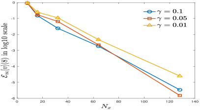
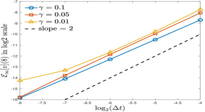
The computational domain is 𝒳=[xmin,xmax]=[15,15]𝒳subscript𝑥subscript𝑥1515\mathcal{X}=[x_{\min},x_{\max}]=[-15,15]. The final time is T=8𝑇8T=8. Other parameters include: the fractional order γ=0.1,0.05,0.01𝛾0.10.050.01\gamma=0.1,0.05,0.01, the time step Δt=24,25,26,27,28Δ𝑡superscript24superscript25superscript26superscript27superscript28\Delta t=2^{-4},2^{-5},2^{-6},2^{-7},2^{-8}, the memory length M+1=4,8,16,32,64𝑀148163264M+1=4,8,16,32,64 and Nx=8,16,32,64,128subscript𝑁𝑥8163264128N_{x}=8,16,32,64,128. In order to evaluate the performance of SMOS, we first investigate the convergence with ΔtΔ𝑡\Delta t (with Nx=128subscript𝑁𝑥128N_{x}=128, M+1=256𝑀1256M+1=256 fixed), Nxsubscript𝑁𝑥N_{x} (with Δt=104Δ𝑡superscript104\Delta t=10^{-4}, M+1=256𝑀1256M+1=256 fixed) as presented in Figure 2.

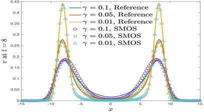
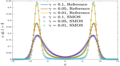
A visualization of the velocity propagation under different memory lengths (with Δt=104Δ𝑡superscript104\Delta t=10^{-4}, Nx=128subscript𝑁𝑥128N_{x}=128, β=1𝛽1\beta=1) is presented in Figure 3. The velocity splits into two branches, each of which propagates in opposite directions and reaches the centers x=±8𝑥plus-or-minus8x=\pm 8 at T=8𝑇8T=8, respectively. In contrast to the elastic case, the attenuation of wave front can be observed as the height of waveform decreases, and the attenuation level becomes more evident for larger γ𝛾\gamma.

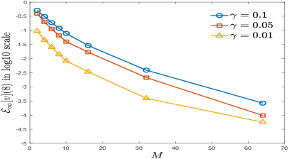
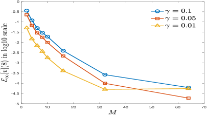
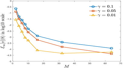
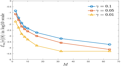
The main goal is to investigate how the scaling factor β𝛽\beta influences the accuracy under the parameters: Δt=104Δ𝑡superscript104\Delta t=10^{-4}, Nx=128subscript𝑁𝑥128N_{x}=128 and fixed M𝑀M. The maximal errors and averaged computational time are recorded in Table 1. The convergence with respect to M𝑀M is presented in Figure 4. From the results, we can make the following observations.
Refer to caption
(a) Convergence w.r.t ΔtΔ𝑡\Delta t.
Refer to caption
(b) Convergence w.r.t. Nxsubscript𝑁𝑥N_{x}.
Figure 2: 1-D diffusive wave propagation: The convergence with respect to time step ΔtΔ𝑡\Delta t and number of spatial collocation points Nxsubscript𝑁𝑥N_{x}. For different γ𝛾\gamma, the second-order convergence with ΔtΔ𝑡\Delta t is always observed, which coincides with the theoretical value in the Strang splitting. Meanwhile, the spectral convergence is achieved in the spatial direction.
Refer to caption
(a) M+1=4𝑀14M+1=4.
Refer to caption
(b) M+1=8𝑀18M+1=8.
Refer to caption
(c) M+1=16𝑀116M+1=16.
Refer to caption
(d) M+1=256𝑀1256M+1=256.
Figure 3: 1-D diffusive wave propagation: The propagation of velocity at T=8𝑇8T=8, under different memory M+1𝑀1M+1. The velocity splits into two parts and the attenuation of waveform in the propagation is clearly observed. When M𝑀M is small, numerical solutions slightly deviate the exact ones, but the errors can be evidently suppressed when M+1=16𝑀116M+1=16.
Refer to caption
(a) β=0.5𝛽0.5\beta=0.5.
Refer to caption
(b) β=1𝛽1\beta=1.
Refer to caption
(c) β=1.5𝛽1.5\beta=1.5.
Refer to caption
(d) β=2𝛽2\beta=2.
Figure 4: 1-D diffusive wave propagation: The convergence with respect to M𝑀M, under different scaling factors β𝛽\beta. SMOS convergences rapidly when M+132𝑀132M+1\leq 32, but the trend slows down for larger M𝑀M. When γ𝛾\gamma is small, only a few memory variables can accurately seize the major contribution.
Table 1: 1-D diffusive wave equation: [v]subscriptdelimited-[]𝑣\mathcal{E}_{\infty}[v] at T=8𝑇8T=8 and the averaged computational time, with Δt=104Δ𝑡superscript104\Delta t=10^{-4} and Nx=128subscript𝑁𝑥128N_{x}=128.

γ𝛾\gamma M𝑀M β𝛽\beta 0.5 1 1.5 2 4 8 time(s) 0.10.10.1 7 1.188E-01 2.967E-02 1.172E-02 6.103E-03 2.061E-02 6.896E-02 4.08 15 1.399E-02 3.908E-03 1.274E-03 1.971E-03 6.042E-03 1.882E-02 4.27 31 3.903E-03 2.626E-04 3.836E-04 6.096E-04 1.857E-03 5.681E-03 4.82 63 2.659E-04 6.159E-05 9.836E-05 1.914E-04 5.853E-04 1.783E-03 5.75 0.050.050.05 7 6.632E-02 1.774E-02 5.383E-03 3.877E-03 1.394E-02 5.150E-02 4.11 15 2.905E-02 2.157E-03 5.959E-04 1.005E-03 3.522E-03 1.246E-02 4.29 31 2.126E-03 9.896E-05 1.575E-04 2.660E-04 9.332E-04 3.269E-03 4.84 63 9.718E-05 1.870E-05 3.133E-05 7.110E-05 2.535E-04 8.883E-04 5.78 0.010.010.01 7 1.399E-02 3.596E-03 8.915E-04 8.503E-04 3.430E-03 1.343E-02 4.12 15 3.418E-03 4.047E-04 8.091E-05 1.513E-04 7.348E-04 3.008E-03 4.28 31 3.924E-04 5.009E-05 4.578E-05 5.039E-05 1.350E-04 6.680E-04 4.87 63 5.606E-05 5.461E-05 5.207E-05 4.733E-05 6.596E-05 1.851E-04 5.77

  • (1)

    The second-order convergence with respect to ΔtΔ𝑡\Delta t is clearly observed and accords with the theoretical value perfectly. In addition, the spectral convergence of the staggered pseudo-spectral method is also verified.

  • (2)

    As presented in Figure 4, the spectral convergence for the Laguerre spectral method is clearly observed before M+132𝑀132M+1\leq 32. But after the pre-asymptotic range, the Laguerre spectral approximation converges only algebraically, instead of exponentially. That accounts for the observation that further increasing the memory length might not improve the accuracy when γ=0.01𝛾0.01\gamma=0.01. For sufficiently small γ𝛾\gamma (e.g., γ=0.01𝛾0.01\gamma=0.01), using only a few nodes can produce accurate results, as shown in Figure 3. This provides some evidence to validate our short-memory principle as too many memory variables might not necessarily bring in significant improvement in accuracy.

  • (3)

    The effect of scaling is shown in Figure 4 and Table 1. Even without source term, for relatively small M+116𝑀116M+1\leq 16, the numerical results under β=2𝛽2\beta=2 usually outperform those without scaling, whereas choosing β<1𝛽1\beta<1 diminishes the numerical accuracy. Such result also coincides with our theoretical prediction in Proposition 1. In other words, it manifests the importance of choosing an appropriate scaling factor in SMOS as it may indeed significantly enhance the accuracy, without introducing additional numerical cost. However, too large scaling factor is not recommended as it may lead to larger truncation errors.

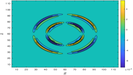
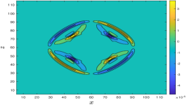
4.2 2-D Constant-Q P- and S-wave modeling with source term

For 2-D problem, we consider the wave propagation from a horizontal source function with Ricker-type wavelet history,

f1(x,z,t)=A(x,z)fr(t),f3(x,z,t)=0,\begin{split}f_{1}(x,z,t)=A(x,z)f_{r}(t),\quad f_{3}(x,z,t)=0,\end{split} (4.5)

where the amplitude function A(x,z)𝐴𝑥𝑧A(x,z) is simply set as a Gaussian profile centered at (x0,z0)subscript𝑥0subscript𝑧0(x_{0},z_{0}),

A(x,z)=exp((xx0)2/2)exp((zz0)2/2)𝐴𝑥𝑧superscript𝑥subscript𝑥022superscript𝑧subscript𝑧022A(x,z)=\exp(-{(x-x_{0})^{2}}/{2})\exp(-{(z-z_{0})^{2}}/{2}) (4.6)

and the Ricker wavelet is given by

fr(t)=(12(πfP(tdr)2)exp((πfP(tdr))2),f_{r}(t)=(1-2(\pi f_{P}(t-d_{r})^{2})\exp(-(\pi f_{P}(t-d_{r}))^{2}), (4.7)

where fPsubscript𝑓𝑃f_{P} is the peak frequency and drsubscript𝑑𝑟d_{r} is the temporal delay.

The medium is supposed to be in equilibrium at t=0𝑡0t=0, namely, stress tensor and velocity vector are set to zero everywhere in the medium [2].

v1(x,z,t)|t=0+=v3(x,z,t)|t=0+=0,evaluated-atsubscript𝑣1𝑥𝑧𝑡𝑡superscript0evaluated-atsubscript𝑣3𝑥𝑧𝑡𝑡superscript00\displaystyle v_{1}(x,z,t)|_{t=0^{+}}=v_{3}(x,z,t)|_{t=0^{+}}=0, (4.8)
σ11(x,z,t)|t=0+=σ33(x,z,t)|t=0+=σ13(x,z,t)|t=0+=0,evaluated-atsubscript𝜎11𝑥𝑧𝑡𝑡superscript0evaluated-atsubscript𝜎33𝑥𝑧𝑡𝑡superscript0evaluated-atsubscript𝜎13𝑥𝑧𝑡𝑡superscript00\displaystyle\sigma_{11}(x,z,t)|_{t=0^{+}}=\sigma_{33}(x,z,t)|_{t=0^{+}}=\sigma_{13}(x,z,t)|_{t=0^{+}}=0, (4.9)
Φ11(x,z,y,t)|t=0+=Φ33(x,z,y,t)|t=0+=Φ13(x,z,y,t)|t=0+=0.evaluated-atsubscriptΦ11𝑥𝑧𝑦𝑡𝑡superscript0evaluated-atsubscriptΦ33𝑥𝑧𝑦𝑡𝑡superscript0evaluated-atsubscriptΦ13𝑥𝑧𝑦𝑡𝑡superscript00\displaystyle\Phi_{11}(x,z,y,t)|_{t=0^{+}}=\Phi_{33}(x,z,y,t)|_{t=0^{+}}=\Phi_{13}(x,z,y,t)|_{t=0^{+}}=0. (4.10)

Two typical groups of parameters are collected in Table 2, including wave velocities, density and quality factors for different medium found in [7], and the reference frequency ω0subscript𝜔0\omega_{0} is about 2π×1002𝜋1002\pi\times 100Hz. Thus the constants CPsubscript𝐶𝑃C_{P} and CSsubscript𝐶𝑆C_{S} can be evaluated by Eq. (2.5).

Table 2: Reference wave velocities, density and quality factors

Medium cPsubscript𝑐𝑃c_{P} (km/s) cSsubscript𝑐𝑆c_{S} (km/s) ρ𝜌\rho (g/cm3superscriptcm3\textup{cm}^{3}) QPsubscript𝑄𝑃Q_{P} QSsubscript𝑄𝑆Q_{S} γPsubscript𝛾𝑃\gamma_{P} γSsubscript𝛾𝑆\gamma_{S} 1 3.2 1.85 2.5 32 10 0.0099 0.0317 2 3.2 1.85 2.5 100 50 0.0032 0.0064

The computational domain is 𝒳=[0,120]×[0,120]𝒳01200120\mathcal{X}=[0,120]\times[0,120] with Nx=Nz=512subscript𝑁𝑥subscript𝑁𝑧512N_{x}=N_{z}=512. The parameters for the initial source term are fP=100subscript𝑓𝑃100f_{P}=100Hz and dr=60subscript𝑑𝑟60d_{r}=60. The time step is Δt=0.001Δ𝑡0.001\Delta t=0.001 and the final instant is T=15𝑇15T=15. The memory length of the reference solution is MP=MS=499subscript𝑀𝑃subscript𝑀𝑆499M_{P}=M_{S}=499. Different groups of memory length M𝑀M and scaling factor β𝛽\beta are considered: MP=MS=7,15,31,63formulae-sequencesubscript𝑀𝑃subscript𝑀𝑆7153163M_{P}=M_{S}=7,15,31,63, β=0.6,1,2,8,16,32𝛽0.61281632\beta=0.6,1,2,8,16,32. For the sake of comparison, we also calculate the elastic modeling under cP=3.2subscript𝑐𝑃3.2c_{P}=3.2, cS=1.85subscript𝑐𝑆1.85c_{S}=1.85, ρ=2.5𝜌2.5\rho=2.5.

The wave attenuation phenomena are much more complicated in 2-D case. A comparison among the displacement u3subscript𝑢3u_{3} in z𝑧z-direction and the (xz)𝑥𝑧(xz)-component σ13subscript𝜎13\sigma_{13} of the stress tensor is plotted in Figures 5 and 6, respectively. The difference between the viscoelastic wave propagation and the elastic counterpart is transparent. Since the Ricker wavelet source has two peaks at t=0𝑡0t=0 and t=0.24𝑡0.24t=0.24, two wave fronts are observed in the elastic media and they propagate independently. By contrast, two wave fronts in the viscoelastic media seem to stick together due to the time-lag effect (the power creep) in the stress-strain relation. One can see that the wave attenuation is more evident in the first viscoelastic media and the height of waveform decreases considerably in the time evolution. In the second viscoelastic media, although the shapes of wave fronts change a lot, there is only a slight reduction in the height due to smaller loss of energy.
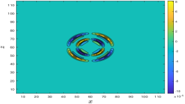
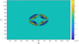
Refer to caption
Refer to caption
Refer to caption
(a) t=5𝑡5t=5.
Refer to caption
Refer to caption
Refer to caption
(b) t=10𝑡10t=10.
Refer to caption
Refer to caption
Refer to caption
(c) t=15𝑡15t=15.
Figure 5: 2-D constant-Q wave propagation: Displacement u3subscript𝑢3u_{3}. Left: elastic modeling, mid: viscoelastic modeling with quality factors QP=32subscript𝑄𝑃32Q_{P}=32, QS=10subscript𝑄𝑆10Q_{S}=10, right: viscoelastic modeling with quality factors QP=100subscript𝑄𝑃100Q_{P}=100, QS=50subscript𝑄𝑆50Q_{S}=50.
Refer to caption
Refer to caption
Refer to caption
(a) t=5𝑡5t=5.
Refer to caption
Refer to caption
Refer to caption
(b) t=10𝑡10t=10.
Refer to caption
Refer to caption
Refer to caption
(c) t=15𝑡15t=15.
Figure 6: 2-D constant-Q wave propagation: Stress σ13subscript𝜎13\sigma_{13}. Left: elastic modeling, mid: viscoelastic modeling with quality factors QP=32subscript𝑄𝑃32Q_{P}=32, QS=10subscript𝑄𝑆10Q_{S}=10, right: viscoelastic modeling with quality factors QP=100subscript𝑄𝑃100Q_{P}=100, QS=50subscript𝑄𝑆50Q_{S}=50.

For 2-D constant-Q wave equation under QP=32subscript𝑄𝑃32Q_{P}=32, QS=10subscript𝑄𝑆10Q_{S}=10, we focus on the study on the dynamical increments of numerical errors, as presented in Figure 7 associated a validation on the convergence of memory length MP=MS=Msubscript𝑀𝑃subscript𝑀𝑆𝑀M_{P}=M_{S}=M, and how the scaling technique ameliorates such problem. The numerical errors under different scaling factors and the averaged computational time are collected in Table 3. A visualization of the effect of scaling is presented in Figure 8. According to the results, we have the following observations.

  • (1)

    Although the spectral convergence of the Laguerre-Gauss quadrature is validated, the dynamical increments of projection errors is still observed in Figure 7. Compared with Figure 4, the reduction of accuracy is more evident because of the non-decay property of the source term. This observation coincides with our theoretical prediction.

  • (2)

    With appropriate scaling technique, the dynamical increments of numerical errors can be dramatically alleviated, albeit not eliminated. One can see in Table 3 that a large scaling factor β>1𝛽1\beta>1 may considerably enhance the numerical accuracy under the prescribed memory length without additional memory requirement or arithmetic complexity, while β<1𝛽1\beta<1 may even lead to a reduction in accuracy. In practice, β𝛽\beta should be chosen large enough in order to suppress the amplification induced by the source term (see M=32,β=16formulae-sequence𝑀32𝛽16M=32,\beta=16), but too large β𝛽\beta is still not recommended as the truncation errors are augmented.

  • (3)

    In Figure 8, we compare the unscaled and scaled results of u3subscript𝑢3u_{3} under M=32𝑀32M=32. Actually, the profile of wave propagation is very similar. The difference mainly lies in the height of waveforms as inadequate memory variables may underestimate the contribution of the singular integral and cause artificial loss of energy. Fortunately simply choosing a scaling factor β>1𝛽1\beta>1 can dramatically alleviate this problem.

  • (4)

    We can see in Table 7 that under M=32𝑀32M=32 and β=16𝛽16\beta=16, SMOS can achieve a relative Lsuperscript𝐿L^{\infty}-error about 2%4%percent2percent42\%-4\% at final instant T=15𝑇15T=15, and save about 82%percent8282\% computational time and 97%percent9797\% memory storage compared to M+1=500𝑀1500M+1=500. The memory length can be even shortened for smaller γ𝛾\gamma.

Refer to caption
(a) Convergence w.r.t. M𝑀M.
Refer to caption
(b) Dynamical errors in u3subscript𝑢3u_{3}.
Refer to caption
(c) Dynamical errors in σ13subscript𝜎13\sigma_{13}.
Figure 7: 2-D constant-Q wave propagation: The dynamical errors under different memory lengths M𝑀M. Although the spectral accuracy of the Laguerre-Gauss quadrature is verified, the dynamical increments of projection errors are clearly observed, regardless of choice of M𝑀M.
Refer to caption
(a) M=499𝑀499M=499.
Refer to caption
(b) M=31𝑀31M=31, unscaled.
Refer to caption
(c) M=31𝑀31M=31, β=16𝛽16\beta=16.
Figure 8: 2-D constant-Q wave propagation: A visualization of numerical errors before and after scaling. The profile of wave fronts is similar. The main difference lies in the height, corresponding to the loss of energy.
Table 3: 2-D constant-Q wave propagation: Relative errors in u3subscript𝑢3u_{3} and σ13subscript𝜎13\sigma_{13} at T=15𝑇15T=15 and the averaged computational time (Δt=103Δ𝑡superscript103\Delta t=10^{-3}, Nx=Nz=512subscript𝑁𝑥subscript𝑁𝑧512N_{x}=N_{z}=512). The memory length for the reference solution is M+1=500𝑀1500M+1=500 and the cpu time is 279942799427994s.

Metric M𝑀M β𝛽\beta 0.6 1 2 8 16 32 time(s) [u3]subscriptdelimited-[]subscript𝑢3\mathcal{E}_{\infty}[{u_{3}}] 8 1.161E+00 1.138E+00 1.035E+00 7.314E-01 6.897E-01 1.005E+00 3095.38 16 1.111E+00 1.032E+00 8.804E-01 4.669E-01 2.519E-01 3.652E-01 4023.80 32 9.969E-01 8.798E-01 6.847E-01 2.253E-01 2.237E-02 2.553E-01 5097.17 [σ13]subscriptdelimited-[]subscript𝜎13\mathcal{E}_{\infty}[{\sigma_{13}}] 8 1.280E+00 1.223E+00 1.135E+00 8.897E-01 1.204E+00 2.026E+00 3095.38 16 1.201E+00 1.128E+00 9.693E-01 5.265E-01 3.533E-01 7.727E-01 4023.80 32 1.091E+00 9.678E-01 7.555E-01 2.497E-01 4.222E-02 3.041E-01 5097.17

5 Conclusion and discussion

We propose a short-memory operator splitting (SMOS) scheme for solving the constant-Q viscoelastic wave equation with the fractional order 2γ2𝛾2\gamma of the Caputo fractional derivative much smaller than 1. Two main features of SMOS are presented. One is to shorten the effective memory length via the extension problem of the fractional derivative. The other is to use a scaling factor β>1𝛽1\beta>1 to alleviate the dynamical increments of the projection errors. Combining with the operator splitting scheme to exploit the exact solution of the auxiliary dynamics, our scheme can maintain the numerical accuracy, as well as significantly alleviate both memory requirement and arithmetic complexity. Our ongoing work is to apply SMOS in real 2-D and 3-D seismic applications. We would like to discuss such issues in our future work, such as combining SMOS with recently developed frequency-adaptive scaling technique [33].

Acknowledgement

This research was supported by the Project funded by China Postdoctoral Science Foundation (Nos. 2020TQ0011), the Foundation of China under Grants (Nos. 11901354), the Natural Science Foundation of Shandong Province for Excellent Youth Scholars (Nos. ZR2020YQ02), the Taishan Scholars Program of Shandong Province of China (Nos. tsqn201909044) and the High-performance Computing Platform of Peking University. The authors would like to thank Prof. Sihong Shao for fruitful discussions.

Appendix A Evaluation of the Mainardi function by the generalized Laguerre-Gauss quadrature

In order to calculate the Mainardi function, we need to investigate the numerical algorithms for approximating the Wright function. Direct calculation of contour integral representation is somehow difficult. Instead, one can start from an equivalent form.

Lemma 2 (Theorem 2.1 in [40]).

For 1<λ<01𝜆0-1<\lambda<0 and μ<1𝜇1\mu<1, for x>0𝑥0x>0

Wλ,μ(x)=1π0+Kλ,μ(x,r)dr,subscript𝑊𝜆𝜇𝑥1𝜋superscriptsubscript0subscript𝐾𝜆𝜇𝑥𝑟d𝑟W_{\lambda,\mu}(-x)=\frac{1}{\pi}\int_{0}^{+\infty}K_{\lambda,\mu}(-x,r)\textup{d}r, (1.1)

where the kernel reads that

Kλ,μ(x,r)=rμ𝕖r[𝕖xrλcos(λπ)sin(xrλsin(πλ)+πμ)].subscript𝐾𝜆𝜇𝑥𝑟superscript𝑟𝜇superscript𝕖𝑟delimited-[]superscript𝕖𝑥superscript𝑟𝜆𝜆𝜋𝑥superscript𝑟𝜆𝜋𝜆𝜋𝜇K_{\lambda,\mu}(x,r)=r^{-\mu}\mathbbm{e}^{-r}\left[\mathbbm{e}^{xr^{-\lambda}\cos(\lambda\pi)}\sin(xr^{-\lambda}\sin(\pi\lambda)+\pi\mu)\right]. (1.2)

When λ=1/2𝜆12\lambda=-1/2 and cos(λπ)=0𝜆𝜋0\cos(\lambda\pi)=0, the integral can be approximated by the generalized Gauss-Laguerre quadrature

Wλ,ν(x)1πj=0Mrωj(μ)[𝕖x(rj(μ))λsin(x(rj(μ))λsin(πλ)+πμ)].subscript𝑊𝜆𝜈𝑥1𝜋superscriptsubscript𝑗0subscript𝑀𝑟superscriptsubscript𝜔𝑗𝜇delimited-[]superscript𝕖𝑥superscriptsuperscriptsubscript𝑟𝑗𝜇𝜆𝑥superscriptsuperscriptsubscript𝑟𝑗𝜇𝜆𝜋𝜆𝜋𝜇W_{\lambda,\nu}(-x)\approx\frac{1}{\pi}\sum_{j=0}^{M_{r}}\omega_{j}^{(-\mu)}\left[\mathbbm{e}^{-x(r_{j}^{(-\mu)})^{-\lambda}}\sin(-x(r_{j}^{(-\mu)})^{-\lambda}\sin(\pi\lambda)+\pi\mu)\right]. (1.3)

so that it is more computational feasible compared with the contour integral.

When 1/2<λ<012𝜆0-1/2<\lambda<0, we find that the above formula might not get accurate results when x𝑥x is large because it fails to capture the proper asymptotic of the integral. In order to tackle the situation for large x𝑥x, it is convenient to introduce a scaling,

xrλ=y,r=x1/λy1/λ,dr=x1/λλy1/λ1dyformulae-sequence𝑥superscript𝑟𝜆𝑦formulae-sequence𝑟superscript𝑥1𝜆superscript𝑦1𝜆d𝑟superscript𝑥1𝜆𝜆superscript𝑦1𝜆1d𝑦xr^{-\lambda}=y,\quad r=x^{1/\lambda}y^{-1/\lambda},\quad\textup{d}r=-\frac{x^{1/\lambda}}{\lambda}y^{-1/\lambda-1}\textup{d}y (1.4)

so that for x>0𝑥0x>0 and cos(λπ)>0𝜆𝜋0\cos(\lambda\pi)>0,

Wλ,μ(x)=xμ1λπλ0+yμ1λ1𝕖ycos(λπ)[𝕖(xy)1/λsin(ysin(πλ)+πμ)]dy.subscript𝑊𝜆𝜇𝑥superscript𝑥𝜇1𝜆𝜋𝜆superscriptsubscript0superscript𝑦𝜇1𝜆1superscript𝕖𝑦𝜆𝜋delimited-[]superscript𝕖superscript𝑥𝑦1𝜆𝑦𝜋𝜆𝜋𝜇d𝑦W_{\lambda,\mu}(-x)=-\frac{x^{-\frac{\mu-1}{\lambda}}}{\pi\lambda}\int_{0}^{+\infty}y^{\frac{\mu-1}{\lambda}-1}\mathbbm{e}^{-y\cos(\lambda\pi)}\left[\mathbbm{e}^{-\left(\frac{x}{y}\right)^{1/\lambda}}\sin(-y\sin(\pi\lambda)+\pi\mu)\right]\textup{d}y.

Thus

Wλ,μ(x)x(s1+1)πλj=0Mrωj(s1,s2)𝕖(xyj(s1,s2))1/λsin(yj(s1,s2)sin(πλ)+πμ),subscript𝑊𝜆𝜇𝑥superscript𝑥subscript𝑠11𝜋𝜆superscriptsubscript𝑗0subscript𝑀𝑟superscriptsubscript𝜔𝑗subscript𝑠1subscript𝑠2superscript𝕖superscript𝑥superscriptsubscript𝑦𝑗subscript𝑠1subscript𝑠21𝜆superscriptsubscript𝑦𝑗subscript𝑠1subscript𝑠2𝜋𝜆𝜋𝜇W_{\lambda,\mu}(-x)\approx-\frac{x^{-(s_{1}+1)}}{\pi\lambda}\sum_{j=0}^{M_{r}}\omega_{j}^{(s_{1},s_{2})}\mathbbm{e}^{-\left(\frac{x}{y_{j}^{(s_{1},s_{2})}}\right)^{1/\lambda}}\sin(-y_{j}^{(s_{1},s_{2})}\sin(\pi\lambda)+\pi\mu), (1.5)

where s1=μ1λ1subscript𝑠1𝜇1𝜆1s_{1}=\frac{\mu-1}{\lambda}-1, s2=cos(λπ)subscript𝑠2𝜆𝜋s_{2}=\cos(\lambda\pi).

When 1<λ<1/21𝜆12-1<\lambda<-1/2 and cos(λπ)<0𝜆𝜋0\cos(\lambda\pi)<0, the exponent in the kernel Kλ,μ(x,r)subscript𝐾𝜆𝜇𝑥𝑟K_{\lambda,\mu}(-x,r) is no longer monotone. This causes troubles in the convergence of the Laguerre-Gauss quadrature. Instead, one needs to combine both the integral representation for small x𝑥x and asymptotic expansion for large x𝑥x.

For small x<1cos(λπ)𝑥1𝜆𝜋x<-\frac{1}{\cos(\lambda\pi)} , it starts from

Wλ,μ(x)=1π0+rμ𝕖r[𝕖xrλcos(λπ)sin(xrλsin(πλ)+πμ)]dr=1π0+rμ𝕖r(1+xcos(λπ))[𝕖x(rrλ)cos(λπ)sin(xrλsin(πλ)+πμ)]dr,subscript𝑊𝜆𝜇𝑥1𝜋superscriptsubscript0superscript𝑟𝜇superscript𝕖𝑟delimited-[]superscript𝕖𝑥superscript𝑟𝜆𝜆𝜋𝑥superscript𝑟𝜆𝜋𝜆𝜋𝜇d𝑟1𝜋superscriptsubscript0superscript𝑟𝜇superscript𝕖𝑟1𝑥𝜆𝜋delimited-[]superscript𝕖𝑥𝑟superscript𝑟𝜆𝜆𝜋𝑥superscript𝑟𝜆𝜋𝜆𝜋𝜇d𝑟\begin{split}W_{\lambda,\mu}(-x)=&\frac{1}{\pi}\int_{0}^{+\infty}r^{-\mu}\mathbbm{e}^{-r}\left[\mathbbm{e}^{-xr^{-\lambda}\cos(\lambda\pi)}\sin(-xr^{-\lambda}\sin(\pi\lambda)+\pi\mu)\right]\textup{d}r\\ =&\frac{1}{\pi}\int_{0}^{+\infty}r^{-\mu}\mathbbm{e}^{-r(1+x\cos(\lambda\pi))}\left[\mathbbm{e}^{x(r-r^{-\lambda})\cos(\lambda\pi)}\sin(-xr^{-\lambda}\sin(\pi\lambda)+\pi\mu)\right]\textup{d}r,\end{split}

so that

Wλ,ν(x)1πj=0Mrωj(s1,s2)[𝕖x(rj(s1,s2)(rj(s1,s2))λ)cos(λπ)sin(x(rj(μ))λsin(πλ)+πμ)],subscript𝑊𝜆𝜈𝑥1𝜋superscriptsubscript𝑗0subscript𝑀𝑟superscriptsubscript𝜔𝑗subscript𝑠1subscript𝑠2delimited-[]superscript𝕖𝑥superscriptsubscript𝑟𝑗subscript𝑠1subscript𝑠2superscriptsuperscriptsubscript𝑟𝑗subscript𝑠1subscript𝑠2𝜆𝜆𝜋𝑥superscriptsuperscriptsubscript𝑟𝑗𝜇𝜆𝜋𝜆𝜋𝜇W_{\lambda,\nu}(-x)\approx\frac{1}{\pi}\sum_{j=0}^{M_{r}}\omega_{j}^{(s_{1},s_{2})}\left[\mathbbm{e}^{x(r_{j}^{(s_{1},s_{2})}-(r_{j}^{(s_{1},s_{2})})^{-\lambda})\cos(\lambda\pi)}\sin(-x(r_{j}^{(-\mu)})^{-\lambda}\sin(\pi\lambda)+\pi\mu)\right], (1.6)

where s1=μ,s2=1+xcos(λπ)formulae-sequencesubscript𝑠1𝜇subscript𝑠21𝑥𝜆𝜋s_{1}=-\mu,s_{2}=1+x\cos(\lambda\pi).

For the regime x1cos(λπ)𝑥1𝜆𝜋x\geq-\frac{1}{\cos(\lambda\pi)}, we introduce an appropriate threshold xλsubscript𝑥𝜆x_{\lambda} depending on λ𝜆\lambda. For xxλ𝑥subscript𝑥𝜆x\leq x_{\lambda}, we use another scaling

xrλcos(λπ)=y,r=x~1/λy1/λ,dr=x~1/λλy1/λ1dy.formulae-sequence𝑥superscript𝑟𝜆𝜆𝜋𝑦formulae-sequence𝑟superscript~𝑥1𝜆superscript𝑦1𝜆d𝑟superscript~𝑥1𝜆𝜆superscript𝑦1𝜆1d𝑦-xr^{-\lambda}\cos(\lambda\pi)=y,\quad r=\tilde{x}^{1/\lambda}y^{-1/\lambda},\quad\textup{d}r=-\frac{\tilde{x}^{1/\lambda}}{\lambda}y^{-1/\lambda-1}\textup{d}y. (1.7)

with x~=cos(λπ)x~𝑥𝜆𝜋𝑥\tilde{x}=-\cos(\lambda\pi)x. That yields that

Wλ,μ(x)=x~μ1λπλ0+yμ1λ1𝕖y[𝕖(x~/y)1/λsin(ytan(πλ)+πμ)]dy=x~μ1λπλy0+yμ1λ1𝕖(x~1)y[𝕖((x~/y)1/λx~y)sin(ytan(πλ)+πμ)]dy.subscript𝑊𝜆𝜇𝑥superscript~𝑥𝜇1𝜆𝜋𝜆superscriptsubscript0superscript𝑦𝜇1𝜆1superscript𝕖𝑦delimited-[]superscript𝕖superscript~𝑥𝑦1𝜆𝑦𝜋𝜆𝜋𝜇d𝑦superscript~𝑥𝜇1𝜆𝜋𝜆superscriptsubscriptsubscript𝑦0superscript𝑦𝜇1𝜆1superscript𝕖~𝑥1𝑦delimited-[]superscript𝕖superscript~𝑥𝑦1𝜆~𝑥𝑦𝑦𝜋𝜆𝜋𝜇d𝑦\begin{split}W_{\lambda,\mu}(-x)&=-\frac{\tilde{x}^{-\frac{\mu-1}{\lambda}}}{\pi\lambda}\int_{0}^{+\infty}y^{\frac{\mu-1}{\lambda}-1}\mathbbm{e}^{y}\left[\mathbbm{e}^{-\left({\tilde{x}}/{y}\right)^{1/\lambda}}\sin(y\tan(\pi\lambda)+\pi\mu)\right]\textup{d}y\\ &=-\frac{\tilde{x}^{-\frac{\mu-1}{\lambda}}}{\pi\lambda}\int_{y_{0}}^{+\infty}y^{\frac{\mu-1}{\lambda}-1}\mathbbm{e}^{-(\tilde{x}-1)y}\left[\mathbbm{e}^{-\left(\left(\tilde{x}/{y}\right)^{1/\lambda}-\tilde{x}y\right)}\sin(y\tan(\pi\lambda)+\pi\mu)\right]\textup{d}y.\end{split}

so that it can also be evaluated by the Laguerre-Gauss quadrature rule,

Wλ,μ(x)x~(s1+1)πλj=0Mrωj(s1,s2)𝕖(x~yj(s1,s2))1/λ+x~yj(s1,s2)sin(yj(s1,s2)tan(πλ)+πμ),subscript𝑊𝜆𝜇𝑥superscript~𝑥subscript𝑠11𝜋𝜆superscriptsubscript𝑗0subscript𝑀𝑟superscriptsubscript𝜔𝑗subscript𝑠1subscript𝑠2superscript𝕖superscript~𝑥superscriptsubscript𝑦𝑗subscript𝑠1subscript𝑠21𝜆~𝑥superscriptsubscript𝑦𝑗subscript𝑠1subscript𝑠2superscriptsubscript𝑦𝑗subscript𝑠1subscript𝑠2𝜋𝜆𝜋𝜇W_{\lambda,\mu}(-x)\approx-\frac{\tilde{x}^{-(s_{1}+1)}}{\pi\lambda}\sum_{j=0}^{M_{r}}\omega_{j}^{(s_{1},s_{2})}\mathbbm{e}^{-\left(\frac{\tilde{x}}{y_{j}^{(s_{1},s_{2})}}\right)^{1/\lambda}+\tilde{x}y_{j}^{(s_{1},s_{2})}}\sin(y_{j}^{(s_{1},s_{2})}\tan(\pi\lambda)+\pi\mu), (1.8)

where s1=μ1λ1subscript𝑠1𝜇1𝜆1s_{1}=\frac{\mu-1}{\lambda}-1, s2=xcos(λx)1subscript𝑠2𝑥𝜆𝑥1s_{2}=-x\cos(\lambda x)-1. In particular, when μ=1ν𝜇1𝜈\mu=1-\nu, λ=ν𝜆𝜈\lambda=-\nu, the singular kernel yμ1λ1superscript𝑦𝜇1𝜆1y^{\frac{\mu-1}{\lambda}-1} vanishes and s1=0subscript𝑠10s_{1}=0.

Finally, to avoid the numerical instability for large xxλ𝑥subscript𝑥𝜆x\geq x_{\lambda}, we can utilize the asymptotic expansion of the Mainardi function given by the saddle-point approximation [4]

Mν(zν)12π(1ν)zν1/21νexp(1ννz11ν)similar-tosubscript𝑀𝜈𝑧𝜈12𝜋1𝜈superscript𝑧𝜈121𝜈1𝜈𝜈superscript𝑧11𝜈M_{\nu}\left(\frac{z}{\nu}\right)\sim\frac{1}{\sqrt{2\pi(1-\nu)}}z^{\frac{\nu-1/2}{1-\nu}}\exp\left(-\frac{1-\nu}{\nu}z^{\frac{1}{1-\nu}}\right) (1.9)

Despite its simple form, the leading term in the asymptotic expansion provides a very accurate approximation for sufficiently large x𝑥x as the Mainardi function decays very rapidly when |x|𝑥|x|\to\infty.

Figure 9 plots the Mainardi functions Mν(x)=Wν,1ν(x)subscript𝑀𝜈𝑥subscript𝑊𝜈1𝜈𝑥M_{\nu}(x)=W_{\nu,1-\nu}(x) for different ν𝜈\nu. When ν=1/2𝜈12\nu=-1/2, it is just the Gaussian kernel. When ν>1/2𝜈12\nu>-1/2, it corresponds to the Green’s function for the fractional diffusion equations. The more interesting regime is 1<ν<1/21𝜈12-1<\nu<-1/2, where the Mainardi function becomes a double-well function and exhibits the wave dispersion property.
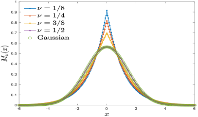
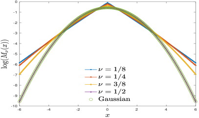
Refer to caption
Refer to caption
(a) Mainardi function for fractional diffusion, 0<ν<1/20𝜈120<\nu<1/2.
Refer to caption
Refer to caption
(b) Mainardi function for fractional wave propagation, 1/2<ν<112𝜈11/2<\nu<1.
Figure 9: The Mainardi function (left) and that in logarithm scale (right) for fractional diffusion equations and fractional wave equations.

The choice of threshold xλsubscript𝑥𝜆x_{\lambda} can be made by searching a point that matches the Laguerre-Gauss quadrature and the asymptotic leading term. For instance, we have found that xλ,μ=1.852subscript𝑥𝜆𝜇1.852x_{\lambda,\mu}=1.852 for ν=0.9𝜈0.9\nu=0.9, xλ,μ=1.41subscript𝑥𝜆𝜇1.41x_{\lambda,\mu}=1.41 for ν=0.95𝜈0.95\nu=0.95 and xλ,μ=1.087subscript𝑥𝜆𝜇1.087x_{\lambda,\mu}=1.087 for ν=0.99𝜈0.99\nu=0.99 can achieve a difference less than 107superscript10710^{-7} between the results produced by the Laguerre-Gauss quadrature and the asymptotic leading term.

To summarize, we use the following program to estimate the Mainardi function.

  • (1)

    When λ=12𝜆12\lambda=-\frac{1}{2} , we use the formula (1.3).

  • (2)

    When 12<λ<012𝜆0-\frac{1}{2}<\lambda<0, we use the formula (1.5).

  • (3)

    When 1<λ<121𝜆12-1<\lambda<-\frac{1}{2} and x<1cos(λπ)𝑥1𝜆𝜋x<-\frac{1}{\cos(\lambda\pi)}, we use the formula (1.6).

  • (4)

    When 1<λ<121𝜆12-1<\lambda<-\frac{1}{2} and 1cos(λπ)x<xλ1𝜆𝜋𝑥subscript𝑥𝜆-\frac{1}{\cos(\lambda\pi)}\leq x<x_{\lambda}, we use the formula (1.8).

  • (5)

    When 1<λ<121𝜆12-1<\lambda<-\frac{1}{2} and xxλ𝑥subscript𝑥𝜆x\geq x_{\lambda}, we use the asymptotic formula (1.9).

References

  • [1]

References

  • [1] E. Kjartansson, Constant Q-wave propagation and attenuation, J. Geophys. Res. 84.B9 (1979) 4737–4748.
  • [2] J. Virieux, P-SV wave propagation in heterogeneous media: Velocity-stress finite-difference method, Geophysics 51(4) (1986) 889–901.
  • [3] J. M. Carcione, F. Cavallini, F. Mainardi, A. Hanyga, Time-domain seismic modeling of constant-Q wave propagation using fractional derivatives, Pure Appl. Geophys. 159 (2002) 1714–1736.
  • [4] F. Mainardi, Fractional Calculus and Waves in Linear Viscoelasticity: An Introduction to Mathematical Models, World Scientific, Singapore, 2010. doi:10.1142/P614.
  • [5] F. Sun, J. Gao, N. Liu, The approximate constant Q and linearized reflection coefficients based on the generalized fractional wave equation, J. Acoust. Soc. Am. 145(1) (2019) 243–253.
  • [6] G. Xing, T. Zhu, A viscoelastic model for seismic attenuation using fractal mechanical networks, Geophys. J. Int. 224 (2021) 1658–1669.
  • [7] J. M. Carcione, Theory and modeling of constant-Q P- and S-waves using fractional time derivatives, Geophysics 74(1) (2009) 1787–1795.
  • [8] T. Zhu, J. M. Carcione, Theory and modelling of constant-Q P- and S-waves using fractional spatial derivatives, Geophys. J. Int. 3 (2014) 600.
  • [9] T. Zhu, J. M. Harris, B. Biondi, Q-compensated reverse-time migration, Geophysics 79(3) (2014) S77–S87.
  • [10] J. Sun, S. Fomel, T. Zhu, J. Hu, Q-compensated least-squares reverse time migration using low-rank one-step wave extrapolation, Geophysics 81(4) (2016) S271–S279.
  • [11] K. Shukla, J. M. Carcione, R. C. Pestana, P. Jaiswal, T. Ozdenvar, Modeling the wave propagation in viscoacoustic media: An efficient spectral approach in time and space domain, Comput. Geosci. 126 (2019) 31–40.
  • [12] K. Diethelm, An investigation of some nonclassical methods for the numerical approximation of Caputo-type fractional derivatives, Numer. Algor. 47(4) (2008) 361–390.
  • [13] Z. Wang, S. Vong, Compact difference schemes for the modified anomalous fractional sub-diffusion equation and the fractional diffusion-wave equation, J. Comput. Phys. 277 (2014) 1–15.
  • [14] H. Sun, X. Zhao, Z. Sun, The temporal second order difference schemes based on the interpolation approximation for the time multi-term fractional wave equation, J. Sci. Comput. 78 (2019) 467–498.
  • [15] J. Shen, C. Li, Z. Sun, An H2N2 interpolation for Caputo derivative with order in (1, 2) and its application to time-fractional wave equations in more than one space dimension, J. Sci. Comput. 83 (2020) 38.
  • [16] Y. Yang, Y. Chen, Y. Huang, H. Wei, Spectral collocation method for the time-fractional diffusion-wave equation and convergence analysis, Computers Math. Applic. 73(6) (2016) 1218–1232.
  • [17] V. R. Hosseni, E. Shivanian, W. Chen, Local radial point interpolation (MLRPI) method for solving time fractional diffusion-wave equation with damping, J. Comput. Phys. 312 (2016) 307–332.
  • [18] T. Zhu, Numerical simulation of seismic wave propagation in viscoelastic-anisotropic media using frequency-independent Q wave equation, Geophysics 82(4) (2017) WA1–WA10.
  • [19] W. Chen, S. Holm, Fractional Laplacian time-space models for linear and nonlinear lossy media exhibiting arbitrary frequency power-law dependency, J. Acoust. Soc. Am. 115(4) (2004) 1424–1430.
  • [20] T. Zhu, J. M. Harris, Modeling acoustic wave propagation in heterogeneous attenuating media using decoupled fractional Laplacians, Geophysics 79(3) (2014) T105–T116.
  • [21] J. M. Carcione, A generalization of the Fourier pseudospectral method, Geophysics 75(6) (2010) A53–A56.
  • [22] J. Yao, T. Zhu, F. Hussain, D. J. Kouri, Locally solving fractional Laplacian viscoacoustic wave equation using Hermite distributed approximating functional method, Geophysics 82(2) (2017) T59–T67.
  • [23] Q. Du, H. Han, J. Zhang, C. Zheng, Numerical solution of a two-dimensional nonlocal wave equation on unbounded domains, SIAM J. Sci. Comput. 40(3) (2018) A1430–A1445.
  • [24] C. Martinez, M. Sanz, L. Macro, Fractional powers of operators, J. Math. Soc. Japan 40(2) (1988) 331–347.
  • [25] J. E. Galé, P. J. Miana, P. R. Stinga, Extension problem and fractional operators: semigroups and wave equations, J. Evol. Equ. 13(2) (2013) 343–368.
  • [26] L. Yuan, O. P. Agrawal, A numerical scheme for dynamic systems containing fractional derivatives, J. Vib. Acoust. 124(2) (2002) 321–324.
  • [27] J. F. Lu, A. Hanyga, Wave field simulation for heterogeneous porous media with singular memory drag force, J. Comput. Phys. 208(2) (2005) 651–674.
  • [28] E. Blanc, G. Chiavassa, B. Lombard, Wave simulation in 2D heterogeneous transversely isotropic porous media with fractional attenuation: A Cartesian grid approach, J. Comput. Phys. 275 (2014) 118–142.
  • [29] J. Shen, T. Tang, L. Wang, Spectral Methods: Algorithms, Analysis and Applications, Springer-Verlag, Berlin, 2011.
  • [30] T. Tang, The Hermite spectral method for Gaussian-type functions, SIAM J. Sci. Comput. 14(3) (1993) 594–606.
  • [31] J. Shen, Stable and efficient spectral methods in unbounded domains using Laguerre functions, SIAM J. Numer. Anal. 38(4) (2000) 1113–1133.
  • [32] H. Ma, W. Sun, T. Tang, Hermite spectral methods with a time-dependent scaling for parabolic equations in unbounded domains, SIAM J. Numer. Anal. 43(1) (2006) 58–75.
  • [33] M. Xia, S. Shao, T. Chou, Efficient scaling and moving techniques for spectral methods in unbounded domains, accepted by SIAM. J. Sci. Comput., available at arXiv:2009.13170 (2020).
  • [34] B. Guo, L. Wang, Z. Wang, Generalized Laguerre interpolation and pseudospectral method for unbounded domains, SIAM J. Numer. Anal. 43(6) (2006) 2567–2589.
  • [35] H. Yoshida, Construction of higher order symplectic integrators, Phys. Lett. A 150 (1990) 262–268.
  • [36] A. Schmidt, L. Gaul, On a critique of a numerical scheme for the calculation of fractionally damped dynamical systems, Mech. Res. Commun. 33(1) (2006) 99–107.
  • [37] G. Szegö, Orthogonal Polynomials, American Mathematical Society, 1974.
  • [38] B. Fornberg, A practical guide to pseudospectral methods, Cambridge University Press, 1998.
  • [39] J. Burkardt, Generalized Gauss-Laguerre Quadrature Rules, https://people.sc.fsu.edu/similar-to\simjburkardt/f_src/gen_laguerre_rule/ (2010).
  • [40] Y. Luchko, Algorithms for evaluation of the Wright function for the real arguments’ values, Fract. Calc. Appl. Anal. 11(1) (2008) 57–75.