Fourth Painlevé Equation and $\mathcal{PT}$-Symmetric Hamiltonians

Abstract

This paper is an addendum to earlier papers R1 ; R2 in which it was shown that the unstable separatrix solutions for Painlevé I and II are determined by $\mathcal{PT}$-symmetric Hamiltonians. In this paper unstable separatrix solutions of the fourth Painlevé transcendent are studied numerically and analytically. For a fixed initial value, say $y(0)=1$, a discrete set of initial slopes $y^{\prime}(0)=b_{n}$ give rise to separatrix solutions. Similarly, for a fixed initial slope, say $y^{\prime}(0)=0$, a discrete set of initial values $y(0)=c_{n}$ give rise to separatrix solutions. For Painlevé IV the large-$n$ asymptotic behavior of $b_{n}$ is $b_{n}\sim B_{\rm IV}n^{3/4}$ and that of $c_{n}$ is $c_{n}\sim C_{\rm IV}n^{1/2}$. The constants $B_{\rm IV}$ and $C_{\rm IV}$ are determined both numerically and analytically. The analytical values of these constants are found by reducing the nonlinear Painlevé IV equation to the linear eigenvalue equation for the sextic $\mathcal{PT}$-symmetric Hamiltonian $H={\textstyle{\frac{1}{2}}}p^{2}+{\textstyle{\frac{1}{8}}}x^{6}$.

I Introduction

The six Painlevé transcendents satisfy nonlinear second-order differential equations having the property that their movable (spontaneous) singularities are poles (and not branch points or essential singularities). Many papers have been published on these equations (see, for example, References 1-8 in R2 for background information and References 9-16 in R2 for applications in mathematical physics). This paper considers the fourth Painlevé transcendent, referred to here as P-IV. There are many recent studies of this equation; see, for example, Refs. R3 ; R4 ; R5 ; R6 .

The initial-value problem for the P-IV differential equation examined here is

$$y(t)y^{\prime\prime}(t)={\textstyle{\frac{1}{2}}}[y^{\prime}(t)]^{2}+2t^{2}[y(t)]^{2}+4t[y(t)]^{3}+{\textstyle{\frac{3}{2}}}[y(t)]^{4},\quad y(0)=c,~{}y^{\prime}(0)=b.$$ (1)

(For simplicity we have set the two arbitrary constants in P-IV, one of which is a trivial additive constant, to 0.) There have been many asymptotic studies of the Painlevé transcendents, but here we present a simple numerical and asymptotic analysis that has not appeared in the literature. This analysis concerns the initial conditions that give rise to special unstable separatrix solutions of P-IV. The asymptotic analysis here extends our earlier work on nonlinear differential-equation eigenvalue problems in R2 ; R7 ; R8 .

The idea, originally proposed in Ref. R6 , is that a nonlinear differential equation may have a discrete set of critical initial conditions that give rise to unstable separatrix solutions. These discrete initial conditions can be thought of as eigenvalues and the separatrices stemming from these initial conditions can be viewed as corresponding eigenfunctions. The objective in Ref. R6 is to find the large-$n$ (semiclassical) asymptotic behavior of t he $n$th eigenvalue. The analytical approach is to reduce the nonlinear differential-equation problem to a linear problem that could be solved to determine the asymptotic behavior of the eigenvalues as $n\to\infty$.

A toy model used in Ref. R6 to explore the properties of nonlinear eigenvalue problems is the first-order differential-equation problem

$$y^{\prime}(t)=\cos[\pi t\,y(t)],\quad y(0)=a.$$ (2)

The solutions to this initial-value problem exhibit $n$ maxima before vanishing like $1/t$ as $t\to\infty$. As the initial condition $a$ increases past critical values $a_{n}$, the number of maxima of $y(t)$ jumps from $n$ to $n+1$. At $a_{n}$ the solution $y(t)$ is an unstable separatrix: If $y(0)$ is slightly below $a_{n}$, $y(x)$ merges with a bundle of stable solutions all having $n$ maxima and when $y(0)$ is slightly above $a_{n}$, $y(x)$ merges with a bundle of stable solutions all having $n+1$ maxima. We seek the asymptotic behavior of $a_{n}$ for large $n$, which is the analog of a high-energy semiclassical approximation in quantum mechanics. In Ref. R6 it is shown that for large $n$ the nonlinear differential equation (2) reduces to a linear difference equation for a one-dimensional random walk. The difference equation is solved exactly, and it is shown that

$$a_{n}\sim 2^{5/6}\sqrt{n}\quad(n\to\infty).$$ (3)

Kerr subsequently found an alternative solution to this asymptotics problem and verified (3) R9 .

The nonlinear eigenvalue problem described above is similar in many respects to the linear eigenvalue problem for the time-independent Schrödinger equation. For a potential $V(x)$ that rises as $x\to\pm\infty$, the eigenfunctions $\psi(x)$ of the Schrödinger eigenvalue problem

$$-\psi^{\prime\prime}(x)+V(x)\psi(x)=E\psi(x),\quad\psi(\pm\infty)=0,$$ (4)

are unstable with respect to small changes in the eigenvalue $E$; that is, if $E$ is increased or decreased slightly, $\psi(x)$ abruptly violates the boundary conditions (is not square integrable). Also, like the eigenfunctions (separatrix curves) of (2), the $n$th eigenfunction $\psi_{n}(x)$ has $n$ oscillations in the classically allowed region before decreasing monotonically to $0$ in the classically forbidden region.

This paper considers two eigenvalue problems for P-IV. First, we find the large-$n$ behavior of the positive eigenvalues $b_{n}$ for the initial condition $y(0)=1,\,y^{\prime}(0)=b_{n}$ and also the large-$n$ behavior of the negative eigenvalues $c_{n}$ for the initial condition $y(0)=c_{n},\,y^{\prime}(0)=0$. We show that

$$b_{n}\sim B_{\rm IV}n^{3/4}\quad{\rm and}\quad c_{n}\sim C_{\rm IV}n^{1/2}.$$ (5)

In Sec. II we compute the constants $B_{\rm IV}$ and $C_{\rm IV}$ numerically and in Sec. III we find them analytically by reducing the large-eigenvalue problem to the linear time-independent Schrödinger equation for the sextic $\mathcal{PT}$-symmetric Hamiltonian $H={\textstyle{\frac{1}{2}}}p^{2}+x^{6}$. Section IV gives brief concluding remarks.

II Numerical analysis of the fourth Painlevé transcendent

There are three possible asymptotic behaviors of the solutions to the P-IV equation as $t\to-\infty$; $y(t)$ can approach the straight lines $y=-2t$, $y=-2t/3$, or $y=0$. An elementary asymptotic analysis shows that if $y(t)$ approaches $y=-2t/3$, the solution oscillates stably about this line with slowly decreasing amplitude R10 . However, while $y=-2t$ and $y=0$ are possible asymptotic behaviors, these behaviors are unstable and nearby solutions veer away from them. Here we consider the eigenfunction solutions to P-IV that approach $y=-2t$ as $t\to-\infty$. These separatrix solutions resemble quantum-mechanical eigenfunctions because they have $n$ oscillations before exhibiting this asymptotic behavior. Because the P-IV equation is nonlinear these oscillations are unbounded; the $n$th eigenfunction passes through $[n/2]$ simple poles before smoothly approaching $y=-2t$ ($[n/2]$ is the greatest integer in $\leq n/2$).

We consider two different eigenvalue problems for P-IV that are related to the instability of the asymptotic behavior $y=-2t$: (i) We fix the initial value $y(0)=1$ and seek the discrete values of the initial slopes $y^{\prime}(0)=b$ that give solutions approaching $-2t$, and (ii) we fix the initial slope $y^{\prime}(0)=0$ and seek the discrete initial values of $y(0)=c$ for which $y(t)$ approaches $-2t$.

II.1 Initial-slope eigenvalues for Painlevé IV

Let us examine the solutions to the initial-value problem for P-IV in (1) for $t<0$. As in Ref. R2 , we find these solutions numerically by using Runge-Kutta to integrate down the negative-real axis. When we approach a simple pole, we integrate along a semicircle in the complex-$t$ plane around the pole and continue integrating down the negative axis. We choose the initial value $y(0)=1$ and allow the initial slope $y^{\prime}(0)=b$ to have increasingly positive values. (We only present results for positive initial slope; the P-IV equation is symmetric under $t\to-t$ and also under $y\to-y$.) Numerical study shows that the choice of $y(0)$ is not crucial if $y(0)\neq 0$; for any $y(0)$ the large-$n$ behavior of the initial-slope eigenvalues $b_{n}$ is the same.

Above the first eigenvalue $b_{1}=3.15837325$ there is a continuous interval of $b$ for which $y(t)$ has an infinite sequence of simple poles (Fig. 1, left panel). When $b$ increases above the next eigenvalue $b_{2}=6.18498704$, the character of the solutions changes abruptly and after $y(t)$ passes through a finite number of simple poles it begins to oscillate stably about $-2t/3$ (Fig. 1, right panel). When $b$ exceeds the third eigenvalue $b_{3}=8.79172082$, the solutions again pass through an infinite sequence of poles (Fig. 2, left panel). When $b$ increases above $b_{4}=11.1720921$, the solutions again oscillate stably about $-2t/3$ (Fig. 2, right panel). Numerical study verifies that there is an infinite sequence of eigenvalues at which the solutions to P-IV alternate between infinite sequences of simple poles and stable oscillation about $-2t/3$.

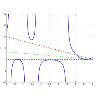
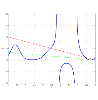
Figure 1: [Color online] Behavior of solutions $y(t)$ to the P-IV equation (1) for initial conditions $y(0)=1$ and $b=y^{\prime}(0)$. Left panel: $b=5.18498704$, which lies between the eigenvalues $b_{1}=3.15837325$ and $b_{2}=6.18498704$. Right panel: $b=7.18498704$, which lies between $b_{2}=6.18498704$ and $b_{3}=8.79172082$. The upper dashed line (red) is $y=-2t$, which is unstable and the lower dashed line (stable) is $y=-2t/3$. In the left panel $y(t)$ has an infinite sequence of simple poles but in the right panel the poles abruptly end and solution then oscillates stably about $-2t/3$.

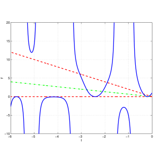
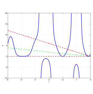
Figure 2: [Color online] Solutions to the P-IV equation (1) for $y(0)=0$ and $b=y^{\prime}(0)$. Left panel: $b=10.1720921$, which lies between the eigenvalues $b_{3}=8.79172082$ and $b_{4}=11.1720921$. Right panel: $b=12.1720921$, which lies between the eigenvalues $b_{4}=11.1720921$ and $b_{5}=13.3990049$.

When $y^{\prime}(0)$ is an eigenvalue the solutions exhibit a completely different and unstable behavior from those in Figs. 1 and 2. These solutions pass through a finite number of simple poles (like the oscillations of quantum-mechanical eigenfunctions in a classically allowed region) and then have a turning-point-like transition in which the poles cease and $y(t)$ exponentially approaches the line $-2t$. The solutions arising from the first and second eigenvalues $b_{1}$ and $b_{2}$ are shown in Fig. 3, those arising from $b_{3}$ and $b_{4}$ are shown in Fig. 4, and those arising from $b_{11}$ and $b_{12}$ are shown in Fig. 5. The critical values $b_{n}$ are analogous to eigenvalues because they generate unstable separatrix solutions; if $y^{\prime}(0)$ changes by a small amount above or below a critical value, the character of the solutions changes abruptly and the solutions exhibit the two possible generic behaviors shown in Figs. 1 and 2.

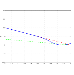
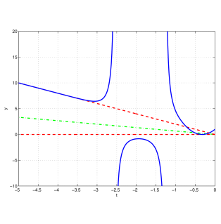
Figure 3: [Color online] First two separatrix (eigenfunction) solutions of P-IV with initial condition $y(0)=0$. Left panel: $y^{\prime}(0)=b_{1}=3.15837325$; right panel: $y^{\prime}(0)=b_{2}=6.18498704$. The dashed lines are $y=-2t$ and $y=-2t/3$.

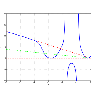
Figure 4: [Color online] Third and fourth eigenfunctions of P-IV with initial condition $y(0)=0$. Left panel: $y^{\prime}(0)=b_{3}=8.79172082$; right panel: $y^{\prime}(0)=b_{4}=11.1720921$.

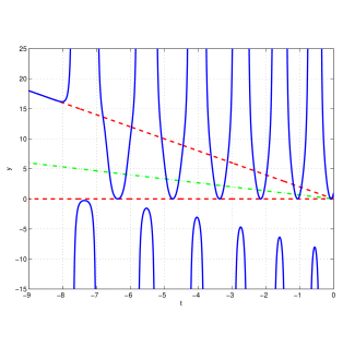
Figure 5: [Color online] Eleventh and twelth eigenfunctions of P-IV with initial condition $y(0)=0$. Left panel: $y^{\prime}(0)=b_{11}=24.9911479$; right panel: $y^{\prime}(0)=b_{12}=26.7370929$. As $n$ increases, the eigenfunctions pass through more and more simple poles before exhibiting a turning-point transition and approaching the limiting curve $-2t$ exponentially rapidly. This behavior is analogous to that of the eigenfunctions of a time-independent Schrödinger equation for a particle in a potential well; the higher-energy eigenfunctions exhibit more and more oscillations in the classically allowed region before entering the classically forbidden region, where they decay to zero.

As in Ref. R2 for P-I and P-II, we have performed a numerical asymptotic study of the critical values $b_{n}$ for $n\gg 1$ by using Richardson extrapolation R10 . [In this paper we have taken $y(0)=1$ but we find that if $y(0)$ is held fixed, the large-$n$ behavior of the initial slope $b_{n}$ is insensitive to the choice of $y(0)$.] By applying fifth-order Richardson extrapolation to the first twelve eigenvalues, we find the value of $B_{\rm IV}$ accurate to one part in seven decimal places:

$$B_{\rm IV}=4.25684{\underline{3}}.$$ (6)

II.2 Initial-value eigenvalues for Painlevé IV

If we fix the initial slope at $y^{\prime}(0)=0$ and allow the initial value $y(0)=c$ to become increasingly negative, we find a sequence of negative eigenvalues $c_{n}$ for which the solutions behave like the separatrix (eigenfunction) solutions in Figs. 3–5. The first two eigenfunctions are plotted in Fig. 6, the next two in Fig. 7, and the eleventh and twelth in Fig. 8.

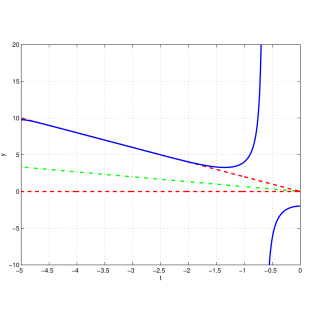
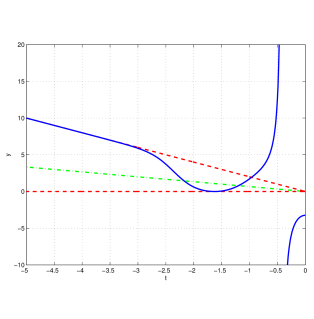
Figure 6: [Color online] First two separatrix solutions (eigenfunctions) of Painlevé IV with fixed initial slope $y^{\prime}(0)=0$. Left panel: $y(0)=c_{1}=-1.98740393$; right panel: $y(0)=c_{2}=-3.23535569$. The dashed curves are $y=-2t$ and $t=-2t/3$.

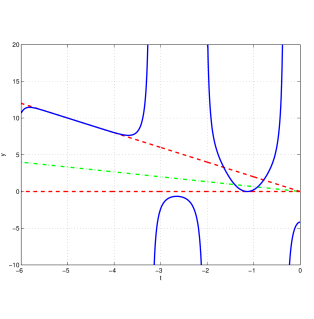
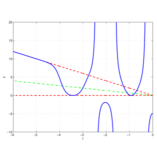
Figure 7: [Color online] Third and fourth eigenfunctions of Painlevé IV with initial slope $y^{\prime}(0)=0$. Left panel: $y(0)=c_{3}=-4.1616081$; right panel: $y(0)=c_{4}=-4.91908695$.

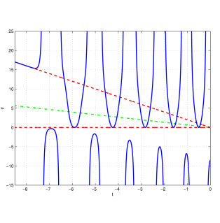
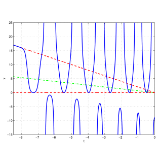
Figure 8: [Color online] Eleventh and twelth eigenfunctions of Painlevé IV with initial slope $y^{\prime}(0)=0$. Left panel: $y(0)=c_{11}=-8.51211189$; right panel: $y(0)=c_{12}=-8.90805963$.

Applying fourth-order Richardson extrapolation to the first 15 eigenvalues, we find that for large $n$ the sequence of initial-value eigenvalues $c_{n}$ is asymptotic to $C_{\rm IV}n^{1/2}$, where

$$C_{\rm IV}=-2.62658{\underline{7}}.$$ (7)

III Asymptotic determination of $B_{\rm VI}$ and $C_{\rm IV}$

In this section we present an asymptotic analysis that yields analytic formulas for $B_{\rm IV}$ and $C_{\rm IV}$ in (6) and (7). To begin, we rewrite the P-IV equation (1) as

$$2[y(t)]^{3/2}\left[\sqrt{y(t)}\right]^{\prime\prime}=2t^{2}[y(t)]^{2}+4t[y(t)]^{3}+\frac{3}{2}[y(t)]^{4}.$$

This suggests the substitution $u(t)=\sqrt{y(t)}$, which gives the equation

$$u^{\prime\prime}(t)=t^{2}u(t)+2t[u(t)]^{3}+\frac{3}{4}[u(t)]^{5}.$$

Following Ref. R2 we multiply by $u^{\prime}(t)$ and integrate from $t=0$ to $t=x$:

$$H\equiv-{\textstyle{\frac{1}{2}}}[u^{\prime}(x)]^{2}+{\textstyle{\frac{1}{8}}}[u(x)]^{6}=-{\textstyle{\frac{1}{2}}}[u^{\prime}(0)]^{2}+{\textstyle{\frac{1}{8}}}[u(0)]^{6}-I(x),$$ (8)

where $I(x)=\int_{0}^{x}dt\left(t^{2}u(t)u^{\prime}(t)+2t[u(t)]^{3}u^{\prime}(t)\right)$. The path of $t$ integration used here is like that used to compute $y(t)$ numerically in Sec. II; the path follows a straight line until it approaches a pole, at which point it makes a semicircular detour in the complex-$t$ plane to avoid the pole.

If we evaluate $H(x)$ on the imaginary-$t$ axis we obtain the Hamiltonian

$$\hat{H}={\textstyle{\frac{1}{2}}}{\hat{p}}^{2}+{\textstyle{\frac{1}{8}}}{\hat{x}}^{6}.$$ (9)

This Hamiltonian can be interpreted in two possible ways, either as a Hermitian Hamiltonian for which the eigenfunctions vanish as $x\to\pm\infty$ or as a $\mathcal{PT}$-symmetric Hamiltonian for which the eigenfunctions vanish as $|x|\to\infty$ with ${\rm arg}\,x=-{\textstyle{\frac{1}{4}}}\pi$ and $-{\textstyle{\frac{3}{4}}}\pi$. To see which quantization scheme is correct we calculate $I(x)$ numerically (see Fig. 9).

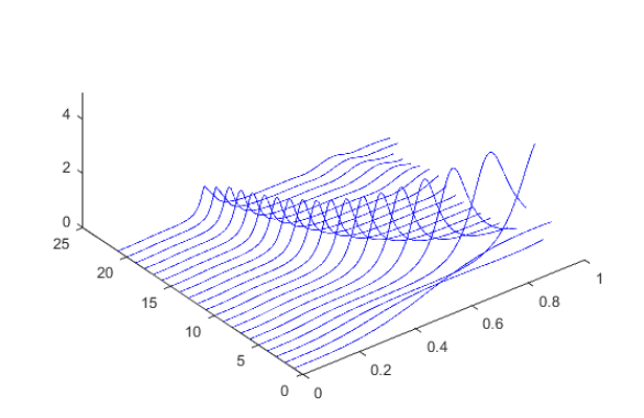
Figure 9: [Color online] Numerical evidence that $I(x)$ is small for fixed $x$ as $n\to\infty$.

We find numerically that on the lines ${\rm arg}\,x=-{\textstyle{\frac{1}{4}}}\pi$ and $-{\textstyle{\frac{3}{4}}}\pi$ the function $I(x)$ and becomes small compared with $H$ as $n\to\infty$ for fixed $x$. Thus, for an eigenfunction of P-IV we can interpret $H$ as a time-independent quantum-mechanical Hamiltonian. We conclude that the large-$n$ (semiclassical) behavior of the P-IV eigenvalues can be determined by solving the linear quantum-mechanical eigenvalue problem $\hat{H}\psi=E\psi$, where $\hat{H}={\textstyle{\frac{1}{2}}}{\hat{p}}^{2}+\frac{1}{8}{\hat{x}}^{6}$. The large eigenvalues of this Hamiltonian can be found by using the complex WKB techniques discussed in detail in Ref. R11 . For the general class of $\mathcal{PT}$-symmetric Hamiltonians $\hat{H}={\textstyle{\frac{1}{2}}}\hat{p}^{2}+g\hat{x}^{2}\left(i\hat{x}\right)^{\varepsilon}$ $(\varepsilon\geq 0)$, the WKB approximation to the $n$th eigenvalue $(n\gg 1)$ is given by

$$E_{n}\sim\frac{1}{2}(2g)^{2/(4+\varepsilon)}\left[\frac{\Gamma\left(\frac{3}{2}+\frac{1}{\varepsilon+2}\right)\sqrt{\pi}\,n}{\sin\left(\frac{\pi}{\varepsilon+2}\right)\Gamma\left(1+\frac{1}{\varepsilon+2}\right)}\right]^{(2\varepsilon+4)/(\varepsilon+4)}.$$ (10)

Thus, for $H$ in (9) we take $g=1/8$ and $\varepsilon=4$ and obtain the asymptotic behavior

$$E_{n}\sim\left[\sqrt{\pi}\Gamma\left(\textstyle{\frac{5}{3}}\right)n/\Gamma\left(\textstyle{\frac{7}{6}}\right)\right]^{3/2}\quad(n\to\infty).$$ (11)

Since $\hat{H}$ in (9) is time independent, we can evaluate $H$ in (8) for fixed $y(0)$ and large $y^{\prime}(0)=b_{n}$ and obtain the result that

$$b_{n}\sim 4\sqrt{E_{n}/2}=B_{\rm IV}n^{3/4}\quad(n\to\infty),$$ (12)

which verifies (5). We then read off the analytic value of the constant $B_{\rm IV}$:

$$B_{\rm IV}=2^{3/2}\left[\sqrt{\pi}\Gamma\left(\textstyle{\frac{5}{3}}\right)/\Gamma\left(\textstyle{\frac{7}{6}}\right)\right]^{3/4},$$ (13)

which agrees with the numerical result in (6). Also, if we take the initial slope $y^{\prime}(0)$ to vanish and take the initial condition $y(0)=c_{n}$ to be large, we obtain an analytic expression for $C_{\rm IV}$,

$$C_{\rm IV}=-2\left[\sqrt{\pi}\Gamma\left(\textstyle{\frac{5}{3}}\right)/\Gamma\left(\textstyle{\frac{7}{6}}\right)\right]^{1/2},$$ (14)

which agrees with the numerical result in (7).

IV Concluding remarks

In this paper we have shown that the fourth Painlevé equation P-IV exhibits instabilities that are associated with separatrix solutions. The initial conditions that give rise to these separatrix solutions are eigenvalues. We have calculated the semiclassical (large-eigenvalue) behavior of the eigenvalues in two ways, first by using numerical techniques and then by using asymptotic methods to reduce the initial-value problems for the nonlinear P-IV equation (1) to the linear eigenvalue problem associated with the time-independent Schrödinger equation for the $\mathcal{PT}$-symmetric $x^{6}$ potential. The agreement between these two approaches is exact.

The obvious continuation of this work is to examine the three remaining Painlevé equations, P-III, P-V, and P-VI, to see if there are instabilities, separatrices, and eigenvalues for these equations as well. It is quite surprising that P-I, P-II, and P-IV are associated with the $\mathcal{PT}$-symmetric $x^{2}(ix)^{\varepsilon}$ for the values $\varepsilon=1$, 2, and 4 and it will be interesting to see if these more complicated Painlevé equations have associated values of $\varepsilon$ as well.

- (1) C. M. Bender, A. Fring, and J. Komijani, J. Phys. A: Math. Theor. 47, 235204 (2014).
- (2) C. M. Bender and J. Komijani, J. Phys. A: Math. Theor. 48, 475202 (2015).
- (3) J. Reeger and B. Fornberg, Stud. App. Math. 130, 108 (2012).
- (4) J. Reeger and B. Fornberg, Physica D 280-281, 1 (2014).
- (5) D. J. Fernández and J. L. González, Ann. Phys. 359, 213 (2015).
- (6) J. Schiff and M. Twiton, J. Phys. A: Math. Theor. 52, 145201 (2019) and arXiv:1905.12125.
- (7) C. M. Bender, J. Komijani, and Q-h. Wang, in Resurgence, Physics and Numbers, ed. by F. Fauvet, D. Manchon, S. Marmi, and D. Sauzin, CRM Series, Ennio De Georgi 20, 67-89 (2017).
- (8) C. M. Bender, J. Komijani, and Q-h. Wang, J. Phys. A: Math. Theor. 52, 315202 (2019).
- (9) O. S. Kerr, J. Phys. A: Math. Theor. 47, 368001 (2014).
- (10) C. M. Bender and S. A. Orszag, Advanced Mathematical Methods for Scientists and Engineers (McGraw Hill, New York, 1978).
- (11) C. M. Bender and S. Boettcher, Phys. Rev. Lett. 80, 5243 (1988).