A posteriori error analysis for a distributed optimal control problem governed by the von Kármán equations

Abstract

This article discusses numerical analysis of the distributed optimal control problem governed by the von Kármán equations defined on a polygonal domain in $\mathbb{R}^{2}$. The state and adjoint variables are discretised using the nonconforming Morley finite element method and the control is discretized using piecewise constant functions. A priori and a posteriori error estimates are derived for the state, adjoint and control variables. The a posteriori error estimates are shown to be efficient. Numerical results that confirm the theoretical estimates are presented.

Keywords: von Kármán equations, distributed control, plate bending, non-linear, nonconforming, Morley FEM, a priori, a posteriori, error estimates

1 Introduction

Problem formulation

Let $\Omega\subset\mathbb{R}^{2}$ be a polygonal domain and $\nu$ denotes the outward normal vector to the boundary $\partial\Omega$ of $\Omega$. This paper considers the distributed control problem governed by the von Kármán equations stated below:

$$\min_{u\in U_{ad}}\mathcal{J}(\Psi,u)\,\,\,\textrm{ subject to }$$ (1.1a)

$$\Delta^{2}\psi_{1}=[\psi_{1},\psi_{2}]+f+{\mathcal{C}}u,\,\,\Delta^{2}\psi_{2}=-\frac{1}{2}[\psi_{1},\psi_{1}]\mbox{ in }\Omega,$$ (1.1b)

$$\psi_{1}=0,\,\frac{\partial\psi_{1}}{\partial\nu}=0\text{ and }\psi_{2}=0,\,\frac{\partial\psi_{2}}{\partial\nu}=0\text{ on }\partial\Omega.$$ (1.1c)

Here the cost functional $\displaystyle\mathcal{J}(\Psi,u):=\frac{1}{2}|\!|\!|\Psi-\Psi_{d}|\!|\!|_{\boldsymbol{L}^{2}(\Omega)}^{2}+\frac{\alpha}{2}\|{u}\|_{L^{2}(\omega)}^{2}\>{\rm\,dx}$, the state variable $\Psi:=(\psi_{1},\psi_{2})$, where $\psi_{1}$ and $\psi_{2}$ correspond to the displacement and Airy-stress, $\Psi_{d}:={(\psi_{d,1},\psi_{d,2})}\in\boldsymbol{L}^{2}(\Omega):=L^{2}(\Omega)\times L^{2}(\Omega)$ is the prescribed desired state for $\Psi$, $|\!|\!|\Psi-\Psi_{d}|\!|\!|_{\boldsymbol{L}^{2}(\Omega)}^{2}:=\sum_{i=1}^{2}\|\psi_{i}-\psi_{d,i}\|_{L^{2}(\Omega)}^{2}$, $\alpha>0$ is a fixed regularization parameter, $U_{ad}\subset L^{2}(\omega)$, $\omega\subset\Omega$ is a non-empty, closed, convex and bounded set of admissible controls defined by

$$U_{ad}=\{u\in L^{2}(\omega):u_{a}\leq u(x)\leq u_{b}\;\mbox{ for almost every }x\mbox{ in }\omega\},$$

$u_{a}\leq u_{b}\in{\mathbb{R}}$ are given, $\Delta^{2}$ denotes the fourth-order biharmonic operator, the von Kármán bracket $[\eta,\chi]:=\eta_{xx}\chi_{yy}+\eta_{yy}\chi_{xx}-2\eta_{xy}\chi_{xy}={\rm cof}(D^{2}\eta):D^{2}\chi$ with the co-factor matrix ${\rm cof}(D^{2}\eta)$ of $D^{2}\eta$, $f\in L^{2}(\Omega)$, and ${\mathcal{C}}\in{\mathcal{L}}(L^{2}(\omega),L^{2}(\Omega))$ is the extension operator defined by ${\mathcal{C}}u(x)=u(x)\mbox{ if }x\in\omega\mbox{ and }{\mathcal{C}}u(x)=0\mbox{ if }x\not\in\omega.$

Motivation

The optimal control problem governed by the von Kármán equations (1.1a)-(1.1c) is analysed in [31] for $C^{1}$ conforming finite elements. In [19], a priori error estimates are derived under minimal regularity assumptions on the exact solution where the state and adjoint variables are discretised using Morley finite element methods (FEMs). The discrete trilinear form in the weak formulation [19] is derived after an integration by parts. In this article, a simplified form of the trilinear form that involves the von Kármán bracket itself is considered. This choice of the trilinear form [11] is appropriate for both reliable and efficient a posteriori estimates. To the best of our knowledge, there are no results in literature that discuss a posteriori error analysis for the approximation of regular solutions of optimal control problems governed by von Kármán equations. Recently, a posteriori error analysis for the optimal control problem governed by second-order stationary Navier-Stokes equations is studied in [1] with conforming finite element method under smallness assumption on the data. The trilinear form in [1] vanishes whenever the second and third variables are equal, and satisfies the anti-symmetric property with respect to the second and third variables and this aids the a posteriori error analysis. This paper discusses approximation of regular solutions for fourth-order semi-linear problems without any smallness assumption on the data. Moreover, the trilinear form for von Kármán equations does not satisfy the properties stated above and hence leads to additional challenges in the analysis.

The von Kármán equations [21] that describes the bending of very thin elastic plates offers challenges in its numerical approximation; mainly due to its nonlinearity and higher order nature; we refer to [21, 27, 3, 2, 4, 5] and the references therein for the existence of solutions, regularity and bifurcation phenomena of the von Kármán equations. The numerical analysis of von Kármán equations has been studied using conforming FEMs in [9, 29], nonconforming Morley FEM in [30, 12], mixed FEMs in [32, 17], discontinuous Galerkin methods and $C^{0}$ interior penalty methods in [6, 11].

Nonconforming Morley FEM based on piecewise quadratic polynomials in a triangle is more elegant, attractive and simpler for fourth-order problems. However, the convergence analysis offers a lot of novel challenges in the context of control problems governed by semilinear problems with trilinear nonlinearity since the discrete space $V_{\text{M}}$ is not a subspace of $H^{2}_{0}(\Omega)$. The adjoint variable in the control problem satisfies a fourth-order linear problem with lower-order terms and its a priori and a posteriori analysis with Morley FEM offers additional difficulties.

The regularity results of von Kármán equations in [5] extends to the regularity of the state and adjoint variables of the control problem [31] and ensures that the optimal state and adjoint variables belong to $H^{2}_{0}(\Omega)\cap H^{2+\gamma}(\Omega)$, where $\gamma\in(\frac{1}{2},1]$, referred to as the index of elliptic regularity, is determined by the interior angles of $\Omega$. Note that when $\Omega$ is convex, $\gamma=1$.

Contributions

In continuous formulation (see (2.1)) and the conforming FEM [31], the trilinear form $b(\bullet,\bullet,\bullet)$ is symmetric with respect to all the three variables; that makes the analysis simpler to a certain extent. However, for fourth-order systems, nonconforming Morley FEM is attractive and is a method of choice [12] and this motivated the a priori analysis for the optimal control problem in [19]. The expression for the discrete trilinear form $\displaystyle b_{\text{NC}}(\bullet,\bullet,\bullet)$ in [19] defined as $\frac{1}{2}\sum_{T\in\mathcal{T}}\int_{T}{\rm{cof}}(D^{2}\eta_{\text{M}})D\chi_{\text{M}}\cdot D\varphi_{\text{M}}{\rm\,dx}$ for all Morley functions $\eta_{\text{M}},\chi_{\text{M}}\;\text{and}\;\varphi_{\text{M}}$ is obtained after an integration by parts, where $\mathcal{T}$ denotes the triangulation of $\Omega$. This form is symmetric with respect to the second and third variables. Though this choice of trilinear form leads to optimal order error estimates for the optimal control problem (1.1a)-(1.1c), it leads to terms that involve averages in the reliability analysis of the state equations (as in the case of Navier-Stokes equation considered in [12]). The efficiency estimates are unclear in this context. To overcome this, a more natural trilinear form $\displaystyle b_{\text{NC}}(\eta_{\text{M}},\chi_{\text{M}},\varphi_{\text{M}})=-\frac{1}{2}\sum_{T\in\mathcal{T}}\int_{T}[\eta_{\text{M}},\chi_{\text{M}}]\varphi_{\text{M}}{\rm\,dx}$ that is symmetric with respect to the first and second variables is chosen in this article. The a priori and a posteriori analysis for the state equations are discussed in [12, 13]. The a posteriori analysis for the fully discrete optimal control problem governed by von Kármán equations addressed in this article is novel and involves additional difficulties. For instance, the adjoint system in this case involves lower-order terms with leading biharmonic operators. A posteriori analysis for biharmonic operator with lower-order terms is a problem of independent interest.

Thus the contributions of this article can be summarized as follows.

• For a formulation that is different from that in [19], optimal order a priori error estimates in energy norm when state and adjoint variables are approximated by Morley FEM and linear order of convergence for control variable in $L^{2}$ norm when control is approximated using piece-wise constants are outlined.

• Reliable and efficient a posteriori error estimates that drive the adaptive refinement for the optimal state and adjoint variables in the energy norm and control variable in the $L^{2}$ norm are developed. The approach followed in this paper provides a strategy for the nonconforming FEM analysis of optimal control problems governed by higher-order semi-linear problems.

• Several auxiliary results that are derived will be of interest in other applications - for example, optimal control problems governed by Navier-Stokes problems in the stream-vorticity formulation.

• The paper illustrates results of computational experiments that validate both theoretical a priori and a posteriori estimates for the optimal control problem under consideration.

Organisation

The remaining parts of this paper are organised as follows. Section 2 presents the weak and the nonconforming finite element formulations for (1.1a)-(1.1c). The state and adjoint variables are discretised using Morley finite elements and the control variable is discretised using piecewise constant functions. Section 2.3 deals some preliminaries related to Morley FEM. The boundedness properties of the discrete bilinear and trilinear forms that are crucial for the error analysis are discussed in this section. A priori error estimates for the state, adjoint and control variables under minimal regularity assumptions on the exact solution are stated in Section 3. Note that the analysis differs from [19] due to a different trilinear form. Section 4 develops reliable a posteriori estimates for the state, adjoint and control variables of the optimal control problem. Section 5 establishes efficiency results for the optimal control problem. Results of numerical experiments that validate theoretical estimates are presented in Section 6. Finally, details of proofs of some results stated in Section 3 are derived in the Appendix.

Notations

Throughout the paper, standard notations on Lebesgue and Sobolev spaces and their norms are employed. The standard semi-norm and norm on $H^{s}(\Omega)$ (resp. $W^{s,p}(\Omega)$) for $s>0$ and $1\leq p\leq\infty$ are denoted by $|\cdot|_{s}$ and $\|\cdot\|_{s}$ (resp. $|\cdot|_{s,p}$ and $\|\cdot\|_{s,p}$ ) and norm in $L^{\infty}(\Omega)$ is denoted by $\|\cdot\|_{0,\infty}$. The norm in $H^{-s}(\Omega)$ is denoted by $\|\cdot\|_{-s}$. The standard $L^{2}$ inner product and norm are denoted by $(\cdot,\cdot)$ and $\|\cdot\|.$ The notation $\|\cdot\|$ is also used to denote the operator norm and should be understood from the context. The notation ${\boldsymbol{H}}^{s}(\Omega)$ (resp. ${\boldsymbol{L}}^{p}(\Omega)$) is used to denote the product space $H^{s}(\Omega)\times H^{s}(\Omega)$ (resp. $L^{p}(\Omega)\times L^{p}(\Omega)$). For all $\Phi=(\varphi_{1},\varphi_{2})\in{\boldsymbol{H}}^{s}(\Omega)\;(\text{resp. }{\boldsymbol{L}}^{2}(\Omega))$, the product space is equipped with the norm $|\!|\!|{\Phi}|\!|\!|_{s}:=(\|\varphi_{1}\|_{s}^{2}+\|\varphi_{2}\|_{s}^{2})^{1/2}\;(\text{ resp. }|\!|\!|{\Phi}|\!|\!|:=(\|\varphi_{1}\|^{2}+\|\varphi_{2}\|^{2})^{1/2}).\;$ The notation $a\lesssim b$ (resp. $a\gtrsim b$) means there exists a generic mesh independent constant $C$ such that $a\leq Cb$ (resp. $a\geq Cb$). The positive constants $C$ appearing in the inequalities denote generic constants which do not depend on the mesh-size.

2 Weak and Finite Element Formulations

In this section, the weak and Morley FEM formulations for (1.1a)-(1.1c) and some auxiliary results are presented.

2.1 Weak Formulation

Let $V:=H^{2}_{0}(\Omega)$, $\text{\bf V}=V\times V$, the bilinear (resp. trilinear) form $a(\bullet,\bullet):V\times V\rightarrow\mathbb{R}$ (resp. $b(\bullet,\bullet,\bullet):V\times V\times V\rightarrow\mathbb{R}$) be defined by

$$a(\varphi_{1},\varphi_{2}):=\int_{\Omega}D^{2}\varphi_{1}:D^{2}\varphi_{2}\;{\rm\,dx}\;\;(\mbox{resp. }b(\varphi_{1},\varphi_{2},\varphi_{3}):=-\frac{1}{2}\int_{\Omega}[\varphi_{1},\varphi_{2}]\varphi_{3}\;{\rm\,dx}).$$

For all $\varphi_{1},\varphi_{2},\varphi_{3}\in V$, the bilinear and trilinear forms $a(\bullet,\bullet)$ and $b(\bullet,\bullet,\bullet)$ satisfy

$$|{a}(\varphi_{1},\varphi_{2})|\leq\|\varphi_{1}\|_{2}\>\|\varphi_{2}\|_{2},\;\;|{a}(\varphi_{1},\varphi_{1})|\geq\|{\varphi_{1}}\|_{2}^{2}\;\;{\rm and}\;|b(\varphi_{1},\varphi_{2},\varphi_{3})|\lesssim\|\varphi_{1}\|_{2}\>\|\varphi_{2}\|_{2}\>\|\varphi_{3}\|_{2}.$$

The weak formulation that corresponds to (1.1a)-(1.1c) seeks $(\Psi,u)\in\text{\bf V}\times U_{ad}$ such that

$$\min_{(\Psi,\,u)\in\text{\bf V}\times U_{ad}}\mathcal{J}(\Psi,u)\,\,\,\textrm{ subject to }$$ (2.1a)

$$a(\psi_{1},\varphi_{1})+b(\psi_{1},\psi_{2},\varphi_{1})+b(\psi_{2},\psi_{1},\varphi_{1})=(f+\mathcal{C}u,\varphi_{1})\;\;\;\text{ for all }\varphi_{1}\in V,$$ (2.1b)

$$a(\psi_{2},\varphi_{2})-b(\psi_{1},\psi_{1},\varphi_{2})=0\;\;\;\text{ for all }\varphi_{2}\in V.$$ (2.1c)

For a given $u\in L^{2}(\omega)$, (2.1b)-(2.1c) possesses at least one solution [27]. For all ${\boldsymbol{\xi}}=(\xi_{1},\xi_{2})$, $\Phi=(\varphi_{1},\varphi_{2})$, ${\boldsymbol{\eta}}=(\eta_{1},\eta_{2})\in\text{\bf V}$, the operator form for (2.1b)-(2.1c) is

$$\Psi\in\text{\bf V},\;\;{\mathcal{A}}\Psi+{\mathcal{B}}(\Psi)={\bf F}+{\mathbf{C}}{\bf u}\mbox{ in }\text{\bf V}^{\prime},$$ (2.2)

with ${\mathcal{A}}\in{\mathcal{L}}(\text{\bf V},\text{\bf V}^{\prime})$ defined by $\langle{\mathcal{A}}{\boldsymbol{\xi}},\Phi\rangle$ $=A({\boldsymbol{\xi}},\Phi)=a(\xi_{1},\varphi_{1})+a(\xi_{2},\varphi_{2})$, ${\mathcal{B}}$ from V to $\text{\bf V}^{\prime}$ defined by $\langle\mathcal{B}({\boldsymbol{\eta}}),\Phi\rangle=B({\boldsymbol{\eta}},{\boldsymbol{\eta}},{\Phi})$ where $B({\boldsymbol{\eta}},{\Phi},{\boldsymbol{\xi}})=b(\eta_{1},\varphi_{2},\xi_{1})+b(\eta_{2},\varphi_{1},\xi_{1})-b(\eta_{1},\varphi_{1},\xi_{2})$, ${\bf F}=\left(\begin{array}[]{c}f\\ 0\end{array}\right),$ ${\mathbf{C}}{\bf u}=\left(\begin{array}[]{c}{\mathcal{C}}u\\ 0\end{array}\right),$ ${\bf u}=\left(\begin{array}[]{c}u\\ 0\end{array}\right)$, and $({\bf F}+{\mathbf{C}}{\bf u},\Phi):=(f+{\mathcal{C}}u,\varphi_{1})$.

The state equations in (2.1b)-(2.1c) can be written as $N(\Psi;\Phi):=A(\Psi,\Phi)+B(\Psi,\Psi,\Phi)-({\bf F}+{\mathbf{C}}{\bf u},\Phi)=0\mbox{ for all }\Phi\in\text{\bf V}.$ The first and second-order Fréchet derivatives of $N(\Psi)$ at $\Psi$ in the direction $\boldsymbol{\xi}$ are given by $DN(\Psi;\boldsymbol{\xi},\Phi):=\langle{\mathcal{A}}{\boldsymbol{\xi}}+{\mathcal{B}}^{\prime}(\Psi){\boldsymbol{\xi}},\Phi\rangle$ and $D^{2}N(\Psi;\boldsymbol{\xi},\boldsymbol{\xi},\Phi):=\langle{\mathcal{B}}^{\prime\prime}(\boldsymbol{\xi},{{\boldsymbol{\xi}}}),\Phi\big{\rangle}$, where the operators ${\mathcal{B}}^{\prime}(\Psi)\in{\mathcal{L}}(\text{\bf V},\text{\bf V}^{\prime})$ and $,{\mathcal{B}}^{\prime\prime}(\Psi,{{\boldsymbol{\xi}}})\in{\mathcal{L}}(\text{\bf V}\times\text{\bf V},\text{\bf V}^{\prime})$ are given by $\langle{\mathcal{B}}^{\prime}(\Psi){{\boldsymbol{\xi}}},\Phi\rangle:=2B(\Psi,{{\boldsymbol{\xi}}},\Phi)$ and $\big{\langle}{\mathcal{B}}^{\prime\prime}(\Psi,{{\boldsymbol{\xi}}}),\Phi\big{\rangle}:=2B(\Psi,{{\boldsymbol{\xi}}},\Phi)$.

For a given $u\in L^{2}(\omega)$, a solution $\Psi$ of (2.1b)-(2.1c) is said to be regular [19, Definition 2.1] if the linearized form is well-posed. In this case, the pair $(\Psi,u)$ also is referred to as a regular solution to (1.1b)-(1.1c). The pair $(\bar{\Psi},\bar{u})\in\text{\bf V}\times U_{ad}$ is a local solution [16] to (2.1) if and only if $(\bar{\Psi},\bar{u})$ satisfies (2.1b)-(2.1c) and there exist neighbourhoods ${\mathcal{O}}(\bar{\Psi})$ of $\bar{\Psi}$ in V and ${\mathcal{O}}(\bar{u})$ of ${\bar{u}}$ in $L^{2}(\omega)$ such that $\mathcal{J}({\bar{\Psi}},{\bar{u}})\leq\mathcal{J}(\Psi,u)$ for all pairs $(\Psi,u)\in{\mathcal{O}}(\bar{\Psi})\times(U_{ad}\cap{\mathcal{O}}(\bar{u}))$ that satisfy (2.1b)-(2.1c).

Theorem 2.1.

[16] Let $(\bar{\Psi},\bar{u})\in\text{\bf V}\times L^{2}(\omega)$ be a regular solution to (2.1). Then there exist an open ball ${\mathcal{O}}(\bar{u})$ of $\bar{u}$ in $L^{2}(\omega)$, an open ball ${\mathcal{O}}({\bar{\Psi}})$ of $\bar{\Psi}$ in V, and a mapping $G$ from ${\mathcal{O}}(\bar{u})$ to ${\mathcal{O}}(\bar{\Psi})$ of class $C^{\infty}$, such that, for all $u\in{\mathcal{O}}(\bar{u})$, $\Psi_{u}=G({u})$ is the unique solution in ${\mathcal{O}}(\bar{\Psi})$ to $\eqref{of}$. Thus, $G^{\prime}(u)=({\mathcal{A}}+{\mathcal{B}}^{\prime}(\Psi_{u}))^{-1}$ is uniformly bounded from a smaller ball into a smaller ball $($these smaller balls are still denoted by ${\mathcal{O}}(\bar{u})$ and ${\mathcal{O}}(\bar{\Psi})$ for notational simplicity$)$. Moreover, if $G^{\prime}({u}){v}=:\mathbf{z}_{{v}}\in\text{\bf V}$ and $G^{\prime\prime}({u}){v}^{2}=:\mathbf{w}\in\text{\bf V}$, then $\mathbf{z}_{v}$ and $\mathbf{w}$ satisfy

$${\mathcal{A}}\mathbf{z}_{{v}}+{\mathcal{B}}^{\prime}(\Psi_{u})\mathbf{z}_{{v}}={\mathbf{C}}\mathbf{v}\quad\mathrm{in\ }\text{\bf V}^{\prime},\;{\mathcal{A}}{\mathbf{w}}+{\mathcal{B}}^{\prime}(\Psi_{u}){\mathbf{w}}+{\mathcal{B}}^{\prime\prime}({\mathbf{z}}_{v},{\mathbf{z}}_{v})=0\quad\mathrm{in\ }\text{\bf V}^{\prime},$$ (2.3)

where ${\mathcal{A}}+{\mathcal{B}}^{\prime}(\Psi_{u})$ is an isomorphism from V into ${\text{\bf V}}^{\prime}$ for all $u\in{\mathcal{O}}(\bar{u})$. Moreover, $\|{\mathcal{A}}+{\mathcal{B}}^{\prime}(\Psi_{u})\|_{{\mathcal{L}}(\text{\bf V},\text{\bf V}^{\prime})}$ and $\|({\mathcal{A}}+{\mathcal{B}}^{\prime}(\Psi_{u}))^{-1}\|_{{\mathcal{L}}(\text{\bf V}^{\prime},\text{\bf V})}$ are uniformly bounded. Also, $\|\mathbf{z}_{{v}}\|_{2}\leq\|G^{\prime}({u})\|_{{\mathcal{L}}(L^{2}(\omega),H^{2}(\Omega))}\|v\|_{L^{2}(\omega)}.$ ∎

Remark 2.1.

The dependence of $\Psi$ with respect to $u$ is made explicit with the notation $\Psi_{u}$ only when it is necessary.

Remark 2.2.

The regular solution $\bar{\Psi}$ to (2.1) satisfies the inf-sup condition

$$0<\beta:=\inf_{\begin{subarray}{c}\boldsymbol{\xi}\in\text{\bf V}\\ |\!|\!|\boldsymbol{\xi}|\!|\!|_{2}=1\end{subarray}}\sup_{\begin{subarray}{c}\Phi\in\text{\bf V}\\ |\!|\!|\Phi|\!|\!|_{2}=1\end{subarray}}\langle{\mathcal{A}}{\boldsymbol{\xi}}+{\mathcal{B}}^{\prime}(\bar{\Psi}){\boldsymbol{\xi}},\Phi\rangle,\text{ and this leads to }\|(\mathcal{A}+\mathcal{B}^{\prime}({\bar{\Psi}}))^{-1}\|_{\mathcal{L}(\text{\bf V}^{\prime},\text{\bf V})}=1/\beta.$$ (2.4)

The existence of a solution to (2.1) can be obtained using standard arguments of considering a minimizing sequence, which is bounded in $\text{\bf V}\times L^{2}(\omega)$, and passing to the limit [28, 25, 33].

Lemma 2.2 (a priori bounds, regularity and convergence).

[31, Lemmas 2.7 ,2.9 & 2.10][13, Theorem 2.1]

• For $f\in H^{-1}(\Omega)$ and $u\in L^{2}(\omega)$, the solution $\Psi$ of (2.1b)-(2.1c) belongs to $\text{\bf V}\cap{\boldsymbol{H}}^{2+\gamma}(\Omega)$, $\gamma\in(1/2,1]$, and satisfies the $a~{}priori$ bounds $|\!|\!|\Psi|\!|\!|_{2}\lesssim(\|f\|_{-1}+\|u\|_{L^{2}(\omega)}),\;|\!|\!|\Psi|\!|\!|_{2+\gamma}\lesssim(\|f\|^{3}_{-1}+\|u\|^{3}_{L^{2}(\omega)}+\|f\|_{-1}+\|u\|_{L^{2}(\omega)}).$

• The solution ${\bf z}_{v}$ of the linearized problem (2.3) also belongs to $\text{\bf V}\cap{\boldsymbol{H}}^{2+\gamma}(\Omega)$, and satisfies the $a~{}priori$ bound $|\!|\!|\mathbf{z}_{v}|\!|\!|_{2+\gamma}\lesssim\|v\|_{L^{2}(\omega)}.$

• Let $({\bar{\Psi}},{\bar{u}})$ be a regular solution to (2.1) and $({u_{k}})_{k}$ be a sequence in ${\mathcal{O}}(\bar{u})$ weakly converging to $\bar{u}$ in $L^{2}(\omega)$. Let $\Psi_{u_{k}}$ be the solution to (2.2) in ${\mathcal{O}}(\bar{\Psi})$ that corresponds to $u_{k}$. Then, $(\Psi_{u_{k}})_{k}$ converges to $\bar{\Psi}$ in V. ∎

Local solutions $(\bar{\Psi},\bar{u})$ to (2.1) such that the pair is a regular solution to (2.2) are approximated in this article. The optimality system for the optimal control problem (2.1) is:

$${A}({\bar{\Psi}},\Phi)+{B}({\bar{\Psi}},{\bar{\Psi}},\Phi)=(\mbox{\bf F}+{\bf C}{\bar{\bf u}},\Phi)\;\text{ for all }\Phi\in\text{\bf V}\;\;\rm{(State\;equations)}$$ (2.5a)

$${A}(\Phi,{\bar{\Theta}})+2{B}({\bar{\Psi}},\Phi,{\bar{\Theta}})=(\bar{\Psi}-\Psi_{d},\Phi)\;\text{ for all }\Phi\in\text{\bf V}\;\;\rm{(Adjoint\;equations)}$$ (2.5b)

$$\left({\mathbf{C}}^{*}{\bar{\Theta}}+\alpha{\bf\bar{u}},{\bf u}-{\bf\bar{u}}\right)_{{\boldsymbol{L}}^{2}(\omega)}\geq 0\;\text{ for all }{\bf u}=(u,0)^{T},\;{u\in U_{ad}}\;\;\rm{(First\>order\>optimality\>condition)}$$ (2.5c)

where ${\bar{\Theta}}$ is the adjoint state and $\mathbf{C}^{*}$ denotes the adjoint of $\mathbf{C}$. For almost all $x\in\Omega$, the optimal control ${\bf\bar{u}}(x):=({\bar{u}}(x),0)$ in (2.5c) satisfies

$${{\bf\bar{u}}(x)=\Pi_{[u_{a},u_{b}]}\left(-\frac{1}{\alpha}({\mathbf{C}}^{*}{\bar{\Theta}})\right),}$$ (2.6)

where $\bar{\Theta}=(\bar{\theta}_{1},\bar{\theta}_{2})$ and the projection operator $\Pi_{[u_{a},u_{b}]}$ is defined by $\Pi_{[u_{a},u_{b}]}(g):=\min\{u_{b},\max\{u_{a},g\}\}.$

2.2 Discrete formulation

Let $\mathcal{T}$ be an admissible and regular triangulation of the domain $\Omega$ into simplices in $\mathbb{R}^{2}$, $h_{T}$ be the diameter of $T\in\mathcal{T}$ and $h:=\max_{T\in\mathcal{T}}h_{T}$. For a non-negative integer $k\in\mathbb{N}_{0}$, ${\mathcal{P}}_{k}(\mathcal{T})$ denotes the space of piece-wise polynomials of degree at most equal to $k$. Let $\Pi_{k}$ denote the $L^{2}$ projection onto the space of piece-wise polynomials ${\mathcal{P}}_{k}(\mathcal{T})$. The oscillation of $f$ in $\mathcal{T}$ reads ${\rm{osc}}_{k}(f,\mathcal{T})=\|h^{2}(f-\Pi_{k}f)\|$ for $k\in\mathbb{N}_{0}$.

The nonconforming Morley element space $V_{\text{M}}$ is defined by

$$V_{\text{M}} :=\{v_{\text{M}}\in{\mathcal{P}}_{2}(\mathcal{T})|v_{\text{M}}\text{ is continuous at the interior vertices}\text{ and vanishes at the vertices }\text{ of }\partial\Omega;\>D_{\text{NC}}{v_{\text{M}}}$$

$$\text{ is continuous at the midpoints of interior edges and }\text{vanishes at the midpoints of the edges of }\partial\Omega\},$$

and is equipped with the norm $\|\bullet\|_{\text{NC}}$ defined by $\|\varphi\|_{\text{NC}}=\bigg{(}\sum_{T\in\mathcal{T}}\|D^{2}_{\text{NC}}\varphi\|_{L^{2}(T)}^{2}\bigg{)}^{1/2}$. Here $D_{\text{NC}}\bullet$ and $D^{2}_{\text{NC}}\bullet$ denote the piecewise gradient and Hessian of the arguments on triangles $T\in\mathcal{T}$. For $\varphi\in V$, $\|\varphi\|_{2}=\|\varphi\|_{\text{NC}}$ and thus $\|\bullet\|_{\text{NC}}$ denotes the norm in $V+V_{\text{M}}$. Let $\text{\bf V}_{\text{M}}:=V_{\text{M}}\times V_{\text{M}}$ and for $\Phi=(\varphi_{1},\varphi_{2})\in\text{\bf V}_{\text{M}},\;|\!|\!|\Phi|\!|\!|_{\text{NC}}^{2}:=\|\varphi_{1}\|_{\text{NC}}^{2}+\|\varphi_{2}\|_{\text{NC}}^{2}.$ For a non-negative integer $m$, and $\Phi=(\varphi_{1},\varphi_{2})\in W^{m,p}(\Omega;\mathcal{T})$, where $W^{m,p}(\Omega;\mathcal{T})$ denotes the broken Sobolev space with respect to $\mathcal{T}$, $|\!|\!|\Phi|\!|\!|_{m,p,h}^{2}:=|\varphi_{1}|_{m,p,h}^{2}+|\varphi_{2}|_{m,p,h}^{2}$, and $|\varphi_{i}|_{m,p,h}=(\sum_{T\in\mathcal{T}}|\varphi_{i}|^{p}_{m,p,T})^{1/p}$, $i=1,2$; with $|\cdot|_{m,p,T}$ denoting the usual semi-norm in $W^{m,p}(T)$. When $p=2$, the notation is abbreviated as $|\cdot|_{m,h}$ and $|\!|\!|\cdot|\!|\!|_{m,h}$.

For all $\eta_{\text{M}},\chi_{\text{M}}\;\text{and}\;\varphi_{\text{M}}\in V_{\text{M}}$, define the discrete bilinear and trilinear forms by

$$a_{\text{NC}}(\eta_{\text{M}},\chi_{\text{M}}):=\sum_{T\in\mathcal{T}}\int_{T}D^{2}\eta_{\text{M}}:D^{2}\chi_{\text{M}}{\rm\,dx}\mbox{ and }b_{\text{NC}}(\eta_{\text{M}},\chi_{\text{M}},\varphi_{\text{M}}):=-\frac{1}{2}\sum_{T\in\mathcal{T}}\int_{T}[\eta_{\text{M}},\chi_{\text{M}}]\varphi_{\text{M}}{\rm\,dx}.$$

Similarly, for $\Xi_{\text{M}}=(\xi_{1},\xi_{2}),$ $\Theta_{\text{M}}=(\theta_{1},\theta_{2})$, $\Phi_{\text{M}}=(\varphi_{1},\varphi_{2})\in\text{\bf V}_{\text{M}}$, define

$$A_{\text{NC}}(\Theta_{\text{M}},\Phi_{\text{M}}):=a_{\text{NC}}(\theta_{1},\varphi_{1})+a_{\text{NC}}(\theta_{2},\varphi_{2}),\;F_{\text{NC}}(\Phi_{\text{M}}):=\sum_{T\in\mathcal{T}}\int_{T}f\varphi_{1}{\rm\,dx}\;\;\text{and}$$

$$B_{\text{NC}}(\Xi_{\text{M}},\Theta_{\text{M}},\Phi_{\text{M}}):=b_{\text{NC}}(\xi_{1},\theta_{2},\varphi_{1})+b_{\text{NC}}(\xi_{2},\theta_{1},\varphi_{1})-b_{\text{NC}}(\xi_{1},\theta_{1},\varphi_{2}).$$

The above definitions of the bilinear and trilinear forms are meaningful for functions in $V+V_{\text{M}}$ (resp. ${\bf V}+{\bf V}_{\text{M}}$). Note that for all ${\xi},{\theta},\varphi\in V$, $a_{\text{NC}}(\xi,\theta)=a(\xi,\theta)$ and $b_{\text{NC}}(\xi,\theta,\varphi)=b(\xi,\theta,\varphi)$.

Analogous to the definition of nonlinear operator $\mathcal{B}:\text{\bf V}\rightarrow\text{\bf V}^{\prime}$, define the discrete counterparts $\mathcal{B}_{\text{NC}}:\text{\bf V}+\text{\bf V}_{\text{M}}\rightarrow(\text{\bf V}+\text{\bf V}_{\text{M}})^{\prime}$as $\langle\mathcal{B}_{\text{NC}}(\Psi),\Phi\rangle=B_{\text{NC}}(\Psi,\Psi,\Phi)\;\text{ for all }\Psi,\Phi\in\text{\bf V}+\text{\bf V}_{\text{M}}.$ The Fréchet derivative of $\mathcal{B}_{\text{NC}}$ around $\Psi$ at the direction of ${\boldsymbol{\xi}}$ is denoted by $\mathcal{B}_{\text{NC}}^{\prime}(\Psi)({\boldsymbol{\xi}})$ and is

$$\langle\mathcal{B}_{\text{NC}}^{\prime}(\Psi)({\boldsymbol{\xi}}),\Phi\rangle=2B_{\text{NC}}(\Psi,{\boldsymbol{\xi}},\Phi)\quad\;\text{ for all }\Psi,\Phi,{\boldsymbol{\xi}}\in\text{\bf V}+\text{\bf V}_{\text{M}}.$$ (2.7)

The admissible space for discrete controls is $U_{h,ad}:=\left\{{{u}}\in L^{2}(\omega):u|_{T}\in\mathcal{P}_{0}(T),\;u_{a}\leq u\leq u_{b}\mbox{ for all }T\in\mathcal{T}\right\}.$ The discrete control problem associated with (2.1) reads

$$\min_{(\Psi_{\text{M}},{u}_{h})\in\text{\bf V}_{\text{M}}\times U_{h,ad}}\mathcal{J}(\Psi_{\text{M}},u_{h})\,\,\,\textrm{ subject to }$$ (2.8a)

$${A}_{\text{NC}}(\Psi_{\text{M}},\Phi_{\text{M}})+{B}_{\text{NC}}(\Psi_{\text{M}},\Psi_{\text{M}},\Phi_{\text{M}})=({\bf F}+{\mathbf{C}}{\bf u}_{h},\Phi_{\text{M}})\;\text{ for all }\Phi_{\text{M}}\in\text{\bf V}_{\text{M}}.$$ (2.8b)

The discrete first order optimality system that comprises of the discrete state and adjoint equations and the first order optimality condition corresponding to (2.8) is

$$A_{\text{NC}}({\bar{\Psi}_{\text{M}}},\Phi_{\text{M}})+B_{\text{NC}}({\bar{\Psi}_{\text{M}}},{\bar{\Psi}_{\text{M}}},\Phi_{\text{M}})=({\bf F}+{\mathbf{C}}{{\bar{\bf u}_{h}}},\Phi_{\text{M}})\;\text{ for all }\Phi_{\text{M}}\in\text{\bf V}_{\text{M}}$$ (2.9a)

$$A_{\text{NC}}(\Phi_{\text{M}},{\bar{\Theta}_{\text{M}}})+2B_{\text{NC}}({\bar{\Psi}_{\text{M}}},\Phi_{\text{M}},{\bar{\Theta}_{\text{M}}})=(\bar{\Psi}_{\text{M}}-\Psi_{d},\Phi_{\text{M}})\;\text{ for all }\Phi_{\text{M}}\in\text{\bf V}_{\text{M}}$$ (2.9b)

$$\left({\mathbf{C}}^{*}{\bar{\Theta}_{\text{M}}}+\alpha{{\bf\bar{u}}_{h}},{{\bf u}_{h}}-{{\bf\bar{u}}_{h}}\right)\geq 0\;\text{ for all }{\bf u}_{h}=(u_{h},0)^{T},\;{u_{h}\in U_{h,ad}},$$ (2.9c)

where $\bar{\Theta}_{\text{M}}\in\text{\bf V}_{\text{M}}$ denotes the discrete adjoint variable that corresponds to the optimal state variable ${\bar{\Psi}_{\text{M}}}\in\text{\bf V}_{\text{M}}$.

2.3 Auxiliary results

This section presents some auxiliary results that are useful to establish the proof of both the a priori as well as a posteriori error estimates. These are very crucial properties of Morley interpolation and companion operators that aids the analysis. Some properties of the discrete bilinear and trilinear forms that will be used throughout in the article are also presented.

Lemma 2.3 (Morley interpolation operator).

[10, 23, 15] For $v\in V$, the Morley interpolation operator $I_{\rm M}:V\rightarrow V_{\rm M}$ defined by $(I_{\rm M}v)(z)=v(z)\text{ for any }\text{ vertex $z$ of }\mathcal{T}\text{ and }\int_{E}\frac{\partial I_{\rm M}v}{\partial\nu_{E}}{\rm\,ds}=\int_{E}\frac{\partial v}{\partial\nu_{E}}{\rm\,ds}\text{ for any edge }E\text{ of }\mathcal{T}$ satisfies $(a)$ the integral mean property $D^{2}_{\rm NC}I_{\rm M}=\Pi_{0}D_{\rm NC}^{2}$ of the Hessian, $(b)\sum_{m=0}^{1}h^{m-2}|(1-I_{\rm M})v|_{H^{m}(T)}\leq C_{I}|(1-I_{\rm M})v|_{H^{2}(T)}=C_{I}(\|D^{2}v\|_{L^{2}(T)}-\|D^{2}I_{\rm M}v\|_{L^{2}(T)})$ for all $v\in H^{2}(T)$ and $T\in\mathcal{T}$, and $(c)\|(1-I_{\rm M})v\|_{\rm NC}\lesssim h^{\gamma}||v\|_{2+\gamma}$ for all $v\in V\cap H^{2+\gamma}(\Omega)$.

Lemma 2.4 (Companion operator).

[23, 15] For any $v_{\rm M}\in V_{{\rm M}}$, there exists $J:{V}_{{\rm M}}\to V$ such that

$$(a)\;I_{\rm M}Jv_{\rm M}=v_{\rm M}\;\text{ for all }v_{\rm M}\in V_{{\rm M}},\quad(b)\;\Pi_{0}((1-J)v_{\rm M})=0,\quad(c)\;\Pi_{0}D_{\rm NC}^{2}((1-J)v_{\rm M})=0,$$

$$(d)\;\|h_{T}^{-2}((1-J)v_{\rm M})\|+\|h_{T}^{-1}D_{\rm NC}((1-J)v_{\rm M})\|+\|D^{2}_{\rm NC}((1-J)v_{\rm M})\|\leq\Lambda_{\mathrm{J}}\min_{v\in V}\|D_{\rm NC}^{2}(v_{\rm M}-v)\|,$$

$$(e)\sum_{m=0}^{2}h_{T}^{2m-4}\|(1-J)v_{\rm M}\|^{2}_{H^{m}(T)}\leq C_{J}^{2}\sum_{E\in\mathcal{E}(\Omega(T))}h_{E}\|[D_{\rm NC}^{2}v_{\rm M}]_{E}\tau_{E}\|^{2}_{L^{2}(E)}\lesssim\min_{v\in V}\|D^{2}_{\rm NC}(v_{\rm M}-v)\|^{2}_{L^{2}(\Omega(T))}.$$

Here ${\cal N}(T)$ denotes the set of vertices of $T\in\mathcal{T}$ and patch $\Omega(T):=\text{ int }\left(\cup_{z\in{\cal N}(T)}\cup\mathcal{T}(z)\right)$, $\mathcal{T}(z)$ denotes the triangles that share the vertex $z$ and $\mathcal{E}(\Omega(T))$ denotes the edges in $\Omega(T)$, $\tau_{E}$ denotes the unit tangential vector to the edge $E$ and $[\phi]_{E}$ denotes the jump of a function $\phi$ across the edge $E$.

For vector-valued functions, the interpolation and companion operators are to be understood component-wise.

Lemma 2.5 (Bounds for $A_{\rm NC}(\bullet,\bullet)$).

[8, Lemmas 4.2, 4.3] If $\boldsymbol{\chi}\in\boldsymbol{H}^{2+\gamma}(\Omega)$, $\Phi\in\text{\bf V}\cap\boldsymbol{H}^{2+\gamma}(\Omega)$ and $\Phi_{\rm M}\in\text{\bf V}_{\rm M}$, then $(a)\;A_{\rm NC}(\boldsymbol{\chi},(1-J)\Phi_{\rm M})\lesssim h^{\gamma}|\!|\!|\boldsymbol{\chi}|\!|\!|_{2+\gamma}|\!|\!|\Phi_{\rm M}|\!|\!|_{\rm NC}$ $(b)\;A_{\rm NC}(\boldsymbol{\chi},(1-I_{\rm M})\Phi)\lesssim h^{2\gamma}|\!|\!|\boldsymbol{\chi}|\!|\!|_{2+\gamma}|\!|\!|\Phi|\!|\!|_{2+\gamma}$ and $(c)\;A_{\rm{NC}}(\Phi_{\rm{M}},\Phi_{\rm{M}})=|\!|\!|\Phi_{\rm{M}}|\!|\!|^{2}_{\rm{NC}}.$

Lemma 2.6 (Lower bounds for discrete norms).

[12, Lemma 4.7] For all $\Phi\in\text{\bf V}+\text{\bf V}_{\rm{M}}$, it holds that $(a)\;|\!|\!|\Phi|\!|\!|_{0,\infty}\lesssim|\!|\!|\Phi|\!|\!|_{\rm{NC}}\;and\;(b)\;|\!|\!|\Phi|\!|\!|_{1,2,h}\lesssim|\!|\!|\Phi|\!|\!|_{\rm{NC}}.$

Lemma 2.7 (Bounds for $B_{\rm NC}(\bullet,\bullet,\bullet)$).

The boundedness properties stated below hold:

$$(a)\; B_{\rm{NC}}(\boldsymbol{\chi},\boldsymbol{\lambda},\Phi)\lesssim|\!|\!|\boldsymbol{\chi}|\!|\!|_{\rm{NC}}|\!|\!|\boldsymbol{\lambda}|\!|\!|_{\rm{NC}}|\!|\!|\Phi|\!|\!|_{0,\infty}\;\text{ for all }\boldsymbol{\chi},\boldsymbol{\lambda},\Phi\in\text{\bf V}+\text{\bf V}_{\rm{M}}.$$

$$(b)\; B_{\rm{NC}}(\boldsymbol{\chi},\boldsymbol{\lambda},\Phi)\lesssim|\!|\!|\boldsymbol{\chi}|\!|\!|_{\rm{NC}}|\!|\!|\boldsymbol{\lambda}|\!|\!|_{\rm{NC}}|\!|\!|\Phi|\!|\!|_{\rm{NC}}\;\text{ for all }\boldsymbol{\chi},\boldsymbol{\lambda},\Phi\in\text{\bf V}+\text{\bf V}_{\rm{M}}.$$

$$(c)\; B_{\rm{NC}}(\boldsymbol{\chi},\boldsymbol{\lambda},\Phi)\lesssim|\!|\!|\boldsymbol{\chi}|\!|\!|_{2+\gamma}|\!|\!|\boldsymbol{\lambda}|\!|\!|_{\rm{NC}}|\!|\!|\Phi|\!|\!|_{0,4,h}\;\text{ for all }\boldsymbol{\chi}\in\boldsymbol{H}^{2+\gamma}(\Omega),\boldsymbol{\lambda},\Phi\in\text{\bf V}+\text{\bf V}_{\rm{M}}.$$

$$(d)\; B_{\rm{NC}}(\boldsymbol{\chi},\boldsymbol{\lambda},\Phi)\lesssim|\!|\!|\boldsymbol{\chi}|\!|\!|_{2+\gamma}|\!|\!|\boldsymbol{\lambda}|\!|\!|_{\rm{NC}}|\!|\!|\Phi|\!|\!|_{1}\;\text{ for all }\boldsymbol{\chi}\in\boldsymbol{H}^{2+\gamma}(\Omega),\boldsymbol{\lambda}\in\text{\bf V}+\text{\bf V}_{\rm{M}},\Phi\in H^{1}_{0}(\Omega).$$

$$(e)\; B_{\rm{NC}}(\boldsymbol{\chi},\boldsymbol{\lambda},\Phi)\lesssim|\!|\!|\boldsymbol{\chi}|\!|\!|_{2+\gamma}|\!|\!|\boldsymbol{\lambda}|\!|\!|_{2+\gamma}|\!|\!|\Phi|\!|\!|_{0,2,h}\;\text{ for all }\boldsymbol{\chi},\boldsymbol{\lambda}\in\boldsymbol{H}^{2+\gamma}(\Omega),\Phi\in\text{\bf V}+\text{\bf V}_{\rm{M}}.$$

Proof.

The first bound follows from the definition of $B_{\text{NC}}(\bullet,\bullet,\bullet)$ and the generalised Hölder’s inequality. The bound in $(b)$ follows from $(a)$ and Lemma 2.6.$(a)$. For $\chi\in H^{2+\gamma}(\Omega),\lambda$ and $\phi\in V+V_{\text{M}}$, $(c)$ follows from the definition of $B_{\text{NC}}(\bullet,\bullet,\bullet)$, the estimate $\sum_{T\in\mathcal{T}}\int_{T}[\chi,\lambda]\phi{\rm\,dx}\lesssim\|\chi\|_{2,4}\|\lambda\|_{\text{NC}}\|\phi\|_{0,4,h},$ and the continuous Sobolev imbedding $H^{2+\gamma}(\Omega)\hookrightarrow W^{2,4}(\Omega)$. The bound in $(d)$ follows from $(c)$ and the continuous Sobolev embedding $H^{1}(\Omega)\hookrightarrow L^{4}(\Omega)$. The last bound follows from $\sum_{T\in\mathcal{T}}\int_{T}[\chi,\lambda]\phi{\rm\,dx}\lesssim\|\chi\|_{2,4}\|\lambda\|_{2,4}\|\phi\|_{0,2,h},$ and $H^{2+\gamma}(\Omega)\hookrightarrow W^{2,4}(\Omega)$ where $\chi,\lambda\in H^{2+\gamma}(\Omega)$ and $\phi\in V+V_{\text{M}}$. ∎

Lemma 2.8.

For $\Psi,\boldsymbol{\chi},\Theta\in\text{\bf V}\cap\boldsymbol{H}^{2+\gamma}(\Omega)$ and $\Psi_{\rm M}\in\text{\bf V}_{\rm M}$,

$$B_{\rm NC}(\Psi-\Psi_{\rm M},\boldsymbol{\chi},\Theta)\lesssim\left(h^{\gamma}|\!|\!|\Psi-\Psi_{\rm M}|\!|\!|_{\rm NC}+|\!|\!|\Psi-\Psi_{\rm M}|\!|\!|\right)|\!|\!|\boldsymbol{\chi}|\!|\!|_{2+\gamma}|\!|\!|\Theta|\!|\!|_{2+\gamma}.$$

Proof.

Since the piecewise second derivatives of $I_{\text{M}}\boldsymbol{\chi}$ are constants, the definition of $B_{\text{NC}}(\bullet,\bullet,\bullet)$ and Lemma 2.4.$(c)$ show $B_{\text{NC}}((J-1)\Psi_{\text{M}},I_{\text{M}}\boldsymbol{\chi},{{\cal P}}_{0}\Theta)=0$. This and elementary algebra lead to

$$B_{\rm NC}(\Psi-\Psi_{\rm M},\boldsymbol{\chi},\Theta)=B(\Psi-J\Psi_{\text{M}},\boldsymbol{\chi},\Theta)+B_{\text{NC}}((J-1)\Psi_{\text{M}},\boldsymbol{\chi},\Theta)$$

$$\quad=B(\Psi-J\Psi_{\text{M}},\boldsymbol{\chi},\Theta)+B_{\text{NC}}((J-1)\Psi_{\text{M}},(1-I_{\text{M}})\boldsymbol{\chi},\Theta)+B_{\text{NC}}((J-1)\Psi_{\text{M}},I_{\text{M}}\boldsymbol{\chi},(1-{{\cal P}}_{0})\Theta).$$ (2.10)

The definition of $B(\bullet,\bullet,\bullet)$, the symmetry of $b(\bullet,\bullet,\bullet)$ in the first and third variables, Lemma 2.7.$(e)$, triangle inequality with $\Psi_{\text{M}}$ and Lemma 2.4.$(d)$ with $v=\Psi$ lead to $B(\Psi-J\Psi_{\text{M}},\boldsymbol{\chi},\Theta)\lesssim\left(h^{2}|\!|\!|\Psi-\Psi_{\text{M}}|\!|\!|_{\text{NC}}+|\!|\!|\Psi-\Psi_{\text{M}}|\!|\!|\right)|\!|\!|\boldsymbol{\chi}|\!|\!|_{2+\gamma}|\!|\!|\Theta|\!|\!|_{2+\gamma}.$ Lemmas 2.7.$(b)$, 2.3.$(c)$ and 2.4.$(d)$ with $v=\Psi$ result in $B_{\text{NC}}((J-1)\Psi_{\text{M}},(1-I_{\text{M}})\boldsymbol{\chi},\Theta)\lesssim h^{\gamma}|\!|\!|\boldsymbol{\chi}|\!|\!|_{2+\gamma}|\!|\!|\Theta|\!|\!|_{2}\times|\!|\!|\Psi-\Psi_{\text{M}}|\!|\!|_{\text{NC}}.$ Lemmas 2.7.$(a)$, 2.3.$(b)$, 2.4.$(d)$ with $v=\Psi$, projection estimate in $L^{\infty}(\mathcal{T})$ [22, Proposition 1.135] and the global Sobolev embedding $H^{2+\gamma}(\Omega)\hookrightarrow W^{1,\infty}(\Omega)$ imply $B_{\text{NC}}((J-1)\Psi_{\text{M}},I_{\text{M}}\boldsymbol{\chi},(1-{{\cal P}}_{0})\Theta)\lesssim h|\!|\!|\boldsymbol{\chi}|\!|\!|_{2}|\!|\!|\Theta|\!|\!|_{2+\gamma}|\!|\!|\Psi-\Psi_{\text{M}}|\!|\!|_{\text{NC}}.$ A substitution of the last three bounds in (2.10) concludes the proof. ∎

3 A priori error estimates

This section deals with the a priori error estimates for the state, adjoint and control variables under minimal regularity assumptions on the exact solution. The proof of the results that differ from [19] owing of the choice of the alternate discrete trilinear form are discussed in Appendix.

For a given ${\bf F}$, fixed control $u\in U_{ad}$ and ${\bf u}=(u,0)$, consider the auxiliary state equation that seeks $\Psi_{u}\in\text{\bf V}$ such that

$${A}(\Psi_{u},\Phi)+{B}(\Psi_{u},\Psi_{u},\Phi)=({\bf F+{\bf C}{\bf u}},\Phi)\mbox{ for all }\Phi\in\text{\bf V}.$$ (3.1)

The nonconforming Morley finite element (FE) approximation to (3.1) seeks $\Psi_{u,\text{M}}\in\text{\bf V}_{\text{M}}$ such that

$$A_{\text{NC}}(\Psi_{u,\text{M}},\Phi_{\text{M}})+B_{\text{NC}}(\Psi_{u,\text{M}},\Psi_{u,\text{M}},\Phi_{\text{M}})=({\bf F}+{\mathbf{C}}{\bf u},\Phi_{\text{M}})\;\mbox{ for all }\Phi_{\text{M}}\in\text{\bf V}_{\text{M}}.$$ (3.2)

The next result on the existence, uniqueness and error estimates of the auxiliary state equation is proved with the help of Lemma A.1 given in the Appendix. The proofs that are available in [19, 13] are skipped. Note that a modified proof of Lemma A.1 is presented and it utilises the properties of the companion operator to obtain sharper bounds in comparison to [19, Lemma 3.12].

Theorem 3.1 (Existence, uniqueness and error estimates).

• Let $({\bar{\Psi}},{\bar{u}})\in\text{\bf V}\times L^{2}(\omega)$ be a regular solution to (2.1). Then, there exist $\rho_{1},\rho_{2}>0$ such that, for a sufficiently small choice of the discretization parameter and ${u}\in B_{\rho_{2}}({\bar{u}})$, (3.2) admits a unique solution in $B_{\rho_{1}}(\bar{\Psi})$, where ${u}\in B_{\rho_{2}}({\bar{u}})$ (resp. ${\Psi}\in B_{\rho_{1}}({\bar{\Psi}})$ ) implies $\|u-{\bar{u}}\|_{L^{2}(\omega)}\leq\rho_{2}$ (resp. $|\!|\!|\Psi-{\bar{\Psi}}|\!|\!|_{\rm{NC}}\leq\rho_{1}$).

• Let $({\bar{\Psi}},{\bar{u}})\in\text{\bf V}\times L^{2}(\omega)$ be a regular solution to (2.1). Then, for ${u}\in B_{\rho_{2}}({\bar{u}})$ and a sufficiently small choice of the discretization parameter, the solutions $\Psi_{u}$ and $\Psi_{u,\rm{M}}$ to (3.1) and (3.2) satisfy the energy and broken $H^{1}$ norm estimates $(a)\;|\!|\!|\Psi_{u}-\Psi_{u,{\rm M}}|\!|\!|_{\rm{NC}}\lesssim\|(1-I_{\rm M})\Psi_{u}\|_{\rm NC}+{\rm{osc_{1}}}(f+\mathcal{C}u+[\psi_{u,1},\psi_{u,2}],\mathcal{T})+{\rm{osc_{1}}}([\psi_{u,1},\psi_{u,1}],\mathcal{T}),$ $(b)\;\;|\!|\!|\Psi_{u}-\Psi_{u,{\rm M}}|\!|\!|_{1,2,h}\lesssim h^{\gamma}(|\!|\!|\Psi_{u}-\Psi_{u,{\rm M}}|\!|\!|_{\rm{NC}}+{\rm{osc}}_{m}(f+\mathcal{C}u,\mathcal{T}))\mbox{ for each }m\in\mathbb{N}_{0}.$

• For $u,\>{\hat{u}}\in B_{\rho_{2}}({\bar{u}}),$ and a sufficiently small choice of the discretization parameter, the solutions $\Psi_{u}$ and $\Psi_{{\hat{u}},{\rm M}}$ to (3.1) and (3.2), with controls chosen as $u$ and ${\hat{u}}$ respectively, satisfy $|\!|\!|\Psi_{u}-\Psi_{{\hat{u}},{\rm M}}|\!|\!|_{\rm NC}\lesssim h^{\gamma}+\|u-{\hat{u}}\|_{L^{2}(\omega)}.$

Here $\gamma\in(1/2,1]$ is the elliptic regularity index. ∎

The proof of $(i)$ and $(iii)$ can be found in [19, Theorem 3.8 $(i)$ and Lemma 3.9]. The error estimate in energy and piecewise $H^{1}$ norms given by $(ii)(a)$-$(b)$ are established in [13, Theorem 3.1].

Remark 3.1.

The well-known result for the biharmonic problem for the approximation using Morley nonconforming FEM which states that the $L^{2}$ error estimate cannot be further improved than that of $H^{1}$ error estimate [26] extends to von Kármán equations and thus Theorem 3.1.$(ii)$, and Lemma 2.3.$(c)$ show $(a)\;|\!|\!|\Psi_{u}-\Psi_{u,{\rm M}}|\!|\!|_{\rm{NC}}\lesssim h^{\gamma},$
$\;(b)\;\;|\!|\!|\Psi_{u}-\Psi_{u,{\rm M}}|\!|\!|_{1,2,h}\lesssim h^{2\gamma}$, and $(c)\;\;|\!|\!|\Psi_{u}-\Psi_{u,{\rm M}}|\!|\!|\lesssim h^{2\gamma}.$ ∎

The auxiliary problem corresponding to the adjoint equations seeks $\Theta_{u}\in\text{\bf V}$ such that

$${A}(\Phi,\Theta_{u})+2{B}(\Psi_{u},\Phi,\Theta_{u})=(\Psi_{u}-\Psi_{d},\Phi)\mbox{ for all }\Phi\in\text{\bf V},$$ (3.3)

where $\Psi_{u}\in\text{\bf V}$ is the solution to (3.1). A Morley FE discretization corresponding to (3.3) seeks $\Theta_{u,\text{M}}\in\text{\bf V}_{\text{M}}$ such that, for all $\Phi_{\text{M}}\in\text{\bf V}_{\text{M}}$,

$${A}_{\text{NC}}(\Phi_{\text{M}},\Theta_{u,\text{M}})+2{B}_{\text{NC}}(\Psi_{u,\text{M}},\Phi_{\text{M}},\Theta_{u,\text{M}})=(\Psi_{u,\text{M}}-\Psi_{d},\Phi_{\text{M}}).$$ (3.4)

The existence, uniqueness and convergence results stated in the next theorem follow analogous to that of [19, Theorems 4.1, 4.2 $(a)$] and is skipped for brevity.

Theorem 3.2 (Existence, uniqueness and energy error estimate).

Let $({\bar{\Psi}},{\bar{u}})\in\text{\bf V}\times L^{2}(\omega)$ be a regular solution to (2.1). Then, (i) there exist $0<\rho_{3}\leq\rho_{2}$ such that, for a sufficiently small choice of discretization parameter and ${u}\in B_{\rho_{3}}({\bar{u}})$, (3.4) admits a unique solution, (ii) for $u\in B_{\rho_{3}}(\bar{u})$ and a sufficiently small choice of discretization parameter, the solutions $\Theta_{u}$ and $\Theta_{u,{\rm M}}$ of (3.3) and (3.4) satisfy the energy norm error estimate: $\,|\!|\!|\Theta_{u}-\Theta_{u,{\rm M}}|\!|\!|_{\rm NC}\lesssim|\!|\!|\Psi_{u}-\Psi_{u,\rm M}|\!|\!|_{\rm NC}+h^{\gamma}(\|\psi_{u,1}-\psi_{d,1}-[\psi_{u,1},\theta_{u,2}]+[\psi_{u,2},\theta_{u,1}]\|+\|\psi_{u,2}-\psi_{d,2}+[\psi_{u,1},\theta_{u,1}]\|)$, where $\Psi_{u}$ (resp. $\Psi_{u,\rm M}$) solves (3.1) (resp. (3.2)) and $\gamma\in(\frac{1}{2},1]$ is the index of the elliptic regularity.

The proof of a priori $H^{1}$ error estimate stated in the next theorem for adjoint variables is a non-trivial modification of the corresponding result in [19] and is presented in the Appendix. The form of the error estimate will be useful in the adaptive convergence study that is planned for future.

Theorem 3.3 (piecewise $H^{1}$ error estimate).

Let $(\bar{\Psi},\bar{u}$) $\in\text{\bf V}\times L^{2}(\omega)$ be a regular solution to (2.1). Then for a sufficiently small choice of the discretization parameter, the solutions $\Theta_{u}$ and $\Theta_{u,{\rm M}}$ of (3.3) and (3.4) satisfy

$$\,|\!|\!|\Theta_{u}-\Theta_{u,{\rm M}}|\!|\!|_{1,2,h}\lesssim h^{\gamma}\left(|\!|\!|\Psi_{u}-\Psi_{u,{\rm M}}|\!|\!|_{\rm NC}+|\!|\!|\Theta_{u}-\Theta_{u,{\rm M}}|\!|\!|_{\rm NC}+|\!|\!|(1-{{\cal P}}_{0})\Theta_{u}|\!|\!|_{0,\infty}\right)$$

$$\quad\hskip 85.35826pt+|\!|\!|\Psi_{u}-\Psi_{u,{\rm M}}|\!|\!|_{\rm NC}|\!|\!|\Theta_{u}-\Theta_{u,{\rm M}}|\!|\!|_{\rm NC}+|\!|\!|\Psi_{u}-\Psi_{u,{\rm M}}|\!|\!|+h^{2+\gamma}{\rm{osc}}_{0}(\Psi_{u}-\Psi_{d}),$$

where $\Psi_{u}$ (resp. $\Psi_{u,\rm M}$) solves (3.1) (resp. (3.2)) and $\gamma\in(\frac{1}{2},1]$ is the index of the elliptic regularity.

Remark 3.2.

The projection estimate in $L^{\infty}(\mathcal{T})$ [22, Proposition 1.135] and global Sobolev embedding $H^{2+\gamma}(\Omega)\hookrightarrow W^{1,\infty}(\Omega)$ imply $|\!|\!|(1-{{\cal P}}_{0})\Theta_{u}|\!|\!|_{0,\infty}\lesssim h|\!|\!|\Theta_{u}|\!|\!|_{2+\gamma}$. This, Theorems 3.2 and 3.3, and Remark 3.1 show that
$(a)\;|\!|\!|\Theta_{u}-\Theta_{u,{\rm M}}|\!|\!|_{\rm{NC}}\lesssim h^{\gamma},\;(b)\;\;|\!|\!|\Theta_{u}-\Theta_{u,{\rm M}}|\!|\!|_{1,2,h}\lesssim h^{2\gamma},\;\text{ and }(c)\;\;|\!|\!|\Theta_{u}-\Theta_{u,{\rm M}}|\!|\!|\lesssim h^{2\gamma}.$ ∎

For the error estimates of nonlinear control problem, second order sufficient optimality conditions are employed. For a detailed discussion, we refer to [31, Section 2.3] and [16, Section 3.2].

Theorem 3.4 (A priori error estimates).

[19, Theorem 5.1] Let $({\bar{\Psi}},{\bar{u}})$ be a regular solution to (2.1) and $\{({\bar{\Psi}}_{\rm{M}},{\bar{u}}_{h})\}_{h\leq h_{1}}$ be a solution to (2.8) converging to $({\bar{\Psi}},{\bar{u}})$ in $\text{\bf V}\times L^{2}(\omega)$, for a sufficiently small mesh-size $h$ with ${\bar{u}}_{h}\in B_{\rho_{3}}(\bar{u})$ as in Theorem 3.2. Let $\bar{\Theta}$ and ${\bar{\Theta}}_{\rm{M}}$ be the corresponding continuous and discrete adjoint variables, respectively. Then, for a sufficiently small choice of the discretization parameter, it holds$(a)\;|\!|\!|\bar{\Psi}-{\bar{\Psi}}_{\rm M}|\!|\!|_{\rm NC}\lesssim h^{\gamma}$, $(b)\;|\!|\!|\bar{\Theta}-{\bar{\Theta}}_{\rm M}|\!|\!|_{\rm NC}\lesssim h^{\gamma},\text{ and }(c)\;\|\bar{{u}}-\bar{{u}}_{h}\|_{L^{2}(\omega)}\lesssim h,$ $\gamma\in(1/2,1]$ being the index of elliptic regularity.

4 Reliability Analysis

This section deals with the reliability analysis for the a posteriori error estimator for the optimal control problem (2.1). Let $\mathbb{T}$ be the set of all admissible triangulations $\mathcal{T}$. Given any $0<\delta<1$, let $\mathbb{T}(\delta)$ be the set of all triangulations $\mathcal{T}$ with mesh-size $\leq\delta$ for all triangles $T\in\mathcal{T}$ with area $|T|$. Assume that $\omega\subset\Omega$ is a polygonal domain and that $\mathcal{T}$ restricted to $\omega$ yields a triangulation for $\omega$.

The main result of this section is stated first in Theorem 4.1. The proof is presented at the end of this section. Define the auxiliary variable $\widetilde{u}_{h}$ by

$$\widetilde{{u}}_{h}:=\Pi_{[u_{a},u_{b}]}\big{(}-\frac{1}{\alpha}(\mathcal{C}^{*}\bar{\theta}_{\text{M},1})\big{)},$$ (4.1)

where $\bar{\Theta}_{\text{M}}=(\bar{\theta}_{\text{M},1},\bar{\theta}_{\text{M},2})$ is the discrete adjoint variable corresponding to the control $\bar{u}_{h}$.

For $K\in\mathcal{T}$ and $E\in{\mathcal{E}}(\Omega)$, define

$$\eta^{2}_{K,\bar{\Psi}_{\rm{M}}}:=h_{K}^{4}\left(\|f+\mathcal{C}\bar{u}_{h}+[\bar{\psi}_{\text{M},1},\bar{\psi}_{\text{M},2}]\|_{L^{2}(K)}^{2}+\|[\bar{\psi}_{\text{M},1},\bar{\psi}_{\text{M},1}]\|_{L^{2}(K)}^{2}\right),\quad\eta^{2}_{K,\bar{u}_{h}}:=\|\widetilde{u}_{h}-\bar{u}_{h}\|^{2}_{L^{2}(K)},$$ (4.2a)

$$\eta^{2}_{K,\rm{res},\bar{\Theta}_{\rm{M}}}:=h_{K}^{4}\left(\|\bar{\psi}_{\text{M},1}-\psi_{d,1}-[\bar{\psi}_{\text{M},1},\bar{\theta}_{\text{M},2}]+[\bar{\psi}_{\text{M},2},\bar{\theta}_{\text{M},1}]\|_{L^{2}(K)}^{2}+\|\bar{\psi}_{\text{M},2}-\psi_{d,2}+[\bar{\psi}_{\text{M},1},\bar{\theta}_{\text{M},1}]\|_{L^{2}(K)}^{2}\right),$$ (4.2b)

$$\eta^{2}_{K,{{\cal P}}_{0},\bar{\Theta}_{\rm{M}}}:=\|D^{2}\bar{\psi}_{\text{M},1}(1-{{\cal P}}_{0})\bar{\theta}_{\text{M},2}\|^{2}_{{L^{2}(K)}}+\|D^{2}\bar{\psi}_{\text{M},2}(1-{{\cal P}}_{0})\bar{\theta}_{\text{M},1}\|^{2}_{{L^{2}(K)}}+\|D^{2}\bar{\psi}_{\text{M},1}(1-{{\cal P}}_{0})\bar{\theta}_{\text{M},1}\|^{2}_{{L^{2}(K)}},$$ (4.2c)

$$\eta^{2}_{K,\bar{\Theta}_{\rm{M}}}:=\eta^{2}_{K,\rm{res},\bar{\Theta}_{\rm{M}}}+\eta^{2}_{K,{{\cal P}}_{0},\bar{\Theta}_{\rm{M}}},$$ (4.2d)

$$\eta^{2}_{E,\bar{\Psi}_{\rm{M}}}:=h_{E}\left(\|[D^{2}\bar{\psi}_{\text{M},1}\tau_{E}]_{E}\|_{L^{2}(E)}^{2}+\|[D^{2}\bar{\psi}_{\text{M},2}\tau_{E}]_{E}\|_{L^{2}(E)}^{2}\right),\text{ and }$$ (4.2e)

$$\eta^{2}_{E,\bar{\Theta}_{\rm{M}}}:=h_{E}\left(\|[D^{2}\bar{\theta}_{\text{M},1}\tau_{E}]_{E}\|_{L^{2}(E)}^{2}+\|[D^{2}\bar{\theta}_{\text{M},2}\tau_{E}]_{E}\|_{L^{2}(E)}^{2}\right).$$ (4.2f)

Theorem 4.1 (Reliability for the control problem).

Let $(\bar{\Psi},\bar{\Theta},\bar{\bf u})$ (resp. $(\bar{\Psi}_{\rm{M}},\bar{\Theta}_{\rm{M}},\bar{\bf u}_{h})$) solve the optimality system (2.5) (resp. (2.9)). Then for a sufficiently small choice of the mesh size $h$, there exists an $h-$independent positive constant $C_{\rm rel}$ such that

$$|\!|\!|\bar{\Psi}-\bar{\Psi}_{\rm{M}}|\!|\!|_{\rm NC}^{2}+|\!|\!|\bar{\Theta}-\bar{\Theta}_{\rm{M}}|\!|\!|_{\rm NC}^{2} +\|\bar{u}-{\bar{u}}_{h}\|_{L^{2}(\omega)}^{2}\leq C_{\rm rel}^{2}\eta^{2},\mbox{ where }\eta^{2}:=\eta^{2}_{\rm ST}+\eta^{2}_{\rm AD}+\eta^{2}_{\rm CON},\text{ with }$$ (4.3)

$$\eta^{2}_{\rm ST}=\sum_{K\in\mathcal{T}}\eta^{2}_{K,\bar{\Psi}_{\rm{M}}}+\sum_{E\in{\mathcal{E}}(\Omega)}\eta^{2}_{E,\bar{\Psi}_{\rm{M}}},~{}\eta^{2}_{\rm AD}:=\sum_{K\in\mathcal{T}}\eta^{2}_{K,\bar{\Theta}_{\rm{M}}}+\sum_{E\in{\mathcal{E}}(\Omega)}\eta^{2}_{E,\bar{\Theta}_{\rm{M}}},~{}\eta^{2}_{\rm CON}:=\sum_{K\in\mathcal{T}}\eta^{2}_{K,\bar{u}_{h}}.$$

4.1 A posteriori error analysis for the state equations

Let $(\bar{\Psi},\bar{u})$ be a regular solution to (2.1) and $\widehat{\Psi}\in\text{\bf V}$ solves the auxiliary state equation

$${A}(\widehat{\Psi},\Phi)+{B}(\widehat{\Psi},\widehat{\Psi},\Phi)=({\bf F}+{\bf C}\bar{\bf u}_{h},\Phi)\mbox{ for all }\Phi\in\text{\bf V},$$ (4.4)

where $\bar{\bf u}_{h}=(\bar{u}_{h},0)^{T}$ is the discrete control in (2.9). Since $\bar{\Psi}$ is a regular solution, for a sufficiently small choice of the mesh size $h$, $\bar{u}_{h}\in{\mathcal{O}}(\bar{u})$ from Theorem 3.4.$(c)$ and hence Theorem 2.1 yields $\widehat{\Psi}$ is regular. That is,

$$0<\hat{{\beta}}:=\inf_{\begin{subarray}{c}\boldsymbol{\xi}\in\text{\bf V}\\ |\!|\!|\boldsymbol{\xi}|\!|\!|_{2}=1\end{subarray}}\sup_{\begin{subarray}{c}\Phi\in\text{\bf V}\\ |\!|\!|\Phi|\!|\!|_{2}=1\end{subarray}}DN(\widehat{\Psi};\boldsymbol{\xi},\Phi).$$ (4.5)

Note that $\widehat{\Psi}$ solves the von Kármán equations (4.4) and its Morley FE approximation seeks $\bar{\Psi}_{\text{M}}$ given by (2.9a). Let $C_{b}$ denotes the boundedness constant of $B_{\text{NC}}(\bullet,\bullet,\bullet)$ absorbed in $`\lesssim^{\prime}$ of Lemma 2.7.$(b)$. Suppose $\varepsilon,\delta>0$ are chosen smaller such that, for any $\mathcal{T}\in\mathbb{T}(\delta)$, exactly one discrete solution $(\bar{\Psi}_{\rm{M}},\bar{\Theta}_{\rm{M}},\bar{\bf u}_{h})$ solve the optimality system (2.9) such that Remark 3.1.$(a)$ and Theorem 3.4.$(a)-(b)$ hold with $\varepsilon\leq\min\{{\hat{\beta}}/({2C_{b}(1+\Lambda_{\mathrm{J}}))},\beta/(4C_{b})\}$ and

$$\|\widehat{\Psi}-\bar{\Psi}_{\text{M}}\|_{\text{NC}}+\|\bar{\Psi}-\bar{\Psi}_{\text{M}}\|_{\text{NC}}+\|\bar{\Theta}-\bar{\Theta}_{\text{M}}\|_{\text{NC}}\leq\varepsilon,$$ (4.6)

where $\bar{\Theta}$ solves (2.5b) and $\beta$ (resp. $\hat{\beta}$) is the inf-sup constant in (2.4) (resp. (4.5)).

Theorem 4.2 (Reliability for the state variable).

Let $(\bar{\Psi},\bar{u})$ $\in\text{\bf V}\times L^{2}(\omega)$ be a regular solution to (2.1) and $({\bar{\Psi}}_{\rm{M}},{\bar{u}}_{h})$ $\in\text{\bf V}_{\rm M}\times U_{h,ad}$ solves (2.8). Then for a sufficiently small choice of mesh-size $h$, there exists an $h-$independent positive constant $C_{\rm ST,rel}$ such that

$$|\!|\!|\bar{\Psi}-\bar{\Psi}_{\rm{M}}|\!|\!|_{\rm{NC}}^{2}\leq C_{\rm ST,rel}^{2}\bigg{(}\sum_{K\in\mathcal{T}}\eta^{2}_{K,\bar{\Psi}_{\rm{M}}}+\sum_{E\in{\mathcal{E}}(\Omega)}\eta^{2}_{E,\bar{\Psi}_{\rm{M}}}+\|\bar{u}-\bar{u}_{h}\|_{L^{2}(\omega)}^{2}\bigg{)}.$$ (4.7)

Proof.

The proof adapts the ideas of [12] for the control problem. The terms $|\!|\!|\widehat{\Psi}-\bar{\Psi}_{\text{M}}|\!|\!|_{\rm NC}$ and $|\!|\!|\bar{\Psi}-\widehat{\Psi}|\!|\!|_{2}$ are estimated and then a triangle inequality completes the proof. The inf-sup condition (4.5) implies that for any $0<\epsilon_{1}<\hat{\beta}$ there exists some $\Phi\in\text{\bf V}$ with $|\!|\!|\Phi|\!|\!|_{2}=1$ and

$$(\hat{\beta}-\epsilon_{1})|\!|\!|\widehat{\Psi}-J\bar{\Psi}_{\text{M}}|\!|\!|_{2}\leq DN(\widehat{\Psi};\widehat{\Psi}-J\bar{\Psi}_{\text{M}},\Phi).$$ (4.8)

Since $N(\bullet)$ is quadratic, the finite Taylor series is exact and hence

$$N(J\bar{\Psi}_{\text{M}};\Phi)=DN(\widehat{\Psi};J\bar{\Psi}_{\text{M}}-\widehat{\Psi},\Phi)+\frac{1}{2}D^{2}N(\widehat{\Psi};J\bar{\Psi}_{\text{M}}-\widehat{\Psi},J\bar{\Psi}_{\text{M}}-\widehat{\Psi},\Phi).$$

This with $D^{2}N(\widehat{\Psi};\widehat{\Psi}-J\bar{\Psi}_{\text{M}},\widehat{\Psi}-J\bar{\Psi}_{\text{M}},\Phi)=2B(\widehat{\Psi}-J\bar{\Psi}_{\text{M}},\widehat{\Psi}-J\bar{\Psi}_{\text{M}},\Phi)$, (4.8) and Lemma 2.7.$(b)$ show

$$(\hat{\beta}-\epsilon_{1})|\!|\!|\widehat{\Psi}-J\bar{\Psi}_{\text{M}}|\!|\!|_{2} \leq|N(J\bar{\Psi}_{\text{M}};\Phi)|+C_{b}|\!|\!|\widehat{\Psi}-J\bar{\Psi}_{\text{M}}|\!|\!|_{2}^{2}.$$ (4.9)

A triangle inequality, (4.6), Lemma 2.4.$(d)$ with $v=\widehat{\Psi}$ and $\varepsilon\leq\hat{\beta}/(2C_{b}(1+\Lambda_{\mathrm{J}}))$ imply

$$|\!|\!|\widehat{\Psi}-J\bar{\Psi}_{\text{M}}|\!|\!|_{\text{NC}}\leq|\!|\!|\widehat{\Psi}-\bar{\Psi}_{\text{M}}|\!|\!|_{\text{NC}}+|\!|\!|(1-J)\bar{\Psi}_{\text{M}}|\!|\!|_{\text{NC}}\leq(1+\Lambda_{\mathrm{J}})\varepsilon\leq{\hat{\beta}}/{2C_{b}}.$$ (4.10)

With $\epsilon_{1}\searrow 0$, (4.9) and (4.10) result in $\frac{\hat{\beta}}{2}|\!|\!|\widehat{\Psi}-J\bar{\Psi}_{\text{M}}|\!|\!|_{2}\leq|N(J\bar{\Psi}_{\text{M}};\Phi)|.$ This eventually shows that

$$|\!|\!|\widehat{\Psi}-\bar{\Psi}_{\text{M}}|\!|\!|_{\text{NC}}\leq 2\hat{\beta}^{-1}|N(J\bar{\Psi}_{\text{M}};\Phi)|+|\!|\!|(J-1)\bar{\Psi}_{\text{M}}|\!|\!|_{\text{NC}}.$$ (4.11)

The definition of $N(\bullet)$, (2.9a) and rearrangements lead to

$$N(J\bar{\Psi}_{\text{M}};\Phi)=A(J\bar{\Psi}_{\text{M}},\Phi)+B(J\bar{\Psi}_{\text{M}},J\bar{\Psi}_{\text{M}},\Phi)-({\bf F}+{\mathbf{C}}{\bf u}_{h},\Phi)$$

$$\quad=A_{\text{NC}}((J-1)\bar{\Psi}_{\text{M}},\Phi)+A_{\text{NC}}(\bar{\Psi}_{\text{M}},(1-I_{\text{M}})\Phi)+B_{\text{NC}}((J-1)\bar{\Psi}_{\text{M}},J\bar{\Psi}_{\text{M}},\Phi)$$

$$\;\;\quad+B_{\text{NC}}(\bar{\Psi}_{\text{M}},(J-1)\bar{\Psi}_{\text{M}},\Phi)+B_{\text{NC}}(\bar{\Psi}_{\text{M}},\bar{\Psi}_{\text{M}},(1-I_{\text{M}})\Phi)-({\bf F}+{\mathbf{C}}{\bf u}_{h},(1-I_{\text{M}})\Phi)=:\sum_{i=1}^{6}S_{i}.$$ (4.12)

A Cauchy-Schwarz inequality proves $S_{1}\leq|\!|\!|(J-1)\bar{\Psi}_{\text{M}}|\!|\!|_{\text{NC}}.$ Since the piece-wise second derivatives of $\bar{\Psi}_{\text{M}}$ are constants, Lemma 2.3.$(a)$ implies $S_{2}=0$. The triangle inequalities, Lemma 2.4.$(d)$ with $v=\widehat{\Psi}$, (4.6) and Lemma 2.2.$(a)$ prove

$$\|J\bar{\Psi}_{\text{M}}\|_{2}+\|\bar{\Psi}_{\text{M}}\|_{\text{NC}} \leq\|(J-1)\bar{\Psi}_{\text{M}}\|_{\text{NC}}+2(\|\widehat{\Psi}-\bar{\Psi}_{\text{M}}\|_{\text{NC}}+\|\widehat{\Psi}\|_{2})\leq(2+\Lambda_{\mathrm{J}})\varepsilon+2\|\bar{\Psi}\|_{2}:=M_{1}.$$ (4.13)

Lemma 2.7.$(b)$ and (4.13) show $S_{3}+S_{4}\leq C_{b}M_{1}|\!|\!|(J-1)\bar{\Psi}_{\text{M}}|\!|\!|_{\text{NC}}$. The definition of $B_{\text{NC}}(\bullet,\bullet,\bullet)$, a Cauchy-Schwarz inequality and Lemma 2.3.$(b)$ prove $S_{5}+S_{6}\leq C_{I}\sum_{K\in\mathcal{T}}h_{K}^{2}\left(\|f+\mathcal{C}u_{h}+[\bar{\psi}_{\text{M},1},\bar{\psi}_{\text{M},2}]\|_{L^{2}(K)}+\|[\bar{\psi}_{\text{M},1},\bar{\psi}_{\text{M},1}]\|_{L^{2}(K)}\right).$ A substitution of $S_{1}$-$S_{6}$ in (4.1) and then in (4.11) with Lemma 2.4.$(e)$, the definitions (4.2a) and (4.2e) result in

$$|\!|\!|\widehat{\Psi}-\bar{\Psi}_{\text{M}}|\!|\!|_{\text{NC}}^{2} \leq\tilde{C}_{\rm ST,rel}^{2}\big{(}\sum_{K\in\mathcal{T}}\eta^{2}_{K,\bar{\Psi}_{\rm{M}}}+\sum_{E\in{\mathcal{E}}(\Omega)}\eta^{2}_{E,\bar{\Psi}_{\rm{M}}}\big{)},$$ (4.14)

with the constant $\tilde{C}_{\rm ST,rel}^{2}:=C_{J}^{2}\left(1+2\hat{\beta}^{-1}(1+C_{b}M_{1})\right)^{2}+4\hat{\beta}^{-2}C_{I}^{2}$. Theorem 2.1 for (2.5a) and (4.4) yield $G(\bar{u})=\bar{\Psi}$, $G(\bar{u}_{h})=\widehat{\Psi}$. Also, if $G^{\prime}({u}){v}=:\mathbf{z}_{{v}}\in\text{\bf V}$, then $\mathbf{z}_{v}$ satisfies ${\mathcal{A}}\mathbf{z}_{{v}}+{\mathcal{B}}^{\prime}(\Psi)\mathbf{z}_{{v}}={\mathbf{C}}\mathbf{v}\quad\mathrm{in\ }\text{\bf V}^{\prime},$ where $\Psi=G(u)$ and $u$, $v$ belong to the interior of ${\mathcal{O}}({\bar{u}})$. Theorem 2.1 proves the uniform boundedness of $|\!|\!|(\mathcal{A}+\mathcal{B}^{\prime}(\Psi_{u}))^{-1}|\!|\!|_{\mathcal{L}(\text{\bf V}^{\prime},\text{\bf V})}$ whenever $u\in{\mathcal{O}}({\bar{u}})$. Hence, for $u_{t}={\bar{u}_{h}}+t(\bar{u}-\bar{u}_{h})$ and $\Psi_{t}=G(u_{t})$, mean value theorem, Theorem 2.1 and $\bar{u}_{h}\in{\mathcal{O}}({\bar{u}})$ show

$$|\!|\!|\bar{\Psi}-\widehat{\Psi}|\!|\!|_{2}=|\!|\!|{\int_{0}^{1}}G^{\prime}(u_{t})({\mathbf{C}}(\bar{\bf u}-\bar{\bf{u}}_{h})))\>{\rm dt}|\!|\!|_{2}=|\!|\!|{\int_{0}^{1}}(\mathcal{A}+\mathcal{B}^{\prime}(\Psi_{t}))^{-1}({\mathbf{C}}(\bar{\bf u}-\bar{\bf{u}}_{h}))\>{\rm dt}|\!|\!|_{2}\lesssim\|\bar{u}-\bar{u}_{h}\|_{L^{2}(\omega)}.$$

A combination of (4.14) and the last displayed result with a triangle inequality concludes the proof. ∎

4.2 A posteriori error analysis for the adjoint equations

The auxiliary problem that corresponds to the adjoint equations seeks $\widehat{\Theta}\in\text{\bf V}$ such that

$${A}(\Phi,\widehat{\Theta})+2{B}_{\text{NC}}(\bar{\Psi}_{\text{M}},\Phi,\widehat{\Theta})=(\bar{\Psi}_{\text{M}}-\Psi_{d},\Phi)\mbox{ for all }\Phi\in\text{\bf V},$$ (4.15)

where $\bar{\Psi}_{\text{M}}\in\text{\bf V}_{\text{M}}$ is the solution to (2.9a). Since $\bar{\Psi}$ is a regular solution to (2.1), the adjoint of the operator in (2.4) satisfies the inf-sup condition given by

$${\beta}=\inf_{\begin{subarray}{c}\boldsymbol{\xi}\in\text{\bf V}\\ |\!|\!|\boldsymbol{\xi}|\!|\!|_{2}=1\end{subarray}}\sup_{\begin{subarray}{c}\Phi\in\text{\bf V}\\ |\!|\!|\Phi|\!|\!|_{2}=1\end{subarray}}\langle{\mathcal{A}}{\Phi}+{\mathcal{B}}^{\prime}(\bar{\Psi}){\Phi},{\boldsymbol{\xi}}\rangle,\quad|\!|\!|\bar{\Theta}|\!|\!|_{2}\leq{\beta}^{-1}|\!|\!|\bar{\Psi}-\Psi_{d}|\!|\!|$$ (4.16)

with the last inequality derived from (2.5b). An introduction of $\bar{\Psi}$, the first inequality of (4.16), Lemma 2.7.$(b)$, (4.6) and $\varepsilon\leq\beta/(4C_{b})$ show that for any $0<\epsilon_{2}<{\beta}$, there exists some $\Phi\in\text{\bf V}$ with $|\!|\!|\Phi|\!|\!|_{2}=1$ such that

$${A}(\Phi,\widehat{\Theta})+ 2{B}_{\text{NC}}(\bar{\Psi}_{\text{M}},\Phi,\widehat{\Theta})={A}(\Phi,\widehat{\Theta})+2{B}(\bar{\Psi},\Phi,\widehat{\Theta})+2{B}_{\text{NC}}(\bar{\Psi}_{\text{M}}-\bar{\Psi},\Phi,\widehat{\Theta})$$

$$\geq({\beta}-\epsilon_{2}-2C_{b}|\!|\!|\bar{\Psi}_{\text{M}}-\bar{\Psi}|\!|\!|_{\text{NC}})|\!|\!|\widehat{\Theta}|\!|\!|_{2}\geq({\beta}-2C_{b}\varepsilon)|\!|\!|\widehat{\Theta}|\!|\!|_{2}\geq\frac{\beta}{2}|\!|\!|\widehat{\Theta}|\!|\!|_{2}$$ (4.17)

with $\epsilon_{2}\searrow 0$ in the second last step of the inequality above. This shows the wellposedness of (4.15). A combination of (4.15) and (4.17) leads to a bound for the solution of $\widehat{\Theta}$ of (4.15) as

$$|\!|\!|\widehat{\Theta}|\!|\!|_{2}\leq 2{\beta}^{-1}|\!|\!|\bar{\Psi}_{\rm{M}}-\Psi_{d}|\!|\!|.$$ (4.18)

For $\Psi,\Phi\in\text{\bf V}+\text{\bf V}_{\text{M}}$, define linear operators $\mathcal{F}_{\Psi}$ and $\mathcal{F}_{\Psi,\text{NC}}\in\mathcal{L}(\text{\bf V}+\text{\bf V}_{\text{M}})$ by

$$\mathcal{F}_{\Psi}(\Phi)=\Phi+T[{\mathcal{B}}_{\text{NC}}^{\prime}(\Psi)^{*}(\Phi)]\text{ and }\mathcal{F}_{\Psi,\text{NC}}(\Phi)=\Phi+T_{\text{NC}}[{\mathcal{B}}^{\prime}_{\text{NC}}(\Psi)^{*}(\Phi)],$$ (4.19)

where ${\mathcal{B}}^{\prime}_{\text{NC}}(\Psi)^{*}$ is the adjoint operator corresponding to ${\mathcal{B}}^{\prime}_{\text{NC}}(\Psi)$ and the bounded linear operator $T(\bullet)$ (resp. $T_{\text{NC}}(\bullet)$) solves the biharmonic system of equations in the sense that for the load $\boldsymbol{g}\in\text{\bf V}^{\prime}$ (resp. $\boldsymbol{g}\in\text{\bf V}_{\text{M}}^{\prime}$), $A(T\boldsymbol{g},\Phi)=\langle\boldsymbol{g},\Phi\rangle$ for all $\Phi\in\text{\bf V}$ (resp. $A_{\text{NC}}(T_{\text{NC}}\boldsymbol{g},\Phi_{\text{M}})=\langle\boldsymbol{g},\Phi_{\text{M}}\rangle$ for all $\Phi_{\text{M}}\in\text{\bf V}_{\text{M}}$). A detailed discussion of these operators is provided in Appendix.

The next lemma (proved in Appendix) is utilized in the proof of Theorem 4.4.

Lemma 4.3 (Uniform boundeness of $\mathcal{F}^{-1}_{\Psi_{u}}$).

If $\bar{\Psi}\in\text{\bf V}$ is a regular solution to (2.1), then $\mathcal{F}_{\Psi_{u}}$ is an automorphism on $\text{\bf V}+\text{\bf V}_{\rm M}$, whenever $u$ is sufficiently close to $\bar{u}$. Moreover, $\|\mathcal{F}_{\Psi_{u}}^{-1}\|_{\mathcal{L}(\text{\bf V}+\text{\bf V}_{\rm M})}\lesssim 1+\|(\mathcal{A}+\mathcal{B}^{\prime}(\bar{\Psi}))^{-1}\|_{\mathcal{L}(\text{\bf V}^{\prime},\text{\bf V})}|\!|\!|\bar{\Psi}|\!|\!|_{2}$.

Theorem 4.4 (Reliability for the adjoint variable).

Let $(\bar{\Psi},\bar{\Theta},\bar{\bf u})$ (resp. $(\bar{\Psi}_{\rm{M}},\bar{\Theta}_{\rm{M}},\bar{\bf u}_{h})$) solve the optimality system (2.5) (resp. (2.9)). Then for sufficiently small mesh-size $h$, there exists an $h-$independent positive constant $C_{\rm AD,rel}$ such that

$$|\!|\!|\bar{\Theta}-\bar{\Theta}_{\rm{M}}|\!|\!|_{\rm NC}^{2}\leq C_{\rm AD,rel}^{2}\bigg{(}\sum_{K\in\mathcal{T}}\eta^{2}_{K,\bar{\Psi}_{\rm{M}}}+\sum_{K\in\mathcal{T}}\eta^{2}_{K,\bar{\Theta}_{\rm{M}}}+\sum_{E\in{\mathcal{E}}(\Omega)}\eta^{2}_{E,\bar{\Psi}_{\rm{M}}}+\sum_{E\in{\mathcal{E}}(\Omega)}\eta^{2}_{E,\bar{\Theta}_{\rm{M}}}+\|\bar{u}-\bar{u}_{h}\|_{L^{2}(\omega)}^{2}\bigg{)}.$$ (4.20)

Proof.

The terms $|\!|\!|\widehat{\Theta}-\bar{\Theta}_{\text{M}}|\!|\!|_{\rm NC}$ and $|\!|\!|\bar{\Theta}-\widehat{\Theta}|\!|\!|_{2}$ are estimated and then a triangle inequality completes the proof. The inf-sup condition (4.16) implies for any $0<\epsilon_{3}<{\beta}$ there exists some $\Phi\in\text{\bf V}$ with $|\!|\!|\Phi|\!|\!|_{2}=1$ and

$$({\beta}-\epsilon_{3})|\!|\!|\widehat{\Theta}-J\bar{\Theta}_{\text{M}}|\!|\!|_{2}\leq A(\widehat{\Theta}-J\bar{\Theta}_{\text{M}},\Phi)+2B_{\text{NC}}(\bar{\Psi}_{\text{M}},\Phi,\widehat{\Theta}-J\bar{\Theta}_{\text{M}})+2B_{\text{NC}}(\bar{\Psi}-\bar{\Psi}_{\text{M}},\Phi,\widehat{\Theta}-J\bar{\Theta}_{\text{M}}).$$

Since $|\!|\!|\bar{\Psi}-\bar{\Psi}_{\text{M}}|\!|\!|_{\text{NC}}\leq\varepsilon\leq{\beta}/(4C_{b})$, Lemma 2.7.$(b)$ for the last term in the right hand side of the above inequality shows

$$({\beta}/2-\epsilon_{3})|\!|\!|\widehat{\Theta}-J\bar{\Theta}_{\text{M}}|\!|\!|_{2}\leq A(\widehat{\Theta}-J\bar{\Theta}_{\text{M}},\Phi)+2B_{\text{NC}}(\bar{\Psi}_{\text{M}},\Phi,\widehat{\Theta}-J\bar{\Theta}_{\text{M}}).$$

This, (4.15), (2.9b) and simple manipulation eventually lead to

$$({\beta}/2-\epsilon_{3})|\!|\!|\widehat{\Theta}-J\bar{\Theta}_{\text{M}}|\!|\!|_{2}\leq(\bar{\Psi}_{\text{M}}-\Psi_{d},\Phi)-A(J\bar{\Theta}_{\text{M}},\Phi)-2B_{\text{NC}}(\bar{\Psi}_{\text{M}},\Phi,J\bar{\Theta}_{\text{M}})=(\bar{\Psi}_{\text{M}}-\Psi_{d},(1-I_{\text{M}})\Phi)$$

$$\quad-A_{\text{NC}}((J-1)\bar{\Theta}_{\text{M}},\Phi)+A_{\text{NC}}(\bar{\Theta}_{\text{M}},(I_{\text{M}}-1)\Phi)-2B_{\text{NC}}(\bar{\Psi}_{\text{M}},\Phi,J\bar{\Theta}_{\text{M}})+2B_{\text{NC}}(\bar{\Psi}_{\text{M}},I_{\text{M}}\Phi,\bar{\Theta}_{\text{M}})$$

$$=(\bar{\Psi}_{\text{M}}-\Psi_{d},(1-I_{\text{M}})\Phi)-A_{\text{NC}}((J-1)\bar{\Theta}_{\text{M}},\Phi)+A_{\text{NC}}(\bar{\Theta}_{\text{M}},(I_{\text{M}}-1)\Phi)+2B_{\text{NC}}(\bar{\Psi}_{\text{M}},\Phi,(1-J)\bar{\Theta}_{\text{M}})$$

$$\quad+2B_{\text{NC}}(\bar{\Psi}_{\text{M}},(I_{\text{M}}-1)\Phi,\bar{\Theta}_{\text{M}})=:\sum_{i=1}^{5}S_{i}.$$ (4.21)

A Cauchy-Schwarz inequality shows that $S_{2}\leq|\!|\!|(J-1)\bar{\Theta}_{\text{M}}|\!|\!|_{\text{NC}}.$ Since the piecewise second derivatives of $\bar{\Theta}_{\text{M}}$ are constants, Lemma 2.3.$(a)$ implies $S_{3}=0$. Lemma 2.7.$(b)$ and (4.13) prove $S_{4}\leq C_{b}M_{1}|\!|\!|(J-1)\bar{\Theta}_{\text{M}}|\!|\!|_{\text{NC}}$. The orthogonality property of $J$ in Lemma 2.4.$(c)$ proves $B_{\text{NC}}(\bar{\Psi}_{\text{M}},(1-J)I_{\text{M}}\Phi,{{\cal P}}_{0}\bar{\Theta}_{\text{M}})=0$. This and elementary algebra lead to

$$S_{5}/2 =B_{\text{NC}}(\bar{\Psi}_{\text{M}},(1-J)I_{\text{M}}\Phi,(1-{{\cal P}}_{0})\bar{\Theta}_{\text{M}})+B_{\text{NC}}(\bar{\Psi}_{\text{M}},(JI_{\text{M}}-1)\Phi,(1-J)\bar{\Theta}_{\text{M}})$$

$$\qquad+B_{\text{NC}}((1-J)\bar{\Psi}_{\text{M}},(JI_{\text{M}}-1)\Phi,J\bar{\Theta}_{\text{M}})+B(J\bar{\Psi}_{\text{M}},(JI_{\text{M}}-1)\Phi,J\bar{\Theta}_{\text{M}}).$$ (4.22)

Triangle inequalities, Lemmas 2.4.$(d)$ with $v=\bar{\Theta}$, (4.6), the second inequality of (4.16) and Lemma 2.2.$(a)$ show that

$$|\!|\!|J\bar{\Theta}_{\text{M}}|\!|\!|_{2}+|\!|\!|\bar{\Theta}_{\text{M}}|\!|\!|_{\text{NC}}\leq|\!|\!|(J-1)\bar{\Theta}_{\text{M}}|\!|\!|_{\text{NC}}+2(|\!|\!|\bar{\Theta}-\bar{\Theta}_{\text{M}}|\!|\!|_{\text{NC}}+|\!|\!|\bar{\Theta}|\!|\!|_{2})\leq(2+\Lambda_{\mathrm{J}})\varepsilon+2|\!|\!|\bar{\Theta}|\!|\!|_{2}:=M_{2}.$$ (4.23)

Lemmas 2.3.$(b)$ and 2.4.$(d)$ with $v=\Phi$ verify

$$|\!|\!|(JI_{\text{M}}-1)\Phi|\!|\!|_{\text{NC}}\leq|\!|\!|(J-1)I_{\text{M}}\Phi|\!|\!|_{\text{NC}}+|\!|\!|(I_{\text{M}}-1)\Phi|\!|\!|_{\text{NC}}\ \leq(\Lambda_{\mathrm{J}}+1)|\!|\!|(I_{\text{M}}-1)\Phi|\!|\!|_{\text{NC}}\leq C_{I}(\Lambda_{\mathrm{J}}+1).$$ (4.24)

The first three terms in the right-hand side of (4.2) are estimated now. The definition of $B_{\text{NC}}(\bullet,\bullet,\bullet)$, the Cauchy-Schwarz inequality, (4.24) and the definition (4.2c) prove

$$B_{\text{NC}}(\bar{\Psi}_{\text{M}},(1-J)I_{\text{M}}\Phi,(1-{{\cal P}}_{0})\bar{\Theta}_{\text{M}})\leq C_{I}(\Lambda_{\mathrm{J}}+1)\big{(}\sum_{K\in\mathcal{T}}\eta_{K,{{\cal P}}_{0},\bar{\Theta}_{\rm{M}}}^{2}\big{)}^{1/2}.$$ (4.25)

Lemma 2.7.$(b)$, (4.13), (4.23), (4.24), Lemma 2.4.$(e)$ and the definition (4.2e)-(4.2f) show

$$B_{\text{NC}}(\bar{\Psi}_{\text{M}},(JI_{\text{M}}-1)\Phi,(1-J)\bar{\Theta}_{\text{M}}) \leq C_{b}C_{I}C_{J}(\Lambda_{\mathrm{J}}+1)M_{1}\big{(}\sum_{E\in{\mathcal{E}}(\Omega)}\eta^{2}_{E,\bar{\Theta}_{\rm{M}}}\big{)}^{1/2},$$ (4.26)

$$B_{\text{NC}}((1-J)\bar{\Psi}_{\text{M}},(JI_{\text{M}}-1)\Phi,J\bar{\Theta}_{\text{M}}) \leq C_{b}C_{I}C_{J}(\Lambda_{\mathrm{J}}+1)M_{2}\big{(}\sum_{E\in{\mathcal{E}}(\Omega)}\eta^{2}_{E,\bar{\Psi}_{\rm{M}}}\big{)}^{1/2}.$$ (4.27)

The last term in the right hand side of (4.2) is estimated in its scalar version and details are provided for better clarity. The symmetry of $b(\bullet,\bullet,\bullet)$ with respect to the second and third variables, and an introduction of $\bar{\psi}_{\text{M},1}$ and $\bar{\theta}_{\text{M},1}$ imply that the first term in the expansion can be rewritten as

$$b(J\bar{\psi}_{\text{M},1},(JI_{\text{M}}-1)\phi_{2},J\bar{\theta}_{\text{M},1}) =b_{\text{NC}}((J-1)\bar{\psi}_{\text{M},1},J\bar{\theta}_{\text{M},1},(JI_{\text{M}}-1)\phi_{2})+b_{\text{NC}}(\bar{\psi}_{\text{M},1},(J-1)\bar{\theta}_{\text{M},1},(JI_{\text{M}}-1)\phi_{2})$$

$$\quad+b_{\text{NC}}(\bar{\psi}_{\text{M},1},\bar{\theta}_{\text{M},1},(I_{\text{M}}-1)\phi_{2})$$ (4.28)

with $b_{\text{NC}}(\bar{\psi}_{\text{M},1},\bar{\theta}_{\text{M},1},(J-1)I_{\text{M}}\phi_{2})=0$ from Lemma 2.4.$(b)$ in the last step. Lemma 2.7.$(b)$ (in its scalar version), (4.13), (4.23)-(4.24), Lemma 2.4.$(e)$ and (4.2e)-(4.2f) leads to bounds of the first and second terms in the right hand side of (4.28). The third term in the right-hand side of (4.28) is combined with the scalar form of $S_{1}$ as

$$2b_{\text{NC}}(\bar{\psi}_{\text{M},1},\bar{\theta}_{\text{M},1},(I_{\text{M}}-1)\phi_{2})+(\bar{\psi}_{\text{M},2}-\psi_{d,2},(I_{\text{M}}-1)\phi_{2})\leq C_{I}h^{2}\big{(}\sum_{K\in\mathcal{T}}\|\bar{\psi}_{\text{M},2}-\psi_{d,2}+[\bar{\psi}_{\text{M},1},\bar{\theta}_{\text{M},1}]\|_{L^{2}(K)}^{2}\big{)}^{1/2}$$ (4.29)

with the Cauchy-Schwarz inequality and Lemma 2.3.$(b)$. The remaining two terms in the expansion of $B_{\text{NC}}(\bullet,\bullet,\bullet)$ are dealt with in an analogous way. A substitution of (4.25)-(4.29) in $S_{1}+S_{5}$ and then the resulting estimates with $S_{2}$-$S_{4}$ in (4.21), triangle inequality with $J\bar{\Theta}_{\text{M}}$, Lemma 2.4.$(e)$ and the definitions (4.2d)-(4.2f) show

$$|\!|\!|\widehat{\Theta}-\bar{\Theta}_{\text{M}}|\!|\!|_{2}^{2} \leq\tilde{C}_{\rm AD,rel}^{2}\big{(}\sum_{K\in\mathcal{T}}\eta^{2}_{K,\bar{\Theta}_{\rm{M}}}+\sum_{E\in{\mathcal{E}}(\Omega)}\eta^{2}_{E,\bar{\Psi}_{\rm{M}}}+\sum_{E\in{\mathcal{E}}(\Omega)}\eta^{2}_{E,\bar{\Theta}_{\rm{M}}}\big{)}$$ (4.30)

with $\epsilon_{3}\searrow 0$, and $\tilde{C}_{\rm AD,rel}^{2}:=4\beta^{-2}\big{(}C_{J}^{2}((\beta/2+1+C_{b}M_{1})+8C_{I}C_{b}M_{1}(\Lambda_{\mathrm{J}}+1))^{2}+C_{J}^{2}(8C_{I}C_{b}M_{2}(\Lambda_{\mathrm{J}}+1))^{2}+C_{I}^{2}(1+4(\Lambda_{\mathrm{J}}+1)^{2})\big{)}.$ The uniform boundedness property of $\mathcal{F}^{-1}_{\bar{\Psi}}$ in Lemma 4.3 implies $|\!|\!|\widehat{\Theta}-\bar{\Theta}|\!|\!|_{2}=|\!|\!|\mathcal{F}_{\bar{\Psi}}^{-1}\mathcal{F}_{\bar{\Psi}}(\widehat{\Theta}-\bar{\Theta})|\!|\!|_{2}\leq\|\mathcal{F}_{\bar{\Psi}}^{-1}\|_{\mathcal{L}(\text{\bf V}+\text{\bf V}_{\rm M})}|\!|\!|\mathcal{F}_{\bar{\Psi}}(\widehat{\Theta}-\bar{\Theta})|\!|\!|_{\text{NC}}.$ The definition of $\mathcal{F}_{\bar{\Psi}}$ given by (4.19), (2.5b) and (4.15) show that

$$\mathcal{F}_{\bar{\Psi}}(\bar{\Theta}-\widehat{\Theta})=T(\bar{\Psi}-\Psi_{d})-\mathcal{F}_{\bar{\Psi}}({\widehat{\Theta}})=T(\bar{\Psi}-\Psi_{d})-\widehat{\Theta}-T[{\mathcal{B}}_{\text{NC}}^{\prime}(\bar{\Psi})^{*}(\widehat{\Theta})]$$

$$=T(\bar{\Psi}-\bar{\Psi}_{\text{M}})+T[{\mathcal{B}}_{\text{NC}}^{\prime}(\bar{\Psi}_{\text{M}}-\bar{\Psi})^{*}(\widehat{\Theta})].$$

Hence, Lemmas 2.6.$(a)$ with absorbed constant in $`\lesssim^{\prime}$ denoted as $\tilde{C}_{b}$, 2.7.$(b)$, (4.18) and Theorem 4.2 prove

$$|\!|\!|\widehat{\Theta}-\bar{\Theta}|\!|\!|_{2} \leq C_{\rm ST,rel}\|\mathcal{F}_{\bar{\Psi}}^{-1}\|_{\mathcal{L}(\text{\bf V}+\text{\bf V}_{\rm M})}\|T\|(\tilde{C}_{b}+2C_{b}{\beta}^{-1})\big{(}\sum_{K\in\mathcal{T}}\eta^{2}_{K,\bar{\Psi}_{\rm{M}}}+\sum_{E\in{\mathcal{E}}(\Omega)}\eta^{2}_{E,\bar{\Psi}_{\rm{M}}}+\|\bar{u}-\bar{u}_{h}\|_{L^{2}(\omega)}^{2}\big{)}^{1/2}.$$ (4.31)

The combination of (4.30) and (4.31) concludes the proof. ∎

Remark 4.1.

• Note that the terms involoving ${{\cal P}}_{0}$ in the reliability estimator of adjoint equations $\eta^{2}_{K,\bar{\Theta}_{\rm{M}}}$ of (4.2d) are due to the combined effect of non-conformity of the method plus linear lower-order terms.

• It is possible to avoid the terms involving ${{\cal P}}_{0}$ in the reliability estimator $\eta^{2}_{K,\bar{\Theta}_{\rm{M}}}$ of (4.2d) which comes from $S_{5}=B_{\rm NC}(\bar{\Psi}_{\rm M},(I_{\rm M}-1)\Phi,\bar{\Theta}_{\rm M})$ in (4.21) with piece-wise integration by parts. However, this leads to several average terms in the edge estimators that are not residuals (in addition to the volume terms). The efficiency analysis for this is still open. A similar observation for the Navier-Stokes equation in the stream-vorticity formulation can be found in [12, Remark 4.12].

4.3 A posteriori error analysis for the control variable

Recall the auxiliary variable $\widetilde{u}_{h}$ given in (4.1). This computable variable helps to derive the reliability estimate for the control variable. A key property in favor of the definition of $\widetilde{u}_{h}\in U_{\rm{ad}}$ is that $\widetilde{u}_{h}$ satisfies the optimality condition

$$\left({\mathbf{C}}^{*}{\bar{\Theta}_{\text{M}}}+\alpha{\bf\widetilde{u}}_{h},{\bf u}-{\bf\widetilde{u}}_{h}\right)_{{\boldsymbol{L}}^{2}(\omega)}\geq 0\;\text{ for all }{\bf u}=(u,0)^{T},\;{u\in U_{ad}}.$$ (4.32)

Define for $u,v\in U_{ad}$, $j^{\prime}(u)v:=({\mathcal{C}}^{*}{\theta_{{u,1}}}+\alpha{u},v)_{L^{2}(\omega)},$ where $j:U_{ad}\cap{\mathcal{O}}(\bar{u})\rightarrow{\mathbb{R}}$ is the reduced cost functional defined by $j(u):=\mathcal{J}(G(u),u)$ and $G(u)=\Psi_{u}=({\psi_{u,1},\psi_{u,2}})\in\text{\bf V}$ is the unique solution to (2.2) corresponding to $u$.

Lemma 4.5 (an auxiliary control estimate).

[16, Lemma 4.16] Let $(\bar{\Psi},\bar{u})$ be a regular solution to (2.1) and $(\bar{\Psi},\bar{\Theta},\bar{u})$ solves (2.5) that satisfies the sufficient second order optimality condition. Let $\widetilde{u}_{h}$ be defined as in (4.1). Then for sufficiently small mesh-size $h$, there exists a $\delta_{1}>0$ such that $\|\bar{u}-\widetilde{u}_{h}\|_{L^{2}(\omega)}^{2}\leq 2\delta_{1}^{-1}(j^{\prime}(\widetilde{u}_{h})-j^{\prime}(\bar{u}))(\widetilde{u}_{h}-\bar{u}).$

Let $\widetilde{\Psi}$ and $\widetilde{\Theta}$ be the auxiliary continuous state and adjoint variables associated with the control $\widetilde{u}_{h}$. That is, $\;\text{ for all }\Phi\in\text{\bf V}$, seek $(\widetilde{\Psi},\widetilde{\Theta})\in\text{\bf V}\times\text{\bf V}$ such that

$${A}({\widetilde{\Psi}},\Phi)+{B}({\widetilde{\Psi}},{\widetilde{\Psi}},\Phi)=(\mbox{\bf F}+{\bf C}{\widetilde{\bf u}_{h}},\Phi)\;\text{ and }\;{A}(\Phi,{\widetilde{\Theta}})+2{B}({\widetilde{\Psi}},\Phi,{\widetilde{\Theta}})=(\widetilde{\Psi}-\Psi_{d},\Phi).$$

Theorem 4.6 (Reliability for the control variable).

Let $(\bar{\Psi},\bar{\Theta},\bar{\bf u})$ (resp. $(\bar{\Psi}_{\rm{M}},\bar{\Theta}_{\rm{M}},\bar{\bf u}_{h})$) solve the optimality system (2.5) (resp. (2.9)). Then for a sufficiently small choice of the mesh size $h$, there exists an $h-$independent positive constant $C_{\rm CON,rel}$ such that

$$\|\bar{u}-{\bar{u}}_{h}\|_{L^{2}(\omega)}^{2}\leq C_{\rm CON,rel}^{2}\bigg{(}\sum_{K\in\mathcal{T}}\eta^{2}_{K,\bar{\Psi}_{\rm{M}}}+\sum_{K\in\mathcal{T}}\eta^{2}_{K,\bar{\Theta}_{\rm{M}}}+\sum_{K\in\mathcal{T}}\eta^{2}_{K,\bar{u}_{h}}+\sum_{E\in{\mathcal{E}}(\Omega)}\eta^{2}_{E,\bar{\Psi}_{\rm{M}}}+\sum_{E\in{\mathcal{E}}(\Omega)}\eta^{2}_{E,\bar{\Theta}_{\rm{M}}}\bigg{)}.$$ (4.33)

Proof.

The triangle inequality with $\widetilde{u}_{h}$ and the definition (4.2a) lead to $\|\bar{u}-\bar{u}_{h}\|_{L^{2}(\omega)}^{2}\leq\|\bar{u}-\widetilde{u}_{h}\|_{L^{2}(\omega)}^{2}+\sum_{K\in\mathcal{T}}\eta^{2}_{K,\bar{u}_{h}}$. The continuous optimality condition (2.5c) with $u=\widetilde{u}_{h}$ and (4.32) with $u=\bar{u}$ show that

$$j^{\prime}(\bar{u})(\widetilde{u}_{h}-\bar{u})\geq 0,\quad-\left({\mathcal{C}}^{*}{\bar{\theta}_{\text{M},1}}+\alpha{\widetilde{u}_{h}},{\widetilde{u}_{h}}-{\bar{u}}\right)\geq 0.$$

These bounds, Lemma 4.5 and the definition of $j^{\prime}(\bullet)$ lead to

$$\frac{\delta_{1}}{2}\|\bar{u}-\widetilde{u}_{h}\|_{L^{2}(\omega)}^{2} \leq(j^{\prime}(\widetilde{u}_{h})-j^{\prime}(\bar{u}))(\widetilde{u}_{h}-\bar{u})\leq j^{\prime}(\widetilde{u}_{h})(\widetilde{u}_{h}-\bar{u})$$

$$\leq j^{\prime}(\widetilde{u}_{h})(\widetilde{u}_{h}-\bar{u})-\left({\mathcal{C}}^{*}{\bar{\theta}_{\text{M},1}}+\alpha{\widetilde{u}_{h}},{\widetilde{u}_{h}}-{\bar{u}}\right)=({\mathcal{C}}^{*}(\widetilde{\theta}-\bar{\theta}_{\text{M},1}),\widetilde{u}_{h}-{\bar{u}}).$$

Therefore, a Cauchy-Schwarz inequality results in $\|\bar{u}-\widetilde{u}_{h}\|_{L^{2}(\omega)}\leq 2\delta_{1}^{-1}|\!|\!|\widetilde{\Theta}-\bar{\Theta}_{\text{M}}|\!|\!|.$ A triangle inequality that introduces $\widehat{\Theta}$, Poincaré inequality with constant $C_{p}$, Lemma 2.6.$(a)$ and (4.30) yield

$$\frac{\delta_{1}^{2}}{4}\|\bar{u}-\widetilde{u}_{h}\|_{L^{2}(\omega)}^{2}\leq C_{p}^{2}|\!|\!|\widetilde{\Theta}-\widehat{\Theta}|\!|\!|_{\text{NC}}^{2}+\tilde{C}_{b}^{2}\tilde{C}_{\rm AD,rel}^{2}\bigg{(}\sum_{K\in\mathcal{T}}\eta^{2}_{K,\bar{\Theta}_{\rm{M}}}+\sum_{E\in{\mathcal{E}}(\Omega)}\eta^{2}_{E,\bar{\Theta}_{\rm{M}}}+\sum_{E\in{\mathcal{E}}(\Omega)}\eta^{2}_{E,\bar{\Psi}_{\rm{M}}}\bigg{)}.$$ (4.34)

The definitions (2.6), (4.1), the Lipschitz property of operator $\Pi_{[u_{a},u_{b}]}$ and Lemma 2.6.$(a)$ show $\|\bar{u}-\widetilde{u}_{h}\|_{L^{2}(\omega)}\leq\alpha^{-1}|\!|\!|\bar{\Theta}-\bar{\Theta}_{\rm{M}}|\!|\!|_{\boldsymbol{L}^{2}(\omega)}\leq\alpha^{-1}\tilde{C}_{b}|\!|\!|\bar{\Theta}-\bar{\Theta}_{\rm{M}}|\!|\!|_{\text{NC}}.$ Hence, (4.6) implies $\|\bar{u}-\widetilde{u}_{h}\|_{L^{2}(\omega)}\leq\alpha^{-1}\tilde{C}_{b}\varepsilon$. This, the estimate in (4.31) with $(\bar{\Theta},\bar{\Psi},\bar{u})$ replaced by $(\widetilde{\Theta},\widetilde{\Psi},\widetilde{u}_{h})$ and the definition (4.2a) show that

$$|\!|\!|\widetilde{\Theta}-\widehat{\Theta}|\!|\!|_{\text{NC}}\leq C_{\rm ST,rel}\|\mathcal{F}_{\widetilde{\Psi}}^{-1}\|_{\mathcal{L}(\text{\bf V}+\text{\bf V}_{\rm M})}\|T\|(\tilde{C}_{b}+2C_{b}{\beta}^{-1})\big{(}\sum_{K\in\mathcal{T}}\eta^{2}_{K,\bar{\Psi}_{\rm{M}}}+\sum_{E\in{\mathcal{E}}(\Omega)}\eta^{2}_{E,\bar{\Psi}_{\rm{M}}}+\sum_{K\in\mathcal{T}}\eta^{2}_{K,\bar{u}_{h}}\big{)}^{1/2}.$$

A substitution of this in (4.34) concludes the proof. ∎

Proof of Theorem 4.1.

The proofs follows from a combination of Theorems 4.2, 4.4 and 4.6 for any $\mathcal{T}\in\mathbb{T}(\delta)$ which satisfies (4.6). ∎

5 Efficiency

This section deals with the a posteriori efficient error estimates for the control problem. The local efficiency proofs are based on the standard bubble function techniques [34], [11, Lemma 5.3]. The combined result is stated first.

Theorem 5.1.

(Efficiency) Let $(\bar{\Psi},\bar{\Theta},\bar{\bf u})$ (resp. $(\bar{\Psi}_{\rm{M}},\bar{\Theta}_{\rm{M}},\bar{\bf u}_{h})$) solve the optimality system (2.5) (resp. (2.9)). Then, there exists a positive constant $C_{\rm eff}$ independent of $h$ such that

$$\eta^{2} \leq C_{\rm eff}^{2}\bigg{(}|\!|\!|\bar{\Psi}-\bar{\Psi}_{\rm{M}}|\!|\!|_{\rm NC}^{2}+|\!|\!|\bar{\Theta}-\bar{\Theta}_{\rm{M}}|\!|\!|_{\rm NC}^{2}+\|\bar{u}-{\bar{u}}_{h}\|_{L^{2}(\omega)}^{2}+\sum_{K\in\mathcal{T}}h_{K}^{4}\left(\left\|f-f_{h}\right\|_{L^{2}(K)}^{2}+|\!|\!|\Psi_{d}-\Psi_{d,h}|\!|\!|_{\boldsymbol{L}^{2}(K)}^{2}\right)$$

$$\qquad+|\!|\!|(1-I_{\rm M})\bar{\Theta}|\!|\!|_{1,2,h}^{2}+|\!|\!|(1-I_{\rm M})\bar{\Theta}|\!|\!|_{0,\infty}^{2}+|\!|\!|(1-{{\cal P}}_{0})\bar{\Theta}|\!|\!|_{0,\infty}^{2}\bigg{)},$$

where $f_{h}$ (resp. $\Psi_{d,h}$) denotes the piece-wise average of $f$ (resp. $\Psi_{d}$) and $\eta^{2}:=\eta^{2}_{\rm ST}+\eta^{2}_{\rm AD}+\eta^{2}_{\rm CON}$ is the estimator defined in (4.3).

Lemma 5.2 (Local efficiency for state estimator).

Let $(\bar{\Psi},\bar{\Theta},\bar{\bf u})$ (resp. $(\bar{\Psi}_{\rm{M}},\bar{\Theta}_{\rm{M}},\bar{\bf u}_{h})$) solve the optimality system (2.5) (resp. (2.9)). Then,

$$\eta_{K,\bar{\Psi}_{\rm{M}}}\lesssim|\!|\!|D^{2}(\bar{\Psi}-\bar{\Psi}_{\rm{M}})|\!|\!|_{\boldsymbol{L}^{2}(K)}+h_{K}^{2}\left(\|\bar{u}-{\bar{u}}_{h}\|_{L^{2}(K)}+\left\|f-f_{h}\right\|_{L^{2}(K)}\right),\quad\eta_{E,\bar{\Psi}_{\rm{M}}}\lesssim|\!|\!|D^{2}_{\rm NC}(\bar{\Psi}-\bar{\Psi}_{\rm{M}})|\!|\!|_{\boldsymbol{L}^{2}(\Omega(K))},$$

where $K\in\mathcal{T}$, $E\in\mathcal{E}(\Omega(K))$ and $f_{h}$ denotes the piece-wise average of $f$.

Proof.

For each element $K\in\mathcal{T}$, it holds that

$$h_{K}^{2}\|f+\mathcal{C}u_{h} +[\bar{\psi}_{\text{M},1},\bar{\psi}_{\text{M},2}]\|_{L^{2}(K)}+h_{K}^{2}||[\bar{\psi}_{\text{M},1},\bar{\psi}_{\text{M},1}]\|_{L^{2}(K)}\lesssim h_{K}^{2}\left\|f-f_{h}\right\|_{L^{2}(K)}$$

$$+ h_{K}^{2}\left\|\bar{u}-\bar{u}_{h}\right\|_{L^{2}(K)}+|\!|\!|D^{2}(\bar{\Psi}-\bar{\Psi}_{\text{M}})|\!|\!|_{\boldsymbol{L}^{2}(K)}+|\!|\!|D^{2}\bar{\Psi}|\!|\!|_{\boldsymbol{L}^{2}(K)}|\!|\!|D^{2}(\bar{\Psi}-\bar{\Psi}_{\text{M}})|\!|\!|_{\boldsymbol{L}^{2}(K)}.$$ (5.1)

The proof of (5) imitates the standard bubble functions arguments as in [11, Lemma 5.3]. In the proof therein for the first term in the left hand side of (5), set $\sigma:=(f_{h}+\mathcal{C}u_{h}+[\bar{\psi}_{\text{M},1},\bar{\psi}_{\text{M},2}])b_{K}^{2}$ in $K$, and zero in $\Omega\setminus K$, where $b_{K}$ denotes the standard interior bubble function [34]. Then the state equation (2.5a) with the test function $(\sigma,0)$, $\Delta^{2}\bar{\psi}_{\text{M},1}=0$ and $\sigma\in H^{2}_{0}(K)$ prove (5). The term $||[\bar{\psi}_{\text{M},1},\bar{\psi}_{\text{M},1}]\|_{L^{2}(K)}$ can be estimated similar to the above analysis.

For the edge estimator term, Lemma 2.4.$(e)$ with $v=\bar{\psi}_{\text{M},1}$ implies, for $E\in\mathcal{E}(\Omega(K))$,

$$h_{E}\|[D^{2}\bar{\psi}_{\text{M},1}\tau_{E}]_{E}\|_{L^{2}(E)}^{2}\lesssim\|D^{2}_{\rm NC}(\bar{\psi}_{\text{M},1}-\bar{\psi}_{1})\|^{2}_{L^{2}(\Omega(K))}.$$ (5.2)

Analogous arguments lead to similar result for the edge estimator $\|[D^{2}\bar{\psi}_{\text{M},2}\tau_{E}]_{E}\|_{L^{2}(E)}^{2}$.∎

Lemma 5.3 (Local efficiency for adjoint estimator).

Let $(\bar{\Psi},\bar{\Theta},\bar{\bf u})$ (resp. $(\bar{\Psi}_{\rm{M}},\bar{\Theta}_{\rm{M}},\bar{\bf u}_{h})$) solve the optimality system (2.5) (resp. (2.9)). Then,

$$\eta_{K,\bar{\Theta}_{\rm{M}}}\lesssim|\!|\!|D^{2}(\bar{\Psi}-\bar{\Psi}_{\rm{M}})|\!|\!|_{\boldsymbol{L}^{2}(K)}+|\!|\!|D^{2}(\bar{\Theta}-\bar{\Theta}_{\rm{M}})|\!|\!|_{\boldsymbol{L}^{2}(K)}+h^{2}_{K}|\!|\!|\Psi_{d}-\Psi_{d,h}|\!|\!|_{\boldsymbol{L}^{2}(K)}+|\!|\!|\bar{\Psi}-\bar{\Psi}_{\rm{M}}|\!|\!|_{\boldsymbol{L}^{2}(K)}+|\!|\!|\nabla(\bar{\Theta}_{\rm M}-\bar{\Theta})|\!|\!|_{\boldsymbol{L}^{2}(K)}$$

$$\quad+|\!|\!|\nabla(1-I_{\rm M})\bar{\Theta}|\!|\!|_{\boldsymbol{L}^{2}(K)}+|\!|\!|(1-I_{\rm M})\bar{\Theta}|\!|\!|_{\boldsymbol{L}^{\infty}(K)}+|\!|\!|(1-{{\cal P}}_{0})\bar{\Theta}|\!|\!|_{\boldsymbol{L}^{\infty}(K)},\;\eta_{E,\bar{\Theta}_{\rm{M}}}\lesssim|\!|\!|D^{2}_{\rm NC}(\bar{\Theta}-\bar{\Theta}_{\rm{M}})|\!|\!|_{\boldsymbol{L}^{2}(\Omega(K))},$$

where $K\in\mathcal{T}$, $E\in\mathcal{E}(\Omega(K))$ and $\Psi_{d,h}$ denotes the piece-wise average of $\Psi_{d}$.

Proof.

For each element $K\in\mathcal{T}$, it can be shown that

$$h_{K}^{2} \|\bar{\psi}_{\text{M},1}-\psi_{d,1}-[\bar{\psi}_{\text{M},1},\bar{\theta}_{\text{M},2}]+[\bar{\psi}_{\text{M},2},\bar{\theta}_{\text{M},1}]\|_{L^{2}(K)}+h_{K}^{2}\|\bar{\psi}_{\text{M},2}-\psi_{d,2}+[\bar{\psi}_{\text{M},1},\bar{\theta}_{\text{M},1}]\|_{L^{2}(K)}\leq h_{K}^{2}|\!|\!|{\Psi_{d}-\Psi_{d,h}}|\!|\!|_{\boldsymbol{L}^{2}(K)}$$

$$+h_{K}^{2}|\!|\!|\bar{\Psi}-\bar{\Psi}_{\text{M}}|\!|\!|_{\boldsymbol{L}^{2}(K)}+|\!|\!|D^{2}\bar{\Theta}|\!|\!|_{\boldsymbol{L}^{2}(K)}|\!|\!|D^{2}(\bar{\Psi}-\bar{\Psi}_{\text{M}})|\!|\!|_{\boldsymbol{L}^{2}(K)}+(1+|\!|\!|D^{2}\bar{\Psi}|\!|\!|_{\boldsymbol{L}^{2}(K)})|\!|\!|D^{2}(\bar{\Theta}-\bar{\Theta}_{\text{M}})|\!|\!|_{\boldsymbol{L}^{2}(K)}.$$ (5.3)

The proof of (5) follows from the standard bubble functions technique. In the proof therein for the first term in the left hand side of (5), set $\sigma:=(\bar{\psi}_{\text{M},1}-\psi_{d,h,1}-[\bar{\psi}_{\text{M},1},\bar{\theta}_{\text{M},2}]+[\bar{\psi}_{\text{M},2},\bar{\theta}_{\text{M},1}])b_{K}^{2}$ in $K$, and zero in $\Omega\setminus K$. The adjoint system (2.5b) with the test function $(\sigma,0)$, and the symmetric property of $b(\bullet,\bullet,\bullet)$ show that $\int_{K}D^{2}\bar{\theta}_{1}:D^{2}\sigma{\rm\,dx}-\int_{K}(\bar{\psi}_{1}-\psi_{d,1})\sigma{\rm\,dx}+\int_{K}([\bar{\psi}_{1},\bar{\theta}_{2}]-[\bar{\psi}_{2},\bar{\theta}_{1}])\sigma{\rm\,dx}=0.$ The combination of this, $\Delta^{2}\bar{\theta}_{\text{M},1}=0$ and the arguments in the proof of [11, Lemma 5.3] prove (5). The estimates for the second term in the left hand side of (5) is analogous to that of the first term.

Consider $\|D^{2}\bar{\psi}_{\text{M},1}(1-{{\cal P}}_{0})\bar{\theta}_{\text{M},1}\|_{L^{2}(K)}$, $K\in\mathcal{T}$. The Hölder’s inequality shows that

$$\|D^{2}\bar{\psi}_{\text{M},1}(1-{{\cal P}}_{0})\bar{\theta}_{\text{M},1}\|_{L^{2}(K)}\leq\|D^{2}\bar{\psi}_{\text{M},1}\|_{L^{2}(K)}\|(1-{{\cal P}}_{0})\bar{\theta}_{\text{M},1}\|_{L^{\infty}(K)}.$$ (5.4)

The triangle inequality with ${{\cal P}}_{0}I_{\text{M}}\bar{\theta}_{1}$ leads to $\|(1-{{\cal P}}_{0})\bar{\theta}_{\text{M},1}\|_{L^{\infty}(K)}\leq\|(1-{{\cal P}}_{0})(\bar{\theta}_{\text{M},1}-I_{\text{M}}\bar{\theta}_{1})\|_{L^{\infty}(K)}+\|(1-{{\cal P}}_{0})I_{\text{M}}\bar{\theta}_{1}\|_{L^{\infty}(K)}$. The inverse inequality [20, Theroem 3.2.6] for the first term, triangle inequality with $(1-{{\cal P}}_{0})\bar{\theta}_{1}$ for the second term, projection estimate for ${{\cal P}}_{0}$ in $L^{2}(K)$ [22, Proposition 1.135] and the boundedness property of ${{\cal P}}_{0}$ prove

$$\|(1-{{\cal P}}_{0}) \bar{\theta}_{\text{M},1}\|_{L^{\infty}(K)}\lesssim h^{-1}\|(1-{{\cal P}}_{0})(\bar{\theta}_{\text{M},1}-I_{\text{M}}\bar{\theta}_{1})\|_{L^{2}(K)}+\|(I_{\text{M}}-1)\bar{\theta}_{1}\|_{L^{\infty}(K)}$$

$$\hskip 113.81102pt+\|(1-{{\cal P}}_{0})\bar{\theta}_{1}\|_{L^{\infty}(K)}+\|{{\cal P}}_{0}(\bar{\theta}_{1}-I_{\text{M}}\bar{\theta}_{1})\|_{L^{\infty}(K)}$$

$$\lesssim(\|\nabla(\bar{\theta}_{\text{M},1}-\bar{\theta}_{1})\|_{L^{2}(K)}+\|\nabla(1-I_{\text{M}})\bar{\theta}_{1}\|_{L^{2}(K)})+\|((1-I_{\text{M}})\bar{\theta}_{1}\|_{L^{\infty}(K)}+\|(1-{{\cal P}}_{0})\bar{\theta}_{1}\|_{L^{\infty}(K)}.$$

This with (5.4) result in

$$\|D^{2}\bar{\psi}_{\text{M},1}(1-{{\cal P}}_{0})\bar{\theta}_{\text{M},1}\|_{L^{2}(K)} \lesssim\|D^{2}\bar{\psi}_{\text{M},1}|\!|\!|_{L^{2}(K)}\Big{(}\|\nabla(\bar{\theta}_{\text{M},1}-\bar{\theta}_{1})\|_{L^{2}(K)}+\|\nabla(1-I_{\text{M}})\bar{\theta}_{1})\|_{L^{2}(K)}$$

$$\qquad\qquad+\|(1-I_{\text{M}})\bar{\theta}_{1}\|_{L^{\infty}(K)}+\|(1-{{\cal P}}_{0})\bar{\theta}_{1}\|_{L^{\infty}(K)}\Big{)}.$$ (5.5)

From (4.13), $|\!|\!|D^{2}\bar{\Psi}_{\text{M}}|\!|\!|_{L^{2}(K)}\leq M$. The estimates for the remaining terms $\|D^{2}\bar{\psi}_{\text{M},1}(1-{{\cal P}}_{0})\bar{\theta}_{\text{M},2}\|_{L^{2}(K)},~{}~{}\|D^{2}\bar{\psi}_{\text{M},2}(1-{{\cal P}}_{0})\bar{\theta}_{\text{M},1}\|_{L^{2}(K)}$ follow from similar arguments and hence the details are omitted for brevity. Lemma 2.4.$(e)$ leads to the desired estimate for the edge estimator $\eta_{E,\bar{\Theta}_{\rm{M}}}$. Analogous terms as the last term in the right hand side of (5.5) are dealt with in [18, Theorem 4.10]. ∎

Lemma 5.4 (Local efficiency for control estimator).

Let $(\bar{\Psi},\bar{\Theta},\bar{\bf u})$ (resp. $(\bar{\Psi}_{\rm{M}},\bar{\Theta}_{\rm{M}},\bar{\bf u}_{h})$) solve the optimality system (2.5) (resp. (2.9)). Then, $\eta_{K,\bar{u}_{h}}\leq\alpha^{-1}|\!|\!|\bar{\Theta}-\bar{\Theta}_{\rm{M}}|\!|\!|_{\boldsymbol{L}^{2}(K)}+\|\bar{u}-{\bar{u}}_{h}\|_{L^{2}(K)}.$

Proof.

The definitions (2.6), (4.1) and the Lipschitz property of operator $\Pi_{[u_{a},u_{b}]}$ show

$$\|\bar{u}-\widetilde{u}_{h}\|_{L^{2}(K)}\leq\|\Pi_{[u_{a},u_{b}]}(-\alpha^{-1}(\mathcal{C}^{*}({\bar{\theta}}_{1}-\bar{\theta}_{\text{M},1})))\|_{L^{2}(K)}\leq\alpha^{-1}|\!|\!|\bar{\Theta}-\bar{\Theta}_{\rm{M}}|\!|\!|_{\boldsymbol{L}^{2}(K)}.$$

This and a triangle inequality prove $\|\widetilde{u}_{h}-\bar{u}_{h}\|_{L^{2}(K)}\leq\alpha^{-1}|\!|\!|\bar{\Theta}-\bar{\Theta}_{\rm{M}}|\!|\!|_{\boldsymbol{L}^{2}(K)}+\|\bar{u}-\bar{u}_{h}\|_{L^{2}(K)}$ and concludes the proof of local efficiency for the control variable. ∎

Proof of Theorem 5.1.

Recall the definition of the complete estimator $\eta$ from (4.3). The summation over all the element and edges of the triangulation $\mathcal{T}$, and the local efficiency results in Lemmas 5.2-5.4 show that

$$\eta^{2} =\sum_{K\in\mathcal{T}}\eta^{2}_{K,\bar{\Psi}_{\rm{M}}}+\sum_{K\in\mathcal{T}}\eta^{2}_{K,\bar{\Theta}_{\rm{M}}}+\sum_{K\in\mathcal{T}}\eta^{2}_{K,\bar{u}_{h}}+\sum_{E\in{\mathcal{E}}(\Omega)}\eta^{2}_{E,\bar{\Psi}_{\rm{M}}}+\sum_{E\in{\mathcal{E}}(\Omega)}\eta^{2}_{E,\bar{\Theta}_{\rm{M}}}$$

$$\lesssim|\!|\!|\bar{\Psi}-\bar{\Psi}_{\rm{M}}|\!|\!|_{\rm NC}^{2}+|\!|\!|\bar{\Theta}-\bar{\Theta}_{\rm{M}}|\!|\!|_{\rm NC}^{2}+\|\bar{u}-{\bar{u}}_{h}\|_{L^{2}(\omega)}^{2}+\sum_{K\in\mathcal{T}}h_{k}^{4}(\left\|f-f_{h}\right\|_{L^{2}(K)}^{2}+|\!|\!|\Psi_{d}-\Psi_{d,h}|\!|\!|_{L^{2}(K)}^{2})+|\!|\!|\bar{\Psi}-\bar{\Psi}_{\rm{M}}|\!|\!|^{2}$$

$$\qquad+|\!|\!|\bar{\Theta}-\bar{\Theta}_{\rm{M}}|\!|\!|^{2}+|\!|\!|\bar{\Theta}-\bar{\Theta}_{\rm{M}}|\!|\!|_{1,2,h}^{2}+|\!|\!|(1-I_{\rm M})\bar{\Theta}|\!|\!|_{1,2,h}^{2}+|\!|\!|(1-I_{\rm M})\bar{\Theta}|\!|\!|_{0,\infty}^{2}+|\!|\!|(1-{{\cal P}}_{0})\bar{\Theta}|\!|\!|_{0,\infty}^{2}.$$

This and Lemma 2.6 result in

$$\eta^{2} \lesssim|\!|\!|\bar{\Psi}-\bar{\Psi}_{\rm{M}}|\!|\!|_{\rm NC}^{2}+|\!|\!|\bar{\Theta}-\bar{\Theta}_{\rm{M}}|\!|\!|_{\rm NC}^{2}+\|\bar{u}-{\bar{u}}_{h}\|_{L^{2}(\omega)}^{2}+\sum_{K\in\mathcal{T}}h_{k}^{4}\left(\left\|f-f_{h}\right\|_{L^{2}(K)}^{2}+|\!|\!|\Psi_{d}-\Psi_{d,h}|\!|\!|_{L^{2}(K)}^{2}\right)$$

$$\qquad+|\!|\!|(1-I_{\rm M})\bar{\Theta}|\!|\!|_{1,2,h}^{2}+|\!|\!|(1-I_{\rm M})\bar{\Theta}|\!|\!|_{0,\infty}^{2}+|\!|\!|(1-{{\cal P}}_{0})\bar{\Theta}|\!|\!|_{0,\infty}^{2}.$$

Here the constant absorbed in $`\lesssim^{\prime}$ depends on the shape-regularity of $\mathcal{T}$. This concludes the proof. ∎

6 Numerical results

The results of the numerical experiments that support the a priori and a posteriori estimates are presented in this section.

6.1 Preliminaries

The state and adjoint variables are discretised using the Morley FE and the control variable is discretised using piecewise constant functions. The discrete solution $(\bar{\Psi}_{\text{M}},\bar{\Theta}_{\text{M}},{\bar{u}}_{h})$ is computed using a combination of Newtons’ method in an inner loop and primal dual active set strategy in an outer loop, see [19, Section 6.1] for the details of the implementation procedure for the a priori case for a different choice of the trilinear form. The initial guess for $(\bar{\Psi}_{\text{M}},\bar{\Theta}_{\text{M}})$ in the Newton’s iterative scheme is chosen as the discrete solution to the biharmonic part of the discrete state and adjoint equations in (2.9a) and (2.9b). At each iteration of primal dual active set algorithm, the Newtons’ method converges in ten iterations when the errors between final level and the penultimate level in Euclidean norm is less than $10^{-9}$. The primal dual active set algorithm terminates within four steps.

The numerical experiments are performed over the uniform and adaptive refinements. The uniform mesh refinement has been done by red-refinement criteria, where each triangle is subdivided into four sub-triangles by connecting the midpoints of the edges. The standard adaptive algorithm Solve-Estimate-Mark-Refinement [34, 11] is used for the adaptive refinement, which is described in Section 6.3.

Let $\bar{\Psi}_{\ell}$ be the discrete solution $\bar{\Psi}_{\text{M}}$ at the $\ell$th level for $\ell=1,2,3,..$ and define $e_{\ell}(\bar{\Psi}):=|\!|\!|\bar{\Psi}-\bar{\Psi}_{\ell}|\!|\!|_{\text{NC}}.$ The order of convergence in the energy norm at $\ell$th level for $\bar{\Psi}$ is computed as ${\rm{Order(\ell)}}:={\rm{log}}\big{(}{e_{\ell}(\bar{\Psi})}/{e_{\ell+1}(\bar{\Psi})}\big{)}/{\rm{log}}(h_{\ell}/h_{\ell+1})$ (resp. ${\rm{Order(\ell)}}:={\rm{log}}\big{(}{e_{\ell}(\bar{\Psi})}/{e_{\ell+1}(\bar{\Psi})}\big{)}/{\rm{log}}(\rm{NDOF}_{\ell}/\rm{NDOF}_{\ell+1})$) for uniform refinements (resp. adaptive refinements), where $h_{\ell}$ and $\rm{NDOF}_{\ell}$ denote the mesh-size and number of degrees of freedom at $\ell$th level triangulation $\mathcal{T_{\ell}}$. The total number of degrees of freedom is NDOF $:=2\text{ dim }(\text{\bf V}_{\text{M}})+\text{ dim }(U_{h,ad})$. Finally, the total error is a sum of $|\!|\!|\bar{\Psi}-\bar{\Psi}_{\text{M}}|\!|\!|_{\text{NC}}$, $|\!|\!|\bar{\Theta}-\bar{\Theta}_{\rm{M}}|\!|\!|_{\rm NC}$ and $\|\bar{u}-{\bar{u}}_{h}\|$.

Two examples are presented to illustrate the a priori and a posteriori reliability and efficiency estimates with $\omega=\Omega$ so that ${\mathcal{C}}=\rm{I}$. The first example is considered over unit square domain where the solution of von Kármán equations is sufficiently smooth and the second example is over an L-shaped domain where the solution of von Kármán equations belongs to $\text{\bf V}\cap\boldsymbol{H}^{2+\gamma}(\Omega)$ with $\gamma\approx 0.5445$.

6.2 Uniform refinement

Example 6.1.

(Convex Domain) Let the computational domain be $\Omega=(0,1)^{2}$. The model problem is constructed in such a way that the exact solution is known. The data in the distributed optimal control problem are chosen as $\bar{\psi}_{1}=\bar{\psi}_{2}=\sin^{2}(\pi x)\sin^{2}(\pi y),\;\bar{\theta}_{1}=\bar{\theta}_{2}=x^{2}y^{2}(1-x)^{2}(1-y)^{2},\;\bar{u}(x)=\Pi_{[-750,-50]}(-{1}/{\alpha}\>\bar{\theta}_{1}(x)),$ $\alpha=10^{-5},$ where $\bar{\Psi}=(\bar{\psi}_{1},\bar{\psi}_{2})$ and $\bar{\Theta}=(\bar{\theta}_{1},\bar{\theta}_{2})$ denote the optimal state and adjoint variables. The source terms $f,g$ and observation $\bar{\Psi}_{d}=({\bar{\psi}_{d,1},\bar{\psi}_{d,2}})$ for $\bar{\Psi}$ are then computed using $f=\Delta^{2}\bar{\psi}_{1}-[\bar{\psi}_{1},\bar{\psi}_{2}]-\bar{u},\quad g=\Delta^{2}\bar{\psi}_{2}+\frac{1}{2}[\bar{\psi}_{1},\bar{\psi}_{1}]$ and ${\bar{\psi}_{d,1}}=\bar{\psi}_{1}-\Delta^{2}\bar{\theta}_{1},\quad{\bar{\psi}_{d,2}}=\bar{\psi}_{2}-\Delta^{2}\bar{\theta}_{2}+[\bar{\psi}_{1},\bar{\theta}_{1}].$

The relative errors and orders of convergence for the state, adjoint and control variables and the combined relative error and order of convergence are presented in Table 1. Since $\Omega$ is convex, Theorem 3.4 predicts linear order of convergence for the state and adjoint variables (resp. control variable) in the energy (resp. $L^{2}$) norm. These theoretical rates of convergence are confirmed by the numerical outputs.

$h$	$\frac{|\!|\!|\bar{\Psi}-\bar{\Psi}_{\text{M}}|\!|\!|_{\text{NC}}}{|\!|\!|\bar{\Psi}|\!|\!|_{\text{NC}}}$	Order	$\frac{|\!|\!|\bar{\Theta}-\bar{\Theta}_{\rm{M}}|\!|\!|_{\rm NC}}{|\!|\!|\bar{\Theta}|\!|\!|_{\rm NC}}$	Order	$\frac{\|\bar{u}-{\bar{u}}_{h}\|}{\|\bar{u}\|}$	Order	Total Error	Order
0.2500	1.208162	–	1.793806	–	1.638183	–	1.574966	–
0.1250	0.654690	0.88	0.730500	1.30	0.581509	1.49	0.592373	1.41
0.0625	0.357561	0.87	0.377143	0.95	0.175353	1.73	0.202300	1.55
0.0312	0.183915	0.96	0.190428	0.99	0.055375	1.66	0.074381	1.44
0.0156	0.092662	0.99	0.095447	1.00	0.021294	1.38	0.031846	1.22
0.0078	0.046422	1.00	0.047753	1.00	0.009674	1.14	0.015107	1.08

Table 1: Errors and orders of convergence for state, adjoint and control variables in Example 6.1

Example 6.2.

(Non-convex Domain) Consider the non-convex L-shaped domain $\Omega=(-1,1)^{2}\setminus\big{(}[0,1)\times(-1,0]\big{)}$. The source terms $f,g$ and the observation $\Psi_{d}=({\psi_{d,1},\psi_{d,2}})$ are chosen such that the model problem has the exact singular solution [24, Section 3.4.1] given by $\bar{\psi}_{1}=\bar{\psi}_{2}=\bar{\theta}_{1}=\bar{\theta}_{2}=(r^{2}\cos^{2}\theta-1)^{2}(r^{2}\sin^{2}\theta-1)^{2}r^{1+\gamma}g_{\gamma,\omega}(\theta)$ where $\gamma\approx 0.5444837367$ is a non-characteristic root of $\sin^{2}(\gamma\omega)=\gamma^{2}\sin^{2}(\omega)$, $\omega=\frac{3\pi}{2}$, and $g_{\gamma,\omega}(\theta)=(\frac{1}{\gamma-1}\sin((\gamma-1)\omega)-\frac{1}{\gamma+1}\sin((\gamma+1)\omega))(\cos((\gamma-1)\theta)-\cos((\gamma+1)\theta))$ $-(\frac{1}{\gamma-1}\sin((\gamma-1)\theta)-\frac{1}{\gamma+1}\sin((\gamma+1)\theta))(\cos((\gamma-1)\omega)-\cos((\gamma+1)\omega)).$ The exact control $\bar{u}$ is chosen as $\bar{u}(x)={\Pi}_{[-600,-50]}(-1/\alpha\>\bar{\theta}_{1}(x))$, where $\alpha=10^{-3}$.

$h$	NDOF	$\frac{|\!|\!|\bar{\Psi}-\bar{\Psi}_{\text{M}}|\!|\!|_{\text{NC}}}{|\!|\!|\bar{\Psi}|\!|\!|_{\text{NC}}}$	Order	$\frac{|\!|\!|\bar{\Theta}-\bar{\Theta}_{\rm{M}}|\!|\!|_{\rm NC}}{|\!|\!|\bar{\Theta}|\!|\!|_{\rm NC}}$	Order	$\frac{\|\bar{u}-{\bar{u}}_{h}\|}{\|\bar{u}\|}$	Order	Total Error	Order
0.3536	156	1.371575	–	1.355646	–	0.760376	–	0.812881	–
0.1768	740	0.875686	0.65	0.906115	0.58	0.498261	0.61	0.532436	0.61
0.0884	3204	0.502780	0.80	0.508682	0.83	0.197497	1.34	0.224325	1.25
0.0442	13316	0.270684	0.89	0.268696	0.92	0.072470	1.45	0.089636	1.32
0.0221	54276	0.143731	0.91	0.141920	0.92	0.029279	1.31	0.039162	1.19

Table 2: Errors and orders of convergence for state, adjoint and control variables in Example 6.2

Table 2 shows error estimates and the convergence rates of the state, adjoint and control variables. Since $\Omega$ is non-convex, only suboptimal orders of convergence for the state and adjoint variables in the energy norm are obtained as predicted by Theorem 3.4. The numerical results show a better convergence rate for control which probably indicates that the numerical performance is carried out in the non-asymptotic region.

6.3 Adaptive mesh refinement

The standard adaptive algorithm: Solve-Estimate-Mark-Refine is used for the adaptive mesh-refinement. The total estimator $\eta^{2}:=\eta^{2}_{\rm ST}+\eta^{2}_{\rm AD}+\eta^{2}_{\rm CON}$ is considered in the adaptive algorithm.

Set the initial triangulation $\mathcal{T}_{0}$;

Set the maximum number of iteration ${\rm Max}_{\ell}$;

while $\ell<{\rm Max}_{\ell}$ do

       Solve: Compute the solution $(\bar{\Psi}_{\text{M}},\bar{\Theta}_{\text{M}},{\bar{u}}_{h})$ over the triangulation $\mathcal{T}_{\ell}$ using Newtons’ method and primal dual active set strategy;

       Estimate: Compute the complete estimator $\eta_{\ell}^{2}$ from (4.3);

       Mark: Mark a minimal subset $\mathcal{M}_{\ell}\subset\mathcal{T}_{\ell}$ by Dörfler marking criteria;

      

$$0.2\sum_{K\in\mathcal{T}_{\ell}}\eta_{\ell}^{2}(K)\leq\sum_{K\in\mathcal{M}_{\ell}}\eta_{\ell}^{2}(K)$$

Refine: Compute the closure of $\mathcal{M}_{\ell}$ and genrate new triangulation $\mathcal{T}_{\ell+1}$ using the newest vertex bisection;

       Update the triangulation;

end while

Algorithm 1 Adaptive Mesh-refinement Algorithm

Convex Domain: Consider Example 6.1. This is a test case over the square domain with a smooth exact solution, performed to test the performance of the adaptive estimator for the uniform refinement. Table 3 depicts the convergence history of the estimators (defined in (4.2)) for the uniform refinements for the state, adjoint and control estimators. The combined error and estimator’s convergence are also computed. It is observed that the individual errors and estimators as well as the combined error have linear order of convergence. Hence, the theoretical rates of convergence are confirmed by these numerical outputs.

$h$	$\eta^{2}_{\rm ST}$	Order	$\eta^{2}_{\rm AD}$	Order	$\eta^{2}_{\rm CON}$	Order	$\eta\quad$	Order
0.2500	71.094778	–	1.431732	–	84.529580	–	110.461610	–
0.1250	42.932902	0.73	0.246138	2.54	31.588806	1.42	53.302414	1.05
0.0625	25.524713	0.75	0.114321	1.11	13.233906	1.26	28.751701	0.89
0.0312	13.597806	0.91	0.058131	0.98	6.187437	1.10	14.939481	0.94
0.0156	6.936296	0.97	0.029364	0.99	3.031687	1.03	7.569953	0.98
0.0078	3.490596	0.99	0.014749	0.99	1.508851	1.01	3.802777	0.99

Table 3: Estimator and order of convergence for state, adjoint and control variables in Example 6.1

Non-convex Domain: This numerical experiment is performed over the non-convex domain (Example 6.2) with the exact solution has a singularity at the origin. The numerical experiment starts on the initial mesh with 24 triangles, and then adaptive refinements are carried out using Algorithm 1.

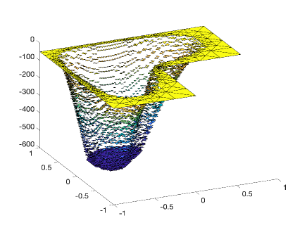
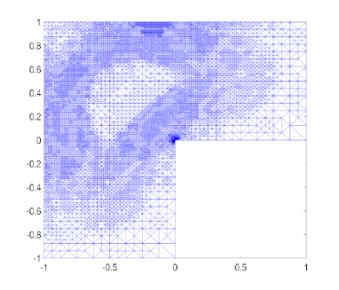
(a) Discrete control $\bar{u}_{h}$	(b) Adaptive mesh-refinement

Figure 1: Discrete control solution $\bar{u}_{h}$ (left) and the adaptive mesh-refinement (right) (at level $\ell=24$) in Example 6.2

Figure 1 shows that the significant adaptive refinement occurs near the control variable interface and the singularity point of the L-shaped domain. This is somewhat expected as the state and adjoint solutions have a singularity at the origin, and from Figure 2 it is observed that the control estimator dominates other estimators. This supports the efficiency of the adaptive estimator in the theoretical estimates obtained in the previous section. Figure 2 and Table 4 also indicate that the errors and estimators have optimal convergence in the adaptive refinement.

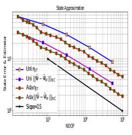
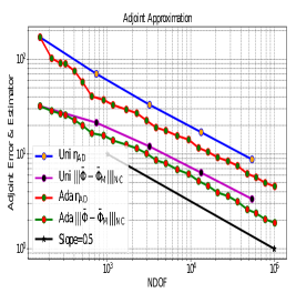
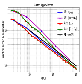
Figure 2: Convergence plot of the approximation errors and estimators with adaptive and uniform refinement for state, adjoint and control variables in Example 6.2 (State approximation (left), Adjoint approximation (Middle), Control approximation (right), Uni=Uniform refinement, Ada=Adaptive refinement).

Iteration	NDOF	$\frac{|\!|\!|\bar{\Psi}-\bar{\Psi}_{\text{M}}|\!|\!|_{\text{NC}}}{|\!|\!|\bar{\Psi}|\!|\!|_{\text{NC}}}$	Order	$\frac{|\!|\!|\bar{\Theta}-\bar{\Theta}_{\rm{M}}|\!|\!|_{\rm NC}}{|\!|\!|\bar{\Theta}|\!|\!|_{\rm NC}}$	Order	$\frac{\|\bar{u}-{\bar{u}}_{h}\|}{\|\bar{u}\|}$	Order	Total Error	Order	Ratio=T.Er/Et
0	156	1.371575	–	1.355646	–	0.760376	–	0.812881	–	1.570478
4	405	0.943121	0.51	0.961573	0.49	0.561676	0.67	0.595680	0.65	2.043008
8	1170	0.592890	0.42	0.588820	0.46	0.260259	0.88	0.289033	0.81	1.949036
12	3837	0.370235	0.59	0.365010	0.61	0.133979	0.90	0.154315	0.84	1.840881
16	12417	0.222890	0.61	0.219544	0.62	0.061046	0.70	0.074987	0.68	1.502512
20	36405	0.135407	0.51	0.132838	0.52	0.029756	0.62	0.038840	0.59	1.295190
23	78146	0.088349	0.60	0.086474	0.60	0.019719	0.50	0.025611	0.53	1.215638

Table 4: Errors and orders of convergence for state, adjoint and control variables with adaptive refinement in Example 6.2

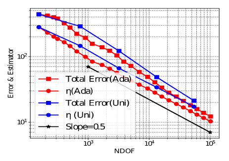
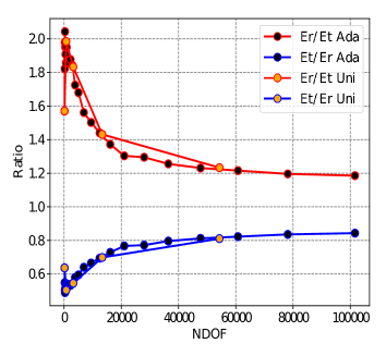
(a) Total error and estimator	(b) Efficiency and Reliability

Figure 3: Convergence plot (left), and reliability and efficiency constants (right) over uniform and adaptive refinements (right) in Example 6.2 ( Er=Total Error, Et=Complete Estimator, Uni=Uniform refinement, Ada=Adaptive refinement).

Figure 3.$(a)$ displays the convergence history of the total error and estimator; both achieve optimal convergence in adaptive refinement. Further, it can be observed that the adaptive refinements are doing better in terms of accuracy compared to the uniform refinements. Figure 3.$(b)$ illustrates that reliability and efficiency constants are approaching a constant value with mesh refinement, which is numerical evidence for the efficiency and reliability of a posteriori estimator derived in the theory section.

Acknowledgements

Asha K. Dond would like to acknowledge support from Science & Engineering Research Board (SERB), Government of India under Start-up Research Grant, Project No. SRG/2020/001027. Neela Nataraj gratefully acknowledges SERB MATRICS grant MTR/2017/000199 titled Finite element methods for nonlinear plate bending problems and optimal control problems governed by nonlinear plates and SERB POWER Fellowship SPF/2020/000019. Devika Shylaja thanks National Board for Higher Mathematics, India for the financial support towards the research work (No: 0204/3/2020/R$\&$D-II/2476).

Appendix

The detailed proofs of the a priori error estimates that are different from [19] are presented in this section.

A.4 A priori estimates

A linear mapping

For a given ${\bf g}=(g_{1},g_{2})\in{\bf V}^{\prime}$, let the linear operator $T\in{\mathcal{L}}(\text{\bf V}^{\prime},\text{\bf V})$ defined by $T{\bf g}:=\boldsymbol{\xi}=(\xi_{1},\xi_{2})\in\text{\bf V}$ solves the biharmonic system $A(\boldsymbol{\xi},\Phi)=\big{\langle}{\bf g},\Phi\big{\rangle}\mbox{ for all }\Phi\in\text{\bf V}$, that is,

$$\Delta^{2}\xi_{1}=g_{1}\,\,\mbox{ in }\Omega,\;\Delta^{2}\xi_{2}=g_{2}\mbox{ in }\Omega,\;\xi_{1}=0,\,\frac{\partial\xi_{1}}{\partial\nu}=0\text{ and }\xi_{2}=0,\,\frac{\partial\xi_{2}}{\partial\nu}=0\text{ on }\partial\Omega.$$ (A.1)

Moreover, for ${\bf{g}}\in\boldsymbol{H}^{-1}(\Omega)$, $\boldsymbol{\xi}\in\text{\bf V}\cap\boldsymbol{H}^{2+\gamma}(\Omega),\;\gamma\in(1/2,1]$, the elliptic regularity [7] result stated next holds.

$$|\!|\!|\boldsymbol{\xi}|\!|\!|_{{2}}\lesssim|\!|\!|{\bf{g}}|\!|\!|_{-1},\quad|\!|\!|\boldsymbol{\xi}|\!|\!|_{{2+\gamma}}\lesssim|\!|\!|{\bf{g}}|\!|\!|_{-1}.$$ (A.2)

For ${\bf g}\in\text{\bf V}_{\text{M}}^{\prime}$, define the bounded discrete operator $T_{\text{NC}}:\text{\bf V}_{\text{M}}^{\prime}\rightarrow\text{\bf V}_{\text{M}}$ by $T_{\text{NC}}{\bf g}:=\boldsymbol{\xi}_{\text{M}}$ where $\boldsymbol{\xi}_{\text{M}}\in\text{\bf V}_{\text{M}}$ solves the discrete problem

$${A}_{\text{NC}}(\boldsymbol{\xi}_{\text{M}},\Phi_{\text{M}})=\big{\langle}{\bf g},\Phi_{\text{M}}\big{\rangle}\;\mbox{ for all }\Phi_{\text{M}}\in\text{\bf V}_{\text{M}}.$$ (A.3)

The lemma stated next is utilized to prove the existence and uniqueness of the solution to (3.1).

Lemma A.1 (An intermediate estimate).

Let $\bar{\Psi}\in\text{\bf V}\cap{\boldsymbol{H}}^{2+\gamma}(\Omega)$ be a regular solution to (2.1). Then $\forall\epsilon>0$, $\exists h_{1}>0$ such that $\|T[\mathcal{B}^{\prime}_{\rm NC}(\bar{\Psi})]-T_{\rm NC}[\mathcal{B}_{\rm NC}^{\prime}(\Psi)]\|_{{\mathcal{L}}(\text{\bf V}+\text{\bf V}_{\rm M})}<\epsilon\;\text{ for all }\Psi\in B_{\rho_{\epsilon}}(\bar{\Psi}),$ whenever $0<h<h_{1}$.

Proof.

For ${\bf z}\in\text{\bf V}+\text{\bf V}_{\text{M}}$, (2.7) and Lemma 2.7.$(b)$ show that $\mathcal{B}_{\text{NC}}^{\prime}(\bar{\Psi})({\bf z})\in\text{\bf V}^{\prime}$ and $\mathcal{B}_{\text{NC}}^{\prime}(\bar{\Psi})({\bf z})\in\text{\bf V}_{\text{M}}^{\prime}$. For $\Psi\in\text{\bf V}+\text{\bf V}_{\text{M}}$, the definitions of $T(\bullet)$ and $T_{\text{NC}}(\bullet)$, and (A.2) imply that ${\boldsymbol{\theta}}(\bar{\Psi})=:T[\mathcal{B}^{\prime}_{\text{NC}}(\bar{\Psi})({\bf z})]\in\text{\bf V}\cap\boldsymbol{H}^{2+\gamma}(\Omega)$ and ${\boldsymbol{\theta}}_{\text{M}}(\Psi)=:T_{\text{NC}}[\mathcal{B}_{\text{NC}}^{\prime}(\Psi)({\bf z})]\in\text{\bf V}_{\text{M}}$ solve

$$A({\boldsymbol{\theta}}(\bar{\Psi}),\Phi) =\big{\langle}\mathcal{B}^{\prime}_{\text{NC}}(\bar{\Psi}){(\bf z)},\Phi\big{\rangle}\;\text{ for all }\Phi\in\text{\bf V},$$ (A.4)

$${A}_{\text{NC}}({\boldsymbol{\theta}}_{\text{M}}(\Psi),\Phi_{\text{M}}) =\langle\mathcal{B}^{\prime}_{\text{NC}}(\Psi){(\bf z)},\Phi_{\text{M}}\rangle\;\text{ for all }\Phi_{\text{M}}\in\text{\bf V}_{\text{M}}.$$ (A.5)

Let ${\boldsymbol{\theta}_{\text{M}}}(\bar{\Psi})$ and ${\boldsymbol{\theta}}^{J}_{\text{M}}(\bar{\Psi})\in\text{\bf V}_{\text{M}}$ solve the discrete problems

$$A_{\text{NC}}({\boldsymbol{\theta}_{\text{M}}}(\bar{\Psi}),\Phi_{\text{M}}) =\big{\langle}\mathcal{B}^{\prime}_{\text{NC}}(\bar{\Psi}){(\bf z)},\Phi_{\text{M}}\big{\rangle}\;\text{ for all }\Phi_{\text{M}}\in\text{\bf V}_{\text{M}},$$ (A.6)

$${A}_{\text{NC}}({\boldsymbol{\theta}}^{J}_{\text{M}}(\bar{\Psi}),\Phi_{\text{M}}) =\langle\mathcal{B}^{\prime}_{\text{NC}}(\bar{\Psi}){(\bf z)},J\Phi_{\text{M}}\rangle\;\text{ for all }\Phi_{\text{M}}\in\text{\bf V}_{\text{M}}.$$ (A.7)

A triangle inequality yields

$$|\!|\!|{\boldsymbol{\theta}}(\bar{\Psi})-{\boldsymbol{\theta}}_{\text{M}}(\Psi)|\!|\!|_{\text{NC}}\leq|\!|\!|{\boldsymbol{\theta}}(\bar{\Psi})-{\boldsymbol{\theta}}_{\text{M}}^{J}(\bar{\Psi})|\!|\!|_{\text{NC}}+|\!|\!|{\boldsymbol{\theta}}_{\text{M}}^{J}(\bar{\Psi})-{\boldsymbol{\theta}}_{\text{M}}(\bar{\Psi})|\!|\!|_{\text{NC}}+|\!|\!|{\boldsymbol{\theta}}_{\text{M}}(\bar{\Psi})-{\boldsymbol{\theta}}_{\text{M}}(\Psi)|\!|\!|_{\text{NC}}.$$ (A.8)

Notice that ${\boldsymbol{\theta}}_{\text{M}}^{J}(\bar{\Psi})$ is the Morley nonconforming solution to (A.4) for a modified right-hand side $\mathcal{B}^{\prime}_{\text{NC}}(\bar{\Psi}){(\bf z)}\circ J\in\text{\bf V}_{\text{M}}^{\prime}.$ The best-approximation result from [14, Theorem 3.2] shows

$$|\!|\!|{\boldsymbol{\theta}}(\bar{\Psi})-{\boldsymbol{\theta}}^{J}_{\text{M}}(\bar{\Psi})|\!|\!|_{\text{NC}}\leq\sqrt{1+\Lambda_{\mathrm{J}}^{2}}\;|\!|\!|(1-I_{\text{M}}){\boldsymbol{\theta}}(\bar{\Psi})|\!|\!|_{\text{NC}}.$$ (A.9)

This plus the interpolation estimate from Lemma 2.3.$(c)$, (A.2), (A.4) and Lemma 2.7.$(d)$ imply

$$|\!|\!|{\boldsymbol{\theta}}(\bar{\Psi})-{\boldsymbol{\theta}}^{J}_{\text{M}}(\bar{\Psi})|\!|\!|_{\text{NC}}\lesssim h^{\gamma}\sqrt{1+\Lambda_{\mathrm{J}}^{2}}\>|\!|\!|{\boldsymbol{\theta}}(\bar{\Psi})|\!|\!|_{2+\gamma}\lesssim h^{\gamma}|\!|\!|\mathcal{B}^{\prime}_{\text{NC}}(\bar{\Psi}){(\bf z)}|\!|\!|_{-1}\lesssim h^{\gamma}|\!|\!|\bar{\Psi}|\!|\!|_{2+\gamma}|\!|\!|{\bf z}|\!|\!|_{\text{NC}}.$$ (A.10)

The combination of (A.6) and (A.7), and (2.7) show

$$A_{\text{NC}}({\boldsymbol{\theta}_{\text{M}}}(\bar{\Psi})-{\boldsymbol{\theta}}^{J}_{\text{M}}({\bar{\Psi}}),\Phi_{\text{M}})=2B_{\text{NC}}({\bar{\Psi}},{\bf z},(1-J)\Phi_{\text{M}}).$$

The inverse inequality and Lemma 2.4.$(d)$ prove $|\!|\!|(1-J)\Phi_{\text{M}}|\!|\!|_{0,\infty}\lesssim h^{-1}|\!|\!|(1-J)\Phi_{\text{M}}|\!|\!|\lesssim h|\!|\!|\Phi_{\text{M}}|\!|\!|_{\text{NC}}$. This, Lemma 2.5.$(c)$ with test function $\Phi_{\text{M}}:={\boldsymbol{\theta}_{\text{M}}}(\bar{\Psi})-{\boldsymbol{\theta}}^{J}_{\text{M}}({\bar{\Psi}})$ and Lemma 2.7.$(a)$ imply

$$|\!|\!|{\boldsymbol{\theta}}_{\text{M}}^{J}(\bar{\Psi})-{\boldsymbol{\theta}}_{\text{M}}(\bar{\Psi})|\!|\!|_{\text{NC}}\lesssim h|\!|\!|{\bar{\Psi}}|\!|\!|_{2}|\!|\!|{\bf z}|\!|\!|_{\text{NC}}.$$ (A.11)

The combination of (A.5) and (A.6), and (2.7), Lemma 2.5.$(c)$ with test function ${\boldsymbol{\theta}_{\text{M}}}(\Psi)-{\boldsymbol{\theta}}_{\text{M}}({\bar{\Psi}})$, and Lemma 2.7.$(b)$ prove $|\!|\!|{\boldsymbol{\theta}}_{\text{M}}(\Psi)-{\boldsymbol{\theta}}_{\text{M}}(\bar{\Psi})|\!|\!|_{\text{NC}}\lesssim|\!|\!|{\bf z}|\!|\!|_{\text{NC}}|\!|\!|\Psi-{\bar{\Psi}}|\!|\!|_{\text{NC}}.$ A substitution of this and (A.10)-(A.11) in (A.8) leads to the result that for any preassigned $\epsilon>0$, $h_{1}$ and the radius $\rho_{\epsilon}>0$ can be chosen small such that for all $\Psi\in B_{\rho_{\epsilon}}(\bar{\Psi})$, $|\!|\!|T[\mathcal{B}^{\prime}_{\text{NC}}(\bar{\Psi})({\bf z})]-T_{\text{NC}}[\mathcal{B}_{\text{NC}}^{\prime}(\Psi)({\bf z})]|\!|\!|_{\text{NC}}<\epsilon|\!|\!|\bf z|\!|\!|_{\text{NC}},$ that leads to the desired estimate. ∎

The next lemma is a standard result in Banach spaces that helps to prove Lemma 4.3.

Lemma A.2.

Let $X$ be a Banach space, $A\in{\mathcal{L}}(X)$ be invertible and $B\in{\mathcal{L}}(X)$. If $\|A-B\|_{{\mathcal{L}}(X)}<1/\|A^{-1}\|_{{\mathcal{L}}(X)}$, then $B$ is invertible. If $\|A-B\|_{{\mathcal{L}}(X)}<1/(2\|A^{-1}\|_{{\mathcal{L}}(X)})$, then $\|B^{-1}\|_{{\mathcal{L}}(X)}\leq 2\|A^{-1}\|_{{\mathcal{L}}(X)}$.

The uniform boundedness result for the inverse of the linear mapping $\mathcal{F}_{\Psi_{u}}$ with a bound independent of the discretization parameter $h$ without assuming the extra regularity of $\bar{\Psi}$ is proved next. This result was used to derive the a posteriori error estimates for the adjoint variable.

Proof of Lemma 4.3.

[19, Lemma 4.3] shows that $\mathcal{F}_{\bar{\Psi}}$ is an automorphism on $\text{\bf V}+\text{\bf V}_{\rm{M}}$ if $\bar{\Psi}\in\text{\bf V}$ is a regular solution to (2.1). Also, for ${\boldsymbol{\xi}}+{\boldsymbol{\xi}}_{\text{M}}\in\text{\bf V}+\text{\bf V}_{\text{M}}$, the invertibility of $\mathcal{F}_{\bar{\Psi}}$ leads to $\mathcal{F}_{\bar{\Psi}}^{-1}({\boldsymbol{\xi}}+{\boldsymbol{\xi}}_{\text{M}})={\boldsymbol{\xi}}+{\boldsymbol{\xi}}_{\text{M}}-(\mathcal{A}+\mathcal{B}^{\prime}(\bar{\Psi})^{*})^{-1}\mathcal{B}_{\text{NC}}^{\prime}(\bar{\Psi})^{*}({\boldsymbol{\xi}}+{\boldsymbol{\xi}}_{\text{M}}).$ This, and Lemma 2.7.$(b)$ imply $\|\mathcal{F}_{\bar{\Psi}}^{-1}\|_{\mathcal{L}(\text{\bf V}+\text{\bf V}_{\rm M})}\lesssim 1+\|(\mathcal{A}+\mathcal{B}^{\prime}(\bar{\Psi})^{*})^{-1}\|_{\mathcal{L}(\text{\bf V}^{\prime},\text{\bf V})}|\!|\!|\bar{\Psi}|\!|\!|_{2}$. Since $\mathcal{A}^{*}=\mathcal{A}$ and the operator norm of an operator and its adjoint are equal, $\|(\mathcal{A}+\mathcal{B}^{\prime}(\bar{\Psi})^{*})^{-1}\|=\|(\mathcal{A}+\mathcal{B}^{\prime}(\bar{\Psi}))^{-1}\|$ and hence, there exists a constant $C$ independent of $h$ such that $\frac{1}{\|\mathcal{F}_{\bar{\Psi}}^{-1}\|_{\mathcal{L}(\text{\bf V}+\text{\bf V}_{\rm M})}}\geq C.$

For $\Phi\in\text{\bf V}+\text{\bf V}_{\text{M}}$, the definition of $\mathcal{F}_{\Psi}$ in (4.19), the boundedness property of $T(\bullet)$ and $B_{\text{NC}}(\bullet,\bullet,\bullet)$ in Lemma2.7.$(b)$ imply

$$\|\mathcal{F}_{\bar{\Psi}}(\Phi)-\mathcal{F}_{\Psi_{u}}(\Phi)\|_{\mathcal{L}(\text{\bf V}+\text{\bf V}_{\rm M})}\leq\|T[{\mathcal{B}}_{\text{NC}}^{\prime}(\bar{\Psi}-\Psi_{u})^{*}(\Phi)]\|\lesssim|\!|\!|\bar{\Psi}-\Psi_{u}|\!|\!|_{2}.$$ (A.12)

Theorem 2.1 shows $G(\bar{u})=\bar{\Psi}$, $G(u)=\Psi_{u}$ and the uniform boundedness of $|\!|\!|(\mathcal{A}+\mathcal{B}^{\prime}(\Psi_{u}))^{-1}|\!|\!|_{\mathcal{L}(\text{\bf V}^{\prime},\text{\bf V})}$ whenever $u\in{\mathcal{O}}({\bar{u}})$. Hence, for $u_{t}={u}+t(\bar{u}-u)$ and $\Psi_{t}=G(u_{t})$, mean value theorem, Theorem 2.1 and $u\in{\mathcal{O}}({\bar{u}})$ prove

$$|\!|\!|\bar{\Psi}-\Psi_{u}|\!|\!|_{2}=|\!|\!|{\int_{0}^{1}}G^{\prime}(u_{t})({\mathbf{C}}(\bar{\bf u}-{\bf{u}})))\>{\rm dt}|\!|\!|_{2}=|\!|\!|{\int_{0}^{1}}(\mathcal{A}+\mathcal{B}^{\prime}(\Psi_{t}))^{-1}({\mathbf{C}}(\bar{\bf u}-{\bf{u}}))\>{\rm dt}|\!|\!|_{2}\lesssim\|\bar{u}-{u}\|_{L^{2}(\omega)}.$$

Since $u$ is sufficently close to $\bar{u}$, (A.12) leads to

$$\|\mathcal{F}_{\bar{\Psi}}-\mathcal{F}_{\Psi_{u}}\|_{\mathcal{L}(\text{\bf V}+\text{\bf V}_{\rm M})}\leq C\leq\frac{1}{\|\mathcal{F}_{\bar{\Psi}}^{-1}\|_{\mathcal{L}(\text{\bf V}+\text{\bf V}_{\rm M})}}.$$

An application of Lemma A.2 concludes the proof. ∎

Proof of Theorem 3.3.

Step 1 (isolates a crucial term). Let $\boldsymbol{\rho}_{\text{M}}:=I_{\text{M}}\Theta_{u}-\Theta_{u,\text{M}}\in\text{\bf V}_{\text{M}}$. The triangle inequality leads to

$$|\!|\!|\Theta_{u}-\Theta_{u,\text{M}}|\!|\!|_{1,2,h}\leq|\!|\!|(1-I_{\text{M}})\Theta_{u}|\!|\!|_{1,2,h}+|\!|\!|(1-J)\boldsymbol{\rho}_{\text{M}}|\!|\!|_{1,2,h}+|\!|\!|J\boldsymbol{\rho}_{\text{M}}|\!|\!|_{1}.$$ (A.13)

Lemma 2.3.$(a)$ shows that $\Theta_{u}-I_{\text{M}}\Theta_{u}$ is orthogonal to $\Phi_{\text{M}}$ for all $\Phi_{\text{M}}\in V_{\text{M}}$ and so Lemma 2.3.$(b)$ and the Pythagoras theorem proves that

$$h^{-2}|\!|\!|\Theta_{u}-I_{\text{M}}\Theta_{u}|\!|\!|_{1,2,h}^{2}\leq C_{I}^{2}|\!|\!|\Theta_{u}-I_{\text{M}}\Theta_{u}|\!|\!|_{\text{NC}}^{2}=C_{I}^{2}(|\!|\!|\Theta_{u}-\Theta_{u,\text{M}}|\!|\!|_{\text{NC}}^{2}-|\!|\!|\boldsymbol{\rho}_{\text{M}}|\!|\!|_{\text{NC}}^{2})\leq C_{I}^{2}|\!|\!|\Theta_{u}-\Theta_{u,\text{M}}|\!|\!|_{\text{NC}}^{2}.$$ (A.14)

Lemma 2.4.$(d)$ with $v=0$ and the Pythagoras theorem in the above displayed inequality show

$$h^{-1}|\!|\!|\boldsymbol{\rho}_{\text{M}}-J\boldsymbol{\rho}_{\text{M}}|\!|\!|_{1,2,h}\leq\Lambda_{\mathrm{J}}|\!|\!|\boldsymbol{\rho}_{\text{M}}|\!|\!|_{\text{NC}}\lesssim|\!|\!|\Theta_{u}-\Theta_{u,\text{M}}|\!|\!|_{\text{NC}},$$ (A.15)

where $`\lesssim^{\prime}$ absorbs $\Lambda_{\mathrm{J}}$ and $C_{I}$. (A.13)–(A.15) concludes the first step and shows

$$|\!|\!|\Theta_{u}-\Theta_{u,\text{M}}|\!|\!|_{1,2,h}\lesssim{h}|\!|\!|\Theta_{u}-\Theta_{u,\text{M}}|\!|\!|_{\text{NC}}+|\!|\!|J\boldsymbol{\rho}_{\text{M}}|\!|\!|_{1}.$$ (A.16)

Step 2 (estimates $|\!|\!|$$J\boldsymbol{\rho}_{\text{M}}|\!|\!|_{1}$ in (A.16)). For a given ${\bf g}\in{\boldsymbol{H}}^{-1}(\Omega)$, consider the dual problem that seeks $\boldsymbol{\chi}_{\boldsymbol{g}}\in\text{\bf V}$ such that

$$A(\boldsymbol{\chi}_{\boldsymbol{g}},\Phi)+2B(\Psi_{u},\boldsymbol{\chi}_{\boldsymbol{g}},\Phi)=\langle{\bf g},\Phi\rangle\;\;\;\;\text{ for all }\Phi\in{\text{\bf V}}.$$ (A.17)

The existence of solution to (A.17) and the regularity results stated below follows from Theorem 2.1. Note that $\boldsymbol{\chi}_{\boldsymbol{g}}\in\text{\bf V}\cap{\bf H}^{2+\gamma}(\Omega)$ and

$$|\!|\!|\boldsymbol{\chi}_{\boldsymbol{g}}|\!|\!|_{2}\lesssim|\!|\!|{\bf g}|\!|\!|_{-1}\text{ and }|\!|\!|\boldsymbol{\chi}_{\boldsymbol{g}}|\!|\!|_{2+\gamma}\lesssim|\!|\!|{\bf g}|\!|\!|_{-1}.$$ (A.18)

Choose ${\bf g}=-\Delta J\boldsymbol{\rho}_{\text{M}}\in L^{2}(\Omega)$ and $\Phi=J\boldsymbol{\rho}_{\text{M}}\in\text{\bf V}$. This and elementary algebra eventually lead to

$$\|\nabla J\boldsymbol{\rho}_{\text{M}}\|^{2}=A_{\text{NC}}(\boldsymbol{\chi}_{\boldsymbol{g}},(J-1)\boldsymbol{\rho}_{\text{M}})+2(B_{\text{NC}}(\Psi_{u},\boldsymbol{\chi}_{\boldsymbol{g}},(J-1)\boldsymbol{\rho}_{\text{M}})+B_{\text{NC}}(\Psi_{u},\boldsymbol{\chi}_{\boldsymbol{g}},(I_{\text{M}}-1)\Theta_{u}))$$

$$\quad+(A_{\text{NC}}(\boldsymbol{\chi}_{\boldsymbol{g}},(I_{\text{M}}-1)\Theta_{u})+A_{\text{NC}}(\boldsymbol{\chi}_{\boldsymbol{g}},\Theta_{u}-\Theta_{u,\text{M}}))+2B_{\text{NC}}(\Psi_{u},\boldsymbol{\chi}_{\boldsymbol{g}},\Theta_{u}-\Theta_{u,\text{M}})=\sum_{i=1}^{4}T_{i}.$$ (A.19)

Step 3 estimates the terms $T_{1},\cdots,T_{4}$. Lemma 2.5.$(a)$ shows that

$$T_{1}:=A_{\text{NC}}(\boldsymbol{\chi}_{\boldsymbol{g}},(J-1)\boldsymbol{\rho}_{\text{M}})\lesssim h^{\gamma}|\!|\!|\boldsymbol{\rho}_{\text{M}}|\!|\!|_{\text{NC}}|\!|\!|\boldsymbol{\chi}_{\boldsymbol{g}}|\!|\!|_{2+\gamma}\lesssim h^{\gamma}|\!|\!|\Theta_{u}-\Theta_{u,\text{M}}|\!|\!|_{\text{NC}}|\!|\!|\boldsymbol{\chi}_{\boldsymbol{g}}|\!|\!|_{2+\gamma}$$

with (A.15) in the end. Lemmas 2.7.$(e)$, 2.4.$(d)$ with $v=\boldsymbol{\rho}_{\text{M}}$, 2.3. $(b)$, (A.14) and (A.15) imply

$$\frac{1}{2}T_{2} :=B_{\text{NC}}(\Psi_{u},\boldsymbol{\chi}_{\boldsymbol{g}},(J-1)\boldsymbol{\rho}_{\text{M}})+B_{\text{NC}}(\Psi_{u},\boldsymbol{\chi}_{\boldsymbol{g}},(I_{\text{M}}-1)\Theta_{u})\lesssim h^{2}|\!|\!|\Psi_{u}|\!|\!|_{2+\gamma}|\!|\!|\boldsymbol{\chi}_{\boldsymbol{g}}|\!|\!|_{2+\gamma}|\!|\!|\Theta_{u}-\Theta_{u,\text{M}}|\!|\!|_{\text{NC}}.$$

Simple manipulations lead to

$$T_{3} :=A_{\text{NC}}(\boldsymbol{\chi}_{\boldsymbol{g}},(I_{\text{M}}-1)\Theta_{u})+A_{\text{NC}}((1-I_{\text{M}})\boldsymbol{\chi}_{\boldsymbol{g}},\Theta_{u}-\Theta_{u,\text{M}})+A_{\text{NC}}((1-J)I_{\text{M}}\boldsymbol{\chi}_{\boldsymbol{g}},\Theta_{u}-\Theta_{u,\text{M}})$$

$$\qquad+A_{\text{NC}}(JI_{\text{M}}\boldsymbol{\chi}_{\boldsymbol{g}},\Theta_{u}-\Theta_{u,\text{M}}).$$ (A.20)

Lemma 2.3.$(a)$ shows $A_{\text{NC}}(\Phi_{\text{M}},I_{\text{M}}\Theta_{u}-\Theta_{u})=0=A_{\text{NC}}(\boldsymbol{\chi}_{\boldsymbol{g}}-I_{\text{M}}\boldsymbol{\chi}_{\boldsymbol{g}},\Phi_{\text{M}})$ for all $\Phi_{\text{M}}\in V_{\text{M}}$. This shows that the first two terms in (A.4) is

$$A_{\text{NC}}(\boldsymbol{\chi}_{\boldsymbol{g}}-I_{\text{M}}\boldsymbol{\chi}_{\boldsymbol{g}},I_{\text{M}}\Theta_{u}-\Theta_{u})+A_{\text{NC}}(\boldsymbol{\chi}_{\boldsymbol{g}}-I_{\text{M}}\boldsymbol{\chi}_{\boldsymbol{g}},\Theta_{u}-\Theta_{u,\text{M}})=0.$$

The boundedness of $A_{\text{NC}}(\bullet,\bullet)$, Lemma 2.4.$(d)$ with $v=\boldsymbol{\chi}_{\boldsymbol{g}}$ and Lemma 2.3.$(c)$ result in an estimate for the third term in (A.4) as

$$A_{\text{NC}}((1-J)I_{\text{M}}\boldsymbol{\chi}_{\boldsymbol{g}},\Theta_{u}-\Theta_{u,\text{M}})\leq h^{\gamma}|\!|\!|\boldsymbol{\chi}_{\boldsymbol{g}}|\!|\!|_{2+\gamma}|\!|\!|\Theta_{u}-\Theta_{u,\text{M}}|\!|\!|_{\text{NC}}.$$ (A.21)

Lemma 2.4.$(c)$ shows $A_{\text{NC}}(JI_{\text{M}}\boldsymbol{\chi}_{\boldsymbol{g}}-I_{\text{M}}\boldsymbol{\chi}_{\boldsymbol{g}},\Theta_{u,\text{M}})=0$. This, (3.3) and (3.4) lead to an expression for the last term in (A.4) as

$$A_{\text{NC}}(JI_{\text{M}}\boldsymbol{\chi}_{\boldsymbol{g}},\Theta_{u}-\Theta_{u,\text{M}})=A_{\text{NC}}(JI_{\text{M}}\boldsymbol{\chi}_{\boldsymbol{g}},\Theta_{u})-A_{\text{NC}}(I_{\text{M}}\boldsymbol{\chi}_{\boldsymbol{g}},\Theta_{u,\text{M}})$$

$$\qquad=(\Psi_{u}-\Psi_{d},JI_{\text{M}}\boldsymbol{\chi}_{\boldsymbol{g}})-2{B}(\Psi_{u},JI_{\text{M}}\boldsymbol{\chi}_{\boldsymbol{g}},\Theta_{u})-(\Psi_{u,\text{M}}-\Psi_{d},I_{\text{M}}\boldsymbol{\chi}_{\boldsymbol{g}})+2{B}_{\text{NC}}(\Psi_{u,\text{M}},I_{\text{M}}\boldsymbol{\chi}_{\boldsymbol{g}},\Theta_{u,\text{M}})$$

$$\qquad=(\Psi_{u}-\Psi_{d},(J-1)I_{\text{M}}\boldsymbol{\chi}_{\boldsymbol{g}})-(\Psi_{u,\text{M}}-\Psi_{u},I_{\text{M}}\boldsymbol{\chi}_{\boldsymbol{g}})-2{B}(\Psi_{u},JI_{\text{M}}\boldsymbol{\chi}_{\boldsymbol{g}},\Theta_{u})+2{B}_{\text{NC}}(\Psi_{u,\text{M}},I_{\text{M}}\boldsymbol{\chi}_{\boldsymbol{g}},\Theta_{u,\text{M}}).$$ (A.22)

Lemma 2.4.$(b)$ shows $\Pi_{0}\boldsymbol{z}=0$ for $z=(J-1)I_{\text{M}}\boldsymbol{\chi}_{\boldsymbol{g}}$. This Cauchy-Schwarz inequality, Lemmas 2.4.$(d)$ with $v=\boldsymbol{\chi}_{\boldsymbol{g}}$, Lemma 2.6.$(a)$ and 2.3.$(b)$-$(c)$ lead to the estimate for the first two terms of (A.22) as

$$\begin{split}(\Psi_{u}-\Psi_{d}-\Pi_{0}(\Psi_{u}-\Psi_{d}),(J-1)I_{\text{M}}\boldsymbol{\chi}_{\boldsymbol{g}})&\lesssim h^{2+\gamma}{\rm{osc}}_{0}(\Psi_{u}-\Psi_{d})|\!|\!|\boldsymbol{\chi}_{\boldsymbol{g}}|\!|\!|_{2+\gamma},\\ (\Psi_{u,\text{M}}-\Psi_{u},I_{\text{M}}\boldsymbol{\chi}_{\boldsymbol{g}})&\lesssim|\!|\!|\Psi_{u,\text{M}}-\Psi_{u}|\!|\!||\!|\!|\boldsymbol{\chi}_{\boldsymbol{g}}|\!|\!|_{2}.\end{split}$$ (A.23)

The terms involving trilinear forms in (A.22) are estimated now. The orthogonality property of $J$ in Lemma 2.4.$(c)$ shows that $B_{\text{NC}}(\Psi_{u,\text{M}},\boldsymbol{\chi}_{\boldsymbol{g}}-JI_{\text{M}}\boldsymbol{\chi}_{\boldsymbol{g}},{{\cal P}}_{0}\Theta_{u})=0.$ This and a simple manipulation (omitting a factor 2) lead to an expression for the last two terms of (A.22) combined with $T_{4}$ as

$$\begin{split}&{B}_{\text{NC}}(\Psi_{u}-\Psi_{u,\text{M}},(1-JI_{\text{M}})\boldsymbol{\chi}_{\boldsymbol{g}},\Theta_{u})+{B}_{\text{NC}}(\Psi_{u,\text{M}},(1-JI_{\text{M}})\boldsymbol{\chi}_{\boldsymbol{g}},(1-{{\cal P}}_{0})\Theta_{u})\\ &\qquad+{B}_{\text{NC}}(\Psi_{u,\text{M}},I_{\text{M}}\boldsymbol{\chi}_{\boldsymbol{g}},\Theta_{u,\text{M}})-B_{\text{NC}}(\Psi_{u},\boldsymbol{\chi}_{\boldsymbol{g}},\Theta_{u,\text{M}}).\end{split}$$ (A.24)

The triangle inequality with $I_{\text{M}}\boldsymbol{\chi}_{g}$, Lemmas 2.7.$(b)$, 2.3.$(c)$ and 2.4.$(d)$ with $v=\boldsymbol{\chi}_{g}$ result in

$${B}_{\text{NC}}(\Psi_{u}-\Psi_{u,\text{M}},(1-JI_{\text{M}})\boldsymbol{\chi}_{\boldsymbol{g}},\Theta_{u})\lesssim h^{\gamma}|\!|\!|\boldsymbol{\chi}_{\boldsymbol{g}}|\!|\!|_{2+\gamma}|\!|\!|\Theta_{u}|\!|\!|_{2+\gamma}|\!|\!|\Psi_{u}-\Psi_{u,\text{M}}|\!|\!|_{\text{NC}}.$$ (A.25)

Lemmas 2.7.$(a)$, 2.3.$(c)$ and 2.4.$(d)$ with $v=\boldsymbol{\chi}_{g}$ show

$${B}_{\text{NC}}(\Psi_{u,\text{M}},(1-JI_{\text{M}})\boldsymbol{\chi}_{\boldsymbol{g}},(1-{{\cal P}}_{0})\Theta_{u})\lesssim h^{\gamma}|\!|\!|\boldsymbol{\chi}_{\boldsymbol{g}}|\!|\!|_{2+\gamma}|\!|\!|\Psi_{u}|\!|\!|_{2+\gamma}|\!|\!|\Theta_{u}-{{\cal P}}_{0}\Theta_{u}|\!|\!|_{0,\infty}.$$ (A.26)

The integral mean property of $I_{\text{M}}$ in Lemma 2.3.$(a)$ shows that $B_{\text{NC}}(\Psi_{u,\text{M}},I_{\text{M}}\boldsymbol{\chi}_{\boldsymbol{g}}-\boldsymbol{\chi}_{\boldsymbol{g}},{{\cal P}}_{0}\Theta_{u})=0.$ This and a simple manipulation show that the last two terms in (A.24) can be rewritten as

$$B_{\text{NC}}(\Psi_{u}-\Psi_{u,\text{M}},(1-I_{\text{M}})\boldsymbol{\chi}_{\boldsymbol{g}},\Theta_{u,\text{M}})+B_{\text{NC}}(\Psi_{u},(1-I_{\text{M}})\boldsymbol{\chi}_{\boldsymbol{g}},\Theta_{u}-\Theta_{u,\text{M}})+B_{\text{NC}}(\Psi_{u}-\Psi_{u,\text{M}},(I_{\text{M}}-1)\boldsymbol{\chi}_{\boldsymbol{g}},\Theta_{u})$$

$$+B_{\text{NC}}(\Psi_{u,\text{M}},(I_{\text{M}}-1)\boldsymbol{\chi}_{\boldsymbol{g}},(1-{{\cal P}}_{0})\Theta_{u})+B_{\text{NC}}(\Psi_{u}-\Psi_{u,\text{M}},\boldsymbol{\chi}_{\boldsymbol{g}},\Theta_{u}-\Theta_{u,\text{M}})+B_{\text{NC}}(\Psi_{u,\text{M}}-\Psi_{u},\boldsymbol{\chi}_{\boldsymbol{g}},\Theta_{u})=\sum_{i=1}^{6}\mathbb{T}_{i}.$$ (A.27)

The terms $\mathbb{T}_{1},\cdots,\mathbb{T}_{6}$ are estimated next. The boundedness and interpolation estimates in Lemmas 2.7.$(a)-(b)$ and 2.3.$(c)$ prove

$$\mathbb{T}_{1} \lesssim h^{\gamma}|\!|\!|\boldsymbol{\chi}_{\boldsymbol{g}}|\!|\!|_{2+\gamma}|\!|\!|\Theta_{u}|\!|\!|_{2+\gamma}|\!|\!|\Psi_{u}-\Psi_{u,\text{M}}|\!|\!|_{\text{NC}},\,\mathbb{T}_{2}\lesssim h^{\gamma}|\!|\!|\boldsymbol{\chi}_{\boldsymbol{g}}|\!|\!|_{2+\gamma}|\!|\!|\Psi_{u}|\!|\!|_{2+\gamma}|\!|\!|\Theta_{u}-\Theta_{u,\text{M}}|\!|\!|_{\text{NC}}$$

$$\mathbb{T}_{3} \lesssim h^{\gamma}|\!|\!|\boldsymbol{\chi}_{\boldsymbol{g}}|\!|\!|_{2+\gamma}|\!|\!|\Theta_{u}|\!|\!|_{2+\gamma}|\!|\!|\Psi_{u}-\Psi_{u,\text{M}}|\!|\!|_{\text{NC}},\,\mathbb{T}_{4}\lesssim h^{\gamma}|\!|\!|\boldsymbol{\chi}_{\boldsymbol{g}}|\!|\!|_{2+\gamma}|\!|\!|\Psi_{u}|\!|\!|_{2+\gamma}|\!|\!|\Theta_{u}-{{\cal P}}_{0}\Theta_{u}|\!|\!|_{{0,\infty}}$$

$$\mathbb{T}_{5} \lesssim|\!|\!|\boldsymbol{\chi}_{\boldsymbol{g}}|\!|\!|_{2+\gamma}|\!|\!|\Psi_{u}-\Psi_{u,\text{M}}|\!|\!|_{\text{NC}}|\!|\!|\Theta_{u}-\Theta_{u,\text{M}}|\!|\!|_{\text{NC}}.$$

Lemma 2.8 shows $\mathbb{T}_{6}\lesssim\left(h^{\gamma}|\!|\!|\Psi_{u}-\Psi_{u,\text{M}}|\!|\!|_{\text{NC}}+|\!|\!|\Psi_{u}-\Psi_{u,\text{M}}|\!|\!|\right)|\!|\!|\boldsymbol{\chi}_{\boldsymbol{g}}|\!|\!|_{2+\gamma}|\!|\!|\Theta_{u}|\!|\!|_{2+\gamma}.$ A substitution of $\mathbb{T}_{1}$-$\mathbb{T}_{6}$ in (A.27) and the resulting estimate with (A.25) and (A.26) in (A.24) leads to a bound for the terms involving the trilinear form $B_{\text{NC}}(\bullet,\bullet,\bullet)$ as

$$|\!|\!|\boldsymbol{\chi}_{\boldsymbol{g}}|\!|\!|_{2+\gamma}\big{(}|\!|\!|\Theta_{u}|\!|\!|_{2+\gamma}\left(h^{\gamma}|\!|\!|\Psi_{u}-\Psi_{u,\text{M}}|\!|\!|_{\text{NC}}+|\!|\!|\Psi_{u}-\Psi_{u,\text{M}}|\!|\!|\right)+|\!|\!|\Psi_{u}-\Psi_{u,\text{M}}|\!|\!|_{\text{NC}}|\!|\!|\Theta_{u}-\Theta_{u,\text{M}}|\!|\!|_{\text{NC}}$$

$$\qquad+h^{\gamma}|\!|\!|\Psi_{u}|\!|\!|_{2+\gamma}(|\!|\!|\Theta_{u}-\Theta_{u,\text{M}}|\!|\!|_{\text{NC}}+|\!|\!|\Theta_{u}-{{\cal P}}_{0}\Theta_{u}|\!|\!|_{0,\infty})\big{)}.$$

This expression and (A.23) is first substituted in (A.22), the resulting expression and (A.21) is substituted in (A.4) and utilized in (A.4) with bounds for $T_{1}$ and $T_{2}$. In combination with $|\!|\!|\boldsymbol{\chi}_{\boldsymbol{g}}|\!|\!|_{2+\gamma}\lesssim|\!|\!|{\bf g}|\!|\!|_{-1}\lesssim\|\nabla J\boldsymbol{\rho}_{\text{M}}\|$ from (A.18), $|\!|\!|\Theta_{u}|\!|\!|_{2+\gamma},\,|\!|\!|\Psi_{u}|\!|\!|_{2+\gamma}\lesssim 1$ this yields

$$\|\nabla J\boldsymbol{\rho}_{\text{M}}\| \lesssim h^{\gamma}|\!|\!|\Theta_{u}|\!|\!|_{2+\gamma}|\!|\!|\Psi_{u}-\Psi_{u,\text{M}}|\!|\!|_{\text{NC}}+|\!|\!|\Psi_{u}-\Psi_{u,\text{M}}|\!|\!|_{\text{NC}}|\!|\!|\Theta_{u}-\Theta_{u,\text{M}}|\!|\!|_{\text{NC}}+(1+|\!|\!|\Theta_{u}|\!|\!|_{2+\gamma})|\!|\!|\Psi_{u}-\Psi_{u,\text{M}}|\!|\!|$$

$$\quad+h^{\gamma}(1+|\!|\!|\Psi_{u}|\!|\!|_{2+\gamma})|\!|\!|\Theta_{u}-\Theta_{u,\text{M}}|\!|\!|_{\text{NC}}+h^{\gamma}|\!|\!|\Psi_{u}|\!|\!|_{2+\gamma}|\!|\!|\Theta_{u}-{{\cal P}}_{0}\Theta_{u}|\!|\!|_{0,\infty}+h^{2+\gamma}{\rm{osc}}_{0}(\Psi_{u}-\Psi_{d}).$$

This, $|\!|\!|\Theta_{u}|\!|\!|_{2+\gamma},\,|\!|\!|\Psi_{u}|\!|\!|_{2+\gamma}\lesssim 1$ and (A.16) lead to the desired estimate. ∎

References

- [1] A. Allendes, F. Fuica, E. Otarola, and D. Quero. A posteriori error estimates for a distributed optimal control problem of the stationary Navier-Stokes equations. SIAM J. Control Optim. (Accepted for publication), arXiv: 2004.03086, 2021.
- [2] M. S. Berger. On von Kármán equations and the buckling of a thin elastic plate, I the clamped plate. Comm. Pure Appl. Math., 20:687–719, 1967.
- [3] M. S. Berger and P. C. Fife. On von Kármán equations and the buckling of a thin elastic plate. Bull. Amer. Math. Soc., 72(6):1006–1011, 1966.
- [4] M. S. Berger and P. C. Fife. Von Kármán equations and the buckling of a thin elastic plate. II plate with general edge conditions. Comm. Pure Appl. Math., 21:227–241, 1968.
- [5] H. Blum and R. Rannacher. On the boundary value problem of the biharmonic operator on domains with angular corners. Math. Methods Appl. Sci., 2(4):556–581, 1980.
- [6] S. C. Brenner, M. Neilan, A. Reiser, and L.-Y. Sung. A interior penalty method for a von Kármán plate. Numer. Math., 135(3):803–832, 2017.
- [7] S. C. Brenner and L.-Y. Sung. interior penalty methods for fourth order elliptic boundary value problems on polygonal domains. J. Sci. Comput., 22/23:83–118, 2005.
- [8] S. C. Brenner, L.-Y. Sung, H. Zhang, and Y. Zhang. A Morley finite element method for the displacement obstacle problem of clamped Kirchhoff plates. J. Comput. Appl. Math., 254:31–42, 2013.
- [9] F. Brezzi. Finite element approximations of the von Kármán equations. RAIRO Anal. Numér., 12(4):303–312, 1978.
- [10] C. Carstensen, D. Gallistl, and J. Hu. A discrete Helmholtz decomposition with Morley finite element functions and the optimality of adaptive finite element schemes. Comput. Math. Appl., 68(12, part B):2167–2181, 2014.
- [11] C. Carstensen, G. Mallik, and N. Nataraj. A priori and a posteriori error control of discontinuous Galerkin finite element methods for the von Kármán equations. IMA J. Numer. Anal., 39(1):167–200, 2019.
- [12] C. Carstensen, G. Mallik, and N. Nataraj. Nonconforming finite element discretization for semilinear problems with trilinear nonlinearity. IMA J. Numer. Anal., 41(1):164–205, 2021.
- [13] C. Carstensen and N. Nataraj. Adaptive Morley FEM for the von Kármán equations with optimal convergence rates. SIAM J. Numer. Anal., 59(2):696–719, 2021.
- [14] C. Carstensen and N. Nataraj. A priori and a posteriori error analysis of the Crouzeix–Raviart and Morley FEM with original and modified right-hand sides. Comput. Methods Appl. Math., 21(2):289–315, 2021.
- [15] C. Carstensen and S. Puttkammer. How to prove the discrete reliability for nonconforming finite element methods. J. Comput. Math, 38(1):142–175, 2020.
- [16] E. Casas, M. Mateos, and J. P. Raymond. Error estimates for the numerical approximation of a distributed control problem for the steady-state Navier-Stokes equations. SIAM J. Control Optim., 46(3):952–982 (electronic), 2007.
- [17] H. Chen, A. K. Pani, and W. Qiu. A mixed finite element scheme for biharmonic equation with variable coefficient and von Kármán equations. arXiv:2005.11734, 2020.
- [18] S. Chowdhury, T. Gudi, and A. K. Nandakumaran. A framework for the error analysis of discontinuous finite element methods for elliptic optimal control problems and applications to IP methods. Numer. Funct. Anal. Optim., 36(11):1388–1419, 2015.
- [19] S. Chowdhury, N. Nataraj, and D. Shylaja. Morley FEM for a distributed optimal control problem governed by the von Kármán equations. Comput. Methods Appl. Math., 21(1):233–262, 2021.
- [20] P. G. Ciarlet. The Finite Element Method for Elliptic Problems. North-Holland, Amsterdam, 1978.
- [21] P. G. Ciarlet. Mathematical Elasticity: Theory of Plates, volume II. North-Holland, Amsterdam, 1997.
- [22] A. Ern and J.-L. Guermond. Theory and practice of finite elements, volume 159 of Applied Mathematical Sciences. Springer-Verlag, New York, 2004.
- [23] D. Gallistl. Morley finite element method for the eigenvalues of the biharmonic operator. IMA J. Numer. Anal., pages 1–33, 2014.
- [24] P. Grisvard. Singularities in boundary value problems, volume RMA 22. Masson & Springer-Verlag, 1992.
- [25] L. Hou and J. C. Turner. Finite element approximation of optimal control problems for the von Kármán equations. Numer. Methods Partial Differential Equations, 11(1):111–125, 1995.
- [26] J. Hu and Z. C. Shi. The best norm error estimate of lower order finite element methods for the fourth order problem. J. Comput. Math., 30(5):449–460, 2012.
- [27] G. H. Knightly. An existence theorem for the von Kármán equations. Arch. Ration. Mech. Anal., 27(3):233–242, 1967.
- [28] J. L. Lions. Optimal Control of Systems governed by partial differential equations. Springer, Berlin, 1971.
- [29] G. Mallik and N. Nataraj. Conforming finite element methods for the von Kármán equations. Adv. Comput. Math., 42(5):1031–1054, 2016.
- [30] G. Mallik and N. Nataraj. A nonconforming finite element approximation for the von Kármán equations. ESAIM Math. Model. Numer. Anal., 50(2):433–454, 2016.
- [31] G. Mallik, N. Nataraj, and J.P. Raymond. Error estimates for the numerical approximation of a distributed optimal control problem governed by the von Kármán equations. ESAIM Math. Model. Numer. Anal., 52:1137–1172, 2018.
- [32] T. Miyoshi. A mixed finite element method for the solution of the von Kármán equations. Numer. Math., 26(3):255–269, 1976.
- [33] F. Tröltzsch. Optimal control of partial differential equations, volume 112 of Graduate Studies in Mathematics. American Mathematical Society, Providence, RI, 2010. Theory, methods and applications, Translated from the 2005 German original by Jürgen Sprekels.
- [34] R. Verfürth. A posteriori error estimation techniques for finite element methods. Numerical Mathematics and Scientific Computation. Oxford University Press, Oxford, 2013.