The field-angle anisotropy of proximate Kitaev systems under an in-plane magnetic field

Abstract

We have investigated the field-angle behaviors of magnetic excitations under an in-plane magnetic field for proximate Kitaev systems. By employing the exact diagonalization method in conjunction with the linear spin wave theory, we have demonstrated that the magnetic excitation gap in the polarized phase is determined by the magnon excitation at $M$ points and has a strong anisotropy with respect to the field direction in the vicinity of the critical field limit. The specific heat from this magnon excitation bears qualitatively the same anisotropic behaviors as expected one for the non-Abelian spin liquid phase in the Kitaev model and experimentally observed one of the intermediate phases in $\alpha$-RuCl₃.

I Introduction

Quantum fluctuation in frustrated spin systems can prevent any classical magnetic orders and induce exotic quantum phases such as a quantum spin liquid (QSL). The Kitaev model, the ideal $S=\frac{1}{2}$ quantum spin system with bond-directional Ising interactions in a honeycomb lattice (see Fig. 1(a)), is one of intriguing systems which host the QSL phase as a ground state. In this exactly solvable model, spin dynamics can be interpreted as free Majorana fermions in a static $Z_{2}$ flux Kitaev2006 . Majorana fermions with a gapless energy spectrum leads to the ground QSL phase and the fractionalized magnetic excitation.

Majorana fermions in the Kitaev model acquire a mass gap $\Delta$ under the magnetic field. The gapped spectrum stabilizes the topological non-Abelian spin liquid (NASL) phase characterized by the Chern number of $C=\pm 1$ and protected chiral edge modes Kitaev2006 ; Kasahara2018 . Because the mass gap is proportional to the multiplication of three components of the magnetic field with respect to local spin coordinate axes, the sign of $C$ and $\Delta$ shows strong field-angle dependency. For the in-plane field, the sign change and gap closing occur for the field applied to the bond direction between nearest neighboring (NN) spins as shown in Fig. 1(b) Yokoi2021 ; Hwang2020 ; Gordon2021 . The thermal Hall conductivity, specific heat, and magnetotropic coefficient emulate characteristic features of the Majorana energy spectrum. The field-angle behaviors of such quantities have been known as the key feature for the experimental identification of the NALS phase Yokoi2021 ; Hwang2020 ; Tanaka2020 ; Gordon2021 .

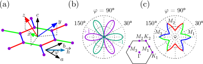
Figure 1: (a) The connection of three types of bond-dependent Ising interactions, and coordinate axes of local spins ($x$, $y$, $z$) and global honeycomb lattice ($a$, $b$, $c$) in the Kitaev model. The Ising directions in the $x$-, $y$-, and $z$-type bonds drawn with green, blue, and red lines are parallel to the $x$, $y$, and $z$ coordinate axes, respectively. The anticipated field-angle variations of (b) Majorana gap of the Kitaev model and (c) magnon gap in the polarized phase of proximate Kitaev systems under an in-plane field. $\varphi$ is the angle between the in-plane field and the $a$ axis. The radius of curves refers to the size of gap. The dark violet (sea green) curve denotes the Chern number $C=+1$ ($-1$). When the gap is determined at the $M_{1}$, $M_{2}$, and $M_{3}$ points (see the Brillouin zone in inset), the curve is drawn with green, red, and blue colors in (c), respectively.

A lot of theoretical and experimental studies have been performed to find realistic Kitaev materials Winter2017 ; Takagi2019 ; Motome2020 . Among the candidates, $\alpha$-RuCl₃ has been turned out to be the best proximate Kitaev system with dominant Kitaev interaction Jackeli2009 ; HSKim2015 . The ground state is not the QSL but the antiferromagnetic zigzag order due to the additional non-Kitaev interactions such as the Heisenberg interactions and two types of off-diagonal exchange interactions, called as $\Gamma$ and $\Gamma^{\prime}$ terms Rau2014 ; Sears2015 ; Winter2016 (see the general Hamiltonian for the proximate Kitaev system in Eq. 1). Observed magnetic continuum excitations and two-step magnetic entropy release have been regarded as the evidence of the fractionlized Majorana fermions Sandilands2015 ; Banerjee2016 ; Yadav2016 ; Banerjee2017 ; Do2017 ; Widmann2019 . Moreover, recent studies Kubota2015 ; Sears2017 ; Leahy2017 ; Baek2017 ; Wang2017 ; Zheng2017 ; Wolter2017 ; Winter2018 ; Banerjee2018 ; Kasahara2018 ; Jansa2018 ; Wellm2018 ; Balz2019 ; Gordon2019 ; HYLee2020 ; Yokoi2021 ; Tanaka2020 ; Balz2021 ; Ponomaryov2020 ; Wulferding2020 ; BHKim2020 have revealed that the zigzag order is easily destroyed when the external magnetic field is applied and the intermediate phase (IP), putative QSL, emerges between the zigzag-order phase and polarized phase. The NASL phase has been highly anticipated as the IP candidate because recent thermal Hall conductivity experiments detected the half-integer plateau and its sign signature under both in-plane and out-of-plane magnetic fields Kasahara2018 ; Yokoi2021 . Further, specific heat measurement also probed the expected field-angle anisotropy under an in-plane field Tanaka2020 . On the other side, strong sample dependency of the measured quantities has been reported Yamashita2020 . A very recent thermal conductivity experiment has reported the emergence of different types of QSL phase Czajka2021 , and the detailed thermodynamics study Bachus2021 has purported the possibility of the absence of the IP itself. All in all, the nature of the IP and/or its existence are still under debate.

In this study, we investigated the field-angle dependence of magnetic excitation and magnetic specific heat for proximate Kitaev systems under an in-plane magnetic field. Using the exact diagonalization (ED) method and linear spin wave theory (LSWT), we demonstrated that the low-energy excitation features in the polarized phase for various models relevant to $\alpha$-RuCl₃ can be interpreted in terms of the field-angle anisotropy of magnon gap, determined at one of three $M$ points depending on the field direction (see Fig. 1(c)). The magnetic specific heat dictated by this magnon dynamics shows qualitatively the same anisotropic behaviors as those in the Kitaev model. Our result suggests that the anisotropic behaviors in thermodynamic quantities alone are not a smoking gun of the intermediate NASL phase in $\alpha$-RuCl₃ under the magnetic field, but requires further considerations.

II Spin Hamiltonian

Let $\mathbf{S}_{i}^{A}$ and $\mathbf{S}_{i}^{B}$ be two base spins at the $i$-th unit cell in a honeycomb lattice. The general spin Hamiltonian of proximate Kitaev systems with first, second, and third NN interactions and external magnetic field are given as following:

$$H =\sum_{i\gamma_{1}}\mathbf{S}^{A}_{i}\cdot\tilde{\mathbf{J}}_{\gamma_{1}}\cdot\mathbf{S}^{B}_{i_{\gamma_{1}}}+\sum_{i\gamma_{3}}\mathbf{S}^{A}_{i}\cdot\tilde{\mathbf{J}}_{\gamma_{3}}\cdot\mathbf{S}^{B}_{i_{\gamma_{3}}}$$

$$+\sum_{i\gamma_{2}}\left(\mathbf{S}^{A}_{i}\cdot\tilde{\mathbf{J}}_{\gamma_{2}}\cdot\mathbf{S}^{A}_{i_{\gamma_{2}}}+\mathbf{S}^{B}_{i}\cdot\tilde{\mathbf{J}}_{\gamma_{2}}\cdot\mathbf{S}^{B}_{i_{\bar{\gamma}_{2}}}\right)$$

$$-g\mu_{B}\sum_{i}\mathbf{h}\cdot\left(\mathbf{S}_{i}^{A}+\mathbf{S}_{i}^{B}\right),$$ (1)

where $\gamma_{1}$, $\gamma_{2}$, and $\gamma_{3}$ represent the bond types of first, second, and third NN spins, respectively. $i$ and $i_{\gamma_{n}}$ are the unit cell indices of two spins in the $\gamma_{n}$ bond (see Fig. 2(a)). $\gamma$ ($=x,y,z$) can be characterized by three coordinate axes of spins. $\bar{\gamma}_{2}$ refers to the bond with the opposite direction of the $\gamma_{2}$ bond. $g$ is the $g$ factor of spins and $\mu_{B}$ is the Bohr magneton. $\tilde{\mathbf{J}}_{\gamma_{n}}$ is the superexchange dyadic tensor of the $\gamma$-type $n$-th NN bond defined as

$$\tilde{\mathbf{J}}_{\gamma_{n}} =J_{n}\hat{\alpha}\hat{\alpha}+J_{n}\hat{\beta}\hat{\beta}+(J_{n}+K_{n})\hat{\gamma}\hat{\gamma}+\Gamma_{n}\left(\hat{\alpha}\hat{\beta}+\hat{\beta}\hat{\alpha}\right)$$

$$+\Gamma^{\prime}_{n}\left(\hat{\alpha}\hat{\gamma}+\hat{\gamma}\hat{\alpha}+\hat{\gamma}\hat{\beta}+\hat{\beta}\hat{\gamma}\right),$$ (2)

where $\alpha$, $\beta$, and $\gamma$ are cyclically ordered coordinate axes of local spins and $\hat{\gamma}$ is the unit vector along the $\gamma$ axis. $J_{n}$, $K_{n}$, $\Gamma_{n}$, and $\Gamma^{\prime}_{n}$ are the exchange parameters of the Heisenberg interaction, Kitaev interaction, and two types of off-diagonal interactions between $n$-th NN spins, respectively. The global coordinate axes $a$, $b$, and $c$ can be determined so that the $a$ ($b$) axis is parallel (perpendicular) to the displacement between two spins in the $z_{1}$-type bond and the $c$ axis is normal to the honeycomb lattice (See Fig. 1(a)). Unit vectors $\hat{a}$, $\hat{b}$, and $\hat{c}$ are given as $\hat{a}=\frac{\hat{x}+\hat{y}-2\hat{z}}{\sqrt{6}}$, $\hat{b}=\frac{-\hat{x}+\hat{y}}{\sqrt{2}}$, and $\hat{c}=\frac{\hat{x}+\hat{y}+\hat{z}}{\sqrt{3}}$ in terms of local spin coordinate axes. In the text, the exchange parameters between first NN spins are simply denoted as $J$, $K$, $\Gamma$, and $\Gamma^{\prime}$ omitting neighbor indices.

Table 1: Some magnetic models have been proposed for proximate Kitaev system $\alpha$-RuCl₃ before. The unit of magnetic exchange interactions is meV.

Model	$J$	$K$	$\Gamma$	$\Gamma^{\prime}$	$K_{2}$	$J_{3}$	Ref.
1	$-4.6$	$7.0$					[Banerjee2016, ]
2	$-1.53$	$-6.55$	$5.25$	$-0.95$			[HSKim2015, ]
3	$-2.7$	$-10$	$10.6$	$-0.9$			[Sears2020, ]
4	$-0.5$	$-5.0$	$2.5$			0.5	[Winter2018, ]
5	$-1.5$	$-10$	$8.8$			0.4	[Sears2020, ]
6	$-1.3$	$-15.1$	$10.1$	$-0.1175$	$-0.68$	$0.9$	[Laurell2020, ]
7	$-4.0$	$-10.8$	$5.2$	$2.9$		$3.26$	[Maksimov2020, ]

Various magnetic models have been proposed to describe the magnetic and thermal properties of proximate Kitaev system $\alpha$-RuCl₃ by setting the Kitaev interaction between first NN spins to be dominant and specific parameters to be zero in Eq. 2 Yadav2016 ; Winter2016 ; Winter2017 ; HSKim2015 ; Banerjee2016 ; Ran2017 ; Gordon2019 ; Laurell2020 ; Hou2017 ; Eichstaedt2019 ; Sears2020 ; Laurell2020 ; Maksimov2020 ; Suzuki2021 . A few representative models, which have been proposed for $\alpha$-RuCl₃ before, are presented in Table 1.

To investigate the field-angle anisotropy of proximate Kitaev model under an in-plane magnetic field, we first adopted the simple $K$-$\Gamma$-$J_{3}$ model with $J_{3}/|K|=\Gamma/|K|=0.1$ and $K<0$, which also accounts for the magnetic phase of the system well. Then we extended our study to more realistic models presented in Table 1.

III ED calculation

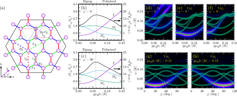
Figure 2: (a) Schematic diagram of a periodic 24-site cluster. ‘A’ and ‘B’ refer to two base sites of a honeycomb lattice, respectively. The bonds between first, second, and third nearest neighboring (NN) spins are drawn with solid, fine dotted, and thick dotted lines, respectively. $x$, $y$, and $z$ types of bonds are highlighted by green, blue, and red colors, respectively. $x_{1}$, $x_{2}$, and $x_{3}$ mean the $x$-type first, second, and third NN bonds, respectively. Static spin structure factors of the ground state $\left<\mathbf{S}_{-\mathbf{q}}\cdot\mathbf{S}_{\mathbf{q}}\right>$ at $\mathbf{q}=\Gamma$, $M_{1}$, and $M_{2}$ points under the (b) $a$- and (c) $b$-axis fields ($\varphi=0^{\circ}$ and $\varphi=90^{\circ}$). Solid black curves in (b) and (c) represent the second derivatives of the ground state energy ($-d^{2}E_{g}/dh^{2}$) with respect to the field strength for given field direction. The critical field strength of the phase transition from the zigzag order to the polarized phase are indicated with vertical dotted line. Dynamical spin structure factors (DSSFs) $\chi_{\mathbf{q}}(\omega)$ of the $K$-$\Gamma$-$J_{3}$ model with $J_{3}/|K|=\Gamma/|K|=0.1$ and $K<0$ at (d) $\Gamma$ (e) $M_{1}$, and (f) $M_{2}$ points as a function of the field strength $h$ when a magnetic field is along the $a$ axis. The $\Gamma$, $K_{1}$, $M_{1}$, and $M_{2}$ points are defined in Fig. 1. DSSF at (g) $M_{1}$ and (h) $M_{2}$ points as a function of the field angle $\varphi$, the angle between the in-plane field and the $a$ axis, when $g\mu_{B}h/|K|=0.12$. All results are calculated by the ED method with a periodic 24-site cluster. The circle data represent the lowest seven excitation energies calculated by the thick-restarted Lanczos method Wu2000 .

Employing the ED method with the periodic $24$-site cluster as shown in Fig. 2(a), we investigated the magnetic phase transition of the $K$-$\Gamma$-$J_{3}$ model with $J_{3}/|K|=\Gamma/|K|=0.1$ and $K<0$ under an in-plane field. With the help of the thick-restarted Lanczos method Wu2000 , we obtained the ground state $\left|\Psi_{g}\right>$ and its energy $E_{g}$. Figure 2(b) and (c) present the static spin structure factors (SSSFs) $\left<\Psi_{g}\right|\mathbf{S}_{-\mathbf{q}}\cdot\mathbf{S}_{\mathbf{q}}\left|\Psi_{g}\right>$ at $\mathbf{q}=\Gamma$, $M_{1}$, and $M_{2}$ points (see the Brillouin zone in Fig. 1) for the $a$- and $b$-axis fields. $\mathbf{S}_{\mathbf{q}}$ is defined as $\mathbf{S}_{\mathbf{q}}=\frac{1}{\sqrt{N}}\sum_{j=1}^{N}{\rm e}^{-i\mathbf{q}\cdot\mathbf{r}_{j}}\mathbf{S}_{j}$, where $\mathbf{r}_{j}$ is the position vector of the $j$-th spin $\mathbf{S}_{j}$ in the honeycomb lattice and $N$ is the total number of spin sites. Note that the SSSFs at $\Gamma$ and three $M$ points characterize the polarized phase and three types of the zigzag order, respectively. Results indicate that the magnetic phase transition happens from the zigzag-order phase to polarized phase at around $g\mu_{B}h/|K|=0.1$ without hosting any IP under both $a$- and $b$-axis fields. In the ED calculation, the IP is only feasible for an out-of-plane field. For the $c$-axis field, the IP appears in the range of $0.396\leq g\mu_{B}h/|K|\leq 0.416$ (not shown here).

Further, we numerically explored the magnetic excitation features as a function of strength and direction of an in-plane magnetic field by calculating the dynamical spin structure factor (DSSF) $\chi_{\mathbf{q}}(\omega)$ as following:

$$\chi_{\mathbf{q}}(\omega)=-\frac{1}{\pi}\textrm{Im}\sum_{\nu}\left<\Psi_{g}\right|S_{\mathbf{-q},\nu}\frac{1}{\omega-H+E_{g}+i\delta}S_{\mathbf{q},\nu}\left|\Psi_{g}\right>,$$ (3)

where $S_{\mathbf{q},\nu}$ is the $\nu$ ($=x,y,z$) component of $\mathbf{S}_{\mathbf{q}}$ and $\delta$ ($=0.01|K|$) is the broadening parameter. When a magnetic field is applied along the $a$ axis ($\varphi=0^{\circ}$, where $\varphi$ is the angle between the in-plane field and the $a$ axis), the minimum excitation energies at both the $\Gamma$ and $M_{1}$ points decrease in a weak field limit but they start to increase at around the critical field corresponding to the zigzag order to the polarized phase transition. The excitation gap is determined at the $M_{1}$ point regardless of the field strength. In contrast, the minimum excitation energy at the $M_{2}$ point, originally degenerate with those at other $M$ points without the field, monotonically increases with losing its spectral weight when the field strength increases (see Fig. 2(d), (e), and (f)).

The $24$-site cluster has the dihedral $D_{3}$ symmetry which includes both $C_{2}$ rotation along three NN bond directions and $C_{3}$ rotation along the $c$ axis. Due to the $C_{2}$ rotation symmetry, the excitation spectra at three $M$ points have the $180^{\circ}$ periodicity for the field angle $\varphi$. In addition, the excitation spectra at three $M$ points have a cyclic relation under the $C_{3}$ rotation. These symmetric features are well captured in the polarized phase region of $g\mu_{B}h/|K|=0.12$ as shown in Fig. 2(g) and (h). The DSSFs $\chi_{M_{1}}$, $\chi_{M_{2}}$, and $\chi_{M_{3}}$ have the $180^{\circ}$ periodicity, and the excitation gap is determined from $\chi_{M_{1}}$, $\chi_{M_{2}}$, and $\chi_{M_{3}}$ when the field angle $\varphi$ is located at $0^{\circ}\leq\varphi\leq 60^{\circ}$, $60^{\circ}\leq\varphi\leq 120^{\circ}$, and $120^{\circ}\leq\varphi\leq 180^{\circ}$, respectively. The minima of the excitation gap appear whenever a magnetic field is parallel to one out of three NN bond directions ($\varphi=(2n+1)\times 30^{\circ}$ where $n$ is the integer number).

As shown in Fig. 2(g) and (h), the excitation gap at $\varphi=0^{\circ}$ is higher than that at $\varphi=90^{\circ}$, which means that the magnetic entropy under the $b$-axis field ($\varphi=90^{\circ}$) is easier to be thermally populated in a low-temperature limit than the $a$-axis-field case ($\varphi=0^{\circ}$). Hence, the magnetic specific heat $C_{m}$ has a lower gap for the field along the $b$ axis than the $a$ axis, which is well captured in Fig. 3(a). Here we employed the $K$-$\Gamma$-$J_{3}$ model with $g\mu_{B}h/|K|=0.12$ (see Appendix A for the calculation detail). Also, we found the six-fold symmetricity of $C_{m}$ upon the field angle $\varphi$ for the low-temperature case ($k_{B}T/|K|\lesssim 0.01$) as shown in Fig. 3(b). $C_{m}$ periodically varies with minimum values at $\varphi=n\times 60^{\circ}$ and maximum values at $\varphi=(2n+1)\times 30^{\circ}$. The anisotropic behaviors are suppressed when the field strength is increased from $g\mu_{B}h/|K|=0.12$ to $0.2$, which is consistent with the experimental observations of $\alpha$-RuCl₃ Tanaka2020 .

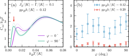
Figure 3: (a) Theoretical specific heat $C_{m}$ of the $K$-$\Gamma$-$J_{3}$ model with $J_{3}/|K|=\Gamma/|K|=0.1$ and $K<0$ when $g\mu_{B}h/|K|=0.12$ under the $a$- and $b$-axis fields ($\varphi=0^{\circ}$ and $\varphi=90^{\circ}$). (b) $\varphi$ variation of the specific heat for $g\mu_{B}h/|K|=0.12$ and $0.2$ at $k_{B}T/|K|=0.008$ indicated by red arrow in (a). Results are calculated by the finite temperature Lanczos method (FTLM) Jaklic2000 ; Aichhorn2003 with a periodic 24-site cluster. Dotted lines in (a) and error bars in (b) represent standard deviations of FTLM calculation (see Appendix A for the detail).

IV Spin wave theory

To get further insight on the field-angle anisotropy under an in-plane magnetic field, we examined the excitation features in terms of the LSWT (see the detail in Appendix B). We performed the LSWT calculation within the polarized phase in which all spins are ferromagnetically ordered along the field direction. By reducing the field strength from the infinity, we traced the variation of magnon dispersions in the $K$-$\Gamma$-$J_{3}$ model.

In the classical magnetic phase diagram for $J_{3}/|K|=\Gamma/|K|=0.1$, the polarized phase is stabilized when $g\mu_{B}h/|K|$ is larger than about $0.295$ ($0.305$) for the $a$-axis ($b$-axis) field as shown in the Fig. 4 (see the calculation detail in Appendix C). The calculated magnon bands are always gapped in this field limit. The gap is monotonically diminished as the field strength is reduced. Eventually, the magnon bands condense at the $M_{2,3}$ points ($M_{1}$ point) under the $a$-axis ($b$-axis) field with the critical field strength of $g\mu_{B}h/|K|=0.2930$ ($0.3048$) (see Fig. 4 and Fig. 5(a)). For the field-angle dependency, as analogous to the previous DSSFs, the magnon bands have the $D_{3}$ character in the critical field limit: the low-lying excitation gap at $0^{\circ}\leq\varphi\leq 60^{\circ}$, $60^{\circ}\leq\varphi\leq 120^{\circ}$, and $120^{\circ}\leq\varphi\leq 180^{\circ}$, is determined at $M_{1}$, $M_{2}$, and $M_{3}$ points, respectively. The gap minima are located at $\varphi=(2n+1)\times 30^{\circ}$ as shown in Fig. 5(b).

Figure 4: Expectation values of the order parameters of the zigzag order and polarized phase of the classical $K$-$\Gamma$-$J_{3}$ model with $\Gamma/|K|=J_{3}/|K|=0.1$ and $K<0$ under the (a) $a$- and (b) $b$-aixs fields ($\varphi=0^{\circ}$ and $\varphi=90^{\circ}$). They are calculated with the classical Monte Carlo method at $k_{B}T/|K|=0.02$. The lowest magnon energies at the $M_{1}$ and $M_{2}$ points in the polarized phase are presented with orange and red lines, respectively. Vertical dotted lines represent the phase boundary.

Based on the magnon dispersions, we calculated the magnon specific heat $C_{m}$ which is attributed to one-magnon excitation. Figure 5(c) presents $C_{m}$ behaviors as a function of temperature $T$ under both $a$- and $b$-axis fields at the critical field strength of $g\mu_{B}h/|K|=0.3048$. For the $b$-axis field, the $C_{m}$ is gapless since the magnon is gappless at the critical strength, while it is still gapped for the $a$-axis field. The six-fold symmetric behaviors of $C_{m}$, at low $T$, can be also observed such that minimum and maximum values at $\varphi=n\times 60^{\circ}$ and $(2n+1)\times 30^{\circ}$ as shown in Fig. 5(d). The anisotropic behaviors are progressively suppressed as the field strength is increased beyond the critical value. All behaviors are consistent with both results of ED calculation and experimental observations of $\alpha$-RuCl₃ Tanaka2020 .

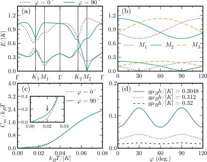
Figure 5: Magnon bands and magnon specific heats of the $K$-$\Gamma$-$J_{3}$ model with $J_{3}/|K|=0.1$, $\Gamma/|K|=0.1$, and $K<0$ when $g\mu_{B}h/|K|=0.3048$. (a) Magnon bands under the $a$- and $b$-axis fields ($\varphi=0^{\circ}$ and $\varphi=90^{\circ}$). (b) Magnon bands as a function of $\varphi$ at the $M_{1}$, $M_{2}$, and $M_{3}$ points. (c) Specific heats as a function of $T$ under the $a$- and $b$-axis fields. Zoom-in of the low-temperature specific heat is presented in the inset of (c). (d) Specific heats as a function of $\varphi$ when $k_{B}T/|K|=0.02$ indicated by red arrow in the inset of (c). All data are calculated by the linear spin-wave theory.

V Application to $\alpha$-RuCl₃

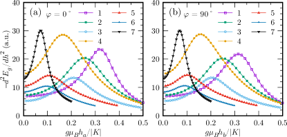
Figure 6: Second derivative of the ground state energy with respect to the field strength ($-d^{2}E_{g}/dh^{2}$) for models 1 to 7 in Table 1 under (a) $a$- and (b) $b$-axis fields ($\varphi=0^{\circ}$ and $\varphi=90^{\circ}$). The ground state energy is obtained with the ED calculation of the periodic 24-site cluster shown in Fig. 2(a).

We extended our study to a few representative models (models 1 to 7), which have been proposed for the magnetic and thermal properties of $\alpha$-RuCl₃, as shown in Table 1.

We investigated their magnetic phase transition under an in-plane magnetic field. As shown in Fig. 6, the second derivative of their ground state energy with respect to the field strength ($-d^{2}E_{g}/dh^{2}$) shows single peak in the ED calculation. All models seem to exhibit the phase transition from the zigzag order to the polarized phase without hosting any IP under both $a$- and $b$-axis fields like the $K$-$\Gamma$-$J_{3}$ model. However, the ED calculation with small-size cluster is limited due to the finite size effect. The absence of IP under an in-plane field is still questionable.

We examined the behaviors of DSSFs, magnon dispersions, and magnon specific heat under both $a$- and $b$-axis fields for models 1–7. Results are presented in Fig. 7 and 8. Overall, we found all considered models bear the essentially same field-angle anisotropy. More specifically, the DSSF, magnon condensation, and magnon specific heat behaviors under an in-plane magnetic field are the same between models 1–4 and the $K$-$\Gamma$-$J_{3}$ model (see Fig. 7). Small differences in DSSFs and/or magnon condensation are found for models 5–7: (i) DSSFs $\chi_{M_{1}}$ and $\chi_{M_{2}}$ do not determine the excitation gap for $a$- and $b$-axis fields for model 7. (ii) The magnon condensation point is slightly shifted from the $M_{2}$ to $\Gamma$ points under the $b$-field for models 5 and 6. Still, the quantitative features remain very similar (see Fig. 8). Therefore, our results suggest the potential role of magnon dynamics in explaining the field-angle anisotropy of low-temperature thermal properties for $\alpha$-RuCl₃.

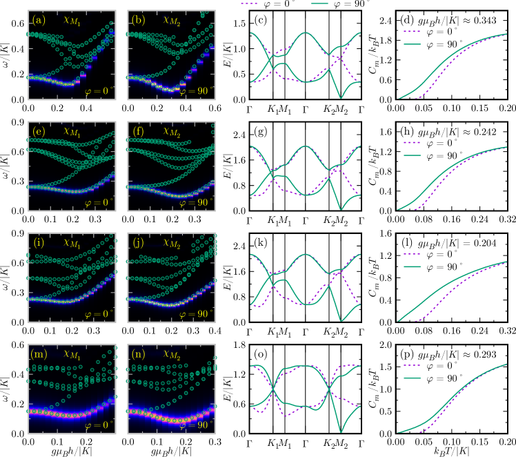
Figure 7: Dynamical spin structure factors $\chi_{M_{1}}(\omega)$ under the $a$-axis field ($\varphi=0^{\circ}$) and $\chi_{M_{2}}(\omega)$ under the $b$-axis field ($\varphi=90^{\circ}$), and the magnon dispersions and magnon specific heats under the $a$- and $b$-axis fields at the critical field strength for (a) – (d) model 1, (e) – (h) model 2, (i) – (l) model 3, and (m) – (p) model 4 in Table 1. The critical field strength, at which the magnon bands condense under the $b$-axis field, is $g\mu_{B}h/|K|\approx 0.343$ for model 1, $0.242$ for model 2, $0.204$ for model 3, and $0.293$ for model 4. Circle data in (a), (b), (e), (f), (i), (j), (m), and (p) represent the lowest seven excitation energies calculated by the thick-restarted Lanczos method Wu2000 .

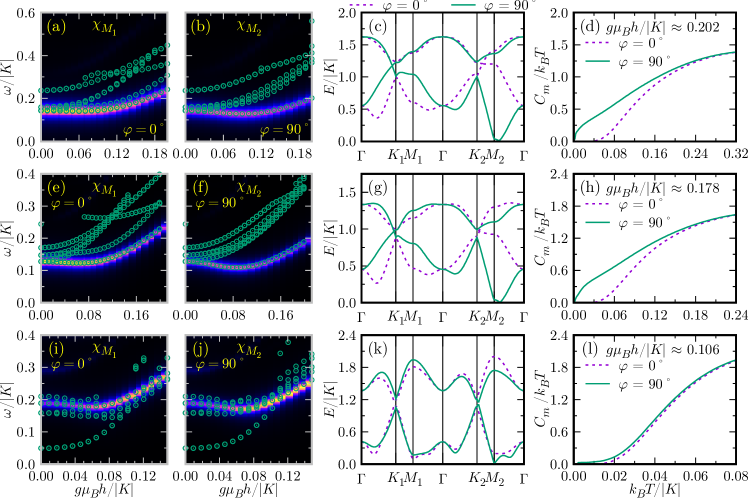
Figure 8: Dynamical spin structure factors $\chi_{M_{1}}(\omega)$ under the $a$-axis field ($\varphi=0^{\circ}$) and $\chi_{M_{2}}(\omega)$ under the $b$-axis field ($\varphi=90^{\circ}$), and the magnon dispersions and magnon specific heats under the $a$- and $b$-axis fields at the critical field strength for (a) – (d) model 5, (e) – (h) model 6, and (i) – (l) model 7 in Table 1. The critical field strength, at which the magnon bands condense under the $b$-axis field, is $g\mu_{B}h/|K|\approx 0.202$ for model 5, $0.178$ for model 6, and $0.106$ for model 7. Circle data in (a), (b), (e), (f), (i), and (j) represent the lowest seven excitation energies calculated by the thick-restarted Lanczos method Wu2000 .

Previously, we proposed the $K$-$J_{3}$ model with $K<0$ and $J_{3}>0$ as the simplest model to account for the IP for the $a$-axis field BHKim2020 , where, we found the magnon simultaneously condenses at both the $M_{1}$ and $M_{2}$ points with the suppression of the anisotropy in the magnon specific heat $C_{m}(T)$ (see Appendix D). Hence, we conjecture that the $\Gamma$-term plays a significant role in the in-plane anisotropic feature in the proximate Kitaev model with ferromagnetic $K$ ($K<0$).

VI Discussion

In contrast with the ED calculations of various models to show no IP, plausible evidence of intermediate NASL phase such as the half plateau thermal Hall conductivity and field-angle anisotropy of specific heat has been reported in $\alpha$-RuCl₃ in the intermediate range of the $a$-axis field ($7\sim 10$ T) Yokoi2021 ; Tanaka2020 . The lower bound field is coincident with the critical field at which the zigzag order totally disappears. However, the upper phase boundary is not evident. The thermodynamic quantities such as magnetic susceptibility, specific heat, and magnetic Grüneisen parameter show no clear anomalies at around the upper field Balz2019 ; Balz2021 ; Bachus2021 . Moreover, the recent electron spin resonance (ESR) experiment unveiled that the single-magnon excitation is present across the upper field Ponomaryov2020 . The magnon dynamics of polarized phase is certainly anticipated to emerge even for the intermediate region of $\alpha$-RuCl₃.

An important remark on the magnon dynamics of the polarized phase is that the excitation gap is determined at not the $\Gamma$ point but $M$ points in contrast with the NASL phase in which the magnetic excitation gap appears at the $\Gamma$ point. The momentum of the excitation gap could be good measure the origin of the field-angle anisotropy of specific heat. The full magnetic excitation features, which can be measured by the inelastic neutron scattering (INS) and resonant inelastic x-ray scattering experiments, are crucial for determining the nature/existence of IP of $\alpha$-RuCl₃. According to recent INS, Raman spectroscopy, and ESR experiments Banerjee2017 ; Wulferding2020 ; Ponomaryov2017 ; Ponomaryov2020 , the minimum excitation energy at the $\Gamma$ point evidently decreases before the phase boundary and increases again after the boundary. In the experimental resolution, however, it is hardly resolved whether the gap is genuinely closed or not. It was also verified that the excitation energy at the $M_{2}$ point in the INS is almost constant in the zigzag ordering limit and that it increases by losing its spectral weight after the phase boundary. This behavior is quite similar to our ED calculation. However, only magnetic excitation along the $\Gamma$-$M_{2}$ line under the $a$-axis field has been reported in the hitherto INS measurement. The momentum resolved excitations except for the $\Gamma$ point are limited in Raman spectroscopy and ESR experiments. Experimental observations with different momentum lines and various field directions are highly required.

The recent theoretical study has pointed out that the magnon topology in the polarized phase of the proximate Kitaev system can give rise to the field-angle variation in the thermal Hall conductivity which has the same sign structure as that in the NASL phase Chern2021 . Our result supports novel significant feature of this magnon dynamics. Thus, the field-angle anisotropy of both specific heat and thermal Hall conductivity cannot be taken as a key evidence for the NASL phase. For the ultimate identification, one should test more comprehensively a few characteristic features which are inherent to Majorana fermion dynamics, e.g., the continuum excitation at the $\Gamma$ point, the half-integer plateau of thermal Hall conductivity under the $a$-axis field, and $T^{2}$-behavior of the specific heat at low temperature under the $b$-axis field.

VII Conclusion

Based on the numerical ED calculation and LSWT analysis, we have explored the field-angle anisotropy of proximate Kitaev systems under an in-plane magnetic field. We have found that the low-lying excitation gap, interpreted as the magnon excitation in the polarized phase, is determined at not the $\Gamma$ but $M$ points in the vicinity of the phase boundary between the zigzag order and polarized phase. Also, the excitation gap has the $60^{\circ}$ periodicity for the field angle with its minimum when the field is along the NN bond direction. The anisotropy of the low-energy magnon gap can reproduce the field-angle anisotropy of the specific heat, which was considered a hallmark of the NASL phase. Our results provide a novel insight into determining the nature/existence of IP in the field-induced phase transition of $\alpha$-RuCl₃.

Appendix A Finite-temperature Lanczos method

We performed the finite-temperature Lanczos method (FTLM) Jaklic2000 ; Aichhorn2003 to calculate the magnetic specific heat of proximate Kitaev systems with the 24-site cluster. The specific heat at temperature $T$ is given as

$$C_{m}(T)=\frac{k_{B}}{N(k_{B}T)^{2}}\left(\left<H^{2}\right>-\left<H\right>^{2}\right),$$ (4)

where $N$ is the total number of spin sites, $H$ is the spin Hamiltonian, and $k_{B}$ is the Boltzmann constant, respectively. The expectation values of $H$ and $H^{2}$ can be approximately estimated as following:

$$\left<H\right>\approx\frac{N_{st}}{ZN_{sc}}\sum_{r=1}^{N_{sc}}\sum_{m=0}^{N_{L}}\varepsilon_{r,m}e^{-\beta\varepsilon_{r,m}},$$ (5)

$$\left<H^{2}\right>\approx\frac{N_{st}}{ZN_{sc}}\sum_{r=1}^{N_{sc}}\sum_{m=0}^{N_{L}}(\varepsilon_{r,m})^{2}e^{-\beta\varepsilon_{r,m}},$$ (6)

where $N_{st}$, $N_{sc}$, and $N_{L}$ are the size of Hilbert space, the number of initial random states, and the number of Lanczos iteration steps, respectively. $\varepsilon_{r,m}$ refers to the $m$-th eigenvalue calculated by the Lanczos method with the $r$-th initial random state. $Z$ is the partition function which is also approximately calculated as

$$Z\approx\frac{N_{st}}{N_{sc}}\sum_{r=1}^{N_{sc}}\sum_{m=0}^{N_{L}}e^{-\beta\varepsilon_{r,m}}\left|\left<\psi_{r,m}|\phi_{r}\right>\right|^{2},$$ (7)

where $\left|\phi_{r}\right>$ is the normalized $r$-th initial random state and $\left|\psi_{r,m}\right>$ is the $m$-th eigenstate calculated by the Lanczos method with the initial state $\left|\phi_{r}\right>$. In the calculation, we set $N_{sc}=250$ and $N_{L}=200$.

Appendix B Linear spin wave theory

In the polarized phase, all spins are ferromagnetically ordered along the magnetic field direction. We performed the liner spin wave theory (LSWT) assuming that an in-plane magnetic field is applied away from the $a$ axis with the field angle $\varphi$. According to the Holstein-Primakoff transformation, the spin operators can be written in terms of two bosonic operators as following:

$$S_{ix^{\prime}}^{A} =\frac{\sqrt{2S-a_{i}^{\dagger}a_{i}}a_{i}+a_{i}^{\dagger}\sqrt{2S-a_{i}^{\dagger}a_{i}}}{2}$$

$$\approx\sqrt{\frac{S}{2}}\left(a_{i}+a_{i}^{\dagger}\right),$$ (8a)

$$S_{iy^{\prime}}^{A} =\frac{\sqrt{2S-a_{i}^{\dagger}a_{i}}a_{i}-a_{i}^{\dagger}\sqrt{2S-a_{i}^{\dagger}a_{i}}}{2i}$$

$$\approx-i\sqrt{\frac{S}{2}}\left(a_{i}-a_{i}^{\dagger}\right),$$ (8b)

$$S_{iz^{\prime}}^{A}=S-a_{i}^{\dagger}a_{i},$$ (8c)

$$S_{ix^{\prime}}^{B}\approx\sqrt{\frac{S}{2}}\left(b_{i}+b_{i}^{\dagger}\right),$$ (8d)

$$S_{iy^{\prime}}^{B}\approx-i\sqrt{\frac{S}{2}}\left(b_{i}-b_{i}^{\dagger}\right),$$ (8e)

$$S_{iz^{\prime}}^{B}=S-b_{i}^{\dagger}b_{i},$$ (8f)

where $a^{\dagger}_{i}$ ($a_{i}$) and $b^{\dagger}_{i}$ ($b_{i}$) are the bosonic creation (annihilation) operators of magnons at the $i$-th $A$ and $B$ sublattices, respectively, and $x^{\prime}$, $y^{\prime}$, and $z^{\prime}$ are coordinate axes defined as

$$\hat{x}^{\prime}=-\hat{c},$$ (9a)

$$\hat{y}^{\prime}=-\sin\varphi\hat{a}+\cos\varphi\hat{b},$$ (9b)

$$\hat{z}^{\prime}=\cos\varphi\hat{a}+\sin\varphi\hat{b},$$ (9c)

where $a$, $b$, and $c$ are global coordinate axes of the lattice.

The magnetic interactions between first, second, and third NN spins in Eq. 1 can be approximately expressed in terms of the bosonic operators as following:

$$\mathbf{S}^{A}_{i}\cdot\tilde{\mathbf{J}}_{\gamma_{n}}\cdot\mathbf{S}^{B}_{i_{\gamma_{n}}}\approx Sc_{\gamma_{n}}(\varphi)\left(S-a_{i}^{\dagger}a_{i}-b_{i_{\gamma_{n}}}^{\dagger}b_{i_{\gamma_{n}}}\right)\\ +Sd_{\gamma_{n}}(\varphi)a_{i}^{\dagger}b_{i_{\gamma_{n}}}^{\dagger}+Sd_{\gamma_{n}}(\varphi)^{*}a_{i}b_{i_{\gamma_{n}}}\\ +Sh_{\gamma_{n}}(\varphi)a_{i}^{\dagger}b_{i_{\gamma_{n}}}+Sh_{\gamma_{n}}(\varphi)^{*}a_{i}b_{i_{\gamma_{n}}}^{\dagger},$$ (10)

$$\mathbf{S}^{A}_{i}\cdot\tilde{\mathbf{J}}_{\gamma_{2}}(\varphi)\cdot\mathbf{S}^{A}_{i_{\gamma_{2}}}+\mathbf{S}^{B}_{i}\cdot\tilde{\mathbf{J}}_{\gamma_{2}}(\varphi)\cdot\mathbf{S}^{B}_{i_{\bar{\gamma}_{2}}}\\ \approx Sc_{\gamma_{2}}(\varphi)\left(2S-a_{i}^{\dagger}a_{i}-a_{i_{\gamma_{2}}}^{\dagger}a_{i_{\gamma_{2}}}-b_{i}^{\dagger}b_{i}-b_{i_{\bar{\gamma}_{2}}}^{\dagger}b_{i_{\bar{\gamma}_{2}}}\right)\\ +Sd_{\gamma_{2}}(\varphi)a_{i}^{\dagger}a_{i_{\gamma_{2}}}^{\dagger}+Sd_{\gamma_{2}}(\varphi)^{*}a_{i}a_{i_{\gamma_{2}}}\\ +Sh_{\gamma_{2}}(\varphi)a_{i}^{\dagger}a_{i_{\gamma_{2}}}+Sh_{\gamma_{2}}(\varphi)^{*}a_{i}a_{i_{\gamma_{2}}}^{\dagger}\\ +Sd_{\gamma_{2}}(\varphi)b_{i}^{\dagger}b_{i_{\bar{\gamma}_{2}}}^{\dagger}+Sd_{\gamma_{2}}(\varphi)^{*}b_{i}b_{i_{\bar{\gamma}_{2}}}\\ +Sh_{\gamma_{2}}(\varphi)b_{i}^{\dagger}b_{i_{\bar{\gamma}_{2}}}+Sh_{\gamma_{2}}(\varphi)^{*}b_{i}b_{i_{\bar{\gamma}_{2}}}^{\dagger},$$ (11)

and

$$\mathbf{h}\cdot\left(\mathbf{S}_{i}^{A}+\mathbf{S}_{i}^{B}\right)=h\left(2S-a_{i}^{\dagger}a_{i}-b_{i}^{\dagger}b_{i}\right),$$ (12)

where

$$c_{\gamma_{n}}(\varphi)=\tilde{J}_{\gamma_{n}}^{z^{\prime}z^{\prime}}$$ (13a)

$$h_{\gamma_{n}}(\varphi)=\frac{1}{2}\left(\tilde{J}_{\gamma_{n}}^{x^{\prime}x^{\prime}}+\tilde{J}_{\gamma_{n}}^{y^{\prime}y^{\prime}}-i\tilde{J}_{\gamma_{n}}^{x^{\prime}y^{\prime}}+i\tilde{J}_{\gamma_{n}}^{y^{\prime}x^{\prime}}\right),$$ (13b)

$$d_{\gamma_{n}}(\varphi)=\frac{1}{2}\left(\tilde{J}_{\gamma_{n}}^{x^{\prime}x^{\prime}}-\tilde{J}_{\gamma_{n}}^{y^{\prime}y^{\prime}}+i\tilde{J}_{\gamma_{n}}^{x^{\prime}y^{\prime}}+i\tilde{J}_{\gamma_{n}}^{y^{\prime}x^{\prime}}\right).$$ (13c)

Here $\tilde{J}_{\gamma_{n}}^{\alpha\beta}=\hat{\alpha}\cdot\tilde{\mathbf{J}}_{\gamma_{n}}\cdot\hat{\beta}$. We define the spinor operators $\bm{\psi}_{i}^{\dagger}=\begin{pmatrix}a^{\dagger}_{i}&b^{\dagger}_{i}\end{pmatrix}$, $\bm{\psi}_{i}=\begin{pmatrix}a_{i}&b_{i}\end{pmatrix}^{\intercal}$, and $\bm{\psi}_{i}^{*}=\begin{pmatrix}a^{\dagger}_{i}&b^{\dagger}_{i}\end{pmatrix}^{\intercal}$. Equation 1 can be given as following:

$$H \approx-N_{u}S^{2}E(h,\varphi)+S\epsilon(h,\varphi)\sum_{i}\bm{\psi}^{\dagger}_{i}\bm{\psi}_{i}+S\sum_{i\gamma_{1}}\bm{\psi}^{\dagger}_{i_{\gamma_{1}}}\begin{pmatrix}0&0\\ h_{\gamma_{1}}(\varphi)^{*}&0\end{pmatrix}\bm{\psi}_{i}+S\sum_{i\gamma_{1}}\bm{\psi}^{\dagger}_{i_{\bar{\gamma}_{1}}}\begin{pmatrix}0&h_{\gamma_{1}}(\varphi)\\ 0&0\end{pmatrix}\bm{\psi}_{i}$$

$$+\frac{S}{2}\sum_{i\gamma_{1}}\left[\bm{\psi}^{\dagger}_{i_{\gamma_{1}}}\begin{pmatrix}0&0\\ d_{\gamma_{1}}(\varphi)&0\end{pmatrix}\bm{\psi}_{i}^{*}+h.c.\right]+\frac{S}{2}\sum_{i\gamma_{1}}\left[\bm{\psi}^{\dagger}_{i_{\bar{\gamma}_{1}}}\begin{pmatrix}0&d_{\gamma_{1}}(\varphi)\\ 0&0\end{pmatrix}\bm{\psi}_{i}^{*}+h.c.\right]$$

$$+S\sum_{i\gamma_{2}}\bm{\psi}^{\dagger}_{i_{\gamma_{2}}}\begin{pmatrix}h_{\gamma_{2}}(\varphi)^{*}&0\\ 0&h_{\gamma_{2}}(\varphi)\end{pmatrix}\bm{\psi}_{i}+S\sum_{i\gamma_{2}}\bm{\psi}^{\dagger}_{i_{\bar{\gamma}_{2}}}\begin{pmatrix}h_{\gamma_{2}}(\varphi)&0\\ 0&h_{\gamma_{2}}(\varphi)^{*}\end{pmatrix}\bm{\psi}_{i}$$

$$+\frac{S}{2}\sum_{i{\gamma_{2}}}\left[\bm{\psi}^{\dagger}_{i_{\gamma_{2}}}\begin{pmatrix}d_{\gamma_{2}}(\varphi)&0\\ 0&d_{\gamma_{2}}(\varphi)\end{pmatrix}\bm{\psi}_{i}^{*}+h.c.\right]+\frac{S}{2}\sum_{i\gamma_{2}}\left[\bm{\psi}^{\dagger}_{i_{\bar{\gamma}_{2}}}\begin{pmatrix}d_{\gamma_{2}}(\varphi)&0\\ 0&d_{\gamma_{2}}(\varphi)\end{pmatrix}\bm{\psi}_{i}^{*}+h.c.\right]$$

$$+S\sum_{i\gamma_{3}}\bm{\psi}^{\dagger}_{i_{\gamma_{3}}}\begin{pmatrix}0&0\\ h_{\gamma_{3}}(\varphi)^{*}&0\end{pmatrix}\bm{\psi}_{i}+S\sum_{i\gamma_{3}}\bm{\psi}^{\dagger}_{i_{\bar{\gamma}_{3}}}\begin{pmatrix}0&h_{\gamma_{3}}(\varphi)\\ 0&0\end{pmatrix}\bm{\psi}_{i}$$

$$+\frac{S}{2}\sum_{i\gamma_{3}}\left[\bm{\psi}^{\dagger}_{i_{\gamma_{3}}}\begin{pmatrix}0&0\\ d_{\gamma_{3}}(\varphi)&0\end{pmatrix}\bm{\psi}_{i}^{*}+h.c.\right]+\frac{S}{2}\sum_{i\gamma_{3}}\left[\bm{\psi}^{\dagger}_{i_{\bar{\gamma}_{3}}}\begin{pmatrix}0&d_{\gamma_{3}}(\varphi)\\ 0&0\end{pmatrix}\bm{\psi}_{i}^{*}+h.c.\right],$$ (14)

where $\epsilon(h,\varphi)=\frac{g\mu_{B}h}{S}-\sum_{\gamma_{1}}c_{\gamma_{1}}(\varphi)-2\sum_{\gamma_{2}}c_{\gamma_{2}}(\varphi)-\sum_{\gamma_{3}}c_{\gamma_{3}}(\varphi)$, $E(h,\varphi)=\epsilon(h,\varphi)+\frac{g\mu_{B}h}{S}$, and $N_{u}$ is the number of unit cells in the lattice.

To rewrite the Hamiltonian in momentum space, we performed the Fourier transformation of spinor operators like $\bm{\psi}^{\dagger}_{i}=\frac{1}{\sqrt{N_{u}}}\sum_{\mathbf{k}\in BZ}e^{-i\mathbf{k}\cdot\mathbf{r}_{i}}\bm{\psi}_{\mathbf{k}}^{\dagger}$ and $\bm{\psi}_{\mathbf{k}}=\frac{1}{\sqrt{N_{u}}}\sum_{i}e^{-i\mathbf{k}\cdot\mathbf{r}_{i}}\bm{\psi}_{i}$ where $\mathbf{r}_{i}$ is the position vector of the $i$-th unit cell. Equation 14 can be transformed as following:

$$H\approx-N_{u}S^{2}E(h,\varphi)\\ +S\sum_{\mathbf{k}\in BZ}\bm{\psi}^{\dagger}_{\mathbf{k}}\begin{pmatrix}h_{2}(h,\varphi,\mathbf{k})&h_{1}(\varphi,\mathbf{k})\\ h_{1}(\varphi,\mathbf{k})^{*}&h_{3}(h,\varphi,\mathbf{k})\end{pmatrix}\bm{\psi}_{\mathbf{k}}\\ +\frac{S}{2}\sum_{\mathbf{k}\in BZ}\left[\bm{\psi}^{\dagger}_{\mathbf{k}}\begin{pmatrix}d_{2}(\varphi,\mathbf{k})&d_{1}(\varphi,\mathbf{k})\\ d_{1}(\varphi,-\mathbf{k})&d_{2}(\varphi,\mathbf{k})\end{pmatrix}\bm{\psi}_{-\mathbf{k}}^{*}+h.c.\right],$$ (15)

where

$$h_{1}({\varphi},\mathbf{k})=\sum_{\gamma_{1}}h_{\gamma_{1}}(\varphi)e^{i\mathbf{k}\cdot\mathbf{r}_{\gamma_{1}}}+\sum_{\gamma_{3}}h_{\gamma_{3}}(\varphi)e^{i\mathbf{k}\cdot\mathbf{r}_{\gamma_{3}}},$$ (16a)

$$h_{2}(h,{\varphi},\mathbf{k})=\epsilon(h,\varphi)\\ +\sum_{\gamma_{2}}\left[h_{\gamma_{2}}(\varphi)e^{i\mathbf{k}\cdot\mathbf{r}_{\gamma_{2}}}+h_{\gamma_{2}}(\varphi)^{*}e^{-i\mathbf{k}\cdot\mathbf{r}_{\gamma_{2}}}\right],$$ (16b)

$$h_{3}(h,{\varphi},\mathbf{k})=\epsilon(h,\varphi)\\ +\sum_{\gamma_{2}}\left[h_{\gamma_{2}}(\varphi)e^{-i\mathbf{k}\cdot\mathbf{r}_{\gamma_{2}}}+h_{\gamma_{2}}(\varphi)^{*}e^{i\mathbf{k}\cdot\mathbf{r}_{\gamma_{2}}}\right],$$ (16c)

$$d_{1}(\varphi,\mathbf{k})=\sum_{\gamma_{1}}d_{\gamma_{1}}(\varphi)e^{i\mathbf{k}\cdot\mathbf{r}_{\gamma_{1}}}+\sum_{\gamma_{3}}d_{\gamma_{3}}(\varphi)e^{i\mathbf{k}\cdot\mathbf{r}_{\gamma_{3}}},$$ (16d)

$$d_{2}(\varphi,\mathbf{k})=\sum_{\gamma_{2}}\left[d_{\gamma_{2}}(\varphi)e^{i\mathbf{k}\cdot\mathbf{r}_{\gamma_{2}}}+d_{\gamma_{2}}(\varphi)e^{i\mathbf{k}\cdot\mathbf{r}_{\bar{\gamma}_{2}}}\right],$$ (16e)

where $\mathbf{r}_{\gamma_{n}}=-\mathbf{r}_{\bar{\gamma}_{n}}=\mathbf{r}_{i_{\gamma_{n}}}-\mathbf{r}_{i}$. According to the Bogoliubov transformation, Equation 15 is extended as following:

$$H\approx-N_{u}S\left[SE(h,\varphi)+\epsilon(h,\varphi)\right]\\ +\frac{S}{2}\sum_{\mathbf{k}\in BZ}\begin{pmatrix}\bm{\psi}_{\mathbf{k}}^{\dagger}&\bm{\psi}_{-\mathbf{k}}^{\intercal}\end{pmatrix}\begin{pmatrix}\mathbf{h}(h,\varphi,\mathbf{k})&\mathbf{d}(\varphi,\mathbf{k})\\ \mathbf{d}(\varphi,\mathbf{k})^{\dagger}&\mathbf{h}(h,\varphi,-\mathbf{k})^{\intercal}\end{pmatrix}\begin{pmatrix}\bm{\psi}_{\mathbf{k}}\\ \bm{\psi}_{-\mathbf{k}}^{*}\end{pmatrix},$$ (17)

where

$$\mathbf{h}(h,\varphi,\mathbf{k})=\begin{pmatrix}h_{2}(h,\varphi,\mathbf{k})&h_{1}(\varphi,\mathbf{k})\\ h_{1}(\varphi,\mathbf{k})^{*}&h_{3}(h,\varphi,\mathbf{k})\end{pmatrix},$$ (18a)

$$\mathbf{d}(\varphi,\mathbf{k})=\begin{pmatrix}d_{2}(\varphi,\mathbf{k})&d_{1}(\varphi,\mathbf{k})\\ d_{1}(\varphi,\mathbf{k})^{\dagger}&d_{2}(\varphi,\mathbf{k})\end{pmatrix}.$$ (18b)

We obtained the dynamic equation of motion of spinor operators as follows:

$$i\hbar\partial_{t}\begin{pmatrix}\bm{\psi}_{\mathbf{k}}\\ \bm{\psi}_{-\mathbf{k}}^{*}\end{pmatrix}=\begin{pmatrix}\mathbf{h}(h,\varphi,\mathbf{k})&\bm{\Delta}(\varphi,\mathbf{k})\\ -\bm{\Delta}(\varphi,\mathbf{k})^{\dagger}&-\mathbf{h}(h,\varphi,-\mathbf{k})^{\intercal}\end{pmatrix}\begin{pmatrix}\bm{\psi}_{\mathbf{k}}\\ \bm{\psi}_{-\mathbf{k}}^{*}\end{pmatrix},$$ (19)

where $\bm{\Delta}(\varphi,\mathbf{k})=\frac{1}{2}\left[\mathbf{d}(\varphi,\mathbf{k})+\mathbf{d}(\varphi,-\mathbf{k})^{\intercal}\right]$. By solving the general eigenvalue problem of Eq. 19, we calculated magnon dispersions.

Let $\epsilon_{n}({\mathbf{k}})$ be the $n$-th magnon band at a given momentum $\mathbf{k}$ ($n=1,2$). The average energy per unit cell can be given as

$$e(T)\approx-S^{2}E(h,\varphi)+\frac{S}{N_{u}}\sum_{n,\mathbf{k}\in BZ}\frac{\epsilon_{n}(\mathbf{k})}{e^{\beta\epsilon_{n}(\mathbf{k})}-1},$$ (20)

where $\beta=k_{B}T$ because of the Bose-Einstein statistics of magnons. The magnon specific heat is deduced as

$$C_{m}(T)=\frac{d}{dT}e(T)=k_{B}\frac{S}{N_{u}}\sum_{n,\mathbf{k}\in BZ}\frac{\beta^{2}\epsilon_{n}(\mathbf{k})^{2}e^{\beta\epsilon_{n}(\mathbf{k})}}{(e^{\beta\epsilon_{n}(\mathbf{k})}-1)^{2}}.$$ (21)

Appendix C Classical phase diagram

To determine the classical phase diagram of proximate Kitaev systems under an in-plane field, we performed the classical Monte Carlo (MC) calculation with the standard Metropolis algorithm. By considering a periodic $2\times 36\times 36$ cluster, we ran the 40000 MC steps after 20000 MC steps for thermalization at $k_{B}T/|K|=0.02$ and calculated the expectation value of order parameters for both the zigzag order and the polarized phase as a function of the field strength.

Appendix D $K$-$J_{3}$ model

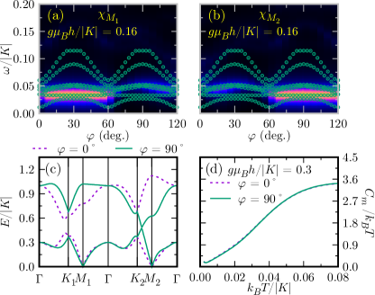
Figure 9: Dynamical spin structer factors (a) $\chi_{M_{1}}(\omega)$ and (b) $\chi_{M_{2}}(\omega)$ as a function of a field angle $\varphi$ in the $K$-$J_{3}$ model with $J_{3}/|K|=0.1$, $K<0$, and $g\mu_{B}h/|K|=0.16$. (c) Magnon dispersions and (d) magnon specific heats under both $a$- and $b$-axis fields ($\varphi=0^{\circ}$ and $\varphi=90^{\circ}$) at the critical field strength ($g\mu_{B}h/|K|=0.15$) in the $K$-$J_{3}$ model. Circle data in (a) and (b) represent the lowest seven excitation energies calculated by the thick-restarted Lanczos method Wu2000 .

The $K$-$J_{3}$ model with $K<0$ and $J_{3}>0$ has been proposed as the simplest proximate Kitaev model which shows the genuine intermediate phase under both the $a$- and $c$-axis fields BHKim2020 . We have explored the behaviors of DSSFs, magnon dispersions, and magnon specific heat of the $K$-$J_{3}$ model under in-plane magnetic fields. As shown in Fig. 9, the field-angle anisotropy in the $K$-$J_{3}$ model is less evident than those in other models. The DSSFs $\chi_{M_{1}}$, $\chi_{M_{2}}$, and $\chi_{M_{3}}$ are almost constant in the range of $0^{\circ}\leq\varphi\leq 60^{\circ}$, $60^{\circ}\leq\varphi\leq 120^{\circ}$, and $120^{\circ}\leq\varphi\leq 180^{\circ}$, respectively. The magnon bands in the polarized phase condense almost simultaneously at the three $M$ points and the field-angle anisotropy of magnon specific heat is almost suppressed.

References

- (1) A. Kitaev, Anyons in an exactly solved model and beyond, Ann. Phys. 321, 2 (2006).
- (2) Y. Kasahara, T. Ohnishi, Y. Mizukami, O. Tanaka, S. Ma, K. Sugii, N. Kurita, H. Tanaka, J. Nasu, Y. Mo tome, T. Shibauchi, and Y. Matsuda, Majorana quantization and half-integer thermal quantum Hall effect in a Kitaev spin liquid, Nature 559, 227 (2018).
- (3) T. Yokoi, S. Ma, Y. Kasahara, S. Kasahara, T. Shibauchi, N. Kurita, H. Tanaka, J. Nasu, Y. Motome, C. Hickey, S. Trebst, and Y. Matsuda, Half-integer quantized anomalous thermal Hall effect in the Kitaev material candidate -RuCl3, Science 373, 568 (2021).
- (4) K. Hwang, A. Go, J. H. Seong, T. Shibauchi, and E.-G. Moon, Identification of a Kitaev quantum spin liquid by magnetic field angle dependence, arXiv:2004.06119.
- (5) J. S. Gordon and H.-Y. Kee, Testing topological phase transitions in Kitaev materials under in-plane magnetic fields: Application to -RuCl3, Phys. Rev. Res. 3, 013179 (2021).
- (6) O. Tanaka, Y. Mizukami, R. Harasawa, K. Hashimoto, N. Kurita, H. Tanaka, S. Fujimoto, Y. Matsuda, E.-G. Moon, and T. Shibauchi, Thermodynamic evidence for field-angle dependent Majorana gap in a Kitaev spin liquid, arXiv:2007.06757.
- (7) S. M. Winter, A. A. Tsirlin, M. Daghofer, J. van den Brink, Y. Singh, P. Gegenwart, and R. Valentí, Models and materials for generalized Kitaev magnetism, J. Phys.: Condens. Matter 29, 493002 (2017).
- (8) H. Takagi, T. Takayama, G. Jackeli, G. Khaliullin, and S. E. Nagler, Concept and realization of Kitaev quantum spin liquids, Nat. Rev. Phys. 1, 264 (2019).
- (9) Y. Motome and J. Nasu, Hunting Majorana fermions in Kitaev magnets, J. Phys. Soc. Jpn. 89, 012002 (2020).
- (10) G. Jackeli and G. Khaliullin, Mott insulators in the strong spin-orbit coupling limit: From Heisenberg to a quantum compass and Kitaev models, Phys. Rev. Lett. 102, 017205 (2009).
- (11) H.-S. Kim, V. Shankar V., A. Catuneanu, and H.-Y. Kee, Kitaev magnetism in honeycomb with intermediate spin-orbit coupling, Phys. Rev. B 91, 241110(R) (2015).
- (12) J. G. Rau, E. K.-H. Lee, and H.-Y. Kee, Generic spin model for the honeycomb iridates beyond the Kitaev limit, Phys. Rev. Lett. 112, 077204 (2014).
- (13) J. A. Sears, M. Songvilay, K. W. Plumb, J. P. Clancy, Y. Qiu, Y. Zhao, D. Parshall, and Y.-J. Kim, Magnetic order in -RuCl3: A honeycomb-lattice quantum magnet with strong spin-orbit coupling, Phys. Rev. B 91, 144420 (2015).
- (14) S. M. Winter, Y. Li, H. O. Jeschke, and R. Valentí, Challenges in design of Kitaev materials: Magnetic interactions from competing energy scales, Phys. Rev. B 93, 214431 (2016).
- (15) L. J. Sandilands, Y. Tian, K. W. Plumb, Y.-J. Kim, and K. S. Burch, Scattering continuum and possible fractionalized excitations in -RuCl3, Phys. Rev. Lett. 114, 147201 (2015).
- (16) A. Banerjee, C. A. Bridges, J.-Q. Yan, A. A. Aczel, L. Li, M. B. Stone, G. E. Granroth, M. D. Lumsden, Y. Yiu, J. Knolle, S. Bhattacharjee, D. L. Kovrizhin, R. Moessner, D. A. Tennant, D. G. Mandrus, and S. E. Nagler, Proximate Kitaev quantum spin liquid behaviour in a honeycomb magnet, Nat. Mater. 15, 733 (2016).
- (17) R. Yadav, N. A. Bogdanov, V. M. Katukuri, S. Nishimoto, J. van den Brink, and L. Hozoi, Kitaev exchange and field-induced quantum spin-liquid states in honeycomb -RuCl3, Sci. Rep. 6, 37925 (2016).
- (18) A. Banerjee, J. Yan, J. Knolle, C. A. Bridges, M. B. Stone, M. D. Lumsden, D. G. Mandrus, D. A. Tennant, R. Moessner, and S. E. Nagler, Neutron scattering in the proximate quantum spin liquid -RuCl3, Science 356, 1055 (2017).
- (19) S.-H. Do, S.-Y. Park, J. Yoshitake, J. Nasu, Y. Motome, Y. Kwon, D. T. Adroja, D. J. Voneshen, K. Kim, T.-H. Jang, J.-H. Park, K.-Y. Choi, and S. Ji, Majorana fermions in the Kitaev quantum spin system -RuCl3, Nat. Phys. 13, 1079 (2017).
- (20) S. Widmann, V. Tsurkan, D. A. Prishchenko, V. G. Mazurenko, A. A. Tsirlin, and A. Loidl, Thermodynamic evidence of fractionalized excitations in -RuCl3, Phys. Rev. B 99, 094415 (2019).
- (21) Y. Kubota, H. Tanaka, T. Ono, Y. Narumi, and K. Kindo, Successive magnetic phase transitions in -RuCl3: XY-like frustrated magnet on the honeycomb lattice, Phys. Rev. B 91, 094422 (2015).
- (22) J. A. Sears, Y. Zhao, Z. Xu, J. W. Lynn, and Y.-J. Kim, Phase diagram of -RuCl3 in an in-plane magnetic field, Phys. Rev. B 95, 180411(R) (2017).
- (23) I. A. Leahy, C. A. Pocs, P. E. Siegfried, D. Graf, S.-H. Do, K.-Y. Choi, B. Normand, and M. Lee, Anomalous thermal conductivity and magnetic torque response in the honeycomb magnet -RuCl3, Phys. Rev. Lett. 118, 187203 (2017).
- (24) S.-H. Baek, S.-H. Do, K.-Y. Choi, Y. S. Kwon, A. U. B. Wolter, S. Nishimoto, J. van den Brink, and B. Büchner, Evidence for a field-induced quantum spin liquid in -RuCl3, Phys. Rev. Lett. 119, 037201 (2017).
- (25) Z. Wang, S. Reschke, D. Hüvonen, S.-H. Do, K.-Y. Choi, M. Gensch, U. Nagel, T. Rõõm, and A. Loidl, Magnetic excitations and continuum of a possibly field-induced quantum spin liquid in -RuCl3, Phys. Rev. Lett. 119, 227202 (2017).
- (26) J. Zheng, K. Ran, T. Li, J. Wang, P. Wang, B. Liu, Z.-X. Liu, B. Normand, J. Wen, and W. Yu, Gapless spin excitations in the field-induced quantum spin liquid phase of -RuCl3, Phys. Rev. Lett. 119, 227208 (2017).
- (27) A. U. B. Wolter, L. T. Corredor, L. Janssen, K. Nenkov, S. Schönecker, S.-H. Do, K.-Y. Choi, R. Albrecht, J. Hunger, T. Doert, M. Vojta, and B. Büchner, Field-induced quantum criticality in the Kitaev system -RuCl3, Phys. Rev. B 96, 041405(R) (2017).
- (28) S. M. Winter, K. Riedl, D. Kaib, R. Coldea, and R. Valentí, Probing -RuCl3 beyond magnetic order: Effects of temperature and magnetic field, Phys. Rev. Lett. 120, 077203 (2018).
- (29) A. Banerjee, P. Lampen-Kelley, J. Knolle, C. Balz, A. A. Aczel, B. Winn, Y. Liu, D. Pajerowski, J. Yan, C. A. Bridges, A. T. Savici, B. C. Chakoumakos, M. D. Lumsden, D. A. Tennant, R. Moessner, D. G. Mandrus, and S. E. Nagler, Excitations in the field-induced quantum spin liquid state of -RuCl3, npj Quantum Mater. 3, 8 (2018).
- (30) N. Jans̆a, A. Zorko, M. Gomils̆ek, M. Pregelj, K. W. Krämer, D. Biner, A. Biffin, C. Rüegg, and M. Klanjs̆ek, Observation of two types of fractional excitation in the Kitaev honeycomb magnet, Nat. Phys. 14, 786 (2018).
- (31) C. Wellm, J. Zeisner, A. Alfonsov, A. U. B. Wolter, M. Roslova, A. Isaeva, T. Doert, M. Vojta, B. Büchner, and V. Kataev, Signatures of low-energy fractionalized excitations in -RuCl3 from field-dependent microwave absorption, Phys. Rev. B 98, 184408 (2018).
- (32) C. Balz, P. Lampen-Kelley, A. Banerjee, J. Yan, Z. Lu, X. Hu, S. M. Yadav, Y. Takano, Y. Liu, D. A. Tennant, M. D. Lumsden, D. Mandrus, and S. E. Nagler, Finite field regime for a quantum spin liquid in -RuCl3, Phys. Rev. B 100, 060405(R) (2019).
- (33) J. S. Gordon, A. Catuneanu, E. S. Sørensen, and H.-Y. Kee, Theory of the field-revealed Kitaev spin liquid, Nat. Commun. 10, 2470 (2019).
- (34) H.-Y. Lee, R. Kaneko, L. E. Chern, T. Okubo, Y. Yamaji, N. Kawashima, and Y. B. Kim, Magnetic field induced quantum phases in a tensor network study of Kitaev magnets, Nat. Commun. 11, 1639 (2020).
- (35) C. Balz, L. Janssen, P. Lampen-Kelley, A. Banerjee, Y. H. Liu, J.-Q. Yan, D. G. Mandrus, M. Vojta, and S. E. Nagler, Field-induced intermediate ordered phase and anisotropic interlayer interactions in -RuCl3, Phys. Rev. B 103, 174417 (2021).
- (36) A. N. Ponomaryov, L. Zviagina, J. Wosnitza, P. Lampen-Kelley, A. Banerjee, J.-Q. Yan, C. A. Bridges, D. G. Mandrus, S. E. Nagler, and S. A. Zvyagin, Nature of magnetic excitations in the high-field phase of -RuCl3, Phys. Rev. Lett. 125, 037202 (2020).
- (37) D. Wulferding, Y. Choi, S.-H. Do, C. H. Lee, P. Lemmens, C. Faugeras, Y. Gallais, and K.-Y. Choi, Magnon bound states versus anyonic Majorana excitations in the Kitaev honeycomb magnet -RuCl3, Nat. Commun. 11, 1603 (2020).
- (38) B. H. Kim, S. Sota, T. Shirakawa, S. Yunoki, and Y.-W. Son, Proximate Kitaev system for an intermediate magnetic phase in in-plane magnetic fields, Phys. Rev. B 102, 140402(R) (2020).
- (39) M. Yamashita, J. Gouchi, Y. Uwatoko, N. Kurita, and H. Tanaka, Sample dependence of half-integer quantized thermal Hall effect in the Kitaev spin-liquid candidate -RuCl3, Phys. Rev. B 102, 220404(R) (2020).
- (40) P. Czajka, T. Gao, M. Hirschberger, P. Lampen-Kelley, A. Banerjee, J. Yan, D. G. Mandrus, S. E. Nagler, and N. P. Ong, Oscillations of the thermal conductivity in the spin-liquid state of -RuCl3, Nat. Phys. 17, 915 (2021).
- (41) S. Bachus, D. A. S. Kaib, A. Jesche, V. Tsurkan, A. Loidl, S. M. Winter, A. A. Tsirlin, R. Valentí, and P. Gegenwart, Angle-dependent thermodynamics of -RuCl3, Phys. Rev. B 103, 054440 (2021).
- (42) J. A. Sears, L. E. Chern, S. Kim, P. J. Bereciartua, S. Francoual, Y. B. Kim, and Y.-J. Kim, Ferromagnetic Kitaev interaction and the origin of large magnetic anisotropy in -RuCl3, Nat. Phys. 16, 837 (2020).
- (43) K. Ran, J. Wang, W. Wang, Z.-Y. Dong, X. Ren, S. Bao, S. Li, Z. Ma, Y. Gan, Y. Zhang, J. T. Park, G. Deng, S. Danilkin, S.-L. Yu, J.-X. Li, and J. Wen, Spin-wave excitations evidencing the Kitaev interaction in single crystalline -RuCl3, Phys. Rev. Lett. 118, 107203 (2017).
- (44) P. Laurell and S. Okamoto, Dynamical and thermal magnetic properties of the Kitaev spin liquid candidate -RuCl3, npj Quantum Mater. 5, 2 (2020).
- (45) P. A. Maksimov and A. L. Chernyshev, Rethinking -RuCl3, Phys. Rev. Res. 2, 033011 (2020).
- (46) Y. S. Hou, H. J. Xiang, and X. G. Gong, Unveiling magnetic interactions of ruthenium trichloride via constraining direction of orbital moments: Potential routes to realize a quantum spin liquid, Phys. Rev. B 96, 054410 (2017).
- (47) C. Eichstaedt, Y. Zhang, P. Laurell, S. Okamoto, A. G. Eguiluz, and T. Berlijn, Deriving models for the Kitaev spin-liquid candidate material -RuCl3 from first principles, Phys. Rev. B 100, 075110 (2019).
- (48) H. Suzuki, H. Liu, J. Bertinshaw, K. Ueda, H. Kim, S. Laha, D. Weber, Z. Yang, L. Wang, H. Takahashi, K. Fürsich, M. Minola, B. V. Lotsch, B. J. Kim, H. Yavaş, M. Daghofer, J. Chaloupka, G. Khaliullin, H. Gretarsson, and B. Keimer, Proximate ferromagnetic state in the Kitaev model material -RuCl3, Nat. Commun. 12, 4512 (2021).
- (49) K. Wu and H. Simon, Thick-restart Lanczos method for large symmetric eigenvalue problems, SIAM J. Matrix Anal. Appl. 22, 602 (2000).
- (50) J. Jaklič and P. Prelovšek, Finite-temperature properties of doped antiferromagnets, Adv. Phys. 49, 1 (2000).
- (51) M. Aichhorn, M. Daghofer, H. G. Evertz, and W. von der Linden, Low-temperature Lanczos method for strongly correlated systems, Phys. Rev. B 67, 161103(R) (2003).
- (52) L. E. Chern, E. Z. Zhang, and Y. B. Kim, Sign structure of thermal Hall conductivity and topological magnons for in-plane field polarized Kitaev magnets, Phys. Rev. Lett. 126, 147201 (2021).
- (53) A. N. Ponomaryov, E. Schulze, J. Wosnitza, P. Lampen-Kelley, A. Banerjee, J.-Q. Yan, C. A. Bridges, D. G. Mandrus, S. E. Nagler, A. K. Kolezhuk, and S. A. Zvyagin, Unconventional spin dynamics in the honeycomb-lattice material -RuCl3: High-field electron spin resonance studies, Phys. Rev. B 96, 241107(R) (2017).