Dark Energy Survey Year 3 Results: A 2.7$\%$ measurement of Baryon Acoustic Oscillation distance scale at redshift 0.835

Abstract

We present angular diameter measurements obtained by measuring the position of Baryon Acoustic Oscillations (BAO) in an optimised sample of galaxies from the first three years of Dark Energy Survey data (DES Y3). The sample consists of 7 million galaxies distributed over a footprint of 4100 deg² with $0.6<z_{\rm photo}<1.1$ and a typical redshift uncertainty of $0.03(1+z)$. The sample selection is the same as in the BAO measurement with the first year of DES data, but the analysis presented here uses three times the area, extends to higher redshift and makes a number of improvements, including a fully analytical BAO template, the use of covariances from both theory and simulations, and an extensive pre-unblinding protocol. We used two different statistics: angular correlation function and power spectrum, and validate our pipeline with an ensemble of over 1500 realistic simulations. Both statistics yield compatible results. We combine the likelihoods derived from angular correlations and spherical harmonics to constrain the ratio of comoving angular diameter distance $D_{M}$ at the effective redshift of our sample to the sound horizon scale at the drag epoch. We obtain $D_{M}(z_{\rm eff}=0.835)/r_{\rm d}=18.92\pm 0.51$, which is consistent with, but smaller than, the Planck prediction assuming flat $\Lambda$CDM, at the level of $2.3\sigma$. The analysis was performed blind and is robust to changes in a number of analysis choices. It represents the most precise BAO distance measurement from imaging data to date, and is competitive with the latest transverse ones from spectroscopic samples at $z>0.75$. When combined with DES 3x2pt + SNIa, they lead to improvements in $H_{0}$ and $\Omega_{m}$ constraints by $\sim 20\%$.

I Introduction

The scientific knowledge of the Universe changed in the 1990s with the discovery of its accelerated expansion (Riess et al., 1998; Perlmutter et al., 1999). This remarkable discovery opened the door to the current cosmological standard model, $\Lambda$CDM. The model is very well established, since it is based on a very large set of independent observations that it can explain with high accuracy. However, it has shocking consequences. Only a small fraction (around 5%) of the content of our Universe is ordinary matter. The other 95% is composed of exotic entities called dark matter and dark energy, that have not been detected yet in laboratories. $\Lambda$CDM describes the dominant component of the matter-energy content of the Universe, dark energy, as a cosmological constant $\Lambda$, a description that is in agreement with all the current cosmological observations (Particle Data Group et al., 2020). However, the value of $\Lambda$ itself is not compatible with the Standard Model of particle physics (Weinberg, 1989; Padmanabhan, 2003). The current measurements of dark energy properties are not yet precise enough to distinguish between possible explanations, like the incompleteness of General Relativity to describe gravity at cosmological scales or the existence of some mysterious fluid with negative pressure filling the whole Universe, are still possible.

Several observational probes are used to study the nature of dark energy. Among them, the measurement of the evolution with redshift of the angular diameter distance and the Hubble distance, using the scale of the Baryon Acoustic Oscillations (BAO) as a standard ruler, is one of the most robust, since it is insensitive to systematic uncertainties related to the astrophysical properties of the tracers (galaxies, quasars or the Lyman-$\alpha$ forest). In addition, the physics that causes BAO is well understood, which allows very precise measurements with the current cosmological surveys. The BAO signal was first detected in 2005 by both the Sloan Digital Sky Survey (SDSS) (Eisenstein et al., 2005) and the 2-degree Field Galaxy Redshift Survey (2dFGRS) (Percival et al., 2001; Cole et al., 2005). Today there are many detections at different redshifts from SDSS I, II, III and IV (Percival et al., 2007; Gaztañaga et al., 2009; Percival et al., 2010; Ross et al., 2015; Alam et al., 2017; Ata et al., 2018; Busca et al., 2013; Slosar et al., 2013; Font-Ribera et al., 2014; Delubac et al., 2015; Bautista et al., 2017; du Mas des Bourboux et al., 2020; Alam et al., 2021), the 6-degree Field Galaxy Survey (6dFGS) (Beutler et al., 2011) and WiggleZ (Blake et al., 2011a, b; Kazin et al., 2014; Hinton et al., 2017), mapping the redshift evolution of the angular diameter distance.

The Dark Energy Survey (DES, Flaugher (2005); Dark Energy Survey Collaboration et al. (2016)) is a photometric galaxy survey that probes the physical nature of dark energy by means of several independent and complementary probes. One of these probes is the precise study of the spatial distribution of galaxies, and in particular, the BAO standard ruler. Since DES is a photometric survey, its precision in the measurement of redshifts is limited. However, a precise determination of the evolution of the angular distance with redshift is possible through the measurement of angular correlation functions or angular power spectra, as was already probed with the DES Y1 data (Dark Energy Survey Collaboration et al., 2019). Other measurements of the BAO signal in various photometric data samples have been presented in Refs. Padmanabhan et al. (2007); Estrada et al. (2009); Hütsi (2010); Sánchez et al. (2011); Crocce et al. (2011a); Seo et al. (2012); Carnero et al. (2012) using a variety of methodologies.

In this paper, a new determination of the BAO scale is presented. The measurement uses the imaging data from DES Y3, described in Sevilla-Noarbe et al. (2021), to measure the angular diameter distance to red galaxies that have been specially selected (Carnero Rosell et al., 2021) with photometric redshifts $0.6<z_{\rm photo}<1.1$. DES has imaged a 5,000 deg² footprint of the Southern hemisphere using five passbands, $grizY$, collecting the properties of over 300 million galaxies. Here, we use 7 million galaxies over 4100 deg², that were color and magnitude selected to balance trade-offs in BAO measurements between the redshift precision and the number density. We use these data, supported by 1952 mock realizations of our sample, to measure the BAO scale at an effective redshift of $0.835$.

The measurement we present is supported by a series of companion papers. In Carnero Rosell et al. (2021) we present all the details of the selection of the galaxy sample, that was optimised for $z>0.6$ BAO measurements, the tests of its basic properties, the mitigation of observational systematic effects and the photometric redshift validations, extending what was done in Crocce et al. (2019). In Ferrero et al. (2021) we describe the mock catalogues we have developed to test the measurement methods. These mocks match the spatial properties of the data sample and the photo-$z$ resolution.

The structure of this paper is as follows. Section II summarizes the data we used, including all of its basic properties and the process we used to mitigate systematic effects. Section III presents the different sets of simulations used to validate the analysis. Section IV describes the analysis methodology, including the techniques to measure the clustering of galaxies (both angular correlation function and angular power spectrum), the estimation of the covariance matrices and the production of the templates that have been used to fit the BAO scale. In addition, it also presents how the BAO scale is extracted from the data. Section V present the validation of the entire analysis using simulations. Section VI describes the full set of pre-unblinding tests that we defined as a requirement to be passed before revealing the final results. Section VII presents our results, starting with the clustering measurements and the resulting BAO scale followed by the distance measurement derived from this scale. Finally, Section VIII is devoted to the cosmological implications of this measurement, including a comparison to predictions of the flat $\Lambda$CDM model and other BAO scale distance measurements. Our conclusions are presented in Section IX.

The fiducial cosmology we use to quote our primary results is a flat $\Lambda$CDM model with $\Omega_{m}=0.31$, $h=0.676$, $n_{s}=0.97$ and $\sigma_{8}=0.83$; consistent with Planck Collaboration et al. (2020) (we denote this as Planck hereafter). However our mocks, and therefore all the statistical and systematics tests to validate our methodology, were carried out using $\Omega_{m}=0.25$ and $h=0.7$ (denoted as MICE in what follows). This cosmology matches the one of the MICE N-Body simulations Fosalba et al. (2015a); Crocce et al. (2015); Fosalba et al. (2015b), which was used to calibrate the mock galaxy samples themselves. We demonstrate that our results are not sensitive to this choice.

It is important to remark that the whole analysis was performed blinded. The sample selection cuts and the estimation of photometric redshifts and redshift distributions, the treatment of observational systematics, and the analysis choices were defined and completed a priori. In addition, a detailed set of tests to be passed before unblinding the results was put in place. Only when the analysis passed this predefined criteria, we unblinded the measurement of the BAO scale.

II Dark Energy Survey Data

II.1 DES Y3-GOLD catalogue

The Dark Energy Survey (DES) observed for six years using the Dark Energy Camera (DECam Flaugher et al. (2015)) at the Blanco 4m telescope at the Cerro Tololo Inter-American Observatory (CTIO) in Chile. The survey covered 5000 sq. deg. in $grizY$ bandpasses to approximately 10 overlapping dithered exposures in each filter. We utilize data taken during the first three years of DES operations (DES Y3), which made up DES Data Release 1 (DR1 Dark Energy Survey Collaboration et al. (2018)). This analysis covers the full 5000 sq. deg. survey footprint for the first time, but at approximately half the full-survey depth. The data is processed, calibrated, and coadded to produce a photometric data set of 390 million objects that is further refined to a ‘Gold’ sample for cosmological use Sevilla-Noarbe et al. (2021). The Y3 GOLD sample includes cuts on minimal image depth and quality, additional calibration and deblending, and quality flags to identify problematic photometry and regions of the sky with substantial photometric degradation (e.g., around bright stars). The Y3 GOLD sample extends to a 10$\sigma$ limiting magnitude of 23 in $i$-band and it is the basis for the definition of the BAO sample.

II.2 BAO Sample

We select a subsample of red galaxies from the Y3 GOLD sample Sevilla-Noarbe et al. (2021) following the same color selection as in Y1 (Crocce et al., 2019), designed to balance the sample density with the photo-$z$ precision above redshifts greater than $0.5$. The sample covers 4108.47 ${\rm deg}^{2}$, almost three times larger than the Y1 BAO sample, and comprises $7,031,993$ galaxies in the redshift range $0.6<z<1.1$, up to a magnitude limit of $i<22.3\ (AB,10\sigma$). Full details about the sample selection and characterization is found in Carnero Rosell et al. (2021), here we summarize the main properties.

Improvements in data reduction and processing between Y1 and Y3 increased the DES detection efficiency, which translated into a higher number density of sources, even though the number of exposures per pointing in the footprint is in average the same. We take full advantage of this optimization for the BAO sample and extend the analysis from $z_{\rm photo}=1$ to $z_{\rm photo}=1.1$ and to a fainter magnitude limit with respect to Y1 (22.3 instead of 22, in the $i$-band). Our forecasts showed that this extension of the sample meant a $10\%$ gain in the precision of the combined BAO distance measurement.

During the selection process we used ngmix SOF magnitudes (hereafter referred to as SOF) with chromatic corrections and dereddened using SED-dependent extinction corrections. These magnitudes are defined in Sevilla-Noarbe et al. (2021). We also use the morphological classification based on SOF photometry to select secure galaxies. These choices are common to all DES Y3 cosmological results.

We start by applying the same color cut as in Y1 to the Gold sample to select red galaxies. Despite the changes in photometry from Y1 and Y3, the color selection still isolates galaxies at $z>0.5$, as attested in (Carnero Rosell et al., 2021). The primary selection includes the aforementioned color cut, a magnitude cut as a function of photometric redshift $z_{\rm photo}$ (to remove fainter galaxies at lower redshifts) and the redshift range. The cuts applied are:

$$(i_{\texttt{{SOF}}}-z_{\texttt{{SOF}}})+2.0(r_{\texttt{{SOF}}}-i_{\texttt{{SOF}}})>1.7,$$ (1)

$$i_{\texttt{{SOF}}}<19+3.0\,z_{\rm photo},$$ (2)

$$0.6<z_{\rm photo}<1.1,$$ (3)

where $z_{\rm photo}$ is the photometric redshift estimate, which we describe in detail in Sec. II.3. In addition we impose a bright magnitude cut $17.5<i_{\texttt{{SOF}}}$ to remove bright contaminant objects such as binary stars. Stellar contamination is mitigated with the galaxy and star classifier EXTENDED_CLASS_MASH_SOF from the Y3 GOLD catalogue. Likewise, we remove sources that are flagged as suspicious or with corrupted photometry (see Carnero Rosell et al. (2021)).

A summary of the BAO sample properties is given in Table LABEL:tab:sample, and an in-depth discussion of the selection process and flags can be found in Carnero Rosell et al. (2021).

Table 1: Main properties of the BAO sample as a function of tomographic bin: mean redshift, number of galaxies, mean photo-$z$ accuracy (in units of $(1+z)$) and $68\%$ width of the true redshift distribution estimates, see Sec. II.3. The latter are found by stacking spectroscopic redshifts from a matched sample with the VIPERS dataset. The sample covers 4108.47 deg². Full details can be found in Carnero Rosell et al. (2021).

$z_{\rm photo}$	$\bar{z}$	$N_{\rm gal}$	$\sigma_{68}$	$W_{68}$
$0.6<z<0.7$	0.65	1478178	0.021	0.045
$0.7<z<0.8$	0.74	1632805	0.025	0.052
$0.8<z<0.9$	0.84	1727646	0.029	0.063
$0.9<z<1.0$	0.93	1315604	0.030	0.063
$1.0<z<1.1$	1.02	877760	0.040	0.081

II.3 Photometric Redshifts

We measure the BAO scale in tomographic redshift bins of width $\Delta z=0.1$ from $0.6$ to $1.1$. In order to assign galaxies to each redshift bin we use the photo-$z$ estimate given by the Directional Neighborhood Fitting (DNF) algorithm De Vicente et al. (2016), which was trained using SOF $griz$ fluxes on a large training sample. In this work, this reference dataset includes $\sim 2.2\times 10^{5}$ spectra matched to DES objects from 24 different spectroscopic catalogues, in particular SDSS DR14 SDSS Collaboration, (2018) and the OzDES program Childress et al. (2017). DNF performs a nearest-neighbors fit to the hyper-plane in color and magnitude space to this training set, and predicts the best photo-$z$ estimate (called Z_MEAN in the DES catalogues), as well as the redshift of the closest neighbor (Z_MC) and the full PDF distribution. We use Z_MEAN to assign galaxies to each tomographic bin.

In order to estimate the true redshift distribution $n(z)$ in each tomographic bin we construct a matched sample Carnero Rosell et al. (2021), within one arcsec apertures, with the second public data release (PDR2) Scodeggio et al. (2018) from “VIMOS Public Extragalactic Redshift Survey” (VIPERS) Guzzo et al. (2014). VIPERS was designed to be a complete galaxy sample up to $i<22.5$ for redshifts above $0.5$ and covers $16.32$ deg² in the DES footprint, containing 74591 BAO sample galaxies in the matched catalogue. Each of these galaxies is weighted to account for target selection, colour selection and spectroscopic efficiency. We stack the spectroscopic redshifts $z_{\rm VIPERS}$ from the matched catalogue to estimate our five $n(z)$’s. In Carnero Rosell et al. (2021) we also use the stacking of the DNF Z_MC or DNF PDF’s to validate the redshift distributions of the BAO sample.

Table LABEL:tab:sample contains estimates of the photometric redshift accuracy per galaxy, $\sigma_{68}$, defined as the half width of the interval containing the median $68\%$ of values in the distribution of $(\texttt{\small Z\_MEAN}-z_{\rm VIPERS})/(1+z_{\rm VIPERS})$. It also shows an estimate of the width of the individual $n(z)$’s, $W_{68}$, similarly defined as the $68\%$ confidence region of the stacking of $z_{\rm VIPERS}$. It also contains the mean of each $n(z)$, $\bar{z}$, that matches well the geometric mean of the corresponding bin edges, except at the last bin where the distribution is a bit skewed towards low redshifts.

II.4 Angular Mask

The BAO sample footprint is constructed directly from the high resolution HEALPix Górski et al. (2005) maps given in Sevilla-Noarbe et al. (2021). The main requirements imposed in the footprint are: Each pixel has to be observed at least once in $griz$, with a coverage greater than $80\%$. Pixels affected by foreground sources like extended galaxies or bright stars and regions affected by image artifacts are removed. Pixels with 10-$\sigma$ limited depth of $i_{\texttt{{SOF}},{\rm lim}}<22.3$ are removed, consistent with the faintest magnitudes in the BAO sample, see Eqs.(2,3). Pixels with a 10-$\sigma$ magnitude limit in $r_{\texttt{{SOF}}}$ and $z_{\texttt{{SOF}}}$ bands such that $2\,r_{\texttt{{SOF}},{\rm lim}}-z_{\texttt{{SOF}},{\rm lim}}<24$ are also removed, in order to ensure reliable measurements of the color defined in Eq. (1). The area of the BAO sample covers the 4108.47 deg² and is shown in Fig. 1 as a projected density field.

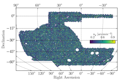
Figure 1: BAO sample projected density field. The effective area is 4108.47 deg²

II.5 Observational Systematics

The observed number of galaxies is expected to have a non-trivial selection function that depends on various observing conditions of the survey, in addition to external conditions such as dust extinction or the dependence of stellar density with galactic latitude. These properties, which are themselves correlated, vary spatially and in general will have large-scale modes. This imprints a bias in the clustering signal if not accounted for Ross et al. (2011); Leistedt and Peiris (2014); Ross et al. (2017); Laurent et al. (2017); Bautista et al. (2018); Icaza-Lizaola et al. (2020); Vakili et al. (2020); Weaverdyck and Huterer (2021). We correct this effect by applying weights to each galaxy corresponding to the inverse of the estimated angular selection function. This methodology, while now more widely adopted in the literature, was first applied in DES for the lens sample used in the DES Y1 3x2pt analysis in Elvin-Poole et al. (2018). In Y3, the same methodology is applied to all clustering samples. Details about the method and results for other Y3 samples are given in Rodríguez-Monroy et al. (2021) and for the BAO sample in Carnero Rosell et al. (2021).

The method consists on assigning weights to correct for the spurious clustering signal from individual survey properties, iteratively in order of decreasing significance until a global threshold is met. In the Y3 GOLD catalogue, more than 100 survey property maps are available. However the majority of these maps are highly correlated among themselves. First we use a criterion to eliminate the highest correlations based on their Pearson’s correlation coefficient matrix. This reduces the list of maps to a subset of 26 maps, including depth, airmass, stellar density and E(B-V) extinction (see Appendix B of Carnero Rosell et al. (2021)). We start by measuring the galaxy density as a function of survey property, for each tomographic bin separately. We use a set of 1000 lognormal realisations to measure what this relation is expected to look like in the absence of any induced systematic, and hence to estimate the significance of the relation found on the data. We then assign position-dependent weights to galaxies to remove the most significant trend in question. All weights are assigned with a linear fit to the density-observing condition relation, and we find no evidence for requiring additional terms in the model. This process is run iteratively until all density-observing conditions relations are below a given threshold. In the case of the BAO sample, we chose the threshold to be equivalent to $<99\%$ of mock values.

Contrary to Y1, in Y3 we find that the observational systematic correction is several times the statistical error, mostly due to the increase in sample size. During the blinded period we tested variations in the treatment of systematics, e.g. masking regions with extreme survey property values or varying the significance threshold. They all led to consistent final weights maps. Moreover by comparison to a set of 1000 lognormal mocks, we find that the systematic error on the correction from over-fitting was small compared with the statistical errors in the angular correlation function or angular power spectrum itself. In Sec. VII.3 we show that the recovered BAO distance measurement is insensitive of the observational weights. More details about the mitigation of systematics can be found in Carnero Rosell et al. (2021).

III Simulations

In what follows, we discuss the two sets of mock galaxy catalogues that we use throughout the analysis to validate the whole BAO distance measurement.

III.1 ICE-COLA (quasi-n-body) Mocks

We create a set of 1952 mock catalogues of the DES Y3 BAO sample that reproduce with high accuracy the principal properties of the data: (i) the sample observational volume, (ii) the abundance of galaxies, true redshift distribution and photometric redshift uncertainty and (iii) the clustering as a function of redshift. We refer the reader to Ferrero et al. (2021) for further details, and highlight here only the basic features of the ICE-COLA mocks used for this work.

This set of mocks is obtained using $N_{\rm sim}=488$ fast quasi-$N$-body simulations generated with the ICE-COLA code (Izard, Crocce, and Fosalba, 2016). The COLA method (Tassev et al., 2013; Koda et al., 2016) uses second order Lagrangian Perturbation Theory (2LPT) combined with a Particle-Mesh (PM) gravity solver. The latter is used to solve particle trajectories on small scales, where the 2LPT accuracy is lower compared to the full $N$-body solution. The ICE-COLA algorithm extends the COLA algorithm to produce on-the-fly light-cone halo catalogues and weak lensing maps. The simulations use $2048^{3}$ particles in a box of size of $1536$ Mpc $h^{-1}$, matching the mass resolution and 1/8 of the volume of the MICE Grand Challenge simulation (Fosalba et al., 2015a; Crocce et al., 2015). A total of 64 box replications (four boxes in each Cartesian direction) are needed to create a full sky light-cone up to redshift $\sim 1.43$.

Mocks of galaxies are created populating halos following the recipe of a hybrid Halo Occupation Distribution and Halo Abundance Matching model Carretero et al. (2015); Avila et al. (2018). The algorithm has two free parameters per tomographic bin, setting the satellite number and the total number of galaxies as a function of host halo mass. These total of ten free parameters are found by running an automatic likelihood minimization. This automatic calibration received as inputs the redshift distribution, $n(z)$, and the unblinded data measurements of angular clustering $w(\theta)$ at scales smaller than 1 deg. Another important property that needs to be covered by the mocks is a realistic photometric redshift distribution. In contrast to the data, for the simulated halos we have the true redshifts and the photometric ones need to be derived. This is done by using the 2D probability distribution $P(z_{\rm ph},z_{\rm sp})$ of galaxies present in both VIPERS and DES Y3 data sets. Finally, four non-overlapping DES Y3 footprint masks are placed on each full-sky halo catalogue allowing to have 4 times more galaxy mocks than the total number of full-sky simulations.

The replications mentioned above introduce strong correlations among the measured $w(\theta)$ of tomographic bins that are not adjacent. This is discussed more in detail in Ferrero et al. (2021) where it is shown that up to a $\sim 10$% of the particles are repeated (depending on the tomographic bin combination) once we impose the DES Y3 footprint and $n(z)$. This leads to non-zero covariances for tomographic bins that have no redshift overlap otherwise. For this reason we avoid using the ICE-COLA mocks as one of our primary covariance estimation tools, but use them only to validate and benchmark the process of angular diameter distance measurements.

III.2 FLASK (lognormal) Mocks

Lognormal distributions have been shown to be a very good approximation to cosmological fields (Coles and Jones (1991); Clerkin et al. (2017)). For some applications, they are a very useful tool due to their flexibility and for being much less computationally expensive than full N-body simulation runs.

We produce a set of lognormal mock catalogs using the publicly available code Full sky Lognormal Astro fields Simulation Kit (FLASK) Xavier et al. (2016). FLASK is able to quickly generate random catalog realisations, in tomographic bins, with the same statistical properties of the DES Y3 BAO galaxy sample.

We generate 2000 mock galaxy position catalogs and density maps with the DES Y3 footprint in HEALPix resolution NSIDE = 4096. We use as simulation input the galaxy bias and number density per tomographic bin, the full set of auto and cross correlations, and the lognormal field shift parameters per bin, as defined in Xavier et al. (2016); Friedrich et al. (2020). The set of input correlations are the mean values measured in the ICE-COLA mocks. The galaxy biases used in the FLASK simulations are, namely, $b=[1.576,1.595,1.694,1.821,2.033]$ for the respective five redshift bins (also extracted from the ICE-COLA mocks). The cosmology adopted for FLASK is the MICE cosmology. Considering this cosmology and the $n(z)$ of sample, the lognormal shift parameters for the five tomographic bins are [0.600, 0.595, 0.593, 0.572, 0.580], respectively.

For the angular power spectrum estimates, we convert the FLASK catalogs to HEALPix maps with NSIDE=1024, and then measure the auto and cross spectra using the NaMaster code Alonso et al. (2019), with the same specifications as with the real data (see Sec. IV.1). In real space, the auto and cross correlations of each of the 2000 catalogs were measured using TreeCorr Jarvis et al. (2004). We set the bin_slop parameter as $bs=0.0$ which means a brute force computation of the 2-point estimators.

We use these measurements to validate our baseline covariance based on the code CosmoLike Krause and Eifler (2017) (see Sec. IV.3).

IV Analysis

IV.1 Clustering Measurements

We measure the clustering signal on the BAO sample using three different statistics, the angular correlation function $w(\theta)$ (ACF), the angular power spectrum in spherical harmonics, $C_{\ell}$ (APS) and the three-dimensional correlation in terms of projected comoving separation $\xi_{p}(s_{\perp})$.

IV.1.1 Angular correlation function: $w(\theta)$

The angular correlation function is computed after creating a uniform random sample within the mask defined in Sec. (II.4) with a size of 20 times that of the data sample in each tomographic bin. As pointed out in Sec. II.4 the mask has a pixel resolution of 4096 but includes a fractional coverage per pixel. We downsample the randoms according to this coverage and keep only pixels with coverage equal or larger than $80\%$. Given the random sample, we use the well known Landy-Szalay estimator Landy and Szalay (1993)

$$w(\theta)=\frac{DD(\theta)-2DR(\theta)+RR(\theta)}{RR(\theta)},$$ (4)

where $DD$, $DR$ and $RR$ being the normalised counts of data-data, data-random and random-random pairs, with angular separation $\theta\pm\Delta\theta/2$, with $\Delta\theta$ being the bin size, and all pair-counts are normalized based on the total size of each sample. We bin pair-counts at a bin size of 0.05 degrees but later combined these into larger bin sizes to explore the dependence of the BAO fit statistics on angular resolution or size of the covariance matrix. As we will see (e.g. Figure 4), the BAO feature appears at $\sim$2.5 to $\sim$3.5 degrees at the redshift range considered here and has a width of approximately 1 degree. Hence, any coarse-graining due to this primary binning is not expected to affect the BAO measurements. We compute the clustering using two different pair counting codes, TreeCorr Jarvis et al. (2004) and CUTE Alonso (2012), performing an extensive code-comparison to ensure consistent results. Finding excellent agreement between codes, we use CUTE with the brute force configuration as the default clustering code for the rest of the analysis. After the tests in section V we adopted a fiducial bin-size of $\Delta\theta=0.2\deg$, $\theta_{\rm min}=0.5\deg$ and $\theta_{\rm max}=5\deg$, which yields $N=22$ angular bins in total.

IV.1.2 Angular power spectrum: $C_{\ell}$

We measure the angular power spectrum of galaxies using the so-called “Pseudo-$C_{\ell}$” (PCL) estimator (Hivon et al., 2002) as implemented in the NaMASTER code (Alonso et al., 2019). For constructing galaxy overdensity maps, we use the HEALPix equal-area pixelization scheme, with a resolution of ${\rm NSIDE}=1024$, corresponding to a mean spacing of $\sim 0.06$ degrees. The equal-area pixelization allows computing the galaxy overdensity as $\delta_{g}=(N_{p}/w_{p})(\sum_{p}w_{p}/\sum_{p}N_{p})-1$ where $N_{p}$ is the number of galaxies in pixel $p$ and $w_{p}$ the pixelized mask, that gives the fraction of the area of pixel $p$ covered by the survey.

The discrete nature of galaxy number counts introduces a noise contribution to the estimated power spectrum, also known as noise-bias. We assume this noise to be Poissonian, estimate it analytically following (Alonso et al., 2019; Nicola et al., 2020), and subtract it from our power spectrum estimates. Deviations from the Poissonian approximation are expected to be captured by broad-band terms in our template.

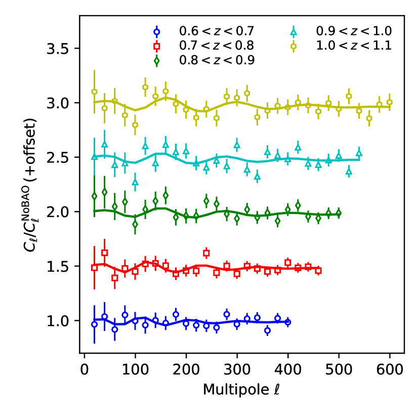
Figure 5: The isolated measured BAO feature, same as Figure 4, but in harmonic space, using the angular power spectrum, $C_{\ell}$. Vertical offsets of +0.5 have been sequentially added with each tomographic bin. The BAO feature stretches to larger values of $\ell$ with increasing redshift, as it has the same co-moving scale. The error bars are based on the fiducial Planck covariance. The solid lines represent the best fit.

We bin the angular power spectrum estimates into bandpowers, assuming equal weight for all modes. We use piecewise-linear, contiguous bins starting at a minimal multipole of $\ell_{\rm min}=10$ up to $\ell=1000$ and different values of $\Delta\ell$, chosen to guarantee a good signal-to-noise ratio across the bandpowers and remain flexible for scale cuts. After the tests in section V, we adopted as fiducial choices $\ell_{\rm min}=10$, $\Delta\ell=20$ and an $\ell_{\rm max}$ scale-cut approximately corresponding to a $k_{\rm max}=0.25h\,{\rm Mpc}^{-1}$ under the Limber relation, $k_{\rm max}=\ell_{\rm max}/r(\bar{z})$, evaluated at the mean redshift of each tomographic bin and the fiducial cosmology of our analysis. This $\ell$-binning allows us to resolve a BAO cycle with approximately 7 points (see Figure 5). When constructing the likelihood, we consider the effect of bandpower binning on the theory predictions using bandpower windows that account, in that order, for the effect of mode-coupling, binning averaging, and decoupling, following Sec 2.1.3 of Alonso et al. (2019).

IV.1.3 Projected Clustering: $\xi_{p}(s_{\perp})$

In spectroscopic surveys, it is a common practice to transform redshifts to distances in order to measure physical comoving distances between galaxies. This enables access to three-dimensional information and measurements of the BAO shift parameter along and across the line-of-sight.

Ross et al. (2017) showed that for photometric surveys, whereas the radial clustering signal is erased due to the redshift uncertainty, angular BAO information remains intact albeit smeared in the radial direction. That paper also showed that for a DES-like BAO sample representing the two-point correlation function as a function of the apparent perpendicular comoving distance ($s_{\perp}$), for different orientations with respect to the line-of-sight ($\mu$), leads to a BAO position that aligns very well as a function of $\mu$. Hence, following Ross et al. (2017), we measure the anisotropic clustering $\xi(s_{\perp},s_{\parallel})$ using the Landy-Szalay estimator Landy and Szalay (1993):

$$\xi(s_{\perp},s_{\parallel})=\frac{DD(s_{\perp},s_{\parallel})-2\cdot DR(s_{\perp},s_{\parallel})+RR(s_{\perp},s_{\parallel})}{RR(s_{\perp},s_{\parallel})}$$ (5)

with the normalised pair-counts separated by $s_{\parallel}$ and $s_{\perp}$ along and across the line-of-sight, respectively. We remark that distances $s_{\perp}$ and $s_{\parallel}$ are obtained by transforming photometric redshift and angular positions to comoving positions using the MICE fiducial cosmology. Given the aforementioned alignment of BAO, we can combine our measurements into

$$\xi_{p}({s_{\perp})=\int_{0}^{1}w(\mu)\xi\big{(}s_{\perp}(s,\mu),s_{\parallel}(s,\mu)\big{)}\ d\mu}\,,$$ (6)

where $w(\mu)$ would a priori be an inverse variance weighting. Ref. Ross et al. (2017) found that for $\mu<0.8$ and $\sigma_{z}\geq 0.02(1+z)$, our typical photo-$z$ error, the BAO signal is at a nearly constant $s_{\perp}$ while the signal for $\mu>0.8$ is greatly diminished. Hence, for simplicity, one can approximate $w$ by

$$w(\mu)=\begin{cases}\frac{1}{0.8}&\mu\leq 0.8\\ 0&\mu>0.8.\\ \end{cases}$$ (7)

Additionally, we could add a redshift-dependent FKP-like ((Feldman et al., 1994)) weight including the redshift uncertainty (Eq. (16) of Ross et al. (2017)). This per-galaxy weight is used to account for the change of BAO signal-to-noise ratio with redshift. We estimated it to be relatively flat, and we neglect it for the measurements shown here.

This estimator has the advantage that all the galaxies in the full redshift range $0.6<z_{\rm ph}<1.1$ can be combined into a single clustering measurement with the full accumulated BAO signal, as opposed to splitting them into redshift bins. Ross et al. (2017) showed that this estimator could reduce the statistical uncertainty with respect to using the angular correlation function. However, we found in Dark Energy Survey Collaboration et al. (2019) that the modelling was slightly less robust and argued that this could be due to the Gaussian assumption for the redshift uncertainties. For this reason this was not included in the fiducial analysis for Y1 and for this work. We only include it in this study for visual purposes. After the completion of this work, we have submitted a new study to improve the modelling of $\xi_{p}$ Chan et al. (2021) that may be applied in follow-up works to the DES data.

For this estimator, we perform pair-counts with $\Delta s_{\perp}=5{\rm Mpc}/h$, $\Delta s_{\parallel}=1{\rm Mpc}/h$, $s_{\perp,{\rm max}}=175{\rm Mpc}/h$, $s_{\parallel,{\rm max}}=120{\rm Mpc}/h$. With the fine binning in $s_{\parallel}$ being necessary to integrate $\mu$ in Equation 6 and the maximum sizes set to avoid excessive computing resources. The $\Delta s_{\perp}=5{\rm Mpc}/h$ choice is relatively standard for $\xi(r)$ analysis. Nevertheless, we remark that no BAO fits are derived in this paper from this estimator and we refer to the follow-up work on this estimator for further details and analysis choices Chan et al. (2021).

IV.2 BAO Template

We extract the BAO distance measurement from the clustering signal using a template-based method. This approach has been extensively used in the literature, mostly for spectroscopic datasets but also for photometric ones (e.g. Chan et al. (2018)). The main difference for the latter case is that one can extract mainly the angular diameter distance.

The main difference with previous template based BAO analysis, and in particular our DES Y1 results, is that our template is now fully obtained from first principles, including the damping of the BAO features. We implement this by means of the resummation of infrared (long wavelength) modes put forward in Senatore and Zaldarriaga (2015); Blas et al. (2016) and others. This replaces the previous methodology of calibrating the BAO damping to be used in the data with mock simulations, and enable us to easily change the template for different cosmologies. We build a template for both the configuration space and harmonic space analysis.

We build the BAO template starting from a linear power spectrum $P_{\rm lin}(k)$ obtained with Camb (Lewis et al., 2000). At BAO scales the main modification due to non-linear evolution is the broadening of the BAO feature due to large-scale flows. We model this by introducing a Gaussian damping of the BAO wiggles, after isolating this component from the full power spectrum shape:

$$P(k,\mu)=(b+\mu^{2}f)^{2}\left[(P_{\rm lin}-P_{\rm nw})e^{-k^{2}\Sigma_{\rm tot}^{2}}+P_{\rm nw}\right],$$ (8)

where $P_{\rm nw}$ describes the smooth shape of the power spectrum and all the BAO information is in $P_{\rm lin}-P_{\rm nw}$. In Eq. (8), $\mu\equiv{\rm cos}(\theta_{\rm LOS})$ = $k_{||}/k$, $b$ is the linear galaxy bias and $f$ is the logarithmic derivative of the growth factor with respect to the scale factor (at the given cosmology) evaluated at the effective redshift of the sample. The pre-factor in Eq. (8) accounts for linear-theory redshift space distortions (Kaiser, 1987). The bias parameters $b$ are obtained by fitting to $w(\theta)$ measurement from the data at three linear bins between 0.5 and 1 degree (see details in Ferrero et al., 2021). Note that these scales do not contain any BAO information, hence these measurements do not interfere with the blinding scheme. We also note that the non-linearities at small scales are expected to only appear below 0.3 deg., see Krause et al. (2021).

There are several methods to define the smooth “no-wiggle” power spectrum, $P_{\rm nw}(k)$. We follow the 1D Gaussian smoothing in log-space described in Appendix A of Vlah et al. (2016). We start by defining the ratio of $P$ and a smooth approximation to it, for which we employed the no-wiggle fitting formulae from Eisenstein and Hu (1998) (hereafter EH). This reduces the dynamical range and makes the filtering more efficient. Then

$$P_{\rm nw}(k)=P_{\rm EH}(k)\times\left[{\mathcal{F}}*R\right](k)$$ (9)

where $R(k)=P(k)/P_{\rm EH}$ and the convolution with the filter ${\mathcal{F}}$ is in log₁₀ variables,

$$\left[{\mathcal{F}}*R\right](k)=\frac{1}{\sqrt{2\pi}\lambda}\int d\log qR(q)\exp\left[-(\log(k/q))^{2}/2\lambda^{2}\right].$$

We use $\lambda=0.25$, a standard value for which we recover $P_{\rm nw}\rightarrow P_{\rm lin}$ at low and large $k$.

For the resummation of infrared modes, leading to the Gaussian damping of the BAO feature in Eq. (8), we take as a reference the implementation in Ivanov et al. (2020); Ivanov and Sibiryakov (2018) and write,

$$\Sigma^{2}_{\rm tot}(\mu)=\mu^{2}\Sigma_{\parallel}^{2}+(1-\mu^{2})\Sigma_{\perp}^{2}+f\mu^{2}(\mu^{2}-1)\delta\Sigma^{2}$$ (10)

where $\Sigma_{\parallel}=(1+f)\Sigma$ and $\Sigma_{\perp}=\Sigma$, with

$$\Sigma^{2} = \frac{1}{6\pi^{2}}\int_{0}^{k_{s}}dq\,P_{\rm nw}(q)\left[1-j_{0}(q\ell_{\rm BAO})+2j_{2}(q\ell_{\rm BAO})\right]\,$$

$$\delta\Sigma^{2} = \frac{1}{2\pi^{2}}\int_{0}^{k_{s}}dq\,P_{\rm nw}(q)j_{2}(q\ell_{\rm BAO})$$ (11)

where $j_{n}$ are the spherical Bessel functions of order $n$, while $\ell_{\rm BAO}$ is the correlation length of BAO. As a reference we choose values $k_{s}=0.2\,{\it h}\,{\rm Mpc}^{-1}$ and $\ell_{\rm BAO}=110\,{\it h}^{-1}\,{\rm Mpc}$, but our results do not depend on these choices. We assume a damping that scales with the growth factor: $\Sigma=\Sigma_{0}\cdot D(z)$ and $\delta\Sigma=\delta\Sigma_{0}\cdot D(z)$. For the MICE cosmology we obtain $\Sigma_{0}=5.80\,{\it h}^{-1}\,{\rm Mpc}$ and $\delta\Sigma_{0}=3.18\,{\it h}^{-1}\,{\rm Mpc}$ while for the Planck cosmology we find $\Sigma_{0}=5.30\,{\it h}^{-1}\,{\rm Mpc}$ and $\delta\Sigma_{0}=2.81\,{\it h}^{-1}\,{\rm Mpc}$.

As in Chan et al. (2018), we have also determined $\Sigma$ (i.e. $\Sigma_{\rm tot}$ from Eq. (10) without the $\delta\Sigma$ term) directly by fitting to the mean of the COLA mocks using different values of $\Sigma$. The best fit (minimum $\chi^{2}$) $\Sigma$ is $5.85\,{\it h}^{-1}\,{\rm Mpc}$ and it is fully consistent with the analytical MICE cosmology result from Eq. (10).

Once provided with $P(k,\mu)$ we compute the anisotropic redshift-space correlation function $\xi(s,\mu)$ through a Fourier transform. The angular correlation function is obtained after projecting $\xi$ weighted by the redshift distribution $n(z)$ (normalised to 1),

$$w(\theta)=\int dz_{1}\int dz_{2}n(z_{1})n(z_{2})\xi\big{(}s(z_{1},z_{2},\theta),\mu(z_{1},z_{2},\theta)\big{)}.$$ (12)

To compute the $C_{\ell}$ template, we first evaluate $w(\theta)$ from $0.001\deg$ to $179.5\deg$, in 300 steps with logarithmic spacing and then transform it to $C_{\ell}$ by integrating numerically,

$$C_{\ell}=2\pi\int_{-1}^{1}d(\cos\theta)\,w(\theta)P_{\ell}(\cos\theta)$$ (13)

where $P_{\ell}$ is the Legrendre polynomial of order $\ell$. In this way the two baseline templates are strictly consistent with each other.

The template is finally composed by the piece containing BAO information described above and a set of terms without BAO information,

$$M(x)=BT_{\rm BAO,\alpha}(x^{\prime})+A(x),$$ (14)

where we include the parameter $B$ to allow adjustment of the overall amplitude and the function $A$ is a smooth function designated to absorb the imperfectness of the full shape template modelling and the remaining systematic contributions.

In the case of $w$, $x=\theta$, $T$ corresponds to $w$ as given by Eq. (12), $x^{\prime}=\alpha\theta$, where $\alpha$ is the BAO shift parameter we are after, and the function $A$ takes the form

$$A(\theta)=\sum_{i}\frac{a_{i}}{\theta^{i}}.$$ (15)

For $C_{\ell}$, $x=\ell$, $T$ is computed via Eq. (13), $x^{\prime}=\ell/\alpha$, and $A$ is of the form

$$A(\ell)=\sum_{i}a_{i}\ell^{i}.$$ (16)

We will consider different ranges for the $i$ index in Sec. V, see Tab.  3.

IV.3 Covariance Matrix

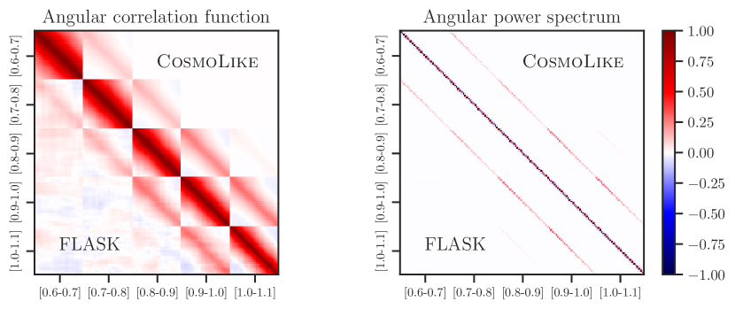
Figure 2: Comparison of correlation matrices obtained from CosmoLike (upper right triangles) and from 2000 FLASK realizations (lower left triangles). The left panel shows the ACF correlation matrix, while the right panel corresponds to the APS one.

We rely on analytic estimates for our fiducial covariance computation, which we validate against covariances estimated from mocks. Following Crocce et al. (2011b), the real space covariance of the angular correlation function $w(\theta)$ at angles $\theta$ and $\theta^{\prime}$ is related to the covariance of the angular power spectrum by

$$\mathrm{Cov}(w(\theta),\,w(\theta^{\prime}))=$$ (17)

$$\sum_{\ell,\,\ell^{\prime}}\dfrac{(2\ell+1)(2\ell^{\prime}+1)}{(4\pi)^{2}}\overline{P_{\ell}}(\theta)\overline{P_{\ell^{\prime}}}(\theta^{\prime})\mathrm{Cov}(C_{\ell},C_{\ell^{\prime}}),$$

where $\overline{P_{\ell}}(\theta)$ are the Legendre polynomials averaged over each angular bin $[\theta_{\min},\,\theta_{\max}]$ and are defined by

$$\overline{P_{\ell}}=\dfrac{\int_{x_{\min}}^{x_{\max}}\mathrm{d}x\,P_{\ell}(x)}{x_{\max}-x_{\min}}=\dfrac{\left[P_{\ell+1}(x)-P_{\ell-1}(x)\right]_{x_{\min}}^{x_{\max}}}{(2\ell+1)(x_{\max}-x_{\min})},$$ (18)

with $x=\cos\theta$ and $x_{\{\min,\,\max\}}=\cos\theta_{\{\min,\max\}}$. In principle, the indices in Equation 17 run for all $\ell$s individually from 0 to $\infty$, although we stop at a large $\ell_{\rm max}$, once convergence is reached.

The covariance matrix $\mathrm{Cov}(C_{\ell},C_{\ell^{\prime}})$ can be split into a Gaussian term (that does not include higher-order moments of the density field), and a non-Gaussian term that involves the 4-point function of the density field (the trispectrum) Takada and Jain (2009) and a super-sample covariance contribution Takada and Hu (2013). We have tested that including these does not impact our results, therefore our fiducial covariance only includes the Gaussian terms. In that case, the covariance of the angular power spectrum in a given tomographic bin is given by Crocce et al. (2011b); Krause and Eifler (2017)

$$\mathrm{Cov}(C_{\ell},C_{\ell^{\prime}})=\dfrac{2\delta_{\ell\ell^{\prime}}}{f_{\rm sky}(2\ell+1)}\left(C_{\ell^{\prime}}+\frac{1}{n_{g}}\right)^{2},$$ (19)

where $\delta$ is the Kronecker delta function, $n_{g}$ is the number density of galaxies per steradian, and $f_{\rm sky}$ is the observed sky fraction, which is used to account for partial-sky surveys.

We use the CosmoLike code to compute the analytical covariance matrices Krause and Eifler (2017); Fang et al. (2020a, b). We include redshift space distortions through the $C_{\ell}$’s of Eq. 19 and, following Troxel et al. (2018), we correct the shot-noise contribution to the covariance (the term $\propto 1/n_{g}$) by taking into account the effect of the survey geometry to the number of galaxies in each angular bin $\Delta\theta$.

For the harmonic space analysis, we begin with the CosmoLike predictions for the angular power spectra and compute analytical Gaussian covariance matrices accounting for broadband binning and partial sky coverage in the PCL estimator context, following Efstathiou (2004); García-García et al. (2019). We compute the coupling terms using the NaMASTER implementation García-García et al. (2019); Alonso et al. (2019).

We have validated both our real space and harmonic space analytic covariance matrices with estimations from simulations, which are described in Section III. The predicted $w(\theta)$ and $C_{\ell}$ from CosmoLike are in very good agreement with the measurements from the mocks, and we also obtain consistent results when using a covariance estimated from either COLA or FLASK mocks (see Tables 2 and 3). In Figure 2 we show that there is good agreement between the correlation matrices obtained from CosmoLike and FLASK mocks. The covariances estimated from COLA are not shown in the Figure 2 and have larger cross-covariance elements due to a replication problem with the mocks, as explained in Ferrero et al. (2021). We refer the reader to Ferrero et al. (2021) for a comparison between CosmoLike and COLA covariances.

IV.4 Parameter Inference

The likelihood function of the parameters $\bm{p}$ given the data $\bm{d}$, $\mathcal{L}$, measures the goodness of the model fit to the data. Under the Gaussian likelihood approximation, the likelihood is related to the $\chi^{2}$ as

$$\mathcal{L}(\bm{p}|\bm{d})\propto e^{-\frac{\chi^{2}}{2}},$$ (20)

where $\chi^{2}$ is given by

$$\chi^{2}(\bm{p}|\bm{d})=\sum_{ij}\big{[}\bm{d}-\bm{M}(\bm{p})\big{]}_{i}C^{-1}_{\,ij}\big{[}\bm{d}-\bm{M}(\bm{p})\big{]}_{j},$$ (21)

with $C$ being the covariance matrix of $\bm{d}$.

The best fit model $\bm{M}$ can be estimated by looking for the parameters $\bm{p}$ at which the likelihood attains its maximum, i.e. the maximum likelihood estimator. The procedure of $\chi^{2}$ minimization given the nuisance parameters in Eq. 14 are similar to those described in Chan et al. (2018). We first analytically fit the linear parameters for the broadband terms $a_{i}$ in Eq. 15 or 16. The residual $\chi^{2}$ is further numerically minimized with respect to the amplitude parameter $B$ subject to the condition that $B>0$. We are left with $\chi^{2}$ of single parameter $\alpha$, whose minimum gives the best fit $\alpha$.

In this work, ${\bf d}$ represents the data from the auto-correlation of each redshift bin. We studied in Chan et al. (2018) the possibility of including cross-correlations between bins, finding that the gain was very small and at the cost of increasing significantly the size of the data vector and its covariance.

In the case of Gaussian likelihood, the 1-$\sigma$ error bar for one single parameter ($\alpha$ in our case) is given by the condition that $\Delta\chi^{2}\equiv\chi^{2}(p)-\chi^{2}(p_{0})=1$, where $\chi^{2}(p_{0})$ is evaluated at the best fit $p_{0}$. We will quote the 1-$\sigma$ error bar derived from this criterion. We will see in Sec. V that this error bar agrees reasonably well with the distribution of the best fit $\alpha$ from the mock results. However, there remains small but non-negligible differences, which indicate deviation from the Gaussian likelihood; thus, we will provide the likelihood for $\alpha$ when the cosmological constraints are desired. We use exclusively the frequentist $\chi^{2}$ fitting to extract the best fit parameters, as we checked that it gives consistent results to the Bayesian method in Chan et al. (2018) (see also Cuceu et al. (2020)).

The template is computed in the fiducial cosmology, and the cosmological information is encoded in the angular BAO scale. The BAO shift parameter $\alpha$ bridges the angular BAO scales in the actual cosmology and the fiducial one as

$$\alpha=\frac{D_{M}(z)}{r_{\rm d}}\frac{r^{\rm fid}_{\rm d}}{D^{\rm fid}_{M}(z)},$$ (22)

where the above expression is evaluated at the effective redshift of the sample, described below. In Eq. (22) $r_{\rm d}$ is the sound horizon at the drag epoch, $D_{M}$ is the (comoving) angular diameter distance and ${\rm fid}$ denotes the fiducial cosmology used for the analysis.

We define the effective redshift as the weighted mean redshift of the sample

$$z_{\rm eff}=\frac{\sum_{i}w_{i,{\rm sys}}\cdot w_{{\rm FKP}}(z_{i})\cdot z_{i}}{\sum_{i}w_{i,{\rm sys}}\cdot w_{{\rm FKP}}(z_{i})}=0.835\,,$$ (23)

with $w_{i,{\rm sys}}$ the systematic weight of the galaxies and the $w_{{\rm FKP}}$ the statistical inverse-variance weight, see Eq.  16 of Ross et al. (2017). This definition was also used for the DES Y1 BAO analysis. We note that alternative definitions can lead to changes in $z_{\rm eff}$ of up to $\Delta z_{\rm eff}\sim 0.035$. However, since in BAO measurements the $D_{M}(z_{\rm eff})$ is divided by the fiducial value $D_{M}^{\rm fid}(z_{\rm eff})$, see Eq. (22), they are not very sensitive to changes in $z_{\rm eff}$, as long as we assume a smooth evolution of $D_{M}(z)$ both at the fiducial and underlying cosmology. For example, for a change from MICE to Planck cosmology, an error of $\Delta z_{\rm eff}=0.035$ translates to an error of $\Delta\alpha=0.001$, well below the statistical uncertainties reported here.

In summary, for MICE cosmology $r_{\rm d}=153.4\,\mathrm{Mpc}$ while $D_{M}(0.835)=2959.7\,\mathrm{Mpc}$, leading to $D_{M}/r_{\rm d}=19.29$. For Planck cosmology $r_{\rm d}=147.6\,\mathrm{Mpc}$ while $D_{M}(0.835)=2967.01\,\mathrm{Mpc}$, leading to $D_{M}/r_{\rm d}=20.1$.

IV.5 Combining Statistics

For consistency and robustness we derive angular distance measurements from real and harmonic space statistics. Even if the angular power spectrum (APS) and the angular correlation function (ACF) contain similar information, the two analyses have been developed using different techniques. In addition, the systematic uncertainties in each one could be different. The compatibility of the two values is a robustness test of the measurement and, given their different sensitivities, both values can be still combined to gain some precision in the final BAO scale measurement. However, the two measurements are highly correlated, and the combination must be done carefully, taking into account the high level of correlation.

As we will see in Sec. V the standard deviations for both measurements are very similar, independently of the covariance matrix we used in the fits (we used COLA mocks, CosmoLike mocks and FLASK mocks). This means that the two analyses have similar sensitivity and similar statistical power, and that some margin for gains exists. To take into account these properties in our combination, we consider two different methods for combining the measurements.

$\bullet$ Method 1 : In the first method we average the $\chi^{2}$ distributions for each measurement to obtain the combined result. This is equivalent to defining the combined likelihood as the geometric mean of the likelihoods from each space, $\mathcal{L(\alpha)_{\rm comb}}=(\mathcal{L(\alpha)_{\rm APS}}\mathcal{L(\alpha)_{\rm ACF}})^{1/2}$. This approach is conservative in the sense that it ignores the correlation of the measurements and will tend to over-estimate the combined error. Nonetheless we will consider this our fiducial method.

$\bullet$ Method 2 : This assumes that the individual likelihoods are Gaussian and uses the combination of two correlated Gaussian variables to obtain the final result. Let us call $\rho$ the Pearson correlation coefficient for the two sets of measurement. Then, the correlation matrix between the ACF and the APS $\alpha$’s is given by

$$\text{corr}(\alpha^{\text{ACF}},\alpha^{\text{APS}})=\begin{pmatrix}1&\rho\\ \rho&1\end{pmatrix}.$$ (24)

Now, we define

$$\sigma_{1}=\sigma_{\alpha}^{\text{ACF}}\quad\sigma_{2}=\sigma_{\alpha}^{\text{APS}}.$$ (25)

Assuming correlated Gaussian distributions, the combined $\alpha$ and its error are given by

$$\alpha^{\text{combined}} =w\alpha^{\text{ACF}}+(1-w)\alpha^{\text{APS}},$$ (26)

$$\sigma_{\alpha}^{\text{combined}} =\left[\frac{(1-\rho^{2})\sigma_{1}^{2}\sigma_{2}^{2}}{\sigma_{1}^{2}+\sigma_{2}^{2}-2\rho\sigma_{1}\sigma_{2}}\right]^{1/2},$$ (27)

where $w$ is defined as

$$w=\frac{\sigma_{2}^{2}-\rho\sigma_{1}\sigma_{2}}{\sigma_{1}^{2}+\sigma_{2}^{2}-2\rho\sigma_{1}\sigma_{2}}.$$ (28)

Note that in those cases where the error difference is too large given the correlation coefficient the weights may be negative. In order to avoid negative contribution from one of the measurements, we will discard those cases.

As we will see below, the correlation coefficient is very high for the case of study here: $\rho=0.893$.

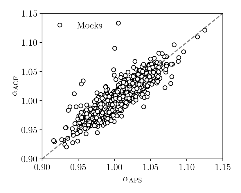
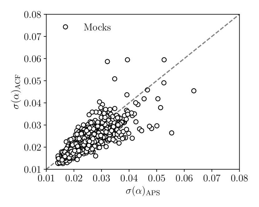
Figure 3: Comparison between the recovered BAO fit (top) and its uncertainty (bottom) from the ACF and the APS on the 1952 ICE-COLA mock realizations (white circles). The $1-\sigma$ errors from APS are $\sim 10\%$ larger than those from ACF, but agree better with the standard deviation from the $\alpha$ distributions on the top panel.

V Tests on Mocks

We have carried out a series of tests to verify our BAO fitting pipeline using the 1952 COLA mocks. The tests are similar to those performed in Chan et al. (2018); Camacho et al. (2019); Dark Energy Survey Collaboration et al. (2019). Table 2 and 3 show the major mock tests for $w$ and $C_{\ell}$ respectively.

A number of metrics are used to quantify the accuracy of the BAO fitting procedures. Recall that in this paper we define the best-fit $\alpha$ through a maximum likelihood estimator and the 1-$\sigma$ error, $\sigma_{\alpha}$, through the condition $\Delta\chi^{2}\equiv 1$, as discussed in Sec. IV.4. Figure 3 shows the distribution of $\alpha$ (upper panel) and $\sigma_{\alpha}$ (lower panel) obtained in $w(\theta)$ vs. $C_{\ell}$ space.

In Table 2 and 3 the distribution of the best fit $\alpha$ derived from the mocks is quantified by its mean, $\langle\alpha\rangle$, and two measures of the spread of the distribution: the standard deviation $\sigma_{\rm std}$ and $\sigma_{68}$. The latter is defined as the symmetric error bar between the $16^{\rm th}$ and $84^{\rm th}$ percentile of the distribution and it is less sensitive to the tails of the distribution compared to $\sigma_{\rm std}$. The mean of the error bar derived from the likelihood $\langle\sigma_{\alpha}\rangle$ is also shown. For the error bar to be meaningful, it should agree with the measures of the spread of the distribution. Another way to quantify the accuracy of the error bar is to check the fraction of mocks enclosing $\langle\alpha\rangle$, i.e. with $\langle\alpha\rangle-\sigma_{\alpha}\leq\alpha\leq\langle\alpha\rangle+\sigma_{\alpha}$, which is 68% from the Gaussian expectation. The pull statistics $d_{\rm norm}=(\alpha-\langle\alpha\rangle)/\sigma_{\alpha}$ enables us to study the correlation between the deviation of the individual best fit from the ensemble one and the error bar derived from the fit. We have shown the mean and the standard deviation of the distribution of $d_{\rm norm}$, $\langle d_{\rm norm}\rangle$ and $\sigma_{d_{\rm norm}}$. The goodness of the fit is indicated by the mean chi-squared per degree of freedom, $\langle\chi^{2}\rangle/\mathrm{d.o.f.}$ To give a representative fit result, we show the fit to mean of mocks using the covariance for a single mock.

The fiducial cosmology for the mock test (template and covariance) is the MICE cosmology and the fiducial covariance estimation is from CosmoLike . For the $w$ fit to the mocks, the fiducial template is computed with $\Delta\theta=0.2^{\circ}$, and the fitting is performed in the angular range $\left[0.5^{\circ},5^{\circ}\right]$. The default number of broadband terms is $\sum_{i}A_{i}/\theta^{i}$ with $i$ going over 0, 1, and 2. For the APS, the default setup is defined by linear piece-wise bandpowers of width $\Delta\ell=20$ with $\ell_{\rm min}=10$ and $\ell_{\rm max}$ derived from a sharp cut of $k_{\rm max}=0.25\,h\,{\rm Mpc}^{-1}$ translated to each tomographic bin using the Limber relation, yielding $\ell_{\rm max}=(410,470,510,550,610)$. For the broadband model we used $A(\ell)=\sum_{i}A_{i}\ell^{i}$ with four terms for $i$ running from -1 to 2. The mock results for this fiducial configuration are shown in bold fonts in Tables 2 and 3, where we also show the results from varying this configuration in terms of the number of broad-band terms, min/max scales, angular binning, and covariance estimation method.

The best fit $\alpha$ from the mean of the mocks is consistent with 1 with a small positive bias which can be attributed to nonlinear evolution of the BAO scale (Crocce and Scoccimarro, 2008; Padmanabhan and White, 2009). This bias ($\sim 0.4\%$) is well below our expected statistical uncertainty ($\sim 2.2\%$) and therefore we consider it negligible and the template construction method described in Sec. IV.2 as unbiased.

In turn, we find that $\langle\sigma_{\alpha}\rangle$ is slightly smaller than $\sigma_{\rm std}$. The differences are smaller for $C_{\ell}$ than for $w$. On the other hand, $\langle\sigma_{\alpha}\rangle$ is closer to $\sigma_{68}$. For $C_{\ell}$, $\langle\sigma_{\alpha}\rangle$ agrees with $\sigma_{68}$ well, while for $w$, $\langle\sigma_{\alpha}\rangle$ is still slightly smaller than $\sigma_{68}$. The discrepancy suggests deviations of the likelihoods from perfect Gaussianity, in particular the ACF. But these deviations are small, with the true errors being underestimated by $\sigma_{\alpha}$ by $\lesssim 10\%$ for ACF (and less so for APS). For both $w$ and $C_{\ell}$, these results are consistent with the fraction of mocks enclosing $\langle\alpha\rangle$ in each case, that for APS yields almost perfectly the expected $68\%$ and for ACF falls short by $\sim 10\%$. The distribution of $d_{\rm norm}$ is close to Gaussian distribution with zero mean and unit variance. The fact that $\sigma_{d_{\rm norm}}$ is slightly larger than 1 follows from the same trend as $\langle\sigma_{\alpha}\rangle$. Overall our model offers a good fit to the mock data and the error estimations are robust and consistent. The ACF likelihood deviates slightly more from perfect Gaussianity than the APS but as we will see next these small discrepancies are removed once ACF and APS are combined.

Table 2: BAO fits for the ACF using the CosmoLike covariance on the COLA mocks with different configurations and variations of the analysis. The form of the broadband terms is $\sum_{i}A_{i}/\theta^{i}$. We also show the results from the angular binning $\Delta\theta$ and the minimum angular scale considered $\theta_{\rm min}$. We have also tested the results obtained with the COLA mock-based covariance or the one from FLASK mocks. In the next row, Planck cosmology is assumed for both the BAO template and the CosmoLike covariance. Finally, in order to check the number of broadband terms required to get an unbiased estimate for an alternative cosmology template, we have shown the results obtained with the Planck cosmology template for different number of broadband terms. The bold entries indicate our baseline choice, in addition to $\theta_{\rm min}=0.5\deg$ and $\theta_{\rm max}=5\deg$.

case	$\langle\alpha\rangle$	$\sigma_{\rm std}$	$\sigma_{68}$	$\langle\sigma_{\alpha}\rangle$	${\rm fraction\,encl.}\langle\alpha\rangle$	$\langle d_{\rm norm}\rangle$	$\sigma_{d_{\rm norm}}$	$\langle\chi^{2}\rangle/{\rm d.o.f.}$	${\rm mean\,of\,mocks}$
$i=0$	1.002	0.022	0.021	0.021	65%	0.010	1.057	101.5/99 (1.03)	1.002 $\pm$ 0.020
$i=0,1$	1.003	0.024	0.023	0.022	63%	-0.025	1.090	97.6/94 (1.04)	1.003 $\pm$ 0.021
${\bf i=0,1,2}$	1.004	0.024	0.023	0.021	62%	-0.024	1.116	93.1/89 (1.05)	1.004 $\pm$ 0.021
$i=-1,0,1,2$	1.004	0.024	0.023	0.021	63%	-0.026	1.124	88.3/84 (1.05)	1.004 $\pm$ 0.021
$\Delta\theta=0.10\deg$	1.004	0.024	0.023	0.021	64%	-0.019	1.107	198.2/204 (0.97)	1.004 $\pm$ 0.021
$\Delta\theta=0.15\deg$	1.004	0.024	0.023	0.021	63%	-0.019	1.107	129.0/129 (1.01)	1.004 $\pm$ 0.021
${\bf\Delta\theta=0.20\deg}$	1.004	0.024	0.023	0.021	62%	-0.024	1.116	93.1/89 (1.05)	1.004 $\pm$ 0.021
$\theta_{\rm min}=1\deg$	1.004	0.024	0.023	0.021	62%	-0.028	1.120	82.8/79 (1.05)	1.004 $\pm$ 0.021
${\rm COLA\,cov}$	1.004	0.025	0.024	0.023	66%	-0.024	1.055	86.2/89 (0.97)	1.003$\pm$ 0.023
${\rm FLASK\,cov}$	1.004	0.026	0.025	0.022	64%	-0.023	1.098	90.4/89 (1.02)	1.003$\pm$ 0.022
${\rm{\tt Planck}\,cosmology}$	0.966	0.023	0.023	0.026	73%	-0.017	0.880	72.7/89 (0.82)	0.965$\pm$ 0.026
${\rm{\tt Planck}\,temp.}\,i=0$	0.949	0.022	0.022	0.021	64%	0.048	1.05	109.9/99 (1.11)	0.949$\pm$ 0.022
${\rm{\tt Planck}\,temp.}\,i=0,\,1$	0.965	0.023	0.023	0.024	69%	-0.019	0.98	101.5/94 (1.08)	0.965$\pm$ 0.023
${\rm{\tt Planck}\,temp.}\,i=0,\,1,\,2$	0.966	0.023	0.023	0.022	65%	-0.021	1.06	94.3/89 (1.06)	0.965$\pm$ 0.022
${\rm{\tt Planck}\,temp.}\,i=-1,\,0,\,1,\,2$	0.966	0.024	0.022	0.022	65%	-0.027	1.07	89.0/84 (1.06)	0.966$\pm$ 0.022

Table 3: BAO fits for the APS using the CosmoLike covariance on the COLA mocks with different configurations and variations of the analysis. The form of the broadband terms is $A(\ell)=\sum_{i}A_{i}\ell^{i}$. We also show the results from the broadband binning $\Delta\ell$ and the maximum multipole considered $\ell_{\mathrm{max}}$. Next, we consider the change of the method for computing the covariance. In the next row, Planck cosmology is assumed for both the BAO template and the CosmoLike covariance. Finally, to check the number of broadband terms required to get an unbiased estimate for an alternative cosmology template, we have shown the results obtained with the Planck cosmology template for different number of broadband terms. The bold entries indicate the baseline choice, in addition to $\ell_{\rm min}=10$ and $\ell_{\rm max}=(410,470,510,550,610)$ for each bin (see text for details).

case	$\langle\alpha\rangle$	$\sigma_{\rm std}$	$\sigma_{68}$	$\langle\sigma_{\alpha}\rangle$	${\rm fraction\,encl.}\langle\alpha\rangle$	$\langle d_{\rm norm}\rangle$	$\sigma_{d_{\rm norm}}$	$\langle\chi^{2}\rangle/{\rm d.o.f.}$	${\rm mean\,of\,mocks}$
$i=0$	1.006	0.020	0.019	0.019	68%	-0.005	1.043	118.5/114 (1.04)	1.006 $\pm$ 0.019
$i=0,1$	1.002	0.023	0.021	0.022	69%	0.020	1.045	113.2/109 (1.04)	1.002 $\pm$ 0.021
$i=0,1,2$	1.003	0.023	0.022	0.022	68%	0.026	1.041	107.9/104 (1.04)	1.003 $\pm$ 0.022
${\bf i=-1,0,1,2}$	1.004	0.025	0.023	0.023	69%	-0.008	1.050	100.9/99 (1.02)	1.004 $\pm$ 0.023
$\Delta\ell=10$	1.004	0.024	0.023	0.022	67%	-0.008	1.059	229.9/226 (1.02)	1.004 $\pm$ 0.022
${\bf\Delta\ell=20}$	1.004	0.025	0.023	0.023	69%	-0.008	1.050	100.9/99 (1.02)	1.004 $\pm$ 0.023
$\Delta\ell=30$	1.004	0.027	0.024	0.024	68%	-0.011	1.063	58.5/57 (1.03)	1.004 $\pm$ 0.024
$\ell_{\rm max}=550$	1.004	0.025	0.023	0.023	67.5%	-0.013	1.061	112.8/109(1.03)	1.004 $\pm$ 0.023
${\rm COLA\,cov}$	1.004	0.025	0.023	0.024	71%	-0.010	0.974	92.6/99 (0.94)	1.004 $\pm$ 0.023
${\rm FLASK\,cov}$	1.004	0.026	0.024	0.023	67%	-0.006	1.079	102.4/99 (1.03)	1.004 $\pm$ 0.023
${\rm{\tt Planck}\,cosmology}$	0.965	0.024	0.022	0.028	78%	-0.002	0.835	76.5/99 (0.77)	0.965 $\pm$ 0.027
${\rm{\tt Planck}\,temp.}\,i=0$	0.917	0.024	0.023	0.022	67%	0.101	1.076	133.2/114 (1.17)	0.918$\pm$ 0.022
${\rm{\tt Planck}\,temp.}\,i=0,\,1$	0.947	0.025	0.023	0.023	66%	0.066	1.068	121.9/109 (1.12)	0.948$\pm$ 0.022
${\rm{\tt Planck}\,temp.}\,i=0,\,1,\,2$	0.957	0.022	0.021	0.021	68%	0.044	1.046	111.3/104 (1.07)	0.958$\pm$ 0.020
${\rm{\tt Planck}\,temp.}\,i=-1,\,0,\,1,\,2$	0.966	0.023	0.022	0.023	70%	-0.005	0.993	102.0/99 (1.03)	0.966$\pm$ 0.022

For the MICE cosmology template, the fit results are only weakly dependent on the number of braodband terms with the effects on $C_{\ell}$ being more apparent. We will see below that this is more important when we consider a different cosmology for the template and this will drive the number of broad-band terms used by defaults. For $w$, a number of angular bin widths $\Delta\theta$ are considered: $0.10^{\circ}$, $0.15^{\circ}$, and $0.20^{\circ}$. The results are insensitive to the angular bin width, and we find that the $\chi^{2}/{\rm d.o.f.}$ increases mildly with the increase of the bin width. To reduce the size of the covariance matrix, we adopt $0.20^{\circ}$ as the fiducial setup. Similarly, for $C_{\ell}$, the results for $\Delta\ell=10$, 20, and 30 are shown. For $\Delta\ell=30$, the difference between $\sigma_{\rm std}$ and $\langle\sigma_{\alpha}\rangle$ is marked, while for smaller $\Delta\ell$, the difference reduces. Again as a compromise for the size of the covariance matrix, we adopt $\Delta\ell=20$ as the fiducial setup. Using a minimum angular scale $\theta_{\rm min}=1^{\circ}$ for $w$, the results are basically unchanged and this suggests the results are not sensitive to the small scales. We conclude that changing the fiducial analysis configuration does not introduce quantitative differences in the results.

Tables 2 and 3 also display the results obtained using COLA and FLASK covariance for reference. Overall the COLA covariance gives very consistent results, especially for $w$, e.g. $\langle\sigma_{\alpha}\rangle$ and $\sigma_{\rm std}$ (or $\sigma_{\rm 68}$) are closer to each other. This is reassuring since this estimation traces the actual mock statistics. However, the overlapping issue mentioned previously casts doubt on its validity for the real data. Furthermore, it is only available in the MICE cosmology. For the FLASK covariance, we find slightly larger difference between $\langle\sigma_{\alpha}\rangle$ and $\sigma_{\rm std}$ (or $\sigma_{\rm 68}$).

The next entries of Tables 2 and 3 show the results obtained assuming a Planck cosmology (Planck template plus the Planck covariance). The theoretically expected value for fitting MICE mocks with a Planck template (by comparing the sound horizon and the angular diameter distance) is 0.959, if we consider the 0.004 shift found in the mocks due to non-linearities, we are left with an expectation of 0.963. Hence, finding an additional small bias of 0.003 or 0.002 when comparing to the $\langle\alpha\rangle$ in the Planck cosmology entry of Tables 2 & 3, respectively. Nevertheless, this bias is negligible when compared to the error bars. The fact that the magnitude of the covariance elements are generally larger in Planck cosmology can explain that $\sigma_{\alpha}$ and fraction enclosing $\langle\alpha\rangle$ are higher while $\chi^{2}/\mathrm{d.o.f.}$ and $\sigma_{d_{\rm norm}}$ are lower. The last set of entries in Tables 2 and 3 consider fitting the COLA mocks (based on MICE cosmology) with the Planck template (but still the MICE covariance) for different number of broad-band parameters. In this case, it is very clear that the number of broad-band parameters is very important to recover unbiased results. For APS, we find that we need at least 4 ($i=-1,0,1,2$) broad-band parameters so that results converge (not shown here, but results are consistent when using more parameters). For the ACF, we find that 2 or 3 parameters are sufficient to get stable results. For this case, we consider 3 parameters ($i=0,1,2$) in order to allow for more flexibility.

Table 4: Results of BAO fits in mock catalogs. The results of ACF and APS are combined using two methods, described in Sec. IV.5.

case	$\langle\alpha\rangle$	$\sigma_{\rm std}$	$\sigma_{68}$	$\langle\sigma_{\alpha}\rangle$	${\rm fraction\,encl.}\langle\alpha\rangle$	$\langle d_{\rm norm}\rangle$	$\sigma_{d_{\rm norm}}$	${\rm mean\,of\,mocks}$
$w(\theta)$	1.004	0.024	0.023	0.021	62%	-0.024	1.112	1.004 $\pm$ 0.021
$C_{\ell}$	1.004	0.025	0.023	0.023	69%	-0.008	1.050	1.004 $\pm$ 0.023
$w(\theta)+C_{\ell}$ [method 1: FID]	1.004	0.024	0.022	0.022	67%	-0.017	1.054	1.004 $\pm$ 0.022
$w(\theta)+C_{\ell}$ [method 2]	1.004	0.023	0.022	0.021	65%	-0.017	1.102	1.004 $\pm$ 0.021

As discussed before we expect our fiducial result to come from the combination of ACF and APS. For combining these two highly correlated statistics we put forward two slightly different methods, presented in Sec. IV.5. The combined statistic from both combination methods are shown in Table 4. Using method 1, that considers the geometric mean of the individual likelihoods, we find a mean combined value of $\langle\alpha\rangle=1.004$ with a mean combined error $\langle\sigma_{\alpha}\rangle=0.022$. This mean error coincides perfectly with the $68\%$ distribution of combined best-fit $\alpha$ values and is smaller than the standard deviation $\sigma_{\rm std}$. The pull statistics using $d_{\rm norm}$ agree to within $5\%$ with that corresponding to a unitary Gaussian. For method 2 we first measure the Pearson correlation coefficient from all the mock measurements, yielding $\rho=0.893$. Using this value we estimate the weight per mock and the combined $\alpha$ statistics as shown in Table 4. Alternatively, we also tried using the weights derived from the mean error of the mocks, yielding very similar statistics (not explicitly shown here). In method 2, we eliminated by default the mocks that have negative values for either of the weights, this is 35% of the mocks. Given how often this happens, we also tried including those mocks in the ensemble, only resulting in very minor changes to the statistics in Table 4. We do not enter into details these alternative methods and we do not include their values in Table 4, as neither of them is chosen as the fiducial option. We leave for Y6 a more detailed exploration of the methods for the combined constraints.

The results using method 2 are very consistent with those from method 1, with a slightly larger deviation from Gaussian statistics. In all, both methods produce very similar final results but we will consider method 1 as our fiducial. The improvement on the measurement error coming from the combination of ACF and APS is of $\sim 5\%$ on the mocks.

VI Pre-unblinding tests

In order to avoid confirmation bias, the analysis was performed blind. While blinded, we do not compute $\alpha$ on the final data vector, and do not plot the ACF or APS. Before un-blinding, we require passing a set of tests designed to identify any issues in the analysis without being influenced by confirmation bias. The pre-unblinding tests are the following,

1. Is the BAO detected? We consider to have a detection if the $1\sigma$ region of posterior of the $\alpha$ parameter (using all 5 tomographic bins) lies inside the prior range $[0.8,1.2]$, i.e, the $\alpha\pm 1\sigma_{\alpha}$ is within our (flat) prior limit. We find this test to pass for the DES Y3 BAO sample data. This interval is 10 times larger than the expected error in $\alpha$, and we can know if the measurement satisfies this constraint without violating the blinding protocol.

2. Is the measurement robust? We test the impact in $\alpha$ from variations in the analysis. In order to remain blinded we only refer to variations in $\alpha$ with respect to a fiducial analysis, defining a variable $\Delta=\alpha_{\rm variation}-\alpha_{\rm fid}$ in each case. We repeat this process on mocks and consider the data to have passed an individual test if we find $\Delta\alpha^{\rm data}$ to be within the $90\%$ confidence interval of $\Delta\alpha^{\rm mock}$. If one or more tests do not pass, we consider the ensemble statistic of all tests to determine the likelihood of such a failure (similarly if two or more tests do not pass, etc). If the ensemble probability of such a failure is $10\%$ or more we consider the failure statistically justified and move on. If it is less than $10\%$ but larger than $1\%$ we delay the unblinding stage to re-evaluate all the analysis process. If we find nothing in the process that needs to be changed we move on. If the ensemble probability of such failure is below $1\%$, and remains so after the revision, the unblinding is not allowed. The individual tests are the following,

   • Impact of removing one tomographic bin. We test the change in best-fit $\alpha$ when removing one tomographic bin at a time and compare to the equivalent distribution in the COLA mocks. The quantity being measured on both the mocks and data is $\Delta=\alpha_{4-\rm bins}-\alpha_{5-\rm bins}$. For the mocks this test is done using a MICE cosmology template (corresponding to the true cosmology of the mocks). For the data we perform the test with Planck or MICE cosmologies. The results are shown in the top five rows of Tables 5 and 6. We also test the impact of removing tomographic bins on the estimated uncertainty $\sigma_{\alpha}$, which is displayed in the bottom part of each table. The result on the data agrees well with the distributions on the mocks. While this is not a pre-unblinding requirement in itself we regard it as informative.

   • Impact of template cosmology. We test that our results vary with the assumed cosmology template as expected from the change in cosmology itself. Hence we perform the BAO fits assuming either a MICE or Planck template (using the same covariance). From these cosmologies we theoretically expect to find a difference in $\alpha$ of 0.041. However, in Table 2 & Table 3 we found that, for the mocks, the mean shift of $\alpha$ is 0.038 & 0.039 for the ACF & APS statistics, respectively. Hence we consider the variable $\Delta=(\alpha_{\rm Planck}-\alpha_{\rm MICE}+0.039)$, which should be centered around zero for the APS and around 0.001 for the ACF. The results are shown in the sixth row of Tables 5 and 6 (under column MICE for the data).

   • Impact of covariance cosmology. We measure the distribution of best fit $\alpha$ when using CosmoLike covariance with MICE cosmology and bias values (our default for these set of tests) or Planck cosmology (with its corresponding refitted galaxy bias). The variable here is $\Delta=\alpha_{\rm Planck\ {\textsc{CosmoLike}}}-\alpha_{\rm MICE\ {\textsc{CosmoLike}}}$. Results are displayed in the seventh row to Tables 5 and 6.

   • Impact of n(z) estimation. We test that our results are robust with respect to the estimation of the underlying redshift distributions. We compare the best fit $\alpha$ when fitting with BAO templates obtained with a redshift distribution from VIPERS direct calibration or using the stacking of DNF Z_MC, see Sec. II.3 and Carnero Rosell et al. (2021). The variable is $\Delta=(\alpha_{\textsc{DNF}-\texttt{\small Z\_MC}}-\alpha_{\rm VIPERS})$. We compare this to the same quantity on the COLA mocks. We perform this test for two different cosmologies, and the results are shown in the eighth row of the table.

   These tests are summarised in Tables 5 and 6. The test removing the 5th redshift bin fails at 90% Confidence Level (CL) for the power spectrum and at 97% CL for the correlation function. We also find that the test of the impact of template cosmology is failed at the 90% level for the correlation function. All other tests pass. For the power spectrum, 43% of mocks had one or more test fail at 90% CL, so we consider that the APS passes very clearly the pre-unblinding tests. For the correlation function 17% of mocks has one or more test fail at 97% CL and 22% of mocks fail 2 tests at 90% CL. Since more than 5% of mocks fail the same number of robustness tests, given the CL intervals, we consider this pre-unblinding test to pass. Additionally, below, we consider the ensemble of robustness tests all together.

3. Is it a likely draw? We measure the covariance of the $\Delta\alpha$ for each of the above tests from the COLA mocks (i.e. an $8\times 8$ covariance given the 8 different tests, estimated from 1952 mocks). We compute the $\chi^{2}$ for each mock $\Delta\alpha$ from this covariance. If $\chi^{2}_{\rm data}>99\%$ of the $\chi^{2}_{\rm mock}$ distribution we consider this test to have failed. If $99\%>\chi^{2}_{\rm data}>95\%$ of the $\chi^{2}_{\rm mock}$, we consider this to warrant further investigation. On the real data we find the angular power spectrum $\Delta\alpha$ to have $\chi^{2}=3.58$, much less than the 95% threshold of 22.4. The angular correlation function $\Delta\alpha$ has $\chi^{2}=12.5$, much less than the 95% threshold of 22.5.

4. Is it the BAO a good fit? We compare the goodness of fit of the $w(\theta)$ fit itself, comparing the $\chi^{2}$ measured on the data to the same value as the mocks. We again consider a p-value of $<1\%$ to be a failed test and $<5\%$ to warrant further investigation. These $\chi^{2}$ values are shown in Table LABEL:tab:baodata, all the corresponding p-values pass the $1\%$ threshold.

For the pre-unblinding tests that require measuring $\alpha$ on the real data we apply an unknown random offset to all $\alpha$ measurements to keep the true measurement blind (besides considering only $\Delta\alpha$ statistics). Since we passed all the pre-unblinding conditions, we proceeded to the final stage.

Table 5: Table of pre-unblinding tests for the Angular Power Spectrum from Section VI, showing the impact of removing individual tomographic bins, of changing the assumed cosmology for the BAO template or the covariance, and of considering an independent estimate of the true redshift distributions. We report variations in $\alpha$ with respect to our fiducial analysis, to keep results blind. The first four columns show the range of $\Delta\alpha$ values measured on the COLA mocks that enclose the fraction of mocks shown at the top of each column. By default the mocks are analysed assuming MICE cosmology. The fifth column shows the $\Delta\alpha$ value measured on the data, for two different fiducial cosmologies, MICE and Planck. A test (each row) is said to have failed if the data value falls outside of the bounds measured on the mocks. For the Angular Power Spectrum, only one test ("1234" removing the fifth redshift bin) fails at the 90% threshold. Considering the whole ensemble of tests (all rows), we find 43% of mocks have one or more failed test at the 90% threshold. Hence this failure was not considered an issue for unblinding. The bottom raws show the impact of removing one bin at a time on the error in $\alpha$ (but this does not impose conditions on unblinding).

Threshold	0.9		0.95		0.97		0.99		data
(Fraction of mocks)	min	max	min	max	min	max	min	max	MICE	Planck
	$10^{2}(\alpha-\alpha_{\rm fiducial})$
Bins 2345	-1.58	1.73	-2.22	2.18	-2.65	2.73	-4.33	4.46	0.92	1.17
1345	-1.8	1.88	-2.36	2.43	-2.84	2.84	-4.35	3.68	-0.62	-0.46
1245	-1.87	2.07	-2.55	2.76	-3.04	3.49	-4.26	5.92	-0.34	-0.26
1235	-2.01	1.84	-2.77	2.39	-3.29	3.06	-4.44	4.62	-0.84	-1.02
1234	-2.28	1.75	-3.13	2.35	-3.49	2.78	-5.14	3.77	1.58	1.83
Planck Template	-0.66	0.72	-0.88	0.87	-1.08	1.07	-1.48	1.37	0.10	-
Planck Covariance	-0.41	0.47	-0.53	0.59	-0.59	0.74	-0.85	0.9	-0.16	-
$n(z)_{\textsc{DNF}-{\rm Z_{\rm MC}}}$	-0.73	0.12	-0.87	0.21	-0.96	0.29	-1.13	0.46	-0.13	-0.19
	$(\sigma-\sigma_{\rm All\ Bins})/\sigma_{\rm All\ Bins}$
Bins 2345	-0.05	0.30	-0.09	0.38	-0.12	0.44	-0.18	0.59	0.00	0.05
1345	-0.06	0.31	-0.08	0.38	-0.12	0.44	-0.18	0.62	0.09	0.10
1245	-0.04	0.37	-0.08	0.47	-0.10	0.52	-0.18	0.82	0.10	0.05
1235	-0.06	0.37	-0.1	0.44	-0.13	0.56	-0.19	0.75	0.23	0.08
1234	-0.06	0.36	-0.1	0.44	-0.12	0.50	-0.19	0.69	0.19	0.09

Table 6: As table 5 but for the Angular Correlation Function. We find one test ("1234" removing the fifth redshift bin) fails at the 97% threshold. We find 17% of mocks have one or more failed test at the 97% threshold so this was not considered an issue for unblinding.

Threshold	0.9		0.95		0.97		0.99		data
(Fraction of mocks)	min	max	min	max	min	max	min	max	MICE	Planck
	$10^{2}(\alpha-\alpha_{\rm fiducial})$
Bins 2345	-1.60	1.84	-2.27	2.42	-2.76	2.92	-4.20	3.78	1.12	0.92
1345	-1.80	1.84	-2.22	2.36	-2.76	2.92	-3.84	4.30	-1.24	-1.08
1245	-1.92	1.99	-2.52	2.68	-3.27	3.00	-4.81	4.64	-0.68	-0.26
1235	-1.88	1.84	-2.60	2.34	-3.11	2.87	-4.15	4.02	-1.44	-1.02
1234	-1.95	1.68	-2.56	2.26	-3.12	2.68	-4.15	3.68	3.44	2.84
Planck Template	-0.38	0.54	-0.50	0.66	-0.58	0.74	-0.70	0.90	0.61	-
Planck Covariance	-0.40	0.36	-0.52	0.48	-0.60	0.55	-0.77	0.76	0.08	-
$n(z)_{\textsc{DNF}-{\rm Z_{\rm MC}}}$	-0.80	0.12	-0.92	0.20	-1.00	0.31	-1.21	5.21	0.00	-0.12
	$(\sigma-\sigma_{\rm All\ Bins})/\sigma_{\rm All\ Bins}$
Bins 2345	-0.04	0.30	-0.06	0.36	-0.10	0.42	-0.14	0.62	0.05	0.05
1345	-0.04	0.33	-0.06	0.40	-0.09	0.47	-0.15	0.58	0.04	0.05
1245	-0.04	0.37	-0.07	0.45	-0.09	0.54	-0.16	0.74	0.12	0.11
1235	-0.05	0.35	-0.08	0.43	-0.11	0.53	-0.11	0.53	0.09	0.12
1234	-0.05	0.35	-0.07	0.40	-0.09	0.45	-0.14	0.70	0.07	0.07

VII Results

The different methods previously discussed produce BAO detections in both real and harmonic space. We study the compatibility of these detections and their combination, that yield a precise determination of the angular diameter distance to $z=0.835$.

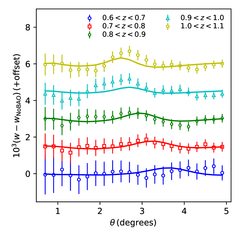
Figure 4: The isolated BAO feature, measured in configuration space using the angular correlation function, $w(\theta)$. The measurements have been re-scaled by a factor of 10³ and vertical offsets of +1.5 have been sequentially added with each tomographic bin. The BAO feature moves to lower angular scales as the redshift increases, reflecting constant co-moving size. The error bars are based on the fiducial Planck covariance, neighboring data points are strongly correlated. The solid lines represent the best fit.

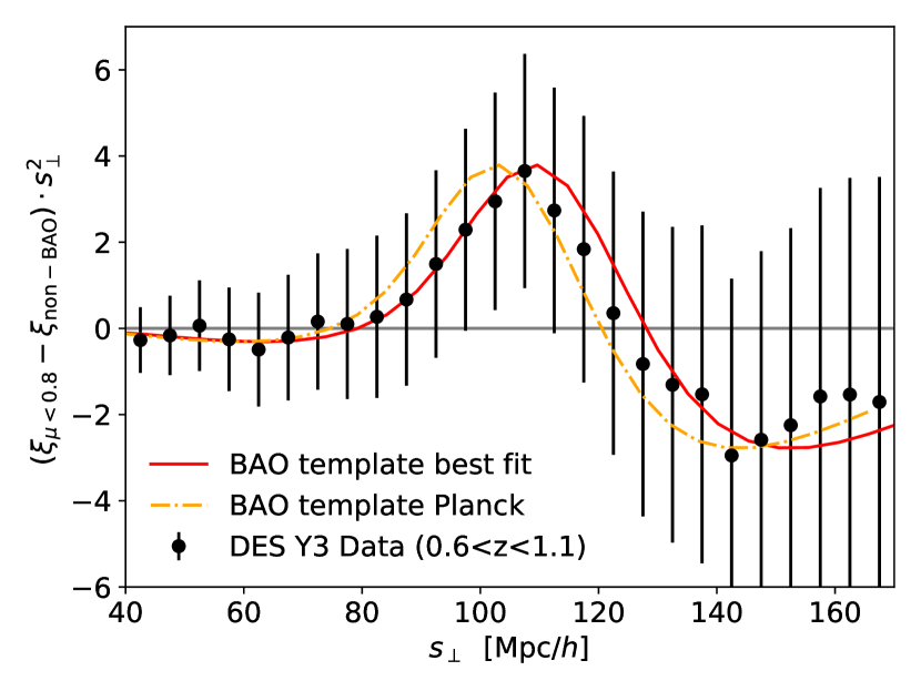
Figure 6: Projected 2-point correlation function as a function of comoving separation perpendicular to the line-of-sight, see Eq. (6). The circles show the measurement on the DES Y3 data with error bars computed from the COLA mocks. The orange dash-dotted line has been shifted by the parameter $\alpha$ corresponding to Planck cosmology and red solid line by the $\alpha$ corresponding to the best fit to the $w(\theta)$+$C_{\ell}$ data. All curves have been subtracted by a non-BAO template.

VII.1 The BAO signal

The measured BAO signal is shown in Figure 4 for configuration space and in 5 for harmonic space. In order to isolate this signal, we have subtracted (divided) the $w$ ($C_{\ell}$) by the no-BAO smooth prediction from the no-wiggle power spectrum, Eq. (9). To provide better visualization of each tomographic bin, we further introduced vertical offsets, displaying the different tomographic bins from the bottom to the top in increasing redshift order. The BAO feature moves towards lower angular scales (lower $\theta$ for $w$ and higher $\ell$ for $C_{\ell}$) as the redshift increases, reflecting its fixed co-moving scale.

The projected clustering results can be found in Figure 6, where we show the measurements on the data following the procedure explained in Sec. IV.1.3, compared to two theoretical curves. First, the MICE theory template was created using MICE cosmology, the biases $b(z_{i})$ used for the COLA galaxy mocks and the theory from Section IV.2 projected to $s_{\perp}$-space using a framework similar to what is described in Ross et al. (2017). Additionally, a non-BAO template is created in a similar fashion for the $w(\theta)$ and $C_{\ell}$ statistics, which is subtracted from all the other curves. We then shift the templates using the $\alpha$ parameter corresponding to the Planck cosmology and to the best fit BAO resulting from the combination of ACF and APS. The templates are rescaled by a factor of $B^{2}=0.9$ in order to match the amplitude of the DES Y3 clustering at large scales. The errors are computed from the standard deviation of 200 COLA mocks, and both data and mock pair-counts assume MICE cosmology. We only use the projected clustering for display purposes since it is the single correlation with highest signal-to-noise, but not to derive distance measurements.

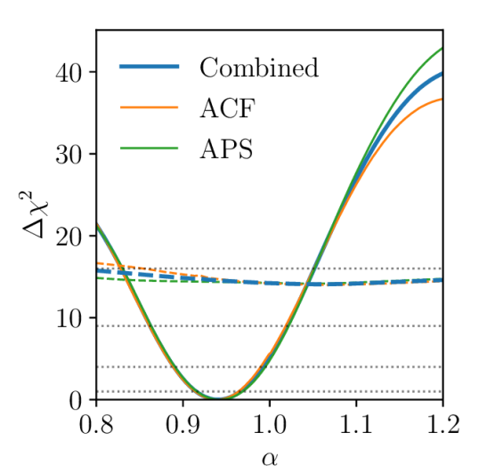
Figure 7: The BAO likelihood for the DES Y3 BAO sample data, for the configuration space (ACF), the harmonic space (APS) and the combined result using the geometric mean of the individual likelihoods. The dashed lines show the recovered likelihood for a model without BAO, indicating a detection of the BAO feature in DES Y3 at greater than than 3$\sigma$ significance level. The dotted black lines denote 1, 2, 3 and 4$\sigma$ levels, based on $x\sigma=\sqrt{\Delta\chi^{2}}$.

VII.2 BAO Distance Measurements

Figure 7 shows the $\Delta\chi^{2}$ for $\alpha$ from the configuration and harmonic space analyses together with their combination. Both $\Delta\chi^{2}$ are remarkably similar, particularly around its minima, diverging mostly for large values of $\alpha$. This consistency between the analyses enables a robust combination. In addition, the result for a model without BAO is also shown, as dashed lines. This model does not describe the data. From these results, a significance of more than $3\sigma$ in the determination of the BAO feature is inferred.

We find that the values of $\alpha$ measured from these likelihoods in each space, i.e. using the 5 redshift bins together, are all compatible. Therefore, we can combine them, obtaining $\alpha=0.937\pm 0.025$ with a $\chi^{2}=95.24$ for 89 degrees of freedom and $\alpha=0.942\pm 0.026$ with a $\chi^{2}=92.26$ for 99 degrees of freedom, for the ACF and APS, respectively. These values are in perfect agreement, with best-fit values, estimated errors and $\chi^{2}$ well within the expectations. Thus, we can also combine the ACF and APS likelihoods, which yields a measurement of $\alpha=0.941\pm 0.026$. We consider this our official final measurement. The combined likelihood given by the geometric mean of the individual likelihoods is shown by a blue solid line in Fig. 7.

The quality of the Y3 data are high enough to allow us to detect the BAO signals from individual redshift bins. These are shown in Fig. 8. For $w$, the BAO fit results using individual redshift bins are: No detection, $0.997\pm 0.051$, $0.978\pm 0.048$, $0.977\pm 0.038$, and $0.895\pm 0.033$, with $\chi^{2}/{\rm dof}$ given by $13.7/17$, $16.6/17$, $23.1/17$ and $10.1/17$. For $C_{\ell}$ we obtain: No detection, $0.992\pm 0.055$, $0.979\pm 0.053$, $0.971\pm 0.038$, and $0.919\pm 0.040$ with $\chi^{2}/{\rm dof}$ given by $11.9/17$, $13.1/19$, $33.6/21$ and $21.93/24$.

Except for the first bin, which does not meet our detection criteria, BAO signals are detected in individual redshift bins, with the significance increasing with redshift. The fifth bin is the primary driver for the low value of $\alpha$ compared to Planck cosmology. But results are remarkably compatible in real and harmonic space, and the goodness-of-fit is good. We note that the decrease of the error bar size with redshift is more pronounced than the results from mocks, in which the mean error fluctuates in between 0.4 and 0.5.

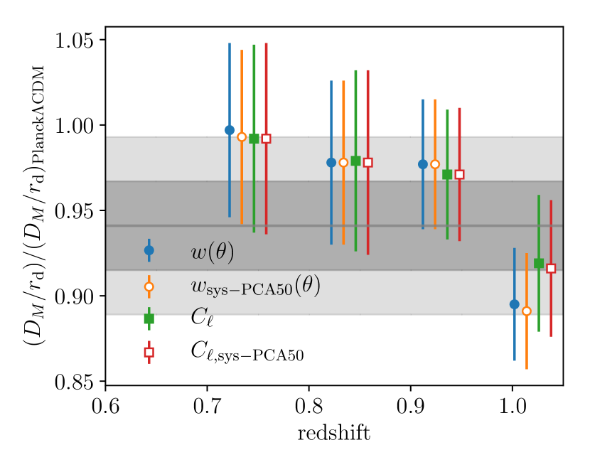
Figure 8: The BAO fit for the individual tomographic bins. The shaded region corresponds to our Y3 choice measurement from the combination of $w(\theta)$ and $C_{\ell}$. We show the individual results for the fiducial analysis and the case of using the PCA50 weights. The largest differences when changing the weights are for the second and fifth bin, being of $\sim 0.1\sigma$ showing the robustness of our measurements to systematic weights.

VII.3 Robustness Tests

All the robustness tests that have been described for mocks have been also applied to the data, in order to check the stability and soundness of the results.

First, we have used a second method to combine ACF and APS results, presented in Sec. IV.5. We assume the Gaussianity for both likelihoods and then combine the results as correlated Gaussian measurements. The correlation between the two $\alpha$ values is obtained from the mocks. The obtained result (Method 2) is perfectly compatible with the fiducial result (Method 1, FID), as can be seen in Table  LABEL:tab:baodata.

Table 7: BAO fits to the Y3 data. Our combined result is shown in the top row, in terms of the ratio of the recovered comoving angular diameter distance at $z_{\rm eff}=0.835$ to the sound horizon scale, for the Planck cosmology. The following rows show various robustness tests conducted, discussed in detail in Sec. VII.3.

Y3 Measurement	$D_{M}/r_{\rm d}$
$z_{\rm eff}=0.835$	$18.92\pm 0.51$
case	$\alpha$	$\chi^{2}$/dof
$w(\theta)+C_{\ell}$ [method 1: FID]	$0.941\pm 0.026$	-
$w(\theta)+C_{\ell}$ [method 2]	$0.939\pm 0.025$	-
Robustness tests:
$w(\theta)$	$0.937\pm 0.025$	$95.2/89$
$w(\theta)$ no ${\rm sys}$	$0.935\pm 0.026$	$94.6/89$
$w(\theta)$ ${\rm sys-PCA50}$	$0.937\pm 0.025$	$94.9/89$
$w(\theta)$ $n(z)$ DNF  PDFs	$0.935\pm 0.025$	$95.6/89$
$w(\theta)$ $\theta_{\rm min}=1^{\circ}$	$0.939\pm 0.025$	$81.7/79$
$w(\theta)$ $\theta_{\rm max}=4^{\circ}$	$0.937\pm 0.025$	$54.7/64$
$w(\theta)$ $\Delta\theta=0.1^{\circ}$	$0.942\pm 0.026$	$220.2/204$
$w(\theta)$ 2345	$0.948\pm 0.026$	$67.8/71$
$w(\theta)$ 1345	$0.929\pm 0.026$	$80.7/71$
$w(\theta)$ 1245	$0.935\pm 0.028$	$78.4/71$
$w(\theta)$ 1235	$0.925\pm 0.028$	$70.0/71$
$w(\theta)$ 1234	$0.967\pm 0.026$	$82.3/71$
$C_{\ell}$	$0.942\pm 0.026$	$92.3/99$
$C_{\ell}$ no ${\rm sys}$	$0.940\pm 0.028$	$89.7/99$
$C_{\ell}$ ${\rm sys-PCA50}$	$0.941\pm 0.026$	$89.7/99$
$C_{\ell}$ $n(z)$ DNF  PDFs	$0.940\pm 0.025$	$92.1/99$
$C_{\ell}$ $\ell_{\rm max}=550$	$0.940\pm 0.026$	$104.6/109$
$C_{\ell}$ $\Delta\ell=10$	$0.939\pm 0.027$	$238.8/226$
$C_{\ell}$ $\Delta\ell=30$	$0.936\pm 0.028$	$40.0/57$
$C_{\ell}$ 2345	$0.954\pm 0.028$	$82.2/84$
$C_{\ell}$ 1345	$0.938\pm 0.029$	$82.0/81$
$C_{\ell}$ 1245	$0.940\pm 0.028$	$79.5/79$
$C_{\ell}$ 1235	$0.932\pm 0.029$	$56.3/77$
$C_{\ell}$ 1234	$0.961\pm 0.029$	$69.1/74$

Then, we apply the full battery of tests as described below.

$\bullet$ Impact of standard weights for systematics. The stability of the measurement with respect to the observational systematics decontamination has been tested by comparing the distribution of best fit $\alpha$ values when fitted to mocks uncontaminated by systematics, contaminated, and decontaminated using our fiducial pipeline. Results of this test are presented in Carnero Rosell et al. (2021) and indicate the weights have little impact on the recovered BAO. We compute the same quantity in the data.

The BAO fit was found robust to observational systematic effects on the clustering signal. Even if we do not consider the systematic weights, the BAO measurement only shifts by $\Delta=0.002$, i.e., $0.08\sigma$, towards lower values, both for $w(\theta)$ and $C_{\ell}$. Such shifts are fully consistent with the distribution of shifts obtained on lognormal mocks which are contaminated with systematics, as presented in detail in Appendix C of Carnero Rosell et al. (2021). Remarkably, we find that the $\chi^{2}$ does not get worse when not applying the weights. This means that the broad-band terms are able to capture the change of shape induced by the systematics. We checked that 26% of the mocks contaminated systematics used in Carnero Rosell et al. (2021) present better $\chi^{2}$ than their decontaminated version and we find that the shift in $\chi^{2}$ is consistent with the distribution found in those mocks.

$\bullet$ Impact of PCA weights for systematics. A second method for determining the decontamination weights has been applied, using the principal components of the survey properties maps as templates for the observational systematics (see Rodríguez-Monroy et al. (2021)). A second set of weights (PCA50), comes out from this analysis. The new weights have more impact over the clustering amplitude of the second and fifth redshift bins, but they essentially leave the BAO fit results unchanged. For the $w(\theta)$ fit, the best fit BAO remains the same as the default weight case and the $\chi^{2}$ of the fit shifts slightly from 95.2 to 94.9. For $C_{\ell}$ there is a slight shift on the best fit $\alpha$ from 0.942 to 0.941, while the recovered error remains the same and the $\chi^{2}$ also shifts to a lower value from 92.3 to 89.7. Considering the fit to the individual tomographic bins, the largest shift in the best fit occurs in the second and fifth bins; nonetheless, the change in $\alpha$ is still less than $5\times 10^{-3}$ for $w(\theta)$ and $3\times 10^{-3}$ for $C_{\ell}$, such shifts correspond to $0.1\sigma$ per redshift bin, Figure 8. The insensitivity to the weight demonstrates the robustness of the BAO fit results against the observational systematics. The results are summarized in Table LABEL:tab:baodata.

$\bullet$ Impact of removing one z-bin on error bars. We test the impact of removing any tomographic bin on the recovered error bars. The effect is quantified with the relative deviation $\Delta_{\sigma}=(\sigma-\sigma_{\rm All})/\sigma_{\rm All}$. For the $w(\theta)$ we find $\Delta_{\sigma}=0.05,0.05,0.11,0.12,0.07$ and for $C_{\ell}$, $\Delta_{\sigma}=0.05,0.10,0.05,0.08,0.09$. We find that $\Delta_{\sigma}$ is always positive indicating that the recovered error increases by removing the information from any one bin, and that none of the bins dominates the total error budget. These values are fully consistent with the distribution of $\Delta_{\sigma}$ in the mocks, shown in the bottom parts of Tables V and VI in Sec. VI, even though those correspond to the MICE cosmology.

$\bullet$ Impact of redshift distribution. In order to test the robustness of the BAO measurements to uncertainties in the estimation of the redshift distributions, we compare results of a different photo-$z$ method for constructing the redshift distributions of the tomographic bins. This test does not change Z_MEAN which is what we use to place galaxies into bins, so the clustering signal itself is unchanged (as well as $z_{\rm eff}$). The fiducial estimation of the redshift distributions is done by using a calibration spectroscopic sample from VIPERS as described in section II.3. To check their robustness we use an alternative determination, from the DNF method (De Vicente et al., 2016), which is the stacking of the photo-$z$ PDF per galaxy in each tomographic bin (see Carnero Rosell et al. (2021) for further details). Note that VIPERS is not included in the training sample of DNF so these are two totally independent estimations of the redshift distributions. This test effectively changes the fiducial templates used for the analysis. We quantify the absolute shift on the BAO measurements via $\Delta=\alpha_{\textsc{DNF}\,{\rm PDFs}}-\alpha_{\rm VIPERS}$, obtaining a shift of $\Delta=0.002$, i.e., $0.08\sigma$ both for $w(\theta)$ and for the $C_{\ell}$. A further estimate of the $n(z)$ is to stack the DNF Z_MC values, which yields similar conclusions. These results are also perfectly consistent with the mocks determination studied in Sec. VI and shown in Tables 5 and 6.

The above test probes the ensemble sensitivity of our BAO measurement to uncertainties in our estimation of the true redshift distributions.

In turn, Fig. 8 shows that while the second, third, and fourth bins give results more or less consistent with each other, the result for the last bin is lower, driving the low value of $\alpha$ we find compared to the fiducial one. Since the high redshift bin is more prone to photo-$z$ error, it is instructive to estimate the error in the photo-$z$ that would result in such a shift. We can easily estimate this in configuration space (Chan et al., 2018). For example, suppose that the deviation of the $\alpha$ value for the last bin from the preceding ones, whose combined best fit is 0.967, is due only to photo-$z$ error in the last bin. We assume that the photo-$z$ error manifests as a shift in the mean of the redshift distribution. This shift modifies the comoving angular diameter distance $D_{M}$ in Eq. (22), and we have

$$\frac{\Delta D_{M}}{D_{M}}=-\frac{\Delta\alpha}{\alpha}.$$ (29)

Using this relation and Eq. (29) in Chan et al. (2018) we can link a shift $\Delta z$ in the mean of a redshift distribution to a change in $D_{M}$ as $\Delta D_{M}/D_{M}\approx-c\,\Delta z/(D_{\rm M}(z)H(z))$. In our case, the BAO fit to the fifth bin only yields $\alpha=0.895$. In order to bring this to match the results from the first four bins combined we need $\Delta D_{M}/D_{M}=-0.08$, which amounts to a mean redshift error of $\Delta z=-0.11$. We have checked explicitly that this estimate is in very good agreement with direct numerical fits obtained by shifting the actual photo-$z$ distribution. In Fig. 3 of Carnero Rosell et al. (2021) we show the degree on uncertainty on the mean of the redshift distributions estimated from DNF and VIPERS. A value of $\Delta z\sim-0.11$ is at least five times larger than the typical photo-$z$ uncertainty of the sample at the last bin.

Given the difference in the recovered BAO results from all bins is less that 0.1$\sigma$, and that photo-$z$ uncertainties do not seem to be driving the results on the last tomographic bin, we consider the impact of systematic uncertainties in the $n(z)$ estimation to be negligible for our Y3 BAO measurement.

VIII Cosmological Implications

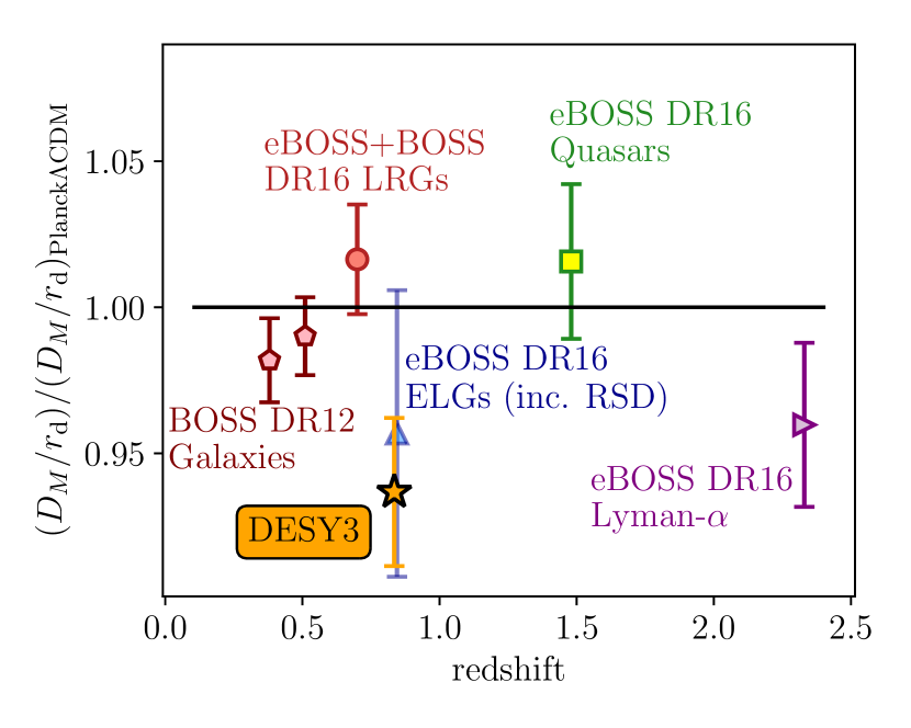
Figure 9: Ratio between the angular diameter distances measured using the BAO feature at different redshifts for several galaxy surveys and the prediction from the cosmological parameters determined by Planck. The DES Y3 measurement is shown by a golden star.

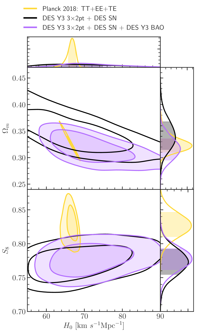
Figure 10: Marginalised constraints in $\Omega_{m}$, $S_{8}$ and $H_{0}$ from different DES datasets: the combination of clustering and lensing (3$\times$2pt), Supernovae (SNe) and BAO. It highlights the degeneracy breaking introduced by BAO enabling to improve constraints on $\Omega_{m}$ and particularly $H_{0}$. The Planck contours are shown in yellow, with $H_{0}$ and $\Omega_{m}$ posteriors being fully consistent, and $S_{8}$ being $\lesssim 1.5\sigma$ low Dark Energy Survey Collaboration et al. (2021).

We now discuss the cosmological implications of our results. Using the Planck cosmology and its measurement of the sound horizon at the drag epoch we can convert our best fit $\alpha$ in Table LABEL:tab:baodata into $D_{M}/r_{\rm d}$ measurements at our effective redshift, see Eq. (22). We obtain $D_{M}/r_{\rm d}=18.92\pm 0.51$ at $z_{\rm eff}=0.835$ from the combination of $w(\theta)$ and $C_{\ell}$ statistics. This represents a fractional error of $2.7\%$, the smallest from any BAO measurement from purely photometric data so far.

Figure 9 displays the comoving angular diameter distance measurement from the DES Y3 BAO sample normalised by the sound horizon scale (golden star) compared to other $D_{M}/r_{\rm d}$ in the literature, and the prediction from Planck $\Lambda$CDM Planck Collaboration et al. (2020) assuming a flat $\Lambda$CDM cosmological model (with fixed neutrino mass). We include measurements from the combined BOSS LOWz + CMASS galaxy samples (at $0.2<z<0.5$ and $0.4<z<0.6$) Alam et al. (2017), from the eBOSS Luminous Red galaxies (LRG, $0.6<z<1.0$) Bautista et al. (2020); Gil-Marín et al. (2020) and the eBOSS Emission Line galaxies (ELG, $0.6<z<1.1$) Tamone et al. (2020); de Mattia et al. (2021), as well as from the eBOSS Quasars ($0.8<z<2.2$) Neveux et al. (2020); Hou et al. (2021) and the Lyman-$\alpha$ combination of auto-correlation and cross-correlation with quasars ($z>2.1$) du Mas des Bourboux et al. (2020). These measurements and their cosmological implications are compiled and discussed in Alam et al. (2017) and Alam et al. (2021), and represent the most updated BAO distance ladder.

The DES Y3 BAO distance measurement is lower than the Planck $\Lambda$CDM prediction by $2.27\sigma$. This value is lower, and represents a more significant difference, than the other BAO measurements in Fig. 9, but is still statistically consistent with Planck. Roughly 1$\sigma$ of this difference is driven by the last redshift bin, as shown in Table LABEL:tab:baodata.

Lastly, we compare with the recent cosmology result from DES Y3 using the combination of clustering and lensing (a.k.a. "DES 3$\times$2pt."), which is based upon the same Y3 GOLD catalogue as this paper. Converting the 3$\times$2pt $\Lambda$CDM Monte Carlo Markov Chains (MCMC) from Dark Energy Survey Collaboration et al. (2021) into a posterior distribution on $D_{M}/r_{\rm d}$ we obtain, $D_{M}(z_{\rm eff}=0.835)/r_{\rm d}=20.139\pm 0.69$ which is bigger than the DES BAO result by about $1.4\sigma$ (accounting for the joint $68\%$ confidence level); while consistent with the Planck result of $D_{M}(z_{\rm eff}=0.835)/r_{\rm d}=20.1$.

The relevance of the DES Y3 BAO measurement for the DES experiment itself is given in Fig. 10, that shows marginalised contours on cosmological parameters assuming flat $\Lambda$CDM from the combinations of DES 3$\times$2pt Dark Energy Survey Collaboration et al. (2021), Supernovae (SNe) Collaboration et al. (2019) and BAO, in addition to Planck Planck Collaboration et al. (2020). Details of the DES likelihoods, scale cuts and priors are detailed in Dark Energy Survey Collaboration et al. (2021); Collaboration et al. (2019) and references therein. DES 3$\times$2pt can constrain well the parameters $\Omega_{m}$ (matter density) and $\sigma_{8}$ (amplitude of density fluctuations), and in particular the combination $S_{8}\equiv\sigma_{8}(\Omega_{m}/0.3)^{2}$, but not the Hubble constant $H_{0}\equiv 100h\,{\rm km~{}s^{-1}}{\rm Mpc}^{-1}$. The constraining power in $\Omega_{m}$ is further increased by the inclusion of DES SNe Collaboration et al. (2019), as discussed in Dark Energy Survey Collaboration et al. (2021). Including a BAO measurement helps constraining the absolute calibration of SNe that propagates to a better measurement of $H_{0}$, in consequence shrinking the ($\Omega_{m},h)$ and $(S_{8},h)$ contours shown in Fig. 10. We obtain for DES 3$\times$2pt + DES SNe,

$$h = 0.691^{+0.138}_{-0.043},$$ (30)

$$\Omega_{m} = 0.344^{+0.029}_{-0.025},$$ (31)

$$S_{8} = 0.773^{+0.018}_{-0.019},$$ (32)

and for DES 3$\times$2pt + DES SNe + DES BAO,

$$h = 0.72^{+0.090}_{-0.053},$$ (33)

$$\Omega_{m} = 0.317^{+0.021}_{-0.020},$$ (34)

$$S_{8} = 0.778^{+0.016}_{-0.017}.$$ (35)

While the central values are consistent, the posterior in $H_{0}$ is made more symmetrical by penalizing low $H_{0}$ values (the prior on $h$ is flat in $0.55-0.91$), with a gain in constraining power of $\sim 20\%$. In turn, the error in $\Omega_{m}$ is reduced by $\sim 26\%$ . The constraining power in $S_{8}$ improves by $\sim 12\%$ with the inclusion of DES BAO.

IX Conclusions

We have measured the ratio of angular diameter distance at an effective redshift $z_{\rm eff}=0.835$ to the physical acoustic scale to be $D_{M}(z_{\rm eff}=0.835)/r_{\rm d}=18.92\pm 0.51$. These results are consistent with the flat $\Lambda$CDM cosmological model to a precision of $2.7\%$. We used clustering measurements from an optimised galaxy sample built upon the first three years of DES data (DES Y3) and described in detail in Carnero Rosell et al. (2021). The sample amounts to 7 million galaxies that cover 4100 deg² on the sky in the redshift range $0.6<z_{\rm photo}<1.1$. This result is consistent with our measurement using 1500 deg² from DES Y1 data Dark Energy Survey Collaboration et al. (2019) using a similarly defined sample, but improves its precision by $\sim 50\%$ due mainly to the area increase.

The measurement was performed in a fully blinded way to avoid any observer confirmation bias. A full battery of quality and consistency tests was defined pre-unblinding and calibrated with a set of 1952 mock realisations of the DES Y3 BAO sample (Ferrero et al., 2021). The analysis choices were fixed using these mocks realiztions as well. Only when the full set of quality and consistency tests was passed by the data we opened the box to see the results.

Two different determinations of the clustering statistics were used to measure the BAO scale: angular correlation function $w(\theta)$ (ACF) and angular power spectrum in spherical harmonics, $C_{\ell}$ (APS). These give very consistent results, as expected from the mock analysis, and presented in Table LABEL:tab:baodata. The error from APS is only marginally worse by $4\%$ to that from ACF. Moreover, the ACF fit yields a $\chi^{2}/{\rm dof}=95.2/89$ corresponding to a $p$-value of 0.3, while the APS yields a $\chi^{2}/{\rm dof}=93.2/99$ corresponding to a $p$-value of 0.6. Thus both represent a good fit to the data and we decided to consider the fiducial DES Y3 result to be the combination of ACF and APS. The BAO feature is detected in the individual and combined likelihoods to a confidence level of more than $3\sigma$.

Our result is lower and in some tension with respect to the prediction from Planck assuming a flat $\Lambda$CDM model, at the level of $2.3\sigma$. Part of this tension originates from our distance measurement at the highest redshift bin, $1.0<z_{\rm photo}<1.1$, both for real and harmonic space. We have checked that the effects on the measurement due to photometric redshifts uncertainties and to the correction of survey properties maps with spatial dependence are very well below the statistical error and have no impact in the final determination. Removing the last bin does not improve the goodness-of-fit of the data or change the fractional errors. Extensive testing with the mocks indicate that the difference in angular diameter distance measurement between the last bin and the ones at lower redshift, while slightly significant, is fully consistent with zero from the statistical point of view given the thresholds that we have defined pre-unblinding. Summarizing, we have verified that the measurement of the BAO scale in the DES Y3 data is robust to all the tests we have performed and is consistent with the simulations.

In addition a number of improvements with respect to our previous analysis have been achieved, most notably

• We developed an end-to-end pipeline to produce mock galaxy catalogues automatically matching input number densities, photometric redshift probabilities ${\rm Prob}(z_{\rm phot},z_{\rm spec})$ and galaxy clustering. The pipeline iteratively populates halo light-cone simulations with galaxies following a Halo Occupation Distribution (HOD) prescription, measures the aforementioned quantities to construct a likelihood, and runs a $\chi^{2}$ minimisation process until it achieves a local minimum. This is fully discussed in Ferrero et al. (2021).

• Contrary to previous work, the damping in the BAO template was derived using non-perturbative analytical expressions following Senatore and Zaldarriaga (2015); Blas et al. (2016). We tested this yields unbiased results on mocks, equivalent to allowing the damping as a free fitting parameter. This enabled us to construct templates for arbitrary cosmologies, without the need to prior mock calibration.

• We have benchmarked with mocks (FLASK, COLA), and finally adopted as default, a halo-model based analytical covariance, CosmoLike Krause and Eifler (2017); Fang et al. (2020a, b). It includes mask effects and higher-order non-gaussian contributions. This enabled us to investigate different assumed cosmologies, besides the one of the mocks.

• We have devised a careful protocol of pre-unblinding checks. From a methodological standpoint, this helps towards converting such protocols in new standards of future BAO analysis.

The BAO angular distance measurement presented in this paper is the most precise measurement in the redshift range $0.6\lesssim z\lesssim 1.1$, and is competitive with other measurements from spectroscopic datasets. Together with results from BOSS galaxies, and eBOSS galaxies, quasars and Lyman-$\alpha$ it helps to construct the most-up-date distance ladder from low to high redshifts ($0.6\lesssim z\lesssim 2.5$). Our results will be revised with the release of the final DES dataset, using approximately the same area but deeper photometry that will likely enable a higher mean redshift.

We expect our work to set the stage and motivate future BAO measurements from much larger imaging datasets, such as those expected from Euclid Laureijs et al. (2011) and LSST LSST Science Collaboration, and others (2009). These should be able to achieve a percentage level fractional errors, and be complementary to results from DESI DESI Collaboration, and others (2016a, b) and Euclid spectroscopy Laureijs et al. (2011).

References

- Riess et al. (1998) A. G. Riess et al., A.J. 116, 1009 (1998), arXiv:astro-ph/9805201 [astro-ph] .
- Perlmutter et al. (1999) S. Perlmutter et al., Astrophys. J. 517, 565 (1999), arXiv:astro-ph/9812133 [astro-ph] .
- Particle Data Group et al. (2020) Particle Data Group et al., Progress of Theoretical and Experimental Physics 2020, 083C01 (2020).
- Weinberg (1989) S. Weinberg, Rev. Mod. Phys. 61, 1 (1989).
- Padmanabhan (2003) T. Padmanabhan, Phys. Rept. 380, 235 (2003), arXiv:hep-th/0212290 .
- Eisenstein et al. (2005) D. J. Eisenstein et al., Astrophys. J. 633, 560 (2005), arXiv:astro-ph/0501171 [astro-ph] .
- Percival et al. (2001) W. J. Percival et al., MNRAS 327, 1297 (2001), arXiv:astro-ph/0105252 [astro-ph] .
- Cole et al. (2005) S. Cole et al., MNRAS 362, 505 (2005), arXiv:astro-ph/0501174 [astro-ph] .
- Percival et al. (2007) W. J. Percival, S. Cole, D. J. Eisenstein, R. C. Nichol, J. A. Peacock, A. C. Pope, and A. S. Szalay, MNRAS 381, 1053 (2007), arXiv:0705.3323 [astro-ph] .
- Gaztañaga et al. (2009) E. Gaztañaga, A. Cabré, and L. Hui, MNRAS 399, 1663 (2009), arXiv:arXiv: 0807.3551 [astro-ph] .
- Percival et al. (2010) W. J. Percival et al., MNRAS 401, 2148 (2010), arXiv:0907.1660 [astro-ph.CO] .
- Ross et al. (2015) A. J. Ross, L. Samushia, C. Howlett, W. J. Percival, A. Burden, and M. Manera, MNRAS 449, 835 (2015), arXiv:1409.3242 [astro-ph.CO] .
- Alam et al. (2017) S. Alam et al., MNRAS 470, 2617 (2017), arXiv:1607.03155 [astro-ph.CO] .
- Ata et al. (2018) M. Ata et al., MNRAS 473, 4773 (2018), arXiv:1705.06373 [astro-ph.CO] .
- Busca et al. (2013) N. G. Busca et al., A&A 552, A96 (2013), arXiv:1211.2616 [astro-ph.CO] .
- Slosar et al. (2013) A. Slosar et al., JCAP 2013, 026 (2013), arXiv:1301.3459 [astro-ph.CO] .
- Font-Ribera et al. (2014) A. Font-Ribera et al., JCAP 2014, 027 (2014), arXiv:1311.1767 [astro-ph.CO] .
- Delubac et al. (2015) T. Delubac et al., A&A 574, A59 (2015), arXiv:1404.1801 [astro-ph.CO] .
- Bautista et al. (2017) J. E. Bautista et al., A&A 603, A12 (2017), arXiv:1702.00176 [astro-ph.CO] .
- du Mas des Bourboux et al. (2020) H. du Mas des Bourboux et al., Astrophys. J. 901, 153 (2020), arXiv:2007.08995 [astro-ph.CO] .
- Alam et al. (2021) S. Alam et al., Phys. Rev. D 103, 083533 (2021), arXiv:2007.08991 [astro-ph.CO] .
- Beutler et al. (2011) F. Beutler et al., MNRAS 416, 3017 (2011), arXiv:1106.3366 [astro-ph.CO] .
- Blake et al. (2011a) C. Blake et al., MNRAS 415, 2892 (2011a), arXiv:1105.2862 [astro-ph.CO] .
- Blake et al. (2011b) C. Blake et al., MNRAS 418, 1707 (2011b), arXiv:1108.2635 [astro-ph.CO] .
- Kazin et al. (2014) E. A. Kazin et al., MNRAS 441, 3524 (2014), arXiv:1401.0358 [astro-ph.CO] .
- Hinton et al. (2017) S. R. Hinton et al., MNRAS 464, 4807 (2017), arXiv:1611.08040 [astro-ph.CO] .
- Flaugher (2005) B. Flaugher, International Journal of Modern Physics A 20, 3121 (2005).
- Dark Energy Survey Collaboration et al. (2016) Dark Energy Survey Collaboration et al., MNRAS 460, 1270 (2016), arXiv:1601.00329 [astro-ph.CO] .
- Dark Energy Survey Collaboration et al. (2019) Dark Energy Survey Collaboration et al., MNRAS 483, 4866 (2019), arXiv:1712.06209 [astro-ph.CO] .
- Padmanabhan et al. (2007) N. Padmanabhan et al., MNRAS 378, 852 (2007), arXiv:astro-ph/0605302 [astro-ph] .
- Estrada et al. (2009) J. Estrada, E. Sefusatti, and J. A. Frieman, Astrophys. J. 692, 265 (2009), arXiv:0801.3485 [astro-ph] .
- Hütsi (2010) G. Hütsi, MNRAS 401, 2477 (2010), arXiv:0910.0492 [astro-ph.CO] .
- Sánchez et al. (2011) E. Sánchez et al., MNRAS 411, 277 (2011), arXiv:1006.3226 [astro-ph.CO] .
- Crocce et al. (2011a) M. Crocce, E. Gaztañaga, A. Cabré, A. Carnero, and E. Sánchez, MNRAS 417, 2577 (2011a), arXiv:1104.5236 [astro-ph.CO] .
- Seo et al. (2012) H.-J. Seo et al., Astrophys. J. 761, 13 (2012), arXiv:1201.2172 [astro-ph.CO] .
- Carnero et al. (2012) A. Carnero, E. Sánchez, M. Crocce, A. Cabré, and E. Gaztañaga, MNRAS 419, 1689 (2012), arXiv:1104.5426 [astro-ph.CO] .
- Sevilla-Noarbe et al. (2021) I. Sevilla-Noarbe et al., ApJS 254, 24 (2021), arXiv:2011.03407 [astro-ph.CO] .
- Carnero Rosell et al. (2021) A. Carnero Rosell et al., To be submitted to MNRAS (2021).
- Crocce et al. (2019) M. Crocce et al. (DES), MNRAS 482, 2807 (2019), arXiv:1712.06211 [astro-ph.CO] .
- Ferrero et al. (2021) I. Ferrero et al., arXiv e-prints , arXiv:2107.04602 (2021), arXiv:2107.04602 [astro-ph.CO] .
- Planck Collaboration et al. (2020) Planck Collaboration et al., A&A 641, A6 (2020), arXiv:1807.06209 [astro-ph.CO] .
- Fosalba et al. (2015a) P. Fosalba, M. Crocce, E. Gaztañaga, and F. J. Castand er, MNRAS 448, 2987 (2015a), arXiv:1312.1707 [astro-ph.CO] .
- Crocce et al. (2015) M. Crocce, F. J. Castander, E. Gaztañaga, P. Fosalba, and J. Carretero, MNRAS 453, 1513 (2015), arXiv:1312.2013 [astro-ph.CO] .
- Fosalba et al. (2015b) P. Fosalba, E. Gaztañaga, F. J. Castander, and M. Crocce, MNRAS 447, 1319 (2015b), arXiv:1312.2947 [astro-ph.CO] .
- Flaugher et al. (2015) B. Flaugher et al., A.J. 150, 150 (2015), arXiv:1504.02900 [astro-ph.IM] .
- Dark Energy Survey Collaboration et al. (2018) Dark Energy Survey Collaboration et al., ApJS 239, 18 (2018), arXiv:1801.03181 [astro-ph.IM] .
- De Vicente et al. (2016) J. De Vicente, E. Sánchez, and I. Sevilla-Noarbe, MNRAS 459, 3078 (2016), arXiv:1511.07623 .
- SDSS Collaboration, (2018) SDSS Collaboration,, ApJS 235, 42 (2018), arXiv:1707.09322 [astro-ph.GA] .
- Childress et al. (2017) M. J. Childress, C. Lidman, T. M. Davis, B. E. Tucker, J. Asorey, F. Yuan, T. M. C. Abbott, F. B. Abdalla, S. Allam, J. Annis, et al., MNRAS 472, 273 (2017), arXiv:1708.04526 [astro-ph.CO] .
- Scodeggio et al. (2018) M. Scodeggio et al., A&A 609, A84 (2018), arXiv:1611.07048 [astro-ph.GA] .
- Guzzo et al. (2014) L. Guzzo et al., A&A 566, A108 (2014), arXiv:1303.2623 [astro-ph.CO] .
- Górski et al. (2005) K. M. Górski, E. Hivon, A. J. Banday, B. D. Wandelt, F. K. Hansen, M. Reinecke, and M. Bartelmann, Astrophys. J. 622, 759 (2005), arXiv:astro-ph/0409513 [astro-ph] .
- Ross et al. (2011) A. J. Ross et al., MNRAS 417, 1350 (2011), arXiv:1105.2320 [astro-ph.CO] .
- Leistedt and Peiris (2014) B. Leistedt and H. V. Peiris, MNRAS 444, 2 (2014), arXiv:1404.6530 [astro-ph.CO] .
- Ross et al. (2017) A. J. Ross et al., MNRAS 464, 1168 (2017), arXiv:1607.03145 [astro-ph.CO] .
- Laurent et al. (2017) P. Laurent et al., JCAP 2017, 017 (2017), arXiv:1705.04718 [astro-ph.CO] .
- Bautista et al. (2018) J. E. Bautista et al., Astrophys. J. 863, 110 (2018), arXiv:1712.08064 [astro-ph.CO] .
- Icaza-Lizaola et al. (2020) M. Icaza-Lizaola et al., MNRAS 492, 4189 (2020), arXiv:1909.07742 [astro-ph.CO] .
- Vakili et al. (2020) M. Vakili et al., arXiv e-prints , arXiv:2008.13154 (2020), arXiv:2008.13154 [astro-ph.CO] .
- Weaverdyck and Huterer (2021) N. Weaverdyck and D. Huterer, MNRAS 503, 5061 (2021), arXiv:2007.14499 [astro-ph.CO] .
- Elvin-Poole et al. (2018) J. Elvin-Poole et al., Phys. Rev. D 98, 042006 (2018), arXiv:1708.01536 [astro-ph.CO] .
- Rodríguez-Monroy et al. (2021) M. Rodríguez-Monroy et al., arXiv e-prints , arXiv:2105.13540 (2021), arXiv:2105.13540 [astro-ph.CO] .
- Izard et al. (2016) A. Izard, M. Crocce, and P. Fosalba, MNRAS 459, 2327 (2016), arXiv:1509.04685 [astro-ph.CO] .
- Tassev et al. (2013) S. Tassev, M. Zaldarriaga, and D. J. Eisenstein, JCAP 2013, 036 (2013), arXiv:1301.0322 [astro-ph.CO] .
- Koda et al. (2016) J. Koda, C. Blake, F. Beutler, E. Kazin, and F. Marin, MNRAS 459, 2118 (2016), arXiv:1507.05329 [astro-ph.CO] .
- Carretero et al. (2015) J. Carretero, F. J. Castander, E. Gaztañaga, M. Crocce, and P. Fosalba, MNRAS 447, 646 (2015), arXiv:1411.3286 [astro-ph.GA] .
- Avila et al. (2018) S. Avila et al., MNRAS 479, 94 (2018), arXiv:1712.06232 [astro-ph.CO] .
- Coles and Jones (1991) P. Coles and B. Jones, MNRAS 248, 1 (1991).
- Clerkin et al. (2017) L. Clerkin et al. (DES), MNRAS 466, 1444 (2017), arXiv:1605.02036 [astro-ph.CO] .
- Xavier et al. (2016) H. S. Xavier, F. B. Abdalla, and B. Joachimi, MNRAS 459, 3693 (2016), arXiv:1602.08503 [astro-ph.CO] .
- Friedrich et al. (2020) O. Friedrich et al., arXiv e-prints , arXiv:2012.08568 (2020), arXiv:2012.08568 [astro-ph.CO] .
- Alonso et al. (2019) D. Alonso, J. Sanchez, A. Slosar, and LSST Dark Energy Science Collaboration, MNRAS 484, 4127 (2019), arXiv:1809.09603 [astro-ph.CO] .
- Jarvis et al. (2004) M. Jarvis, G. Bernstein, and B. Jain, MNRAS 352, 338 (2004), arXiv:astro-ph/0307393 [astro-ph] .
- Krause and Eifler (2017) E. Krause and T. Eifler, MNRAS 470, 2100 (2017), arXiv:1601.05779 [astro-ph.CO] .
- Landy and Szalay (1993) S. D. Landy and A. S. Szalay, Astrophys. J. 412, 64 (1993).
- Alonso (2012) D. Alonso, arXiv e-prints , arXiv:1210.1833 (2012), arXiv:1210.1833 [astro-ph.IM] .
- Hivon et al. (2002) E. Hivon, K. M. Górski, C. B. Netterfield, B. P. Crill, S. Prunet, and F. Hansen, Astrophys. J. 567, 2 (2002), arXiv:astro-ph/0105302 [astro-ph] .
- Nicola et al. (2020) A. Nicola et al., JCAP 2020, 044 (2020), arXiv:1912.08209 [astro-ph.CO] .
- Ross et al. (2017) A. J. Ross et al., MNRAS 472, 4456 (2017), arXiv:1705.05442 [astro-ph.CO] .
- Feldman et al. (1994) H. A. Feldman, N. Kaiser, and J. A. Peacock, Astrophys. J. 426, 23 (1994), arXiv:astro-ph/9304022 [astro-ph] .
- Chan et al. (2021) K. C. Chan, I. Ferrero, S. Avila, A. J. Ross, M. Crocce, and E. Gaztanaga, arXiv e-prints , arXiv:2110.13332 (2021), arXiv:2110.13332 [astro-ph.CO] .
- Chan et al. (2018) K. C. Chan et al., MNRAS 480, 3031 (2018), arXiv:1801.04390 [astro-ph.CO] .
- Senatore and Zaldarriaga (2015) L. Senatore and M. Zaldarriaga, JCAP 2015, 013 (2015), arXiv:1404.5954 [astro-ph.CO] .
- Blas et al. (2016) D. Blas, M. Garny, M. M. Ivanov, and S. Sibiryakov, JCAP 2016, 028 (2016), arXiv:1605.02149 [astro-ph.CO] .
- Lewis et al. (2000) A. Lewis, A. Challinor, and A. Lasenby, Astrophys. J. 538, 473 (2000), arXiv:astro-ph/9911177 [astro-ph] .
- Kaiser (1987) N. Kaiser, MNRAS 227, 1 (1987).
- Krause et al. (2021) E. Krause et al., arXiv e-prints , arXiv:2105.13548 (2021), arXiv:2105.13548 [astro-ph.CO] .
- Vlah et al. (2016) Z. Vlah, U. Seljak, M. Yat Chu, and Y. Feng, JCAP 2016, 057 (2016), arXiv:1509.02120 [astro-ph.CO] .
- Eisenstein and Hu (1998) D. J. Eisenstein and W. Hu, Astrophys. J. 496, 605 (1998), arXiv:astro-ph/9709112 [astro-ph] .
- Ivanov et al. (2020) M. M. Ivanov, M. Simonović, and M. Zaldarriaga, JCAP 2020, 042 (2020), arXiv:1909.05277 [astro-ph.CO] .
- Ivanov and Sibiryakov (2018) M. M. Ivanov and S. Sibiryakov, JCAP 2018, 053 (2018), arXiv:1804.05080 [astro-ph.CO] .
- Crocce et al. (2011b) M. Crocce, A. Cabré, and E. Gaztañaga, MNRAS 414, 329 (2011b), arXiv:1004.4640 [astro-ph.CO] .
- Takada and Jain (2009) M. Takada and B. Jain, MNRAS 395, 2065 (2009), arXiv:0810.4170 [astro-ph] .
- Takada and Hu (2013) M. Takada and W. Hu, Phys. Rev. D 87, 123504 (2013), arXiv:1302.6994 [astro-ph.CO] .
- Fang et al. (2020a) X. Fang, T. Eifler, and E. Krause, MNRAS 497, 2699 (2020a), arXiv:2004.04833 [astro-ph.CO] .
- Fang et al. (2020b) X. Fang, E. Krause, T. Eifler, and N. MacCrann, JCAP 2020, 010 (2020b), arXiv:1911.11947 [astro-ph.CO] .
- Troxel et al. (2018) M. A. Troxel, E. Krause, C. Chang, T. F. Eifler, O. Friedrich, D. Gruen, N. MacCrann, et al., MNRAS 479, 4998 (2018), arXiv:1804.10663 [astro-ph.CO] .
- Efstathiou (2004) G. Efstathiou, MNRAS 349, 603 (2004), arXiv:astro-ph/0307515 [astro-ph] .
- García-García et al. (2019) C. García-García, D. Alonso, and E. Bellini, JCAP 2019, 043 (2019), arXiv:1906.11765 [astro-ph.CO] .
- Cuceu et al. (2020) A. Cuceu, A. Font-Ribera, and B. Joachimi, JCAP 2020, 035 (2020), arXiv:2004.02761 [astro-ph.CO] .
- Camacho et al. (2019) H. Camacho et al. (DES), MNRAS 487, 3870 (2019), arXiv:1807.10163 [astro-ph.CO] .
- Crocce and Scoccimarro (2008) M. Crocce and R. Scoccimarro, Phys. Rev. D 77, 023533 (2008), arXiv:0704.2783 .
- Padmanabhan and White (2009) N. Padmanabhan and M. White, Phys. Rev. D 80, 063508 (2009), arXiv:0906.1198 [astro-ph.CO] .
- Dark Energy Survey Collaboration et al. (2021) Dark Energy Survey Collaboration et al., arXiv e-prints , arXiv:2105.13549 (2021), arXiv:2105.13549 [astro-ph.CO] .
- Bautista et al. (2020) J. E. Bautista et al., MNRAS 500, 736 (2020), arXiv:2007.08993 [astro-ph.CO] .
- Gil-Marín et al. (2020) H. Gil-Marín et al., MNRAS 498, 2492 (2020), arXiv:2007.08994 [astro-ph.CO] .
- Tamone et al. (2020) A. Tamone et al., MNRAS 499, 5527 (2020), arXiv:2007.09009 [astro-ph.CO] .
- de Mattia et al. (2021) A. de Mattia et al., MNRAS 501, 5616 (2021), arXiv:2007.09008 [astro-ph.CO] .
- Neveux et al. (2020) R. Neveux et al., MNRAS 499, 210 (2020), arXiv:2007.08999 [astro-ph.CO] .
- Hou et al. (2021) J. Hou et al., MNRAS 500, 1201 (2021), arXiv:2007.08998 [astro-ph.CO] .
- Collaboration et al. (2019) D. E. S. Collaboration et al., ApJ 872, L30 (2019), arXiv:1811.02374 [astro-ph.CO] .
- Laureijs et al. (2011) R. Laureijs et al., arXiv e-prints , arXiv:1110.3193 (2011), arXiv:1110.3193 [astro-ph.CO] .
- LSST Science Collaboration, and others (2009) LSST Science Collaboration, and others, arXiv e-prints , arXiv:0912.0201 (2009), arXiv:0912.0201 [astro-ph.IM] .
- DESI Collaboration, and others (2016a) DESI Collaboration, and others, arXiv e-prints , arXiv:1611.00036 (2016a), arXiv:1611.00036 [astro-ph.IM] .
- DESI Collaboration, and others (2016b) DESI Collaboration, and others, arXiv e-prints , arXiv:1611.00037 (2016b), arXiv:1611.00037 [astro-ph.IM] .