The Bayesian Learning Rule

\nameMohammad Emtiyaz Khan \emailemtiyaz.khan@riken.jp
\addrRIKEN Center for Advanced Intelligence Project
1-4-1 Nihonbashi, Chuo-ku, Tokyo 103-0027, Japan \AND\nameHåvard Rue \emailhaavard.rue@kaust.edu.sa
\addrCEMSE Division
King Abdullah University of Science and Technology
Thuwal 23955-6900, Saudi Arabia
Abstract

We show that many machine-learning algorithms are specific instances of a single algorithm called the Bayesian learning rule. The rule, derived from Bayesian principles, yields a wide-range of algorithms from fields such as optimization, deep learning, and graphical models. This includes classical algorithms such as ridge regression, Newton’s method, and Kalman filter, as well as modern deep-learning algorithms such as stochastic-gradient descent, RMSprop, and Dropout. The key idea in deriving such algorithms is to approximate the posterior using candidate distributions estimated by using natural gradients. Different candidate distributions result in different algorithms and further approximations to natural gradients give rise to variants of those algorithms. Our work not only unifies, generalizes, and improves existing algorithms, but also helps us design new ones.

Keywords: Bayesian methods, optimization, deep learning, graphical models.

1 Introduction

1.1 Learning-algorithms

Machine Learning (ML) methods have been extremely successful in solving many challenging problems in fields such as computer vision, natural-language processing and artificial intelligence (AI). The main idea is to formulate those problems as prediction problems, and learn a model on existing data to predict the future outcomes. For example, to design an AI agent that can recognize objects in an image, we can collect a dataset with $N$ images $\text{$\boldsymbol{x}$}_{i}\in{}^{D}$ and object labels $y_{i}\in\{1,2,\ldots,K\}$, and learn a model $f_{\text{\text{$\boldsymbol{\theta}$}}}(\text{$\boldsymbol{x}$})$ with parameters $\text{$\boldsymbol{\theta}$}\in{}^{P}$ to predict the label for a new image. Learning algorithms are often employed to estimate $\boldsymbol{\theta}$ using the principle of trial-and-error, for example, by using Empirical Risk Minimization (ERM),

$$\text{$\boldsymbol{\theta}$}_{*}=\arg\min_{\text{\text{$\boldsymbol{\theta}$}}}\bar{\ell}(\text{$\boldsymbol{\theta}$})\quad\text{where}\quad\bar{\ell}(\text{$\boldsymbol{\theta}$})=\sum_{i=1}^{N}\ell(y_{i},f_{\text{\text{$\boldsymbol{\theta}$}}}(\text{$\boldsymbol{x}$}_{i}))+R(\text{$\boldsymbol{\theta}$}).$$ (1)

Here, $\ell(y,f_{\text{\text{$\boldsymbol{\theta}$}}}(\text{$\boldsymbol{x}$}))$ is a loss function that encourages the model to predict well and ${R}(\text{$\boldsymbol{\theta}$})$ is a regularizer that prevents it from overfitting. A wide-variety of such learning-algorithms exist in the literature to solve a variety of learning problems, for example, ridge regression, Kalman filters, gradient descent, and Newton’s method. These algorithms play a key role in the success of modern ML.

Learning-algorithms are often derived by borrowing and combining ideas from a diverse set of fields, such as statistics, optimization, and computer science. For example, the field of probabilistic graphical models (Koller and Friedman, 2009; Bishop, 2006) uses popular algorithms such as ridge-regression (Hoerl and Kennard, 1970), Kalman filters (Kalman, 1960), the Viterbi algorithm for Hidden Markov Models (Stratonovich, 1965), and Expectation-Maximization (EM) (Dempster et al., 1977). The field of approximate inference builds upon such algorithms to perform inference on complex graphical models, for example, algorithms such as Laplace’s method (Laplace, 1986; Tierney and Kadane, 1986; Rue and Martino, 2007; Rue et al., 2009, 2017), stochastic variational inference (SVI) (Hoffman et al., 2013; Sato, 2001), Variational message passing (VMP) (Winn and Bishop, 2005) etc. Similarly, the field of continuous optimization has its own popular methods such as gradient descent (Cauchy, 1847), Newton’s method, and mirror descent (Nemirovski and Yudin, 1978), and deep-learning (DL) methods use them to design new techniques that work with massive models and datasets, for example, stochastic-gradient descent (Robbins and Monro, 1951), RMSprop (Tieleman and Hinton, 2012), Adam (Kingma and Ba, 2015), Dropout regularization (Srivastava et al., 2014), and Straight-Through Estimator (STE) (Bengio et al., 2013). Such mixing of algorithms from diverse fields is a strength of the ML community, and our goal here is to provide common principles to unify, generalize, and improve such algorithms.

1.2 The Bayesian learning rule

We show that a wide-range of well-known learning-algorithms from a variety of fields are all specific instances of a single learning algorithm derived from Bayesian principles. The starting point is to extend Eq. 1 by using the variational formulation of Zellner (1988), where we optimize over a well-defined candidate distribution $q(\text{$\boldsymbol{\theta}$})$, and for which the minimizer

$$q_{*}(\text{$\boldsymbol{\theta}$})=\operatorname*{arg\,min}_{q(\text{\text{$\boldsymbol{\theta}$}})}\,\,\mathbb{E}_{q}\left[\sum_{i=1}^{N}\ell(y_{i},f_{\text{\text{$\boldsymbol{\theta}$}}}(\text{$\boldsymbol{x}$}_{i}))\right]+\mathbb{D}_{KL}[q(\text{$\boldsymbol{\theta}$})\,\|\,p(\text{$\boldsymbol{\theta}$})]$$ (2)

defines a generalized posterior (Zhang, 1999; Catoni, 2007; Bissiri et al., 2016) in lack of a precise likelihood. We can rewrite the objective in terms of entropy $\mathcal{H}(q)=\mathbb{E}_{q}[-\log q(\text{$\boldsymbol{\theta}$})]$ by expanding the Kullback-Leibler Divergence (KLD) as follows,

$$\mathbb{D}_{KL}[q(\text{$\boldsymbol{\theta}$})\,\|\,p(\text{$\boldsymbol{\theta}$})]=\mathbb{E}_{q}\left[\log\frac{q(\text{$\boldsymbol{\theta}$})}{p(\text{$\boldsymbol{\theta}$})}\right]=\mathbb{E}_{q}\left[R(\text{$\boldsymbol{\theta}$})\right]-\mathcal{H}(q),$$

where we chose the prior to be $p(\text{$\boldsymbol{\theta}$})\propto\exp(-R(\text{$\boldsymbol{\theta}$}))$. Plugging this in Eq. 2, we get

$$q_{*}(\text{$\boldsymbol{\theta}$})=\operatorname*{arg\,min}_{q(\text{\text{$\boldsymbol{\theta}$}})}\,\,\mathbb{E}_{q}\left(\bar{\ell}(\text{$\boldsymbol{\theta}$})\right)-\mathcal{H}(q).$$

When $\exp(-\ell(y_{i},f_{\text{\text{$\boldsymbol{\theta}$}}}(\text{$\boldsymbol{x}$}_{i})))$ is proportional to the likelihood of $y_{i}$ for all $i$, then $q_{*}(\text{$\boldsymbol{\theta}$})$ is the posterior distribution (Zellner, 1988); see App. A for a proof.

We use two components to derive learning algorithms from this Bayesian formulation,

  1. 1.

    A (sub-)class of distributions ${\mathcal{Q}}$ to optimize over. In our discussion, we will assume ${\mathcal{Q}}$ to be the set of a regular and minimal exponential family

    $$q_{\text{$\boldsymbol{\lambda}$}}(\text{$\boldsymbol{\theta}$})=h(\text{$\boldsymbol{\theta}$})\exp\left[\langle\text{$\boldsymbol{\lambda}$},\text{$\boldsymbol{T}$}(\text{$\boldsymbol{\theta}$})\rangle-A(\text{$\boldsymbol{\lambda}$})\right],$$

    where $\text{$\boldsymbol{\lambda}$}\in\Omega\subset{}^{M}$ are the natural (or canonical) parameter in a non-empty open set $\Omega$. The cumulant (or log partition) function $A(\text{$\boldsymbol{\lambda}$})$ is finite, strictly convex and differentiable over $\Omega$. Further, $\text{$\boldsymbol{T}$}(\text{$\boldsymbol{\theta}$})$ is the sufficient statistics, $\langle\cdot,\cdot\rangle$ is an inner product and $h(\text{$\boldsymbol{\theta}$})$ is the base measure. The expectation parameter $\text{$\boldsymbol{\mu}$}(\text{$\boldsymbol{\lambda}$})=\mathbb{E}_{q_{\text{$\boldsymbol{\lambda}$}}}[\text{$\boldsymbol{T}$}(\text{$\boldsymbol{\theta}$})]\in\mathcal{M}$ is a (bijective) function of $\boldsymbol{\lambda}$. Examples later will include the multivariate Normal distribution and the Bernoulli distribution (see Table 2 for a list).

  2. 2.

    An optimizing algorithm, called the Bayesian learning rule (BLR), that locates the best candidate $q_{\text{$\boldsymbol{\lambda}$}_{*}}(\text{$\boldsymbol{\theta}$})$ in ${\mathcal{Q}}$, by updating the candidate $q_{\text{$\boldsymbol{\lambda}$}_{t}}(\text{$\boldsymbol{\theta}$})$ with natural parameter $\text{$\boldsymbol{\lambda}$}_{t}$ at iteration $t$ using a sequence of learning rates $\rho_{t}>0$:

    $$\text{$\boldsymbol{\lambda}$}_{t+1}\leftarrow\text{$\boldsymbol{\lambda}$}_{t}-\rho_{t}\widetilde{\nabla}_{\text{$\boldsymbol{\lambda}$}}\left[\mathbb{E}_{q_{\text{$\boldsymbol{\lambda}$}_{t}}}\left(\bar{\ell}(\text{$\boldsymbol{\theta}$})\right)-\mathcal{H}(q_{t})\right].$$ (3)

    The updates use the natural-gradients (Amari, 1998), denoted by $\widetilde{\nabla}_{\text{$\boldsymbol{\lambda}$}}$, and defined as

    $$\widetilde{\nabla}_{\text{$\boldsymbol{\lambda}$}}\mathbb{E}_{q_{\text{$\boldsymbol{\lambda}$}_{t}}}(\cdot)=\text{$\boldsymbol{F}$}(\text{$\boldsymbol{\lambda}$}_{t})^{-1}\,\left[\left.\nabla_{\text{$\boldsymbol{\lambda}$}}\mathbb{E}_{q_{\text{$\boldsymbol{\lambda}$}}}(\cdot)\right|_{\text{\text{$\boldsymbol{\lambda}$}}=\text{\text{$\boldsymbol{\lambda}$}}_{t}}\right]\,\,=\,\,\left.\nabla_{\text{$\boldsymbol{\mu}$}}\mathbb{E}_{q_{\text{$\boldsymbol{\lambda}$}}}(\cdot)\right|_{\text{$\boldsymbol{\mu}$}=\nabla_{\text{$\boldsymbol{\lambda}$}}A(\text{$\boldsymbol{\lambda}$}_{t})},$$ (4)

    which rescale the vanilla gradients $\nabla_{\text{$\boldsymbol{\lambda}$}}$ with the Fisher information matrix (FIM) $\text{$\boldsymbol{F}$}(\text{$\boldsymbol{\lambda}$})=\nabla_{\text{$\boldsymbol{\lambda}$}}^{2}A(\text{$\boldsymbol{\lambda}$})$ to adjust for the geometry in the natural-parameter space $\Omega$. The second equality follows from the chain rule to express natural-gradients as vanilla gradients with respect to $\text{$\boldsymbol{\mu}$}=\nabla_{\text{$\boldsymbol{\lambda}$}}A(\text{$\boldsymbol{\lambda}$})$ (Malagò et al., 2011; Raskutti and Mukherjee, 2015). Throughout, we will use this property to simplify natural-gradient computations. These details are discussed in Sec. 2, where we show that the BLR update can also be seen as a mirror descent algorithm, where the geometry of the Bregman divergence is dictated by the chosen exponential-family. Throughout, we will assume $\text{$\boldsymbol{\lambda}$}_{t}\in\Omega$ for all $t$, which in practice might require a line-search or a projection step.

The main message of this paper is that many well-known learning-algorithms – such as those used in optimization, deep learning, and machine learning in general – can be derived directly following the above scheme via a single algorithm (BLR) that optimizes Eq. 2. Different exponential families ${\mathcal{Q}}$ give rise to different algorithms, and within those, various approximations to natural-gradients that are needed, give rise to many variants. These results are extended to mixture-candidates in Sec. 3.2, and we expect them to hold in general for other classes of candidate distributions.

Our use of natural-gradients here is not a matter of choice. In fact, natural-gradients are inherently present in all solutions of the Bayesian objective in Eq. 2. For example, the natural parameter $\text{$\boldsymbol{\lambda}$}_{*}$ of a solution $q_{\text{$\boldsymbol{\lambda}$}_{*}}(\text{$\boldsymbol{\theta}$})$ is a fixed point of Eq. 3, and at convergence

$$\begin{split}\text{$\boldsymbol{\lambda}$}_{*}=\text{$\boldsymbol{\lambda}$}_{*}-\rho_{*}\widetilde{\nabla}_{\text{$\boldsymbol{\lambda}$}}\left[\mathbb{E}_{q_{\text{$\boldsymbol{\lambda}$}_{*}}}\left[\bar{\ell}(\text{$\boldsymbol{\theta}$})\right]-\mathcal{H}(q_{\text{$\boldsymbol{\lambda}$}_{*}})\right]&\implies\text{$\boldsymbol{\lambda}$}_{*}=\widetilde{\nabla}_{\text{$\boldsymbol{\lambda}$}}\mathbb{E}_{q_{\text{$\boldsymbol{\lambda}$}_{*}}}\left[-\bar{\ell}(\text{$\boldsymbol{\theta}$})\right].\end{split}$$ (5)

In the second equality, we assume that the base-measure $h(\text{$\boldsymbol{\theta}$})$ is a constant, so that $\widetilde{\nabla}_{\text{$\boldsymbol{\lambda}$}}\mathcal{H}(q_{\text{$\boldsymbol{\lambda}$}})=-\text{$\boldsymbol{\lambda}$}$ (see App. B). The equality states that the natural parameter $\text{$\boldsymbol{\lambda}$}_{*}$ must be equal to the natural gradient of $\mathbb{E}_{q_{\text{$\boldsymbol{\lambda}$}_{*}}}\left[-\bar{\ell}(\text{$\boldsymbol{\theta}$})\right]$, therefore estimation of $q_{\text{$\boldsymbol{\lambda}$}_{*}}(\text{$\boldsymbol{\theta}$})$ is tightly coupled to computation of natural gradients. Depite this, the importance of natural-gradients is entirely missed in the Bayesian/variational inference literature, including textbooks, reviews, tutorials on this topic (Bishop, 2006; Murphy, 2012; Blei et al., 2017; Zhang et al., 2018a) where natural-gradients are often put in a special category. Our work fixes this issue.

We will show that natural gradients retrieve essential higher-order information about the loss landscape which are then assigned to appropriate natural parameters using Eq. 5. The information-matching is due to the presence of the entropy term there, which is an important quantity for the optimality of Bayes in general (Jaynes, 1982; Zellner, 1988) and generally absent in non-Bayesian formulations, for instance, Eq. 1. The entropy term in general leads to exponential-weighting in Bayes’ rule (Littlestone and Warmuth, 1994; Vovk, 1990). In our context, it gives rise to natural-gradients and, as we will soon see, automatically determines the complexity of the derived algorithm through the complexity of the class of distributions $\mathcal{Q}$, yielding a principled way to develop new algorithms.

Overall, our work demonstrates the importance of natural-gradients and information geometry for algorithm design in ML. This is similar in spirit to Information Geometric Optimization (Ollivier et al., 2017) which focuses on the optimization of black-box, deterministic functions. In contrast, we derive generic learning algorithms by using a Bayesian objective where an additional entropy term is added.

The BLR we use is a generalization of the method by Khan and Lin (2017); Khan and Nielsen (2018), proposed specifically for variational inference. Here, we establish it as a general learning rule to derive many old and new learning algorithms. These include both Bayesian and non-Bayesian algorithms, going way beyond its original proposal. We do not claim that these successful algorithms work well because they are derived from the BLR. Rather, we use the BLR to simply unravel the inherent Bayesian nature of these “good” algorithms. In this sense, the BLR can be seen as a variant of Bayes’ rule, useful for generic algorithm design.

1.3 Examples

To fix ideas, we will now use the BLR to derive three classical algorithms: gradient descent, Newton’s method, and ridge regression. Such derivations are repeated throughout the paper to recover various algorithms in different fields. A full list of the learning algorithms derived in this paper is given in Table 1. We not only unify and generalize existing algorithms but also derive new ones. These includes: (i) a new multimodal optimization algorithm, (ii) new uncertainty estimation algorithms (OGN and VOGN), (iii) the BayesBiNN algorithm for binary neural networks, and (iv) non-conjugate variational inference algorithms.

For notational simplicity, we will write $q_{\text{$\boldsymbol{\lambda}$}_{t}}$ as $q_{t}$ in the rest of the paper. Throughout this section, we choose $\mathcal{Q}$ to be the set of multivariate Gaussians and use the following simplified form of the BLR,

$$\text{$\boldsymbol{\lambda}$}_{t+1}\leftarrow(1-\rho_{t})\text{$\boldsymbol{\lambda}$}_{t}-\rho_{t}\nabla_{\text{$\boldsymbol{\mu}$}}\mathbb{E}_{q_{t}}\left[\bar{\ell}(\text{$\boldsymbol{\theta}$})+\log h(\text{$\boldsymbol{\theta}$})\right],$$ (6)

This is obtained by using $\nabla_{\text{$\boldsymbol{\mu}$}}\mathcal{H}(q)=-\text{$\boldsymbol{\lambda}$}-\nabla_{\text{$\boldsymbol{\mu}$}}\mathbb{E}_{q}(\log h(\text{$\boldsymbol{\theta}$}))$; see the derivation in App. B.

1.3.1 Gradient descent

The gradient descent algorithm uses the following update

$$\text{$\boldsymbol{\theta}$}_{t+1}\leftarrow\text{$\boldsymbol{\theta}$}_{t}-\rho_{t}\nabla_{\text{\text{$\boldsymbol{\theta}$}}}\bar{\ell}(\text{$\boldsymbol{\theta}$}_{t}),$$

using only the first-order information $\nabla_{\text{\text{$\boldsymbol{\theta}$}}}\bar{\ell}(\text{$\boldsymbol{\theta}$}_{t})$ (the gradient evaluated at $\text{$\boldsymbol{\theta}$}_{t}$). We choose $q(\text{$\boldsymbol{\theta}$})=\text{${\cal N}$}(\text{$\boldsymbol{\theta}$}|\text{$\boldsymbol{m}$},\text{$\boldsymbol{I}$})$, a multivariate Gaussian with unknown mean $\boldsymbol{m}$ and known covariance matrix set to $\boldsymbol{I}$ for simplicity; a more general case is given in Eq. 35.

We can now simply plug in the definition of $\text{$\boldsymbol{\lambda}$},\text{$\boldsymbol{\mu}$},$ and $h(\text{$\boldsymbol{\theta}$})$ in Eq. 6. For $q(\text{$\boldsymbol{\theta}$})=\text{${\cal N}$}(\text{$\boldsymbol{\theta}$}|\text{$\boldsymbol{m}$},\text{$\boldsymbol{I}$})$, we have $\text{$\boldsymbol{\lambda}$}=\text{$\boldsymbol{\mu}$}=\text{$\boldsymbol{m}$}$ (Table 2). The log of the base measure is $\log h(\text{$\boldsymbol{\theta}$})=-\text{$\frac{1}{2}$}P\log(2\pi)-\text{$\frac{1}{2}$}\text{$\boldsymbol{\theta}$}^{T}\text{$\boldsymbol{\theta}$}$. Using these in Eq. 6, the update follows directly:

$\displaystyle\text{$\boldsymbol{m}$}_{t+1}\leftarrow\text{$\boldsymbol{m}$}_{t}-\rho_{t}\left.\nabla_{\text{\text{$\boldsymbol{m}$}}}\mathbb{E}_{\text{\text{${\cal N}$}}(\text{\text{$\boldsymbol{\theta}$}}|\text{\text{$\boldsymbol{m}$}},\text{$\boldsymbol{I}$})}\left[\bar{\ell}(\text{$\boldsymbol{\theta}$})\right]\right|_{\text{\text{$\boldsymbol{m}$}}=\text{\text{$\boldsymbol{m}$}}_{t}}.$ (7)

This is gradient descent but over the expected loss $\mathbb{E}_{q}\left[\bar{\ell}(\text{$\boldsymbol{\theta}$})\right]$. We can remove the expectation by using the first-order delta method (Dorfman, 1938; Ver Hoef, 2012) (App. C) where we approximate the expectation of a function by its value at the mean,

$$\nabla_{\text{$\boldsymbol{m}$}}\mathbb{E}_{q}\left[\bar{\ell}(\text{$\boldsymbol{\theta}$})\right]\approx\left.\nabla_{\text{$\boldsymbol{\theta}$}}\bar{\ell}(\text{$\boldsymbol{\theta}$})\right|_{\text{$\boldsymbol{\theta}$}=\text{\text{$\boldsymbol{m}$}}}.$$

With this, the BLR equals the gradient descent algorithm with $\text{$\boldsymbol{m}$}_{t}$ as the iterate $\text{$\boldsymbol{\theta}$}_{t}$. The two choices, first of the distribution $\mathcal{Q}$ and second of the delta method, give us gradient descent from the BLR.

The delta method allows us to interpret non-Bayesian solutions as crude approximations of Bayesian ones. By approximating the expectation in the BLR with a greedy approximation, we are back to minimizing a deterministic (non-Bayesian) objective. This observation suggests that Eq. 7 should perform better than gradient descent. In Sec. 4.4, we will revisit this point and see that averaging in fact leads to improved uncertainty and better robustness properties. Using the Dirac’s-delta distribution instead of the delta method is not advisable, as their use in this context is fundamentally flawed. This is because the entropy goes to $-\infty$, making the Bayesian objective meaningless (Welling et al., 2008).

1.3.2 Newton’s method

Newton’s method is a second-order method

$\displaystyle\text{$\boldsymbol{\theta}$}_{t+1}\leftarrow\text{$\boldsymbol{\theta}$}_{t}-\left[\nabla_{\text{\text{$\boldsymbol{\theta}$}}}^{2}\bar{\ell}(\text{$\boldsymbol{\theta}$}_{t})\right]^{-1}\left[\nabla_{\text{\text{$\boldsymbol{\theta}$}}}\bar{\ell}(\text{$\boldsymbol{\theta}$}_{t})\right].$ (8)

which too can be derived from the BLR by expanding the class $\mathcal{Q}$ to $q(\text{$\boldsymbol{\theta}$})=\text{${\cal N}$}(\text{$\boldsymbol{\theta}$}|\text{$\boldsymbol{m}$},\text{$\boldsymbol{S}$}^{-1})$ with an unknown precision matrix $\boldsymbol{S}$. This example illustrates a property of the BLR: the complexity of the derived algorithm is directly related to the complexity of the exponential family ${\mathcal{Q}}$. Fixed covariances previously gave rise to gradient-descent (a first-order method) and by increasing the complexity where we also learn the precision matrix, the BLR reduces to a (more complex) second-order method.

We use the simplified form of the BLR given in Eq. 6. The base measure is a constant, and the natural and expectation parameters divide themselves into natural pairs

$$\begin{array}[]{llll}\begin{array}[]{cc}\text{$\boldsymbol{\lambda}$}^{(1)}&=\text{$\boldsymbol{S}$}\text{$\boldsymbol{m}$},\\ \text{$\boldsymbol{\lambda}$}^{(2)}&=-\text{$\frac{1}{2}$}\text{$\boldsymbol{S}$},\end{array}&\quad\begin{array}[]{lll}\text{$\boldsymbol{\mu}$}^{(1)}&=\mathbb{E}_{q}[\text{$\boldsymbol{\theta}$}]&=\text{$\boldsymbol{m}$},\\ \text{$\boldsymbol{\mu}$}^{(2)}&=\mathbb{E}_{q}[\text{$\boldsymbol{\theta}$}\text{$\boldsymbol{\theta}$}^{\top}]&=\text{$\boldsymbol{S}$}^{-1}+\text{$\boldsymbol{m}$}\text{$\boldsymbol{m}$}^{T}.\\ \end{array}\end{array}$$ (9)

The natural gradients can be expressed in terms of the gradient and Hessian of $\bar{\ell}(\text{$\boldsymbol{\theta}$})$. To show this, we use the chain-rule to first write gradients with respect to $\boldsymbol{\mu}$ in terms of $(\text{$\boldsymbol{m}$},\text{$\boldsymbol{S}$}^{-1})$ (first equality below) and then use Bonnet’s and Price’s theorem respectively (Bonnet, 1964; Price, 1958; Rezende et al., 2014) to get the second equality (full derivation is in App. D),

$\displaystyle\nabla_{\text{$\boldsymbol{\mu}$}^{(1)}}\mathbb{E}_{q}[\bar{\ell}(\text{$\boldsymbol{\theta}$})]$ $\displaystyle=\nabla_{\boldsymbol{\mathbf{m}}}\mathbb{E}_{q}[\bar{\ell}(\text{$\boldsymbol{\theta}$})]-2\left[\nabla_{\mathbf{S}^{-1}}\mathbb{E}_{q}[\bar{\ell}(\text{$\boldsymbol{\theta}$})]\right]\text{$\boldsymbol{m}$}$ $\displaystyle=\mathbb{E}_{q}[\nabla_{\boldsymbol{\theta}}\bar{\ell}(\text{$\boldsymbol{\theta}$})]-\mathbb{E}_{q}[\nabla_{\boldsymbol{\theta}}^{2}\bar{\ell}(\text{$\boldsymbol{\theta}$})]\text{$\boldsymbol{m}$},$ (10)
$\displaystyle\nabla_{\text{$\boldsymbol{\mu}$}^{(2)}}\mathbb{E}_{q}[\bar{\ell}(\text{$\boldsymbol{\theta}$})]$ $\displaystyle=\nabla_{\mathbf{S}^{-1}}\mathbb{E}_{q}[\bar{\ell}(\text{$\boldsymbol{\theta}$})]$ $\displaystyle=\text{$\frac{1}{2}$}\mathbb{E}_{q}[\nabla_{\boldsymbol{\theta}}^{2}\bar{\ell}(\text{$\boldsymbol{\theta}$})].$ (11)

The expressions show that the natural gradients contain the information about the first and second-order derivatives of $\bar{\ell}(\text{$\boldsymbol{\theta}$})$.

The BLR now turns into an online variant of Newton’s method where the precision matrix contains an exponential-smoothed Hessian average, used as a pre-conditioner to update the mean,

$\displaystyle\text{$\boldsymbol{m}$}_{t+1}\leftarrow\text{$\boldsymbol{m}$}_{t}-\rho_{t}\text{$\boldsymbol{S}$}_{t+1}^{-1}\mathbb{E}_{q_{t}}\left[\nabla_{\text{\text{$\boldsymbol{\theta}$}}}\bar{\ell}(\text{$\boldsymbol{\theta}$})\right]\quad\text{and}\quad\text{$\boldsymbol{S}$}_{t+1}\leftarrow(1-\rho_{t})\text{$\boldsymbol{S}$}_{t}+\rho_{t}\mathbb{E}_{q_{t}}\left[\nabla_{\text{\text{$\boldsymbol{\theta}$}}}^{2}\bar{\ell}(\text{$\boldsymbol{\theta}$})\right].$ (12)

We can recover the classical Newton’s method in three steps. First, apply the delta method (see Eqs. 65 and 66 in App. C),

$$\mathbb{E}_{q}\left[\nabla_{\text{\text{$\boldsymbol{\theta}$}}}\bar{\ell}(\text{$\boldsymbol{\theta}$})\right]\approx\left.\nabla_{\text{$\boldsymbol{\theta}$}}\bar{\ell}(\text{$\boldsymbol{\theta}$})\right|_{\text{$\boldsymbol{\theta}$}=\text{$\boldsymbol{m}$}}\quad\text{and}\quad\mathbb{E}_{q}\left[\nabla_{\text{\text{$\boldsymbol{\theta}$}}}^{2}\bar{\ell}(\text{$\boldsymbol{\theta}$})\right]\approx\left.\nabla^{2}_{\text{$\boldsymbol{\theta}$}}\bar{\ell}(\text{$\boldsymbol{\theta}$})\right|_{\text{$\boldsymbol{\theta}$}=\text{$\boldsymbol{m}$}}.$$ (13)

Second, set the learning rate to 1 which is justified when the loss is strongly convex or the algorithm is initialized close to the solution. Finally, treat the mean $\text{$\boldsymbol{m}$}_{t}$ as the iterate $\text{$\boldsymbol{\theta}$}_{t}$.

1.3.3 Ridge regression

Why do we get a second-order method when we increase the complexity of the Gaussian? This is due to the natural gradients which, depending on the complexity of the distribution, retrieve essential higher-order information about the loss landscape. We illustrate this now through the simplest non-trivial case of Ridge regression. Denote input matrix by $\text{$\boldsymbol{X}$}\in{}^{N\times D}$ and output by $\text{$\boldsymbol{y}$}\in{}^{N}$. The loss is quadratic: $\bar{\ell}(\text{$\boldsymbol{\theta}$})=\text{$\frac{1}{2}$}(\text{$\boldsymbol{y}$}-\text{$\boldsymbol{X}$}\text{$\boldsymbol{\theta}$})^{\top}(\text{$\boldsymbol{y}$}-\text{$\boldsymbol{X}$}\text{$\boldsymbol{\theta}$})+\text{$\frac{1}{2}$}\delta\text{$\boldsymbol{\theta}$}^{\top}\text{$\boldsymbol{\theta}$}$ with $\delta>0$ as the regularization parameter, and the solution is available in closed-form:

$$\text{$\boldsymbol{\theta}$}_{*}=(\text{$\boldsymbol{X}$}^{\top}\text{$\boldsymbol{X}$}+\delta\text{$\boldsymbol{I}$})^{-1}\text{$\boldsymbol{X}$}^{\top}\text{$\boldsymbol{y}$}.$$

Natural gradients for this case are extremely easy to derive. We first note that the expected-loss is linear in $\boldsymbol{\mu}$, that is,

$$\mathbb{E}_{q}\left[\bar{\ell}(\text{$\boldsymbol{\theta}$})\right]=-\text{$\boldsymbol{y}$}^{\top}\text{$\boldsymbol{X}$}\text{$\boldsymbol{\mu}$}^{(1)}+\text{Tr}\left[\text{$\frac{1}{2}$}\left(\text{$\boldsymbol{X}$}^{T}\text{$\boldsymbol{X}$}+\delta\text{$\boldsymbol{I}$}\right)\text{$\boldsymbol{\mu}$}^{(2)}\right]+\text{$\frac{1}{2}$}\text{$\boldsymbol{y}$}^{\top}\text{$\boldsymbol{y}$},$$

and therefore the natural-gradients are simply the coefficients in front of $\text{$\boldsymbol{\mu}$}^{(1)}$ and $\text{$\boldsymbol{\mu}$}^{(2)}$:

$$\nabla_{\text{$\boldsymbol{\mu}$}^{(1)}}\mathbb{E}_{q}\left[\bar{\ell}(\text{$\boldsymbol{\theta}$})\right]=-\text{$\boldsymbol{X}$}^{T}\text{$\boldsymbol{y}$}\quad\text{and}\quad\nabla_{\text{$\boldsymbol{\mu}$}^{(2)}}\mathbb{E}_{q}\left[\bar{\ell}(\text{$\boldsymbol{\theta}$})\right]=\text{$\frac{1}{2}$}\left(\text{$\boldsymbol{X}$}^{T}\text{$\boldsymbol{X}$}+\delta\text{$\boldsymbol{I}$}\right).$$ (14)

These already contain parts of the solution $\text{$\boldsymbol{\theta}$}_{*}$ which we can recover by using Eq. 5

$$\text{$\boldsymbol{\lambda}$}_{*}=\nabla_{\text{$\boldsymbol{\mu}$}}\mathbb{E}_{q_{\text{$\boldsymbol{\lambda}$}_{*}}}\left[-\bar{\ell}(\text{$\boldsymbol{\theta}$})\right]\,\,\implies\,\,\text{$\boldsymbol{S}$}_{*}\text{$\boldsymbol{m}$}_{*}=\text{$\boldsymbol{X}$}^{T}\text{$\boldsymbol{y}$},\quad\quad\text{$\boldsymbol{S}$}_{*}=\text{$\boldsymbol{X}$}^{T}\text{$\boldsymbol{X}$}+\delta\text{$\boldsymbol{I}$}.$$

and solving to get the mean $\text{$\boldsymbol{m}$}_{*}=\text{$\boldsymbol{\theta}$}_{*}$. By increasing the complexity of $\mathcal{Q}$, natural-gradients can retrieve appropriate higher-order information, which are then assigned to the corresponding natural parameters using Eq. 5. This is the main reason why different algorithms are obtained when we change the class $\mathcal{Q}$. We discuss this point further in Sec. 3 when relating Bayesian principles to those of optimization.

Table 1: A summary of learning algorithms derived from the BLR, along with the required approximations to the posterior and natural gradients. New algorithms are marked with “New”. Abbreviations: cov. $\to$ covariance, STE $\to$ Straight-Through-Estimator.
Learning Algorithm Posterior Approx. Natural-Gradient Approx. Sec.
Optimization Algorithms
Gradient Descent Gaussian (fixed cov.) Delta method 1.3.1
Newton’s method Gaussian —–“—– 1.3.2
Multimodal optimization (New) Mixture of Gaussians —–“—– 3.2
Deep-Learning Algorithms
SGD Gaussian (fixed cov.) Delta method, stochastic approx. 4.1
RMSprop/Adam Gaussian (diagonal cov.) Delta method, stochastic approx., Hessian approx., square-root scaling, slow-moving scale vectors 4.2
Dropout Mixture of Gaussians Delta method, stochastic approx., responsibility approx. 4.3
STE Bernoulli Delta method, stochastic approx. 4.5
Online Gauss-Newton (OGN) (New) Gaussian (diagonal cov.) Gauss-Newton Hessian approx. in Adam & no square-root scaling 4.4
Variational OGN (New) —–“—– Remove delta method from OGN 4.4
BayesBiNN (New) Bernoulli Remove delta method from STE 4.5
Approximate Bayesian Inference Algorithms
Conjugate Bayes Exponential family Set learning rate $\rho_{t}=1$ 5.1
Laplace’s method Gaussian Delta method 4.4
Expectation-Maximization Exponential Family + Gaussian Delta method for the parameters 5.2
Stochastic Variational Inference (SVI) Exponential family (mean-field) Stochastic approx., local $\rho_{t}=1$ 5.3
Variational Message Passing (VMP) —–“—– $\rho_{t}=1$ for all nodes 5.3
Non-Conjugate VMP —–“—– —–“—– 5.3
Non-Conjugate Variational Inference (New) Mixture of Exponential family None 5.4

1.4 Outline of the rest of the paper

The rest of the paper is organized as follows. In Sec. 2, we give two derivations of the BLR by using natural-gradient descent and mirror descent, respectively. In Sec. 3, we summarize the main principles for the derivation of optimization algorithms, and give guidelines for the design of new multimodal-optimization algorithms. In Sec. 4, we discuss the derivation of existing deep-learning algorithms, and design new algorithms for uncertainty estimation. In Sec. 5, we discuss the derivation of algorithms for Bayesian inference for both conjugate and non-conjugate models. In Sec. 6, we conclude.

2 Derivation of the Bayesian Learning Rule

This section contains two derivations of the BLR. First, we interpret it as a natural-gradient descent using a second-order expansion of the KLD, which strengthens its intuition. Second, we do a more formal derivation specifically for exponential-family, where we use a mirror-descent algorithm leveraging the connection to Legendre-duality. This derivation is more direct and obtained without the second-order approximation. It reveals that certain parameterizations are preferable for natural-gradient descent over Bayesian objectives.

2.1 Bayesian learning rule as natural-gradient descent

By expanding the KLD term and collecting the log-prior term with the loss functions, we can write the objective in Eq. 2 as follows,

$$\mathcal{L}(\text{$\boldsymbol{\lambda}$})=\mathbb{E}_{q}[\bar{\ell}(\text{$\boldsymbol{\theta}$})+\log q(\text{$\boldsymbol{\theta}$})].$$

The classical gradient-descent algorithm to minimize $\mathcal{L}(\text{$\boldsymbol{\lambda}$})$ performs the following update,

$\displaystyle\text{$\boldsymbol{\lambda}$}_{t+1}\leftarrow\text{$\boldsymbol{\lambda}$}_{t}-\rho_{t}\nabla_{\boldsymbol{\lambda}}\mathcal{L}(\text{$\boldsymbol{\lambda}$}_{t}).$ (15)

The insight motivating natural-gradient algorithms, is that Eq. 15 solves the following:

$\displaystyle\text{$\boldsymbol{\lambda}$}_{t+1}\leftarrow\arg\min_{\boldsymbol{\lambda}}\,\,\langle\nabla_{\boldsymbol{\lambda}}\mathcal{L}(\text{$\boldsymbol{\lambda}$}_{t}),\text{$\boldsymbol{\lambda}$}\rangle+\frac{1}{2\rho_{t}}\|\text{$\boldsymbol{\lambda}$}-\text{$\boldsymbol{\lambda}$}_{t}\|_{2}^{2},$ (16)

which reveals the implicit Euclidean penalty of changes in the parameters. The parameters $\text{$\boldsymbol{\lambda}$}_{t}$ parameterize probability distributions, and therefore their updates should be penalized based on the distance in the space of distributions. Distance between two parameter configurations might be a poor measure of the distance between the corresponding distributions. Natural-gradient algorithms (Amari, 1998; Martens, 2020) use instead an alternative penalty, and using the KLD, we get

$\displaystyle\text{$\boldsymbol{\lambda}$}_{t+1}\leftarrow\arg\min_{\boldsymbol{\lambda}}\,\,\langle\nabla_{\boldsymbol{\lambda}}\mathcal{L}(\text{$\boldsymbol{\lambda}$}_{t}),\text{$\boldsymbol{\lambda}$}\rangle+\frac{1}{\rho_{t}}\mathbb{D}_{KL}[q(\text{$\boldsymbol{\theta}$})\,\|\,q_{t}(\text{$\boldsymbol{\theta}$})].$ (17)

A closed form update can be obtained with a second-order expansion of the KLD-term which is obtained by using the fact that the Hessian of the KLD with respect to $\boldsymbol{\lambda}$ is equal to the FIM $\text{$\boldsymbol{F}$}(\text{$\boldsymbol{\lambda}$})$ of $q(\text{$\boldsymbol{\theta}$})$ (Pascanu and Bengio, 2013), that is,

$$\mathbb{D}_{KL}[q(\text{$\boldsymbol{\theta}$})\,\|\,q_{t}(\text{$\boldsymbol{\theta}$})]\approx\text{$\frac{1}{2}$}(\text{$\boldsymbol{\lambda}$}-\text{$\boldsymbol{\lambda}$}_{t})^{\top}\text{$\boldsymbol{F}$}(\text{$\boldsymbol{\lambda}$}_{t})(\text{$\boldsymbol{\lambda}$}-\text{$\boldsymbol{\lambda}$}_{t})$$

Using this, we get

$$\text{$\boldsymbol{\lambda}$}_{t+1}\leftarrow\text{$\boldsymbol{\lambda}$}_{t}-\rho_{t}\text{$\boldsymbol{F}$}(\text{$\boldsymbol{\lambda}$}_{t})^{-1}\,\,\nabla_{\boldsymbol{\lambda}}\mathcal{L}(\text{$\boldsymbol{\lambda}$}_{t}).$$ (18)

The descent direction $\text{$\boldsymbol{F}$}(\text{$\boldsymbol{\lambda}$}_{t})^{-1}\,\,\nabla_{\boldsymbol{\lambda}_{t}}\mathcal{L}(\text{$\boldsymbol{\lambda}$}_{t})$ in this case is referred to as the natural-gradient. When $\text{$\boldsymbol{\lambda}$}_{t}$ is the natural parameter of $q_{t}(\text{$\boldsymbol{\theta}$})$, the above coincides with the BLR update Eq. 3.

We stress that our use of natural-gradient method is more general than the more popular use for maximum-likelihood estimation (Amari, 1998; Martens, 2020). There, a log-likelihood of the form $\log p(\text{$\boldsymbol{y}$};\text{$\boldsymbol{\theta}$})$ is maximized by using the fisher $\text{$\boldsymbol{F}$}(\text{$\boldsymbol{\theta}$})$ of $p(\text{$\boldsymbol{y}$};\text{$\boldsymbol{\theta}$})$,

$$\text{$\boldsymbol{\theta}$}_{t+1}\leftarrow\text{$\boldsymbol{\theta}$}_{t}-\rho_{t}\text{$\boldsymbol{F}$}(\text{$\boldsymbol{\theta}$}_{t})^{-1}\nabla_{\text{$\boldsymbol{\theta}$}}[-\log p(\text{$\boldsymbol{y}$};\text{$\boldsymbol{\theta}$})].$$ (19)

This update uses the same distribution $p(\text{$\boldsymbol{y}$};\text{$\boldsymbol{\theta}$})$ to define both the objective and the Fisher, which is in contrast to Eq. 3 where we are free to use any loss $\bar{\ell}(\text{$\boldsymbol{\theta}$})$ in the objective and the distribution $q(\text{$\boldsymbol{\theta}$})$ can also be chosen freely, irrespective of the objective. The BLR update is more general and the above maximum-likelihood update can be obtained as a special instance by using $q$ as a Gaussian distribution, as shown in Sec. 4.4.

2.2 Bayesian learning rule as mirror-descent

The previous derivation holds for a general $q(\text{$\boldsymbol{\theta}$})$. In this section, we will do a derivation specifically for exponential-family distribution by using a mirror-descent formulation, similarly to Raskutti and Mukherjee (2015), but for a Bayesian objective. A mirror-descent step defined in the space of $\boldsymbol{\mu}$ is shown to be equivalent to a natural-gradient step in the space of $\boldsymbol{\lambda}$ (the update Eq. 18). This is a consequence of the Legendre-duality between the spaces of $\boldsymbol{\lambda}$ and $\boldsymbol{\mu}$ (Wainwright and Jordan, 2008), and is also related to the dual-flat Riemannian structures (Amari, 2016) employed in information geometry. Unlike the previous derivation, this derivation is more direct and obtained without any second-order approximation of the KLD, and it reveals that, due to computational reasons, certain parameterizations should be preferred for a natural-gradient descent over Bayesian objectives.

There is a duality between the space of $\boldsymbol{\lambda}$ and $\boldsymbol{\mu}$, since $\text{$\boldsymbol{\mu}$}=\nabla_{\boldsymbol{\lambda}}A(\text{$\boldsymbol{\lambda}$})$ is a bijection. An alternative view of this mapping, is to use the Legendre transform of $A(\text{$\boldsymbol{\lambda}$})$,

$$A^{*}(\text{$\boldsymbol{\mu}$})=\sup_{\text{$\boldsymbol{\lambda}$}^{\prime}\in\Omega}\langle\text{$\boldsymbol{\mu}$},\text{$\boldsymbol{\lambda}$}^{\prime}\rangle-A(\text{$\boldsymbol{\lambda}$}^{\prime}).$$

The mapping follows by setting the gradient of the right-hand-side to zero. The reverse mapping is $A(\text{$\boldsymbol{\lambda}$})=\sup_{\boldsymbol{\mu}^{\prime}\in\mathcal{M}}{\langle\text{$\boldsymbol{\mu}$}^{\prime},\text{$\boldsymbol{\lambda}$}\rangle-A^{*}(\text{$\boldsymbol{\mu}$}^{\prime})}$, giving us, $\text{$\boldsymbol{\lambda}$}=\nabla_{\boldsymbol{\mu}}A^{*}(\text{$\boldsymbol{\mu}$})$.

The expectation parameters $\boldsymbol{\mu}$ provide a dual coordinate system to specify the exponential family with natural parameter $\boldsymbol{\lambda}$, and using $\boldsymbol{\mu}$ we express $q(\text{$\boldsymbol{\theta}$})$ as given below (see Banerjee et al. (2005) for details):

$\displaystyle q(\text{$\boldsymbol{\theta}$})=h(\text{$\boldsymbol{\theta}$})\exp\left[-\mathbb{D}_{A^{*}}(\text{$\boldsymbol{T}$}(\text{$\boldsymbol{\theta}$})\|\text{$\boldsymbol{\mu}$})+A^{*}(\text{$\boldsymbol{T}$}(\text{$\boldsymbol{\theta}$}))\right]$ (20)

where $\mathbb{D}_{A^{*}}(\text{$\boldsymbol{\mu}$}_{1}\|\text{$\boldsymbol{\mu}$}_{2})=A^{*}(\text{$\boldsymbol{\mu}$}_{1})-A^{*}(\text{$\boldsymbol{\mu}$}_{2})-\langle\text{$\boldsymbol{\mu}$}_{1}-\text{$\boldsymbol{\mu}$}_{2},\nabla_{\boldsymbol{\mu}}A^{*}(\text{$\boldsymbol{\mu}$}_{2})\rangle$ is the Bregman divergence defined using the function $A^{*}(\text{$\boldsymbol{\mu}$})$. The Bregman and KL divergences are related,

$$\mathbb{D}_{KL}[q_{1}(\text{$\boldsymbol{\theta}$})\,\|\,q_{2}(\text{$\boldsymbol{\theta}$})]=\mathbb{D}_{A^{*}}(\text{$\boldsymbol{\mu}$}_{1}\|\text{$\boldsymbol{\mu}$}_{2})=\mathbb{D}_{A}(\text{$\boldsymbol{\lambda}$}_{2}\|\text{$\boldsymbol{\lambda}$}_{1}).$$ (21)

The Bregman divergence is equal to the KL divergence between the corresponding distributions, which can also be measured in the dual space using the (swapped order of the) natural parameters. We can then use these Bregman divergences to measure the distances in the two dual spaces.

The relationship with the KLD enables us to express natural-gradient descent in one space as a mirror descent in the dual space. Specifically, the following mirror-descent update in the space $\mathcal{M}$ is equivalent to the natural-gradient descent Eq. 18 in the space of $\Omega$,

$\displaystyle\text{$\boldsymbol{\mu}$}_{t+1}\leftarrow\arg\min_{\boldsymbol{\mu}\in\mathcal{M}}\,\,\langle\nabla_{\boldsymbol{\mu}}\tilde{\mathcal{L}}(\text{$\boldsymbol{\mu}$}_{t}),\text{$\boldsymbol{\mu}$}\rangle+\frac{1}{\rho_{t}}\mathbb{D}_{A^{*}}(\text{$\boldsymbol{\mu}$}\|\text{$\boldsymbol{\mu}$}_{t}).$ (22)

The $\tilde{\mathcal{L}}(\text{$\boldsymbol{\mu}$})=\mathcal{L}(\text{$\boldsymbol{\lambda}$})$ here is a reparameterized objetive expressed in terms of $\boldsymbol{\mu}$. The proof is straightforward: from the definition for the Bregman divergence, we find that

$$\nabla_{\boldsymbol{\mu}}\mathbb{D}_{A^{*}}(\text{$\boldsymbol{\mu}$}\|\text{$\boldsymbol{\mu}$}_{t})=\text{$\boldsymbol{\lambda}$}-\text{$\boldsymbol{\lambda}$}_{t},$$ (23)

and if we take the derivative of Eq. 22 with respect to $\boldsymbol{\mu}$ and set it to zero, we get the BLR update. The derivation shows that the second-order approximation in the previous derivation (used to obtain Eq. 18) is in fact exact for exponential-family distribution. Due to this we get an equivalence between the natural gradient descent and mirror descent.

The reverse statement also holds: a mirror descent update in the space $\Omega$ leads to a natural gradient descent in the space of $\mathcal{M}$. From a Bayesian viewpoint, Eq. 22 is closer to Bayes’ rule since an addition in the natural-parameter space $\Omega$ is equivalent to multiplication in the space of $\mathcal{Q}$ (see Sec. 5.1). Natural parameters additionally encode conditional independence (e.g., for Gaussians) which is preferable from a computational viewpoint (see Malagò and Pistone (2015) for a similar suggestion). In any case, a reverse version of BLR can always be used if the need arises.

3 Optimization Algorithms from the Bayesian Learning Rule

3.1 First- and second-order methods by using Gaussian candidates

The examples in Sec. 1.3 demonstrate the key ideas behind our recipe to derive learning algorithms:

  1. 1.

    Natural-gradients retrieve essential higher-order information about the loss landscape and assign them to the appropriate natural parameters,

  2. 2.

    Both of these choices are dictated by the entropy of the chosen class $\mathcal{Q}$, which automatically determines the complexity of the derived algorithms.

These are concisely summarized in the optimality condition of the Bayes objective (derived in Eq. 5).

$\displaystyle\nabla_{\text{$\boldsymbol{\mu}$}}\mathbb{E}_{q_{*}}[\bar{\ell}(\text{$\boldsymbol{\theta}$})]=\nabla_{\text{$\boldsymbol{\mu}$}}\mathcal{H}\left(q_{*}\right)$ (24)

From this, we can derive as a special case the optimality condition of a non-Bayesian problem over $\bar{\ell}(\text{$\boldsymbol{\theta}$})$, given in Eq. 1. For instance, for Gaussians $\text{${\cal N}$}(\text{$\boldsymbol{\theta}$}|\text{$\boldsymbol{m}$},\text{$\boldsymbol{I}$})$, the entropy is constant. Therefore the right hand side in Eq. 24 goes to zero, giving the first equality below,

$$\left.\nabla_{\mathbf{m}}\mathbb{E}_{q_{*}}\left[\bar{\ell}(\text{$\boldsymbol{\theta}$})\right]\right|_{\text{$\boldsymbol{m}$}=\text{$\boldsymbol{m}$}_{*}}=0\xrightarrow[]{\text{Bonnet's thm.}}\mathbb{E}_{q_{*}}\left[\nabla_{\text{\text{$\boldsymbol{\theta}$}}}\bar{\ell}(\text{$\boldsymbol{\theta}$})\right]=0\xrightarrow[]{\text{delta}}\left.\nabla_{\boldsymbol{\theta}}\bar{\ell}(\text{$\boldsymbol{\theta}$})\right|_{\text{$\boldsymbol{\theta}$}=\text{$\boldsymbol{\theta}$}_{*}}=0.$$ (25)

The simplifications shown at the right above are respectively obtained by using Bonnet’s theorem (App. D) and the delta method (App. C) to finally recover the $1^{\text{st}}$-order optimality condition at a local minimizer $\text{$\boldsymbol{\theta}$}_{*}$ of $\bar{\ell}(\text{$\boldsymbol{\theta}$})$. Clearly, the above natural gradient contain the information about the first-order derivative of the loss, to give us an equation that determines the value of the natural parameter $\text{$\boldsymbol{m}$}_{*}$.

When the complexity of the Gaussian is increased to include the covariance parameters with candidates $\text{${\cal N}$}(\text{$\boldsymbol{\theta}$}|\text{$\boldsymbol{m}$},\text{$\boldsymbol{S}$}^{-1})$, the entropy is no more a constant but depends on $\boldsymbol{S}$: we have $\mathcal{H}(q)=-\text{$\frac{1}{2}$}\log|2\pi e\text{$\boldsymbol{S}$}|$. The fixed-point of the BLR (in Eq. 12 now) to yield an additional condition, shown on the left,

$$\left.\nabla_{\text{\text{$\boldsymbol{S}$}}^{-1}}\mathbb{E}_{q_{*}}\left[\bar{\ell}(\text{$\boldsymbol{\theta}$})\right]\right|_{\text{$\boldsymbol{S}$}^{-1}=\text{$\boldsymbol{S}$}_{*}^{-1}}=\text{$\frac{1}{2}$}\text{$\boldsymbol{S}$}_{*}\,\xrightarrow[]{\text{Price's thm.}}\,\mathbb{E}_{q_{*}}\left[\nabla_{\text{\text{$\boldsymbol{\theta}$}}}^{2}\bar{\ell}(\text{$\boldsymbol{\theta}$})\right]=\text{$\boldsymbol{S}$}_{*}\,\xrightarrow[]{\text{delta}}\,\left.\nabla_{\boldsymbol{\theta}}^{2}\bar{\ell}(\text{$\boldsymbol{\theta}$})\right|_{\text{$\boldsymbol{\theta}$}=\text{$\boldsymbol{\theta}$}_{*}}\succ 0.$$ (26)

The simplifications at the right are respectively obtained by using Price’s theorem (App. D) and the delta method (App. C) to recover the 2${}^{\text{nd}}$-order optimality condition of a local minimizer $\text{$\boldsymbol{\theta}$}_{*}$ of $\bar{\ell}(\text{$\boldsymbol{\theta}$})$, Here, $\succ 0$ denotes the positive-definite condition which follows from $\text{$\boldsymbol{S}$}_{*}\succ 0$. The condition above matches the second-order derivatives to the precision matrix $\text{$\boldsymbol{S}$}_{*}$. In general, more complex sufficient statistics in $q(\text{$\boldsymbol{\theta}$})$ can enable us to retrieve higher-order derivatives of the loss through natural gradients.

3.2 Multimodal optimization by using mixtures-candidate distributions

It is natural to expect that by further increasing the complexity of the class $\mathcal{Q}$, we can obtain algorithms that go beyond standard Newton-like optimizers. We illustrate this point by using mixture distribution to obtain a new algorithm for multimodal optimization (Yu and Gen, 2010). The goal is to simultaneously locate multiple local minima within a single run of the algorithm (Wong, 2015). Mixture distributions are ideal for this task where individual components can be tasked to locate different local minima and diversity among them is encouraged by the entropy, forcing them to take responsibility of different regions. Our goal in this section is to illustrate this principle. Note that we do not aim to propose new algorithms that solve multimodal optimization in its entirety.

We will rely on the work of Lin et al. (2019b, a) who derive a natural-gradient update, similar to Eq. 3, but for mixtures. Consider, for example, the finite mixture of Gaussians

$$q(\text{$\boldsymbol{\theta}$})=\sum_{k=1}^{K}\pi_{k}\text{${\cal N}$}(\text{$\boldsymbol{\theta}$}|\text{$\boldsymbol{m}$}_{k},\text{$\boldsymbol{S}$}_{k}^{-1})$$

with $\text{$\boldsymbol{m}$}_{k}$ and $\text{$\boldsymbol{S}$}_{k}$ as the mean and precision of the $k$’th Gaussian component and $\pi_{k}$ are the component probabilities with $\pi_{K}=1-\sum_{k=1}^{K-1}\pi_{k}$. In general, the FIM of such mixtures could be singular, making it difficult to use natural-gradient updates. However, the joint $q(\text{$\boldsymbol{\theta}$},z=k)=\pi_{k}\text{${\cal N}$}(\text{$\boldsymbol{\theta}$}|\text{$\boldsymbol{m}$}_{k},\text{$\boldsymbol{S}$}_{k}^{-1})$, where $z\in\{1,2,\ldots,K\}$ a mixture-component indicator, has a well-defined FIM which can be used instead. We will now briefly describe this for the mixture of Gaussian case with fixed $\pi_{k}$.

We start by writing the natural and expectation parameters of the joint $q(\text{$\boldsymbol{\theta}$},z=k)$, denoted by $\text{$\boldsymbol{\lambda}$}_{k}$ and $\text{$\boldsymbol{\mu}$}_{k}$ respectively. Since $\pi_{k}$ are fixed, these take very similar form to a single Gaussian case in Eq. 9 as shown below (we denote the indicator function by $1_{[z=k]}$),

$$\begin{array}[]{ll}\begin{array}[]{ll}\text{$\boldsymbol{\lambda}$}^{(1)}_{k}&=\text{$\boldsymbol{S}$}_{k}\text{$\boldsymbol{m}$}_{k},\\ \text{$\boldsymbol{\lambda}$}^{(2)}_{k}&=-\text{$\frac{1}{2}$}\text{$\boldsymbol{S}$}_{k},\end{array}\begin{array}[]{ll}\qquad\text{$\boldsymbol{\mu}$}_{k}^{(1)}&=\mathbb{E}_{q}\left[1_{[z=k]}\text{$\boldsymbol{\theta}$}\right]=\pi_{k}\text{$\boldsymbol{m}$}_{k},\\ \qquad\text{$\boldsymbol{\mu}$}_{k}^{(2)}&=\mathbb{E}_{q}\left[1_{[z=k]}\text{$\boldsymbol{\theta}$}\text{$\boldsymbol{\theta}$}^{T}\right]=\pi_{k}\left(\text{$\boldsymbol{S}$}_{k}^{-1}+\text{$\boldsymbol{m}$}_{k}\text{$\boldsymbol{m}$}_{k}^{T}\right),\end{array}\end{array}$$ (27)

where $\text{$\boldsymbol{\lambda}$}_{k}=\{\text{$\boldsymbol{\lambda}$}_{k}^{(1)},\text{$\boldsymbol{\lambda}$}_{k}^{(2)}\}$ and $\text{$\boldsymbol{\mu}$}_{k}=\{\text{$\boldsymbol{\mu}$}_{k}^{(1)},\text{$\boldsymbol{\mu}$}_{k}^{(2)}\}$. With this, we can write a natural-gradient update for $\text{$\boldsymbol{\lambda}$}_{k},$ for all $k=1,\ldots,K$, by using the gradient with respect to $\text{$\boldsymbol{\mu}$}_{k}$ (Lin et al., 2019b, Theorem 3),

$$\text{$\boldsymbol{\lambda}$}_{k,t+1}\leftarrow\text{$\boldsymbol{\lambda}$}_{k,t}-\rho_{t}\nabla_{\boldsymbol{\mu}_{k}}\left[\mathbb{E}_{q_{t}}\left(\bar{\ell}(\text{$\boldsymbol{\theta}$})\right)-\mathcal{H}(q_{t})\right],$$ (28)

where $\text{$\boldsymbol{\lambda}$}_{k,t}$ denotes the value of the natural parameter $\text{$\boldsymbol{\lambda}$}_{k}$ at iteration $t$ and $\mathcal{H}(q)=\mathbb{E}_{q}[-\log q(\text{$\boldsymbol{\theta}$})]$ is the entropy of the mixture $q(\text{$\boldsymbol{\theta}$})$ (not the joint $q(\text{$\boldsymbol{\theta}$},z)$). This is an extension of the BLR (Eq. 3) to finite mixtures.

As before, the natural gradients retrieve first and second order information. Specifically, as shown in App. E, the update for each $k$ takes a Newton-like form,

$\displaystyle\text{$\boldsymbol{m}$}_{k,t+1}$ $\displaystyle\leftarrow\text{$\boldsymbol{m}$}_{k,t}-\rho\text{$\boldsymbol{S}$}_{k,t+1}^{-1}\mathbb{E}_{q_{k,t}}\left[\nabla_{\text{\text{$\boldsymbol{\theta}$}}}\bar{\ell}(\text{$\boldsymbol{\theta}$})+\nabla_{\text{\text{$\boldsymbol{\theta}$}}}\log q(\text{$\boldsymbol{\theta}$})\right],$ (29)
$\displaystyle\text{$\boldsymbol{S}$}_{k,t+1}$ $\displaystyle\leftarrow\text{$\boldsymbol{S}$}_{k,t}+\mathbb{E}_{q_{k,t}}\left[\nabla_{\text{\text{$\boldsymbol{\theta}$}}}^{2}\bar{\ell}(\text{$\boldsymbol{\theta}$})+\nabla_{\text{\text{$\boldsymbol{\theta}$}}}^{2}\log q(\text{$\boldsymbol{\theta}$})\right],$ (30)

where $q_{k,t}(\text{$\boldsymbol{\theta}$})=\text{${\cal N}$}(\text{$\boldsymbol{\theta}$}|\text{$\boldsymbol{m}$}_{k,t},\text{$\boldsymbol{S}$}_{k,t}^{-1})$ is the $k$’th component at iteration $t$. The mean and precision of a component are updated using the expectations of the gradient and Hessian respectively. Similarly to the Newton step of Eq. 12, the first update is preconditioned with the covariance. The expectation helps to focus on a region where the component has a high probability mass.

The update can locate multiple solutions in a single run, when each component takes the responsibility of an individual minimum. For example, for a problem with two local minima $\text{$\boldsymbol{\theta}$}_{1,*}$ and $\text{$\boldsymbol{\theta}$}_{2,*}$, the best candidate with two components $\text{${\cal N}$}(\text{$\boldsymbol{\theta}$}|\text{$\boldsymbol{m}$}_{1,*},\text{$\boldsymbol{S}$}_{1,*}^{-1})$ and $\text{${\cal N}$}(\text{$\boldsymbol{\theta}$}|\text{$\boldsymbol{m}$}_{2,*},\text{$\boldsymbol{S}$}_{2,*}^{-1})$ satisfies optimality condition,

$\displaystyle\mathbb{E}_{\text{${\cal N}$}(\text{\text{$\boldsymbol{\theta}$}}|\text{\text{$\boldsymbol{m}$}}_{k,*},\text{\text{$\boldsymbol{S}$}}_{k,*}^{-1})}\Big{[}\nabla_{\text{\text{$\boldsymbol{\theta}$}}}\bar{\ell}(\text{$\boldsymbol{\theta}$})+\underbrace{r(\text{$\boldsymbol{\theta}$})\,\text{$\boldsymbol{S}$}_{1,*}(\text{$\boldsymbol{m}$}_{1,*}-\text{$\boldsymbol{\theta}$})+(1-r(\text{$\boldsymbol{\theta}$}))\,\text{$\boldsymbol{S}$}_{2,*}(\text{$\boldsymbol{m}$}_{2,*}-\text{$\boldsymbol{\theta}$})}_{=\nabla_{\text{\text{$\boldsymbol{\theta}$}}}\log q(\text{\text{$\boldsymbol{\theta}$}})}\Big{]}=0,$ (31)

for $k=1,2$, where we use expression for $\nabla_{\text{\text{$\boldsymbol{\theta}$}}}\log q(\text{$\boldsymbol{\theta}$})$ from Eq. 69 in App. E, and $r(\text{$\boldsymbol{\theta}$})$ is the responsibility function defined as

$$r(\text{$\boldsymbol{\theta}$})=\frac{\pi\text{${\cal N}$}(\text{$\boldsymbol{\theta}$}|\text{$\boldsymbol{m}$}_{1,*},\text{$\boldsymbol{S}$}_{1,*}^{-1})}{\pi\text{${\cal N}$}(\text{$\boldsymbol{\theta}$}|\text{$\boldsymbol{m}$}_{1,*},\text{$\boldsymbol{S}$}_{1,*}^{-1})+(1-\pi)\text{${\cal N}$}(\text{$\boldsymbol{\theta}$}|\text{$\boldsymbol{m}$}_{2,*},\text{$\boldsymbol{S}$}_{2,*}^{-1})}.$$ (32)

Suppose that each component takes responsibility of one local minimum each, for example, for $\boldsymbol{\theta}$ sampled from the first component, $r(\text{$\boldsymbol{\theta}$})\approx 1$, and for those sampled from the second component, $r(\text{$\boldsymbol{\theta}$})\approx 0$ (see Eq. 74 in App. E which gives the explicit assumptions). Under this condition, both the second and third term in Eq. 31 are negligible, and the mean $\text{$\boldsymbol{m}$}_{k,*}$ approximately satisfies the first-order optimality condition to qualify as a minimizer of $\bar{\ell}(\text{$\boldsymbol{\theta}$})$,

$$\mathbb{E}_{\text{${\cal N}$}(\text{\text{$\boldsymbol{\theta}$}}|\text{\text{$\boldsymbol{m}$}}_{k,*},\text{\text{$\boldsymbol{S}$}}_{k,*}^{-1})}[\nabla_{\text{\text{$\boldsymbol{\theta}$}}}\bar{\ell}(\text{$\boldsymbol{\theta}$})]\,\,\,\approx 0\quad\xrightarrow[]{\text{delta}}\quad\left.\nabla_{\boldsymbol{\theta}}\bar{\ell}(\text{$\boldsymbol{\theta}$})\right|_{\text{$\boldsymbol{\theta}$}=\text{$\boldsymbol{m}$}_{k,*}}\approx 0,\quad\text{ for }k=1,2$$ (33)

This roughly implies that $\text{$\boldsymbol{m}$}_{k,*}\approx\text{$\boldsymbol{\theta}$}_{k,*}$, meaning the two components have located the two local minima. The example illustrates the role of entropy in encouraging diversity through the responsibility function. There remain several practical difficulties to overcome before we are ensured a good algorithmic outcome, like setting the correct number of components, appropriate initialization, and of course degenerate solutions where two components collapse to be the same. The example simply illustrates the usefulness of being Bayesian.

Other mixture distributions can also be used as shown in Lin et al. (2019b) who consider the following: finite mixtures of minimal exponential-families, scale mixture of Gaussians (Andrews and Mallows, 1974; Eltoft et al., 2006), Birnbaum-Saunders distribution (Birnbaum and Saunders, 1969), multivariate skew-Gaussian distribution (Azzalini, 2005), multivariate exponentially-modified Gaussian distribution (Grushka, 1972), normal inverse-Gaussian distribution (Barndorff-Nielsen, 1997), and matrix-variate Gaussian distribution (Gupta and Nagar, 2018; Louizos and Welling, 2016).

4 Deep-Learning Algorithms from the Bayesian Learning Rule

4.1 Stochastic gradient descent

Stochastic gradient descent (SGD) is one of the most popular deep-learning algorithms due to its computational efficiency. The computational speedup is obtained by approximating the gradient of the loss by a stochastic-gradient built using a small subset ${\mathcal{M}}$ of $M$ examples with $M\ll N$. The subset ${\mathcal{M}}$, commonly referred to as a mini-batch, is randomly drawn at each iteration from the full dataset using a uniform distribution, and the resulting mini-batch gradient

$\displaystyle\widehat{\nabla}_{\text{$\boldsymbol{\theta}$}}\bar{\ell}(\text{$\boldsymbol{\theta}$})=\frac{N}{M}\sum_{i\in\mathcal{M}}\nabla_{\text{$\boldsymbol{\theta}$}}\ell(y_{i},f_{\text{$\text{$\boldsymbol{\theta}$}$}}(\text{$\boldsymbol{x}$}_{i}))+\nabla_{\text{$\boldsymbol{\theta}$}}R(\text{$\boldsymbol{\theta}$}),$ (34)

is much faster to compute. Similarly to the gradient-descent case in Sec. 1.3.1, the SGD step can be interpreted as the BLR over a distribution $q(\text{$\boldsymbol{\theta}$})=\text{${\cal N}$}(\text{$\boldsymbol{\theta}$}|\text{$\boldsymbol{m}$},\text{$\boldsymbol{I}$})$ with the unknown mean $\boldsymbol{m}$ and the gradient in Eq. 7 being replaced by the mini-batch gradient. The BLR update is extended to candidates $q(\text{$\boldsymbol{\theta}$})=\text{${\cal N}$}(\text{$\boldsymbol{\theta}$}|\text{$\boldsymbol{m}$},\text{$\boldsymbol{S}$}^{-1})$ with any fixed $\text{$\boldsymbol{S}$}\succ\text{$\boldsymbol{0}$}$ to get an SGD-like update where $\text{$\boldsymbol{S}$}^{-1}$ is the preconditioner,

$\displaystyle\text{$\boldsymbol{m}$}_{t+1}\leftarrow\text{$\boldsymbol{m}$}_{t}-\rho_{t}\text{$\boldsymbol{S}$}^{-1}\,\left.\widehat{\nabla}_{\text{$\boldsymbol{\theta}$}}\bar{\ell}(\text{$\boldsymbol{\theta}$})\right|_{\text{$\boldsymbol{\theta}$}=\text{$\boldsymbol{m}$}_{t}}.$ (35)

This is derived similarly to Sec. 1.3.1 by using the various quantities associated with $\text{${\cal N}$}(\text{$\boldsymbol{\theta}$}|\text{$\boldsymbol{m}$},\text{$\boldsymbol{I}$})$, that is, $\text{$\boldsymbol{\lambda}$}=\text{$\boldsymbol{S}$}\text{$\boldsymbol{m}$}$, $\text{$\boldsymbol{\mu}$}=\text{$\boldsymbol{m}$}$, and $2\log h(\text{$\boldsymbol{\theta}$})=P\log|2\pi\text{$\boldsymbol{S}$}|-\text{$\boldsymbol{\theta}$}^{T}\text{$\boldsymbol{S}$}\text{$\boldsymbol{\theta}$}$.

The above BLR interpretation sheds light on the ineffectiveness of first-order methods (like SGD) to estimate posterior approximations. This is a recent trend in Bayesian deep learning, where a preconditioned update is preferred due to the an-isotropic SGD noise (Mandt et al., 2017; Chaudhari and Soatto, 2018; Maddox et al., 2019). Unfortunately, a first-order optimizer (such as Eq. 35) offers no clue about estimating $\boldsymbol{S}$. SGD iterates can be used (Mandt et al., 2017; Maddox et al., 2019), but iterates and the noise in them are affected by the choice of $\boldsymbol{S}$, which makes the estimation difficult. With our Bayesian scheme, the preconditioner is estimated automatically using a second-order method (Eq. 12) when we allow $\boldsymbol{S}$ as a free parameter. We discuss this next in the context of adaptive learning-rate algorithms.

4.2 Adaptive learning-rate algorithms

Adaptive learning-rate algorithms, motivated from Newton’s method, adapt the learning rate in SGD with a scaling vector, and we discuss their relationship to the BLR. Early adaptive variants relied on the diagonal of the mini-batch Hessian matrix to reduce the computation cost (Barto and Sutton, 1981; Becker and LeCun, 1988), and use exponential smoothing to improve stability (LeCun et al., 1998):

$\displaystyle\text{$\boldsymbol{\theta}$}_{t+1}$ $\displaystyle\leftarrow\text{$\boldsymbol{\theta}$}_{t}-\alpha\frac{1}{\text{$\boldsymbol{s}$}_{t+1}}\circ\widehat{\nabla}_{\text{$\boldsymbol{\theta}$}}\bar{\ell}(\text{$\boldsymbol{\theta}$}_{t}),\quad\text{and}\quad\quad\text{$\boldsymbol{s}$}_{t+1}\leftarrow(1-\beta)\text{$\boldsymbol{s}$}_{t}+\beta\,\,\text{{diag}}[\widehat{\nabla}_{\text{$\boldsymbol{\theta}$}}^{2}\bar{\ell}(\text{$\boldsymbol{\theta}$}_{t})],$ (36)

where $\text{$\boldsymbol{a}$}\circ\text{$\boldsymbol{b}$}$ and $\text{$\boldsymbol{a}$}/\text{$\boldsymbol{b}$}$ denote element-wise multiplication and division respectively, and the scaling vector, denoted by $\text{$\boldsymbol{s}$}_{t}$, uses $\text{{diag}}[\widehat{\nabla}_{\text{$\boldsymbol{\theta}$}}^{2}\bar{\ell}(\text{$\boldsymbol{\theta}$}_{t})]$ which denotes a vector whose $j$’th entry is the mini-batch Hessian

$$\widehat{\nabla}_{\theta_{j}}^{2}\bar{\ell}(\text{$\boldsymbol{\theta}$})=\frac{N}{M}\sum_{i\in\mathcal{M}}|\nabla_{\theta_{j}}^{2}\ell(y_{i},\text{$\boldsymbol{f}$}_{\mathbf{\theta}}(\text{$\boldsymbol{x}$}_{i}))|+\nabla_{\theta_{j}}^{2}R(\text{$\boldsymbol{\theta}$}).$$

Note the use of absolute value to make sure that the entries of $\text{$\boldsymbol{s}$}_{t}$ stay positive (assuming $R(\text{$\boldsymbol{\theta}$})$ to be strongly-convex). The exponential smoothing, a popular tool from the non-stationary time-series literature (Brown, 1959; Holt et al., 1960; Gardner Jr, 1985), works extremely well for deep learning and is adopted by many adaptive learning-rate algorithms, for example, the natural Newton method of Le Roux and Fitzgibbon (2010) and the vSGD method by Schaul et al. (2013) both use it to estimate the second-order information, while more modern variants such as RMSprop (Tieleman and Hinton, 2012), AdaDelta (Zeiler, 2012), and Adam (Kingma and Ba, 2015), use it to estimate the magnitude of the gradient (a more crude approximation of the second-order information (Bottou et al., 2018)).

The BLR naturally gives rise to the update in Eq. 36, where exponential smoothing arises as a consequence and not something we need to invent. We optimize over candidates of the form $q(\text{$\boldsymbol{\theta}$})=\text{${\cal N}$}(\text{$\boldsymbol{\theta}$}|\text{$\boldsymbol{m}$},\text{$\boldsymbol{S}$}^{-1})$ where $\boldsymbol{S}$ is constrained to be a diagonal matrix with a vector $\boldsymbol{s}$ as the diagonal. This choice results in the BLR update shown below (the derivation is identical to Sec. 1.3.2),

$\displaystyle\text{$\boldsymbol{\theta}$}_{t+1}\leftarrow\text{$\boldsymbol{\theta}$}_{t}-\rho_{t}\frac{1}{\text{$\boldsymbol{s}$}_{t+1}}\circ\nabla_{\text{$\boldsymbol{\theta}$}}\bar{\ell}(\text{$\boldsymbol{\theta}$}_{t}),\quad\text{where}\quad\text{$\boldsymbol{s}$}_{t+1}\leftarrow(1-\rho_{t})\text{$\boldsymbol{s}$}_{t}+\rho_{t}\,\,\text{{diag}}(\nabla_{\text{$\boldsymbol{\theta}$}}^{2}\bar{\ell}(\text{$\boldsymbol{\theta}$}_{t})),$ (37)

to obtain $\text{$\boldsymbol{m}$}_{t}=\text{$\boldsymbol{\theta}$}_{t}$ and $\text{{diag}}(\text{$\boldsymbol{S}$}_{t})=\text{$\boldsymbol{s}$}_{t}$. Replacing the gradient and Hessian by their mini-batch approximations and then employing different learning-rates for $\text{$\boldsymbol{\theta}$}_{t}$ and $\text{$\boldsymbol{s}$}_{t}$, we recover the update in Eq. 36. Using different learning rates is useful to compensate for the errors due to minibatches and diagonal approximation of the Hessian.

The similarity of the BLR update can be exploited to compute uncertainty estimates for deep-learning models. Khan et al. (2018) study the relationship between Eq. 37 and modern adaptive learning-rate algorithms, such as RMSprop (Tieleman and Hinton, 2012), AdaDelta (Zeiler, 2012), and Adam (Kingma and Ba, 2015). These modern variants also use exponential smoothing but over gradient-magnitudes ${\widehat{\nabla}_{\text{$\boldsymbol{\theta}$}}\bar{\ell}(\text{$\boldsymbol{\theta}$}_{t})\circ\widehat{\nabla}_{\text{$\boldsymbol{\theta}$}}\bar{\ell}(\text{$\boldsymbol{\theta}$}_{t})}$, instead of the Hessian. For example, RMSprop uses the following update,

$\displaystyle\text{$\boldsymbol{\theta}$}_{t+1}$ $\displaystyle\leftarrow\text{$\boldsymbol{\theta}$}_{t}-\alpha\frac{1}{\sqrt{\text{$\boldsymbol{v}$}_{t+1}}+c\text{$\boldsymbol{1}$}}\circ\left[\widehat{\nabla}_{\text{\text{$\boldsymbol{\theta}$}}}\bar{\ell}(\text{$\boldsymbol{\theta}$}_{t})\right],\quad\text{where}\,\,\text{$\boldsymbol{v}$}_{t+1}\leftarrow(1-\beta)\text{$\boldsymbol{v}$}_{t}+\beta\left[\widehat{\nabla}_{\text{\text{$\boldsymbol{\theta}$}}}\bar{\ell}(\text{$\boldsymbol{\theta}$}_{t})\circ\widehat{\nabla}_{\mathbf{\theta}}\bar{\ell}(\text{$\boldsymbol{\theta}$}_{t})\right].$ (38)

There are also some other minor differences to Eq. 37, for example, the scaling uses a square-root to take care of the factor $1/M^{2}$ in the square of the mini-batch gradient and a small $c>0$ is added to avoid (near)-zero $\text{$\boldsymbol{v}$}_{t+1}$ (Khan et al., 2018, Sec. 3.4). Despite these small differences, the similarly of the two updates in Eqs. 38 and 37 enables us to incorporate Bayesian principles in deep learning. Uncertainty is then computed using a slightly-modified RMSprop update (Osawa et al., 2019) which, with just a slight changes in the code, can exploit all the tricks-of-the-trade of deep learning such as batch normalization, data augmentation, clever initialization, and distributed training (also see Sec. 4.4). The BLR update extends the application of adaptive learning-rate algorithms to uncertainty estimation in deep learning.

The update in Eq. 37 also demonstrate that the BLR can naturally deal with stochastic approximations. The update is an online extension of Newton’s method where the scale vector uses exponential smoothing. Such smoothing leads to much more stable than directly using a mini-batch approximation of the Hessian in Newton’s method. The BLR can lead to second-order methods that are most suitable for online, stochastic, or incremental learning.

The BLR update can also be used to recover the Adam optimizer (Kingma and Ba, 2015), which is inarguably one of the most popular optimizer. The Adam optimizer is closely related to a BLR variant which uses a momentum based mirror-descent. Momentum is a common technique to improve convergence speed of deep learning (Sutskever et al., 2013). The classical momentum method is based on the Polyak’s heavy-ball method (Polyak, 1964),

$$\text{$\boldsymbol{\theta}$}_{t+1}\leftarrow\text{$\boldsymbol{\theta}$}_{t}-\alpha\widehat{\nabla}_{\text{$\boldsymbol{\theta}$}}\bar{\ell}(\text{$\boldsymbol{\theta}$}_{t})+\gamma_{t}(\text{$\boldsymbol{\theta}$}_{t}-\text{$\boldsymbol{\theta}$}_{t-1})$$

with a fixed momentum coefficient $\gamma_{t}>0$, but the momentum used in adaptive learning-rate algorithms, such as Adam, differ in the use of scaling with $\text{$\boldsymbol{s}$}_{t}$ in front of the momentum term $\text{$\boldsymbol{\theta}$}_{t}-\text{$\boldsymbol{\theta}$}_{t-1}$ (see Eq. 78 in App. F). These variants can be better explained by including a momentum term in the BLR within the mirror descent framework of Sec. 2, which gives the following modification of the BLR (see App. F):

$$\text{$\boldsymbol{\lambda}$}_{t+1}\leftarrow\text{$\boldsymbol{\lambda}$}_{t}-\rho_{t}\widetilde{\nabla}_{\text{$\boldsymbol{\lambda}$}}\left[\mathbb{E}_{q_{t}}\left(\bar{\ell}(\text{$\boldsymbol{\theta}$})\right)-\mathcal{H}(q_{t})\right]+\gamma_{t}(\text{$\boldsymbol{\lambda}$}_{t}-\text{$\boldsymbol{\lambda}$}_{t-1}).$$

For a Gaussian distribution, this recovers both SGD and Newton’s method with momentum. Variants like Adam can then be obtained by making approximations to the Hessian and by using a square-root scaling; see Eq. 81 in App. F.

Finally, we will also mention Aitchison (2020) who derive deep-learning optimizers using a Bayesian filtering approach with updating equations similar to the ones we presented. They further discuss modifications to justify the use of square-root in Adam and RMSprop. The approach taken by Ollivier (2018) is similar, but exploits the connection of Kalman filtering and the natural-gradient method.

4.3 Dropout

Dropout is a popular regularization technique to avoid overfitting in deep learning where hidden units are randomly dropped from the neural network (NN) during training (Srivastava et al., 2014). Gal and Ghahramani (2016) interpret SGD-with-dropout as a Bayesian approximation (called MC-dropout), but their crude approximation to the entropy term prohibits extensions to more flexible posterior approximations. In this section, we show that by using the BLR we can improve their approximation and go beyond SGD to derive MC-dropout variants of Newton’s method, Adam and RMSprop.

Denoting the $j$’th unit in the $l$’th layer by $f_{jl}(\text{$\boldsymbol{x}$})$ for an input $\boldsymbol{x}$, we can write the $i$’th unit for the $l+1$’th layer as follows:

$\displaystyle f_{i,l+1}(\text{$\boldsymbol{x}$})=h\left(\sum_{j=1}^{n_{l}}\theta_{ijl}z_{jl}f_{jl}(\text{$\boldsymbol{x}$})\right)$ (39)

where the binary weights $z_{jl}\in\{0,1\}$ are to be defined, $n_{l}$ is the number of units in the $l$’th layer, all $\theta_{ijl}\in\real$ are the parameters, and $h(\cdot)$ is a nonlinear activation function. For simplicity, we have not included an offset term.

Without dropout, all weights $z_{jl}$ are set to one. With dropout, all $z_{jl}$’s are independent Bernoulli variables with probability for being 1 equal to $\pi_{1}$ (and fixed). If $z_{jl}=0$, then the $j$’th unit of the $l$’th layer is dropped from the NN, otherwise it is retained. Let $\tilde{\theta}_{ijl}=\theta_{ijl}z_{jl}$ and let $\boldsymbol{\theta}$ and $\tilde{\text{$\boldsymbol{\theta}$}}$ denote the complete set of parameters. The training can be performed with the following simple modification of SGD where $\tilde{\text{$\boldsymbol{\theta}$}}$ are used during back-propagation,

$\displaystyle\text{$\boldsymbol{\theta}$}_{t+1}$ $\displaystyle\leftarrow\text{$\boldsymbol{\theta}$}_{t}-\alpha\widehat{\nabla}_{\text{$\boldsymbol{\theta}$}}\bar{\ell}(\tilde{\text{$\boldsymbol{\theta}$}}_{t}).$ (40)

This simple procedure has proved to be very effective in practice and dropout has become a standard trick-of-the-trade to improve performance of deep networks trained with SGD.

We can include dropout into the Bayesian learning rule, by considering a spike-and-slab mixture distribution for $\text{$\boldsymbol{\theta}$}_{jl}=(\theta_{1jl},\ldots,\theta_{n_{l}jl})$

$\displaystyle q(\text{$\boldsymbol{\theta}$}_{jl})=\pi_{1}\text{${\cal N}$}(\text{$\boldsymbol{\theta}$}_{jl}|\text{$\boldsymbol{m}$}_{jl},\text{$\boldsymbol{S}$}_{jl}^{-1})+(1-\pi_{1})\text{${\cal N}$}(\text{$\boldsymbol{\theta}$}_{jl}|\text{$\boldsymbol{0}$},s_{0}^{-1}\text{$\boldsymbol{I}$}_{n_{l}})$ (41)

where the means and covariances are unknown, but $s_{0}$ is fixed to a small positive value to emulate a spike at zero. Further, we assume independence for every $j$ and $l$, $q(\text{$\boldsymbol{\theta}$})=\prod_{jl}q(\text{$\boldsymbol{\theta}$}_{jl})$. For this choice, we arrive in the end at the following update,

$\displaystyle\text{$\boldsymbol{\theta}$}_{jl,t+1}$ $\displaystyle\leftarrow\text{$\boldsymbol{\theta}$}_{jl,t}-\rho_{t}\,\text{$\boldsymbol{S}$}^{-1}_{jl,t+1}\left[\widehat{\nabla}_{\text{\text{$\boldsymbol{\theta}$}}_{jl}}\bar{\ell}(\tilde{\text{$\boldsymbol{\theta}$}}_{t})\right]/\pi_{1},$ (42)
$\displaystyle\text{$\boldsymbol{S}$}_{jl,t+1}$ $\displaystyle\leftarrow\left(1-\rho_{t}\right)\text{$\boldsymbol{S}$}_{jl,t}+\rho_{t}\,\left[\widehat{\nabla}_{\text{\text{$\boldsymbol{\theta}$}}_{jl}}^{2}\bar{\ell}(\tilde{\text{$\boldsymbol{\theta}$}}_{t})\right]/\pi_{1}.$ (43)

The derivation in App. G uses two approximations. First, the delta method (Eq. 84, also used by Gal and Ghahramani (2016)), and second, an approximation to the responsibility function (Eq. 32) which assumes that $\text{$\boldsymbol{\theta}$}_{jl}$ is far apart from 0 (can be ensured by choosing $s_{0}$ to be very small; see Eqs. 85 and 86).

The update is a variant of the Newton’s method derived in Eq. 12. The difference is that the gradients and Hessians are evaluated at the dropout weights $\tilde{\text{$\boldsymbol{\theta}$}}_{t}$. By choosing $\text{$\boldsymbol{S}$}_{jl,t}$ to be a diagonal matrix as in Sec. 4.2, we can similarly derive RMSprop/Adam variants with dropout. The BLR derivation enables more flexible posterior approximations than the original derivation by Gal and Ghahramani (2016).

We can build on the mixture candidate model to learn $\pi_{1}$ and also allow it to be different across layers, although by doing so we leave the justification leading to dropout. Such extensions can be obtained using the extension to mixture distribution by Lin et al. (2019b). The update requires gradients with respect to $\pi_{1}$ which can be approximated by using the Concrete distribution (Maddison et al., 2016; Jang et al., 2016) where the binary $z_{jl}$ is replaced with an appropriate variable in the unit interval, see also Sec. 4.5 for a similar approach. Gal et al. (2017) proposed a similar extension but their approach do not allow for more flexible candidate distributions. Our approach here extends to adaptive learning-rate optimizers, and can be extended to more complex candidate distributions.

4.4 Uncertainty estimation in deep learning

The observation that some deep-learning algorithms are specific instances of the BLR, can be leveraged to improve them. Specifically, we will show that, by improving the approximations, we get improved uncertainty estimates. The solutions will also have better robustness properties, similar to those of flatter minima found by stochastic methods in deep learning.

Uncertainty estimation in deep learning is crucial for many applications, such as medical diagnosis and self-driving cars, but its computation is extremely challenging due to a large number of parameters and data examples. A straightforward application of Bayesian methods does not usually work. Standard Bayesian approaches, such as Markov Chain Monte Carlo (MCMC), Stochastic Gradient Langevin Dynamics (SGLD), and Hamiltonian Monte-Carlo (HMC), are either infeasible or slow (Balan et al., 2015). Even approximate inference approaches, such as Laplace’s method (Mackay, 1991; Ritter et al., 2018), variational inference (Graves, 2011; Blundell et al., 2015), and expectation propagation (Hernandez-Lobato and Adams, 2015), do not match the performance of the standard point-estimation methods at large scale. On the ImageNet dataset, for example, these Bayesian methods performed poorly until recently when Osawa et al. (2019) applied the natural-gradient algorithms (Khan et al., 2018; Zhang et al., 2018b). Such natural-gradient algorithms are in fact variants of the BLR and we will now discuss their derivation, application, and suitability for uncertainty estimation in deep learning.

We start with the Laplace’s method which is one of the simplest approaches to obtain uncertainty estimates from point estimates; see Mackay (1991) for an early application to NN. Given a minimizer $\text{$\boldsymbol{\theta}$}_{*}$ of ERM in Eq. 1 (assume that the loss correspond to a negative log probability over outputs $y_{i}$), in Laplace’s method, we employ a Gaussian approximation $\text{${\cal N}$}(\text{$\boldsymbol{\theta}$}|\text{$\boldsymbol{\theta}$}_{*},\text{$\boldsymbol{S}$}_{*}^{-1})$ where $\text{$\boldsymbol{S}$}_{*}=\nabla_{\text{\text{$\boldsymbol{\theta}$}}}^{2}\bar{\ell}(\text{$\boldsymbol{\theta}$}_{*})$. For models with billions of parameters, even forming $\text{$\boldsymbol{S}$}_{*}$ is infeasible and a diagonal approximation is often employed (Ritter et al., 2018). Still, Hessian computation after training requires a full pass through the data which is expensive and challenging. The BLR updates solve this issue since Hessian can be obtained during training, for example, using Eq. 37 with a minibach gradient and Hessian (denoted by $\widehat{\nabla}$),

$\displaystyle\text{$\boldsymbol{\theta}$}_{t+1}\leftarrow\text{$\boldsymbol{\theta}$}_{t}-\rho_{t}\frac{1}{\text{$\boldsymbol{s}$}_{t+1}}\circ\widehat{\nabla}_{\text{\text{$\boldsymbol{\theta}$}}}\bar{\ell}(\text{$\boldsymbol{\theta}$}_{t}),\quad\text{with}\quad\text{$\boldsymbol{s}$}_{t+1}\leftarrow(1-\rho_{t})\text{$\boldsymbol{s}$}_{t}+\rho_{t}\,\,\text{{diag}}(\widehat{\nabla}_{\text{\text{$\boldsymbol{\theta}$}}}^{2}\bar{\ell}(\text{$\boldsymbol{\theta}$}_{t})).$ (44)

The vectors $\text{$\boldsymbol{s}$}_{t}$ converge to an unbiased estimate of the diagonal of the Hessian at $\text{$\boldsymbol{\theta}$}_{*}$.

Using (diagonal) Hessian is still problematic in deep learning because sometimes it can be negative, and the steps can diverge. An additional issue is that its computation is cumbersome in existing software which mainly support first-order derivatives only. Due to this, it is tempting to simply use the RMSprop/Adam update Eq. 38, but using $(\widehat{\nabla}_{\theta_{j}}\bar{\ell}(\text{$\boldsymbol{\theta}$}_{t}))^{2}$ results in poor performance as shown by Khan et al. (2018, Thm. 1). Instead, they propose to use the following Gauss-Newton approximation which is built from first-order derivatives but gives better estimate of uncertainty:

$$\widehat{\nabla}_{\theta_{j}}^{2}\bar{\ell}(\text{$\boldsymbol{\theta}$})\approx\frac{N}{M}\sum_{i\in\mathcal{M}}\left[\nabla_{\theta_{j}}\ell(y_{i},f_{\mathbf{\theta}}(\text{$\boldsymbol{x}$}_{i}))\right]^{2}+\nabla_{\theta_{j}}^{2}R(\text{$\boldsymbol{\theta}$}).$$ (45)

This is referred to as the online Gauss-Newton (OGN) in Osawa et al. (2019, App. C).

The update Eq. 44 is similar to RMSprop, and can be implemented with minimal changes to the existing software and many practical deep-learning tricks can also be applied to boost the performance. Osawa et al. (2019) use OGN with batch normalization, data augmentation, learning-rate scheduling, momentum, initialization tricks, and distributed training. With these tricks, OGN gives similar performance as the Adam optimizer, even at large scale (Osawa et al., 2019) while yielding a reasonable estimate of the variance. The compute cost is only slightly higher, but it is not an increase in the complexity, rather due to a difficulty of implementing Eq. 45 in the existing deep-learning software. Khan et al. (2019) further propose a slightly better (but costlier) approximation based on the FIM the log-likelihood, to get an algorithm they call the online Generalized Gauss-Newton (OGGN) algorithm. Both OGN and OGGN algorithms are scalable BLR variants for Laplace’s method for NNs.

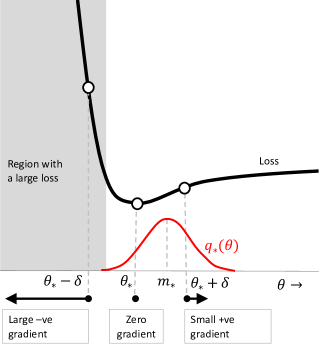
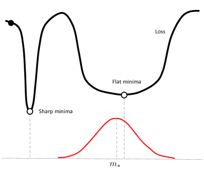
OGN’s uncertainty estimates can be improved further by relaxing the approximation made by the delta method and using Bayesian averaging through variational inference. This improves over Laplace’s method by using the stationarity conditions (Eqs. 25 and 26) where Bayesian averaging is employed through an expectation over $q(\text{$\boldsymbol{\theta}$})$ (Opper and Archambeau, 2009). The variational solution is slightly different than Laplace’s method and is expected to be more robust due to the averaging over $q_{*}(\text{$\boldsymbol{\theta}$})$ in Eqs. 25 and 26. Two such situations are illustrated in Fig. 1, one corresponding to an asymmetric loss where the Bayesian solution avoids a region with extremely high loss (Fig. 1), and the other one where it seeks a more stable solution involving a wide and shallow minimum compared to a sharp and deep minimum (Fig. 1). Such situations are hypothesised to exist in deep-learning problems (Hochreiter and Schmidhuber, 1997, 1995; Keskar et al., 2016), where a good performance of stochastic optimization methods is attributed to their ability to find shallow minima (Dziugaite and Roy, 2017). Similar strategies exist in stochastic search and global optimization literature where a kernel is used to convolve/smooth the objective function, like in Gaussian homotopy continuation method (Mobahi and Fisher III, 2015), optimization by smoothing (Leordeanu and Hebert, 2008), graduated optimization method (Hazan et al., 2016), and evolution strategies (Huning, 1976; Wierstra et al., 2014). The stochastic noise in these methods is akin to the Bayesian noise injected through the distribution $q(\text{$\boldsymbol{\theta}$})$. Unlike the ‘unregulated’ noise in these methods, the benefit of the Bayesian approach is that the noise source $q(\text{$\boldsymbol{\theta}$})$ can adapt itself from data by using the BLR.

Refer to caption
Refer to caption
Figure 1: Bayesian solutions have similar robustness properties to flatter minima found in deep learning via stochastic algorithms. Panel (a): When the minimum lies right next to a ‘wall’, the Bayesian solution shifts away from the wall (towards the flatter side) to avoid large losses under small perturbation. This is due to the averaging over $q_{*}(\text{$\boldsymbol{\theta}$})$ in condition Eq. 25. Panel (b): Given a sharp minimum vs a flat minimum, the Bayesian solution often prefers the flatter minimum, which is again due to the averaging over $q_{*}(\text{$\boldsymbol{\theta}$})$

.

The variational-Bayesian version is obtained by simply removing the approximation due to the delta method from Eq. 44, going back to the original Newton variant of Eq. 12 (now with minibatch Hessians),

$\displaystyle\text{$\boldsymbol{\theta}$}_{t+1}\leftarrow\text{$\boldsymbol{\theta}$}_{t}-\rho_{t}\frac{1}{\text{$\boldsymbol{s}$}_{t+1}}\circ\mathbb{E}_{q_{t}}\left[\widehat{\nabla}_{\text{\text{$\boldsymbol{\theta}$}}}\bar{\ell}(\text{$\boldsymbol{\theta}$})\right],\quad\text{with}\quad\text{$\boldsymbol{s}$}_{t+1}\leftarrow(1-\rho_{t})\text{$\boldsymbol{s}$}_{t}+\rho_{t}\,\,\mathbb{E}_{q_{t}}\left[\text{{diag}}(\widehat{\nabla}_{\text{\text{$\boldsymbol{\theta}$}}}^{2}\bar{\ell}(\text{$\boldsymbol{\theta}$}))\right],$ (46)

where iterates $q_{t}(\text{$\boldsymbol{\theta}$})=\text{${\cal N}$}(\text{$\boldsymbol{\theta}$}|\text{$\boldsymbol{\theta}$}_{t},\text{$\boldsymbol{S}$}_{t}^{-1})$ are defined with precision matrix $\text{$\boldsymbol{S}$}_{t}$ as a diagonal matrix with $\text{$\boldsymbol{s}$}_{t}$ as the diagonal. The iterates converge to an optimal diagonal Gaussian candidate that optimizes Eq. 2.

Similarly to OGN, the update Eq. 46 can be modified to use the Gauss-Newton approximation Eq. 45, which is easier to implement and can also exploit the deep-learning tricks to find good solutions. The expectations can be implemented by a simple ‘weight-perturbation’,

$$\mathbb{E}_{q_{t}}[\widehat{\nabla}_{\text{$\boldsymbol{\theta}$}}\bar{\ell}(\text{$\boldsymbol{\theta}$})]\approx\widehat{\nabla}_{\text{$\boldsymbol{\theta}$}}\bar{\ell}(\text{$\boldsymbol{\theta}$}_{t}+\text{$\boldsymbol{\epsilon}$}_{t})$$

where $\text{$\boldsymbol{\epsilon}$}_{t}\sim\text{${\cal N}$}(\text{$\boldsymbol{\epsilon}$}|0,\text{{diag}}(\text{$\boldsymbol{s}$}_{t}))$ (multiple samples can also be used). The resulting algorithm is referred to as variational OGN or VOGN by Khan et al. (2018)) and is shown to match the performance of Adam and give better uncertainty estimates than both Adam, OGN, and other Bayesian alternatives (Osawa et al., 2019, Fig. 1). A version with the FIM of the log-likelihood is proposed in Khan et al. (2019) (algorithm is called VOGGN). Variants that exploit Hessian structures using Kronecker-factored (Zhang et al., 2018b) and low-rank (Mishkin et al., 2018) are also considered in the literature.

4.5 Binary neural networks

Binary NNs have binary weights $\text{$\boldsymbol{\theta}$}\in\{-1,+1\}^{P}$, hence we need to consider another class of the candidate distributions than the Gaussian (we will choose Bernoulli). Binary NNs are natural candidates for resource-constrained applications, like mobile phones, wearable and IoT devices, but their training is challenging due to the binary weights for which gradients do not exists. Our Bayesian scheme solves this issue because gradients of the Bayesian objective are always defined with respect to the parameters of a Bernoulli distribution, turning a discrete problem into a continuous one. The discussion here is based on the results of Meng et al. (2020) who used the BLR to derive the BayesBiNN learning algorithm and connect it to the well known Straight-Through-Estimator (STE) (Bengio et al., 2013).

The training objective of binary NN involves a discrete optimization problem

$$\min_{\text{\text{$\boldsymbol{\theta}$}}\in\{-1,+1\}^{P}}\,\,\sum_{i=1}^{N}\ell(y_{i},f_{\text{\text{$\boldsymbol{\theta}$}}}(\text{$\boldsymbol{x}$}_{i})).$$ (47)

In theory, gradient based methods should not work for such problems since the gradients with respect to discrete variables do not exist. Still, the most popular method to train binary NN, the Straight-Through-Estimator (STE) (Bengio et al., 2013), employs continuous optimization methods and works remarkably well (Courbariaux et al., 2015). The method is justified based on latent real-valued weights $\tilde{\text{$\boldsymbol{\theta}$}}\in{}^{P}$ which are discretized at every iteration to get binary weights $\boldsymbol{\theta}$, while the gradients used to update the latent weights $\tilde{\text{$\boldsymbol{\theta}$}}$, are computed at the binary weights $\boldsymbol{\theta}$, as shown below,

$$\tilde{\text{$\boldsymbol{\theta}$}}_{t+1}\leftarrow\tilde{\text{$\boldsymbol{\theta}$}}_{t}-\alpha\sum_{i\in\mathcal{M}_{t}}\nabla_{\text{\text{$\boldsymbol{\theta}$}}}\ell(y_{i},f_{\text{\text{$\boldsymbol{\theta}$}}_{t}}(\text{$\boldsymbol{x}$}_{i})),\text{ where }\text{$\boldsymbol{\theta}$}_{t}\leftarrow\text{sign}(\tilde{\text{$\boldsymbol{\theta}$}}_{t})$$ (48)

It is not clear why the gradients computed at the binary weights help the search for the minimum of the discrete problem, and many studies have attempted to answer this question, e.g., see Yin et al. (2019); Alizadeh et al. (2019). The Bayesian objective in Eq. 2 rectify this issue since the expectation of a discrete objective is a continuous objective with respect to the parameters of the distributions, justifying the use of gradient based methods.

We will now show that using Bernoulli candidate distributions in the BLR gives rise to an algorithm similar to Eq. 48, justifying the application of the STE algorithm to solve a discrete optimization problem. Specifically, we choose $q(\theta_{j}=1)=p_{j}$ where $p_{j}\in[0,1]$ is the success probability. We also assume a mean-field distribution to get $q(\text{$\boldsymbol{\theta}$})=\prod_{j=1}^{P}q(\theta_{j})$. Since the Bernoulli distribution is a minimal exponential-family with a constant base measure, we use the BLR in Eq. 6 with $\lambda_{j}=1/2\log({p_{j}}/(1-p_{j}))$ and $\mu_{j}=2p_{j}-1$, to get

$\displaystyle\text{$\boldsymbol{\lambda}$}_{t+1}$ $\displaystyle\leftarrow(1-\rho_{t})\text{$\boldsymbol{\lambda}$}_{t}-\rho_{t}\nabla_{\text{$\boldsymbol{\mu}$}}\mathbb{E}_{q_{t}}\left[\sum_{i\in\mathcal{M}_{t}}\ell(y_{i},f_{\text{\text{$\boldsymbol{\theta}$}}}(\text{$\boldsymbol{x}$}_{i}))\right].$ (49)

The challenge now is to compute the gradient with respect to $\boldsymbol{\mu}$, but it turns out that approximating it with the Concrete distribution (Maddison et al., 2016; Jang et al., 2016) recovers the STE step.

Concrete distribution provides a way to relax a discrete random variable into a continuous one such that it becomes a deterministic function of a continuous random variable. Following Maddison et al. (2016), the continuous random variable, denoted by $\hat{\theta}^{(\tau)}\in(-1,1)$, are constructed from the binary variable $\theta\in\{-1,1\}$ by using iid uniform random variables $\epsilon\in(0,1)$ and using the function $\tanh(\cdot)$,

$$\hat{\theta}^{(\tau)}=\tanh\left(\frac{\lambda+\delta(\epsilon)}{\tau}\right),\text{ where }\delta(\epsilon)=\text{$\frac{1}{2}$}\log\left(\frac{\epsilon}{1-\epsilon}\right),$$ (50)

with $\tau>0$ as the temperature parameter. As $\tau\to 0$, the function approaches the sign function used in STE step (Eq. 48): $\hat{\theta}^{(0)}=\text{sign}(\lambda+\delta(\epsilon))$.

The gradient too can be approximated by the gradients with respect to the relaxed variables

$\displaystyle\nabla_{\text{\text{$\boldsymbol{\mu}$}}}\mathbb{E}_{q}\left[\ell(y_{i},f_{\text{\text{$\boldsymbol{\theta}$}}}(\text{$\boldsymbol{x}$}_{i}))\right]\approx\nabla_{\text{\text{$\boldsymbol{\mu}$}}}\ell(y_{i},f_{\hat{\text{\text{$\boldsymbol{\theta}$}}}^{(\tau)}}(\text{$\boldsymbol{x}$}_{i}))=\text{$\boldsymbol{s}$}\circ\left[\nabla_{\hat{\text{\text{$\boldsymbol{\theta}$}}}^{(\tau)}}\ell(y_{i},f_{\hat{\text{\text{$\boldsymbol{\theta}$}}}^{(\tau)}}(\text{$\boldsymbol{x}$}_{i}))\right],$ (51)

where we used chain rule in the last step and $\boldsymbol{s}$ is a vector of

$$s_{j}=\nabla_{\mu_{j}}\theta_{j}^{(\tau)}=\frac{1}{\tau}\left[\frac{1-(\hat{\theta}_{j}^{(\tau)})^{2}}{1-\tanh^{2}(\lambda_{j})}\right].$$

By renaming $\boldsymbol{\lambda}$ by $\tilde{\text{$\boldsymbol{\theta}$}}$ and $\hat{\text{$\boldsymbol{\theta}$}}^{(\tau)}$ by $\boldsymbol{\theta}$, the rule in Eq. 49 becomes

$\displaystyle\tilde{\text{$\boldsymbol{\theta}$}}_{t+1}\leftarrow(1-\rho_{t})\tilde{\text{$\boldsymbol{\theta}$}}_{t}-\rho_{t}\text{$\boldsymbol{s}$}_{t}\circ\left[\sum_{i\in\mathcal{M}_{t}}\nabla_{\text{\text{$\boldsymbol{\theta}$}}}\ell(y_{i},f_{\text{\text{$\boldsymbol{\theta}$}}_{t}}(\text{$\boldsymbol{x}$}_{i}))\right],\text{ where }$ $\displaystyle\text{$\boldsymbol{\theta}$}_{t}\leftarrow\tanh\left(\frac{1}{\tau}\left(\tilde{\text{$\boldsymbol{\theta}$}}_{t}+\text{$\boldsymbol{\delta}$}(\text{$\boldsymbol{\epsilon}$}_{t})\right)\right)$ (52)

with $\text{$\boldsymbol{s}$}_{t}\leftarrow(1-\text{$\boldsymbol{\theta}$}_{t}^{2})/(\tau(1-\tanh^{2}(\tilde{\text{$\boldsymbol{\theta}$}}_{t})))$, and $\text{$\boldsymbol{\epsilon}$}_{t}$ is a vector of $P$ iid samples from a uniform distribution. Meng et al. (2020) refer to this algorithm as BayesBiNN.

BayesBiNN is similar to STE shown in Eq. 48, but computes natural-gradients (instead of gradients) at the relaxed parameters $\text{$\boldsymbol{\theta}$}_{t}$ which are obtained by adding noise $\text{$\boldsymbol{\delta}$}(\text{$\boldsymbol{\epsilon}$}_{t})$ to the real-valued weights $\tilde{\text{$\boldsymbol{\theta}$}}_{t}$. The gradients are approximations of the expected loss and are well defined. By setting noise to zero and letting the temperature $\tau\to 0$, the $\tanh(\cdot/\tau)$ becomes the sign-function and we recover the gradients used in STE. This limit is when the randomness is ignored and is similar to the delta method used in earlier sections. The random noise $\text{$\boldsymbol{\delta}$}(\text{$\boldsymbol{\epsilon}$}_{t})$ and the non-zero temperature $\tau$ enables a softening of the binary weights, allowing for meaningful gradients. BayesBiNN also provides meaningful latent $\tilde{\text{$\boldsymbol{\theta}$}}$ which are now the natural parameters of the Bernoulli distribution.

Unlike STE, the updates employs a exponential smoothing which is a direct consequence of using the entropy term in the Bayesian objective. With discrete weights, optimum of Eq. 47 could be completely unrelated to an STE solution $\text{$\boldsymbol{\theta}$}_{*}$, for example, the one that yields zero gradients $\sum_{i}\nabla_{\text{\text{$\boldsymbol{\theta}$}}}\ell(y_{i},f_{\text{\text{$\boldsymbol{\theta}$}}_{*}}(\text{$\boldsymbol{x}$}_{i}))=0$. In contrast, the BayesBiNN solution minimizes the well-defined Bayes objective of Eq. 2, whose optimum is characterized by the optimality condition Eq. 24 directly relating the optimal $\tilde{\text{$\boldsymbol{\theta}$}}_{*}$ to the relaxed variables $\text{$\boldsymbol{\theta}$}_{*}$:

$\displaystyle\frac{\tilde{\text{$\boldsymbol{\theta}$}}_{*}}{\text{$\boldsymbol{s}$}_{*}}\approx\sum_{i=1}^{N}\nabla_{\text{\text{$\boldsymbol{\theta}$}}}\ell(y_{i},f_{\text{\text{$\boldsymbol{\theta}$}}_{*}}(\text{$\boldsymbol{x}$}_{i})).$ (53)

The BayesBiNN solution $\text{$\boldsymbol{\theta}$}_{*}$ is in general different from the one from the STE algorithm, but when temperature $\tau\to 0$ we expect the two solutions to be similar whenever $\text{$\boldsymbol{s}$}_{*}\to\infty$ (as the left-hand-side in the equation above goes to zero). In general, we expect the BayesBiNN solution to have robustness properties similar to the ones discussed for Fig. 1. The exponential smoothing used in BayesBiNN is similar to the update of Helwegen et al. (2019) but their formulation lacks a well-defined objective.

5 Probabilistic Inference Algorithms from the Bayesian Learning Rule

Algorithms for inference in probabilistic graphical models can be derived from the BLR, by setting the loss function to be the log-joint density of the data and unknowns. Unknowns could include both latent variables $\boldsymbol{z}$ and model parameters $\boldsymbol{\theta}$. The class ${\mathcal{Q}}$ is chosen based on the form of the likelihood and prior. We will first discuss the conjugate case, where BLR reduces to Bayes’ rule, and then discuss expectation maximization and variational inference (VI) where structural approximations to the posterior are employed.

5.1 Conjugate models and Bayes’ rule

We start with one of the most popular category of Bayesian models called exponential-family conjugate models. We consider $N$ i.i.d. data $\text{$\boldsymbol{y}$}_{i}$ with likelihoods $p(\text{$\boldsymbol{y}$}_{i}|\text{$\boldsymbol{\theta}$})$ (no latent variables) and prior $p(\text{$\boldsymbol{\theta}$})$. Conjugacy implies the existence of sufficient statistics $\text{$\boldsymbol{T}$}(\text{$\boldsymbol{\theta}$})$ such that both the likelihood and prior take an exponential form shown below

$$p(\text{$\boldsymbol{y}$}_{i}|\text{$\boldsymbol{\theta}$})\propto e^{\langle\widetilde{\text{$\boldsymbol{\lambda}$}}_{i}(\text{$\boldsymbol{y}$}_{i}),\text{$\boldsymbol{T}$}(\text{$\boldsymbol{\theta}$})\rangle},\quad\text{ and }\quad p(\text{$\boldsymbol{\theta}$})\propto e^{\langle\text{$\boldsymbol{\lambda}$}_{0},\text{$\boldsymbol{T}$}(\text{$\boldsymbol{\theta}$})\rangle},$$

for some $\widetilde{\text{$\boldsymbol{\lambda}$}}_{i}(\text{$\boldsymbol{y}$}_{i})$ (a function of $\text{$\boldsymbol{y}$}_{i}$), and $\text{$\boldsymbol{\lambda}$}_{0}$. For example, for ridge regression discussed in Sec. 1.3.3, the likelihoods and prior are

$\displaystyle p(y_{i}|\text{$\boldsymbol{\theta}$})$ $\displaystyle=\text{${\cal N}$}(y_{i}|\text{$\boldsymbol{x}$}_{i}^{\top}\text{$\boldsymbol{\theta}$},1)\propto e^{(y_{i}\text{$\boldsymbol{x}$}_{i})^{\top}\text{$\boldsymbol{\theta}$}+\text{Tr}\left(-\text{$\frac{1}{2}$}\text{$\boldsymbol{x}$}_{i}\text{$\boldsymbol{x}$}_{i}^{\top}\left(\text{$\boldsymbol{\theta}$}\text{$\boldsymbol{\theta}$}^{\top}\right)\right)-\text{$\frac{1}{2}$}y_{i}^{2}},$
$\displaystyle p(\text{$\boldsymbol{\theta}$})$ $\displaystyle=\text{${\cal N}$}(\text{$\boldsymbol{\theta}$}|0,\text{$\boldsymbol{I}$}/\delta)\propto e^{\text{Tr}\left(-\text{$\frac{1}{2}$}\delta\text{$\boldsymbol{I}$}\left(\text{$\boldsymbol{\theta}$}\text{$\boldsymbol{\theta}$}^{\top}\right)\right)},$

respectively, and, because $\text{$\boldsymbol{T}$}(\text{$\boldsymbol{\theta}$})=(\text{$\boldsymbol{\theta}$},\text{$\boldsymbol{\theta}$}\text{$\boldsymbol{\theta}$}^{\top})$, we have the following pairs

$$\begin{array}[]{ll}\begin{array}[]{ll}\widetilde{\text{$\boldsymbol{\lambda}$}}_{i}^{(1)}(y_{i})&=y_{i}\text{$\boldsymbol{x}$}_{i},\\ \widetilde{\text{$\boldsymbol{\lambda}$}}_{i}^{(2)}(y_{i})&=-\text{$\frac{1}{2}$}\text{$\boldsymbol{x}$}_{i}\text{$\boldsymbol{x}$}_{i}^{\top},\end{array}&\quad\begin{array}[]{ll}\text{$\boldsymbol{\lambda}$}_{0}^{(1)}&=0,\\ \text{$\boldsymbol{\lambda}$}_{0}^{(2)}&=-\text{$\frac{1}{2}$}\delta\text{$\boldsymbol{I}$}.\end{array}\end{array}$$

The quantity $\widetilde{\text{$\boldsymbol{\lambda}$}}_{i}(\text{$\boldsymbol{y}$}_{i})$ is often interpreted as the sufficient statistics of $\text{$\boldsymbol{y}$}_{i}$, but it can also be seen as the natural parameter of the likelihood with respect to $\text{$\boldsymbol{T}$}(\text{$\boldsymbol{\theta}$})$. The posterior is then obtained by a simple addition of these natural parameters, as shown below,

$$p(\text{$\boldsymbol{\theta}$}|\text{$\boldsymbol{y}$})\,\,\propto p(\text{$\boldsymbol{\theta}$})\prod_{i}p(\text{$\boldsymbol{y}$}_{i}|\text{$\boldsymbol{\theta}$})\,\,\propto\exp\left(\langle\text{$\boldsymbol{\lambda}$}_{0}+\sum_{i}\widetilde{\text{$\boldsymbol{\lambda}$}}_{i}(\text{$\boldsymbol{y}$}_{i}),\text{$\boldsymbol{T}$}(\text{$\boldsymbol{\theta}$})\rangle\right),$$

where $\text{$\boldsymbol{y}$}=(\text{$\boldsymbol{y}$}_{1},\text{$\boldsymbol{y}$}_{2},\ldots,\text{$\boldsymbol{y}$}_{N})$.

The natural-parameter of the posterior can be obtained from the BLR. To see this, we first note that the loss needed in the BLR is the negative of the log-joint density

$$\bar{\ell}(\text{$\boldsymbol{\theta}$})=-\log p(\text{$\boldsymbol{y}$},\text{$\boldsymbol{\theta}$})=-\log p(\text{$\boldsymbol{\theta}$})+\sum_{i=1}^{N}\left[-\log p(\text{$\boldsymbol{y}$}_{i}|\text{$\boldsymbol{\theta}$})\right].$$

The natural parameter of the posterior is recovered from the fixed point of the BLR (Eq. 5),

$$\begin{split}\text{$\boldsymbol{\lambda}$}_{*}=\nabla_{\text{\text{$\boldsymbol{\mu}$}}}\mathbb{E}_{q_{*}}[\log p(\text{$\boldsymbol{\theta}$})]+\sum_{i}\nabla_{\text{\text{$\boldsymbol{\mu}$}}}\mathbb{E}_{q_{*}}[\log p(\text{$\boldsymbol{y}$}_{i}|\text{$\boldsymbol{\theta}$})]=\text{$\boldsymbol{\lambda}$}_{0}+\sum_{i}\widetilde{\text{$\boldsymbol{\lambda}$}}_{i}(\text{$\boldsymbol{y}$}_{i}),\end{split}$$ (54)

which is equivalent to running the BLR for just one-iteration with $\rho_{t}=1$. For ridge regression, for instance, the above equation results in the natural gradients in Eq. 14 from which the ridge-regression solution can be recovered, as shown in Sec. 1.3.3.

In general, for such conjugate exponential-family models, the BLR yields the exact posterior by a direct application of Eq. 5. Applying Bayes’ rule there is equivalent to a single step of Eq. 6 with $\rho_{t}=1$. This includes popular Gaussian linear models (Roweis and Ghahramani, 1999), such as Kalman filter/smoother, probabilistic Principle Components Analysis (PCA), factor analysis, mixture of Gaussians, and hidden Markov models, as well as nonparameteric models, such as Gaussian process (GP) regression (Rasmussen and Williams, 2006). For all such cases, the BLR gives yields the natural parameter of the posterior in just one step. From a computational point of view, it does not offer any advice to obtain marginal properties in general, and, similarly to Bayes’ rule, efficient techniques, such as message passing, may be needed to perform the necessary computation.

5.2 Expectation maximization

We will now derive Expectation Maximization (EM) from the BLR with coordinate-wise updates with $\rho_{t}=1$, similarly to the conjugate case. In the subsequent sections, this connection is used to derive new stochastic VI algorithms where sometimes $\rho_{t}<1$ is used.

EM is a popular algorithm for parameter estimation with latent variables (Dempster et al., 1977). Given the joint distribution $p(\text{$\boldsymbol{y}$},\text{$\boldsymbol{z}$}|\text{$\boldsymbol{\theta}$})$ with latent variables $\boldsymbol{z}$ and parameters $\boldsymbol{\theta}$, the EM algorithm computes the posterior $p(\text{$\boldsymbol{z}$}|\text{$\boldsymbol{y}$},\text{$\boldsymbol{\theta}$}_{*})$ as well as parameter $\text{$\boldsymbol{\theta}$}_{*}$ that maximizes the marginal likelihood $p(\text{$\boldsymbol{y}$}|\text{$\boldsymbol{\theta}$})$. The algorithm can be seen as coordinate-wise BLR updates with $\rho_{t}=1$ to update candidate distribution that factorizes across $\boldsymbol{z}$ and $\boldsymbol{\theta}$,

$$q_{t}(\text{$\boldsymbol{z}$},\text{$\boldsymbol{\theta}$})=q_{t}(\text{$\boldsymbol{z}$})q_{t}(\text{$\boldsymbol{\theta}$})\,\,\propto\,\,e^{\langle\text{$\boldsymbol{\lambda}$}_{t},\text{$\boldsymbol{T}$}_{z}(\text{$\boldsymbol{z}$})\rangle}\text{${\cal N}$}(\text{$\boldsymbol{\theta}$}|\text{$\boldsymbol{\theta}$}_{t},\text{$\boldsymbol{I}$}),$$ (55)

where $\text{$\boldsymbol{\theta}$}_{t}$ denotes the mean of the Gaussian. The loss function is set to $\bar{\ell}(\text{$\boldsymbol{z}$},\text{$\boldsymbol{\theta}$})=-\log p(\text{$\boldsymbol{y}$},\text{$\boldsymbol{z}$}|\text{$\boldsymbol{\theta}$})$.

To ease the presentation, assume the likelihood, prior, and joint are expressed as

$\displaystyle p(\text{$\boldsymbol{y}$}|\text{$\boldsymbol{z}$},\text{$\boldsymbol{\theta}$})$ $\displaystyle\propto\exp\left(\langle\widetilde{\text{$\boldsymbol{\lambda}$}}_{1}(\text{$\boldsymbol{y}$},\text{$\boldsymbol{\theta}$}),\text{$\boldsymbol{T}$}_{z}(\text{$\boldsymbol{z}$})\rangle\right),$ $\displaystyle p(\text{$\boldsymbol{z}$}|\text{$\boldsymbol{\theta}$})\propto\exp\left(\langle\text{$\boldsymbol{\lambda}$}_{0}(\text{$\boldsymbol{\theta}$}),\text{$\boldsymbol{T}$}_{z}(\text{$\boldsymbol{z}$})\rangle\right),$
$\displaystyle p(\text{$\boldsymbol{y}$},\text{$\boldsymbol{z}$}|\text{$\boldsymbol{\theta}$})$ $\displaystyle\propto\exp\left(\langle\text{$\boldsymbol{T}$}_{yz}(\text{$\boldsymbol{y}$},\text{$\boldsymbol{z}$}),\text{$\boldsymbol{\theta}$}\rangle-A_{yz}(\text{$\boldsymbol{\theta}$})\right),$ (56)

for some functions $\widetilde{\text{$\boldsymbol{\lambda}$}}_{1}(\cdot,\cdot)$ and $\text{$\boldsymbol{\lambda}$}_{0}(\cdot)$ (similarly to the previous section), and $\boldsymbol{\theta}$ is the natural parameter of the joint. The likelihood and prior are expressed in terms of sufficient statistics $\text{$\boldsymbol{T}$}_{z}(\text{$\boldsymbol{z}$})$ while the joint is with $\text{$\boldsymbol{T}$}_{yz}(\cdot,\cdot)$ (Winn and Bishop, 2005). The EM algorithm then takes a simple form where we iterate between updating $\boldsymbol{\lambda}$ and $\boldsymbol{\theta}$ (Banerjee et al., 2005),

$$\text{E-step:}\quad\text{$\boldsymbol{\lambda}$}_{t+1}\leftarrow\widetilde{\text{$\boldsymbol{\lambda}$}}_{1}(\text{$\boldsymbol{y}$},\text{$\boldsymbol{\theta}$}_{t})+\text{$\boldsymbol{\lambda}$}_{0}(\text{$\boldsymbol{\theta}$}_{t}),\qquad\text{M-step:}\quad\text{$\boldsymbol{\theta}$}_{t+1}\leftarrow A^{*}_{yz}\left(\mathbb{E}_{q_{t+1}}[\text{$\boldsymbol{T}$}_{yz}(\text{$\boldsymbol{y}$},\text{$\boldsymbol{z}$})]\right).$$

Here, $A_{yz}^{*}(\cdot)$ is the Legendre transform, and $q_{t+1}(\text{$\boldsymbol{z}$})=p(\text{\text{$\boldsymbol{z}$}}|\text{$\boldsymbol{y}$},\text{$\boldsymbol{\theta}$}_{t+1})$ is the outcome of E-step.

The two steps are obtained from the BLR by using the delta method to approximate the expectation with respect to $q_{t}(\text{$\boldsymbol{\theta}$})$. For the E-step, we assume $q_{t}(\text{$\boldsymbol{\theta}$})$ fixed, and use Eqs. 5 and 54 and the delta method,

$$\text{$\boldsymbol{\lambda}$}_{t+1}\leftarrow\left.\nabla_{\text{$\boldsymbol{\mu}$}}\mathbb{E}_{q_{t}(\text{$\boldsymbol{z}$})q_{t}(\text{$\boldsymbol{\theta}$})}[-\bar{\ell}(\text{$\boldsymbol{z}$},\text{$\boldsymbol{\theta}$})]\right|_{\text{$\boldsymbol{\mu}$}=\text{$\boldsymbol{\mu}$}_{t}}=\mathbb{E}_{q_{t}(\text{$\boldsymbol{\theta}$})}[\widetilde{\text{$\boldsymbol{\lambda}$}}_{1}(\text{$\boldsymbol{y}$},\text{$\boldsymbol{\theta}$})+\text{$\boldsymbol{\lambda}$}_{0}(\text{$\boldsymbol{\theta}$})]\approx\widetilde{\text{$\boldsymbol{\lambda}$}}_{1}(\text{$\boldsymbol{y}$},\text{$\boldsymbol{\theta}$}_{t})+\text{$\boldsymbol{\lambda}$}_{0}(\text{$\boldsymbol{\theta}$}_{t})$$

For the M-step, we use the stationarity condition similar to Eq. 25 but now with the delta method with respect to $q(\text{$\boldsymbol{\theta}$})$ (note that $\text{$\boldsymbol{\theta}$}_{t+1}$ is both the expectation and natural parameter),

$$\left.\nabla_{\text{$\boldsymbol{\theta}$}}\mathbb{E}_{q_{t+1}(\text{$\boldsymbol{z}$})}\left[\bar{\ell}(\text{$\boldsymbol{z}$},\text{$\boldsymbol{\theta}$})\right]\right|_{\text{$\boldsymbol{\theta}$}=\text{$\boldsymbol{\theta}$}_{t+1}}=0$$

A simple calculation using the joint $p(\text{$\boldsymbol{y}$},\text{$\boldsymbol{z}$})$ will show that this reduces to the M-step.

The derivation is easily extended to the generalized EM iterations. The coordinate-wise strategy also need not be employed and the BLR steps can also be run in parallel. Such scheme resembles the generalized EM algorithm and usually converges faster. Online schemes can be obtained by using stochastic gradients, similar to those considered in Titterington (1984); Neal and Hinton (1998); Sato (1999); Cappé and Moulines (2009); Delyon et al. (1999). More recently, Amid and Warmuth (2020) use a divergence-based approach and Kunstner et al. (2021) prove attractive convergence properties using a mirror-descent formulation similar to ours. Next, we derive a generalization of such online schemes, called the stochastic variational inference.

5.3 Stochastic variational inference and variational message passing

Stochastic variational inference (SVI) is a generalization of EM, first considered by Sato (2001) for the conjugate case and extended by Hoffman et al. (2013) to conditionally-conjugate models (a similar strategy was also proposed by Honkela et al. (2011)). We consider the conjugate case due to its simplicity. The model is assumed to be similar to the EM case as in Eq. 56, but with $N$ iid data examples $\text{$\boldsymbol{y}$}_{i}$ associated with one latent vector $\text{$\boldsymbol{z}$}_{i}$ each and a conjugate prior $p(\text{$\boldsymbol{\theta}$}|\text{$\boldsymbol{\alpha}$})$ with $\text{$\boldsymbol{\alpha}$}=(\text{$\boldsymbol{\alpha}$}_{1},\alpha_{2})$ as prior parameters,

$\displaystyle p(\text{$\boldsymbol{y}$}_{i}|\text{$\boldsymbol{z}$}_{i},\text{$\boldsymbol{\theta}$})$ $\displaystyle\propto\exp\left(\langle\widetilde{\text{$\boldsymbol{\lambda}$}}_{i}(\text{$\boldsymbol{y}$}_{i},\text{$\boldsymbol{\theta}$}),\text{$\boldsymbol{T}$}_{i}(\text{$\boldsymbol{z}$}_{i})\rangle\right),$ $\displaystyle p(\text{$\boldsymbol{z}$}_{i}|\text{$\boldsymbol{\theta}$})\propto\exp\left(\langle\text{$\boldsymbol{\lambda}$}_{0}(\text{$\boldsymbol{\theta}$}),\text{$\boldsymbol{T}$}_{i}(\text{$\boldsymbol{z}$}_{i})\rangle\right),$
$\displaystyle p(\text{$\boldsymbol{y}$}_{i},\text{$\boldsymbol{z}$}_{i}|\text{$\boldsymbol{\theta}$})$ $\displaystyle\propto\exp\left(\langle\text{$\boldsymbol{T}$}_{yz}(\text{$\boldsymbol{y}$}_{i},\text{$\boldsymbol{z}$}_{i}),\text{$\boldsymbol{\theta}$}\rangle-A_{yz}(\text{$\boldsymbol{\theta}$})\right),$ $\displaystyle p(\text{$\boldsymbol{\theta}$}|\text{$\boldsymbol{\alpha}$})=h_{0}(\text{$\boldsymbol{\theta}$})\exp\left(\left[\langle\text{$\boldsymbol{\alpha}$}_{1},\text{$\boldsymbol{\theta}$}\rangle-\alpha_{2}A_{yz}(\text{$\boldsymbol{\theta}$})\right]\right).$ (57)

Due to conjugacy, each conditional update can be done coordinate wise. A common strategy is to assume a mean-field approximation

$$q(\text{$\boldsymbol{z}$}_{1},\ldots,\text{$\boldsymbol{z}$}_{N},\text{$\boldsymbol{\theta}$})=q(\text{$\boldsymbol{\theta}$})\prod_{i}q(\text{$\boldsymbol{z}$}_{i})\,\,\propto\,\,e^{\text{$\boldsymbol{\lambda}$}_{0}^{(1)}-\lambda_{0}^{(2)}A_{yz}(\text{$\boldsymbol{\theta}$})}\prod_{i}e^{\langle\text{$\boldsymbol{\lambda}$}_{i},\text{$\boldsymbol{T}$}_{i}(\text{$\boldsymbol{z}$}_{i})\rangle},$$

where $\text{$\boldsymbol{\lambda}$}_{i}$ is the natural parameter of $q(\text{$\boldsymbol{z}$}_{i})$, and $(\text{$\boldsymbol{\lambda}$}_{0}^{(1)},\lambda_{0}^{(2)})$ is the same for $q(\text{$\boldsymbol{\theta}$})$.

Coordinate-wise updates when applied to general graphical model are known as variational message passing (Winn and Bishop, 2005). These updates are a special case of BLR, applied coordinate wise with $\rho_{t}=1$. The derivation is almost identical to the one used for the EM case earlier, therefore omitted. One important difference is that, we do not employ the delta method for $q(\text{$\boldsymbol{\theta}$})$ and explicitly carry out the marginalization which has a closed-form expression due to conjugacy. The update for $q(\text{$\boldsymbol{\theta}$})$ is therefore replaced by its corresponding conjugate update.

Stochastic variational inference employs a special update where, after every $q(\text{$\boldsymbol{z}$}_{i})$ update with $\rho_{t}=1$, we update $q(\text{$\boldsymbol{\theta}$})$ but with $\rho_{t}<1$. Clearly, this is also covered as a special case of the BLR. The BLR update is more general than these strategies since it applies to a wider class of non-conjugate models, as discussed next.

5.4 Non-conjugate variational inference

Consider a graphical model $p(\text{$\boldsymbol{x}$})\propto\prod_{i\in{\mathcal{I}}}f_{i}(\text{$\boldsymbol{x}$}_{i})$ where $\boldsymbol{x}$ denotes the set of latent variables $\boldsymbol{z}$ and parameters $\boldsymbol{\theta}$ and $f_{i}(\text{$\boldsymbol{x}$}_{i})$ is the $i$’th factor operating on the subset $\text{$\boldsymbol{x}$}_{i}$ indexed by the set ${\mathcal{I}}$. The BLR can be applied to estimate a minimal exponential-family (assuming a constant base measure),

$$\text{$\boldsymbol{\lambda}$}_{t+1}\leftarrow(1-\rho_{t})\text{$\boldsymbol{\lambda}$}_{t}+\rho_{t}\sum_{i\in{\mathcal{I}}}\widetilde{\text{$\boldsymbol{\lambda}$}}_{i}(\text{$\boldsymbol{\mu}$}_{t}),\text{ where }\widetilde{\text{$\boldsymbol{\lambda}$}}_{i}(\text{$\boldsymbol{\mu}$}_{t})=\left.\nabla_{\boldsymbol{\mu}}\mathbb{E}_{q}\left[\log f_{i}(\text{$\boldsymbol{x}$}_{i})\right]\right|_{\text{$\boldsymbol{\mu}$}=\text{$\boldsymbol{\mu}$}_{t}},$$ (58)

and $\text{$\boldsymbol{\mu}$}_{t}=\nabla_{\text{$\boldsymbol{\lambda}$}}A(\text{$\boldsymbol{\lambda}$}_{t})$. We already encountered the quantities $\widetilde{\text{$\boldsymbol{\lambda}$}}_{i}(\text{$\boldsymbol{\mu}$}_{t})$ for conjugate models in Sec. 5.1 where they are referred to as the natural parameter of the factors. They can also be interpreted as “local” messages that are aggregated to obtain the “global” natural parameter $\text{$\boldsymbol{\lambda}$}_{t+1}$.

The update is quite flexible and can also be applied to other graphical models, such as Bayesian networks, Markov random fields, and Boltzmann machines. We can also view it as an update over distributions, by multiplying by $\text{$\boldsymbol{T}$}(\text{$\boldsymbol{x}$})$ followed by exponentiation,

$$q_{t+1}(\text{$\boldsymbol{x}$})\propto q_{t}(\text{$\boldsymbol{x}$})^{(1-\rho_{t})}\left[\prod_{i\in{\mathcal{I}}}\exp{\left(\langle\widetilde{\text{$\boldsymbol{\lambda}$}}_{i}(\text{$\boldsymbol{\mu}$}_{t}),\text{$\boldsymbol{T}$}(\text{$\boldsymbol{x}$})\rangle\right)}\right]^{\rho_{t}}$$ (59)

and at convergence

$$q_{*}(\text{$\boldsymbol{x}$})\propto\prod_{i\in{\mathcal{I}}}\exp{\left(\langle\widetilde{\text{$\boldsymbol{\lambda}$}}_{i}(\text{$\boldsymbol{\mu}$}_{*}),\text{$\boldsymbol{T}$}(\text{$\boldsymbol{x}$})\rangle\right)},$$

where $q_{*}(\text{$\boldsymbol{x}$})$ is the optimal distribution with natural and expectation parameters as $\text{$\boldsymbol{\lambda}$}_{*}$ and $\text{$\boldsymbol{\mu}$}_{*}$. This update has three important features.

  1. 1.

    The optimal $q_{*}(\text{$\boldsymbol{x}$})$ has the same structure as $p(\text{$\boldsymbol{x}$})$ and each term in $q_{*}(\text{$\boldsymbol{x}$})$ yields an approximation to those in $p(\text{$\boldsymbol{x}$})$,

    $$\log f_{i}(\text{$\boldsymbol{x}$}_{i})\approx\langle\widetilde{\text{$\boldsymbol{\lambda}$}}_{i}(\text{$\boldsymbol{\mu}$}_{*}),\text{$\boldsymbol{T}$}(\text{$\boldsymbol{x}$})\rangle+c_{i}$$

    for some constant $c_{i}$. The quantity $\widetilde{\text{$\boldsymbol{\lambda}$}}_{i}(\cdot)$ can be interpreted as the natural parameter of the local approximation. Such local parameters are often referred to as the site parameters in expectation propagation (EP) where their computations are often rather involved. In our formulation they are simply the natural gradients of the expected log joint density. See Chang et al. (2020, Sec. 3.4 and 3.5) for an example comparing the two. The above local approximations are inherently superior to the local-variational bounds, for example, quadratic bounds used in logistic regression (Jaakkola and Jordan, 1996; Khan et al., 2010, 2012; Khan, 2012), and also to the augmentation strategies (Girolami and Rogers, 2006; Klami, 2015). Gaussian posteriors give rise to quadratic surrogates to the loss function. These can be seen as alternatives to those obtained using Taylor’s expansion. The advantage of our surrogates is that they are not tight locally, rather globally Opper and Archambeau (2009).

  2. 2.

    The update in Eq. 59 yields both the local $\widetilde{\text{$\boldsymbol{\lambda}$}}_{i}(\cdot)$ and global $\boldsymbol{\lambda}$ parameters simultaneously, which is unlike the message-passing strategies that only compute the local messages. In fact, Eq. 59 can also be reformulated entirely in terms of local parameters (denoted by $\widetilde{\text{$\boldsymbol{\lambda}$}}_{i}^{(t+1)}$ below),

    $$\text{$\boldsymbol{\lambda}$}_{t+1}\leftarrow\sum_{i\in{\mathcal{I}}}\widetilde{\text{$\boldsymbol{\lambda}$}}_{i}^{(t+1)},\text{ where }\widetilde{\text{$\boldsymbol{\lambda}$}}_{i}^{(t+1)}\leftarrow(1-\rho_{t})\widetilde{\text{$\boldsymbol{\lambda}$}}_{i}^{(t)}+\rho_{t}\widetilde{\text{$\boldsymbol{\lambda}$}}_{i}(\text{$\boldsymbol{\mu}$}_{t}),$$ (60)

    This formulation was discussed by Khan and Lin (2017) who show this to be a generalization of the non-conjugate variational message passing algorithm (Knowles and Minka, 2011). The form is suitable for a distributed implementation using a message-passing framework.

  3. 3.

    The update applies to both conjugate and non-conjugate factors, but also for both probabilistic and deterministic variables. Automatic differentiation tools can be easily integrated. Due to such properties, the BLR offers an attractive framework for practical probabilistic programming (van de Meent et al., 2018).

We have argued that natural gradients play an important role for probabilistic inference, both for conjugate models or within those using message-passing frameworks. Still, their importance is somehow missed in the community. Natural gradients were first introduced in this context by Khan and Lin (2017); Khan et al. (2018), although Salimans and Knowles (2013) also mention a similar condition without an explicit reference to natural gradients. Sheth and Khardon (2016); Sheth (2019) discuss an update similar to the BLR for a specific case of two-level graphical models. Salimbeni et al. (2018) propose natural-gradient strategies for sparse GPs by using automatic differentiation which is often slower (the original work by Hensman et al. (2013), is also a special case of the BLR). A recent generalization to structured natural-gradient by Lin et al. (2021) is also worth noting.

We will end the section by discussing the connections of the BLR to the algorithms used in online learning, where the loss functions are observed sequentially at every iteration $t$,

$$q_{t+1}(\text{$\boldsymbol{\theta}$})=\operatorname*{arg\,min}_{q(\text{\text{$\boldsymbol{\theta}$}})}\quad\mathbb{E}_{q}\left[\ell(y_{t},f_{\text{\text{$\boldsymbol{\theta}$}}}(\text{$\boldsymbol{x}$}_{t}))\right]+\frac{1}{\rho_{t}}\mathbb{D}_{KL}[q(\text{$\boldsymbol{\theta}$})\,\|\,q_{t}(\text{$\boldsymbol{\theta}$})].$$

The resulting updates are called Exponential-Weight (EW) updates (Littlestone and Warmuth, 1994; Vovk, 1990), which are closely related to Bayes’ rule. van der Hoeven et al. (2018) show that, by approximating the first term by a surrogate (linear/quadratic) at the posterior mean (the delta method), many existing online learning algorithms can be obtained as special cases. This includes, online gradient descent, online Newton step, online mirror descent, among many others. This derivation is similar to the BLR which, when applied here, is slightly more general, not only due to the use of expectated loss, but also because the surrogate choice is automatically obtained by the posterior approximations.

An advantage of this connection is that the theoretical guarantees derived in online learning can be translated to the BLR, and consequently to all the learning-algorithms derived from it. We will also note that the local and global BLR updates presented in Eqs. 58 and 60 are similar to the ‘greedy’ and ‘lazy’ updates used in online learning (van der Hoeven et al., 2018). The conjugate case discussed in earlier sections are very similar to the algorithms proposed for online learning by Azoury and Warmuth (2001), which are concurrent to a similar proposal in the Bayesian community by Sato (2001).

6 Discussion

To learn, we need to extract useful information from new data and revise our beliefs. To do this well, we must reject false information and, at the same time, not ignore any (real) information. A good learning algorithm too must possess these properties. We expect the same to be true for the algorithms that have “stood the test of time” in terms of good performance, even if they are derived through empirical experimentation and intuitions. If there exist an optimal learning-algorithm, as it is often hypothesized, then we might be able to view these empirically good learning-algorithms as derived from this common origin. They might not be perfect but we might expect them to be a reasonable approximation of the optimal learning-algorithm. All in all, it is possible that all such algorithms optimize similar objectives and use similar strategies on how the optimization proceeds.

In this paper we argue for two ideas. The first is that the learning-objective is a Bayesian one and uses the variational formulation by Zellner (1988) in Eq. 2. The objective tells us how to balance new information with the old one, resulting ultimately in Bayes theorem as the optimal information processing rule. The power of the variational formulation, is that it also shows how to process the information when we have limited abilities, for example, in terms of computation, to extract the relevant information. The role of $q(\text{$\boldsymbol{\theta}$})$ is to define how to represent the knowledge, for which exponential families and mixtures thereof, are natural choices that have shown to balance complexity while still being practical.

The second idea is the role natural gradients play in the learning algorithms. Bayes’ rule in its original form has no opinion about them, but they are inherently present in all solutions of the Bayesian objective. They give us information about the learning-loss landscape, sometimes in the form of the derivatives of the loss and sometimes as the messages in a graphical model. Our work shows that all these seemingly different ideas, in fact, have deep roots in information geometry that is being exploited by natural gradients and then in Bayesian Learning Rule (BLR) we proposed.

The two ideas go together as a symbiosis into the BLR. By a long series of examples from optimisation, deep learning, and graphical models, we demonstrate that classical algorithms such as ridge regression, Newton’s method, and Kalman filter, as well as modern deep-learning algorithms such as stochastic-gradient descent, RMSprop, and Dropout, all can be derived from the proposed BLR. The BLR gives a unified framework and understanding of what various (good) learning algorithms do, how they differ in approximating the target and then also how they can be improved. The main advantage of the BLR, is that we now have a principled framework to approach new learning problems, both in terms of what to aim for and also how to get there.

Acknowledgement

M. E. Khan would like to thank many current and past colleagues at RIKEN-AIP, including W. Lin, D. Nielsen, X. Meng, T. Möllenhoff and P. Alquier, for many insightful discussions that helped shape parts of this paper. We also thank the anonymous reviewers for their feedback to improve the presentation.

Appendix A Bayesian inference as optimization

Bayesian inference is a special case of the Bayesian learning problem. Although this follows directly from the variational formulation by Zellner (1988), it might be useful to provide some more motivation. Bayesian inference corresponds to a log-likelihood loss $\ell(y,f_{\mathbf{\theta}}(\text{$\boldsymbol{x}$}))=-\log p(y|f_{\mathbf{\theta}}(\text{$\boldsymbol{x}$}))$. With conditional independent data and prior $p(\text{$\boldsymbol{\theta}$})$, the posterior distribution is $p(\text{$\boldsymbol{\theta}$}|\text{${\cal D}$})=p(\text{$\boldsymbol{\theta}$})/\mathcal{Z}(\text{${\cal D}$})\prod_{i=1}^{N}p(\text{$\boldsymbol{y}$}_{i}|f_{\theta}(\text{$\boldsymbol{x}$}_{i}))$. The minimizer of the Bayesian learning problem recovers this posterior distribution. This follows directly from reorganizing the Bayesian objective Eq. 2:

$\displaystyle\mathcal{L}(q)$ $\displaystyle=-\mathbb{E}_{q(\mathbf{\theta})}\left[\sum_{i=1}^{N}\log p(y_{i}|f_{\mathbf{\theta}}(\text{$\boldsymbol{x}$}_{i}))\right]+\mathbb{D}_{KL}[q(\text{$\boldsymbol{\theta}$})\,\|\,p(\text{$\boldsymbol{\theta}$})]$ (61)
$\displaystyle=\mathbb{E}_{q(\mathbf{\theta})}\left[\log\frac{q(\text{$\boldsymbol{\theta}$})}{\frac{p(\text{$\boldsymbol{\theta}$})}{\mathcal{Z}(\mathcal{D})}\prod_{i=1}^{N}p(y_{i}|f_{\mathbf{\theta}}(\text{$\boldsymbol{x}$}_{i}))}\right]+\log\mathcal{Z}(\text{${\cal D}$})$ (62)
$\displaystyle=\mathbb{D}_{KL}[q(\text{$\boldsymbol{\theta}$})\,\|\,p(\text{$\boldsymbol{\theta}$}|\text{${\cal D}$})]+\log\mathcal{Z}(\text{${\cal D}$})$ (63)

Choosing $q(\text{$\boldsymbol{\theta}$})$ as $p(\text{$\boldsymbol{\theta}$}|\text{${\cal D}$})$ minimizes the above equation since $\mathcal{Z}(\text{${\cal D}$})$ is a constant, and the KL divergence is zero.

Appendix B Natural gradient of the entropy

Here, we show that $\widetilde{\nabla}_{\text{$\boldsymbol{\lambda}$}}\mathcal{H}(q)=-\text{$\boldsymbol{\lambda}$}$ when $h(\text{$\boldsymbol{\theta}$})$ is a constant. First, we write

$$\begin{split}-\widetilde{\nabla}_{\text{$\boldsymbol{\lambda}$}}\mathcal{H}(q)&=\nabla_{\text{$\boldsymbol{\mu}$}}\mathbb{E}_{q}[\log q(\text{$\boldsymbol{\theta}$})]\\ &=\nabla_{\text{$\boldsymbol{\mu}$}}\left[\langle\text{$\boldsymbol{\lambda}$},\text{$\boldsymbol{\mu}$}\rangle-A(\text{$\boldsymbol{\lambda}$})\right]+\nabla_{\text{$\boldsymbol{\mu}$}}\mathbb{E}_{q}[\log h(\text{$\boldsymbol{\theta}$})]\\ &=\text{$\boldsymbol{\lambda}$}+\left(\nabla_{\text{$\boldsymbol{\lambda}$}}^{2}A(\text{$\boldsymbol{\lambda}$})\right)^{-1}\left[\text{$\boldsymbol{\mu}$}-\nabla_{\text{$\boldsymbol{\lambda}$}}A(\text{$\boldsymbol{\lambda}$})\right]+\nabla_{\text{$\boldsymbol{\mu}$}}\mathbb{E}_{q}[\log h(\text{$\boldsymbol{\theta}$})]\\ &=\text{$\boldsymbol{\lambda}$}+\nabla_{\text{$\boldsymbol{\mu}$}}\mathbb{E}_{q}[\log h(\text{$\boldsymbol{\theta}$})],\end{split}$$ (64)

where in the second line we use the definition of $q(\text{$\boldsymbol{\theta}$})$ and in the third line we use chain-rule and the fact that $\text{$\boldsymbol{\mu}$}=\nabla_{\text{$\boldsymbol{\lambda}$}}A(\text{$\boldsymbol{\lambda}$})$. For constant $h(\text{$\boldsymbol{\theta}$})$, this reduces to $\boldsymbol{\lambda}$, giving us the result.

Appendix C The delta method

In the delta method (Dorfman, 1938; Ver Hoef, 2012), we approximate the expectation of a function of a random variable by the expectation of the function’s Taylor expansion. For example, given a distribution $q(\text{$\boldsymbol{\theta}$})$ with mean $\boldsymbol{m}$, we can use the first-order Taylor approximation to get,

$$\mathbb{E}_{q}[f(\text{$\boldsymbol{\theta}$})]\approx\mathbb{E}_{q}\left[f(\text{$\boldsymbol{m}$})+(\text{$\boldsymbol{\theta}$}-\text{$\boldsymbol{m}$})^{\top}\left.\nabla_{\text{$\boldsymbol{\theta}$}}f(\text{$\boldsymbol{\theta}$})\right|_{\text{$\boldsymbol{\theta}$}=\text{$\boldsymbol{m}$}}\right]\,\,\approx f(\text{$\boldsymbol{m}$})$$

We will often use this approximation to approximate the expectation of gradient/Hessian at their values at a single point (usually the mean). For example, we can use a zeroth-order expansion to get

$$\mathbb{E}_{q}[\nabla_{\text{$\boldsymbol{\theta}$}}f(\text{$\boldsymbol{\theta}$})]\approx\left.\nabla_{\text{$\boldsymbol{\theta}$}}f(\text{$\boldsymbol{\theta}$})\right|_{\text{$\boldsymbol{\theta}$}=\text{$\boldsymbol{m}$}}\qquad\mathbb{E}_{q}[\nabla^{2}_{\text{$\boldsymbol{\theta}$}}f(\text{$\boldsymbol{\theta}$})]\approx\left.\nabla_{\text{$\boldsymbol{\theta}$}}^{2}f(\text{$\boldsymbol{\theta}$})\right|_{\text{$\boldsymbol{\theta}$}=\text{$\boldsymbol{m}$}}.$$

A better derivation (to get the same result) would be use higher-order expansion. For example, by using the first-order Taylor expansion, we approximate below the expectation of the gradient by the gradient at the mean,

$\displaystyle\mathbb{E}_{q}[\nabla_{\text{$\boldsymbol{\theta}$}}f(\text{$\boldsymbol{\theta}$})]$ $\displaystyle=\nabla_{\text{$\boldsymbol{m}$}}\mathbb{E}_{q}[f(\text{$\boldsymbol{\theta}$})]$
$\displaystyle\approx\nabla_{\text{$\boldsymbol{m}$}}\mathbb{E}_{q}\left[f(\text{$\boldsymbol{m}$})+(\text{$\boldsymbol{\theta}$}-\text{$\boldsymbol{m}$})^{\top}\left.\nabla_{\text{$\boldsymbol{\theta}$}}f(\text{$\boldsymbol{\theta}$})\right|_{\text{$\boldsymbol{\theta}$}=\text{$\boldsymbol{m}$}}\right]$
$\displaystyle=\left.\nabla_{\text{$\boldsymbol{\theta}$}}f(\text{$\boldsymbol{\theta}$})\right|_{\text{$\boldsymbol{\theta}$}=\text{$\boldsymbol{m}$}},$ (65)

where the first line is due to Bonnet’s theorem (App. D) and the second line is simply the first-order Taylor expansion. We refer to this as the first-order delta method. Similar applications have been used in variational inference (Blei and Lafferty, 2007; Braun and McAuliffe, 2010; Wang and Blei, 2013).

Similarly, by using the second-order Taylor expansion, we approximate below the expectation of the Hessian by the Hessian at the mean,

$\displaystyle\mathbb{E}_{q}[\nabla_{\text{$\boldsymbol{\theta}$}}^{2}f(\text{$\boldsymbol{\theta}$})]$ $\displaystyle=2\nabla_{\text{$\boldsymbol{S}$}^{-1}}\mathbb{E}_{q}[f(\text{$\boldsymbol{\theta}$})]$
$\displaystyle\approx 2\nabla_{\text{$\boldsymbol{S}$}^{-1}}\mathbb{E}_{q}\left[f(\text{$\boldsymbol{m}$})+(\text{$\boldsymbol{m}$}-\text{$\boldsymbol{\theta}$})^{\top}\left.\nabla_{\text{$\boldsymbol{\theta}$}}f(\text{$\boldsymbol{\theta}$})\right|_{\text{$\boldsymbol{\theta}$}=\text{$\boldsymbol{m}$}}+\text{$\frac{1}{2}$}(\text{$\boldsymbol{m}$}-\text{$\boldsymbol{\theta}$})^{\top}\left.\nabla_{\text{$\boldsymbol{\theta}$}}^{2}f(\text{$\boldsymbol{\theta}$})\right|_{\text{$\boldsymbol{\theta}$}=\text{$\boldsymbol{m}$}}(\text{$\boldsymbol{m}$}-\text{$\boldsymbol{\theta}$})\right]$
$\displaystyle=2\nabla_{\text{$\boldsymbol{S}$}^{-1}}\text{Tr}\left[\text{$\frac{1}{2}$}\text{$\boldsymbol{S}$}^{-1}\left.\nabla_{\text{$\boldsymbol{\theta}$}}^{2}f(\text{$\boldsymbol{\theta}$})\right|_{\text{$\boldsymbol{\theta}$}=\text{$\boldsymbol{m}$}}\right]$
$\displaystyle=\left.\nabla_{\text{$\boldsymbol{\theta}$}}^{2}f(\text{$\boldsymbol{\theta}$})\right|_{\text{$\boldsymbol{\theta}$}=\text{$\boldsymbol{m}$}},$ (66)

where the first line is due to Price’s theorem (App. D) and the second line is simply the second-order Taylor expansion. We refer to this as the second-order delta method.

C.1 Deterministic Estimates as crude-Bayesians

In ML it is often argued that deterministic estimates/models can be seen as a special case of probabilistic ones where variables are set to their maximum-a-posterior (MAP) estimates. One justification stems from the fact that such estimates can be seen as a posterior which is a Dirac-delta distribution at the MAP estimate; see Buntine (2002); Girolami and Kabán (2003); Gal (2016) for examples. The argument is then to use the delta distribution as a solution to the Bayesian objective (the evidence lower bound), justifying the MAP estimate as a Bayesian solution.

Formally, denoting the MAP estimate as $\text{$\boldsymbol{\theta}$}_{*}$, we can define a distribution $q_{\sigma}(\text{$\boldsymbol{\theta}$})=\text{${\cal N}$}(\text{$\boldsymbol{\theta}$}|\text{$\boldsymbol{\theta}$}_{*},\sigma\text{$\boldsymbol{I}$})$ By taking $\sigma\to 0$, we can view $\mathcal{L}(q_{\sigma})$ as the Bayesian solution obtained by a non-Bayesian MAP estimate. Unfortunately, this argument is flawed when estimating continuous parameters of deterministic models, as shown by Welling et al. (2008). This is because, as $\sigma\to 0$, the entropy $\mathcal{H}(q)=P\log\sigma\to-\infty$, making the objective useless. Therefore, it is not correct to use delta distributions to justify deterministic solutions as probabilistic and Bayesian ones.

Instead, we use the Delta method and obtain MAP estimates as a crude Bayesian approximation of the expectation. In this method, we do not set the posterior as a Dirac delta, rather we use a posterior approximation with a pre-specified uncertainty. For example, we can use a Gaussian

$$q_{*}(\text{$\boldsymbol{\theta}$})=\text{${\cal N}$}(\text{$\boldsymbol{\theta}$}|\text{$\boldsymbol{\theta}$}_{*},\text{$\boldsymbol{H}$}_{*}^{-1})$$

where $\text{$\boldsymbol{H}$}_{*}$ is the Hessian of ${\bar{\ell}}(\text{$\boldsymbol{\theta}$})$ or a positive-definite approximation of it when $\text{$\boldsymbol{H}$}_{*}$ itself is not. This is the Laplace’s method where the curvature around $\text{$\boldsymbol{\theta}$}_{*}$ is used as an uncertainty estimate. The choice views the MAP estimate as a crude-Bayesian because, by using the Delta method, we can replace the expectation by loss at the mean $\text{$\boldsymbol{\theta}$}_{*}$,

$$\mathbb{E}_{q}[\bar{\ell}(\text{$\boldsymbol{\theta}$})]-\mathcal{H}(q)\,\,\approx\,\,\bar{\ell}(\text{$\boldsymbol{\theta}$}_{*})+\text{$\frac{1}{2}$}P\log|\text{$\boldsymbol{H}$}_{*}|$$

which is exactly the objective optimized by $\text{$\boldsymbol{\theta}$}_{*}$ (the second term being a constant). A crude-Bayesian ignores the uncertainty around the estimate and simply uses the mean to approximate the expectation.

A similar view was presented in Opper and Archambeau (2009) where Laplace’s method was shown to be a crude-approximation of the variational method. However, in our argument the posterior covariance can be an arbitrary quantity, and even the posterior form does not need to be a Gaussian. The Delta method view is more general than the Laplace’s view of Opper and Archambeau (2009).

Appendix D Newton’s method from the BLR

We start by expressing the natural gradients in terms of the gradient with respect to the mean and covariance. Let $\boldsymbol{\theta}$ be multivariate normal with mean $\boldsymbol{\mu}$ and covariance $\boldsymbol{C}$, and $h(\text{$\boldsymbol{\mu}$},\text{$\boldsymbol{C}$})$ be a differentiable function. First, we write $\boldsymbol{m}$ and $\boldsymbol{C}$ in terms of $\text{$\boldsymbol{\mu}$}^{(1)}$ and $\text{$\boldsymbol{\mu}$}^{(2)}$,

$$\text{$\boldsymbol{m}$}=\text{$\boldsymbol{\mu}$}^{(1)},\quad\quad\text{$\boldsymbol{C}$}=\text{$\boldsymbol{\mu}$}^{(2)}-\text{$\boldsymbol{\mu}$}^{(1)}\left(\text{$\boldsymbol{\mu}$}^{(1)}\right)^{\top},$$

We then express the natural gradients in terms of gradients with respect to $\boldsymbol{m}$ and $\boldsymbol{C}$ by using the chain rule. For example, the derivative with respect to $\text{$\boldsymbol{\mu}$}^{(2)}$ is as follows,

$$\frac{\partial{h}}{\partial{\mu^{(2)}_{ij}}}=\sum_{k}\frac{\partial{h}}{\partial{m_{k}}}\frac{\partial{m_{k}}}{\partial{\mu^{(2)}_{ij}}}+\sum_{k,l}\frac{\partial{h}}{\partial{C_{kl}}}\frac{\partial{C_{kl}}}{\partial{\mu^{(2)}_{ij}}}=\frac{\partial{h}}{\partial{C_{kl}}},$$

giving us $\nabla_{\text{$\boldsymbol{\mu}$}^{(2)}}h=\nabla_{\text{\text{$\boldsymbol{C}$}}}h=\nabla_{\text{\text{$\boldsymbol{S}$}}^{-1}}h$. Similarly, the gradient with respect to $\text{$\boldsymbol{\mu}$}^{(1)}$ is

$\displaystyle\frac{\partial{h}}{\partial{\mu^{(1)}_{i}}}$ $\displaystyle=\sum_{k}\frac{\partial{h}}{\partial{m_{k}}}\frac{\partial{m_{k}}}{\partial{\mu^{(1)}_{i}}}+\sum_{k,l}\frac{\partial{h}}{\partial{C_{kl}}}\frac{\partial{C_{kl}}}{\partial{\mu^{(1)}_{i}}}$
$\displaystyle=\frac{\partial{h}}{\partial{m_{i}}}-\sum_{k}\frac{\partial{h}}{\partial{C_{ki}}}\mu^{(1)}_{k}-\sum_{l}\frac{\partial{h}}{\partial{C_{il}}}\mu^{(1)}_{l}$
$\displaystyle=\frac{\partial{h}}{\partial{m_{i}}}-2\sum_{k}\frac{\partial{h}}{\partial{C_{ki}}}m_{k},$

where the last line follows due to symmetry of $\boldsymbol{C}$. Using this, we get the desired result,

$\displaystyle\nabla_{\text{$\boldsymbol{\mu}$}^{(1)}}h$ $\displaystyle=\nabla_{\text{\text{$\boldsymbol{m}$}}}h-2[\nabla_{\text{\text{$\boldsymbol{S}$}}^{-1}}h]\text{$\boldsymbol{m}$},$
$\displaystyle\nabla_{\text{$\boldsymbol{\mu}$}^{(2)}}h$ $\displaystyle=\nabla_{\text{\text{$\boldsymbol{S}$}}^{-1}}h$

Next, we give a summary of the Theorem’s of Bonnet’s and Price’s (Bonnet, 1964; Price, 1958); see also Opper and Archambeau (2009); Rezende et al. (2014). Let $f(\text{$\boldsymbol{\theta}$})$ be a twice differentiable function where $\mathbb{E}{|f(\text{$\boldsymbol{\theta}$})|}<\infty$, then the Bonnet and Price’s results are

$$\frac{\partial}{\partial\mu_{i}}\mathbb{E}\left[f(\text{$\boldsymbol{\theta}$})\right]=\mathbb{E}\left[\frac{\partial}{\partial x_{i}}f(\text{$\boldsymbol{\theta}$})\right]\quad\text{and}\quad\frac{\partial}{\partial C_{ij}}\mathbb{E}\left[f(\text{$\boldsymbol{\theta}$})\right]=c_{ij}\mathbb{E}\left[\frac{\partial^{2}}{\partial x_{i}\partial x_{j}}f(\text{$\boldsymbol{\theta}$})\right]$$

where $c_{ij}=1/2$ if $i=j$ and $c_{ij}=1$ if $i\not=j$ (since $\boldsymbol{C}$ is symmetric), respectively. Using these, we obtain Eq. 10 and Eq. 11.

The following derivation is also detailed in Khan et al. (2018). We now use the definitions of natural and expectation parameters from Eq. 9 in the BLR Eq. 6. The base-measure is constant for the multivariate Gaussian, hence

$\displaystyle\text{$\boldsymbol{S}$}_{t+1}\text{$\boldsymbol{m}$}_{t+1}$ $\displaystyle\leftarrow(1-\rho_{t})\text{$\boldsymbol{S}$}_{t}\text{$\boldsymbol{m}$}_{t}-\rho_{t}\nabla_{\boldsymbol{\mu}^{(1)}}\mathbb{E}_{q_{t}}[\bar{\ell}(\text{$\boldsymbol{\theta}$})]$
$\displaystyle\text{$\boldsymbol{S}$}_{t+1}$ $\displaystyle\leftarrow(1-\rho_{t})\text{$\boldsymbol{S}$}_{t}+2\rho_{t}\nabla_{\boldsymbol{\mu}^{(2)}}\mathbb{E}_{q_{t}}[\bar{\ell}(\text{$\boldsymbol{\theta}$})].$

The update for $\text{$\boldsymbol{S}$}_{t+1}$ can be obtained using Eq. 11,

$$\text{$\boldsymbol{S}$}_{t+1}\leftarrow(1-\rho_{t})\text{$\boldsymbol{S}$}_{t}+\rho_{t}\mathbb{E}_{q_{t}}\left[\nabla_{\text{\text{$\boldsymbol{\theta}$}}}^{2}\bar{\ell}(\text{$\boldsymbol{\theta}$})\right].$$

We can simplify the update for the mean using Eq. 10,

$\displaystyle\text{$\boldsymbol{S}$}_{t+1}\text{$\boldsymbol{m}$}_{t+1}$ $\displaystyle=(1-\rho_{t})\text{$\boldsymbol{S}$}_{t}\text{$\boldsymbol{m}$}_{t}-\rho_{t}\left\{\mathbb{E}_{q_{t}}[\nabla_{\boldsymbol{\theta}}\bar{\ell}(\text{$\boldsymbol{\theta}$})]-\mathbb{E}_{q_{t}}[\nabla_{\boldsymbol{\theta}}^{2}\bar{\ell}(\text{$\boldsymbol{\theta}$})]\text{$\boldsymbol{m}$}_{t}\right\},$
$\displaystyle=\text{$\boldsymbol{S}$}_{t+1}\text{$\boldsymbol{m}$}_{t}-\rho_{t}\mathbb{E}_{q_{t}}[\nabla_{\boldsymbol{\theta}}\bar{\ell}(\text{$\boldsymbol{\theta}$})],$

and the update for $\text{$\boldsymbol{m}$}_{t+1}$ follows from this.

Appendix E Natural-gradient updates for mixture of Gaussians

The joint distribution $q(\text{$\boldsymbol{\theta}$},z)$ is a minimal-conditional exponential-family distribution (Lin et al., 2019b), i.e., the distribution then takes a minimal form conditioned over $z=k$ which ensures that the FIM is non-singular. Details of the update are in Lin et al. (2019b, Theorem 3). The natural and expectation parameters are given in Lin et al. (2019b, Table 1)).

The gradients with respect to $\text{$\boldsymbol{\mu}$}_{k}$ can be written in terms of $\text{$\boldsymbol{m}$}_{k}$ and $\text{$\boldsymbol{S}$}_{k}^{-1}$ as

$\displaystyle\nabla_{\boldsymbol{\mu}_{k}^{(1)}}\mathbb{E}_{q}[\bar{\ell}(\text{$\boldsymbol{\theta}$})]$ $\displaystyle=\left[\nabla_{\boldsymbol{\mu}_{k}^{(1)}}\text{$\boldsymbol{m}$}_{k}^{\top}\right]\nabla_{\boldsymbol{\mathbf{m}}_{k}}\mathbb{E}_{q}[\bar{\ell}(\text{$\boldsymbol{\theta}$})]=\frac{1}{\pi_{k}}\nabla_{\boldsymbol{\mathbf{m}}_{k}}\mathbb{E}_{q}[\bar{\ell}(\text{$\boldsymbol{\theta}$})]$

Hence we can utilize from the derivation of Newton’s method, Eq. 10 and Eq. 11, and do similarly as in App. D, to achieve a Newton-like update for a mixture of Gaussians

$\displaystyle\text{$\boldsymbol{m}$}_{k,t+1}$ $\displaystyle\leftarrow\text{$\boldsymbol{m}$}_{k,t}-\frac{\rho}{\pi_{k}}\text{$\boldsymbol{S}$}_{k,t+1}^{-1}\nabla_{\mathbf{m}_{k}}\mathbb{E}_{q_{t}}\left[\bar{\ell}(\text{$\boldsymbol{\theta}$})+\log q(\text{$\boldsymbol{\theta}$})\right],$ (67)
$\displaystyle\text{$\boldsymbol{S}$}_{k,t+1}$ $\displaystyle\leftarrow\text{$\boldsymbol{S}$}_{k,t}+\frac{2\rho}{\pi_{k}}\nabla_{\mathbf{S}_{k,t}^{-1}}\mathbb{E}_{q_{t}}\left[\bar{\ell}(\text{$\boldsymbol{\theta}$})+\log q(\text{$\boldsymbol{\theta}$})\right].$ (68)

The gradients can be expressed in terms of the gradient and Hessian of the loss, similar to Bonnet’s and Price’s Theorem in App. D, see (Lin et al., 2019a, Thm 6 and 7). This gives

$\displaystyle\nabla_{\mathbf{m}_{k}}\mathbb{E}_{q}[f(\text{$\boldsymbol{\theta}$})]$ $\displaystyle=\pi_{k}\mathbb{E}_{\mathcal{N}(\text{\text{$\boldsymbol{\theta}$}}|\mathbf{m}_{k},\mathbf{S}_{k}^{-1})}[\nabla_{\boldsymbol{\theta}}f(\text{$\boldsymbol{\theta}$})],$
$\displaystyle\nabla_{\mathbf{S}_{k}^{-1}}\mathbb{E}_{q}[f(\text{$\boldsymbol{\theta}$})]$ $\displaystyle=\frac{\pi_{k}}{2}\mathbb{E}_{\mathcal{N}(\text{\text{$\boldsymbol{\theta}$}}|\mathbf{m}_{k},\mathbf{S}_{k}^{-1})}[\nabla_{\boldsymbol{\theta}}^{2}f(\text{$\boldsymbol{\theta}$})],$

and hence the updates in Eqs. 29 and 30.

The gradient of $\log q(\text{$\boldsymbol{\theta}$})=\log\sum_{k=1}^{K}\pi_{k}\text{${\cal N}$}(\text{$\boldsymbol{\theta}$}|\text{$\boldsymbol{m}$}_{k},\text{$\boldsymbol{S}$}_{k}^{-1})$ were not spelled out explicit in Eqs. 67 and 68, but are as follows,

$\displaystyle\nabla_{\text{\text{$\boldsymbol{\theta}$}}}\log q(\text{$\boldsymbol{\theta}$})$ $\displaystyle=\sum_{j=1}^{K}r_{j}(\text{$\boldsymbol{\theta}$})\text{$\boldsymbol{S}$}_{j}(\text{$\boldsymbol{m}$}_{j}-\text{$\boldsymbol{\theta}$}),$ (69)
$\displaystyle\nabla^{2}_{\text{\text{$\boldsymbol{\theta}$}}}\log q(\text{$\boldsymbol{\theta}$})$ $\displaystyle=\sum_{j=1}^{K}r_{j}(\text{$\boldsymbol{\theta}$})\left[\text{$\boldsymbol{A}$}_{jj}(\text{$\boldsymbol{\theta}$})-\text{$\boldsymbol{S}$}_{j}-\sum_{i=1}^{K}r_{i}(\text{$\boldsymbol{\theta}$})\text{$\boldsymbol{A}$}_{ij}(\text{$\boldsymbol{\theta}$})\right].$ (70)

Here, $r_{k}(\text{$\boldsymbol{\theta}$})$ is the responsibility of the $k$’th mixture component at $\boldsymbol{\theta}$, $q(z=k|\text{$\boldsymbol{\theta}$})$

$\displaystyle q(z=k|\text{$\boldsymbol{\theta}$})=\frac{\pi_{k}\text{${\cal N}$}(\text{$\boldsymbol{\theta}$}|\text{$\boldsymbol{m}$}_{k},\text{$\boldsymbol{S}$}_{k}^{-1})}{\sum_{j=1}^{K}\pi_{j}\text{${\cal N}$}(\text{$\boldsymbol{\theta}$}|\text{$\boldsymbol{m}$}_{j},\text{$\boldsymbol{S}$}_{j}^{-1})}.$ (71)

and $\text{$\boldsymbol{A}$}_{ij}(\text{$\boldsymbol{\theta}$})=\text{$\boldsymbol{S}$}_{i}(\text{$\boldsymbol{m}$}_{i}-\text{$\boldsymbol{\theta}$})(\text{$\boldsymbol{m}$}_{j}-\text{$\boldsymbol{\theta}$})^{\top}\text{$\boldsymbol{S}$}_{j}$.

With two natural assumptions, we can get simplifications that help us understand how different components can take responsibility for different local minima. First, we assume $\text{$\boldsymbol{\theta}$}_{k}=\text{$\boldsymbol{m}$}_{k}$, then $\text{$\boldsymbol{A}$}_{ik}(\text{$\boldsymbol{\theta}$}_{k})=0$ for all $i$, leading to

$\displaystyle\nabla_{\text{\text{$\boldsymbol{\theta}$}}}\log q(\text{$\boldsymbol{\theta}$}_{k})$ $\displaystyle=\sum_{j\neq k}r_{j}(\text{$\boldsymbol{\theta}$}_{k})\text{$\boldsymbol{S}$}_{j}(\text{$\boldsymbol{\theta}$}_{j}-\text{$\boldsymbol{\theta}$}_{k}),$ (72)
$\displaystyle\nabla^{2}_{\text{\text{$\boldsymbol{\theta}$}}}\log q(\text{$\boldsymbol{\theta}$}_{k})$ $\displaystyle=-r_{k}(\text{$\boldsymbol{\theta}$}_{k})\text{$\boldsymbol{S}$}_{k}+\sum_{j\neq k}r_{j}(\text{$\boldsymbol{\theta}$}_{k})\left[\text{$\boldsymbol{A}$}_{ii}(\text{$\boldsymbol{\theta}$}_{k})-\text{$\boldsymbol{S}$}_{j}-\sum_{i=1,i\neq k}^{K}r_{i}(\text{$\boldsymbol{\theta}$}_{k})\text{$\boldsymbol{A}$}_{ij}(\text{$\boldsymbol{\theta}$}_{k})\right],$ (73)

Second, we assume the mixture components to be far apart from each other, then the responsibility is approximately zero for all $j\neq k$, leading to

$\displaystyle\nabla_{\text{\text{$\boldsymbol{\theta}$}}}\log q(\text{$\boldsymbol{\theta}$}_{k})$ $\displaystyle\approx 0,\quad\quad\nabla^{2}_{\text{\text{$\boldsymbol{\theta}$}}\text{\text{$\boldsymbol{\theta}$}}}\log q(\text{$\boldsymbol{\theta}$}_{k})\approx-\text{$\boldsymbol{S}$}_{k}.$ (74)

Appendix F Deep learning algorithms with momentum

Momentum is a useful technique to improve the performance of SGD (Sutskever et al., 2013). Modern adaptive-learning algorithms, such as RMSprop and Adam, often employ variants of the classical momentum to increase the learning rate (Sutskever et al., 2013).

The classical momentum method is based on the Polyak’s heavy-ball method Polyak (1964), where the current $\text{$\boldsymbol{\theta}$}_{t+1}-\text{$\boldsymbol{\theta}$}_{t}$ update is pushed along the direction of the previous update $\text{$\boldsymbol{\theta}$}_{t}-\text{$\boldsymbol{\theta}$}_{t-1}$:

$\displaystyle\text{$\boldsymbol{\theta}$}_{t+1}\leftarrow\text{$\boldsymbol{\theta}$}_{t}-\alpha\widehat{\nabla}_{\mathbf{\theta}}\bar{\ell}(\text{$\boldsymbol{\theta}$}_{t})+\gamma(\text{$\boldsymbol{\theta}$}_{t}-\text{$\boldsymbol{\theta}$}_{t-1})$ (75)

with a fixed momentum coefficient $\gamma>0$. Why this technique can be beneficial when using noisy gradient is more transparent when we rewrite Eq. 75 as

$$\text{$\boldsymbol{\theta}$}_{t+1}\leftarrow\text{$\boldsymbol{\theta}$}_{t}-\alpha\sum_{k=0}^{t}\gamma^{k}\widehat{\nabla}_{\mathbf{\theta}}\bar{\ell}(\text{$\boldsymbol{\theta}$}_{t-k})+\text{initial conditions}.$$ (76)

Hence, the effective gradient is an average of previous gradients with decaying weights. The hope is that this will smooth out and reduce the variance of the stochastic gradient estimates, although exact mechanisms behind the success of momentum-based methods are still an open research question.

Adaptive-learning rate algorithms, such as RMSprop and Adam, employ a variant of the classical momentum method where exponential-smoothing is applied to the gradient $\text{$\boldsymbol{u}$}_{t+1}\leftarrow\gamma\text{$\boldsymbol{u}$}_{t}+(1-\gamma)\widehat{\nabla}_{\mathbf{\theta}}\bar{\ell}(\text{$\boldsymbol{\theta}$}_{t})$ which is used in the update while keeping the scaling unchanged (Graves, 2013; Kingma and Ba, 2015). This gives the update

$\displaystyle\text{$\boldsymbol{\theta}$}_{t+1}\leftarrow\text{$\boldsymbol{\theta}$}_{t}-\alpha\frac{1}{\sqrt{\text{$\boldsymbol{s}$}_{t+1}}+c\text{$\boldsymbol{1}$}}\circ\text{$\boldsymbol{u}$}_{t+1}.$ (77)

We can express this similar to Eq. 75, as (Wilson et al., 2017)

$\displaystyle\text{$\boldsymbol{\theta}$}_{t+1}$ $\displaystyle\leftarrow\text{$\boldsymbol{\theta}$}_{t}-\alpha(1-\gamma)\frac{1}{\sqrt{\text{$\boldsymbol{s}$}_{t+1}}+c\text{$\boldsymbol{1}$}}\circ\left[\widehat{\nabla}_{\mathbf{\theta}}\bar{\ell}(\text{$\boldsymbol{\theta}$}_{t})\right]+\gamma\frac{\sqrt{\text{$\boldsymbol{s}$}_{t}}+c\text{$\boldsymbol{1}$}}{\sqrt{\text{$\boldsymbol{s}$}_{t+1}}+c\text{$\boldsymbol{1}$}}\circ(\text{$\boldsymbol{\theta}$}_{t}-\text{$\boldsymbol{\theta}$}_{t-1}),$ (78)

showing a dynamic scaling of the momentum depending (essentially) on the ratio of $\text{$\boldsymbol{s}$}_{t+1}$ and $\text{$\boldsymbol{s}$}_{t}$. Although this adaptive scaling is not counter-intuitive, it is a result of the somewhat arbitrary choices made. Can we justify this from the Bayesian principles and derive the corresponding BLR? The problem we face is provoked by the use of stochastic gradient approximations and the principles simply state that we should compute exact gradients instead. This might appear as a deficiency in our main argument but we can resolve this issue in other ways.

It is our view that the natural way to include a momentum term in the BLR, is to do it within the mirror descent framework discussed in Sec. 2. This will result in an update where the momentum term obey the geometry of the posterior approximation. We propose to augment Eq. 22 with a momentum term

$\displaystyle\text{$\boldsymbol{\mu}$}_{t+1}\leftarrow\arg\min_{\boldsymbol{\mu}\in\mathcal{M}}\,\,\langle\nabla_{\boldsymbol{\mu}}\mathcal{L}(q_{t}),\text{$\boldsymbol{\mu}$}\rangle+\frac{1+\gamma_{t}}{\rho_{t}}\mathbb{D}_{A^{*}}(\text{$\boldsymbol{\mu}$}\|\text{$\boldsymbol{\mu}$}_{t})-\frac{\gamma_{t}}{\rho_{t}}\mathbb{D}_{A^{*}}(\text{$\boldsymbol{\mu}$}\|\text{$\boldsymbol{\mu}$}_{t-1})$ (79)

The last term penalizes the proximity to $\text{$\boldsymbol{\mu}$}_{t-1}$ where the proximity is measured according to the KL divergence, following the suggestion by Khan et al. (2018) we may interpret this as the ‘natural momentum’ term. This gives a (revised) BLR with momentum,

$\displaystyle\text{$\boldsymbol{\lambda}$}_{t+1}\leftarrow\text{$\boldsymbol{\lambda}$}_{t}-\rho_{t}\widetilde{\nabla}_{\text{$\boldsymbol{\lambda}$}}\left[\mathbb{E}_{q_{t}}\left(\bar{\ell}(\text{$\boldsymbol{\theta}$})\right)-\mathcal{H}(q_{t})\right]+\gamma_{t}(\text{$\boldsymbol{\lambda}$}_{t}-\text{$\boldsymbol{\lambda}$}_{t-1}).$ (80)

This update will recover Eq. 75 and an alternative to Eq. 78. Choosing a Gaussian candidate distribution $\text{${\cal N}$}(\text{$\boldsymbol{\theta}$}|\text{$\boldsymbol{m}$},\text{$\boldsymbol{I}$})$ (the result is invariant to a fixed covariance matrix), we recover Eq. 75 after a derivation similar as in Sec. 1.3.1. Choosing the candidate distribution $\text{${\cal N}$}(\text{$\boldsymbol{\theta}$}|\text{$\boldsymbol{m}$},\text{{diag}}(\text{$\boldsymbol{s}$})^{-1})$, follow again previous derivations (Newton’s method in Sec. 1.3.2) with mini-batch gradients, and result in the following update

$$\begin{split}\text{$\boldsymbol{\theta}$}_{t+1}&\leftarrow\text{$\boldsymbol{\theta}$}_{t}-\rho_{t}\frac{1}{\text{$\boldsymbol{s}$}_{t+1}}\circ\left[\widehat{\nabla}_{\mathbf{\theta}}\bar{\ell}(\text{$\boldsymbol{\theta}$}_{t})\right]+\frac{1}{\text{$\boldsymbol{s}$}_{t+1}}\circ(\text{$\boldsymbol{s}$}_{t}\text{$\boldsymbol{\theta}$}_{t}-\text{$\boldsymbol{s}$}_{t-1}\text{$\boldsymbol{\theta}$}_{t-1}),\\ \text{$\boldsymbol{s}$}_{t+1}&\leftarrow(1-\rho_{t})\text{$\boldsymbol{s}$}_{t}+\rho_{t}\,\,\text{{diag}}\left[\widehat{\nabla}_{\mathbf{\theta}\mathbf{\theta}}^{2}\bar{\ell}(\text{$\boldsymbol{\theta}$}_{t})\right]+\gamma_{t}(\text{$\boldsymbol{s}$}_{t}-\text{$\boldsymbol{s}$}_{t-1}).\end{split}$$ (81)

Assuming $\text{$\boldsymbol{s}$}_{t}\approx\text{$\boldsymbol{s}$}_{t-1}$ the last terms in the above two equations simplifies, and then by replacing $\text{$\boldsymbol{s}$}_{t}$ by $\sqrt{s}_{t}$ and adding a constant $c$, we can recover Eq. 78. This momentum-version of Eq. 37, not only justifies the use of scaling vectors for the momentum, but also the use of exponential-smoothing for the scaling vectors itself.

Appendix G Dropout from the BLR

Deriving updates for $\text{$\boldsymbol{m}$}_{jl}$ and $\text{$\boldsymbol{S}$}_{jl}$ with dropout is similar to the Newton variant derived for mixture of Gaussian discussed in App. E. With dropout there are only two components where one of the component has fixed parameters, hence one set of natural and expectation parameters per weight vector $\text{$\boldsymbol{\theta}$}_{jl}$,

$$\begin{array}[]{ll}\begin{array}[]{ll}\text{$\boldsymbol{\lambda}$}_{jl}^{(1)}&=\text{$\boldsymbol{S}$}_{jl}\text{$\boldsymbol{m}$}_{jl},\\ \text{$\boldsymbol{\lambda}$}^{(2)}_{jl}&=-\text{$\frac{1}{2}$}\text{$\boldsymbol{S}$}_{jl},\end{array}\begin{array}[]{ll}\quad\text{$\boldsymbol{\mu}$}_{jl}^{(1)}&=\mathbb{E}_{q}\left[1_{[z_{jl}=1]}\text{$\boldsymbol{\theta}$}_{jl}\right]=\pi_{1}\text{$\boldsymbol{m}$}_{jl},\\ \quad\text{$\boldsymbol{\mu}$}_{jl}^{(2)}&=\mathbb{E}_{q}\left[1_{[z_{jl}=1]}\text{$\boldsymbol{\theta}$}_{jl}\text{$\boldsymbol{\theta}$}_{jl}^{T}\right]=\pi_{1}\left(\text{$\boldsymbol{S}$}_{jl}^{-1}+\text{$\boldsymbol{m}$}_{jl}\text{$\boldsymbol{m}$}_{jl}^{T}\right),\end{array}\end{array}$$

We can reuse the update Eqs. 67 and 68 from App. E

$\displaystyle\text{$\boldsymbol{m}$}_{jl,t+1}$ $\displaystyle\leftarrow\text{$\boldsymbol{m}$}_{jl,t}-\frac{\rho}{\pi_{1}}\text{$\boldsymbol{S}$}_{jl,t+1}^{-1}\nabla_{\mathbf{m}_{jl}}\left\{\mathbb{E}_{q_{t}}\left[\bar{\ell}(\text{$\boldsymbol{\theta}$})\right]+\mathbb{E}_{q_{t}}\left[\log q(\text{$\boldsymbol{\theta}$}_{jl})\right]\right\},$ (82)
$\displaystyle\text{$\boldsymbol{S}$}_{jl,t+1}$ $\displaystyle\leftarrow\text{$\boldsymbol{S}$}_{jl,t+1}+\frac{2\rho}{\pi_{1}}\nabla_{\mathbf{S}_{jl}^{-1}}\left\{\mathbb{E}_{q_{t}}\left[\bar{\ell}(\text{$\boldsymbol{\theta}$})\right]+\mathbb{E}_{q_{t}}\left[\log q(\text{$\boldsymbol{\theta}$}_{jl})\right]\right\}.$ (83)

We have moved the expectation inside the gradient since the entropy term only depends on $\text{$\boldsymbol{\theta}$}_{jl}$. The gradient of the loss $\bar{\ell}(\text{$\boldsymbol{\theta}$})$ may depend on the whole $\boldsymbol{\theta}$, however.

By using appropriate methods to compute gradients, we can recover the dropout method. Specifically, for the loss term, we use the reparameterization trick (Kingma and Welling, 2013) and approximate the gradients at the samples from $q(\text{$\boldsymbol{\theta}$}_{jl})$,

$$\text{$\boldsymbol{\theta}$}_{jl}=z_{jl}(\text{$\boldsymbol{m}$}_{jl}+\text{$\boldsymbol{S}$}_{jl}^{-1/2}\text{$\boldsymbol{\epsilon}$}_{1,jl})+(1-z_{jl})s_{0}^{-1/2}\text{$\boldsymbol{\epsilon}$}_{2,jl}$$

where $z_{jl}$ is a sample from Bernoulli distribution with probability $\pi_{1}$, and $\text{$\boldsymbol{\epsilon}$}_{1,jl}$ and $\text{$\boldsymbol{\epsilon}$}_{2,jl}$ are two independent samples from standard normal distribution. Since weights are deterministic in dropout, we need to ignore $\text{$\boldsymbol{\epsilon}$}_{1,jl}$ and $\text{$\boldsymbol{\epsilon}$}_{2,jl}$ to recover dropout from the BLR. The gradients are then evaluated at the dropout mean $\widetilde{\text{$\boldsymbol{m}$}}_{jl}=z_{jl}\text{$\boldsymbol{m}$}_{jl}$ (the delta method) which leads to the following gradient approximations:

$$\begin{split}\nabla_{\mathbf{m}_{jl}}\mathbb{E}_{q_{t}}[\bar{\ell}(\text{$\boldsymbol{\theta}$})]&\approx\left.\nabla_{\text{$\boldsymbol{\theta}$}_{jl}}\bar{\ell}(\tilde{\text{$\boldsymbol{\theta}$}})\right|_{\tilde{\text{$\boldsymbol{\theta}$}}=\widetilde{\text{$\boldsymbol{m}$}}_{t}},\\ 2\nabla_{\mathbf{S}_{jl}^{-1}}\mathbb{E}_{q_{t}}\left[\bar{\ell}(\text{$\boldsymbol{\theta}$})\right]&=\nabla_{\mathbf{m}_{jl}\mathbf{m}_{jl}^{\top}}^{2}\mathbb{E}_{q_{t}}\left[\bar{\ell}(\text{$\boldsymbol{\theta}$})\right]\approx\left.\nabla_{\tilde{\text{$\boldsymbol{\theta}$}}_{jl}\tilde{\text{$\boldsymbol{\theta}$}}_{jl}^{\top}}^{2}\bar{\ell}(\tilde{\text{$\boldsymbol{\theta}$}})\right|_{\tilde{\text{$\boldsymbol{\theta}$}}=\widetilde{\text{$\boldsymbol{m}$}}_{t}}.\end{split}$$ (84)

We will use these gradients for the loss term in Eqs. 82 and 83.

Gradients of $\log q(\text{$\boldsymbol{\theta}$}_{jl})$ only depends on the variables involved in $q(\text{$\boldsymbol{\theta}$}_{jl})$, and we can use the delta method similar to Eq. 33 in Sec. 3. We make the assumption that the two mixture components are “not close” which is reasonable with dropout. With this assumption then the gradient respect to $\text{$\boldsymbol{m}$}_{jl}$ is approximately zero

$\displaystyle\nabla_{\mathbf{m}_{jl}}\mathbb{E}_{q}\left[\log q(\text{$\boldsymbol{\theta}$}_{jl})\right]$ $\displaystyle=\nabla_{\mathbf{m}_{jl}}\int d\text{$\boldsymbol{\theta}$}_{jl}\log q(\text{$\boldsymbol{\theta}$}_{jl})\left[\pi_{1}\text{${\cal N}$}(\text{$\boldsymbol{\theta}$}_{jl}|\text{$\boldsymbol{m}$}_{jl},\text{$\boldsymbol{S}$}_{jl}^{-1})+(1-\pi_{1})\text{${\cal N}$}(\text{$\boldsymbol{\theta}$}_{jl}|\text{$\boldsymbol{0}$},s_{0}^{-1}\text{$\boldsymbol{I}$}_{n_{l}})\right]$
$\displaystyle=\pi_{1}\nabla_{\mathbf{m}_{jl}}\int d\text{$\boldsymbol{\theta}$}_{jl}\log q(\text{$\boldsymbol{\theta}$}_{jl})\text{${\cal N}$}(\text{$\boldsymbol{\theta}$}_{jl}|\text{$\boldsymbol{m}$}_{jl},\text{$\boldsymbol{S}$}_{jl}^{-1})$
$\displaystyle=\pi_{1}\mathbb{E}_{\mathcal{\mathcal{N}}(\text{\text{$\boldsymbol{\theta}$}}_{jl}|\mathbf{m}_{jl,t},\mathbf{S}_{jl,t}^{-1})}\left[\nabla_{\mathbf{\theta}_{jl}}\log q(\text{$\boldsymbol{\theta}$}_{jl})\right]\text{ (Using Bonnet's Theorem)}$
$\displaystyle\approx\pi_{1}\nabla_{\mathbf{m}_{jl}}\log q(\text{$\boldsymbol{m}$}_{jl,t})\text{ (Using the Delta approximation) }$
$\displaystyle\approx 0.$ (85)

For the gradient with respect to $\text{$\boldsymbol{S}$}^{-1}$ we get

$\displaystyle 2\nabla_{\mathbf{S}_{jl}^{-1}}\mathbb{E}_{q}\left[\log q(\text{$\boldsymbol{\theta}$}_{jl})\right]$ $\displaystyle=\nabla_{\mathbf{m}_{jl}\mathbf{m}_{jl}^{\top}}^{2}\mathbb{E}_{q}\left[\log q(\text{$\boldsymbol{\theta}$}_{jl})\right]$
$\displaystyle=\nabla_{\mathbf{m}_{jl}}\left[\pi_{1}\mathbb{E}_{\mathcal{\mathcal{N}}(\text{\text{$\boldsymbol{\theta}$}}_{jl}|\mathbf{m}_{jl,t},\mathbf{S}_{jl,t}^{-1})}\left[\nabla_{\mathbf{\theta}_{jl}}\log q(\text{$\boldsymbol{\theta}$}_{jl})\right]\right]\text{ (using first derivative wrt $\mathbf{m}_{jl}$) }$
$\displaystyle=\pi_{1}\mathbb{E}_{\mathcal{\mathcal{N}}(\mathbf{\theta_{jl}}|\mathbf{m}_{jl,t},\mathbf{S}_{jl,t}^{-1})}\left[\nabla_{\mathbf{\theta}_{jl}\mathbf{\theta}_{jl}^{\top}}^{2}\log q(\text{$\boldsymbol{\theta}$}_{jl})\right]\text{ (Using Bonnet's theorem) }$
$\displaystyle\approx\pi_{1}\nabla_{\mathbf{m}_{jl}\mathbf{m}_{jl}^{\top}}^{2}\log q(\text{$\boldsymbol{m}$}_{jl,t})\text{ (Using Delta approximation) }$
$\displaystyle\approx-\pi_{1}\text{$\boldsymbol{S}$}_{jl,t},$ (86)

Using the gradient approximations Eqs. 84, 85 and 86 in Eqs. 82 and 83, we get the

$\displaystyle\text{$\boldsymbol{m}$}_{jl,t+1}$ $\displaystyle\leftarrow\text{$\boldsymbol{m}$}_{jl,t}-\frac{\rho}{\pi_{1}}\text{$\boldsymbol{S}$}_{jl,t+1}^{-1}\nabla_{\mathbf{m}_{jl}}\left\{\nabla_{\mathbf{m}_{jl}}\bar{\ell}(\widetilde{\text{$\boldsymbol{m}$}}_{t})+0\right\},$
$\displaystyle\text{$\boldsymbol{S}$}_{jl,t+1}$ $\displaystyle\leftarrow\text{$\boldsymbol{S}$}_{jl,t+1}+\frac{\rho}{\pi_{1}}\nabla_{\mathbf{S}_{jl}^{-1}}\left\{\nabla_{\mathbf{m}_{jl}\mathbf{m}_{jl}^{\top}}^{2}\bar{\ell}(\widetilde{\text{$\boldsymbol{m}$}}_{t})-\pi_{1}\text{$\boldsymbol{S}$}_{jl,t}\right\}.$

which reduces to the updates Eqs. 42 and 43.

Appendix H Table of exponential-family distributions

Table 2: A summary of exponential-family used in the paper showing natural parameters $\boldsymbol{\lambda}$, sufficient statistics $\text{$\boldsymbol{T}$}(\text{$\boldsymbol{\theta}$})$, and expectation parameters $\boldsymbol{\mu}$, along with the relevant sections.
Distribution $\boldsymbol{\lambda}$ $\text{$\boldsymbol{T}$}(\text{$\boldsymbol{\theta}$})$ $\boldsymbol{\mu}$ Reference
Gaussian $\text{${\cal N}$}(\text{$\boldsymbol{\theta}$}|\text{$\boldsymbol{m}$},\text{$\boldsymbol{I}$})$ with fixed covariance $\boldsymbol{m}$ $\boldsymbol{\theta}$ $\boldsymbol{m}$ Sec. 1.3.1
Gaussian $\text{${\cal N}$}(\text{$\boldsymbol{\theta}$}|\text{$\boldsymbol{m}$},\text{$\boldsymbol{S}$}^{-1})$ with fixed covariance $\boldsymbol{S}$ $\boldsymbol{m}$ $\boldsymbol{\theta}$ $\boldsymbol{m}$ Sec. 4.1
Gaussian $\text{${\cal N}$}(\text{$\boldsymbol{\theta}$}|\text{$\boldsymbol{m}$},\text{$\boldsymbol{S}$}^{-1})$ with diagonal $\text{$\boldsymbol{S}$}=\text{{diag}}(\text{$\boldsymbol{s}$})$ $\left(\begin{array}[]{c}\text{$\boldsymbol{m}$}\\ -\text{$\frac{1}{2}$}\text{$\boldsymbol{s}$}\end{array}\right)$ $\left(\begin{array}[]{c}\text{$\boldsymbol{\theta}$}\\ \text{$\boldsymbol{\theta}$}\circ\text{$\boldsymbol{\theta}$}\end{array}\right)$ $\left(\begin{array}[]{c}\text{$\boldsymbol{m}$}\\ \text{$\boldsymbol{m}$}\circ\text{$\boldsymbol{m}$}+1/\text{$\boldsymbol{s}$}\end{array}\right)$ Sections 4.2 and 4.4
Gaussian $\text{${\cal N}$}(\text{$\boldsymbol{\theta}$}|\text{$\boldsymbol{m}$},\text{$\boldsymbol{S}$}^{-1})$ $\left(\begin{array}[]{c}\text{$\boldsymbol{m}$}\\ -\text{$\frac{1}{2}$}\text{$\boldsymbol{S}$}\end{array}\right)$ $\left(\begin{array}[]{c}\text{$\boldsymbol{\theta}$}\\ \text{$\boldsymbol{\theta}$}\text{$\boldsymbol{\theta}$}^{\top}\end{array}\right)$ $\left(\begin{array}[]{c}\text{$\boldsymbol{m}$}\\ \text{$\boldsymbol{m}$}\text{$\boldsymbol{m}$}^{\top}+\text{$\boldsymbol{S}$}^{-1}\end{array}\right)$ Sections 1.3.2 and 1.3.3
Finite mixture of Gaussian $P(z=k,\text{$\boldsymbol{\theta}$})=\pi_{k}\text{${\cal N}$}(\text{$\boldsymbol{\theta}$}|\text{$\boldsymbol{m}$}_{k},\text{$\boldsymbol{S}$}_{k}^{-1})$ with fixed $\pi_{k}$ $\left(\begin{array}[]{c}\text{$\boldsymbol{m}$}_{k}\\ -\text{$\frac{1}{2}$}\text{$\boldsymbol{S}$}_{k}\end{array}\right)$ $\left(\begin{array}[]{c}\mathbf{1}_{[z=k]}\text{$\boldsymbol{\theta}$}\\ \mathbf{1}_{[z=k]}\text{$\boldsymbol{\theta}$}\text{$\boldsymbol{\theta}$}^{\top}\end{array}\right)$ $\left(\begin{array}[]{c}\pi_{k}\text{$\boldsymbol{m}$}_{k}\\ \pi_{k}\left(\text{$\boldsymbol{m}$}_{k}\text{$\boldsymbol{m}$}_{k}^{\top}+\text{$\boldsymbol{S}$}_{k}^{-1}\right)\end{array}\right)$ Sections 4.3 and 3.2
Bernoulli with $P(\theta=1)=p$ $\text{$\frac{1}{2}$}\log\frac{p}{1-p}$ $2\mathbf{1}_{[\theta=k]}-1$ $2p-1$ Sec. 4.5

References

  • Aitchison (2020) L. Aitchison. Bayesian filtering unifies adaptive and non-adaptive neural network optimization methods. Advances in Neural Information Processing Systems, 33:18173–18182, 2020.
  • Alizadeh et al. (2019) M. Alizadeh, J. Fernández-Marqués, N. D. Lane, and Y. Gal. An empirical study of binary neural networks’ optimisation. ICLR, 2019.
  • Amari (1998) S. Amari. Natural gradient works efficiently in learning. Neural computation, 10(2):251–276, 1998.
  • Amari (2016) S. Amari. Information geometry and its applications. Springer, 2016.
  • Amid and Warmuth (2020) E. Amid and M. K. Warmuth. Divergence-based motivation for online EM and combining hidden variable models. In J. Peters and D. Sontag, editors, Proceedings of the 36th Conference on Uncertainty in Artificial Intelligence (UAI), volume 124 of Proceedings of Machine Learning Research, pages 81–90. PMLR, 03–06 Aug 2020.
  • Andrews and Mallows (1974) D. F. Andrews and C. L. Mallows. Scale mixtures of normal distributions. Journal of the Royal Statistical Society. Series B (Methodological), pages 99–102, 1974.
  • Azoury and Warmuth (2001) K. S. Azoury and M. K. Warmuth. Relative loss bounds for on-line density estimation with the exponential family of distributions. Machine Learning, 43(3):211–246, 2001.
  • Azzalini (2005) A. Azzalini. The skew-normal distribution and related multivariate families. Scandinavian Journal of Statistics, 32(2):159–188, 2005.
  • Balan et al. (2015) A. K. Balan, V. Rathod, K. P. Murphy, and M. Welling. Bayesian dark knowledge. In Advances in Neural Information Processing Systems, pages 3438–3446, 2015.
  • Banerjee et al. (2005) A. Banerjee, S. Merugu, I. S. Dhillon, and J. Ghosh. Clustering with Bregman divergences. Journal of Machine Learning Research, 6(Oct):1705–1749, 2005.
  • Barndorff-Nielsen (1997) O. E. Barndorff-Nielsen. Normal inverse Gaussian distributions and stochastic volatility modelling. Scandinavian Journal of statistics, 24(1):1–13, 1997.
  • Barto and Sutton (1981) A. G. Barto and R. S. Sutton. Goal seeking components for adaptive intelligence: An initial assessment. Technical report, Massachusetts University Amherst Dept. of Computer and Information Science, 1981.
  • Becker and LeCun (1988) S. Becker and Y. LeCun. Improving the convergence of back-propagation learning with second order methods. In Proceedings of the 1988 connectionist models summer school, pages 29–37, 1988.
  • Bengio et al. (2013) Y. Bengio, N. Léonard, and A. Courville. Estimating or propagating gradients through stochastic neurons for conditional computation. arXiv preprint arXiv:1308.3432, 2013.
  • Birnbaum and Saunders (1969) Z. W. Birnbaum and S. C. Saunders. A new family of life distributions. Journal of applied probability, 6(2):319–327, 1969.
  • Bishop (2006) C. M. Bishop. Pattern Recognition and Machine Learning (Information Science and Statistics). Springer-Verlag, Berlin, Heidelberg, 2006. ISBN 0387310738.
  • Bissiri et al. (2016) P. G. Bissiri, C. C. Holmes, and S. G. Walker. A general framework for updating belief distributions. Journal of the Royal Statistical Society: Series B (Statistical Methodology), 78(5):1103–1130, 2016. doi: 10.1111/rssb.12158. URL https://rss.onlinelibrary.wiley.com/doi/abs/10.1111/rssb.12158.
  • Blei and Lafferty (2007) D. M. Blei and J. D. Lafferty. A correlated topic model of science. The Annals of Applied Statistics, pages 17–35, 2007.
  • Blei et al. (2017) D. M. Blei, A. Kucukelbir, and J. D. McAuliffe. Variational inference: A review for statisticians. Journal of the American statistical Association, 112(518):859–877, 2017.
  • Blundell et al. (2015) C. Blundell, J. Cornebise, K. Kavukcuoglu, and D. Wierstra. Weight uncertainty in neural networks. In International Conference on Machine Learning, pages 1613–1622, 2015.
  • Bonnet (1964) G. Bonnet. Transformations des signaux aléatoires a travers les systemes non linéaires sans mémoire. In Annales des Télécommunications, volume 19, pages 203–220. Springer, 1964.
  • Bottou et al. (2018) L. Bottou, F. E. Curtis, and J. Nocedal. Optimization methods for large-scale machine learning. SIAM review, 60(2):223–311, 2018.
  • Braun and McAuliffe (2010) M. Braun and J. McAuliffe. Variational inference for large-scale models of discrete choice. Journal of the American Statistical Association, 105(489):324–335, 2010.
  • Brown (1959) R. G. Brown. Statistical forecasting for inventory control. McGraw/Hill, 1959.
  • Buntine (2002) W. Buntine. Variational extensions to EM and multinomial PCA. In 13th European Conference on Machine Learning Helsinki, Finland, pages 23–34. Springer, 2002.
  • Cappé and Moulines (2009) O. Cappé and E. Moulines. On-line expectation–maximization algorithm for latent data models. Journal of the Royal Statistical Society: Series B (Statistical Methodology), 71(3):593–613, 2009.
  • Catoni (2007) O Catoni. PAC-Bayesian supervised classification: The thermodynamics of statistical learning. institute of mathematical statistics lecture notes—monograph series 56. IMS, Beachwood, OH. MR2483528, 5544465, 2007.
  • Cauchy (1847) A. Cauchy. Méthode générale pour la résolution des systemes d’équations simultanées. Comp. Rend. Sci. Paris, 25(1847):536–538, 1847.
  • Chang et al. (2020) P. E. Chang, W. J. Wilkinson, M. E. Khan, and A. Solin. Fast variational learning in state-space Gaussian process models. In 2020 IEEE 30th International Workshop on Machine Learning for Signal Processing (MLSP), pages 1–6. IEEE, 2020.
  • Chaudhari and Soatto (2018) P. Chaudhari and S. Soatto. Stochastic gradient descent performs variational inference, converges to limit cycles for deep networks. In 2018 Information Theory and Applications Workshop (ITA), pages 1–10. IEEE, 2018.
  • Courbariaux et al. (2015) M. Courbariaux, Y. Bengio, and J-P. David. Binaryconnect: Training deep neural networks with binary weights during propagations. In Advances in neural information processing systems, pages 3123–3131, 2015.
  • Delyon et al. (1999) B. Delyon, M. Lavielle, and E. Moulines. Convergence of a stochastic approximation version of the EM algorithm. The Annals of Statistics, 27(1):94–128, 1999.
  • Dempster et al. (1977) A. P. Dempster, N. M. Laird, and D. B. Rubin. Maximum likelihood from incomplete data via the em algorithm. Journal of the Royal Statistical Society: Series B (Methodological), 39(1):1–22, 1977.
  • Dorfman (1938) R. A. Dorfman. A note on the delta-method for finding variance formulae. Biometric Bulletin, 1938.
  • Dziugaite and Roy (2017) G. K. Dziugaite and D. M. Roy. Computing nonvacuous generalization bounds for deep (stochastic) neural networks with many more parameters than training data. arXiv preprint arXiv:1703.11008, 2017.
  • Eltoft et al. (2006) T. Eltoft, T. Kim, and T-W. Lee. Multivariate scale mixture of Gaussians modeling. In International Conference on Independent Component Analysis and Signal Separation, pages 799–806. Springer, 2006.
  • Gal (2016) Y. Gal. Uncertainty in Deep Learning. PhD thesis, University of Cambridge, 2016.
  • Gal and Ghahramani (2016) Y. Gal and Z. Ghahramani. Dropout as a Bayesian approximation: Representing model uncertainty in deep learning. In International Conference on Machine Learning, pages 1050–1059, 2016.
  • Gal et al. (2017) Y. Gal, J. Hron, and A. Kendall. Concrete dropout. In Advances in neural information processing systems, pages 3581–3590, 2017.
  • Gardner Jr (1985) E. S. Gardner Jr. Exponential smoothing: The state of the art. Journal of forecasting, 4(1):1–28, 1985.
  • Girolami and Rogers (2006) M. Girolami and S. Rogers. Variational Bayesian multinomial probit regression with Gaussian process priors. Neural Computation, 18(8):1790–1817, 2006.
  • Girolami and Kabán (2003) Mark Girolami and Ata Kabán. On an equivalence between PLSI and LDA. In Proceedings of the 26th annual international ACM SIGIR conference on Research and development in informaion retrieval, pages 433–434, 2003.
  • Graves (2011) A. Graves. Practical variational inference for neural networks. In Advances in Neural Information Processing Systems, pages 2348–2356, 2011.
  • Graves (2013) A. Graves. Generating sequences with recurrent neural networks. arXiv preprint arXiv:1308.0850, 2013.
  • Grushka (1972) E. Grushka. Characterization of exponentially modified Gaussian peaks in chromatography. Analytical Chemistry, 44(11):1733–1738, 1972.
  • Gupta and Nagar (2018) A. K. Gupta and D. K. Nagar. Matrix variate distributions, volume 104. CRC Press, 2018.
  • Hazan et al. (2016) E. Hazan, K. Y. Levy, and S. Shalev-Shwartz. On graduated optimization for stochastic non-convex problems. In International Conference on Machine Learning, pages 1833–1841, 2016.
  • Helwegen et al. (2019) K. Helwegen, J. Widdicombe, L. Geiger, Z. Liu, K-T. Cheng, and R. Nusselder. Latent weights do not exist: Rethinking binarized neural network optimization. In Advances in Neural Information Processing Systems, volume 32. Curran Associates, Inc., 2019.
  • Hensman et al. (2013) J. Hensman, N. Fusi, and N. D. Lawrence. Gaussian processes for big data. In Proceedings of the Twenty-Ninth Conference on Uncertainty in Artificial Intelligence, UAI’13, page 282–290, Arlington, Virginia, USA, 2013. AUAI Press.
  • Hernandez-Lobato and Adams (2015) J. M. Hernandez-Lobato and R. Adams. Probabilistic backpropagation for scalable learning of Bayesian neural networks. In International Conference on Machine Learning, pages 1861–1869, 2015.
  • Hochreiter and Schmidhuber (1995) S. Hochreiter and J. Schmidhuber. Simplifying neural nets by discovering flat minima. In Advances in neural information processing systems, pages 529–536, 1995.
  • Hochreiter and Schmidhuber (1997) S. Hochreiter and J. Schmidhuber. Flat minima. Neural Computation, 9(1):1–42, 1997.
  • Hoerl and Kennard (1970) A. E. Hoerl and R. W. Kennard. Ridge regression: Biased estimation for nonorthogonal problems. Technometrics, 12(1):55–67, 1970.
  • Hoffman et al. (2013) M. D. Hoffman, D. M. Blei, C. Wang, and J. Paisley. Stochastic variational inference. The Journal of Machine Learning Research, 14(1):1303–1347, 2013.
  • Holt et al. (1960) C. C. Holt, F. Modigliani, J. F. Muth, and H. A. Simon. Planning Production, Inventories, and Work Force. Englewood Cliffs, 1960.
  • Honkela et al. (2011) A. Honkela, T. Raiko, M. Kuusela, M. Tornio, and J. Karhunen. Approximate Riemannian conjugate gradient learning for fixed-form variational Bayes. Journal of Machine Learning Research, 11:3235–3268, 2011.
  • Huning (1976) A. Huning. Evolutionsstrategie. optimierung technischer systeme nach prinzipien der biologischen evolution, 1976.
  • Jaakkola and Jordan (1996) T. Jaakkola and M. Jordan. A variational approach to Bayesian logistic regression problems and their extensions. In International conference on Artificial Intelligence and Statistics, 1996.
  • Jang et al. (2016) E. Jang, S Gu, and B. Poole. Categorical reparameterization with gumbel-softmax. arXiv preprint arXiv:1611.01144, 2016.
  • Jaynes (1982) E. T. Jaynes. On the rationale of maximum-entropy methods. Proceedings of the IEEE, 70(9):939–952, 1982. doi: 10.1109/PROC.1982.12425.
  • Kalman (1960) R. E. Kalman. A new approach to linear filtering and prediction problems. Journal of Basic Engineering, 82(1):35–45, 03 1960. ISSN 0021-9223.
  • Keskar et al. (2016) N. S. Keskar, D. Mudigere, J. Nocedal, M. Smelyanskiy, and P. T. P. Tang. On large-batch training for deep learning: Generalization gap and sharp minima. arXiv preprint arXiv:1609.04836, 2016.
  • Khan (2012) M. E. Khan. Variational Learning for Latent Gaussian Models of Discrete Data. PhD thesis, University of British Columbia, 2012.
  • Khan and Lin (2017) M. E. Khan and W. Lin. Conjugate-computation variational inference: converting variational inference in non-conjugate models to inferences in conjugate models. In International Conference on Artificial Intelligence and Statistics, pages 878–887, 2017.
  • Khan and Nielsen (2018) M. E. Khan and D. Nielsen. Fast yet simple natural-gradient descent for variational inference in complex models. In 2018 International Symposium on Information Theory and Its Applications (ISITA), pages 31–35. IEEE, 2018.
  • Khan et al. (2010) M. E. Khan, B. Marlin, G. Bouchard, and K. Murphy. Variational Bounds for Mixed-Data Factor Analysis. In Advances in Neural Information Processing Systems, 2010.
  • Khan et al. (2012) M. E. Khan, S. Mohamed, B. Marlin, and K. Murphy. A stick-breaking likelihood for categorical data analysis with latent gaussian models. In Artificial Intelligence and Statistics, pages 610–618. PMLR, 2012.
  • Khan et al. (2018) M. E. Khan, D. Nielsen, V. Tangkaratt, W. Lin, Y. Gal, and A. Srivastava. Fast and scalable Bayesian deep learning by weight-perturbation in Adam. In Proceedings of the 35th International Conference on Machine Learning, volume 80 of Proceedings of Machine Learning Research, pages 2611–2620. PMLR, 10–15 Jul 2018.
  • Khan et al. (2019) M. E. Khan, A. Immer, E. Abedi, and M. Korzepa. Approximate inference turns deep networks into Gaussian processes. In Advances in Neural Information Processing Systems, volume 32. Curran Associates, Inc., 2019.
  • Kingma and Ba (2015) D. Kingma and J. Ba. Adam: A method for stochastic optimization. In International Conference on Learning Representations, 2015.
  • Kingma and Welling (2013) D. P. Kingma and M. Welling. Auto-encoding variational Bayes. arXiv preprint arXiv:1312.6114, 2013.
  • Klami (2015) A. Klami. Polya-gamma augmentations for factor models. In D. Phung and H. Li, editors, Proceedings of the Sixth Asian Conference on Machine Learning, volume 39 of Proceedings of Machine Learning Research, pages 112–128, Nha Trang City, Vietnam, 26–28 Nov 2015. PMLR.
  • Knowles and Minka (2011) D. A. Knowles and T. Minka. Non-conjugate variational message passing for multinomial and binary regression. In Advances in Neural Information Processing Systems, pages 1701–1709, 2011.
  • Koller and Friedman (2009) D. Koller and N. Friedman. Probabilistic graphical models: principles and techniques. MIT press, 2009.
  • Kunstner et al. (2021) F. Kunstner, R. Kumar, and M. Schmidt. Homeomorphic-invariance of EM: Non-asymptotic convergence in KL divergence for exponential families via mirror descent. In Proceedings of The 24th International Conference on Artificial Intelligence and Statistics, volume 130 of Proceedings of Machine Learning Research, pages 3295–3303. PMLR, 13–15 Apr 2021.
  • Laplace (1986) P. S. Laplace. Memoir on the probability of the causes of events. Statistical science, 1(3):364–378, 1986.
  • Le Roux and Fitzgibbon (2010) N. Le Roux and A. W. Fitzgibbon. A fast natural Newton method. In International Conference on Machine Learning, 2010.
  • LeCun et al. (1998) Y. LeCun, L. Bottou, and G. B. Orrand K-R. Müller. Efficient backprop. In Neural Networks: Tricks of the Trade, This Book is an Outgrowth of a 1996 NIPS Workshop, page 9–50, Berlin, Heidelberg, 1998. Springer-Verlag. ISBN 3540653112.
  • Leordeanu and Hebert (2008) M. Leordeanu and M. Hebert. Smoothing-based optimization. In Computer Vision and Pattern Recognition, pages 1–8, 2008.
  • Lin et al. (2019a) W. Lin, M. E. Khan, and M. Schmidt. Stein’s lemma for the reparameterization trick with exponential family mixtures. arXiv preprint arXiv:1910.13398, 2019a.
  • Lin et al. (2019b) W. Lin, M. E. Khan, and M. Schmidt. Fast and simple natural-gradient variational inference with mixture of exponential-family approximations. In Proceedings of the 36th International Conference on Machine Learning, volume 97, pages 3992–4002. PMLR, 09–15 Jun 2019b.
  • Lin et al. (2021) W. Lin, F. Nielsen, M. E. Khan, and M. Schmidt. Tractable structured natural-gradient descent using local parameterizations. In Proceedings of the 38th International Conference on Machine Learning, 2021.
  • Littlestone and Warmuth (1994) N. Littlestone and M. K. Warmuth. The weighted majority algorithm. Information and computation, 108(2):212–261, 1994.
  • Louizos and Welling (2016) C. Louizos and M. Welling. Structured and efficient variational deep learning with matrix Gaussian posteriors. In International Conference on Machine Learning, pages 1708–1716, 2016.
  • Mackay (1991) D. Mackay. Bayesian Methods for Adaptive Models. PhD thesis, California Institute of Technology, 1991.
  • Maddison et al. (2016) C. J. Maddison, A. Mnih, and Y. W. Teh. The concrete distribution: A continuous relaxation of discrete random variables. arXiv preprint arXiv:1611.00712, 2016.
  • Maddox et al. (2019) W. J. Maddox, P. Izmailov, T. Garipov, D. P. Vetrov, and A. G. Wilson. A simple baseline for Bayesian uncertainty in deep learning. In Advances in Neural Information Processing Systems, pages 13153–13164, 2019.
  • Malagò and Pistone (2015) L. Malagò and G. Pistone. Information geometry of the Gaussian distribution in view of stochastic optimization. In Proceedings of the 2015 ACM Conference on Foundations of Genetic Algorithms XIII, pages 150–162, 2015.
  • Malagò et al. (2011) L. Malagò, M. Matteucci, and G. Pistone. Towards the geometry of estimation of distribution algorithms based on the exponential family. In Proceedings of the 11th workshop proceedings on Foundations of genetic algorithms, pages 230–242, 2011.
  • Mandt et al. (2017) S. Mandt, M. D. Hoffman, and D. M. Blei. Stochastic gradient descent as approximate Bayesian inference. Journal of Machine Learning Research, 18:1–35, 2017.
  • Martens (2020) J. Martens. New insights and perspectives on the natural gradient method. Journal of Machine Learning Research, 21(146):1–76, 2020.
  • Meng et al. (2020) X. Meng, R. Bachmann, and M. E. Khan. Training binary neural networks using the Bayesian learning rule. In International conference on machine learning, pages 6852–6861. PMLR, 2020.
  • Mishkin et al. (2018) A. Mishkin, F. Kunstner, D. Nielsen M. Schmidt, and M. E. Khan. SLANG: Fast structured covariance approximations for Bayesian deep learning with natural gradient. In Advances in Neural Information Processing Systems, volume 31, 2018.
  • Mobahi and Fisher III (2015) H. Mobahi and J. W. Fisher III. A theoretical analysis of optimization by Gaussian continuation. In AAAI Conference on Artificial Intelligence, pages 1205–1211, 2015.
  • Murphy (2012) K. P. Murphy. Machine Learning: A Probabilistic Perspective. The MIT Press, 2012. ISBN 0262018020, 9780262018029.
  • Neal and Hinton (1998) R. M. Neal and G. E. Hinton. A view of the EM algorithm that justifies incremental, sparse, and other variants. In Learning in graphical models, pages 355–368. Springer, 1998.
  • Nemirovski and Yudin (1978) A. Nemirovski and D. Yudin. On Cesaro’s convergence of the gradient descent method for finding saddle points of convex-concave functions. Doklady Akademii Nauk SSSR, 239(4), 1978.
  • Ollivier (2018) Y. Ollivier. Online natural gradient as a Kalman filter. Electronic Journal of Statistics, 12(2):2930–2961, 2018.
  • Ollivier et al. (2017) Y. Ollivier, L. Arnold, A. Auger, and N. Hansen. Information-geometric optimization algorithms: A unifying picture via invariance principles. Journal of Machine Learning Research, 18(18):1–65, 2017.
  • Opper and Archambeau (2009) M. Opper and C. Archambeau. The variational Gaussian approximation revisited. Neural Computation, 21(3):786–792, 2009.
  • Osawa et al. (2019) K. Osawa, S. Swaroop, A. Jain, R. Eschenhagen, R. E. Turner, R. Yokota, and M. E. Khan. Practical deep learning with Bayesian principles. In Advances in neural information processing systems, pages 4287–4299, 2019.
  • Pascanu and Bengio (2013) R. Pascanu and Y. Bengio. Revisiting natural gradient for deep networks. arXiv preprint arXiv:1301.3584, 2013.
  • Polyak (1964) B. T. Polyak. Some methods of speeding up the convergence of iteration methods. USSR Computational Mathematics and Mathematical Physics, 4(5):1–17, 1964.
  • Price (1958) R. Price. A useful theorem for nonlinear devices having Gaussian inputs. IRE Transactions on Information Theory, 4(2):69–72, 1958.
  • Raskutti and Mukherjee (2015) G. Raskutti and S. Mukherjee. The information geometry of mirror descent. IEEE Transactions on Information Theory, 61(3):1451–1457, 2015.
  • Rasmussen and Williams (2006) C. E. Rasmussen and C. K. I. Williams. Gaussian Processes for Machine Learning. MIT Press, 2006.
  • Rezende et al. (2014) D. J. Rezende, S. Mohamed, and D. Wierstra. Stochastic backpropagation and approximate inference in deep generative models. In International Conference on Machine Learning, pages 1278–1286, 2014.
  • Ritter et al. (2018) H. Ritter, A. Botev, and D. Barber. A scalable Laplace approximation for neural networks. In International Conference on Learning Representations, 2018.
  • Robbins and Monro (1951) H. Robbins and S. Monro. A stochastic approximation method. Ann. Math. Statist., 22(3):400–407, 9 1951.
  • Roweis and Ghahramani (1999) S. Roweis and Z. Ghahramani. A unifying review of linear Gaussian models. Neural computation, 11(2):305–345, 1999.
  • Rue and Martino (2007) H. Rue and S. Martino. Approximate Bayesian inference for hierarchical Gaussian Markov random fields models. Journal of Statistical Planning and Inference, 137(10):3177–3192, 2007. Special Issue: Bayesian Inference for Stochastic Processes.
  • Rue et al. (2009) H. Rue, S. Martino, and N. Chopin. Approximate Bayesian inference for latent Gaussian models using integrated nested Laplace approximations (with discussion). Journal of the Royal Statistical Society, Series B, 71(2):319–392, 2009.
  • Rue et al. (2017) H. Rue, A. Riebler, S. H. Sørbye, J. B. Illian, D. P. Simpson, and F. K. Lindgren. Bayesian computing with INLA: A review. Annual Reviews of Statistics and Its Applications, 4(March):395–421, 2017. doi: 10.1146/annurev-statistics-060116-054045.
  • Salimans and Knowles (2013) T. Salimans and D. A. Knowles. Fixed-form variational posterior approximation through stochastic linear regression. Bayesian Analysis, 8(4):837–882, 2013.
  • Salimbeni et al. (2018) H. Salimbeni, S. Eleftheriadis, and J. Hensman. Natural gradients in practice: Non-conjugate variational inference in Gaussian process models. In International Conference on Artificial Intelligence and Statistics, pages 689–697. PMLR, 2018.
  • Sato (1999) M-A. Sato. Fast learning of on-line EM algorithm. Technical report, ATR Human Information Processing Research Laboratories, 1999.
  • Sato (2001) M-A. Sato. Online model selection based on the variational Bayes. Neural Computation, 13(7):1649–1681, 2001.
  • Schaul et al. (2013) T. Schaul, S. Zhang, and Y. LeCun. No more pesky learning rates. In International Conference on Machine Learning, pages 343–351, 2013.
  • Sheth (2019) R. Sheth. Algorithms and Theory for Variational Inference in Two-Level Non-conjugate Models. PhD thesis, Tufts University, 2019.
  • Sheth and Khardon (2016) R. Sheth and R. Khardon. Monte carlo structured SVI for two-level non-conjugate models. arXiv preprint arXiv:1612.03957, 2016.
  • Srivastava et al. (2014) N. Srivastava, G. Hinton, A. Krizhevsky, I. Sutskever, and R. Salakhutdinov. Dropout: A simple way to prevent neural networks from overfitting. Journal of Machine Learning Research, 15(56):1929–1958, 2014.
  • Stratonovich (1965) R. L. Stratonovich. Conditional markov processes. In Non-linear transformations of stochastic processes, pages 427–453. Elsevier, 1965.
  • Sutskever et al. (2013) I. Sutskever, J. Martens, G. Dahl, and G. Hinton. On the importance of initialization and momentum in deep learning. In International conference on machine learning, pages 1139–1147, 2013.
  • Tieleman and Hinton (2012) T. Tieleman and G. Hinton. Lecture 6.5-RMSprop: Divide the gradient by a running average of its recent magnitude. COURSERA: Neural Networks for Machine Learning 4, 2012.
  • Tierney and Kadane (1986) L. Tierney and J. B. Kadane. Accurate approximations for posterior moments and marginal densities. Journal of the American Statistical Association, 81(393):82–86, 1986.
  • Titterington (1984) D. M. Titterington. Recursive parameter estimation using incomplete data. Journal of the Royal Statistical Society: Series B (Methodological), 46(2):257–267, 1984.
  • van de Meent et al. (2018) J-W. van de Meent, B. Paige, H. Yang, and F. Wood. An introduction to probabilistic programming. arXiv preprint arXiv:1809.10756, 2018.
  • van der Hoeven et al. (2018) D. van der Hoeven, T. van Erven, and W. Kotłowski. The many faces of exponential weights in online learning. In Conference On Learning Theory, pages 2067–2092. PMLR, 2018.
  • Ver Hoef (2012) J. M. Ver Hoef. Who invented the delta method? The American Statistician, 66(2):124–127, 2012.
  • Vovk (1990) V. G. Vovk. Aggregating strategies. In Proceedings of the Third Annual Workshop on Computational Learning Theory, COLT ’90, pages 371–386, San Francisco, CA, USA, 1990. Morgan Kaufmann Publishers Inc. ISBN 1-55860-146-5.
  • Wainwright and Jordan (2008) M. J. Wainwright and M. I. Jordan. Graphical models, exponential families, and variational inference. Foundations and Trends in Machine Learning, 1–2:1–305, 2008.
  • Wang and Blei (2013) C. Wang and D. M. Blei. Variational inference in nonconjugate models. Journal of Machine Learning Research, 14(1):1005–1031, 2013.
  • Welling et al. (2008) M. Welling, C. Chemudugunta, and N. Sutter. Deterministic latent variable models and their pitfalls. In Proceedings of the 2008 SIAM International Conference on Data Mining, pages 196–207. SIAM, 2008.
  • Wierstra et al. (2014) D. Wierstra, T. Schaul, T. Glasmachers, Y. Sun, J. Peters, and J. Schmidhuber. Natural evolution strategies. Journal of Machine Learning Research, 15(1):949–980, 2014.
  • Wilson et al. (2017) A. C. Wilson, R. Roelofs, M. Stern, N. Srebro, and B. Recht. The marginal value of adaptive gradient methods in machine learning. In Advances in Neural Information Processing Systems, pages 4151–4161, 2017.
  • Winn and Bishop (2005) J. Winn and C. M. Bishop. Variational message passing. Journal of Machine Learning Research, 6(Apr):661–694, 2005.
  • Wong (2015) K-C. Wong. Evolutionary multimodal optimization: A short survey. arXiv preprint arXiv:1508.00457, 2015.
  • Yin et al. (2019) P. Yin, J. Lyu, S. Zhang, S. Osher, Y. Qi, and J. Xin. Understanding straight-through estimator in training activation quantized neural nets. ICLR, 2019.
  • Yu and Gen (2010) X. Yu and M. Gen. Introduction to evolutionary algorithms. Springer Science & Business Media, 2010.
  • Zeiler (2012) M. D. Zeiler. ADADELTA: An adaptive learning rate method. arXiv preprint arXiv:1212.5701, 2012.
  • Zellner (1988) A. Zellner. Optimal information processing and Bayes’s theorem. The American Statistician, 42(4):278–280, 1988.
  • Zhang et al. (2018a) C. Zhang, J. Bütepage, H. Kjellström, and S. Mandt. Advances in variational inference. IEEE transactions on pattern analysis and machine intelligence, 41(8):2008–2026, 2018a.
  • Zhang et al. (2018b) G. Zhang, S. Sun, D. Duvenaud, and R. Grosse. Noisy natural gradient as variational inference. In International conference on machine learning, pages 5852–5861. PMLR, 2018b.
  • Zhang (1999) T. Zhang. Theoretical analysis of a class of randomized regularization methods. In Proceedings of the Twelfth Annual Conference on Computational Learning Theory, COLT ’99, page 156–163, New York, NY, USA, 1999. Association for Computing Machinery. ISBN 1581131674.