Machine classification for probe-based quantum thermometry

Abstract

We consider probe-based quantum thermometry and show that machine classification can provide model-independent estimation with quantifiable error assessment. Our approach is based on the $k$-nearest-neighbor algorithm. The machine is trained using data from either computer simulations or a calibration experiment. This yields a predictor which can be used to estimate the temperature from new observations. The algorithm is highly flexible and works with any kind of probe observable. It also allows to incorporate experimental errors, as well as uncertainties about experimental parameters. We illustrate our method with an impurity thermometer in a Bose-gas, as well as in the estimation of the thermal phonon number in the Rabi model.

Introduction- Measuring the temperature of a body has long been a fundamental task in science and technology. The enormous range of scales involved, from cosmology to ultra-cold gases, motivate the development for a wide variety of strategies. The drive toward the microscale has been pushing the development of novel methods Giazotto et al. (2006); Yue and Wang (2012); Onofrio (2016); Karimi et al. (2020); Gasparinetti et al. (2015), and recent advances in platforms such as ultra-cold atoms Sabín et al. (2015); Marzolino and Braun (2013); Mehboudi et al. (2018a); Mitchison et al. (2020); Bouton et al. (2020), nitrogen-vacancy centers Neumann et al. (2013); Shim et al. (2021) and superconducting circuits Halbertal et al. (2016), have opened up entirely new frontiers Mehboudi et al. (2018b); De Pasquale and Stace (2018).

There have been significant advances in understanding the ultimate bounds on thermometric precision, which were analyzed in a variety of models Jevtic et al. (2015); Correa et al. (2015); De Pasquale et al. (2016); Johnson et al. (2016); Potts et al. (2019); Mancino et al. (2017); Campbell et al. (2017); Correa et al. (2017). If the temperature is estimated from direct measurements in the system, the optimal strategy consists of performing projective measurements in the energy eigenbasis Correa et al. (2015); Paris (2016); Campbell et al. (2018). Such a strategy, however, is seldom realistic. Instead, a more tractable scenario is that of probe-based thermometry, where the temperature of a system is estimated by first allowing it to interact with a probe and then measuring the probe. Impurities in ultra-cold gases represent a prototypical example Sabín et al. (2015); Marzolino and Braun (2013); Mehboudi et al. (2018a); Mitchison et al. (2020); Bouton et al. (2020), but several experimental platforms also fit this description. For instance, the phonon occupation number of a trapped ion Wineland et al. (1998); Leibfried et al. (2003) or a mechanical resonator Bowen and Milburn (2016), are often estimated from quantum optical measurements, and hence use light as the probe.

A single probe may be repeatedly measured De Pasquale et al. (2017), or multiple probes may be sent sequentially Seah et al. (2019); Shu et al. (2020). In Ref. Hovhannisyan et al. (2021) it was recently shown that even using a single-qubit probe one can still retain $\sim 64\%$ of precision (as compared to a direct measurement), provided optimal strategies are used. However, these studies focus on precision bounds, and most existing strategies for building actual estimators are highly model dependent Rubio et al. (2020); Alves and Landi (2021). For instance, Ref. Mitchison et al. (2020) analyzed the dephasing factor of impurities in cold Fermi gases.

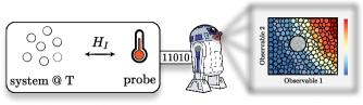
Figure 1: Probe-based thermometry and machine classification. The temperature of a system is estimated by coupling it to a probe, which is subsequently measured. Machine classification uses previously trained data to predict the temperature from experimental observations. Here we use the KNN algorithm, which constructs an observation heat map (right plot) from training set consisting of pairs $(D_{i},T_{i})$, corresponding to $d$-dimensional data $D_{i}$ (here $d=2$) and associated temperatures $T_{i}$.

In this letter we show how machine classification algorithms can be used to provide precise temperature estimation, in a flexible and experimentally friendly way. The scenario we consider is shown in Fig. 1. The temperature $T$ of a system S is measured by first sending a probe P to interact with it, and then measuring the probe. This yields some data $D$, from which we want to construct a reliable estimator $\hat{T}(D)$. Classification accomplishes this by training an algorithm in advance, with a set of points $(D_{i},T_{i})$. This can be obtained from, e.g., computer simulations or a calibration experiment. The result is a predictor function, $\hat{T}(D)$, which can be used to estimate the temperature given any real observation $D$. Classification is a non-parametric technique, and hence is model independent, making it extremely flexible. It accepts any kind of probe observable, and any kind of S-P interaction strategy. Moreover, it is also guaranteed to be asymptotically converge to the true temperature provided the number of training features increased Samworth (2012); Cabannes et al. (2021); Duda et al. (2000).

Machine learning has recently seen an explosion of new applications in physics Das Sarma et al. (2019); Carleo et al. (2019), from quantum phase transitions Carrasquilla and Melko (2017); Rem et al. (2019); Canabarro et al. (2019); Venderley et al. (2018) to quantum dynamics Vicentini et al. (2019); Hartmann and Carleo (2019); Flurin et al. (2020); Mazza et al. (2021); Martina et al. (2021); Fanchini et al. (2021); Innocenti et al. (2020); Bukov (2018); Sgroi et al. (2021) and adaptive estimation Hentschel and Sanders (2010); *Hentschel2011; Lovett et al. (2013); Xu et al. (2019); Schuff et al. (2020); Spagnolo et al. (2019). We will show below that classification in thermometry is robust against many issues commonly faced in realistic thermometry scenarios. First, it naturally handles experimental noise. And second, and most remarkably, it handles cases where other parameters in the process are not known. For instance, we explore the scenario in which the S-P interaction strength is only known to lie within a certain range, which is very reasonable from an experimental point of view. Our methods are illustrated in two experimentally relevant models: impurity thermometry in a Bose-Einstein condensate, and estimation of the thermal phonon number in the Rabi model.

Probe-based thermometry- We consider the setting depicted in Fig. 1. A system S, prepared in a thermal Gibbs state $\rho_{S}=e^{-\beta H_{S}}/Z$, at a certain (unknown) inverse temperature $\beta=1/T$, is coupled to a probe P prepared in an initial state $\rho_{P}$. The total Hamiltonian is taken as $H_{\rm tot}=H_{S}+H_{P}+H_{I}$, where $H_{I}$ is their interaction. The state of the probe after a certain time $t$ will then be given by $\rho_{P}(t)=\mathrm{tr}_{S}\Big{\{}e^{-iH_{\rm tot}t}\big{(}\rho_{S}\otimes\rho_{P})e^{iH_{\rm tot}t}\Big{\}}$, from which information about $T$ can be extracted.

We assume this is accomplished by measuring the expectation values of some probe observables $\langle\mathcal{O}\rangle_{t}:=\mathrm{tr}\big{(}\mathcal{O}\rho_{P}(t)\big{)}$. The uncertainty $\delta T^{2}$ resulting from $\nu$ measurements (obtained in independent repetitions of the experiment) is then Braunstein and Caves (1994); Tóth and Apellaniz (2014); Mehboudi et al. (2018a)

$$\delta T^{2}=\frac{\Delta^{2}\mathcal{O}}{\nu\chi_{T}^{2}(\mathcal{O})},$$ (1)

where $\Delta^{2}O=\langle\mathcal{O}^{2}\rangle_{t}-\langle\mathcal{O}\rangle_{t}^{2}$ and $\chi_{T}^{2}(\mathcal{O})=\partial_{T}\langle\mathcal{O}\rangle_{t}$. Some observables are more sensitive than others; the ultimate precision is determined by the Cramer-Rao bound Braunstein and Caves (1994); Paris (2009)

$$\delta T^{2}\geqslant\frac{1}{\nu\mathcal{F}(T)},$$ (2)

where $\mathcal{F}(T)$ is the Quantum Fisher Information (QFI). When the probe fully thermalizes with the system, the QFI can be written solely in terms of the probe’s energy variance De Pasquale and Stace (2018); Mehboudi et al. (2018b). But in general , the state of the probe is out of equilibrium and the QFI must be determined with the usual quantum metrology tools Paris (2009).

Classification can make use of not only a single observable, but a dataset $D=(\langle\mathcal{O}_{1}\rangle,\ldots,\langle\mathcal{O}_{d}\rangle)$, of dimension $d$. This could mean different observables, or the same observable measured at different times. In either case, each observable is determined from independent experiments. Intuitively speaking, the richer the dataset, the less likely it is that the data was generated from any other temperature than the real one.

The $k$ nearest-neighbors (KNN) algorithm - We introduce the KNN classification algorithm Fix and Hodges (1989); Altman (1992); Duda et al. (2000) as a model-independent (non-parametric) approach to thermometry. Classification is a pattern recognition method . We first train the algorithm using $N$ datasets $(D_{i},T_{i})$ generated from either computer simulations, or a calibration experiment. Each dataset $D_{i}$ is pictured as a point in a $d$-dimensional grid (Fig. 1), which is also labeled by the corresponding temperature $T_{i}$. When an actual observation $D$ arrives, the algorithm locates its position in this grid and computes the Euclidean distance to its $k$ nearest-neighbors. The inverse distances serve as weights to build the probability that $D$ is associated with each $k$ neighbor. The average of said probability yields the estimator $\hat{T}(D)$. And the variance yields the so-called excess risk $\delta T_{\rm exc}^{2}$, which represents the additional uncertainty incurred from using a finite number $N$ of training points (which vanishes if $N\to\infty$). From $\delta T_{\rm exc}$ we can then compute the mean-squared error (MSE), which also takes into account the bias:

$${\rm MSE}(D,T)=\delta T_{\rm exc}^{2}+\Big{(}\hat{T}(D)-T\Big{)}^{2},$$ (3)

with $T$ being the real temperature. The MSE can only be estimated if the true temperature is known in advance. Hence, although it serves as a useful figure of merit, one generally would not have direct access to it in an experiment. The KNN algorithm is asymptotically unbiased Duda et al. (2000); Samworth (2012), so the MSE also vanishes when $N\to\infty$. In the applications below, we have used the KNN implementation in Python from Ref. Pedregosa et al. (2011).

Impurity thermometry in a Bose-Einstein condensate (BEC) - To illustrate the main idea, we start with the experimentally meaningful problem of estimating the temperature of a Bose gas by means of an impurity, for which the BEC acts as a bath Olf et al. (2015); Sabín et al. (2015); Mehboudi et al. (2018a). We follow an approach similar to Mehboudi et al. (2018a); Khan et al. (2021) and consider a Yb impurity (the probe), trapped in a parabolic potential of frequency $\Omega$, and immersed in a K BEC with trap frequency $\omega_{B}$. The solution for the reduced dynamics of the impurity is given in Lampo et al. (2018), and is not restricted to weak coupling. To illustrate the method, we focus on the steady-state fluctuations of the impurity’s position, which reads Lampo et al. (2018)

$$\langle x^{2}\rangle=\frac{\hbar}{2\pi}\int\limits_{-\omega_{B}}^{\omega_{B}}d\omega~{}\coth(\hbar\omega/k_{B}T)\tilde{\chi}^{\prime\prime}(\omega),$$ (4)

where $\tilde{\chi}^{\prime\prime}(\omega)=(\omega\zeta/m_{I})/[(\omega\zeta)^{2}+(\Omega^{2}-\omega^{2}+\omega\theta)^{2}]$ is the impurity’s response function, with $\zeta=\pi\gamma\omega^{3}/2\omega_{B}^{3}$ and $\theta=-(\gamma\omega/2\omega_{B}^{3})[\omega_{B}^{2}+\omega^{2}\ln((\omega_{B}/\omega)^{2}-1)]$. Here, $m_{I}$ is the impurity’s mass and $\gamma$ is a constant proportional to the BEC-impurity interaction strength (see Lampo et al. (2018) for the full Hamiltonian).

We fix $\gamma=30$ Hz, $\omega_{B}=2\Omega=2\pi\times 50$ Hz. As a first test, we assume that $\langle x^{2}\rangle$ can be measured with infinite precision. To train the algorithm, we generate pairs $(D_{i},T_{i})$ with $N$ equally spaced temperatures from $0.1$ nK to $2$ nK. The algorithm is then tested using values of $\langle x^{2}\rangle$ obtained from randomly chosen temperatures within the same interval. Fig. 2(a) shows the predictions $\hat{T}$ as a function of the real temperatures $T$, using only $N=10$ training points. The error bars represent the excess risk $\delta T_{\rm exc}$. In Fig. 2(b) we plot the difference $\hat{T}-T\pm\delta T_{\rm exc}$ for varying sizes $N$ of the training set. Small values of $N$ lead to large uncertainties and systematic biases, specially at the boundaries. But both are rapidly suppressed with increasing $N$.

Next we turn to noisy datasets. In principle, noise could also be included in the training set, e.g. when the data is obtained from another calibration experiment. In the present case, however, the training set is based on the analytical model (4), and is hence error-free. Fig. 2(c) shows the average MSE (3), obtained from $\nu=2000$ independent experiments, for either $N=20$ or $N=100$ training points. We also plot Eq. (1) in gray, and the Cramer-Rao bound (2) in dashed (computed from Correa et al. (2017); Mehboudi et al. (2018a)). The latter can only be reached with special choices of measurement operators Paris (2009); Escher et al. (2011), while Eq. (1) represents the best precision attainable using only measurements of $\langle x^{2}\rangle$ Mehboudi et al. (2018a), as in our case.

When $N=20$, the MSE is significantly above the gray curve, but for $N=100$ both the excess risk $\delta T_{\rm exc}$ and the systematic biases are suppressed, bringing the MSE very close to (1). Our method is thus capable of producing quantitatively precise estimates of $T$. The only exception is the boundaries of the training set. This happens because the fluctuations generate points $\langle x^{2}\rangle$ associated with temperatures outside the interval. In real experiments, it is important to avoid this by ensuring the span of the training set is sufficiently broad. There are also extensions of the KNN algorithm which can monitor whenever a point lies outside the training set, a problem known as anomaly detection Gu et al. (2019); Bergman et al. (2020).

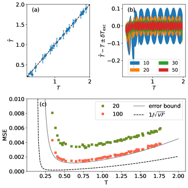
Figure 2: Impurity thermometry of a BEC, focusing on the steady-state position fluctuations (4). (a) Estimator $\hat{T}$ versus the real temperature $T$ using $N=10$ points in the training set. Error bars represent the excess risk $\delta T_{\rm exc}$, and can be suppressed by increasing $N$. This is further shown in (b), which plots $\hat{T}-T\pm\delta T_{\rm exc}$ for different choices of $N$. (c) Average MSE from $\nu=2000$ repetitions of a noisy experiment, for $N=20$ and $N=100$. Gray and black-dashed curves corresponds to Eqs. (1) and (2) respectively. When only $\langle x^{2}\rangle$ is measured, no estimator can improve below the gray curve.

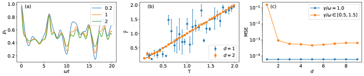
Figure 3: Temperature prediction in the Rabi model. (a) Population $p_{t}$ for $\gamma/\omega=1$ and different values of $k_{B}T/\hbar\omega$. (b) Predicted vs. real temperatures for $d=1,2$. (c) MSE vs. $d$, when $\gamma/\omega$ is known with certainty or when it is only known to lie within a certain interval. The algorithm was trained by generating values of $p_{t}$, with equally spaced tuples of $(T,\gamma)$ in the intervals $[0.1,2]$ and $[0.5,1.5]$, at times $t=0.5,1.0,1.5,2.0,\ldots$. A dataset with e.g. $d=3$ points consists in the array $D=(p_{0.5},p_{1.0},p_{1.5})$.

Rabi model- The previous model served to illustrate how our method can efficiently handle realistic noise in the measurement data. But the model itself was far too simple, as it involved only a single feature $\langle x^{2}\rangle$, which could also be computed analytically. We now turn to a more complicated model with two new ingredients: (i) the dynamics are not analytically soluble; and (ii) the system-probe interaction strength is not known. The latter, in particular, is a very realistic assumption, which is seldom considered in studies of probe-based thermometry. Our algorithm can handle this efficiently using additional features ($d>1$) in the dataset. This combination of flexibility and robustness is the main advantage of our framework.

We illustrate the idea using the Rabi model, which frequently appears in a variety of platforms, from cavity quantum electrodynamics to trapped ions and superconducting circuits. Similar results can also be obtained, e.g., for the Jaynes-Cummings model. The probe is a qubit, with Pauli operators $\sigma_{\pm}$, and the system is a bosonic mode, with annihilation operators $a$. The total Hamiltonian is

$$H=\hbar\omega a^{\dagger}a+\hbar\Omega\sigma_{+}\sigma_{-}+\hbar\gamma(a+a^{\dagger})(\sigma_{+}+\sigma_{-}),$$ (5)

where $\gamma$ is the interaction strength. Estimation of the thermal occupation number of the bosonic mode is one of the most basic problems in e.g., trapped ions Leibfried et al. (2003); Wineland et al. (1998). Quantities are measured in units of $\omega=1$. The probe is taken to be resonant with the system ($\Omega=\omega$) and start in the excited state $\rho_{P}=|1\rangle\langle 1|$. The free parameters are thus the coupling strength $\gamma$, and the system’s initial temperature $T$. We focus on the probe’s populations $p_{t}=\langle\sigma_{+}\sigma_{-}\rangle_{t}$, but the algorithm also works with coherences. Numerically simulated curves of $p_{t}$ vs. $\omega t$, for different $T$, are shown in Fig. 3(a) (c.f. Lv et al. (2017) for experimental results). They serve to illustrate the non-trivial temperature dependence, which would be difficult to fit with standard methods (specially taking into account the computational complexity of simulating the model).

We consider $k_{B}T/\hbar\omega\in[0.1,2]$, and assume $\gamma/\omega$ is only known to lie in the interval $[0.5,1.5]$. Populations were computed numerically for a grid of $100\times 100$ tuples $(T,\gamma)$, and for different times $\omega t=0.5,1.0,1.5,2.0,\ldots$ (other choices of times only marginally affect the results). To analyze the role of the number of features $d$, we adopt the strategy that a dataset with, e.g. $d=3$ consists of $D=(p_{0.5},p_{1},p_{1.5})$, and so on. For simplicity, we also assume all data points are noiseless, as the effects of such noise have already been explored in Fig. 2(c).

Fig. 3(b) shows the results of the estimation when $d=1$ and $d=2$. Since $\gamma$ is not known, using only $d=1$ yields terrible results. But, remarkably, with as little as $d=2$ features, the results are already remarkably good. We explore this further in Fig. 3(c), where the MSE is found to decrease dramatically with increasing $d$ (note the log scale), until saturating at a value that is is ultimately determined by the number of points $N$ in the grid. We also show in Fig. 3(c) the results which would be obtained if $\gamma$ was known with certainty. In this case, the MSE is independent of $d$, with a value once again determined solely by $N$. Thus, with sufficiently many measurements, the precision becomes roughly independent of our uncertainty in the interaction strength.

Thermometric data structures- The results just presented indicate that the use of classification — and the KNN algorithm — in probe-based thermometry is not only versatile, but also robust. Similar tests have also been performed in various other systems, such as qudit models and spin chains. And we have also explored a large variety of parameter choices: e.g., resonant vs. non-resonant energy gaps in Eq. (5), different initial probe states, and so on. Even though the fine details differ from one case to the other, the overall performance is similar in all cases: precise estimation with asymptotically diminishing errors.

We argue that this happens because the probe observables depend smoothly on $T$. Even though the probe is intrinsically out of equilibrium, the spirit is similar to equilibrium quantities, such as energy, entropy or specific heat. It is rare, for instance, to find observables that are oscillatory in $T$, or behave very erratically. Instead, this smooth dependence causes the data structures to be segmented into well-defined regions, which is crucial for the KNN performance. Thermometry thus represents a niche within the realm of parameter estimation, where classification methods could prove to be particularly useful.

To corroborate this argument, we analyze the data structures stemming from the Rabi model (5). Fig. 4 shows curves of $p_{t_{1}}$ vs. $p_{t_{2}}$ for two choices of $(t_{1},t_{2})$. The conditions are similar to those of Figs. 3. As can be seen, irrespective of the value of $\gamma$, points are clearly segmented by temperature, and changes from the hot to the cold regions are always smooth. There are very few regions, for instance, where hot and cold points mix together. This explains why the KNN algorithm is successful. One should also bear in mind that one often uses more than $d=2$ observations, which help to further disentangle the cold and hot regions.

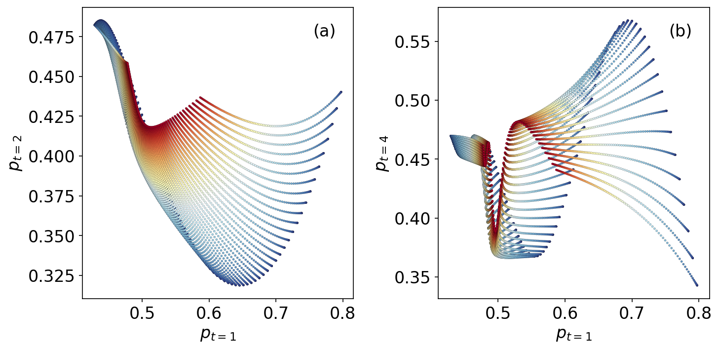
Figure 4: Qubit populations in the Rabi model, $p_{t_{1}}$ vs. $p_{t_{2}}$, for different choices of $(T,\gamma)$, with the color of each point representing the corresponding temperature. (a) $p_{t=2}$ vs. $p_{t=1}$. (b) $p_{t=4}$ vs. $p_{t=1}$.

Significance- We have showed that classification provides a general and flexible platform, that can be applied to any probe-based system. It can accept any kind of observation as input, handles noise in the dataset, and allows the inclusion of additional uncertainties about the model parameters. Moreover, as we have shown, it provides quantitative error assessment and is asymptotically consistent. In light of these facts, we, believe classification may become a useful tool in experimental quantum thermometry. Indeed, several quantum coherent experiments, such as trapped ions and optomechanics, already fall under this category and could directly benefit from this formalism.

Acknowledgements- FFF and GTL acknowledge the financial support of the São Paulo Funding Agency FAPESP (Grants No. 2021/04655-8,  2017/50304-7, 2017/07973-5 and 2018/12813-0) and the Brazilian funding agency CNPq (Grant No. INCT-IQ 246569/2014-0). GTL acknowledges the support from the Eichenwald foundation (Grant No. 0118 999 881 999 119 7253). AOJ acknowledges the financial support from the Foundation for Polish Science through TEAM-NET project (contract no. POIR.04.04.00-00-17C1/18-00). FSL acknowledges financial support of the National Council for Scientific and Technological Development (CNPq) (Grant No. 151435/2020-0).

References

- Giazotto et al. (2006) Francesco Giazotto, Tero T. Heikkilä, Arttu Luukanen, Alexander M. Savin, and Jukka P. Pekola, “Opportunities for mesoscopics in thermometry and refrigeration: Physics and applications,” Reviews of Modern Physics 78, 217–274 (2006).
- Yue and Wang (2012) Yanan Yue and Xinwei Wang, “Nanoscale thermal probing,” Nano Reviews 3, 11586 (2012).
- Onofrio (2016) Roberto Onofrio, “Cooling and thermometry of atomic Fermi gases,” Uspekhi Fizicheskih Nauk 186, 1229–1256 (2016).
- Karimi et al. (2020) Bayan Karimi, Fredrik Brange, Peter Samuelsson, and Jukka P. Pekola, “Reaching the ultimate energy resolution of a quantum detector,” Nature Communications 11, 367 (2020).
- Gasparinetti et al. (2015) S. Gasparinetti, K. L. Viisanen, O.-P. Saira, T. Faivre, M. Arzeo, M. Meschke, and Jukka P. Pekola, “Fast Electron Thermometry for Ultrasensitive Calorimetric Detection,” Physical Review Applied 3, 014007 (2015).
- Sabín et al. (2015) Carlos Sabín, Angela White, Lucia Hackermuller, and Ivette Fuentes, “Impurities as a quantum thermometer for a Bose-Einstein condensate,” Scientific Reports 4, 6436 (2015).
- Marzolino and Braun (2013) Ugo Marzolino and Daniel Braun, “Precision measurements of temperature and chemical potential of quantum gases,” Physical Review A 88, 063609 (2013).
- Mehboudi et al. (2018a) Mohammad Mehboudi, Aniello Lampo, Christos Charalambous, Luis A. Correa, M. A. García-March, and Maciej Lewenstein, “Using polarons for sub- nK quantum non-demolition thermometry in a Bose-Einstein condensate,” Physical Review Letters 122, 030403 (2018a).
- Mitchison et al. (2020) Mark T. Mitchison, Thomás Fogarty, Giacomo Guarnieri, Steve Campbell, Thomas Busch, and John Goold, “In Situ Thermometry of a Cold Fermi Gas via Dephasing Impurities,” Physical Review Letters 125, 080402 (2020).
- Bouton et al. (2020) Quentin Bouton, Jens Nettersheim, Daniel Adam, Felix Schmidt, Daniel Mayer, Tobias Lausch, Eberhard Tiemann, and Artur Widera, “Single-Atom Quantum Probes for Ultracold Gases Boosted by Nonequilibrium Spin Dynamics,” Physical Review X 10, 011018 (2020).
- Neumann et al. (2013) P. Neumann, I. Jakobi, F. Dolde, C. Burk, R. Reuter, G. Waldherr, J. Honert, T. Wolf, A. Brunner, J. H. Shim, D. Suter, H. Sumiya, J. Isoya, and J. Wrachtrup, “High-Precision Nanoscale Temperature Sensing Using Single Defects in Diamond,” Nano Letters 13, 2738–2742 (2013).
- Shim et al. (2021) Jeong Hyun Shim, Seong-Joo Lee, Santosh Ghimire, Ju Il Hwang, Kang Geol Lee, Kiwoong Kim, Matthew J. Turner, Connor A. Hart, Ronald L. Walsworth, and Sangwon Oh, “Multiplexed sensing of magnetic field and temperature in real time using a nitrogen vacancy spin ensemble in diamond,” , 1–8 (2021).
- Halbertal et al. (2016) D. Halbertal, J. Cuppens, M. Ben Shalom, L. Embon, N. Shadmi, Y. Anahory, H. R. Naren, J. Sarkar, A. Uri, Y. Ronen, Y. Myasoedov, L. S. Levitov, E. Joselevich, A. K. Geim, and E. Zeldov, “Nanoscale thermal imaging of dissipation in quantum systems,” Nature 539, 407–410 (2016).
- Mehboudi et al. (2018b) Mohammad Mehboudi, Anna Sanpera, and Luis A. Correa, “Thermometry in the quantum regime: Recent theoretical progress,” (2018b).
- De Pasquale and Stace (2018) Antonella De Pasquale and Thomas M Stace, “Quantum Thermometry,” in Thermodynamics in the quantum regime - Fundamental Aspects and New Directions, edited by F Binder, L. A. Correa, C. Gogolin, J. Anders, and G Adesso (Springer International Publishing, 2018) pp. 1–16.
- Jevtic et al. (2015) Sania Jevtic, David Newman, Terry Rudolph, and T. M. Stace, “Single-qubit thermometry,” Physical Review A - Atomic, Molecular, and Optical Physics 91, 012331 (2015).
- Correa et al. (2015) Luis A. Correa, Mohammad Mehboudi, Gerardo Adesso, and Anna Sanpera, “Individual quantum probes for optimal thermometry,” Physical Review Letters 114, 220405 (2015).
- De Pasquale et al. (2016) Antonella De Pasquale, Davide Rossini, R. Fazio, and Vittorio Giovannetti, “Local quantum thermal susceptibility,” Nature Communications 7, 1–8 (2016).
- Johnson et al. (2016) T. H. Johnson, F. Cosco, Mark T. Mitchison, D. Jaksch, and S. R. Clark, “Thermometry of ultracold atoms via nonequilibrium work distributions,” Physical Review A 93, 053619 (2016).
- Potts et al. (2019) Patrick P. Potts, Jonatan Bohr Brask, and Nicolas Brunner, “Fundamental limits on low-temperature quantum thermometry with finite resolution,” Quantum 3, 161 (2019).
- Mancino et al. (2017) Luca Mancino, Marco Sbroscia, Ilaria Gianani, Emanuele Roccia, and Marco Barbieri, “Quantum Simulation of Single-Qubit Thermometry Using Linear Optics,” Physical Review Letters 118, 130502 (2017).
- Campbell et al. (2017) Steve Campbell, Mohammad Mehboudi, Gabriele De Chiara, and Mauro Paternostro, “Global and local thermometry schemes in coupled quantum systems,” New Journal of Physics 19, 103003 (2017).
- Correa et al. (2017) Luis A. Correa, Martí Perarnau-Llobet, Karen V. Hovhannisyan, Senaida Hernández-Santana, Mohammad Mehboudi, and Anna Sanpera, “Low-temperature thermometry can be enhanced by strong coupling,” Physical Review A - Atomic, Molecular, and Optical Physics 96, 062103 (2017).
- Paris (2016) Matteo G A Paris, “Achieving the Landau bound to precision of quantum thermometry in systems with vanishing gap,” Journal of Physics A: Mathematical and Theoretical 49, 03LT02 (2016).
- Campbell et al. (2018) Steve Campbell, Marco G. Genoni, and Sebastian Deffner, “Precision thermometry and the quantum speed limit,” Quantum Science and Technology 3, 1–7 (2018).
- Wineland et al. (1998) D.J. Wineland, C. Monroe, W.M. Itano, D. Leibfried, B.E. King, and D.M. Meekhof, “Experimental issues in coherent quantum-state manipulation of trapped atomic ions,” Journal of Research of the National Institute of Standards and Technology 103, 259 (1998).
- Leibfried et al. (2003) D. Leibfried, R. Blatt, C. Monroe, and D. Wineland, “Quantum dynamics of single trapped ions,” Reviews of Modern Physics 75, 281–324 (2003).
- Bowen and Milburn (2016) P W Bowen and G. J. Milburn, Quantum Optomechanics (CRC Press, 2016).
- De Pasquale et al. (2017) Antonella De Pasquale, Kazuya Yuasa, and Vittorio Giovannetti, “Estimating temperature via sequential measurements,” Physical Review A 96, 012316 (2017).
- Seah et al. (2019) Stella Seah, Stefan Nimmrichter, Daniel Grimmer, Jader P. Santos, Angeline Shu, Valerio Scarani, and Gabriel T. Landi, “Collisional quantum thermometry,” Physical Review Letters 123, 180602 (2019).
- Shu et al. (2020) Angeline Shu, Stella Seah, and Valerio Scarani, “Surpassing the thermal Cramér-Rao bound with collisional thermometry,” Physical Review A 102, 042417 (2020).
- Hovhannisyan et al. (2021) Karen V. Hovhannisyan, Mathias R. Jørgensen, Gabriel T. Landi, Álvaro M. Alhambra, Jonatan B. Brask, and Martí Perarnau-Llobet, “Optimal Quantum Thermometry with Coarse-Grained Measurements,” PRX Quantum 2, 020322 (2021).
- Rubio et al. (2020) Jesús Rubio, Janet Anders, and Luis A. Correa, “Global Quantum Thermometry,” , 1–9 (2020).
- Alves and Landi (2021) Gabriel O. Alves and Gabriel T. Landi, “Bayesian estimation for collisional thermometry,” , 1–10 (2021).
- Samworth (2012) Richard J. Samworth, “Optimal weighted nearest neighbour classifiers,” Annals of Statistics 40, 2733–2763 (2012).
- Cabannes et al. (2021) Vivien Cabannes, Alessandro Rudi, and Francis Bach, “Fast rates in structured prediction,” 134, 1–43 (2021).
- Duda et al. (2000) Richard O. Duda, Peter E. Hart, and David G. Stork, Pattern classification, 2nd ed. (Wiley, New York, 2000) p. 688.
- Das Sarma et al. (2019) Sankar Das Sarma, Dong-Ling Deng, and Lu-Ming Duan, “Machine learning meets quantum physics,” Physics Today 72, 48–54 (2019).
- Carleo et al. (2019) Giuseppe Carleo, Ignacio Cirac, Kyle Cranmer, Laurent Daudet, Maria Schuld, Naftali Tishby, Leslie Vogt-Maranto, and Lenka Zdeborová, “Machine learning and the physical sciences,” Reviews of Modern Physics 91, 045002 (2019).
- Carrasquilla and Melko (2017) Juan Carrasquilla and Roger G. Melko, “Machine learning phases of matter,” Nature Physics 13, 431–434 (2017).
- Rem et al. (2019) Benno S Rem, Niklas Käming, Matthias Tarnowski, Luca Asteria, Nick Fläschner, Christoph Becker, Klaus Sengstock, and Christof Weitenberg, “Identifying quantum phase transitions using artificial neural networks on experimental data,” Nature Physics 15, 917–920 (2019).
- Canabarro et al. (2019) Askery Canabarro, Felipe Fernandes Fanchini, André Luiz Malvezzi, Rodrigo Pereira, and Rafael Chaves, “Unveiling phase transitions with machine learning,” Physical Review B 100, 045129 (2019).
- Venderley et al. (2018) Jordan Venderley, Vedika Khemani, and Eun Ah Kim, “Machine Learning Out-of-Equilibrium Phases of Matter,” Physical Review Letters 120, 257204 (2018).
- Vicentini et al. (2019) Filippo Vicentini, Alberto Biella, Nicolas Regnault, and C. Ciuti, “Variational Neural-Network Ansatz for Steady States in Open Quantum Systems,” Physical Review Letters 122, 250503 (2019).
- Hartmann and Carleo (2019) Michael J. Hartmann and Giuseppe Carleo, “Neural-Network Approach to Dissipative Quantum Many-Body Dynamics,” Physical Review Letters 122, 250502 (2019).
- Flurin et al. (2020) E Flurin, L. S. Martin, S. Hacohen-Gourgy, and I Siddiqi, “Using a Recurrent Neural Network to Reconstruct Quantum Dynamics of a Superconducting Qubit from Physical Observations,” Physical Review X 10, 011006 (2020).
- Mazza et al. (2021) Paolo P. Mazza, Dominik Zietlow, Federico Carollo, Sabine Andergassen, Georg Martius, and Igor Lesanovsky, “Machine learning time-local generators of open quantum dynamics,” Physical Review Research 3, 023084 (2021).
- Martina et al. (2021) Stefano Martina, Stefano Gherardini, and Filippo Caruso, “Machine learning approach for quantum non-Markovian noise classification,” , 1–14 (2021).
- Fanchini et al. (2021) Felipe F. Fanchini, Göktuğ Karpat, Daniel Z. Rossatto, Ariel Norambuena, and Raúl Coto, “Estimating the degree of non-Markovianity using machine learning,” Physical Review A 103, 022425 (2021).
- Innocenti et al. (2020) Luca Innocenti, Leonardo Banchi, Alessandro Ferraro, Sougato Bose, and Mauro Paternostro, “Supervised learning of time-independent Hamiltonians for gate design,” New Journal of Physics 22, 065001 (2020).
- Bukov (2018) Marin Bukov, “Reinforcement learning for autonomous preparation of Floquet-engineered states: Inverting the quantum Kapitza oscillator,” Physical Review B 98, 224305 (2018).
- Sgroi et al. (2021) Pierpaolo Sgroi, G. Massimo Palma, and Mauro Paternostro, “Reinforcement Learning Approach to Nonequilibrium Quantum Thermodynamics,” Physical Review Letters 126, 020601 (2021).
- Hentschel and Sanders (2010) Alexander Hentschel and Barry C. Sanders, “Machine Learning for Precise Quantum Measurement,” Physical Review Letters 104, 063603 (2010).
- Hentschel and Sanders (2011) Alexander Hentschel and Barry C. Sanders, “Efficient Algorithm for Optimizing Adaptive Quantum Metrology Processes,” Physical Review Letters 107, 233601 (2011).
- Lovett et al. (2013) Neil B. Lovett, Cécile Crosnier, Martí Perarnau-Llobet, and Barry C. Sanders, “Differential Evolution for Many-Particle Adaptive Quantum Metrology,” Physical Review Letters 110, 220501 (2013).
- Xu et al. (2019) Han Xu, Junning Li, Liqiang Liu, Yu Wang, Haidong Yuan, and Xin Wang, “Generalizable control for quantum parameter estimation through reinforcement learning,” npj Quantum Information 5, 82 (2019).
- Schuff et al. (2020) Jonas Schuff, Lukas J. Fiderer, and Daniel Braun, “Improving the dynamics of quantum sensors with reinforcement learning,” New Journal of Physics 22, 035001 (2020).
- Spagnolo et al. (2019) Nicolò Spagnolo, Alessandro Lumino, Emanuele Polino, Adil S. Rab, Nathan Wiebe, and Fabio Sciarrino, “Machine Learning for Quantum Metrology,” Proceedings 12, 28 (2019).
- Braunstein and Caves (1994) Samuel L. Braunstein and Carlton M. Caves, “Statistical distance and the geometry of quantum states,” Physical Review Letters 72, 3439–3443 (1994).
- Tóth and Apellaniz (2014) Géza Tóth and Iagoba Apellaniz, “Quantum metrology from a quantum information science perspective,” Journal of Physics A: Mathematical and Theoretical 47, 424006 (2014).
- Paris (2009) Matteo G.A. Paris, “Quantum Estimation for Quantum Technology,” International Journal of Quantum Information 7, 125 (2009).
- Fix and Hodges (1989) Evelyn Fix and J. L. Hodges, “Discriminatory Analysis. Nonparametric Discrimination: Consistency Properties,” International Statistical Review / Revue Internationale de Statistique 57, 238 (1989).
- Altman (1992) N S Altman, “An Introduction to Kernel and Nearest-Neighbor Nonparametric Regression,” The American Statistician 46, 175 (1992).
- Note (1) Other methods, such as neural networks, were also tested, but presented no visible advantages.
- Pedregosa et al. (2011) Fabian Pedregosa, Gael Varoquaux, Alexandre Gramfort, Vincent Michel, Bertrand Thirion, Olivier Grisel, Mathieu Blondel, Peter Prettenhofer, Ron Weiss, Vincent Dubourg, Jake Vanderplas, Alexandre Passos, David Cournapeau, Matthieu Brucher, Matthieu Perrot, and Édouard Duchesnay, “Scikit-learn: Machine learning in Python,” Journal of Machine Learning Research 12, 2825–2830 (2011).
- Olf et al. (2015) Ryan Olf, Fang Fang, G. Edward Marti, Andrew MacRae, and Dan M. Stamper-Kurn, “Thermometry and cooling of a Bose gas to 0.02 times the condensation temperature,” Nature Physics 11, 720–723 (2015).
- Khan et al. (2021) Muhammad Miskeen Khan, Mohammad Mehboudi, Hugo Tercas, Maciej Lewenstein, and Miguel-Angel Garcia-March, “Sub-nK thermometry of an interacting $d$-dimensional homogeneous Bose gas,” , 1–12 (2021).
- Lampo et al. (2018) Aniello Lampo, Christos Charalambous, Miguel Ángel García-March, and MacIej Lewenstein, “Non-Markovian polaron dynamics in a trapped Bose-Einstein condensate,” Physical Review A 98, 063630 (2018).
- Escher et al. (2011) B. M. Escher, R. L. De Matos Filho, and L. Davidovich, “General framework for estimating the ultimate precision limit in noisy quantum-enhanced metrology,” Nature Physics 7, 406–411 (2011).
- Gu et al. (2019) Xiaoyi Gu, Leman Akoglu, and Alessandro Rinaldo, “Statistical analysis of nearest neighbor methods for anomaly detection,” Advances in Neural Information Processing Systems 32, 1–11 (2019).
- Bergman et al. (2020) Liron Bergman, Niv Cohen, and Yedid Hoshen, “Deep Nearest Neighbor Anomaly Detection,” (2020).
- Lv et al. (2017) Dingshun Lv, Shuoming An, Zhenyu Liu, Jing-Ning Zhang, Julen S. Pedernales, Lucas Lamata, Enrique Solano, and Kihwan Kim, “Quantum simulation of the quantum Rabi model in a trapped ion,” Physical Review X 8, 21027 (2017).