Fast compression of MCMC output

Abstract

We propose cube thinning, a novel method for compressing the output of a MCMC (Markov chain Monte Carlo) algorithm when control variates are available. It amounts to resampling the initial MCMC sample (according to weights derived from control variates), while imposing equality constraints on averages of these control variates, using the cube method of Deville, (2004). Its main advantage is that its CPU cost is linear in $N$, the original sample size, and is constant in $M$, the required size for the compressed sample. This compares favourably to Stein thinning (Riabiz et al.,, 2020), which has complexity $\mathcal{O}(NM^{2})$, and which requires the availability of the gradient of the target log-density (which automatically implies the availability of control variates). Our numerical experiments suggest that cube thinning is also competitive in terms of statistical error.

1 Introduction

MCMC (Markov chain Monte Carlo) remains to this day the most popular approach to sampling from a target distribution $p$, in particular in Bayesian computation (Robert and Casella,, 2004).

Standard practice is to run a single chain, $X_{1},\ldots,X_{N}$ according to a Markov kernel that leaves invariant $p$. It is also common to discard part of the simulated chain, either to reduce its memory footprint, or to reduce the CPU cost of later post-processing operations, or more generally for the user’s convenience. Historically, the two common recipes for compressing MCMC output are:

• burn-in, which amounts to discarding the $b$ first states; and

• thinning, which amounts to retaining only one out of $t$ (post burn-in) states.

The impact of either recipes on the statistical properties of the sub-sampled estimates are markedly different. Burn-in reduces the bias introduced by the discrepancy between $p$ and the distribution of the initial state $X_{1}$ (since $X_{b}\approx p$ for $b$ large enough). On the other hand, thinning always increases the (asymptotic) variance of MCMC estimates (Geyer,, 1992).

Practitioners often choose $b$ (the burn-in period) and $t$ (the thinning frequency) separately, in a somewhat ad-hoc fashion (i.e. through visual inspection of the initial chain), or using convergence diagnosis such as e.g. those reviewed in Cowles and Carlin, (1996).

Two recent papers (Mak and Joseph,, 2018; Riabiz et al.,, 2020), cast a new light on the problem of compressing a MCMC chain by considering more generally the problem, for a given $M$, of selecting the subsample of size $M$ that best represents (according to a certain criterion) the target distribution $p$. We focus for now on Riabiz et al., (2020), for reasons we explain below.

Stein thinning, the method developed in Riabiz et al., (2020), chooses the sub-sample $\mathcal{S}$ of size $M$ which minimises the following criterion:

$$D(\mathcal{S}):=\frac{1}{M^{2}}\sum_{m,n\in\mathcal{S}}k_{p}(X_{m},X_{n}),\quad\mathcal{S}\subset\{1,\ldots,N\},\quad|\mathcal{S}|=M$$ (1)

where $k_{p}$ is a $p-$dependent kernel function derived from another kernel function $k:\mathcal{X}\times\mathcal{X}\rightarrow\mathbb{R}$, as follows:

$$k_{p}(x,y)=\nabla_{x}\cdot\nabla_{y}k(x,y)+\langle\nabla_{x}k(x,y),s_{p}(y)\rangle\\ +\langle\nabla_{y}k(x,y),s_{p}(x)\rangle+k(x,y)\langle s_{p}(x),s_{p}(y)\rangle$$

with $\langle\cdot,\cdot\rangle$ being the Euclidean inner product, $s_{p}(x):=\nabla\log p(x)$ is the so-called score function (gradient of the log target density), and $\nabla$ the gradient operator.

The rationale behind criterion (1) is that it may be interpreted as the KSD (kernel Stein divergence) between the true distribution $p$ and the empirical distribution of sub-sample $S$. We refer to Riabiz et al., (2020) for more details on the theoretical background of the KSD, and its connection to Stein’s method.

Stein thinning is appealing, as it seems to offer a principled, quasi-automatic way to compress MCMC output. However, closer inspection reveals the following three limitations.

First, it requires computing the gradient of the log-target density, $s_{p}(x)=\nabla\log p(x)$. This restricts the method to problems where this gradient exists and is tractable (and, in particular, to $\mathcal{X}=\mathbb{R}^{d}$).

Second, its CPU cost is $\mathcal{O}(NM^{2})$. This makes it nearly impossible to use Stein thinning for $M\gg 100$. This cost stems from the greedy algorithm proposed in Riabiz et al., (2020), see their Algorithm 1, which adds at iteration $t$ the state $X_{i}$ which minimises $k_{p}(X_{i},X_{i})+\sum_{j\in S_{t-1}}k_{p}(X_{i},X_{j})$, where $S_{t-1}$ is the sample obtained from the $t-1$ previous iterations.

Third, its performance seems to depend in a non-trivial way on the original kernel function $k$; Riabiz et al., (2020) propose several strategies for choosing and scaling $k$, but none of them seems to perform uniformly well in their numerical experiments.

We propose a different approach in this paper, which we call cube thinning, and which addresses these shortcomings to some extent. Assuming the availability of $J$ control variates (that is, of functions $h_{j}$ with known expectation under $p$), we cast the problem of MCMC compression as that of resampling the initial chain under constraints based on these control variates. The main advantage of cube thinning is that its complexity is $\mathcal{O}(NJ^{3})$; in particular it does not depend on $M$. That makes it possible to use it for much larger values of $M$. (We shall discuss the choice of $J$, but, by and large, $J$ should be of the same order as $d$, the dimension of the sampling space). The name stems from the cube method of Deville, (2004), which plays a central part in our approach, as we explain in the body of the paper.

The availability of control variates may seem like a strong requirement. However, if we assume we are able to compute $s_{p}(x)=\nabla\log p(x)$, then (for a large class of functions $\phi:\mathbb{R}^{d}\rightarrow\mathbb{R}^{d}$, which we define later)

$$\mathbb{E}_{p}\left[\phi(x)s_{p}(x)+\nabla_{x}\cdot\phi(x)\right]=0$$

where $\nabla_{x}\cdot\phi$ denotes the divergence of $\phi$. In other words, the availability of the score function implies automatically the availability of control variates. The converse is not true: there exists control variates (e.g. Dellaportas and Kontoyiannis,, 2011) that are not gradient-based. One of the examples we consider in our numerical examples feature such non gradient-based control variates; as a result, we are able to apply cube thinning, although Stein thinning is not applicable.

The support point methods of Mak and Joseph, (2018) does not require control variates. It is thus more generally applicable than either cube thinning or Stein thinning. On the other hand, when gradients (and thus control variates) are available, the numerical experiments of Riabiz et al., (2020) suggest that Stein thinning outperforms support points. From now on, we focus on situations where control variates are available.

The paper is organised as follows. Section 2.3 recalls the concept of control variates, and explains how control variates may be used to reweight a MCMC sample. Section 3 describes the cube method of Deville, (2004). Section 4 explains how to combine control variates and the cube method to perform cube thinning. Section 5 assesses the statistical performance of cube thinning through two numerical experiments.

We use the following notations throughout: $p$ denotes both the target distribution and its probability density; $p(f)$ is a short-hand for the expectation of $f(X)$ under $p$. The gradient of a function $f$ is denoted by $\nabla_{x}f(x)$, or simply $\nabla f(x)$ when there is no ambiguity. The $i-$th component of a vector $v\in\mathbb{R}^{d}$ is denoted by $v[i]$, and its transpose by by $v^{t}$. The vectors of the canonical basis of $\mathbb{R}^{d}$ are denoted by $e_{i}$, i.e. $e_{i}[j]=1$ if $j=i$, 0 otherwise. Matrices are written in upper-case; the kernel (null space) of matrix $A$ is denoted by $\mathrm{ker}A$. The set of functions $f:\Omega\rightarrow\mathbb{R}^{d}$ that are continuously differentiable is denoted by $C^{1}(\omega,\mathbb{R}^{d})$.

2 Control variates

2.1 Definition

Control variates are a very well known way to reduce the variance of Monte Carlo estimates; see e.g. the books of Robert and Casella, (2004), Glasserman, (2004) and Owen, (2013).

Suppose we want to estimate the quantity $p(f)=\mathbb{E}_{p}[f(X)]$ for a suitable $f:\mathbb{R}^{d}\rightarrow\mathbb{R}$, based on an IID (independent and identically distributed) sample $\{X_{1},\dots,X_{N}\}$ from distribution $p$. (The generalisation of control variates to MCMC will be discussed in Section 4.)

The usual Monte Carlo estimate of $p(f)$ is

$$\hat{p}(f)=\dfrac{1}{N}\sum_{n=1}^{N}f(X_{n}).$$ (2)

Assume we know $J\in\mathbb{N}^{\star}$ functions $h_{j}:\mathbb{R}^{d}\rightarrow\mathbb{R}$ for $j\in\{1,\dots,J\}$ such that $p(h_{j})=0$. Functions with this property are called control variates. We can use this property to build an estimate with a lower variance: let’s denote $h(X)=(h_{1}(X),\dots,h_{J}(X))^{t}$ and write our new estimate:

$$\hat{p}_{\beta}(f)=\dfrac{1}{N}\sum_{n=1}^{N}f(X_{n})+\beta^{t}h(X_{n})$$ (3)

with $\beta\in\mathbb{R}^{J}$. Then it is straightforward to show that $\mathbb{E}[\hat{p}_{\beta}(f)]=\mathbb{E}[\hat{p}(f)]=p(f)$. Depending on the choice of $\beta$ we may have $\mathrm{Var}[\hat{p}_{\beta}(f)]\leq\mathrm{Var}[\hat{p}(f)]$. The next section discusses how to choose such a $\beta$.

2.2 Control variates as a weighting scheme

The standard approach to choose $\beta$ consists of two steps. First, one shows easily that the value the minimises the variance of estimator (3) is:

$$\beta^{\star}(f)=\mathrm{Var}(h(X))^{-1}\mathrm{Cov}(h(X),f(X))$$ (4)

where $\mathrm{Var}(h(X))$ is the $J\times J$ variance matrix of the vector $h(X)$ and $\mathrm{Cov}(h(X),f(X))$ is the $J\times 1$ vector such that $\mathrm{Cov}(h(X),f(X))_{i,1}=\mathrm{Cov}(f(X),h_{i}(X))$.

Second, one realises that this quantity may be estimated from the sample $X_{1},\ldots,X_{N}$ through a simple linear regression model, where the $f(X_{n})$’s are the outcome, and the $h_{j}(X_{n})$’s are the predictors:

$$f(X_{n})\approx\mu+\beta^{t}h(X_{n})+\epsilon_{n},\quad\mathbb{E}[\epsilon_{n}]=0.$$ (5)

More precisely, let $\gamma\in R^{J+1}$ be the vector such that $\gamma^{t}=(\mu,\beta^{t})$, $H=(H_{ij})$ the design matrix such that $H_{i1}=1$, $H_{i(j+1)}=h_{j}(X_{i})$, and $F=(f(X_{1}),\ldots,f(X_{N}))$. Then the OLS (ordinary least squares) estimate of $\gamma$ is

$$\widehat{\gamma}_{\mathrm{OLS}}=(H^{t}H)^{-1}H^{t}F.$$ (6)

Since $\mathbb{E}[f(X_{n})]=\mu$ in this artificial regression model, the first component of $\widehat{\gamma}_{\mathrm{OLS}}$:

$$\hat{p}_{\star}(f):=\widehat{\gamma}_{\mathrm{OLS}}\times e_{1},$$ (7)

actually corresponds to estimate (3) when $\beta=\widehat{\beta}_{\mathrm{OLS}}$.

At first glance, the approach described above seems to require implementing a different linear regression for each function $f$ of interest. Owen, (2013) noted however that one may re-express (7) as a weighted average:

$$\hat{p}_{\star}(f)=\sum_{n=1}^{N}w_{n}f(X_{n})$$ (8)

where the weights $w_{n}$ sum to one, and do not depend on $f$. It is thus possible to compute these weights once from a given sample (given a certain choice of control variates), and then quickly compute $\hat{p}_{\star}(f)$ for any function $f$ of interest.

The exact expression of the weights are easily deduced from (7) and (6): $w=(w_{n})$ with

$$w=H(H^{t}H)^{-1}e_{1}.$$

2.3 Gradient-based control variates

In this section and the next, we recall generic methods to construct control variates. This section considers specifically control variates that derives from the score function, $s_{p}(x)=\nabla\log p(x)$. (We therefore assume that this quantity is tractable.)

Under the following two conditions:

1. the probability density $p\in C^{1}(\Omega,\ R)$ where $\Omega\subseteq\mathbb{R}^{d}$ is an open set;

2. Function $\phi\in C^{1}(\Omega,\mathbb{R}^{d})$ is such that $\oint_{\partial\Omega}p(x)\phi(x)\cdot n(x)S(dx)=0$ where $\oint_{\partial\Omega}$ denotes the integral over the boundary of $\Omega$, and $S(dx)$ is the surface element at $x\in\partial\Omega$;

the following function:

$$h(x)=\nabla_{x}\cdot\phi(x)+\phi(x)\cdot s_{p}(x)$$ (9)

is a control variate: $p(h)=0$, see e.g. Mira et al., (2013) or Oates et al., (2016) for further details. To get some intuition, note that in dimension 1 and assuming the domain of integration is an interval $]a,b[\subset\mathbb{R}$, this amounts to an integration by part with the condition that $h(b)p(b)-h(a)p(a)=0$.

Thus, whenever the score function is available (and the conditions above hold), we are able to construct an infinite number of control variates (one for each function $\phi$). For simplicity, we shall focus on the following standard classes of such functions. First, for $i=1,\ldots,d$,

$$\phi_{i}\colon\mathbb{R}^{d} \rightarrow\mathbb{R}^{d}$$

$$x \mapsto e_{i}$$

which leads to the following $d$ control variates:

$$h_{i}(x)=s_{p}(x)[i].$$ (10)

For a Gaussian target, $N(\mu,\Sigma)$, the score is $s_{p}(x)=-\Sigma^{-1}(x-\mu)$, and the control variates above make it possible to reweigh the Monte Carlo sample to make it have the same expectation as the target distribution.

Second, we consider, for $i,j=1,\ldots,d$:

$$\phi_{ij}\colon\mathbb{R}^{d} \rightarrow\mathbb{R}^{d}$$

$$x \mapsto x[i]e_{j}$$

which leads to the following $d^{2}$ control variates:

$$h_{ij}(x)=\mathds{1}\{i=j\}+x[i]s_{p}(x)[j].$$ (11)

Again, for a Gaussian target $N(\mu,\Sigma)$, this makes it possible to fix the empirical covariance matrix to true covariance $\Sigma$.

In our simulations, we consider two sets of control variates: the ‘full’ set, consisting of the $d$ control variates defined by (10), and the $d^{2}$ control variates defined by (11). And a ‘diagonal’ set of $2d$ control variates, where for (11), we only consider the cases where $i=j$. Of course, the former set should lead to better performance (lower variance), but since the complexity of our approach will be $\mathcal{O}(J^{3})$, where $J$ is the number of control variates, taking $J=\mathcal{O}(d^{2})$ may be too expensive whenever the dimension $d$ is large.

2.4 MCMC-based control variates

We mention in passing other ways to construct control variates, in particular in the context of MCMC.

For instance, Dellaportas and Kontoyiannis, (2011) noted that, for a Markov chain $\{X_{n}\}$, the quantity

$$\phi(X_{n})-\mathbb{E}\left[\phi(X_{n})|X_{n=1}\right]$$

has expectation zero. In particular, if the MCMC kernel is a Gibbs sampler, it is likely that one is able to compute the conditional expectation of each component; i.e. $\phi(x)=x[i]$ for $i=1,\ldots,d$.

See also Hammer and Tjelmeland, (2008) for another way to construct control variates when the $X_{n}$’s are simulated from a Metropolis kernel.

3 The cube method

We review in this section the cube method of Deville, (2004). This method originated from survey sampling, and is a way to sample from a finite population under constraints. The first subsection gives some definitions, the second one explains the flight phase of the cube method and the third subsection discusses the landing phase of the method.

3.1 Definitions

Suppose we have a finite population $\{1,\dots,N\}$ of $N$ individuals and that to each individual $n=1,\ldots,N$ is associated a variable of interest $y_{n}$ and $J$ auxiliary variables, $v_{n}=(v_{n1},\dots,v_{nJ})$. Without loss of generality, suppose also that the $J$ vectors $(v_{1j},\dots,v_{Nj})$ are linearly independent. We are interested in estimating the quantity $Y=\sum_{n=1}^{N}y_{n}$ using a subsample of $\{1,\ldots,N\}$. Furthermore, we know the exact value of each sum $V_{j}=\sum_{n=1}^{N}v_{nj}$, and we wish to use this auxiliary information to better estimate $Y$.

We assign, to each individual $n$, a sampling probability $\pi_{n}\in[0,1]$. We consider random variables $S_{n}$ such that, marginally, $\mathbb{P}(S_{n}=1)=\pi_{n}$. We may then define the Horvitz-Thompson estimator of $Y$:

$$\hat{Y}=\sum_{n=1}^{N}\frac{S_{n}y_{n}}{\pi_{n}}$$ (12)

which is unbiased, and which depends only on selected individuals (i.e $S_{n}=1$).

We define similarly the Horvitz-Thompson estimator of $V_{j}$:

$$\hat{V}_{j}=\sum_{n=1}^{N}\frac{S_{n}v_{nj}}{\pi_{n}}.$$ (13)

Our objective is to construct a joint distribution $\xi$ for the inclusion variables $S_{n}$ such that $\mathbb{P}_{\xi}(S_{n}=1)=\pi_{n}$ for all $n=1,\ldots,N$, and

$$\hat{V}=V\quad\mbox{$\xi$-almost surely.}$$ (14)

where $V=(V_{1},\ldots,V_{J})$, $\hat{V}=(\hat{V}_{1},\ldots,\hat{V}_{J})$. Such a probability distribution is called a balanced sampling design.

3.2 Subsamples as vertices

We can view all the possible samples from $\{1,\ldots,N\}$ as the vertices of the hypercube $\mathcal{C}=[0,1]^{N}$ in $\mathbb{R}^{N}$. A sampling design with inclusion probabilities $\pi_{n}=\mathbb{P}_{\xi}(S_{n}=1)$ is then a distribution over the set of these vertices such that $\mathbb{E}[S]=\pi$, where $S=(S_{1},\ldots,S_{N})^{t}$, and $\pi=(\pi_{1},\ldots,\pi_{N})^{t}$ is the vector of inclusion probabilities. Hence, $\pi$ is expressed as a convex combination of the vertices of the hypercube.

We can think of a sampling algorithm as finding a way to reach any vertex of the cube, starting at $\pi$, while satisfying the balancing equation (14). But before we describe such a sampling algorithm, we may wonder if it is possible to find a vertex such that (14) is satisfied.

3.3 Existence of a solution

The balancing equation (14) defines a linear system. Indeed, we can re-express (14) as $S$ being a solution to $As=V$, where $A=(A_{jn})$ is of dimension $J\times N$, $A_{jn}=v_{kn}/\pi_{n}$. This system defines a hyperplane $Q$ of dimension $N-J$ in $\mathbb{R}^{N}$.

What we want is to find vertices of the hypercube $\mathcal{C}$ that also belong to the hyperplane $Q$. Unfortunately, it is not necessarily possible, as it depends on how the hyperplane $Q$ intersects the cube $\mathcal{C}$. In addition, there is no way to know beforehand if such a vertex exists. Since $\pi\in Q$, we know that $\mathcal{K}:=\mathcal{C}\cap Q\neq\emptyset$ and is of dimension $N-J$. The only thing we can say is stated Proposition 1 in Deville, (2004): if $r$ is a vertex of $\mathcal{K}$, then in general $q=\mathrm{card}(\{n:\,0<r[n]<1\})\leq J$.

The next section describes the flight phase of the cube algorithm, which generates a vertex in $\mathcal{K}$ when such vertices exist, or which, alternatively, returns a point in $\mathcal{K}$ with most (but not all) components set to zero or one. In the latter case, one needs to implement a landing phase, which is discussed in Section 3.5.

3.4 Flight phase

The flight phases simulates a process $\pi(t)$ which takes values in $\mathcal{K}=\mathcal{C}\cap Q$, and starts at $\pi(0)=\pi$. At every time $t$, one selects a unit vector $u(t)$, then one chooses randomly between one of the two points that are in the intersection of the hyper-cube $\mathcal{C}$ and the line parallel to $u(t)$ that passes through $\pi(t-1)$. The probability of selecting these two points are set to ensure that $\pi(t)$ is a martingale; in that way, we have $\mathbb{E}[\pi_{t}]=\pi$ at every time step. The random direction $u(t)$ must be generated to fulfil the following two requirements: (a) that the two points are in $Q$; i.e. $u(t)\in\mathrm{ker}A$; and (b) whenever $\pi(t)$ has reached one of the faces of the hyper-cube, it must stay within that face; thus, $u(t)[k]=0$ if $\pi(t-1)[k]=0$ or $1$.

Algorithm 1 describes one step of the flight phase.

Input: $\pi(t-1)$

Output: $\pi(t)$

1 Sample $u(t)$ in $\ker A$ with $u_{k}(t)=0$ if the $k$-th component of $\pi(t-1)$ is an integer.

2Compute $\lambda^{\star}_{1}$ and $\lambda^{\star}_{2}$, the largest values of $\lambda_{1}>0$ and $\lambda_{2}>0$ such that: $0\leq\pi(t-1)+\lambda_{1}u(t)\leq 1$ and $0\leq\pi(t-1)-\lambda_{2}u(t)\leq 1$.

3With probability $\lambda_{2}^{\star}/(\lambda_{1}^{\star}+\lambda_{2}^{\star})$, set $\pi(t)\leftarrow\pi(t-1)+\lambda_{1}u(t)$; otherwise, set $\pi(t)\leftarrow\pi(t-1)-\lambda_{2}u(t)$.

Algorithm 1 Flight phase iteration

The flight phase stops when Step 1 of Algorithm 1 cannot be performed (i.e. no vector $u(t)$ fulfils these conditions). Until this happens, each iteration increases by at least one the number of components in $\pi(t)$ that are either zero or one. Thus, the flight phases completes at most in $N$ steps.

In practice, to generate $u(t)$, one may proceed as follows: first generate a random vector $v(t)\in\mathbb{R}^{N}$, then project it in the constraint hyperplane: $u(t)=I(t)v(t)-I(t)A^{t}(AI(t)A^{t})^{-}AI(t)v(t)$ where $I(t)$ is a diagonal matrix such that $I_{kk}(t)$ is 0 if $\pi_{k}(t)$ is an integer and 1 otherwise, and $M^{-}$ denotes the pseudo-inverse of the matrix $M$.

Chauvet and Tillé, (2006) propose a particular method to generate vector $v(t)$ which ensures that the complexity of a single iteration of the flight phase is $\mathcal{O}(J^{3})$. This leads to an overall complexity of $\mathcal{O}(NJ^{3})$ for the flight phase, since it terminates in at most $N$ iterations.

3.5 Landing phase

Denote by $\pi^{\star}$ the value of process $\pi(t)$ when the flight phase terminates. If $\pi^{\star}$ is a vertex of $\mathcal{C}$ (i.e. all its components are either zero or one), one may stop and return $\pi^{\star}$ as the output of the cube algorithm. If $\pi^{\star}$ is not a vertex, this informs us that no vertex belongs to $\mathcal{K}$. One may implement a landing phase, which aims at choosing randomly a vertex which is close to $\pi^{\star}$, and such that the variance of the components of $\hat{V}$ is small.

Appendix A gives more details on the landing phase. Note that its worst-case complexity is $\mathcal{O}(2^{J})$. However, in practice, it is typically either much faster, or not required (i.e. $\pi^{\star}$ is already a vertex) as soon as $J\ll N$.

4 Cube thinning

We now explain how the previous ingredients (control variates, and the cube method) may be combined in order to thin a Markov chain, $X_{1},\ldots,X_{N}$, into a sub-sample of size $M$. As before, the invariant distribution of the chain is denoted by $p$, and we assume we know of $J$ control variates $h_{j}$, i.e. $p(h_{j})=0$ for $j=1,\ldots,J$.

4.1 First step: computing the weights

The first step of our method is to use the $J$ control variates to compute the $N$ weights $w_{n}$, as defined at the end of Section 2.2. Recall that these weights sum to one, that they automatically fulfil the constraints:

$$\sum_{n=1}^{N}w_{n}h_{j}(X_{n})=0$$ (15)

for $j=1,\ldots,J$, and that we use them to compute

$$\hat{p}_{\star}(f)=\sum_{n=1}^{N}w_{n}f(X_{n})$$ (16)

as a low-variance estimate for $p(f)$ for any $f$.

Recall that the control variates procedure we described in Section 2 assume that the input variables, $X_{1},\ldots,X_{N}$, are IID. This is obviously not the case in a MCMC context; however, we follow the common practice (Mira et al.,, 2013; Oates et al.,, 2016) of applying the procedure to MCMC points as if they were IID points. This implies that the weighted estimate above corresponds to a value of $\beta$ in (3) that does not minimise the (asymptotic) variance of estimator (3). It is actually possible to estimate the value of $\beta$ that minimises the asymptotic variance of a MCMC estimate (Dellaportas and Kontoyiannis,, 2011; Brosse et al.,, 2019). However, this type of approach is specific to certain MCMC samplers, and, critically for us, it cannot be cast as a weighting scheme. Thus we stick to this standard approach.

We note in passing that, in our experiments (see Figure 1 and the surrounding discussion) the weights $w_{n}$ makes it easy to assess visually the convergence (and thus the burn-in) of the Markov chain. In fact, since the MCMC points of the burn-in phase are far from the mass of the target distribution, the procedure must assign a small or negative weight to these points in order to respect the constraints based on the control variates. Again, see Section 5.2 for more discussion on this issue. The fact that control variates may be used to assess MCMC convergence has been known for a long time (e.g. Brooks and Gelman,, 1998), but the visualisation of weights makes this idea more expedient.

4.2 Second step: cube resampling

The second step consists in resampling the weighted sample $(w_{n},X_{n})_{n=1,\ldots,N}$, to obtain a sub-sample $\mathcal{S}=\{X_{n}:\,S_{n}=1\}$ where $S_{n}$ are random variables such that (a) $\mathbb{E}[S_{n}]=w_{n}$; (b) $\sum_{n=1}^{N}S_{n}=M$, and (c) for $j=1,\ldots,J$:

$$\sum_{S_{n}=1}h_{j}(X_{n})=0.$$

Condition (a) ensures that the procedure does not introduce any bias:

$$\mathbb{E}\left[\frac{1}{M}\sum_{S_{n}=1}f(X_{n})\bigg{\rvert}X_{1:N}\right]=\sum_{n=1}^{N}w_{n}f(X_{n}).$$

Condition (b) ensures that the sub-sample is exactly of size $M$.

We would like to use the cube method in order to generate the $S_{n}$’s. Specifically, we would like to assign the inclusion probabilities $\pi_{n}$ to $w_{n}$, and impose the $(J+1)$ constraints defined above by Conditions (b) and (c). There is one caveat, however: the weights $w_{n}$ do not necessarily lie in $[0,1]$.

4.3 Dealing with weights outside of $[0,1]$

We rewrite (16) as:

$$\hat{p}_{\star}(f)=\dfrac{\Omega}{M}\times\sum_{n=1}^{N}W_{n}\times\mathrm{sgn}(w_{n})f(X_{n})$$ (17)

where $\Omega=M^{-1}\sum_{n=1}^{N}|w_{n}|$ and $W_{n}=M|w_{n}|/\Omega$. We now have $W_{n}\geq 0$, and $\sum_{n=1}^{N}W_{n}=M$, which is required for condition (b) in the previous section. We might have a few points such that $W_{n}>1$. In that case, we replace them by $\lfloor W_{n}\rfloor$ copies, with adjusted weights $W_{n}/\lfloor W_{n}\rfloor$.

It then becomes possible to implement the cube method, using as inclusion probabilities the $W_{n}$’s, and as the matrix $A$ that defines the $J+1$ constraints, the matrix $A=(A_{jn})$ such that $A_{1n}=1$, $A_{(j+1)n}=\mathrm{sgn}(w_{n})h_{j}(X_{n})$. The cube method samples variables $S_{n}$, which may be used to compute the sub-sampled estimate

$$\hat{\nu}(f)=\frac{\Omega}{M}\sum_{S_{n}=1}\mathrm{sgn}(w_{n})f(X_{n}).$$ (18)

More generally, in our numerical experiments, we shall evaluate to which extent the random signed measure:

$$\hat{\nu}=\frac{\Omega}{M}\sum_{S_{n}=1}\mathrm{sgn}(w_{n})\delta_{X_{n}}(\mathrm{d}x).$$ (19)

is a good approximation of the target distribution $p$.

5 Experiments

We consider two examples. The first example is taken from Riabiz et al., (2020), and is used to compare cube thinning with KSD thinning. The second example illustrates cube thinning when used in conjunction with control variates that are not gradient-based. We also include standard thinning in our comparisons.

Note that there is little point in comparing these methods in terms of CPU cost, as KSD thinning is considerably slower than cube thinning and standard thinning whenever $M\gg 100$. (In one of our experiment, for $M=1000$, KSD took close to 7 hours to run, while cube thinning with all the covariates took about 30 seconds.) Thus, our comparison will be in terms of statistical error, or, more precisely, in terms of how representative of $p$ is the selected sub-sample.

In the following (in particular in the plots), ”cubeFull” (resp. ”cubeDiagonal”) will refer to our approach based on the full (resp. diagonal) set of control variates, as discussed in Section 2.3. The mention ”NoBurnin” means that burn-in has been discarded manually (hence no burn-in in the inputs). Finally, ”thinning” denotes the usual thinning approach, ”SMPCOV”, ”MED” and ”SCLMED” are the same names used in Riabiz et al., (2020) for KSD thinning, based on three different kernels.

To implement the cube method, we used R package BalancedSampling.

5.1 Evaluation criteria

We could compare the three different methods in terms of variance of the estimates of $p(f)$ for certain functions $f$. However, it is easy to pick functions $f$ that are strongly correlated with the chosen control variates; that would bias the comparison in favour of our approach. In fact, as soon as the target is Gaussian-like, the control variates we chose in Section 2.3 should be strongly correlated with the expectation of any polynomial function of order two, as we discussed in that section.

Rather, we consider criteria that are indicative of the performance of the methods for a general class of function. Specifically, we consider three such criteria. The first one is the kernel Stein discrepency (KSD) as defined in Riabiz et al., (2020) and recalled in the introduction, see (1). Note that this criterion is particularly favourable to KSD thinning, since this approach specifically minimises this quantity. (We use the particular version based on the median kernel in Riabiz et al., (2020).)

The second criterion is the energy distance (ED) between $p$ and the empirical distribution defined by the thinning method; e.g. (19) for cube thinning. Recall that the ED between two distributions $F$ and $G$ is:

$$ED(F,G)=2\mathbb{E}||Z-X||_{2}-\mathbb{E}||Z-Z^{\prime}||_{2}-\mathbb{E}||X-X^{\prime}||_{2}$$ (20)

where $Z^{\prime},Z\overset{iid}{\sim}F$ and $X^{\prime},X\overset{iid}{\sim}G$, and that this quantity is actually a pseudo-distance: $ED(F,G)\geq 0$, $ED(F,G)=0\Rightarrow F=G$, $ED(F,G)=ED(G,F)$, but ED does not fulfil the triangle inequality (Székely and Rizzo,, 2005; Klebanov,, 2006).

One technical difficulty is that (19) is a signed measure, not a probability measure; see Appendix B on how we dealt with this issue.

Our third criteria is inspired by the star discrepancy, a well-known measure of the uniformity of $N$ points $u_{n}\in[0,1]^{d}$ in the context of quasi-Monte Carlo sampling (Owen,, 2013, Chap. 15). Specifically, we consider the quantity

$$d^{\star}(\hat{P},\hat{\nu})=\sup_{B\in\mathcal{B}}\left|\hat{P}_{\psi}(B)-\hat{\nu}_{\psi}(B)\right|$$

where $\psi:\mathbb{R}^{d}\rightarrow[0,1]^{d}$, $\hat{P}_{\psi}$ and $\hat{\nu}_{\psi}$ are the push-forward measures associated to empirical distributions $\hat{P}=(N-b)^{-1}\sum_{n=b+1}^{N}\delta_{X_{n}}(dx)$, and $\hat{\nu}$ as defined in (19), and $\mathcal{B}$ is the set of hyper-rectangles $B=\prod_{i=1}^{d}[0,b_{i}]$. In practice, we defined function $\psi$ as follows: we apply the linear transform that makes the considered sample to have zero mean and unit variance, and then we applied the inverse CDF (cumulative distribution function) of a unit Gaussian to each component.

Also, since the sup above is not tractable, we replace it by a maximum over a finite number of $b_{i}$ (simulated uniformly).

5.2 Lotka-Volterra model

This example is taken from Riabiz et al., (2020). The Lotka-Volterra model describes the evolution of a prey-predator system in a closed environment. We denote the number of prey by $u_{1}$ and the number of predator by $u_{2}$. The growth rate of the prey is controlled by a parameter $\theta_{1}>0$ and its death rate - due to the interactions with the predators - is controlled by a parameter $\theta_{2}>0$. In the same way, the predator population has a death rate of $\theta_{3}>0$ and a growth rate of $\theta_{4}>0$. Given these parameters, the evolution of the system is described by a system of ODEs:

$$\dfrac{du_{1}}{dt}= \theta_{1}u_{1}-\theta_{2}u_{1}u_{2}$$

$$\dfrac{du_{2}}{dt}= \theta_{4}u_{1}u_{2}-\theta_{3}u_{2}$$

Riabiz et al., (2020) set $\theta=(\theta_{1},\theta_{2},\theta_{3},\theta_{4})=(0.67,1.33,1,1)$, the initial condition $u_{0}=(1,1)$, and simulate synthetic data. They assume they observe the populations of prey and predator at times $t_{i},i=1,\dots,2400$ where the $t_{i}$ are taken uniformly on $[0,25]$ and that these observations are corrupted with a centered Gaussian noise with a covariance matrix $C=\mbox{diag}(0.2^{2},0.2^{2})$. Finally, the model is parametrized in terms of $x=(\log\theta_{1},\log\theta_{2},\log\theta_{3},\log\theta_{4})\in\mathbb{R}^{4}$ and a standard normal distribution as a prior on $x$ is used.

The authors have provided their code as well as the sampled values they got by running different MCMC chains for a long time. We use the exact same experimental set-up, and we do not run any MCMC chain on our own, but use the ones they provide instead; specifically the simulated chain, of length $2\times 10^{6}$, from preconditionned-MALA.

We compress this chain into a subsample of size either $M=100$ or $M=1000$. For each value of $M$, we run different variations of our cube method 50 times and make a comparison with the usual thinning method and with the KSD thinning method with different kernels, see Riabiz et al., (2020). In Figure 1 we show the first 5000 weights of the cube method. We can see that after 1000 iterations, the weights seem to stabilize. Based on visual examination of these weights, we choose a conservative burnin period of 2000 iterations for the variants where burn-in is removed manually.

We plot the results of the experiment on Figures 3, 2 and 4.

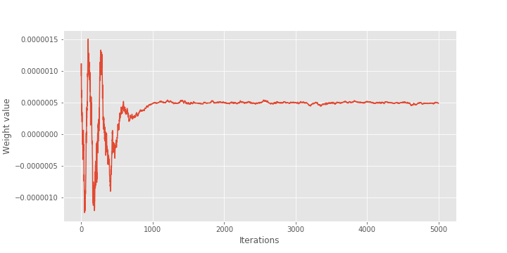
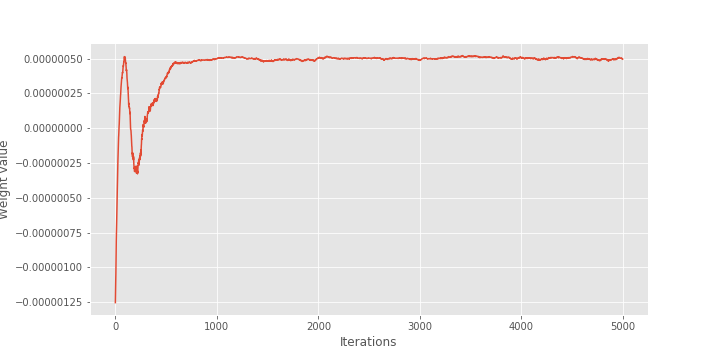
Figure 1: Lotka-Volterra example: first 5000 weights of the cube methods, based on full (top) or diagonal (bottom) set of covariates.

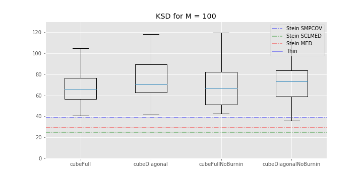
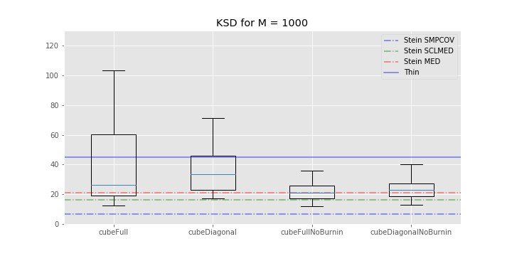
Figure 2: Lotka-Volterra example: box-plots of the kernel Stein discrepency for all the cube method variations, the KSD method for three kernels and the usual thinning method. Top: $M=100$. Bottom: $M=1000$. (In the top plot, standard thinning is omitted to improve clarity, as corresponding value is too high.)

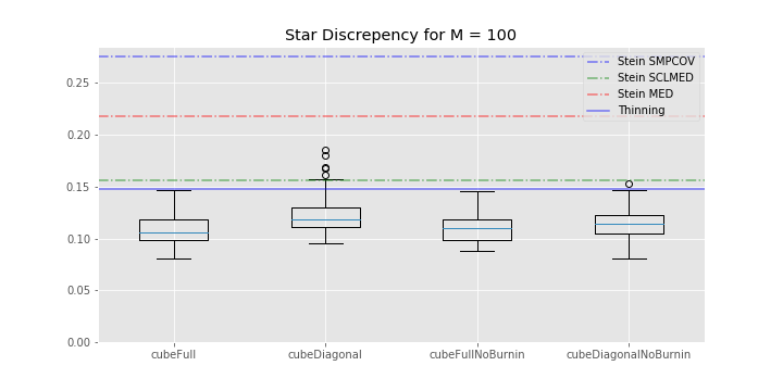
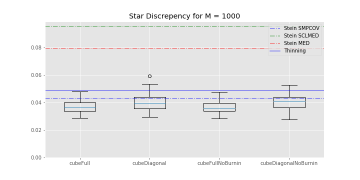
Figure 3: Lotka-Volterra example: box-plots of the star discrepency for all the cube method variations, the KSD method for three kernels and the usual thinning method. Top: $M=100$. Bottom: $M=1000$.

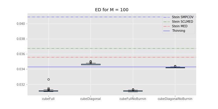
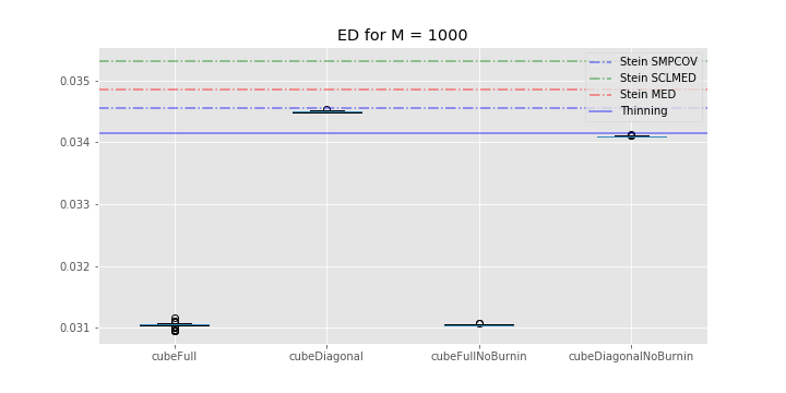
Figure 4: Lotka-Volterra example: boxplots of the energy distance for all the cube method variations, the KSD method for three kernels and the usual thinning method. Top: $M=100$. Bottom: $M=1000$.

First, we see that regarding the kernel Stein discrepancy metric, Figure 2, the KSD method performs better than the standard thinning procedure and the cube method. This is not surprising since even if this method does not properly minimizes the Kernel-Stein Discrepency, this is still its target. We also see that for $M=1000$, the KSD method performs a bit better than our cube method which in turn performs better than the standard thinning procedure. Note that the relative performance of the KSD method to our cube methods depends on the kernel that is being used and that there is no way to determine which kernel will perform best before running any experiment.

The picture is different for $M=100$: KSD thinning outperforms standard thinning, which in turn outperforms all of our cube thinning variations. Once again, the fact that the KSD method performs better than any other method seems reasonable: since it is about minimizing the Kernel-Stein Discrepancy, the KSD method is ”playing at home” on this metric.

If we look at Figure 4, we see that all of our cube methods outperform the KSD method with any kernel. Interestingly, the standard thinning methods has a similar Energy Distance as the cube methods with ”diagonal” control variates. These observations are true for both $M=100$ and $M=1000$. We can also note that the cube method with the full set of control variates tends to perform much better than its ”diagonal” counterpart, whatever the value of $M$.

Finally, looking at Figure 3, it is clear that the KSD method - with any kernel - performs worse than any cube method in terms of star discrepancy.

Overall, the relative performance of the cube methods and KSD methods can change a lot depending on the metric being used and the number of points we keep. In addition, while all the cube methods tend to perform roughly the same, this is not the case of the KSD method, whose performances depend on the kernel we use. Unfortunately, we have no way to determine beforehand which kernel will perform best. This is a problem since the KSD method is computationally expensive for subsamples of cardinal $M\gg 100$.

Thus, by and large, cube thinning seems much more convenient to use (both in terms of CPU time and sensitivity to tuning parameters) while offering, roughly, the same level of statistical performance.

5.3 Truncated Normal

In this example, we use the (random-scan version of) the Gibbs sampler of Robert and Casella, (2004) to sample from 10-dimensional multivariate normal truncated to $[0,\infty)^{10}$. We generated the parameters of this truncated normal as follows: the mean was set as the realization of a 10-dimensional standard normal distribution, while for the covariance matrix $\Sigma$ we first generated a matrix $M\in\mathcal{M}_{10,10}(\mathbb{R})$ for which each entry was the realization of a standard normal distribution. Then we set $\Sigma=M^{T}M$.

Since we are using a Gibbs sampler, we have access to the Gibbs control variates of Dellaportas and Kontoyiannis, (2011), based on the expectation of each update (which amounts to simulating from a univariate Gaussian). Thus, we consider 10 control variates.

The Gibbs sampler is run for $N=10^{5}$ iterations; no burn-in is performed. We compare the following estimators of the expectation of the target distribution the standard estimator, based on the whole chain (‘usualEstim’ in the plots), the estimator based on standard thinning (‘thinEstim’ in the plots), the control variate estimator based on the whole chain, i.e. (7) (’regressionEstim’ in the plots), and finally our cube estimator described in Section 4 (‘cubeEstim’ in the plots). For standard thinning and cube thinning, the thinning sample size is set to $M=100$, which corresponds to a compression factor of $10^{3}$.

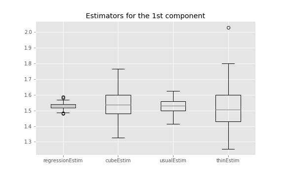
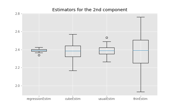
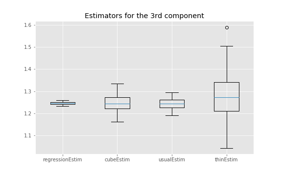
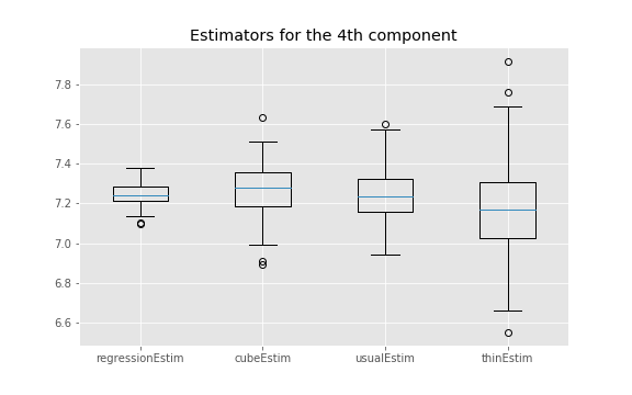
Figure 5: Truncated normal example: box-plots over 100 independent replicates of each estimator; see text for more details.

The results are shown in Figure 5. First, we can see that the control variates we chose lead to a substantial decrease in the variance of the estimates for regressionEstim compared to usualEstim. Second, the cube estimator performs worse than the regression estimator in terms of variance, but this was expected, as explained in Section 4. More interestingly, if we cannot say that the cube estimator performs better than the usual MCMC estimator in general, we can see that on some components it performs as good or even better, even though the cube estimator uses only $M=100$ points while the usual estimator uses $10^{5}$ points. This is largely due to the excellent choice of the control variates. Finally, the cube estimator outperforms the regular thinning estimator on every component, sometimes significantly.

Appendix A Details on the landing phase

The landing phase seeks to generate a random vector $S$ in $\{0,1\}^{N}$, with expectation $\pi^{\star}$ (the output of the flight phase), which minimises the criterion $\mbox{tr}(M\mathrm{Var}(\hat{V}|\pi^{\star}))$ for a certain matrix $M$. (The notation $\cdot|\pi^{\star}$ refers to the distribution of $S$ conditional on $\pi(t)=\pi^{\star}$ at the end of the flight phase.)

Since $\mathrm{Var}(S)=\mathrm{Var}(\mathbb{E}[S|\pi^{\star}])+\mathbb{E}[\mathrm{Var}(S|\pi^{\star})]$ by the law of total variance, and since the first term is zero (as $\mathbb{E}[S|\pi^{\star}]=\pi^{\star}$), we have

$$\mathrm{Var}(\hat{V})=\mathbb{E}[\mathrm{Var}(\hat{V}|\pi^{\star})]=\mathbb{E}[A\mathrm{Var}(S|\pi^{\star})A^{t}].$$ (21)

and thus:

$$\mbox{tr}(M\mathrm{Var}(\hat{V}|\pi^{\star}))=\sum_{s\in\{0,1\}^{N}}p(s|\pi^{\star})(s-\pi^{\star})^{t}A^{t}MA(s-\pi^{\star}).$$ (22)

Choosing $M=(AA^{t})^{-1}$, as recommended by Deville, (2004), amounts to minimising the distance to the hyperplane ‘on average’. Let $C(s)=(s-\pi^{\star})^{t}A^{t}(AA^{t})^{-1}A^{t}(s-\pi^{\star})$, then the minimisation program is equivalent to the following linear programming problem over $q$ variables only:

$$\min_{\xi^{\star}(.)}\sum_{s^{\star}\in\mathcal{S^{\star}}}C(s^{\star})\xi^{\star}(s^{\star})$$ (23)

with constraints $\sum_{s^{\star}\in\mathcal{S^{\star}}}\xi^{\star}(s^{\star})=1$, $0\leq\xi^{\star}(s^{\star})\leq 1$, $\sum_{s^{\star}\in\mathcal{S^{\star}}|s^{\star}_{k}=1}\xi^{\star}(s^{\star})=\pi^{\star}_{k}$ for every $k\in U^{\star}$ and $\mathcal{S^{\star}}=\{0,1\}^{q}$ where $q=\mathrm{card}(U^{\star})$ and $U^{\star}=\{k\in U:\,0<\pi^{\star}[k]<1\}$. Here $\xi^{\star}$ denotes the marginal distribution of the components $U^{\star}$ of the sampling design $\xi$ and $C(s^{\star})$ must be understood as $C(s)$ with the components of $s\notin U^{\star}$ being fixed by the result of flight phase, thus in this minimization problem $C$ is in fact depending on the components of $s$ that are in $U^{\star}$ only.

The constraints define a bounded polyhedron. By the fundamental theorem of linear programming, this optimization problem has at least one solution on a minimal support, see Deville, (2004).

The flight phase ends on a vertex of $\mathcal{K}$ and, by Proposition 1 in Deville, (2004), $q\leq J$; typically $J\ll N$. This means that we are solving a linear programming problem in a dimension $q$ potentially much lower than the population size $N$, and if we do not have too many auxiliary variables, this optimization problem will not be computationally too expensive. In practice, a simplex algorithm is used to find the solution.

Appendix B Estimation of the energy distance

There are two difficulties with computing (20). First, it involves intractable expectations. Second, as pointed out at the end of Section 4.3, the empirical distribution generated by cube thinning, (19), is actually a signed measure.

Regarding the first issue, we can approximate (20) from our MCMC sample $X_{1},\dots,X_{N}$. That is, if our subsampled empirical measure writes $\hat{\nu}=\sum_{m=1}^{M}w_{m}\delta_{Z_{m}}$ and that we approximate the distribution associated with $p$ by $\hat{P}=(N-b)^{-1}\sum_{n=b+1}^{N}\delta_{X_{n}}$ where $1\leq b\leq N$ is the burn-in of the chain, then, we can estimate $ED(\hat{\mu},p)$ with $ED(\hat{\mu},\hat{P})$.

Regarding the second issue, we can generalize the energy distance to finite measures: suppose we have two finite and potentially signed measures $\nu_{1}$ and $\nu_{2}$, both defined on the same measurable space $(\Omega,\mathcal{P}(\Omega)\}$ where $\Omega=\{X_{1},\dots,X_{N}\}$ and $\mathcal{P}(\Omega)$ denotes the set of parts of $\Omega$. Suppose in addition that $\nu_{1}(\Omega)=\alpha_{1}$ and $\nu_{2}(\Omega)=\alpha_{2}$ with $\alpha_{1}\neq 0$ and $\alpha_{2}\neq 0$. We define the generalized energy distance as:

$$ED^{\star}(\nu_{1},\nu_{2})= \dfrac{2}{\alpha_{1}\alpha_{2}}\int_{\Omega}||x-y||_{2}d\nu_{1}(x)d\nu_{2}(y)$$

$$-\dfrac{1}{\alpha_{1}^{2}}\int_{\Omega}||x-x^{\prime}||_{2}d\nu_{1}(x)d\nu_{1}(x^{\prime})$$

$$-\dfrac{1}{\alpha_{2}^{2}}\int_{\Omega}||y-y^{\prime}||_{2}d\nu_{2}(y)d\nu_{2}(y^{\prime}).$$

Then, by negative definiteness of the application $\phi(x,y)=||x-y||_{2}$ on $\mathbb{R}^{N}\times\mathbb{R}^{N}$, we have that $ED^{\star}(\nu_{1},\nu_{2})\geq 0$ with equality if and only if $\dfrac{1}{\alpha_{1}}\nu_{1}=\dfrac{1}{\alpha_{2}}\nu_{2}$. Which means that the generalized energy distance is zero if and only if the two measures are equal up to a non-zero multiplicative constant, see Székely and Rizzo, (2005) for a demonstration. This generalized energy distance is also symmetric, but the triangle inequality does not hold. It is a pseudo-distance.

Thus we will use the following criterion, which we will abusively call the energy distance in the rest of the paper:

$${ED}^{\star}(\hat{\nu},\hat{P})= \dfrac{2}{(N-b)\alpha_{1}}\sum_{k=1}^{N}\sum_{n=b+1}^{N}\dfrac{\Omega}{M}sgn(w_{k})||X_{k}-X_{n}||_{2}\mathbf{1}_{\{S_{k}=1\}}$$

$$-\dfrac{1}{\alpha_{1}^{2}}\sum_{n=1}^{N}\sum_{k=1}^{N}\left(\dfrac{\Omega}{M}\right)^{2}sgn(w_{n})sgn(w_{k})||Z_{k}-Z_{n}||_{2}\mathbf{1}_{\{S_{k}=1\}}\mathbf{1}_{\{S_{n}=1\}}$$

where $\hat{\nu}$ is defined in (19) and we dropped the last term because it does not depend on $\hat{\nu}$ and it is a potentially expensive sum of $(N-b)^{2}$ terms.

Note that the probability of $\hat{\nu}(\Omega)$ being zero is non-null and then there is a non-negligible probability of ${ED}^{\star}(\hat{\nu},\hat{P})$ being undefined. However, this event is unlikely to happen.

References

- Brooks and Gelman, (1998) Brooks, S. and Gelman, A. (1998). Some issues for monitoring convergence of iterative simulations. Computing Science and Statistics, pages 30–36.
- Brosse et al., (2019) Brosse, N., Durmus, A., Meyn, S., Moulines, E., and Radhakrishnan, A. (2019). Diffusion approximations and control variates for MCMC. arXiv 1808.01665.
- Chauvet and Tillé, (2006) Chauvet, G. and Tillé, Y. (2006). A fast algorithm for balanced sampling. Computational Statistics, 21(1):53–62.
- Cowles and Carlin, (1996) Cowles, M. K. and Carlin, B. P. (1996). Markov chain Monte Carlo convergence diagnostics: a comparative review. J. Amer. Statist. Assoc., 91(434):883–904.
- Dellaportas and Kontoyiannis, (2011) Dellaportas, P. and Kontoyiannis, I. (2011). Control variates for estimation based on reversible Markov chain Monte Carlo samplers. Journal of the Royal Statistical Society: Series B (Statistical Methodology), 74(1):133–161.
- Deville, (2004) Deville, J.-C. (2004). Efficient balanced sampling: The cube method. Biometrika, 91(4):893–912.
- Geyer, (1992) Geyer, C. J. (1992). Practical Markov chain Monte Carlo. Statistical Science, 7(4).
- Glasserman, (2004) Glasserman, P. (2004). Monte Carlo methods in financial engineering, volume 53 of Applications of Mathematics (New York). Springer-Verlag, New York. Stochastic Modelling and Applied Probability.
- Hammer and Tjelmeland, (2008) Hammer, H. and Tjelmeland, H. (2008). Control variates for the Metropolis–Hastings algorithm. Scandinavian Journal of Statistics, 35(3):400–414.
- Klebanov, (2006) Klebanov, L. B. (2006). N-distances and Their Applications. The Karolinum Press, Charles University.
- Mak and Joseph, (2018) Mak, S. and Joseph, V. R. (2018). Support points. The Annals of Statistics, 46(6A).
- Mira et al., (2013) Mira, A., Solgi, R., and Imparato, D. (2013). Zero variance Markov chain Monte Carlo for Bayesian estimators. Stat. Comput., 23(5):653–662.
- Oates et al., (2016) Oates, C. J., Girolami, M., and Chopin, N. (2016). Control functionals for Monte Carlo integration. Journal of the Royal Statistical Society: Series B (Statistical Methodology), 79(3):695–718.
- Owen, (2013) Owen, A. B. (2013). Monte Carlo theory, methods and examples. Work in progress, available on the author’s web-site.
- Riabiz et al., (2020) Riabiz, M., Chen, W., Cockayne, J., Swietach, P., Niederer, S. A., Mackey, L., and Oates, C. J. (2020). Optimal thinning of MCMC output. arXiv 2005.03952.
- Robert and Casella, (2004) Robert, C. P. and Casella, G. (2004). Monte Carlo Statistical Methods. Springer New York.
- Székely and Rizzo, (2005) Székely, G. J. and Rizzo, M. L. (2005). A new test for multivariate normality. Journal of Multivariate Analysis, 93(1):58–80.