Characterization of topological phase transitions from a non-Abelian topological state and its Galois conjugate through condensation and confinement order parameters

Abstract

Topological phases exhibit unconventional order that cannot be detected by any local order parameter. In the framework of Projected Entangled Pair States (PEPS), topological order is characterized by an entanglement symmetry of the local tensor that describes the model. This symmetry can take the form of a tensor product of group representations (for quantum double models $D(G)$ of a group $G$), or in the more general case a correlated symmetry action in the form of a Matrix Product Operator (MPO), that encompasses all string-net models, including those which are not quantum double models. Among other things, these entanglement symmetries allow for the succinct description of ground states and topological excitations (anyons). Recently, the idea has been put forward to use those symmetries and the anyonic objects they describe as order parameters for probing topological phase transitions, and the applicability of this idea has been demonstrated for Abelian groups. In this paper, we extend this construction to the domain of non-Abelian models with MPO symmetries, and we use it to study the breakdown of topological order in the double Fibonacci (DFib) string-net model and its Galois conjugate, namely the non-hermitian double Yang-Lee (DYL) string-net model. We start by showing how to construct topological order parameters for condensation and deconfinement of anyons using the MPO symmetries. Subsequently, we set up interpolations from the DFib and the DYL model to the trivial phase, and we show that these can be mapped to certain restricted solid on solid (RSOS) models, which are equivalent to the $((5\pm\sqrt{5})/2)$-state Potts model, respectively. Moreover, the order parameter for condensation maps to the RSOS order parameter. The known exact solutions of the statistical models subsequently allow us to locate the critical points of the models, and to predict the critical exponents for the order parameters from conformal filed theory. We complement this by numerical study of the phase transitions, which fully confirms our theoretical predictions; remarkably, we find that both models exhibit a duality between the behavior of order parameters for condensation and deconfinement.

I Introduction

Landau’s theory of spontaneous symmetry breaking is one of the cornerstones of condensed matter physics. It captures the nature of phases and phase transitions via local order parameters characterizing the spontaneous breaking of the global symmetries of the system. This has been challenged by the discovery of topologically ordered phases, which are non-trivial phases without any global symmetries, and which therefore cannot be characterized by local order parameters [1]. A prototypical example of a topological phase is realized by the toric code model, and its generalizations based on quantum doubles $D(G)$ of a finite group $G$ [2]. Although there is no global symmetry, those models can be mapped to lattice gauge theories with symmetry group $G$. In addition to those phases, there exist a large class of more exotic topological phases where anyons carry degrees of freedom with irrational dimensions and whose gauge symmetry cannot be described by group theory. The concept of topological phases has even been extended to non-hermitian systems [3], which exhibit new kinds of topological orders that cannot exist in hermitian systems.

The fixed point wavefunctions of non-chiral topological phases can be realized by so-called string-net models supporting anyonic excitations [4]. Both ground states of string-nets and excited states carrying anyonic quasiparticles can be represented by projected entangled pair states (PEPS)[5, 6], which provide a description of the global wavefunction as a tensor network built from local tensors. Here, the topological order is accompanied by the presence of certain group or Matrix Product Operator (MPO) symmetries in the entanglement degrees of freedom of the tensor, which can be used to parametrize the ground space manifold and anyonic excitations alike [7, 8, 9]. The description of topologically ordered systems as PEPS based on entanglement symmetries suggests a natural way to construct and study topological phase transitions within PEPS, by applying deformations to the physical degrees of freedom that drive the system to a different phase (such as a trivial product state) [10, 11, 12, 13, 14, 15, 16, 17]. In this language, the entanglement symmetry in the tensor is preserved throughout the path, but at some point, it no longer manifests itself in topological order.

From the point of view of an effective theory, topological phase transitions can be understood through the process of anyon condensation and confinement: At a transition from a topological phase to one with a lesser degree of topological order (such as a trivial phase), some anyons condense into the ground state, and as a consequence, anyons that braid non-trivially with condensed anyons must confine [18, 19]. If the wavefunction of the system is given as a PEPS with entanglement symmetries, such as for the interpolating families referenced above, this process can be probed through topological order parameters which are constructed at the entanglement level, and which probe the condensation and deconfinement of anyons; notably, those order parameters can be used to extract critical exponents which characterize the universal nature of the phase transition, despite the lack of local order parameters [20, 13, 21]. However, up to now, the construction of condensation and deconfinement order parameters, and the extraction of their universal scaling behavior at criticality, has only been carried out for Abelian symmetry groups.

In this paper, we construct topological order parameters and extract the critical exponents at the phase transitions for some of the most important non-Abelian topological models, which furthermore cannot be constructed as the quantum double of a group: The double Fibonacci (DFib) string-net model [4, 22, 23, 24, 25], and its Galois conjugate, the double Yang-Lee (DYL) string-net model, which comes with a non-hermitian parent Hamiltonian [3, 26, 27]. For both models, we set up a deformation that smoothly changes the model towards a trivial product state, driving it through a topological phase transition. We show how to construct order parameters for condensation and deconfinement, using the MPOs underlying the entanglement symmetry of the tensors. We continue by showing that the normalization of our deformed PEPS wavefunctions can be mapped to the partition function of a restricted solid on solid (RSOS) model associated with the Dynkin diagram $D_{6}$, where the order parameter for condensation maps to the corresponding order parameter of the RSOS model. That RSOS model, in turn, is known to map to the $q$-state Potts model with $q=(2+\phi)$ and $q=(2-1/\phi)$ for the DFib and the DYL model, respectively (where $\phi=(1+\sqrt{5})/2$); for the DFib model, a duality to the same $q$ Potts model, albeit on the triangular lattice, has also been shown directly for alternative deformations [28, 29]. This duality mapping allows us both to locate the exact critical point, and to predict the critical exponents for the order parameter (i.e., condensation); the self-duality of the model then suggests the same critical exponents for the disorder parameters.

We supplement our analytical arguments with numerical study, which fully matches the analytical findings, and in particular confirms the point that the critical exponents for the disorder parameter (the anyon deconfinement fraction) are the same as those for the order parameter (the anyon condensate fraction), reinforcing the role played by the self-duality of the Potts model. Specifically, for the DFib model, we obtain that it is described by the unitary minimal model with $c=14/15$, with critical exponents $\eta=4/15$, $\nu=3/4$, and $\beta=1/10$, with $c$ the central charge and $\eta$, $\nu$, and $\beta$ the exponents for correlations at criticality, correlation length, and order parameter, respectively. The DYL model is described by a non-unitary minimal model with $c=8/35$, where the critical exponents are $\eta=8/35$, $\nu=7/6$, and $\beta=2/15$.

The paper is organized as follows. Section II reviews the PEPS description of the ground states and excited states of the string-net models. Section III focuses on the analytic and numerical results of DFib string-net, and Sec. IV focuses on the analytic and numerical results of the DYL string-net. Finally, we conclude in Sec. V.

II PEPS representation for the string-net wavefunctions

II.1 String-net models with only one kind of strings

A string-net model [4] is specified by a set of data $\{d_{i},N_{ij}^{k},F_{tsu}^{ijk}\}$, where the indices can take values in a set $\mathcal{A}$ of “particles”, including the “identity particle” $1\in\mathcal{A}$. Here, the fusion rule $N_{ij}^{k}\in\mathbb{N}$ counts the possible ways in which the particles $i$ and $j$ can fuse to $k$, $d_{i}$ is the quantum dimension of $i$, and the $F_{tsu}^{ijk}$ must satisfy the so-called pentagon equations [4]. In this work, we are concerned with models with $\mathcal{A}=\{1,\tau\}$, which possess a non-trivial fusion rule

$${1}\times{1}={1},\quad{1}\times{\tau}={\tau}\times{1}={\tau},\quad{\tau}\times{\tau}={1}+{\tau}\ .$$ (1)

This fusion rule allows for two solutions of the pentagon equations [4]: one unitary solution: the doubled Fibonacci (DFib) string-net model, and one non-unitary solution: the doubled Yang-Lee (DYL) string-net model, which is the Galois conjugate of the DFib string-net model [3]. For the DFib theory, $d_{1}=1$ and $d_{\tau}=\phi=(1+\sqrt{5})/2$, and

$$F^{\tau\tau i}_{\tau\tau j}=\frac{1}{\phi}\left(\begin{array}[]{cc}1&\sqrt{\phi}\\ \sqrt{\phi}&-1\\ \end{array}\right)_{ij}\ ,$$ (2)

while all other entries allowed by the fusion rule $N_{ij}^{k}$ are $1$, and $0$ otherwise. The corresponding data for the DYL theory are obtained by replacing $\phi$ with $\phi^{\prime}=-1/\phi=(1-\sqrt{5})/2$, resulting in $d_{1}=1$, $d_{\tau}=\phi^{\prime}$ and the non-trivial entries of the $F$ symbol being

$$F^{\tau\tau i}_{\tau\tau j}=\frac{1}{\phi^{\prime}}\left(\begin{array}[]{cc}1&\sqrt{\phi^{\prime}}\\ \sqrt{\phi^{\prime}}&-1\\ \end{array}\right)_{ij}.$$ (3)

The string-net model wavefunction on the honeycomb lattice is obtained by assigning a degree of freedom $\{\lvert 0\rangle,\lvert\tau\rangle\}$ to each vertex, and constructing the wavefunction as a superposition of all configurations that satisfy the fusion rule $N_{ij}^{k}$ across every vertex, with amplitudes constructed from the quantum dimension $d_{i}$ and the $F$ symbol [4]. These wavefunctions are exact ground states of a local Hamiltonian which can also be constructed from the data $\{d_{i},N_{ij}^{k},F_{tsu}^{ijk}\}$ [4]. An important difference between the Hamiltonians of DFib and DYL string-net models is that the former is hermitian, while the latter is non-hermitian; yet, the Hamiltonian of the DYL string-net model has an entirely real energy spectrum [3]. The model is topologically ordered and possesses anyonic excitations, which can be constructed from the underlying particles $\mathcal{A}$ through doubling (by coupling a chiral and an anti-chiral copy with particle content $\mathcal{A}$), and which we will denote by $\{\bm{1},\bm{\tau},\bm{\bar{\tau}},\bm{b}\}$, where $\bm{\tau}$ and $\bm{\bar{\tau}}$ inherit the fusion rule (1), and $\bm{b}=(\tau,\bar{\tau})$ is the boson.

II.2 PEPS representation for the ground states

The construction of Projected Entangled Pair States (PEPS) is illustrated in Fig. 1(a): Here, each ball denotes a tensor, and the legs denote indices. Connecting legs amounts to contracting (i.e., identifying and summing) the index. Legs perpendicular to the $xy$ plane are physical indices and legs parallel the $xy$ plane are the virtual indices. Arranging local tensors in a two-dimensional grid as shown in the figure (possibly on a different lattice) and contracting their virtual indices give rise to the PEPS. The ground state wavefunction of string-net models can be explicitly expressed as a PEPS [5, 6], whose local tensors can be constructed from $d_{i}$ and $F^{ijk}_{tsu}$. We describe this construction in detail in Appendix A. In the PEPS framework, the topological order is characterized by virtual symmetries of the tensors described by matrix product operators (MPOs) [7, 9, 8]. For the DFib or DYL string-net model, there are two different MPOs describing their order: One is the trivial MPO $O_{1}\equiv\openone$, and the other is the non-trivial MPO $O_{\tau}$. Again, their definitions are presented in Appendix A. The defining feature of these MPOs is that they can be freely moved. Thus, inserting the non-trivial MPO $O_{\tau}$ into the virtual level of the PEPS, as shown in Fig. 1(b), results in another topologically degenerate ground state. Notice that since $O_{1}$ equals the identity, a PEPS with $O_{1}$ inserted is the same state as the one without inserting any MPO.

On a torus, the ground space of the DFib or DYL string-net model has a four-fold topological degeneracy. A canonical basis of the ground state subspace is given by the minimally entangled states (MESs) $|\bm{\alpha}\rangle$, which have well defined anyonic flux $\bm{\alpha}$ along one direction of the torus [30], where $\bm{\alpha}=\bm{1},\bm{\tau},\bm{\bar{\tau}}$ and $\bm{b}$. As shown in Fig. 1(c), in order to obtain an MES with a well-defined horizontal anyonic flux, one needs to insert a vertical idempotent into the PEPS [31]. The idempotents come from the tube algebra [32, 9], and consist of the MPO tensors together with specific tensors inserted at the crossing point, see Appendix A for their definitions. There are four central idempotents $P_{\bm{1}},P_{\bm{\tau}},P_{\bm{\bar{\tau}}}$ and $P_{\bm{b}}$ of the tube algebra. By further specifying the type of the horizontal MPO $O_{n}$ in Fig. 1(c) using a second (non-boldface) subscript, it can be found that the first three central idempotents are one dimensional: $P_{\bm{1}}=P_{\bm{1}1},P_{\bm{\tau}}=P_{\bm{\tau}\tau},P_{\bm{\bar{\tau}}}=P_{\bm{\bar{\tau}}\tau}$, but the last central idempotent is two dimensional: $P_{\bm{b}}=P_{\bm{b}1}\oplus P_{\bm{b}\tau}$; see Appendix A for details. Starting from the PEPS in Fig. 1(a), we obtain the MESs $|\bm{1}\rangle$ and $|\bm{b}\rangle$ by inserting either the idempotent $P_{\bm{1}}$ or $P_{\bm{b}1}$ in the vertical direction; and starting from the PEPS in Fig. 1(b), we obtain the MESs $|\bm{b}\rangle$, $|\bm{\tau}\rangle$, or $|\bm{\bar{\tau}}\rangle$ by inserting either the idempotent $P_{\bm{b}\tau}$, $P_{\bm{\tau}}$, or $P_{\bm{\bar{\tau}}}$ in the vertical direction.

Figure 1: (a) A ground state of one of the topological models represented by a PEPS; in the box is the local tensor generating the PEPS. (b) A PEPS with the non-trivial MPO $O_{\tau}$ inserted yields another ground state; in the box is the local tensor generating the MPO. (c) The MES $|\bm{\alpha}\rangle$ with a well-defined horizontal anyonic flux $\bm{\alpha}$ obtained by inserting the vertical idempotent $P_{\bm{\alpha}n}$ into the PEPS in (a) or (b), where $n=1,\tau$ denotes the type of the horizontal MPO. (d) An excited state carrying an anyon $\bm{\alpha}$; the green triangle is the rank-3 endpoint tensor $E_{\bm{\alpha}n}$.

II.3 PEPS representation for the excited states

The PEPS can also be used to represent the excited states of the string-net models. In order to describe the complete anyonic excitations, the extended string-net models have been proposed [33]. A plaquette term of an extended string-net model is the trivial central idempotent of the tube algebra and the anyonic excitations are projected out by other non-trivial central idempotents acting around the plaquette. When applied in the PEPS framework, an anyon excition is represented by a rank three end point tensor $E_{\bm{\alpha}n}$ with an MPO string attached to it [34], where the first subscript $\bm{\alpha}=\bm{1},\bm{b},\bm{\tau},\bm{\bar{\tau}}$ denotes the anyon type, and the second subscript $n=1,\tau$ denotes the type of attached MPO string, see Fig. 1(d). The end tensor $E_{\bm{\alpha}n}\equiv E_{\bm{\alpha}n}(d_{i},F_{tsu}^{ijk},R_{k}^{ij})$ is determined by $d_{i}$ and $F_{tsu}^{ijk}$ together with a tensor $R_{k}^{ij}$, which characterizes the braiding statistics of $i$ and $j$ particles subjected to their fusion channel $k$, see Appendix A. According to the definition of $E_{\bm{\alpha}n}$, there are five such end tensors: $E_{\bm{1}1}$, $E_{\bm{\tau}\tau}$, $E_{\bm{\bar{\tau}}\tau}$, $E_{\bm{b}1}$ and $E_{\bm{b}\tau}$, indicating that only trivial (non-trivial) MPO strings can be attached to $\bm{1}$ ($\bm{\tau}$ and $\bm{\bar{\tau}}$) excitations, while both trivial and non-trivial MPO strings can be attached to the $\bm{b}$ excitations. Since the tensor $E_{\bm{b}1}$ has the trivial MPO $O_{1}$ attached to it, this means that the $\bm{b}$ excitation can be described by locally modifying the PEPS on the virtual level, with no MPO string attached.

III DFib string-net

III.1 Deformed DFib string-net wavefunction

Let us now investigate what happens when we drive the DFib string-net model into the trivial phase. To this end, we study a deformation of the DFib string-net wavefunction, obtained by imposing a string tension on the $\tau$ string (driving the system towards the topologically trivial vacuum state). Specifically, we add different tensions $K_{1}$, $K_{2}$, and $K_{3}$ to the inequivalent edges of the honeycomb lattice,

$$|\Psi(K_{1},K_{2},K_{3})\rangle=\prod_{i_{1},i_{2},i_{3}}e^{\frac{K_{1}\sigma^{z}_{i_{1}}+K_{2}\sigma^{z}_{i_{2}}+K_{3}\sigma^{z}_{i_{3}}}{4}}|\Psi_{\text{DFib}}\rangle,$$ (4)

where $\sigma^{z}|1\rangle=|1\rangle$, $\sigma^{z}|\tau\rangle=-|\tau\rangle$, and $\{i_{1}\},\{i_{2}\}$, $\{i_{3}\}$ denote the edges in each of the three directions; see Fig. 2(a). Importantly, since the deformation acts on the physical degrees of freedom, the virtual MPO symmetry of the PEPS is preserved, allowing us to construct the topological sectors and anyonic excitations on top of the PEPS $|\Psi(K_{1},K_{2},K_{3})\rangle$ as before.

In addition, the deformed wave function still has a frustration-free parent Hamiltonian, which can be constructed by conjugating the Hamiltonian of the DFib model (with the ground state energy of each term shifted to zero) with the inverse of local deformation [35, 36]. Specifically, the Hamiltonian $H=\sum_{r}h_{r}$ of the DFib string-net is a sum of the local positive semi-definite projectors $h_{r}$ acting on the region $r$, and the deformation matrix $\exp(K_{t}\sigma^{z}_{i_{t}}/4)$ with $t=1,2,3$ is also a local positive definite operator, so that the parent Hamiltonian of the deformed wave function is

$$H(K)=\sum_{r}P_{r}^{-1}h_{r}P_{r}^{-1}\ ,$$ (5)

where $P_{r}=\prod_{i_{t}\in r}\exp(K_{t}\sigma^{z}_{i_{t}}/4)$. The possible quantum critical points of this Rokhsar-Kivelson type Hamiltonian are the so-called conformal quantum critical points [37], where all equal-time correlation functions are described by two-dimensional conformal field theories (CFTs), which can be extracted from the transfer operators of the wavefunction norms at the critical points.

When $K_{1}=K_{2}=K_{3}=K$, it has been shown that the norm of the deformed wavefunction can be mapped to the partition function of the isotropic $(\phi+2)$-state Potts model on the dual triangular lattice[28, 29]. As the string-tension $K$ increases, there is a phase transition from the topological phase to the non-topological phase, where the position of the critical point and the CFT describing it are known from the exact solution of the Potts model.

We will in the following consider a different case, namely $K_{1}=K_{2}=K$, $K_{3}=0$. As we prove in Appendix B by also taking the virtual degrees of freedom in the PEPS into account, the norm of the deformed PEPS equals the partition function of an RSOS model on the square lattice associated with the $D_{6}$ Dynkin diagram[38]. Moreover, it has been shown that the partition functions of RSOS models associated with $D$ type Dynkin diagrams and the partition functions of Potts models are equivalent[39]. Therefore, we can conclude that the norm of the deformed wavefunction maps to the partition function of the $q=(\phi+2)$-state Potts model on the square lattice:

$$\langle\Psi(K,K,0)|\Psi(K,K,0)\rangle\propto\mathcal{Z}(q=\phi+2,K)\ .$$ (6)

If we think of the virtual degrees of freedom of the PEPS as the “Potts spins” and the physical degrees of freedom as their “domain walls” – a picture which e.g. underlies the well-known mapping between $\mathbb{Z}_{N}$ quantum doubles and Potts or clock models with $q=N$ – we see that the disordered phase of the Potts model corresponds to the topological phase at small $K$ (where domain walls strongly fluctuate), while the ordered phase of the Potts model corresponds to the trivial phase at large $K$ (where domain wall fluctuations are supressed).

Under the self-duality of the the square lattice Potts models, the partition function $\mathcal{Z}(q,K)$ of the $q$-state Potts model is mapped to $\mathcal{Z}(q,K^{\star})$, where $K$ and $K^{\star}$ satisfy $(e^{K}-1)(e^{K^{\star}}-1)=q$ [40]. The critical point of the $q$-state Potts model (for $q\leq 4$, as is the case here) is known to be located at the self-dual point. Its position $e^{K_{c}}$ and the central charge $c$ of the CFT describing it are [41]

$$e^{K_{c}}=1+\sqrt{q}\ ,\quad c=1-6/[\delta(\delta-1)]\ ,$$ (7)

where $q=4\cos^{2}(\pi/\delta)$. When $q=\phi+2$, $e^{K_{c}}\approx 2.9021$, and the CFT describing the critical point is the unitary minimal model with the central charge $c=14/15$.

Figure 2: (a) The physical degrees of freedom of the model (open circles) are located on the edges of a honeycomb lattice. The edges are classified into three sets $\{i_{1}\}$, $\{i_{2}\}$, and $\{i_{3}\}$, according to their directions. (b) The transfer operators $\mathbb{T}_{1}^{1}$ and $\mathbb{T}_{\tau}^{\tau}$, where the superscripts (subscripts) represent the types of MPO tensors inserted in bra (ket) layers. (c) The numerator of the condensate fraction $\mathcal{C}_{\bm{b}}^{\bm{1}}$ represented as a tensor network. (d) The numerator of the deconfinement fraction $\mathcal{C}_{\bm{\tau}}^{\bm{\tau}}$ represented as a tensor network.

III.2 Condensate and deconfinement fractions and correlation functions

Topological phase transitions in PEPS can be characterized by order parameters constructed from the anyonic excitations of the theory, which measure the condensation and deconfinement of the anyons, respectively [20, 13]. Only anyons with bosonic self-statistics can condense [18, 19]; for the DFib model, this is only the $\bm{b}$ anyon. We define its condensate fraction as

$$\mathcal{F}_{\bm{b}}^{\bm{1}}=\frac{\langle\bm{1}|\dot{\bm{b}}_{i}\rangle}{\langle\bm{1}|\bm{1}\rangle}\ ,$$ (8)

where $|\bm{1}\rangle$ is the minimally entangled ground state with a trivial anyon flux, and $|\dot{\bm{b}}_{i}\rangle$ is an excited state obtained by creating a $\bm{b}$ anyon at position $i$ on top of $|\bm{1}\rangle$. Since the $\bm{b}$ anyons created using $E_{\bm{b}1}$ and $E_{\bm{b}\tau}$ are equivalent, we choose to create the $\bm{b}$ anyon using $E_{\bm{b}1}$ for simplicity, since this does not require to attach an MPO string on the virtual level of PEPS, see Fig. 2(c). In the topological phase, $|\dot{\bm{b}}_{i}\rangle$ is a well defined excited state which is orthogonal to the ground state $|\bm{1}\rangle$, and thus, we expect that the condensate fraction is zero. In the topologically trivial phase, which is obtained by condensing the $\bm{b}$ anyon, we correspondingly expect a non-zero condensate fraction.

In the topologically trivial phase, the condensation of $\bm{b}$ must be accompanied by the confinement of the $\bm{\tau}$ and $\bm{\bar{\tau}}$ anyons, because they have non-trivial mutual statistics with $\bm{b}$ [18, 19]. The deconfinement fraction of $\bm{\tau}$ can be defined as

$$\mathcal{F}_{\bm{\tau}}^{\bm{\tau}}=\frac{\langle\dot{\bm{\tau}}_{i}|\dot{\bm{\tau}}_{i}\rangle}{\langle\bm{1}|\bm{1}\rangle}\ ,$$ (9)

where $|\dot{\bm{\tau}}_{i}\rangle$ is obtained by inserting an end tensor $E_{\bm{\tau}}$ with a semi-infinite non-trivial MPO string attached, see Fig. 2(d). Because $\bm{\tau}$ anyons are deconfined (confined) in the topological (non-topological) phase, we expect the deconfinement fraction to be nonzero (zero).

These anyonic order parameters for topological phases also open up a new perspective on order and disorder parameters for the corresponding Potts model with non-integer $q$: As we discussed before, the topological and trivial phases of the deformed DFib PEPS are mapped to the disordered and ordered phases of the (non-integer) $q=(\phi+2)$-state Potts model. Thus, we can interpret the condensate fraction $\mathcal{F}_{\bm{b}}^{\bm{1}}$ as an order parameter for the Potts model, since it is non-zero (zero) in the ordered (disordered) phase. On the other hand, the deconfinement fraction $\mathcal{F}_{\bm{\tau}}^{\bm{\tau}}$ can be interpreted as a disorder parameter [42] for the $q=(\phi+2)$-state Potts model, since it is non-zero (zero) in the disordered (ordered) phase. For the ordered phase, we strengthen this connection by proving in Appendix B that the condensate fractions $\mathcal{F}_{\bm{b}}^{\bm{1}}$ and $\mathcal{F}_{\bm{1}}^{\bm{b}}$ are equivalent to the expectation values of the local order parameters of the RSOS model[43]. Together with the mapping between RSOS and Potts models, this further strengthens the interpretation of the condensate fraction as an order parameter for the Potts model.

In addition to the condensate and deconfinement fractions, the correlation functions between pairs of anyons also contain useful information; in fact, the order parameters above can (just as any order parameter) be seen as the square root of the asymptotic value of an underlying correlation function. Specifically, the correlation function underlying the condensate fraction of $\bm{b}$ anyons can be defined by creating a pair of $\bm{b}$ anyons in the ket layer and computing their overlap with the trivial MES, ${\langle\bm{1}|\dot{\bm{b}}_{i}\dot{\bm{b}}_{j}\rangle}/{\langle\bm{1}|\bm{1}\rangle}$. Specifically, in the topological phase, it will display an exponential decay

$$\mathcal{C}_{\bm{b}}^{\bm{1}}(|i-j|)=\frac{\langle\bm{1}|\dot{\bm{b}}_{i}\dot{\bm{b}}_{j}\rangle}{\langle\bm{1}|\bm{1}\rangle}\propto\exp{\left(-\frac{|i-j|}{\xi^{\bm{1}}_{\bm{b}}}\right)}\ ,$$ (10)

where the inverse correlation length $1/\xi^{\bm{1}}_{\bm{b}}$ can be interpreted as the “anyon mass gap” [21], while in the trivial phase, it will converge to $\mathcal{|}F^{\bm{1}}_{\bm{b}}|^{2}>0$. Similarly, the correlation function underlying the confinement of $\bm{\tau}$ can be constructed by creating a pair of $\bm{\tau}$ anyons and considering their norm, ${\langle\dot{\bm{\tau}}_{i}\dot{\bm{\tau}}_{j}|\dot{\bm{\tau}}_{i}\dot{\bm{\tau}}_{j}\rangle}/{\langle\bm{1}|\bm{1}\rangle}$, which we expect to decay exponentially in the topologically trivial phase,

$$\mathcal{C}_{\bm{\tau}}^{\bm{\tau}}(|i-j|)=\frac{\langle\dot{\bm{\tau}}_{i}\dot{\bm{\tau}}_{j}|\dot{\bm{\tau}}_{i}\dot{\bm{\tau}}_{j}\rangle}{\langle\bm{1}|\bm{1}\rangle}\propto\exp{\left(-\frac{|i-j|}{\xi_{\bm{\tau}}^{\bm{\tau}}}\right)},$$ (11)

with $\xi_{\bm{\tau}}^{\bm{\tau}}$ the confinement length scale; again, in the topological phase, this will converge to $|\mathcal{F}_{\bm{\tau}}^{\bm{\tau}}|^{2}$. Again, both of these correlation lengths can also be interpreted in the Potts model as the correlation lengths corresponding to the order and disorder parameter, respectively.

Finally, let us define a trivial correlation function

$$\mathcal{C}_{\bm{1}}^{\bm{1}}(|i-j|)=\frac{\langle\bm{1}|\sigma_{i}^{z}\sigma_{j}^{z}|\bm{1}\rangle}{\langle\bm{1}|\bm{1}\rangle}-\frac{\langle\bm{1}|\sigma_{i}^{z}|\bm{1}\rangle}{\langle\bm{1}|\bm{1}\rangle}\frac{\langle\bm{1}|\sigma_{j}^{z}|\bm{1}\rangle}{\langle\bm{1}|\bm{1}\rangle},$$ (12)

where the operators $\sigma_{i}^{z}$ act on the physical level of the PEPS instead of on the virtual level. Since the internal energy of the Potts model is $-\frac{1}{\mathcal{Z}}\frac{\partial\mathcal{Z}}{\partial K}=-\sum_{i}\langle\sigma^{z}_{i}\rangle$, $\sigma_{i}^{z}$ is the energy operator and the above correlation function can be interpreted as a correlation function of energy operators of the Potts model.

III.3 Prediction of the critical expotents from CFT

Figure 3: The numerically extracted scaling dimensions of primary fields for the DFib case. (a)-(b) The scaling dimensions $-L_{y}\log(\lambda_{\bm{\alpha},j}^{\bm{\beta}})/2\pi$ numerically extracted from $\mathbb{T}_{1}^{1}$ (left) and $\mathbb{T}_{\tau}^{\tau}$ (right) on a cylinder with circumference $L_{y}$, where $\lambda_{\bm{\alpha},j}^{\bm{\beta}}$ are rescaled eigenvalues, classified into different topological sectors $\langle\bm{\alpha}|\bm{\beta}\rangle$. The black dashed lines are the predictions from CFT. $\Delta_{\sigma}$, $\Delta_{\epsilon}$ and $\Delta_{\mu}$ label the scaling dimensions for order parameter, energy, and disorder operators, respectively. (c)-(d) The finite-size corrections $\delta\Delta_{\bm{\alpha},j}^{\bm{\beta}}(L_{y})=|-L_{y}\log(\lambda_{\bm{\alpha},j}^{\bm{\beta}})/2\pi-\Delta_{\bm{\alpha},j}^{\bm{\beta}}|$ of the scaling dimensions extracted from $\mathbb{T}_{1}^{1}$ (above) and $\mathbb{T}_{\tau}^{\tau}$ (below) vanish algebraically with $L_{y}$, where $\Delta_{\bm{\alpha},j}^{\bm{\beta}}$ are the exact values predicted from CFT.

Since the condensate and deconfinement fractions and the corresponding anyon correlation functions are interpreted as order and disorder parameters and correlation functions of the $(\phi+2)$-state Potts model, respectively, we expect a scaling behavior

$$\mathcal{F}_{\bm{b}}^{\bm{1}}\propto t_{+}^{\beta},\quad\mathcal{F}_{\bm{\tau}}^{\bm{\tau}}\propto t_{-}^{\beta^{\star}},\quad 1/\xi^{\bm{1}}_{\bm{b}}\propto t_{-}^{\nu},\quad 1/\xi_{\bm{\tau}}^{\bm{\tau}}\propto t_{+}^{\nu^{\star}}$$ (13)

near the critical point $K_{c}$, where $t_{\pm}=\pm(e^{K}-e^{K_{c}})$, and $\beta$, $\beta^{\star}$, $\nu$ and $\nu^{\star}$ are critical exponents to be determined. In addition, at the critical point the correlation functions will decay algebraically with critical exponents $\eta$ and $\eta^{\star}$:

$$\mathcal{C}_{\bm{b}}^{\bm{1}}(|i-j|)\propto|i-j|^{-\eta},\quad\mathcal{C}_{\bm{\tau}}^{\bm{\tau}}(|i-j|)\propto|i-j|^{-\eta^{\star}}.$$ (14)

At first, let’s consider the critical exponents $\eta$, $\nu$ and $\beta$ of the condensate fraction. From CFT, it is well-know that at the critical point the critical exponents of the various correlation functions are determined by the scaling dimensions of the corresponding primary fields. Since the condensate fractions are mapped to the expectation values of the RSOS order parameters, whose scaling dimension $\Delta_{\sigma}=2/15$ is known [43], we have $\eta=2\Delta_{\sigma}=4/15$. The scaling dimension of the RSOS order parameters also coincides with the magnetic exponent of the Potts model [44]. Moreover, at the critical point, the trivial correlation function decays algebraically: $\mathcal{C}_{\bm{1}}^{\bm{1}}(|i-j|)\propto|i-j|^{-2\Delta_{\epsilon}}$, where $\Delta_{\epsilon}$ is the scaling dimension of the Potts energy operator. From Ref. [44], we know that $\Delta_{\epsilon}=2/3$ for the $(\phi+2)$-state Potts model. To double-check these findings, we have also numerically extracted the scaling dimensions from the transfer operator spectrum of $\mathbb{T}_{\bm{1}}^{\bm{1}}$ on finite cylinders, labeled by different topological sectors; see Appendix C for details. The results, shown in Fig. 3 (a), are in full agreement with the analytical results. Additionally using that from the scaling hypothesis [45], we have $\Delta_{\epsilon}=2-1/\nu,\beta=\eta\nu/2$, and we can derive all three critical exponents: $\eta=4/15$, $\nu=3/4$, $\beta=1/10$.

Next, we consider the critical exponents $\eta^{\star}$, $\nu^{\star}$, $\beta^{\star}$. The critical exponent $\eta^{\star}$ should be determined by the scaling dimension $\Delta_{\mu}$ of the disorder operator in the CFT [45]: $\eta^{\star}=2\Delta_{\mu}$. We determine this scaling dimension numerically: To this end, we extract the scaling dimensions from the spectrum of the transfer operator $\mathbb{T}_{\tau}^{\tau}$ and classify them into different topological sectors, shown in Fig. 3 (b); by considering the form factors of the correlation function, we obtain that $\Delta_{\mu}=2/15$, and thus $\eta^{\star}=4/15$, as discussed in Appendix C. Interestingly, we find that the two critical exponents $\eta$ and $\eta^{\star}$ are equal. This is actually a consequence of the duality of the Potts model. It can be numerically observed that under the duality transformation, the following relations hold to numerical accuracy:

$$\lambda_{\bm{1},j}^{\bm{1}}(K) = \lambda_{\bm{1},j}^{\bm{1}}(K^{\star}),\quad\lambda_{\bm{b},j}^{\bm{b}}(K)=\lambda_{\bm{b},j}^{\bm{b}}(K^{\star}),$$

$$\lambda_{\bm{1},j}^{\bm{b}}(K) = \lambda_{\bm{b},j}^{\bm{1}}(K)=\lambda_{\bm{\tau},j}^{\bm{\tau}}(K^{\star})=\lambda_{\bm{\bar{\tau}},j}^{\bm{\bar{\tau}}}(K^{\star}),$$ (15)

where $\lambda_{\bm{\alpha},j}^{\bm{\beta}}$ is the $(j+1)$-th dominant eigenvalue belonging to the topological sector $\langle\bm{\alpha}|\bm{\beta}\rangle$, where we rescale all $\lambda$ such that $\lambda_{\bm{1},0}^{\bm{1}}=1$. Therefore, the eigenvalues of the sectors $\langle\bm{1}|\bm{b}\rangle$, $\langle\bm{b}|\bm{1}\rangle$, $\langle\bm{\tau}|\bm{\tau}\rangle$ and $\langle\bm{\bar{\tau}}|\bm{\bar{\tau}}\rangle$ are equal at the critical point, as shown in Figs. 3 (a) and (b). Importantly, these relations are a manifestation of a duality between the topological sectors characterizing condensation and deconfinement, respectively. It is thus natural to conjecture that also the condensate and the confinement fractions are dual to each other and their critical exponents are the same: $\beta^{\star}=\beta=1/10$ and $\nu^{\star}=\nu=3/4$.

III.4 Numerical results

Figure 4: Numerical results for the DFib case. (a) The condensate fraction $|\mathcal{F}_{\bm{b}}^{\bm{1}}|$ and the deconfinement fraction $|\mathcal{F}_{\bm{\tau}}^{\bm{\tau}}|$ for different bond dimensions $D$. The dashed line indicates the exact position of the critical point. (b) The anyon “mass gap” $1/\xi_{\bm{b}}^{\bm{1}}$ and the inverse of the confinement length $1/\xi_{\bm{\tau}}^{\bm{\tau}}$. (c) Scaling of $|\mathcal{F}_{\bm{b}}^{\bm{1}}|$ and $|\mathcal{F}_{\bm{\tau}}^{\bm{\tau}}|$ in the vicinity of the exact critical point; the slope of the dashed lines is the analytical prediction 1/10. (d) Scaling of $1/\xi_{\bm{\tau}}^{\bm{\tau}}$ and $1/\xi_{\bm{b}}^{\bm{1}}$ in the vicinity of the exact critical point; the slope of the dashed lines is the analytical predicition 3/4.

The predictions and conjectures above can be verified numerically. The fractions and correlation lengths as well as their critical exponents can be evaluated efficiently using well-established tensor network algorithms, such as VUMPS[46, 47] and CTMRG [48]. In Appendix D, the basic ideas of these tensor network algorithms are explained. Since the transfer operator is Hermitian in the Fibonacci case, we use the VUMPS method in the following.

Fig. 4 (a) shows the condensate fraction $|\mathcal{F}_{\bm{b}}^{\bm{1}}|$ and deconfinement fraction $|\mathcal{F}_{\bm{\tau}}^{\bm{\tau}}|$ calculated using different bond dimensions $D$ of the boundary matrix product states. The position of the critical point obtained from the condensate and deconfinement fractions perfectly matches the exact value $e^{K_{c}}\approx 2.9021$. Fig. 4 (c) displays the scaling of $|\mathcal{F}_{\bm{b}}^{\bm{1}}|$ and $|\mathcal{F}_{\bm{\tau}}^{\bm{\tau}}|$ near the exact critical point. In the regime where the data is converged in $D$, the slopes (in a log-log-plot) agree very well with the critical exponents $\beta=\beta^{\star}=1/10$ predicted from the CFT.

Fig. 4 (b) shows the “mass gap” $1/\xi_{\bm{b}}^{\bm{1}}$ and the inverse of the confinement length $1/\xi_{\bm{\tau}}^{\bm{\tau}}$. The position of the critical point is consistent with the known value of $e^{K_{c}}$. Analyzing the scaling of $1/\xi_{\bm{b}}^{\bm{1}}$ and $1/\xi_{\bm{\tau}}^{\bm{\tau}}$ close to the critical point in Fig. 4 (d), we find that the observed slopes are consistent with the critical exponents $\nu=\nu^{\star}=3/4$ predicted from CFT.

IV Yang-Lee string-net

IV.1 Deformed DLY string-net wavefunction

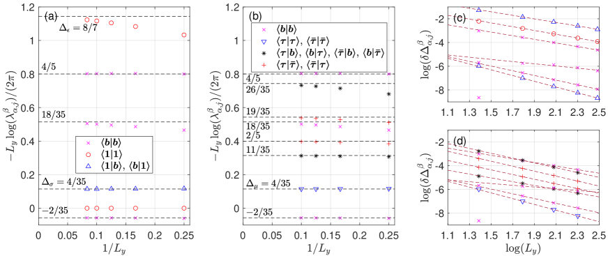
Figure 5: Numerically extracted scaling dimensions of primary fields in the DYL case. (a)-(b) Scaling dimensions $-L_{y}\log(\lambda_{\bm{\alpha},j}^{\bm{\beta}})/2\pi$ extracted numerically from $\mathbb{T}_{1}^{1}$ (left) and $\mathbb{T}_{\tau}^{\tau}$ (right) on cylinders with circumference $L_{y}$, where $\lambda_{\bm{\alpha},j}^{\bm{\beta}}$ are rescaled eigenvalues, classified into different topological sectors $\langle\bm{\alpha}|\bm{\beta}\rangle$. The dashed lines are the CFT predictions. $\Delta_{\sigma}$, $\Delta_{\epsilon}$ and $\Delta_{\mu}$ label the scaling dimensions of order parameters, energy, and disorder operators. (c)-(d) The finite-size corrections $\delta\Delta_{\bm{\alpha},j}^{\bm{\beta}}(L_{y})=|-L_{y}\log(\lambda_{\bm{\alpha},j}^{\bm{\beta}})/2\pi-\Delta_{\bm{\alpha},j}^{\bm{\beta}}|$ of the scaling dimensions extracted from $\mathbb{T}_{1}^{1}$ (above) and $\mathbb{T}_{\tau}^{\tau}$ (below) vanish algebraically with $L_{y}$, where $\Delta_{\bm{\alpha},j}^{\bm{\beta}}$ are the exact values predicted from CFT.

In analogy to the deformed DFib string-net wavefunction, the deformed Yang-Lee string-net wavefunction can also be obtained by acting with deformation operators on the $\{i_{1}\}$ and $\{i_{2}\}$ spins of a ground state wavefunction $|\Psi_{\text{DYL}}\rangle_{R}$ of the DYL string-net model:

$$|\Psi(K)\rangle_{R}=\prod_{i_{1}i_{2}}\exp\left[K(\sigma^{z}_{i_{1}}+\sigma^{z}_{i_{2}})/4\right]|\Psi_{\text{DYL}}\rangle_{R}.$$ (16)

The parent Hamiltonian for the fixed point model at $K=0$ is complex symmetric, $H=H^{T}$, and has a real spectrum [3], and thus, the left ground state eigenvector is the transpose of the right one, ${}_{L}\langle\Psi(0)|=\big{(}|\Psi(0)\rangle_{R}\big{)}^{T}$; we henceforth distinguish them by subscripts $L$ and $R$. While it is not clear how to modify the Hamiltonian for the DYL model such as to have $|\Psi(K)\rangle_{R}$ as its ground state [a modification analogous to Eq. (5) does not necessarily have positive spectrum, as $H(0)$ is not positive semi-definite], we anticipate that a suitable parent Hamiltonian should keep the property that ${}_{L}\langle\Psi(K)|=\big{(}|\Psi(K)\rangle_{R}\big{)}^{T}$, which we assume henceforth. Due to the non-Hermitian nature of the system (where the normalization condition imposes that left and right eigenvectors are biorthogonal), it is natural to consider the overlap ${}_{L}\langle\Psi(K)|\Psi(K)\rangle_{R}$, rather than the normalization of $|\Psi(K)\rangle_{R}$, when mapping the system to a statmech model, and correspondingly when constructing condensation and deconfinement order parameters by inserting MPOs, and we will do so in the following.

Since the DYL string-net wavefunction can be obtained from the DFib string-net wavefunction by substituting $\phi^{\prime}=-1/\phi$ for $\phi$, it is natural to expect that for the deformed DYL wavefunction, ${}_{L}\langle\Psi(K)|\Psi(K)\rangle_{R}$ can be mapped to the partition function of the $(\phi^{\prime}+2)$-state Potts model. In Appendix B, we prove – using the formulation in terms of tensor networks – that ${}_{L}\langle\Psi(K)|\Psi(K)\rangle_{R}$ for the deformed DYL wavefunction is exactly equivalent to the partition function of a non-unitary RSOS model associated with the $D_{6}$ Dynkin diagram. From there, we can again conclude from the Potts–RSOS equivalence [39] that this nonunitary RSOS model is in turn equivalent to the square lattice $(\phi^{\prime}+2)$-state Potts model. Thus, we have

$${}_{L}\langle\Psi(K)|\Psi(K)\rangle_{R}\propto\mathcal{Z}_{\text{Potts}}(\phi^{\prime}+2,K).$$ (17)

According to Eq. (7), the critical point of the $(\phi^{\prime}+2)$-state Potts model is located at $e^{K_{c}}=1+\sqrt{2+\phi^{\prime}}\approx 2.1756$ and is described by a non-unitary minimal CFT with a central charge $c=8/35$.

IV.2 Condensate and deconfinement fractions

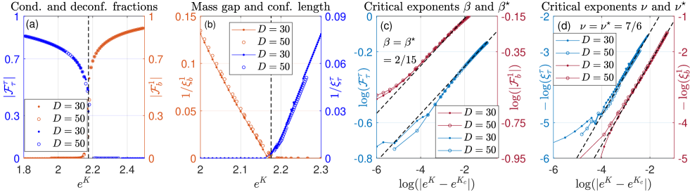
Figure 6: Numerical results for the DYL case. (a) Condensate fraction $|\mathcal{F}_{\bm{b}}^{\bm{1}}|$ and deconfinement fraction $|\mathcal{F}_{\bm{\tau}}^{\bm{\tau}}|$ for different bond dimensions $D$. the dashed line indicates the exact position of the critical point. (b) Anyon “mass gap” $1/\xi_{\bm{b}}^{\bm{1}}$ and inverse of the confinement length $1/\xi_{\bm{\tau}}^{\bm{\tau}}$. (c) Scaling of the $|\mathcal{F}_{\bm{b}}^{\bm{1}}|$ and $|\mathcal{F}_{\bm{\tau}}^{\bm{\tau}}|$ in the vicinity of the exact critical point. The slope of the dashed lines is the CFT prediction 2/15. (d) Scaling of $1/\xi_{\bm{\tau}}^{\bm{\tau}}$ and $1/\xi_{\bm{b}}^{\bm{1}}$ in the vicinity of the exact critical point. The slope of the dashed lines is the CFT prediction 7/6.

The condensate fraction for the Yang-Lee case is:

$$\mathcal{F}^{\bm{1}}_{\bm{b}}=\frac{{}_{L}\langle\bm{1}|\dot{\bm{b}}_{i}\rangle_{R}}{{}_{L}\langle\bm{1}|\bm{1}\rangle_{R}},$$ (18)

where $|\bm{1}\rangle$ is a MES and $|\dot{\bm{b}}_{i}\rangle_{R}$ is obtained by creating a $\bm{b}$ excitation on top of $|\bm{1}\rangle$. Since the left and right eigenvectors satisfy bi-orthogonality, the analysis is analogous to the one in the Fibonacci case. The condensate fraction $\mathcal{F}^{\bm{1}}_{\bm{b}}$ is zero in the topological phase and non-zero in the non-topological phase. Yet again, $\mathcal{F}^{\bm{1}}_{\bm{b}}$ and $\mathcal{F}^{\bm{b}}_{\bm{1}}$ can be mapped to the expectation values of the local order parameters of the RSOS model, as proved in Appendix B.

The deconfinement fraction is

$$\mathcal{F}_{\bm{\tau}}^{\bm{\tau}}=\frac{{}_{L}\langle\dot{\bm{\tau}}_{i}|\dot{\bm{\tau}}_{i}\rangle_{R}}{{}_{L}\langle\bm{1}|\bm{1}\rangle_{R}},$$ (19)

where the definition of $|\dot{\bm{\tau}}_{i}\rangle_{R}$ is the same as in the DFib case. Because the $\bm{\tau}$ anyons are chiral, the left eigenvector ${}_{L}\langle\dot{\bm{\tau}}_{i}|$ is not simply the transpose of the right eigenvector $|\dot{\bm{\tau}}_{i}\rangle_{R}$: Considering that an excitation carried by a left eigenvector should have a chirality opposite to that of the excitation carried by the corresponding right eigenvector, the proper definition of ${}_{L}\langle\bm{\tau}_{i}|$ is to insert an end tensor

$$E_{\bm{\tau}}(d_{i},F_{tsu}^{ijk},(R^{ij}_{k})^{\star})=E_{\bm{\bar{\tau}}}(d_{i},F_{tsu}^{ijk},R^{ij}_{k})$$ (20)

with an infinite long non-trivial MPO string attached to it into the PEPS ${}_{L}\langle\bm{1}|$. Again, the deconfinement fraction can be considered as a non-local disorder parameter for the $(\phi^{\prime}+2)$-state Potts model.

The correlation functions $\mathcal{C}_{\bm{b}}^{\bm{1}}$ and $\mathcal{C}_{\bm{\tau}}^{\bm{\tau}}$ in the DYL case are similar to those in the DFib case: $\mathcal{C}_{\bm{b}}^{\bm{1}}$ ($\mathcal{C}_{\bm{\tau}}^{\bm{\tau}}$) decays exponentially in the gapped topological (non-topological) phase:

$$\mathcal{C}_{\bm{b}}^{\bm{1}}(|i-j|) = \frac{{}_{L}\langle\bm{1}|\dot{\bm{b}}_{i}\dot{\bm{b}}_{j}\rangle_{R}}{{}_{L}\langle\bm{1}|\bm{1}\rangle_{R}}\propto\exp{\left(-\frac{|i-j|}{\xi^{\bm{1}}_{\bm{b}}}\right)},$$

$$\mathcal{C}_{\bm{\tau}}^{\bm{\tau}}(|i-j|) = \frac{{}_{L}\langle\dot{\bm{\tau}}_{i}\dot{\bm{\tau}}_{j}|\dot{\bm{\tau}}_{i}\dot{\bm{\tau}}_{j}\rangle_{R}}{{}_{L}\langle\bm{1}|\bm{1}\rangle_{R}}\propto\exp{\left(-\frac{|i-j|}{\xi_{\bm{\tau}}^{\bm{\tau}}}\right)},$$ (21)

where $|\dot{\bm{b}}_{i}\dot{\bm{b}}_{j}\rangle_{R}$ and $|\dot{\bm{\tau}}_{i}\dot{\bm{\tau}}_{j}\rangle_{R}$ are obtained by creating a pair of anyons on top of $|\bm{1}\rangle_{R}$, and the anyons in ${}_{L}\langle\dot{\bm{\tau}}_{i}\dot{\bm{\tau}}_{j}|$ carry the opposite chirality. Again, the scaling of these quantities close to criticality is given by scaling exponents $\beta$, $\nu$, $\eta$, and $\beta^{\star}$, $\nu^{\star}$, $\eta^{\star}$, as defined in Eqs. (13) and (14).

To predict the critical exponents from CFT, we proceed as the Fibonacci case. $\Delta_{\sigma}$ and $\Delta_{\epsilon}$ can be determined by known results for the corresponding RSOS and Potts models, as shown in Appendix B. Again, $\Delta_{\mu}$ can only be identified numerically from the spectrum of the transfer operator in the respective sector; the corresponding numerical results are discussed in Fig. 5(b) and Appendix C. Note that there is a negative scaling dimension $-2/35$ in the topological sector $\langle\bm{b}|\bm{b}\rangle$, signifying the non-unitarity of the CFT. In summary, we obtain

$$\Delta_{\sigma}=\Delta_{\mu}=4/35,\quad\Delta_{\epsilon}=8/7.$$ (22)

Notice that the duality (III.3) between different topological sectors is still satisfied for the DYL case. Assuming that the scaling relations $\Delta_{\sigma}=\eta/2,\Delta_{\epsilon}=2-1/\nu,\beta=\eta\nu/2$ are still valid for this non-Hermitian model, the critical exponents are obtained as:

$$\eta=8/35,\quad\nu=7/6,\quad\beta=2/15.$$ (23)

From duality, we expect the dual critical exponents $\eta^{\star}$, $\mu^{\star}$ and $\beta^{\star}$ to be equal to $\eta$, $\mu$ and $\beta$, respectively.

IV.3 Numerical results

The predictions and expectations above can be verified numerically by computing the topological order and disorder parameters. Because in the DYL case the transfer operator is non-Hermitian, the VUMPS method cannot be reliably used, and we resort to CTMRG instead. Fig. 6(a) shows the condensate fraction $|\mathcal{F}_{\bm{b}}^{\bm{1}}|$ and the deconfinement fractions $|\mathcal{F}_{\bm{\tau}}^{\bm{\tau}}|$ calculated using different bond dimensions $D$ of the CTM environments. The position of the critical point implied by the fractions matches the exact value $e^{K_{c}}=1+\sqrt{2+\phi^{\prime}}\approx 2.1756$. Fig. 6 (c) displays the scaling of condensate and deconfinement fractions, and the slopes of the data which are converged in $D$ are in good agreement with critical exponents $\beta=\beta^{\star}=2/15$ predicted from CFT. Fig. 6 (b) shows the “mass gap” and the inverse of the confinement length, and Fig. 6 (d) shows their scaling close to criticality, which is again in good agreement with the analytically derived critical exponents $\nu=\nu^{\star}=7/6$.

V Conclusion and discussion

In this work, we have generalized order parameters for condensation and deconfinement of anyons to the case of non-Abelian topological models, including no-Hermitian ones. In particular, we have focused on the DFib string-net model and its Galois conjugate, the DYL string-net model. We proved that the normalization of the string tension deformed DFib and DYL string-net states are equivalent to partition functions of $D_{6}$ RSOS models, and based on this we proved the equivalence of the condensate fraction to the order parameter of the RSOS models. We have used this equivalence to predict critical exponents related to the condensation and deconfinement order parameters, and we have confirmed these predictions by numerical studies.

Our approach can be straightforwardly applied to other non-Abelian string-net models. An interesting additional aspect beyond condensation and confinement of anyons, which arises in topological phase transitions in more complex models, is the fact that one non-Abelian anyon can split into different kinds of anyons at the transition [19, 49]. It is an interesting question whether and how to construct an order parameter that directly detects this splitting. A different question is how to generalize our approach to variationally opimized PEPS obtained from tuning a Hamiltonian, rather than from explicitly constructed wavefunction families. To this end, one could use either a constrained optimization on the manifold of MPO-symmetric tensors [21], or methods developed to extract the MPO symmetry a posteriori from an optimized PEPS tensor [31]. It is an interesting open question to construct and investigate condensation and deconfinement order parameters in such a scenario.

Appendix A Definitions of all tensors

All tensors can be defined using $d_{i},N_{ij}^{k},F^{ijk}_{tsu}$ and $R^{ij}_{k}$. The $d$ tensor has already been defined in the main text. The non-zero entries of the $N$ tensor are $N_{11}^{1}=N_{1\tau}^{\tau}=N_{\tau 1}^{\tau}=N_{\tau\tau}^{1}=N_{\tau\tau}^{\tau}=1$. The non-zero entries of the $F$ tensor are determined by $N_{ij}^{k}$, i.e., $F^{ijk}_{tsu}\neq 0$ if $N_{ij}^{k}N_{ts}^{k}N_{is}^{u}N_{jt}^{u}=1$. For the DFib and DYL cases, the nontrivial entries are given by Eqs. (2) and (3), separately, and other non-zero entries are $1$. From the $F$ tensor, it is convenient to define the $G$ tensor:

$$G^{ijk}_{\alpha\beta\gamma}=F^{ijk}_{\alpha\beta\gamma}/\sqrt{d_{k}d_{\gamma}}=\includegraphics[width=42.67912pt,valign={c}]{Tetrahedra.pdf}.$$ (24)

The $G$ tensor has tetrahedral symmetry so we can also represent it using a tetrahedron. A triple-line local tensor generating the PEPS of a string-net wavefunction can be expressed as[5, 6]:

$$\includegraphics[width=56.9055pt,valign={c}]{PEPS_local_tensor.pdf}=(d_{i}d_{j}d_{k})^{\frac{1}{4}}G^{ijk}_{\alpha\beta\gamma}$$ (25)

where the open circles represent the physical degrees of freedom and the lines are virtual degrees of freedom. Each line represents a $\delta$ tensor, i.e., the entries are non-zero iff all of its indices are equal. In the PEPS representation of the string-net wavefunctions, there is a convention that the contraction of the degrees of freedom is a sum weighted by the quantum dimenisons, so we should assign the weight $d_{\alpha}^{\frac{1}{6}},d_{\beta}^{\frac{1}{6}}$ and $d_{\gamma}^{\frac{1}{6}}$ to $\alpha$, $\beta$ and $\gamma$ indices of the tensor in (25), but we omit them after and in the next for convenience. The local tensor on the square lattice is obtained by contracting the above two tensors:

(26)

The local tensor of the horizontal MPO $O_{n}$ is[9]:

$$\includegraphics[width=85.35826pt,valign={c}]{MPO_tensor.pdf}=G_{lmn}^{ijk},$$ (27)

where $n=1$ or $\tau$ is a fixed index. In the abbreviated graphs, the red (blue) lines represent the triple-line (double-line) in the original graphs, and the horizontal MPO can be generated by the tensor:

$$\includegraphics[width=128.0374pt,valign={c}]{MPO_appendix.pdf}.$$ (28)

Furthermore, by defining the tensor with the fixed indices $i,j$ and $k$:

$$\includegraphics[width=113.81102pt,valign={c}]{Crossing_tensor.pdf}=G^{ijk}_{dcb}G^{jki}_{dac},$$ (29)

a vertical MPO $O_{ikj}$ can be generated together with the tensor (it should be rotated by $\pi/2$) in Eq. (27):

$$O_{ikj}=\includegraphics[width=28.45274pt,valign={c}]{MPO.pdf}.$$ (30)

Notice that the up and down legs are connected periodically. These vertical MPOs form a basis of the tube algebra. The following linear combinations of the vertical MPOs are the central idempotents of the tube algebra:

$$P_{\bm{\alpha}}=\frac{d_{a}d_{b}}{d_{1}^{2}+d_{\tau}^{2}}\sum_{ikj}d_{j}d_{k}C_{ikj}(a,b)O_{ikj},\\$$ (31)

where indices $(a,b)$ are determined by $\bm{\alpha}$:

$$\bm{1}=(1,1),\quad\bm{\tau}=(\tau,1),\quad\bm{\bar{\tau}}=(1,\tau),\quad\bm{b}=(\tau,\tau),$$ (32)

and

$$C_{ikj}(a,b)=\sum_{\gamma\delta}d_{\gamma}d_{\delta}R^{aj}_{\gamma}R^{jb}_{\delta}G^{i\delta\gamma}_{jab}G^{ka\delta}_{bji}G^{ikj}_{a\gamma\delta}.$$ (33)

The explicit expressions of the idempotents for the DFib and DYL cases can be found in Refs. [34] and [27], respectively. The non-zero entries of $R$ tensor are

$$R_{1}^{11} = R_{\tau}^{1\tau}=R_{\tau}^{\tau 1}=1,$$

$$R_{1}^{\tau\tau} = \begin{cases}e^{4\pi i/5},&\text{DFib }\\ e^{2\pi i/5},&\text{DYL }\end{cases},\quad R_{\tau}^{\tau\tau}=\begin{cases}e^{-3\pi i/5},&\text{DFib }\\ e^{\pi i/5},&\text{DYL }\end{cases}.$$

Since $C_{\tau kj}(1,1)=C_{1kj}(1,\tau)=C_{1kj}(\tau,1)=0$, we have

$$P_{\bm{1}}=P_{\bm{1}1},\quad P_{\bm{\tau}}=P_{\bm{\tau}\tau},\quad P_{\bm{\bar{\tau}}}=P_{\bm{\bar{\tau}}\tau},\quad P_{\bm{b}}=P_{\bm{b}1}\oplus P_{\bm{b}\tau}.$$ (34)

The end tensor carrying anyonic excitations is defined as[34]

$$E_{\bm{\alpha}k}=\includegraphics[width=113.81102pt,valign={c}]{end_tensor.pdf}$$

$$=d_{a}^{\frac{1}{4}}d_{b}^{\frac{1}{4}}d_{x}^{\frac{1}{4}}d_{y}^{\frac{1}{4}}d_{k}\sum_{\beta}d_{\beta}C_{k\beta w}(a,b)G^{u\beta x}_{wvk}G_{x\beta k}^{wyu}.$$

Appendix B Mapping the deformed PEPS to the RSOS models

The norms of the string-net wavefunctions can be exactly mapped to the partition function of the RSOS models, from which we know the positions of critical points and the CFTs describing the critical points. Furthermore, we can also find that the condensate fractions are exactly the same as the expectation values of the RSOS order parameters, from which one can find the critical exponents related to the condensate fractions.

At first we consider a local double tensor for the norm of the DFib or DYL PEPS without the deformation:

$$\sum_{k}d_{k}\includegraphics[width=71.13188pt,valign={c}]{double_tensor_1.pdf}=\sum_{k}d_{k}G^{ijk}_{tsu}G^{klm}_{wts}G^{ijk}_{t^{\prime}s^{\prime}u^{\prime}}G^{klm}_{w^{\prime}t^{\prime}s^{\prime}}.$$ (36)

Since the $F$-move gives rise to the following relation:

$$\sum_{k}d_{k}\includegraphics[width=71.13188pt,valign={c}]{double_tensor_1.pdf}=\sum_{n}d_{n}\includegraphics[width=71.13188pt,valign={c}]{double_tensor_2.pdf},$$ (37)

the tensor in (36) actually respects the symmetry described the dihedral group $D_{4}$. In addition, because the $G$ tensor has the tetrahedral symmetry, the relation (37) can also be represented by the tetrahedrons:

$$\sum_{k}d_{k}\includegraphics[width=62.59596pt,valign={c}]{Tetrahedra_1.pdf}=\sum_{n}d_{n}\includegraphics[width=62.59596pt,valign={c}]{Tetrahedra_2.pdf},$$ (38)

where each $G$ tensor is represented by a tetrahedron.

In this tetrahedral representation, one can easily find the following relation:

$$\sum_{k}d_{k}\includegraphics[width=62.59596pt,valign={c}]{Tetrahedra_1.pdf}=\sum_{x}d_{x}\includegraphics[width=62.59596pt,valign={c}]{Tetrahedra_3.pdf}.$$ (39)

Namely

$$\sum_{k}d_{k}G^{ijk}_{tsu}G^{klm}_{wts}G^{ijk}_{t^{\prime}s^{\prime}u^{\prime}}G^{klm}_{w^{\prime}t^{\prime}s^{\prime}}$$ (40)

$$= \sum_{x}d_{x}G^{utj}_{t^{\prime}u^{\prime}x}G^{twm}_{w^{\prime}t^{\prime}x}G^{wsl}_{s^{\prime}w^{\prime}x}G^{sui}_{u^{\prime}s^{\prime}x}.$$

So a double tensor at a vertex of the lattice is decomposed into four $G$ tensors living seperately on the four edges:

$$\sum_{k}d_{k}\includegraphics[width=71.13188pt,valign={c}]{double_tensor_1.pdf}=\sum_{x}d_{x}\includegraphics[width=71.13188pt,valign={c}]{double_tensor_3.pdf}.$$ (41)

Since the two nearest neighboring original double tensors share a common edge, there are two $G$ tensors on each edge after the decomposition (41), and we can contract them together with the string tension deformation $T=(e^{K/2},e^{-K/2})$:

$$\sum_{i}d_{i}G^{sui}_{u^{\prime}s^{\prime}x}G^{usi}_{s^{\prime}u^{\prime}y}T_{i}=\sum_{i}d_{i}G^{sui}_{u^{\prime}s^{\prime}x}G^{sui}_{u^{\prime}s^{\prime}y}T_{i}$$ (42)

$$= e^{-K/2}\left(G^{su1}_{u^{\prime}s^{\prime}x}G^{su1}_{u^{\prime}s^{\prime}y}e^{K}+d_{\tau}G^{su\tau}_{u^{\prime}s^{\prime}x}G^{su\tau}_{u^{\prime}s^{\prime}y}\right)$$

$$= e^{-K/2}\left[G^{su1}_{u^{\prime}s^{\prime}x}G^{su1}_{u^{\prime}s^{\prime}y}(e^{K}-1)+\sum_{i}d_{i}G^{sui}_{u^{\prime}s^{\prime}x}G^{sui}_{u^{\prime}s^{\prime}y}\right]$$

$$= e^{-K/2}\left[\frac{\delta_{ss^{\prime}}\delta_{uu^{\prime}}}{d_{s}d_{u}}(e^{K}-1)+\frac{\delta_{xy}}{d_{x}}\right]N_{ss^{\prime}}^{x}N_{uu^{\prime}}^{y}$$

$$= \frac{\sqrt{q}}{e^{K/2}}\left(\frac{\delta_{ss^{\prime}}\delta_{uu^{\prime}}}{d_{s}d_{u}}\frac{e^{K}-1}{\sqrt{q}}+\frac{\delta_{xy}}{d_{x}\sqrt{q}}\right)N_{ss^{\prime}}^{x}N_{uu^{\prime}}^{y}.$$

As shown in Fig. 7 (a), the tensor in (42) is represented by the gray rectangles, and in the following, we will explain that the tensor network in Fig. 7 (a) is merely one of the RSOS models.

As displayed in Fig. 7 (b), the red lines in Fig. 7 (a) are the degrees of freedom living on the sites of the primal square lattice and they takes two values $1$ and $\tau$. The blue and purple lines in Fig. 7 (a) are the degrees of freedom living on the sites of the dual square lattice and they takes four values $(1,1)$, $(\tau,\tau)$, $(1,\tau)$ and $(\tau,1)$. All of them are degrees of freedom of the RSOS models, which live on the medial lattice shown in 7 (b). The nearest neighboring degrees of freedom of the RSOS models are restricted by two $N$ tensors in the last line of Eq. (42). And this restriction can be represented by the following $D_{6}$ Dynkin diagram[38, 50, 51, 22]:

$$\includegraphics[width=113.81102pt,valign={c}]{Dynkin_diagram.pdf}.$$ (43)

This means that the two degrees of freedom of the RSOS models can be nearest neighboring if and only if they are adjacent in the Dynkin diagram. The nodes of the diagram are denoted by $h$, which are called heights of the RSOS models, and they take the six values $(1,1),1,(\tau,\tau),\tau,(1,\tau),(\tau,1)$. The Dynkin diagram imposes the restriction on the medial lattice and naturally divides the medial lattice into two sublattices, which are the primal lattice and the dual lattice. And the Dynkin diagram defines not only the configurations of the RSOS models but also their Boltzmann weights, as shown in the following.

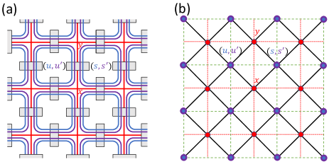
Figure 7: (a) A tensor network representation for the RSOS models. (b) The degrees of freedom of the RSOS models are represented by dots. The red/green/black lines form the primal/dual/medial lattice.

At first we consider an adjacency matrix describing the Dynkin diagram (43):

$$\mathcal{A}=\left(\begin{array}[]{cccccc}0&1&0&0&0&0\\ 1&0&1&0&0&0\\ 0&1&0&1&0&0\\ 0&0&1&0&1&1\\ 0&0&0&1&0&0\\ 0&0&0&1&0&0\\ \end{array}\right).$$ (44)

Its eigenvalues are $2\cos(r\pi/p)$, where $p=10$ is the Coxeter number for the $D_{6}$ Dynkin diagram and $r=1,3,5,7,9$. The corresponding eigenvectors $S^{(r)}$ are

$$S^{(1)} = (1,\sqrt{\phi+2},\phi^{2},\phi\sqrt{\phi+2},\phi,\phi)^{T},$$

$$S^{(3)} = (1,\sqrt{\phi^{\prime}+2},\phi^{\prime 2},\phi^{\prime}\sqrt{\phi^{\prime}+2},\phi^{\prime},\phi^{\prime})^{T},$$

$$S^{(\bar{5})} = (1,0,-1,0,\phi,\phi^{\prime})^{T},$$

$$S^{(5)} = (1,0,-1,0,\phi^{\prime},\phi)^{T},$$

$$S^{(7)} = (1,-\sqrt{\phi^{\prime}+2},\phi^{\prime 2},-\phi^{\prime}\sqrt{\phi^{\prime}+2},\phi^{\prime},\phi^{\prime})^{T},$$

$$S^{(9)} = (1,-\sqrt{\phi+2},\phi^{2},-\phi\sqrt{\phi+2},\phi,\phi)^{T}.$$

The eigenvalue $0$ is two-fold degenerate, so we distinguish the corresponding two eigenvectors $S^{(5)}$ and $S^{(\bar{5})}$.

There are two different RSOS models. One is defined using $S=S^{(1)}$, and the other one is defined using $S=S^{(3)}$. The partition functions of the RSOS models can be expressed in terms of the adjacency matrix $\mathcal{A}$ and $S$:

$$\mathcal{Z}_{\text{RSOS}}=\sum_{\{h_{i}\}}\prod_{\langle h_{i}h_{j}\rangle}\mathcal{A}_{h_{i},h_{j}}\prod_{i}S_{h_{i}}\prod_{\diamond}W_{\diamond},$$ (46)

where

$$W_{\diamond} = W(\includegraphics[width=42.67912pt,valign={c}]{RSOS_boltzmann_weight.pdf})=\frac{\delta_{h_{1}h_{3}}}{S_{h_{1}}}\frac{e^{K}-1}{\sqrt{q}}+\frac{\delta_{h_{2}h_{4}}}{S_{h_{2}}}$$

or $$W(\includegraphics[width=42.67912pt,valign={c}]{RSOS_boltzmann_weight_2.pdf})=\frac{\delta_{h_{2}h_{4}}}{S_{h_{2}}}\frac{e^{K}-1}{\sqrt{q}}+\frac{\delta_{h_{1}h_{3}}}{S_{h_{1}}}$$

are the Boltzmann weights defined on the plaquettes of the medial lattice. It can be found that Eq. (B) is exactly equivalent to the last row of Eq. (42), and $S=S^{(1)}$ ($S=S^{(3)}$) corresponds to the DFib (DYL) case. Notice that when we contract the tensor network, we add weights $d_{i}$ to the degrees of freedom which will be contracted. The weights are equivalent to the term $\prod_{i}S_{h_{i}}$ in Eq. (46). So an exactly relation between the norms of the PEPS and the partition functions of the RSOS model can be established:

$$\mathcal{Z}=(qe^{-K})^{\#\text{site}/4}\mathcal{Z}_{\text{RSOS}},$$ (48)

where $\mathcal{Z}=\langle\Psi(K)|\Psi(K)\rangle$ in the DFib case and $\mathcal{Z}={}_{L}\langle\Psi(K)|\Psi(K)\rangle_{R}$ in the DYL case, and $\#\text{site}$ is the number of sites of the medial lattice.

It has been proved that the partition functions of RSOS models constructed using $S^{(r)}$ are equivalent to that of $q$-state Potts models with $q=4\cos^{2}(r\pi/p)$[39], where $p$ is the Coxeter number of the Dynkin diagram. So, in the DFib case, the RSOS model is equivalent to the $(\phi+2)$-state Potts model, and this is consistent with the well-known results[28, 29]. In the DYL case, the RSOS model is equivalent to the $(\phi^{\prime}+2)$-state Potts model. When $e^{K}=1+\sqrt{q}$, the RSOS models are critical. The central charges of the CFTs describing the critical points are $c=1-6r^{2}/[p(p-r)]$, where $p=10$ and $r=1$ ($r=3$) for the DFib (DYL) case.

Moreover, the order parameters of the RSOS models can be defined as $S^{(5)}_{h}/S_{h}$ and $S^{(\bar{5})}_{h}/S_{h}$[43, 38, 39], where the denominator $S_{h}$ cancels the weights assigned previously and the numerator assigns new weights. At the critical points, the scaling dimensions of the RSOS order parameters are given by

$$\Delta_{\sigma}=\frac{(p/2)^{2}-r^{2}}{2p(p-r)}.$$ (49)

So in the DFib (DYL) case $\Delta_{\sigma}=2/15$ ($4/35$). In addition, although it is tricky to talk about the definition of Potts order parameters when $q$ is not an integer, the scaling dimensions $\Delta_{\sigma}$ and $\Delta_{\epsilon}$ of the Potts models are known as a function of $q$[44]:

$$\Delta_{\sigma}=\frac{\delta^{2}-4}{8\delta(\delta-1)},\quad\Delta_{\epsilon}=\frac{\delta+2}{2(\delta-1)},$$ (50)

where $q=4\cos^{2}(\pi/\delta)$. So we say that the scaling dimensions of the RSOS order parameters coincide with those of the Potts order parameters.

Furthermore, because in the procedures of mapping tensor networks to the RSOS models, the virtual loops around the plaquettes remain unchanged and they are equivalent to the heights on the dual lattice (one sublattice of the medial lattice). It can therefore be proved that the expectation values of the RSOS order parameters are equivalent to the condensate fractions. At first according to Eq. (A), one can check that

$$E_{\bm{b}1}=d_{\tau}^{1/2}\delta_{uv}\delta_{xy}d_{v}^{-1/4}d_{u}^{-1/4}d_{w}^{-2}(-1)^{\delta_{w\tau}}.$$ (51)

The term $d_{v}^{-1/4}d_{u}^{-1/4}$ cancels the weights assigned to $u$ and $v$, which arise from the convention of contraction. The term $d_{w}^{-2}(-1)^{\delta_{w\tau}}$ cancels the weight $d_{w}$ previously assigned to virtual loop $w$ and assigns a new weight $(-1)^{\delta_{w\tau}}/d_{w}$ to $w$. So inserting $E_{\bm{b}1}$ into the PEPS just locally modifies the weight on virtual loops $w$ from $(1,d_{\tau})$ to $(1,-1/d_{\tau})$. Taking the loop $w^{\prime}$ in another layer into consideration, for the DFib case we replace the original weights $(1,d_{\tau})\otimes(1,d_{\tau})=(1,d_{\tau},d_{\tau},d_{\tau}^{2})$ with

$$(1,d_{\tau})\otimes(1,-\frac{1}{d_{\tau}}) = (S^{(5)}_{1},S^{(5)}_{5},S^{(5)}_{6},S^{(5)}_{3})\quad\text{or}$$

$$(1,-\frac{1}{d_{\tau}})\otimes(1,d_{\tau}) = (S^{(\bar{5})}_{1},S^{(\bar{5})}_{5},S^{(\bar{5})}_{6},S^{(\bar{5})}_{3}),$$

and for the DYL case we replace the original weights with

$$(1,d_{\tau})\otimes(1,-\frac{1}{d_{\tau}}) = (S^{(\bar{5})}_{1},S^{(\bar{5})}_{5},S^{(\bar{5})}_{6},S^{(\bar{5})}_{3})\quad\text{or}$$

$$(1,-\frac{1}{d_{\tau}})\otimes(1,d_{\tau}) = (S^{(5)}_{1},S^{(5)}_{5},S^{(5)}_{6},S^{(5)}_{3}).$$

Because of the above equations, we can therefore identify that inserting the $E_{\bm{b}1}$ shown in (51) into the tensor networks is exactly equivalent to evaluating order parameters $S^{(5)}_{h}/S_{h}$ and $S^{(\bar{5})}_{h}/S_{h}$. Therefore the condensate fractions are exactly equivalent to the expectation values of RSOS order parameters:

$$\mathcal{F}_{\bm{1}}^{\bm{b}}=\mathcal{F}_{\bm{b}}^{\bm{1}}\propto\left\langle\frac{S^{(5)}_{h_{i}}}{S_{h_{i}}}\right\rangle_{\mathcal{Z}_{\text{RSOS}}}=\left\langle\frac{S^{(5^{\prime})}_{h_{i}}}{S_{h_{i}}}\right\rangle_{\mathcal{Z}_{\text{RSOS}}},$$ (52)

where $\langle\bullet\rangle_{\mathcal{Z}_{\text{RSOS}}}$ denotes the thermal ensemble average.

Appendix C Topological sectors of the transfer operator and form factors of the correlation functions

The form factors together with the transfer operators determine the correlation lengths of different kinds of correlation functions. On an infinitely long cylinder, the repeating units of the norms of the PEPS in Figs. 1 (a) and (b) are the transfer operators $\mathbb{T}_{1}^{1}$ and $\mathbb{T}_{\tau}^{\tau}$ with the closed boundary conditions, see Fig. 2 (b). Since the PEPS in Fig.1 (a) and (b) are equal to $|\bm{1}\rangle+|\bm{b}\rangle$ and $|\bm{b}\rangle+|\bm{\tau}\rangle+|\bm{\bar{\tau}}\rangle$ individually, their transfer operators $\mathbb{T}_{1}^{1}$ and $\mathbb{T}_{\tau}^{\tau}$ contain 4 and 9 topological sectors seperately. These topological sectors are subblock transfer operators of the MES overlaps: $\langle\bm{\alpha}|\bm{\beta}\rangle$, where $\bm{\alpha},\bm{\beta}=\bm{1},\bm{\tau},\bar{\bm{\tau}},\bm{b}$. Using the idempotents in Eq. (34), the projectors $\mathbb{P}_{\bm{\alpha}}^{\bm{\beta}}=P_{\bm{\beta}1}\otimes P_{\bm{\alpha}1}$ and $\mathbb{\tilde{P}}_{\bm{\alpha}}^{\bm{\beta}}=P_{\bm{\bar{\beta}}\tau}\otimes P_{\bm{\alpha}\tau}$ (notice that the idempotents acting on bra and ket layers should have opposite chiralities) can be defined, the superscript (subscript)of $\mathbb{P}_{\bm{\alpha}}^{\bm{\beta}}$ stands for the MES in the bra (ket) layer. And by using the $\mathbb{P}_{\bm{\alpha}}^{\bm{\beta}}$, the subblocks of the trasfer operators can be projected out:

$$\mathbb{P}_{\bm{\alpha}}^{\bm{\beta}}\mathbb{T}_{1}^{1}\mathbb{P}_{\bm{\alpha}}^{\bm{\beta}} = \mathbb{T}_{1}^{1}\mathbb{P}_{\bm{\alpha}}^{\bm{\beta}}=\mathbb{P}_{\bm{\alpha}}^{\bm{\beta}}\mathbb{T}_{1}^{1},\quad\bm{\alpha},\bm{\beta}=\bm{1},\bm{b}$$

$$\mathbb{\tilde{P}}_{\bm{\alpha}}^{\bm{\beta}}\mathbb{T}_{\tau}^{\tau}\mathbb{\tilde{P}}_{\bm{\alpha}}^{\bm{\beta}} = \mathbb{T}_{\tau}^{\tau}\mathbb{\tilde{P}}_{\bm{\alpha}\tau}^{\bm{\beta}\tau}=\mathbb{\tilde{P}}_{\bm{\alpha}}^{\bm{\beta}}\mathbb{T}_{\tau}^{\tau},\quad\bm{\alpha},\bm{\beta}=\bm{b},\bm{\tau},\bm{\bar{\tau}}.$$ (53)

So the eigenvalues and eigenvectors of $\mathbb{T}_{1}^{1}$ and $\mathbb{T}_{\tau}^{\tau}$ can be classified into different topological sectors. By diagonalizing the transfer operators, we have

$$\mathbb{T}^{1}_{1} = \sum_{\bm{\alpha},\bm{\beta}=\bm{1},\bm{b}}\sum_{i}\lambda_{\bm{\alpha},i}^{\bm{\beta}}|r_{\bm{\alpha},i}^{\bm{\beta}})(l_{\bm{\alpha},i}^{\bm{\beta}}|,$$ (54)

$$\mathbb{T}^{\tau}_{\tau} = \sum_{\bm{\alpha},\bm{\beta}=\bm{b},\bm{\tau},\bm{\bar{\tau}}}\sum_{i}\lambda_{\bm{\alpha},i}^{\bm{\beta}}|\tilde{r}_{\bm{\alpha},i}^{\bm{\beta}})(\tilde{l}_{\bm{\alpha},i}^{\bm{\beta}}|,$$ (55)

where $\lambda_{\bm{\alpha},j}^{\bm{\beta}}$ is the $(j+1)$-th dominant eigenvalue of the topological sector $\langle\bm{\alpha}|\bm{\beta}\rangle$ (the spectrum is rescaled such that $\lambda_{\bm{1},0}^{\bm{1}}=1$ for convenience), and the left and right eigenvectors are bi-orthogonal:

$$(l_{\bm{\alpha},i}^{\bm{\beta}}|r_{\bm{\alpha}^{\prime},j}^{\bm{\beta}^{\prime}})=\delta_{\bm{\alpha}\bm{\alpha}^{\prime}}\delta_{\bm{\beta}\bm{\beta}^{\prime}}\delta_{ij},\quad(\tilde{l}_{\bm{\alpha},i}^{\bm{\beta}}|\tilde{r}_{\bm{\alpha}^{\prime},j}^{\bm{\beta}^{\prime}})=\delta_{\bm{\alpha}\bm{\alpha}^{\prime}}\delta_{\bm{\beta}\bm{\beta}^{\prime}}\delta_{ij}.$$ (56)

The dominant eigenvalue $\lambda_{\bm{\alpha},0}^{\bm{\beta}}$ of each topological sector is non-degenerate. And the eigenvalues $\lambda_{\bm{b},i}^{\bm{b}}$ from $\mathbb{T}_{1}^{1}$ and $\lambda_{\bm{b},i}^{\bm{b}}$ from $\mathbb{T}_{\tau}^{\tau}$ are equal, as shown in Figs. 3 (a) and (b) (also in Figs. 5 (a) and (b)).

On an infinitely long cylinder, the correlation function (10) can be expressed as:

$$\mathcal{C}_{\bm{b}}^{\bm{1}}(m) = (l_{\bm{1},0}^{\bm{1}}|(\mathbb{E}^{\bm{1}}_{\bm{b}})^{\text{T}}(\mathbb{T}^{1}_{1})^{m}\mathbb{E}^{\bm{1}}_{\bm{b}}|r_{\bm{1},0}^{\bm{1}})$$

$$= \sum_{\bm{\alpha},\bm{\beta}=\bm{1},\bm{b}}\sum_{i}(\lambda_{\bm{\alpha},i}^{\bm{\beta}})^{m}(l_{\bm{1},0}^{\bm{1}}|(\mathbb{E}^{\bm{1}}_{\bm{b}})^{\text{T}}|r_{\bm{\alpha},i}^{\bm{\beta}})(l_{\bm{\alpha},i}^{\bm{\beta}}|\mathbb{E}^{\bm{1}}_{\bm{b}}|r_{\bm{1},0}^{\bm{1}}),$$

where $\mathbb{E}^{\bm{1}}_{\bm{b}}$ is obtained by inserting an end tensor $E_{\bm{b}1}$ into the ket layer of the transfer operator $\mathbb{T}^{1}_{1}$, see Fig. 2 (c). The denominator of Eq. (10) disappears due to $\lambda_{\bm{1},0}^{\bm{1}}=1$. Because the $\mathbb{E}^{\bm{1}}_{\bm{b}}|r_{\bm{1},0}^{\bm{1}})$ is a vector belonging to the topological sector $\langle\bm{1}|\bm{b}\rangle$, the form factors of the correlation function satisfies:

$$(l_{\bm{\alpha},i}^{\bm{\beta}}|\mathbb{E}^{\bm{1}}_{\bm{b}}|r_{\bm{1},0}^{\bm{1}})\propto\delta_{\bm{\beta 1}}\delta_{\bm{\alpha b}}.$$ (57)

Therefore, the correlation function can be further simplified:

$$\mathcal{C}_{\bm{b}}^{\bm{1}}(m) = \sum_{i}(\lambda_{\bm{b},i}^{\bm{1}})^{m}(l_{\bm{1},0}^{\bm{1}}|(\mathbb{E}^{\bm{1}}_{\bm{b}})^{\text{T}}|r_{\bm{b},i}^{\bm{1}})(l_{\bm{b},i}^{\bm{1}}|\mathbb{E}^{\bm{1}}_{\bm{b}}|r_{\bm{1},0}^{\bm{1}})$$ (58)

$$\approx (\lambda_{\bm{b},0}^{\bm{1}})^{m}(l_{\bm{1},0}^{\bm{1}}|(\mathbb{E}^{\bm{1}}_{\bm{b}})^{\text{T}}|r_{\bm{b},0}^{\bm{1}})(l_{\bm{b},0}^{\bm{1}}|\mathbb{E}^{\bm{1}}_{\bm{b}}|r_{\bm{1},0}^{\bm{1}})$$

$$\propto \exp(-m/\xi_{\bm{b}}^{\bm{1}}),$$

where the approximation in the second line is valid for large $m$ and $1/\xi_{\bm{b}}^{\bm{1}}=-\log(\lambda_{\bm{b},0}^{\bm{1}})$. At the critical point, the eigenvalues of the transfer operators are also related to the scaling dimensions of CFT [52],

$$\Delta_{\bm{\alpha},j}^{\bm{\beta}}=-L_{y}\log\left(\lambda_{\bm{\alpha},j}^{\bm{\beta}}\right)/(2\pi)+\mathcal{O}(L_{y}^{-\gamma_{\bm{\alpha},j}^{\bm{\beta}}}),$$ (59)

where $L_{y}$ is the circumference of the transfer operators, $\gamma_{\bm{\alpha},j}^{\bm{\beta}}>0$ and the finite size corrections vanish with $L_{y}$ increasing, as shown in Figs. 3 (c) and (d) (also in Figs. 5 (c) and (d)). Hence we can numerically identify the scaling dimension $\Delta_{\sigma}=\Delta_{\bm{b},0}^{\bm{1}}$.

The correlation function (11) can be written as

$$\mathcal{C}_{\bm{\tau}}^{\bm{\tau}}(m) = (l_{\bm{1},0}^{\bm{1}}|(\mathbb{E}^{\bm{\bar{\tau}}}_{\bm{\bar{\tau}}})^{\text{T}}(\mathbb{T}^{\tau}_{\tau})^{m}\mathbb{E}^{\bm{\tau}}_{\bm{\tau}}|r_{\bm{1},0}^{\bm{1}})$$

$$= \sum_{\begin{subarray}{c}\bm{\alpha},\bm{\beta}=\\ \bm{b},\bm{\tau},\bm{\bar{\tau}}\end{subarray}}\sum_{i}(\lambda_{\bm{\alpha},i}^{\bm{\beta}})^{m}(l_{\bm{1},0}^{\bm{1}}|(\mathbb{E}^{\bm{\bar{\tau}}}_{\bm{\bar{\tau}}})^{\text{T}}|\tilde{r}_{\bm{\alpha},i}^{\bm{\beta}})(\tilde{l}_{\bm{\alpha},i}^{\bm{\beta}}|\mathbb{E}^{\bm{\tau}}_{\bm{\tau}}|r_{\bm{1},0}^{\bm{1}}),$$

where $\mathbb{E}^{\bm{\tau}}_{\bm{\tau}}$ is obtained by inserting the end tensors $E_{\bm{\bar{\tau}}\tau}$ and $E_{\bm{\tau}\tau}$ into the bra and ket layers of transfer operator $\mathbb{T}_{1}^{1}$, see Fig. 2 (d). Because the form factors have the following property:

$$(\tilde{l}_{\bm{\alpha},i}^{\bm{\beta}}|\mathbb{E}^{\bm{\tau}}_{\bm{\tau}}|r_{\bm{1},0}^{\bm{1}})\propto\delta_{\bm{\alpha\tau}}\delta_{\bm{\beta\tau}}.$$ (60)

The corrlation function can be simplified for the sufficient large $m$:

$$\mathcal{C}_{\bm{\tau}}^{\bm{\tau}}(m) = \sum_{i}(\lambda_{\bm{\tau},i}^{\bm{\tau}})^{m}(l_{\bm{1},0}^{\bm{1}}|(\mathbb{E}^{\bm{\bar{\tau}}}_{\bm{\bar{\tau}}})^{\text{T}}|\tilde{r}_{\bm{\tau},i}^{\bm{\tau}})(\tilde{l}_{\bm{\tau},i}^{\bm{\tau}}|\mathbb{E}^{\bm{\tau}}_{\bm{\tau}}|r_{\bm{1},0}^{\bm{1}})$$ (61)

$$\approx (\lambda_{\bm{\tau},0}^{\bm{\tau}})^{m}(l_{\bm{1},0}^{\bm{1}}|(\mathbb{E}^{\bm{\bar{\tau}}}_{\bm{\bar{\tau}}})^{\text{T}}|\tilde{r}_{\bm{\tau},0}^{\bm{\tau}})(\tilde{l}_{\bm{\tau},0}^{\bm{\tau}}|\mathbb{E}^{\bm{\tau}}_{\bm{\tau}}|r_{\bm{1},0}^{\bm{1}})$$

$$\propto \exp(-m/\xi_{\bm{\tau}}^{\bm{\tau}}),$$

where $1/\xi_{\bm{\tau}}^{\bm{\tau}}=-\log(\lambda_{\bm{\tau},0}^{\bm{\tau}})$ at the critical point. According to Eq. (59), we have $\Delta_{\mu}=\Delta_{\bm{\tau},0}^{\bm{\tau}}$.

The two terms in the correlation function (12) can be written as:

$$\frac{\langle\bm{1}|\sigma_{0}^{z}\sigma_{m}^{z}|\bm{1}\rangle}{\langle\bm{1}|\bm{1}\rangle} = \sum_{i}(\lambda_{\bm{1},i}^{\bm{1}})^{m}(l_{\bm{1},0}^{\bm{1}}|(\mathbb{E}^{\bm{1}}_{\bm{1}})^{\text{T}}|r_{\bm{1},i}^{\bm{1}})(l_{\bm{1},i}^{\bm{1}}|\mathbb{E}^{\bm{1}}_{\bm{1}}|r_{\bm{1},0}^{\bm{1}}),$$

$$\frac{\langle\bm{1}|\sigma_{j}^{z}|\bm{1}\rangle}{\langle\bm{1}|\bm{1}\rangle} = (l_{\bm{1},0}^{\bm{1}}|\mathbb{E}^{\bm{1}}_{\bm{1}}|r_{\bm{1},0}^{\bm{1}}).$$ (62)

where $\mathbb{E}^{\bm{1}}_{\bm{1}}$ is obtained by inserting a $\sigma^{z}$ operator in a physical degree of freedom of the $\mathbb{T}^{1}_{1}$. Because the form factors are non-zero only for the trivial sector:

$$(l_{\bm{\alpha},i}^{\bm{\beta}}|\mathbb{E}^{\bm{1}}_{\bm{1}}|r_{\bm{1},0}^{\bm{1}})\propto\delta_{\bm{\beta 1}}\delta_{\bm{\alpha 1}},$$ (63)

the correlation function (12) can be approximated as

$$\mathcal{C}_{\bm{1}}^{\bm{1}}(m) \approx (\lambda_{\bm{1},1}^{\bm{1}})^{m}(l_{\bm{1},0}^{\bm{1}}|(\mathbb{E}^{\bm{1}}_{\bm{1}})^{\text{T}}|r_{\bm{1},1}^{\bm{1}})(l_{\bm{1},1}^{\bm{1}}|\mathbb{E}^{\bm{1}}_{\bm{1}}|r_{\bm{1},0}^{\bm{1}})$$ (64)

$$\propto \exp(-m/\xi_{\bm{1}}^{\bm{1}})$$

for the sufficiently large $m$, and $1/\xi_{\bm{1}}^{\bm{1}}=-\log(\lambda_{\bm{1},1}^{\bm{1}})$. Again from Eq. (59), we have $\Delta_{\epsilon}=\Delta_{\bm{1},1}^{\bm{1}}$. Notice that the correlation length is determined by the second largest eigenvalue of the trivial sector instead of the first one.

Appendix D Numerical methods

In this appendix, the main ideas of the numerical methods are briefly introduced. The double tensor generating the wavefunction norm is obtained by contracting the physical degrees of freedom of a local tensor and its complex conjugate:

$$\includegraphics[width=85.35826pt,valign={c}]{double_tensor.pdf}.$$ (65)

In the VUMPS method, the dominant eigenvector of the transfer operator are approximated by an iMPS:

$$\includegraphics[width=113.81102pt,valign={c}]{TO_fixed_point.pdf},$$ (66)

where the triangles on the left and right sides as well as the diamond in the center are tensors of mixed canonical gauge iMPS, which can be optomized using the VUMPS algorithm[46, 47]. Define the left and right fixed points of the channel operators:

$$\includegraphics[width=199.16928pt,valign={c}]{left_right_fixed_point.pdf},$$ (67)

where the MPS tensors in the bottom are complex conjugates of those in the top. The condensate fraction can be expressed using these fixed points:

$$\mathcal{F}_{\bm{b}}^{\bm{1}}=\includegraphics[width=113.81102pt,valign={c}]{tensor_cond_frac.pdf}.$$ (68)

And the correlation function (10) is

$$\mathcal{C}_{\bm{b}}^{\bm{1}}(|i-j|)=\includegraphics[width=170.71652pt,valign={c}]{tensor_cond_corr.pdf}.$$ (69)

To compute the confinement fraction, define a channel operator inserted with the tensor product of two MPO tensors ($n=\tau$) (27) and find its left fixed point:

$$\includegraphics[width=99.58464pt,valign={c}]{left_fixed_point_with_MPO.pdf}.$$ (70)

Then the deconfinement fraction can be represented as

$$\mathcal{F}_{\bm{\tau}}^{\bm{\tau}}=\includegraphics[width=128.0374pt,valign={c}]{tensor_conf_frac.pdf}\times\lim_{L_{x}\rightarrow\infty}(\frac{\gamma_{\tau}^{\tau}}{\gamma_{1}^{1}})^{L_{x}},$$ (71)

where the green double layer end point tensor is a tensor product of the $E_{\bm{\tau}\tau}$ and $E_{\bar{\bm{\tau}}\tau}$ defined in (A). Actually, the confinement length $\xi_{\bm{\tau}}^{\bm{\tau}}=1/\log(|\gamma_{1}^{1}/\gamma_{\tau}^{\tau}|)$, where $\gamma_{1}^{1}$ and $\gamma_{\tau}^{\tau}$ are defined in Eqs. (67) and (70), separately. In the topological phase, the iMPS respects the MPO symmetry, so that $\gamma_{1}^{1}=\gamma_{\tau}^{\tau}=1$ and $\xi_{\bm{\tau}}^{\bm{\tau}}=+\infty$. In the non-topological phase, the iMPS spontaneously breaks the MPO symmetry and $\gamma_{1}^{1}>\gamma_{\tau}^{\tau}$, resulting in a finite confinement length.

These physical quantities can also be calculated using the CTM method, especially in the DYL case where the transfer operator is non-Hermitian. The environments of an infinitely large tensor network of wavefunction norm can be approximated by CTMs:

$$\includegraphics[width=170.71652pt,valign={c}]{CTM.pdf}.$$ (72)

There are four corner tensors and four edge tensors obtained from the CTMRG optimization[48]. In the CTM framework, the condensate fraction is

$$\mathcal{F}_{\bm{b}}^{\bm{1}}=\includegraphics[width=113.81102pt,valign={c}]{CTM_op.pdf}.$$ (73)

Because the left and right parts of the environments are the left and right fixed points of the channel operator:

$$\includegraphics[width=199.16928pt,valign={c}]{CTM_left_fixed_point.pdf},$$ (74)

The correlation function can be estimated by:

$$\mathcal{C}_{\bm{b}}^{\bm{1}}(|i-j|)=\includegraphics[width=170.71652pt,valign={c}]{CTM_corr.pdf}.$$ (75)

Define a channel operator inserted with the tensor product of two non-trivial MPO tensors in Eq. (32) and find its left fixed point:

$$\includegraphics[width=99.58464pt,valign={c}]{CTM_left_fixed_point_with_MPO.pdf},$$ (76)

then the deconfinement fraction can be expressed as:

$$\mathcal{F}_{\bm{\tau}}^{\bm{\tau}}=\includegraphics[width=113.81102pt,valign={c}]{CTM_conf_frac.pdf}\times\lim_{L_{x}\rightarrow\infty}(\frac{\gamma_{\tau}^{\tau}}{\gamma_{1}^{1}})^{L_{x}}.$$ (77)

Then confinement length $\xi_{\bm{\tau}}^{\bm{\tau}}=1/\log(|\gamma_{1}^{1}/\gamma_{\tau}^{\tau}|)$, where $\gamma_{1}^{1}$ and $\gamma_{\tau}^{\tau}$ are defined in Eqs. (74) and (76), separately.

References

• Wen [2017] X.-G. Wen, Colloquium: Zoo of quantum-topological phases of matter, Rev. Mod. Phys. 89, 041004 (2017).
• Kitaev [2003] A. Y. Kitaev, Fault-tolerant quantum computation by anyons, Annals of Physics 303, 2 (2003).
• Freedman et al. [2012] M. H. Freedman, J. Gukelberger, M. B. Hastings, S. Trebst, M. Troyer, and Z. Wang, Galois conjugates of topological phases, Phys. Rev. B 85, 045414 (2012).
• Levin and Wen [2005] M. A. Levin and X.-G. Wen, String-net condensation: A physical mechanism for topological phases, Phys. Rev. B 71, 045110 (2005).
• Gu et al. [2009] Z.-C. Gu, M. Levin, B. Swingle, and X.-G. Wen, Tensor-product representations for string-net condensed states, Phys. Rev. B 79, 085118 (2009).
• Buerschaper et al. [2009] O. Buerschaper, M. Aguado, and G. Vidal, Explicit tensor network representation for the ground states of string-net models, Phys. Rev. B 79, 085119 (2009).
• Schuch et al. [2010] N. Schuch, I. Cirac, and D. Pérez-García, Peps as ground states: Degeneracy and topology, Annals of Physics 325, 2153 (2010).
• Şahinoğlu et al. [2021] M. B. Şahinoğlu, D. Williamson, N. Bultinck, M. Mariën, J. Haegeman, N. Schuch, and F. Verstraete, Characterizing topological order with matrix product operators, in Annales Henri Poincaré, Vol. 22 (Springer, 2021) pp. 563–592.
• Bultinck et al. [2017] N. Bultinck, M. Mariën, D. Williamson, M. Şahinoğlu, J. Haegeman, and F. Verstraete, Anyons and matrix product operator algebras, Annals of Physics 378, 183 (2017).
• Chen et al. [2010a] X. Chen, Z.-C. Gu, and X.-G. Wen, Local unitary transformation, long-range quantum entanglement, wave function renormalization, and topological order, Phys. Rev. B 82, 155138 (2010a).
• Chen et al. [2010b] X. Chen, B. Zeng, Z.-C. Gu, I. L. Chuang, and X.-G. Wen, Tensor product representation of a topological ordered phase: Necessary symmetry conditions, Phys. Rev. B 82, 165119 (2010b).
• Schuch et al. [2013] N. Schuch, D. Poilblanc, J. I. Cirac, and D. Perez-Garcia, Topological order in peps: Transfer operator and boundary hamiltonians, Phys. Rev. Lett. 111, 090501 (2013), arXiv:1210.5601 .
• Iqbal et al. [2018] M. Iqbal, K. Duivenvoorden, and N. Schuch, Study of anyon condensation and topological phase transitions from a ${\mathbb{z}}_{4}$ topological phase using the projected entangled pair states approach, Phys. Rev. B 97, 195124 (2018).
• Xu and Zhang [2018] W.-T. Xu and G.-M. Zhang, Tensor network state approach to quantum topological phase transitions and their criticalities of ${\mathbb{z}}_{2}$ topologically ordered states, Phys. Rev. B 98, 165115 (2018).
• Zhu and Zhang [2019] G.-Y. Zhu and G.-M. Zhang, Gapless coulomb state emerging from a self-dual topological tensor-network state, Phys. Rev. Lett. 122, 176401 (2019).
• Xu et al. [2020] W.-T. Xu, Q. Zhang, and G.-M. Zhang, Tensor network approach to phase transitions of a non-abelian topological phase, Phys. Rev. Lett. 124, 130603 (2020).
• Zhang et al. [2020] Q. Zhang, W.-T. Xu, Z.-Q. Wang, and G.-M. Zhang, Non-hermitian effects of the intrinsic signs in topologically ordered wavefunctions, Communications Physics 3, 1 (2020).
• Bais and Slingerland [2009] F. A. Bais and J. K. Slingerland, Condensate-induced transitions between topologically ordered phases, Phys. Rev. B 79, 045316 (2009).
• Burnell [2018] F. Burnell, Anyon Condensation and Its Applications, Annual Review of Condensed Matter Physics 9, 307 (2018).
• Duivenvoorden et al. [2017] K. Duivenvoorden, M. Iqbal, J. Haegeman, F. Verstraete, and N. Schuch, Entanglement phases as holographic duals of anyon condensates, Phys. Rev. B 95, 235119 (2017).
• Iqbal and Schuch [2020] M. Iqbal and N. Schuch, Order parameters and critical exponents for topological phase transitions through tensor networks (2020), arXiv:2011.06611 [cond-mat.str-el] .
• Gils et al. [2009] C. Gils, S. Trebst, A. Kitaev, A. W. Ludwig, M. Troyer, and Z. Wang, Topology-driven quantum phase transitions in time-reversal-invariant anyonic quantum liquids, Nature Physics 5, 834 (2009).
• Schulz et al. [2013] M. D. Schulz, S. Dusuel, K. P. Schmidt, and J. Vidal, Topological phase transitions in the golden string-net model, Phys. Rev. Lett. 110, 147203 (2013).
• Schotte et al. [2019] A. Schotte, J. Carrasco, B. Vanhecke, L. Vanderstraeten, J. Haegeman, F. Verstraete, and J. Vidal, Tensor-network approach to phase transitions in string-net models, Phys. Rev. B 100, 245125 (2019), arXiv: 1909.06284.
• Dusuel and Vidal [2015] S. Dusuel and J. Vidal, Mean-field ansatz for topological phases with string tension, Phys. Rev. B 92, 125150 (2015).
• Ardonne et al. [2011] E. Ardonne, J. Gukelberger, A. W. W. Ludwig, S. Trebst, and M. Troyer, Microscopic models of interacting yang–lee anyons, New Journal of Physics 13, 045006 (2011).
• Lootens et al. [2020] L. Lootens, R. Vanhove, J. Haegeman, and F. Verstraete, Galois conjugated tensor fusion categories and nonunitary conformal field theory, Phys. Rev. Lett. 124, 120601 (2020).
• Fidkowski et al. [2009] L. Fidkowski, M. Freedman, C. Nayak, K. Walker, and Z. Wang, From string nets to nonabelions, Communications in Mathematical Physics 287, 805 (2009).
• Fendley [2008] P. Fendley, Topological order from quantum loops and nets, Annals of Physics 323, 3113 (2008).
• Zhang et al. [2012] Y. Zhang, T. Grover, A. Turner, M. Oshikawa, and A. Vishwanath, Quasiparticle statistics and braiding from ground-state entanglement, Phys. Rev. B 85, 235151 (2012).
• Francuz and Dziarmaga [2020] A. Francuz and J. Dziarmaga, Determining non-abelian topological order from infinite projected entangled pair states, Phys. Rev. B 102, 235112 (2020).
• Lan and Wen [2014] T. Lan and X.-G. Wen, Topological quasiparticles and the holographic bulk-edge relation in $(2+1)$-dimensional string-net models, Phys. Rev. B 90, 115119 (2014).
• Hu et al. [2018] Y. Hu, N. Geer, and Y.-S. Wu, Full dyon excitation spectrum in extended levin-wen models, Phys. Rev. B 97, 195154 (2018).
• Schotte et al. [2020] A. Schotte, G. Zhu, L. Burgelman, and F. Verstraete, Quantum error correction thresholds for the universal fibonacci turaev-viro code (2020), arXiv:2012.04610 [quant-ph] .
• Schuch et al. [2011] N. Schuch, D. Perez-Garcia, and I. Cirac, Classifying quantum phases using Matrix Product States and PEPS, Phys. Rev. B 84, 165139 (2011), arXiv:1010.3732 .
• Mariën et al. [2017] M. Mariën, J. Haegeman, P. Fendley, and F. Verstraete, Condensation-driven phase transitions in perturbed string nets, Phys. Rev. B 96, 155127 (2017).
• Ardonne et al. [2004] E. Ardonne, P. Fendley, and E. Fradkin, Topological order and conformal quantum critical points, Annals of Physics 310, 493 (2004).
• Pasquier [1987a] V. Pasquier, Two-dimensional critical systems labelled by dynkin diagrams, Nuclear Physics B 285, 162 (1987a).
• He et al. [2020] Y. He, L. Grans-Samuelsson, J. Jacobsen, and H. Saleur, Geometrical four-point functions in the two-dimensional critical q-state potts model: connections with the rsos models, Journal of High Energy Physics 2020, 1 (2020).
• Wu [1982] F. Y. Wu, The potts model, Rev. Mod. Phys. 54, 235 (1982).
• Saleur [1991] H. Saleur, The antiferromagnetic potts model in two dimensions: Berker-kadanoff phase, antiferromagnetic transition, and the role of beraha numbers, Nuclear Physics B 360, 219 (1991).
• Fradkin [2017] E. Fradkin, Disorder operators and their descendants, Journal of Statistical Physics 167, 427 (2017).
• Pasquier [1987b] V. Pasquier, Operator content of the ade lattice models, Journal of Physics A: Mathematical and General 20, 5707 (1987b).
• den Nijs [1983] M. den Nijs, Extended scaling relations for the magnetic critical exponents of the potts model, Phys. Rev. B 27, 1674 (1983).
• Philippe Di Francesco [1997] D. S. Philippe Di Francesco, Pierre Mathieu, Conformal Field Theory (Springer-Verlag New York, Inc, 1997).
• Vanderstraeten et al. [2019] L. Vanderstraeten, J. Haegeman, and F. Verstraete, Tangent-space methods for uniform matrix product states, SciPost Phys. Lect. Notes , 7 (2019).
• Fishman et al. [2018] M. T. Fishman, L. Vanderstraeten, V. Zauner-Stauber, J. Haegeman, and F. Verstraete, Faster methods for contracting infinite two-dimensional tensor networks, Phys. Rev. B 98, 235148 (2018).
• Corboz et al. [2014] P. Corboz, T. M. Rice, and M. Troyer, Competing states in the $t$-$j$ model: Uniform $d$-wave state versus stripe state, Phys. Rev. Lett. 113, 046402 (2014).
• Fernández-González et al. [2016] C. Fernández-González, R. S. K. Mong, O. Landon-Cardinal, D. Pérez-García, and N. Schuch, Constructing topological models by symmetrization: A projected entangled pair states study, Phys. Rev. B 94, 155106 (2016).
• Pasquier [1987c] V. Pasquier, Lattice derivation of modular invariant partition functions on the torus, Journal of Physics A: Mathematical and General 20, L1229 (1987c).
• Pasquier [1987d] V. Pasquier, Dn models: local densities, Journal of Physics A: Mathematical and General 20, L221 (1987d).
• Cardy [1986] J. L. Cardy, Operator content of two-dimensional conformally invariant theories, Nuclear Physics B 270, 186 (1986).