The Photosphere Emission Spectrum of Hybrid Relativistic Outflow for Gamma-ray Bursts

Abstract

The photospheric emission in the prompt phase is the natural prediction of the original fireball model for gamma-ray burst (GRB) due to the large optical depth ($\tau>1$) at the base of the outflow, which is supported by the quasi-thermal components detected in several Fermi GRBs. However, which radiation mechanism (photosphere or synchrotron) dominates in most GRB spectra is still under hot debate. The shape of the observed photosphere spectrum from a pure hot fireball or a pure Poynting-flux-dominated outflow has been investigated before. In this work, we further study the photosphere spectrum from a hybrid outflow containing both a thermal component and a magnetic component with moderate magnetization ($\sigma_{0}=L_{P}/L_{\text{Th}}\sim 1-10$), by invoking the probability photosphere model. The high-energy spectrum from such a hybrid outflow is a power law rather than an exponential cutoff, which is compatible with the observed Band function in a great amount of GRBs. Also, the distribution of the low-energy indices (corresponding to the peak-flux spectra) is found to be quite consistent with the statistical result for the peak-flux spectra of GRBs best-fitted by the Band function, with similar angular profiles of structured jet in our previous works. Finally, the observed distribution of the high-energy indices can be well understood after considering the different magnetic acceleration (due to magnetic reconnection and kink instability) and the angular profiles of dimensionless entropy with the narrower core.

1 INTRODUCTION

After decades of researches, the radiation mechanism of GRB prompt emission is still unclear (e.g., Zhang & Yan, 2011; Zhang & Zhang, 2014; Geng et al., 2018, 2019; Lin et al., 2018; Zhang et al., 2018a, b, 2021; Duan, & Wang, 2019a, b; Huang et al., 2019; Li et al., 2019b; Yang et al., 2020; Zhang, 2020). The photospheric emission model seems to be a promising scenario (e.g., Abramowicz et al., 1991; Thompson, 1994; Mészáros & Rees, 2000; Rees & Mészáros, 2005; Nagakura et al., 2011; Pe’er & Ryde, 2011; Fan et al., 2012; Lazzati et al., 2013; Ruffini et al., 2013; Gao & Zhang, 2015; Bégué & Pe’er, 2015; Pe’er et al., 2015; Ryde et al., 2017; Acuner & Ryde, 2018; Hou et al., 2018; Meng et al., 2018, 2019; Li, 2019a, c, d; Acuner et al., 2020; Wang et al., 2020, 2021). The photospheric emission is the prediction of the original fireball model (Goodman, 1986; Paczynski, 1986), because the optical depth $\tau$ at the outflow base is much greater than unity (e.g. Piran, 1999). As the fireball expands and the optical depth decreases, the internally trapped photons finally escape at the photosphere radius ($\tau=1$). The photospheric emission model naturally interprets the clustering of the peak energies (e.g., Preece et al., 2000; Kaneko et al., 2006; Goldstein et al., 2012) and the high radiation efficiency (Lloyd-Ronning & Zhang, 2004; Zhang et al., 2007; Wygoda et al., 2016) observed.

Indeed, based on the analyses of the observed spectral shape, a quasi-thermal component has been found in a great amount of BATSE GRBs (Ryde, 2004, 2005; Ryde & Pe’er, 2009) and several Fermi GRBs (GRB 090902B, Abdo et al. 2009, Ryde et al. 2010, Zhang 2011; GRB100724B, Guiriec et al. 2011; GRB 110721A, Axelsson et al. 2012; GRB 100507, Ghirlanda et al. 2013; GRB 101219B, Larsson et al. 2015; and the short GRB 120323A, Guiriec et al. 2013). Moreover, in GRB 090902B, the quasi-thermal emission dominates the observed emission. However, whether the whole observed Band function or cutoff power law (the COMP model) can be explained by the photosphere emission alone remains unknown. Some statistic aspects of the spectral analysis results for large GRB sample seem to support this point. First, some observed bursts have a harder low-energy spectral index than the death line $\alpha$= $-$2/3 of the basic synchrotron model , especially for the peak-flux spectrum and short GRBs (e.g., Kaneko et al., 2006; Zhang et al., 2011; Goldstein et al., 2012, 2013; Gruber et al., 2014; Yu et al., 2016; Burgess et al., 2017; Lu et al., 2017). Second, the cutoff power law is the best-fit spectral model for more than a half of the GRBs, which is a natural expectation within the photosphere emission model. At last, for a large fraction of GRBs, the spectral width is found quite narrow (Axelsson & Borgonovo, 2015; Yu et al., 2015). To account for the broad spectra of other GRBs, quasi-thermal spectrum need to be broadened. Two different mechanisms of broadening have been proposed theoretically, i.e., the subphotospheric dissipation (Rees & Mészáros, 2005; Giannios, 2006; Vurm & Beloborodov, 2016; Beloborodov, 2017) and the geometric broadening (Pe’er, 2008; Lundman et al., 2013; Deng & Zhang, 2014; Meng et al., 2018, 2019).

Pure photosphere is considered as that all the photons perform the last scattering at the radius where the Thompson scattering optical depth drops down to unity ($\tau=1$). The geometric broadening, namely the probability photosphere, is the result of the fact that photons can be last scattered at any place $(r,\Omega)$ inside the outflow if only the electron exists there, where $r$ is the distance away from the explosion center and $\Omega(\theta,\phi)$ is the angular coordinate. Therefore, a probability density function $P(r,\Omega)$ is introduced to describe the probability of last scattering at any position (Pe’er, 2008; Pe’er & Ryde, 2011; Beloborodov, 2011). Then, the observed photosphere spectrum is the superposition of a series of blackbodies with different temperature, thus broadened.

Considering the geometric broadening, Deng & Zhang (2014) studied detailed photosphere spectrum for a spherically symmetric wind. They found that the low-energy spectrum can be modified to $F_{\nu}\sim\nu^{1.5}$ ($\alpha\sim+0.5$), but still much harder than the typical observation ($\alpha\sim-1.0$). On the other hand, the anticorrelation between the peak energy $E_{p}$ and the photosphere luminosity $L_{\text{ph}}$ seems to be in conflict with the observed hard-to-soft evolution or the intensity tracking for $E_{p}$ (Liang & Kargatis, 1996; Ford et al., 1995; Ghirlanda et al., 2010; Lu et al., 2010, 2012). Thus, a more complicated photosphere model is needed. By concerning on the photosphere emission from a jet with a specific angular structure, the observed typical low-energy photon index $\alpha\sim-1.0$ (see also Lundman et al. 2013) and $E_{p}$ evolutions could both be reproduced (Meng et al., 2019). For long GRBs from collapsars (MacFadyen & Woosley, 1999), the jet is collimated by the pressure of the surrounding gas when propagating through the collapsing progenitor star (e.g. Zhang,Woosley & MacFadyen, 2003; Morsony, Lazzati & Begelman, 2007; Mizuta, Nagataki & Aoi, 2011), hence it could have angular profiles of energy and Lorentz factor, namely a structured jet (e.g., Dai & Gou, 2001; Rossi et al., 2002; Zhang & Mészáros, 2002; Kumar & Granot, 2003). For short GRBs, the structured jet has also been favored by many theoretical (e.g., Sapountzis & Vlahakis, 2014) and numerical (e.g., Aloy et al., 2005; Tchekhovskoy et al., 2008; Komissarov et al., 2010; Rosswog, 2013; Murguia-Berthier et al., 2017; Gottlieb et al., 2021) studies. Besides, the resulted distribution of the low-energy spectral indices and the spectral evolution for GRBs best-fitted by the cutoff power-law model in this structured jet scenario could be consistent with observed ones.

In studies on the probability photosphere model till now, the jet is accelerated solely by the radiative pressure of the thermal photons, which means the jet is dominated by the thermal energy. However, several works on the central engine reveal that the jet often consists of two components: a thermal component from the neutrino heating of the accretion disk around the black hole or the proto neutron star, and a magnetic component (Poynting flux) launched from the magnetosphere of the central engine (e.g. Metzger et al., 2011; Lei et al., 2013). Thus, the magnetically driven acceleration (Drenkhahn, 2002; Drenkhahn & Spruit, 2002; Lyutikov & Blandford, 2003; Giannios, 2006; Giannios & Spruit, 2006; Mészáros & Rees, 2011) may also play an important role in the real situation, which has not been properly considered in the framework of the probability photosphere model. In this work we study the photospheric emission spectrum within the framework of the probability photosphere model for a hybrid relativistic outflow, which contains a thermal component and a magnetic component, including both the thermally and magnetically driven acceleration.

Note that there are significant differences between our work and the study of photosphere emission from a hybrid relativistic outflow by Gao & Zhang (2015). On one hand, Gao & Zhang (2015) only considered a pure blackbody for the thermal component (Rees & Meszaros, 1994; Mészáros, 2002), rather than the probability photosphere here. On the other hand, the main purpose of their work is to compare the flux of the blackbody and that of the non-thermal component, for hybrid outflows with different compositions. While our work focuses on the shape of the observed spectra for different hybrid outflow.

The paper is organized as follows. In Section 2, we describe the calculations of the photospheric emission spectrum for a hybrid outflow within the probability photosphere model, including the energy injections of impulsive injection and more reasonable continuous wind. The calculated spectral results and parameter dependencies are shown in Section 3. In Section 4, we discuss the influence of magnetic dissipation and the radiative efficiency for our photosphere model, the assumption of angle-independent luminosity, and impact of the synchrotron emission. The conclusions are summarized in Section 5.

2 PROBABILITY PHOTOSPHERE EMISSION FROM A HYBRID JET

2.1 Hybrid Jet and Its Dynamics

A hybrid jet is composed of a thermal component and a magnetic component, which could be described by the dimensionless entropy $\eta$ and the initial magnetization parameter $\sigma_{0}$. The dimensionless entropy $\eta$ represents the average energy per baryon (including the rest mass energy and the thermal energy) for the thermal component, and the magnetization parameter $\sigma_{0}$ is the ratio of the magnetic component to the thermal component, i.e.,

$$\sigma_{0}\equiv\frac{L_{P}}{L_{\text{Th}}}=\frac{L_{P}}{\eta\dot{M}c^{2}},$$ (1)

where $L_{\text{Th}}$ and $L_{P}$ are the luminosities of the thermal component and the magnetic (Poynting flux) component, respectively.

Within a hybrid jet, both the radiative pressure and the magnetic pressure gradient are responsible for the acceleration of the jet. The thermally driven acceleration proceeds very rapidly with a linear acceleration law $\Gamma\propto$ $r$, where $\Gamma$ is the bulk Lorentz factor. And the magnetically driven acceleration proceeds also rapidly with an acceleration law close to linear $\Gamma\propto$ $r^{\lambda}$ ($\lambda=1/2\sim 1$, Komissarov et al. 2009; Granot et al. 2011) below the magneto-sonic point, where the bulk Lorentz factor equals the “Alfvénic” Lorentz factor $\Gamma_{A}=(1+\sigma)^{1/2}$. Above the magneto-sonic point, the acceleration proceeds relatively more slowly approximately as $\Gamma\propto$ $r^{\delta}$ (Drenkhahn, 2002; Drenkhahn & Spruit, 2002; Mészáros & Rees, 2011; Veres & Mészáros, 2012). Thus, similar to Gao & Zhang (2015), we approximately assume that the jet is accelerated linearly until the rapid acceleration radius $R_{\text{ra}}$, which is the larger one of the thermal saturated radius and the magneto-sonic point, and then undergoes a slower acceleration with $\Gamma\propto$ $r^{\delta}$ between $R_{\text{ra}}$ and the coasting radius $R_{c}$. Namely, the dynamics for a hybrid jet may be approximated as (see Figure 1):

$$\Gamma(r)=\left\{\begin{array}[]{l}\frac{r}{r_{0}},\text{ \ \ \ \ \ \ \ \ \ \ \ \ \ \ \ \ \ \ }r_{0}<r<R_{\text{ra}};\\ \Gamma_{\text{ra}}\text{ }(\frac{r}{R_{\text{ra}}})^{\mathbf{\delta}},\text{\ \ \ \ \ \ \ \ }R_{\text{ra}}<r<R_{c};\\ \Gamma_{c},\text{ \ \ \ \ \ \ \ \ \ \ \ \ \ \ \ \ \ \ }r>R_{c},\end{array}\right.$$ (2)

where $r_{0}$ is the radius at the jet base, $\Gamma_{\text{ra}}=\max(\eta,$ $[\eta(1+\sigma_{0})]^{1/3})$ is the Lorentz factor at $R_{\text{ra}}$, $\Gamma_{c}\simeq\eta(1+\sigma_{0})$ is the coasting Lorentz factor. These scalings are based on the simplest first-order estimate. Since photosphere emission would release some energy, $\Gamma_{\text{ra}}\neq$$\eta$; and synchrotron emission may also release some energy, $\Gamma_{c}\neq\eta(1+\sigma_{0})$ (Zhang et al., 2021). $R_{\text{ra}}=\Gamma_{\text{ra}}r_{0}$ and $R_{c}=R_{\text{ra}}(\Gamma_{c}/\Gamma_{\text{ra}})^{\mathbf{1/\delta}}$. The maximum $\delta$ of 1/3 is used in the following, except for Figure 9.

2.2
The Photosphere Radius and the Comoving Temperature

With the dynamics in Equation $(\ref{b})$, the classical photosphere radius, $R_{\text{ph}}$, at which the scattering optical depth for a photon moving in the radial direction drops down to unity ($\tau=1$), can be written as (also see Gao & Zhang 2015)

$$R_{\text{ph}}=\left\{\begin{array}[]{l}\left(\frac{L_{w}\sigma_{T}r_{0}^{2}}{8\pi m_{p}c^{3}\Gamma_{c}}\right)^{1/3},\text{ \ \ \ \ \ \ \ \ }r_{0}<R_{\text{ph}}<R_{\text{ra}};\\ \left(\frac{L_{w}\sigma_{T}R_{\text{ra}}^{2/3}}{8\pi m_{p}c^{3}\Gamma_{\text{ra}}^{2}\Gamma_{c}}\right)^{3/5},\text{\ \ \ \ \ }R_{\text{ra}}<R_{\text{ph}}<R_{c};\\ \frac{L_{w}\sigma_{T}}{8\pi m_{p}c^{3}\Gamma_{c}^{3}},\text{ \ \ \ \ \ \ \ \ \ \ \ \ \ \ \ }R_{\text{ph}}>R_{c}.\end{array}\right.$$ (3)

As shown in Figure 1, for the moderate magnetization $\sigma_{0}\simeq 1-10$ and other parameter values adopted in this work, $R_{\text{ra}}<R_{\text{ph}}<R_{c}$ is almost satisfied.

For a hybrid jet, the comoving temperature depends on whether there is significant magnetic energy dissipation, namely magnetic energy is directly converted to the heat, below the photosphere. Here, the photosphere emission with significant magnetic dissipation (e.g. Thompson, 1994; Rees & Mészáros, 2005; Giannios, 2008) is not considered for the following two reasons. On the one hand, for the hybrid jet with moderate magnetization complete thermalization below the photosphere is likely to be achieved (see section 4.1), thus the shape of the observed overall spectrum mainly concerned on in this work is still the same as that for the non-dissipative case. On the other hand, if complete thermalization could not be achieved, the calculation is much too complicated and the rather high $E_{\text{p}}$ ( $\gtrsim$ 8 MeV, Giannios 2006; Beloborodov 2013; Bégué & Pe’er 2015) predicted by the magnetically dissipative photosphere model is not consistent with the observation.

Within non-dissipative case, the magnetic energy is only converted into the kinetic energy of the bulk motion. This conversion may correspond to the self-sustained magnetic bubbles or the helical jets (e.g. Spruit et al., 2001; Uzdensky & MacFadyen, 2006; Yuan & Zhang, 2012). Since the jet is non-dissipative, adiabatic cooling with $r^{2}e^{3/4}\Gamma=$ const proceeds (e.g. Piran et al., 1993), here $e\propto T^{{}^{\prime}4}$. Thus, considering the dynamical evolution in Equation $(\ref{b})$, the comoving temperature is derived as

$$T^{\prime}(r)=\left\{\begin{array}[]{l}T_{0}\left(\frac{r}{r_{0}}\right)^{-1},\text{ \ \ \ \ \ \ \ \ \ \ \ \ \ \ \ \ \ }\ \ \ \ \ \ \ \ \ \ \ \ \ \ r_{0}<r<R_{\text{ra}};\\ T_{0}\left(\frac{R_{\text{ra}}}{r_{0}}\right)^{-1}\left(\frac{r}{R_{\text{ra}}}\right)^{-\mathbf{(2+\delta)/3}},\text{\ \ \ \ \ \ \ \ \ \ }R_{\text{ra}}<r<R_{c};\\ T_{0}\left(\frac{R_{\text{ra}}}{r_{0}}\right)^{-1}\left(\frac{R_{c}}{R_{\text{ra}}}\right)^{-\mathbf{(2+\delta)/3}}\left(\frac{r}{R_{c}}\right)^{-2/3},\text{ \ \ \ \ }r>R_{c}.\end{array}\right.$$ (4)

Here, $T_{0}=\left[L_{w}/4\pi r_{0}^{2}ac(1+\sigma_{0})\right]^{1/4}$ is the base outflow temperature at $r_{0}$, and $a$ is the radiation density constant.

2.3 Time-resolved Spectra from Probability Photosphere Emission

2.3.1 Impulsive Injection

For the probability photosphere model, the observed spectrum is a superposition of a series of blackbodies emitted from any place in the outflow with a certain probability, which is calculated by

$$F_{\nu}(\nu,t)=\frac{N_{0}}{4\pi d_{L}^{2}}\iint P_{1}(r,\mu)P_{2}(\nu,T)h\nu\times\delta(t-\frac{ru}{\beta c})d\mu dr\text{,}$$ (5)

where $u=1-\beta\cos\theta$, and $N_{0}=L_{w}/2.7k_{\text{B}}T_{0}$ is the number of photons injected impulsively at the base of the outflow, $P_{1}(r,\mu)$ represents the probability density function for the final scattering to occur at the coordinates $(r,\theta)$, $\mu=\cos\theta$, $P_{2}(\nu,T)$ represents the probability for a photon of the observed frequency $\nu$ last-scattered at $(r,\theta)$ with the observer frame temperature of $T$. In following calculations, we adopt the two-dimensional probability density function $P_{1}(r,\mu)$ as introduced in Beloborodov (2011), i.e.,

$$\frac{dP_{1}}{drd\mu} = D^{2}\frac{R_{\text{ph}}}{4r^{2}}\left\{\frac{3}{2}+\frac{1}{\pi}\arctan[\frac{1}{3}(\frac{R_{\text{ph}}}{r}-\frac{r}{R_{\text{ ph}}})]\right\}$$ (6)

$$\times\exp\left[-\frac{R_{\text{ph}}}{6r}(3+\frac{1-\mu^{\prime}}{1+\mu^{\prime}})\right],$$

where $\mu^{\prime}=\cos\theta^{\prime}$ is the value in the outflow comoving frame and $D=[\Gamma(1-\beta\cos\theta)]^{-1}$ is the Doppler factor.

2.3.2 Continuous Wind

It is more realistic to consider the continuous wind from the central engine since the GRBs have relatively long duration ($>1$ s). For simplicity, we assume a constant $\eta=L_{w}(\hat{t})/\dot{M}(\hat{t})c^{2}$, here $\hat{t}$ is the central-engine time since the earliest layer of the wind is injected. According to the results in Deng & Zhang (2014), the spectrum for the case of constant wind luminosity without shut-down is similar to the peak-flux spectrum for the case of variable wind luminosity, making the simplicity reasonable.

For a layer ejected from $\hat{t}$ to $\hat{t}+d\hat{t}$, the observed spectrum at the observer time $t$ is

$$\hat{F}_{\nu}(\nu,t,\hat{t})=\frac{N_{0}}{4\pi d_{L}^{2}}\iint P_{1}(r,\mu)P_{2}(\nu,T)h\nu\times\delta(t-\hat{t}-\frac{ru}{\beta c})d\mu dr\text{.}$$ (7)

Then, integrating over all the layers, we obtain the observed time-resolved spectrum to be

$$F_{\nu}(\nu,t)=\int_{0}^{t}\hat{F}_{\nu}(\nu,t,\hat{t})d\hat{t}\text{.}$$ (8)

3 Calculated Results

3.1 Impulsive Injection

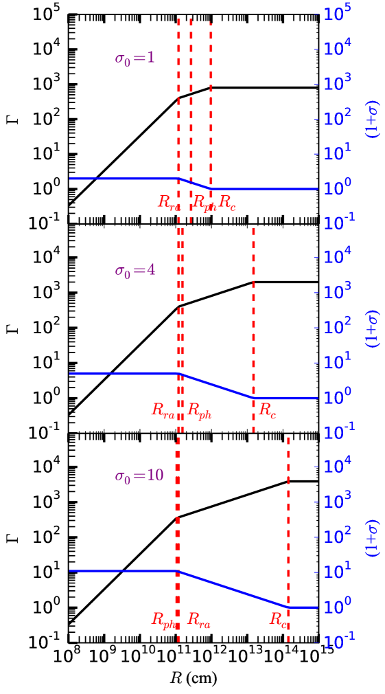
Figure 1: Jet dynamics and some characteristic radii for different magnetization $\sigma_{0}$. The black lines are for $\Gamma$ evolution and the blue lines are for $\sigma$ evolution. Vertical red dashed lines denote three characteristic radii: rapid acceleration radius $R_{\text{ra}}$, photosphere radius $R_{\text{ph}}$, and coasting radius $R_{\text{c}}$. Following parameters are adopted: $L_{w}=10^{53}$ erg s^-1, $R_{0}=3\times 10^{8}$ cm, and $\eta$ $=400$. Different panels correspond to different $\sigma_{0}$: $\sigma_{0}$ $=$ $1$ (top panel), $\sigma_{0}$ $=$ $4$ (middle panel), and $\sigma_{0}$ $=$ $10$ (bottom panel). For the moderate magnetization $\sigma_{0}\simeq 1-10$ considered in this work, $R_{\text{ph}}$ $<$ $R_{\text{c}}$ is satisfied.

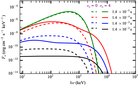
Figure 2: The time-resolved spectra of impulsive injection for the jet with and without magnetization. The solid lines show the calculated time-resolved spectra for the hybrid jet with a hot fireball component ($\eta$ = $400$) and a cold Poynting-flux component ($\sigma_{0}$= $4$). Also, a total outflow luminosity of $L_{w}=10^{53}$ erg s^-1 is assumed, base outflow radius $R_{0}=3\times 10^{8}$ cm, and luminosity distance $d_{\text{L}}=$ $4.85\times 10^{28}$ cm ($z=2$). Different colors represent different observational times. For comparison, the dashed lines illustrate the time-resolved spectra calculated in Deng & Zhang (2014) for the jet without magnetization. Obviously, at later times the time-resolved spectra extend to much higher energy and a power-law component emerges in the low-energy end.

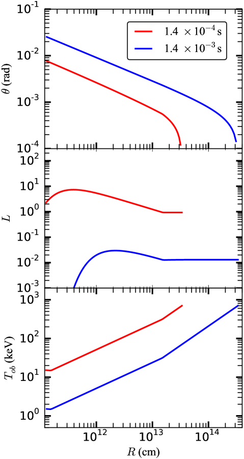
Figure 3: The detailed analysis of the formation of the time-resolved spectra for impulsive injection by illustrating the emitted luminosity and the observer-frame temperature at different positions of the equal arrival time surface. Top panel: the distribution of the angle $\theta$ and the radius $r$ for the equal arrival time surface of different times, $1.4\times 10^{-4}$ s (red) and $1.4\times 10^{-3}$ s (blue). Middle panel: the emitted luminosity in the corresponding radius $r$ for the equal arrival time surface of different times. Bottom panel: the observer-frame temperature in the corresponding radius $r$ for the equal arrival time surface of different times.

The time-resolved spectra of impulsive injection for the hybrid jet are calculated by Equation $(\ref{c})$.  Here we consider a moderate magnetization $\sigma_{0}=$ $4$, since we try to explain the observed spectra with only the thermal component while the non-thermal emission from the Poynting flux is assumed to be weaker. Also, for this scenario the observed relatively large radiative efficiency of the prompt emission $\epsilon_{\gamma}\equiv E_{\gamma}/(E_{\gamma}+E_{k})$ (Lloyd-Ronning & Zhang, 2004; Fan & Piran, 2006; Beniamini et al., 2016) constrains that the kinetic energy powering the afterglow cannot be too large, thus the magnetization $\sigma_{0}$ cannot be too large (for further discussion see section 4.2). Here we do not consider the magnetic dissipation. The magnetic dissipation efficiency depends on the final $\sigma$ after the dissipation (Deng et al., 2015). Then, since the observed prompt luminosity is mainly contributed by the thermal component, which is typically $\sim$ $10^{52}$ erg s^-1, we assume the total outflow luminosity to be $L_{w}=10^{53}$ erg s^-1. As for the base outflow radius $R_{0}$, we take $R_{0}=3\times 10^{8}$ cm close to the mean value of $10^{8.5}$ cm deduced in Pe’er et al. (2015). The luminosity distance is assumed to be $d_{\text{L}}=$ $4.85\times 10^{28}$ cm, according to the peak of the GRB formation rate ($z=2$; see Pescalli et al. 2016). Thus, considering the redshift effect, to obtain the observed typical peak energy $E_{\text{p}}\sim 300$ keV we take the dimensionless entropy $\eta$ $=$ $400$.

The calculated time-resolved spectra with the above parameters are shown in Figure 2 (the solid lines). Also, to illustrate the influence of the magnetization, the time-resolved spectra calculated in Deng & Zhang (2014) for the jet without magnetization are shown with the dashed lines. It is found that at the later times (the high-latitude emission dominates) the time-resolved spectra firstly show a power-law shape extending to a much higher energy than the early-time blackbody. Then, the power-law component vanishes gradually towards the low-energy end and the peak energy on the high-energy end remains constant. To better understanding the formation of the time-resolved spectra, in Figure 3 we show the distribution of the emitted luminosity and the observer-frame temperature at different equal arrival time surfaces (red lines for $1.4\times 10^{-4}$ s, and blue lines for $1.4\times 10^{-3}$ s). For the emitted luminosity, we assume the number of injected photon as $1$.

The emitted luminosity $L$ in the corresponding radius $r$ (with a corresponding angle $\theta$, see the top panel) is shown in the middle panel. While the calculation of this emitted luminosity $L$ is

$$L = \iint P_{1}(r,\mu)\delta(t-\frac{ru}{\beta c})d\mu dr$$ (9)

$$= \iint\text{ }D^{2}\frac{R_{\text{ph}}}{4r^{2}}\left\{\frac{3}{2}+\frac{1}{\pi}\arctan[\frac{1}{3}(\frac{R_{\text{ph}}}{r}-\frac{r}{R_{\text{ph}}})]\right\}$$

$$\times\exp\left[-\frac{R_{\text{ph}}}{6r}(3+\frac{1-\mu^{\prime}}{1+\mu^{\prime}})\right]\times\delta(t-\frac{r(1-\beta\mu)}{\beta c})d\mu dr$$

$$= \int[\Gamma(\frac{\beta ct}{r})]^{-2}\times\frac{R_{\text{ph}}}{4r^{2}}\left\{\frac{3}{2}+\frac{1}{\pi}\arctan[\frac{1}{3}(\frac{R_{\text{ph}}}{r}-\frac{r}{R_{\text{ph}}})]\right\}$$

$$\times\exp\left[-\frac{R_{\text{ph}}}{6r}(3+\frac{1-\mu^{\prime}}{1+\mu^{\prime}})\right]\times\frac{c}{r}dr\text{.}$$

For $r>R_{\text{ph}}$, we have

$$L \simeq [\Gamma(\frac{\beta ct}{r})]^{-2}\times\frac{R_{\text{ph}}}{4r^{2}}\times c$$ (10)

$$\simeq [\Gamma\beta ct]^{-2}\times\frac{R_{\text{ph}}}{4}\times c$$

$$\propto \Gamma^{-2}.$$

Since the jet is still accelerated by the magnetic component as $\Gamma\propto$ $r^{1/3}$ before the coasting radius $R_{c}$, for $R_{\text{ph}}$ $<r<R_{c}$ (see Figure 1) we obtain

$$L\propto r^{-2/3}.$$ (11)

This correlation results in the power-law segment with a slope $\sim-2/3$ (both for $1.4\times 10^{-4}$ s and $1.4\times 10^{-3}$ s) in the middle panel of Figure 3.

As for the observer-frame temperature $T^{\text{ob}}$, considering that the comoving temperature $T^{\prime}(r)$ is constant for $R_{\text{ph}}$ $<r<R_{c}$, we have

$$T^{\text{ob}} \equiv D\cdot T^{\prime}(r)$$ (12)

$$= [\Gamma(r)\cdot(\frac{\beta ct}{r})]^{-1}\cdot T^{\prime}(r)$$

$$\propto r^{2/3}.$$

Thus, a power-law component with a slope $\sim-1$ ($L\propto(T^{\text{ob}})^{-1}$, corresponding to $R_{\text{ph}}$ $<r<R_{c}$) shows up, for the time-resolved spectra at the later times in Figure 2. Also, the peak energy on the high-energy end for these spectra corresponds to the observer-frame temperature at the line of sight ($\theta=0$) and the maximum radius $R_{\max}=\beta ct/(1-\beta)$, namely, $T^{\text{ob}}=\Gamma(R_{\max})\cdot T^{\prime}(R_{\max})$. Since $R_{\max}>R_{\text{ph}}$, the peak energy is surely much higher than that of the early-time blackbody as shown in Figure 2, due to the larger $\Gamma(R_{\max})$ and the constant $T^{\prime}(R_{\max})$. For the much later times, with $R_{\max}>R_{c}$, the peak energy remains unchanged because of the constant $\Gamma(R_{\max})$.

3.2 Continuous Wind

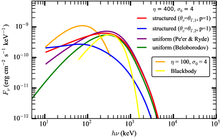
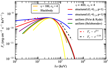
Figure 4: The time-resolved spectra at later times ($t$ $\geq$ $1$ s) of a continuous wind for the hybrid jet with magnetization $\sigma_{0}$= $4$ and various values or angular profiles of dimensionless entropy $\eta$. Left panel: the calculated actual time-resolved spectra. Here, $\theta_{\Gamma,1}=1/400$ and $\theta_{\Gamma,2}=1/4000$. Right panel: the time-resolved spectra which have been normalized to the same peak energy and peak flux as the case of $\eta$ = $400$ and $\sigma_{0}$= $4$ (green line) to compare clearly the low-energy and high-energy indices. For comparison, the yellow lines in the left and right panels show the spectrum of blackbody. Also, the red and black dashed lines in the right panel represent respectively the average low-energy index ($-0.6$) and high-energy index ($-3.24$) fitted with the Band function for the time-resolved spectra of a large sample of single pulses in Yu et al. (2019).

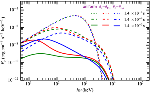
Figure 5: Comparison of the time-resolved spectra of impulsive injection for the hybrid jet with different angular profiles of dimensionless entropy $\eta$. The green lines are the time-resolved spectra in Figure 2 for a uniform profile. While the red and blue lines show the time-resolved spectra for the angular profile with an inner constant core (width of the core $\theta_{c}=\theta_{\Gamma,1}$ for the red lines and $\theta_{c}=\theta_{\Gamma,2}$ for the blue lines) and outer power-law decreased component (power-law index $p=1$). Also, the dashed and solid lines are for the time-resolved spectra at $1.4\times 10^{-4}$ s and $1.4\times 10^{-3}$ s, respectively.

Figure 6: Comparison of the calculated time-resolved spectra at later times ($t$ $\geq$ $1$ s) of a continuous wind with different probability density functions. The parameters of the jet are the same as those used in Deng & Zhang (2014). The three dashed lines show the spectra (normalized to the same peak energy and peak flux as the calculated spectra) of the cutoff power-law model with the low-energy photon index of $0$ (red), $0.3$ (green) and $0.5$ (blue), respectively.

For the continuous wind with constant wind luminosity, the spectrum at a later time ($t$ $\geq$ $1$ s) which corresponds to the observed peak-flux spectrum is calculated by Equation $(\ref{e})$. This calculated time-resolved spectrum, with the same parameters as Figure $2$ ($\eta$ = $400$, $\sigma_{0}$= $4$) is illustrated by the green lines (with the probability density function introduced in Beloborodov 2011) in Figure $4$. Apparently, the spectrum on the high-energy end is a power law rather than an exponential cutoff, which is the natural result of the power-law component extending to much higher energy in Figure $2$. The purple lines are calculated by the probability density function described in Pe’er & Ryde (2011). Also, the spectrum for a smaller dimensionless entropy $\eta$ ($\eta$ = $100$) is shown by the orange line in Figure $4$, which is found to have a smaller peak energy (see the left panel). This is consistent with the positive correlation $T^{\text{ob}}\propto\eta^{16/15}$ in Equation (25) of Gao & Zhang (2015) for the regime of $\eta>(1+\sigma_{0})^{1/2}$ and $R_{\text{ra}}<R_{\text{ph}}<R_{c}$, the regime mainly considered in our work. It is worth noting that, the peak energy weakly depends on the other parameters, i.e., $\sigma_{0}$, $L_{w}$ and $R_{0}$.

Furthermore, we calculate the spectrum (with the probability density function described in Pe’er & Ryde 2011) for the case of the dimensionless entropy $\eta$ of a lateral structure, with which the observed typical low-energy spectral index $\alpha\approx-1$ can be obtained for the unmagnetized jet under the framework of the probability photosphere model (Lundman et al., 2013; Meng et al., 2019). The considered angular Lorentz factor profile consists of an inner constant core with width $\theta_{c}$ and the outer power-law decreased component with power-law index $p$. Note that an angle-independent luminosity is considered, because the spectrum expected to be observed is formed by the photons making their last scattering at approximately $\lesssim 5/$ $\Gamma_{0}$ (as shown in Lundman et al. 2013) and the isotropic angular width for Lorentz factor $\theta_{c,\Gamma}$ is likely to be much smaller than the isotropic angular width for luminosity $\theta_{c,L}$ (see the top panels of Figures 8 and 9 in Zhang,Woosley & MacFadyen 2003, see also section 4.3 for more discussion). The red lines in Figure $4$ represent the calculated spectrum for a hybrid jet with $\theta_{c}=\theta_{\Gamma,1}=1/400$ and $p=1$, corresponding to the typical value $\alpha\sim-1$ for an unmagnetized jet. While the blue lines are the spectrum for hybrid jet with $\theta_{c}=\theta_{\Gamma,2}=1/4000$ and $p=1$, corresponding to the minimum value $\alpha\sim-2$ for unmagnetized jet (see Figure 7d in Meng et al. 2019). To compare clearly the low-energy and high-energy indices, in Figure $4$ the calculated actual time-resolved spectra (left panel) have been normalized to the same peak energy and peak flux as the case of $\eta$ = $400$ and $\sigma_{0}$= $4$ (shown in the right panel).

We then find that the spectrum of the hybrid jet possesses the much harder low-energy spectral index than that of the unmagnetized jet with the same angular profile, $\alpha\sim-0.6$ for $\theta_{c}=\theta_{\Gamma,1}$, $p=1$ and $\alpha\sim-1$ for $\theta_{c}=\theta_{\Gamma,2}$, $p=1$. To better understand the origin of this hardness, in Figure $5$ we show the time-resolved spectra of impulsive injection for these two angular profiles. The power-law segment caused by the magnetic acceleration, similar to that for the uniform profile in Figure $2$ and noteworthily with the swallower slope ($\sim-1$) than that of the power law ($\sim-2$) for the unmagnetized structured jet (Meng et al., 2019), exists close to and below the peak energy of the early-time blackbody in the late-time spectra. This results in the above hardness for the spectrum of continuous wind. On the high-energy end, with the angular profile of the dimensionless entropy, the spectrum remains to be a power law. The high-energy power-law index $\beta$ is the same as the uniform case for $\theta_{c}=\theta_{\Gamma,1}$, $p=1$ ($\beta\sim-4$, see Figure $9$ and the discussion in Section $3.3$), and much larger ($\beta\sim-1.6$) for $\theta_{c}=\theta_{\Gamma,2}$, $p=1$. In a word, the spectrum of the hybrid jet is analogue to the empirical Band function (Band et al., 1993) spectrum, whereas the spectrum of the unmagnetized jet corresponds to the spectrum of the empirical cutoff power-law model (Meng et al., 2019), within the framework of the probability photosphere model.

Interestingly, in all the statistical works of a large sample of GRBs (e.g. Kaneko et al., 2006; Goldstein et al., 2012, 2013; Gruber et al., 2014; Yu et al., 2016), the average low-energy spectral index for the GRBs best-fitted by the Band function is harder ($0.1\sim 0.3$) than that for the GRBs best-fitted by the cutoff power-law model, for both the time-integrated and the peak-flux spectra. This hardness is quite consistent with our results for the probability photosphere model discussed in the previous paragraph. Also, for the distributions of the low-energy and high-energy indices, our results (corresponding to the peak-flux spectra) are quite similar to the statistical results of the peak-flux spectra for the GRBs best-fitted by the Band function. For the low-energy spectral index, the typical value is $\alpha\sim-0.6$ and the minimum value $\alpha\sim-1$. While for the high-energy spectral index, the maximum value $\beta\sim-1.6$ in our model is close to the statistical result. The typical value $\beta\sim-4$ in our model seems to be much softer than the well-known $\beta\sim-2.5$, which we consider to arise from the assumption of the single pulse, namely without the overlap of the pulses. This consideration is proposed recently in Yu et al. (2019), where the time-resolved spectral analysis of a large sample of single pulses has been performed and the average high-energy spectral index ($\beta\sim-3.24$) indeed is found to be much softer. Noteworthily, the average high-energy spectral index $\beta\sim-3.24$ in that work can be well reproduced with our hybrid jet model, by considering the parameter dependence on the power-law index of magnetic acceleration $\delta$ (see Figure $9$ and the discussion in Section $3.3$). In the right panel of Figure $4$, the red and black dashed lines represent the average low-energy index ($-0.6$) and high-energy index ($-3.24$) in that work, respectively.

In the following, we give a detailed discussion on the maximum (or the hardest) low-energy spectral index $\alpha$. The maximum $\alpha$ from the statistical works is $\alpha\sim 0$, for the GRBs best-fitted by the Band function and the cutoff power-law model both. For the probability photosphere model, with magnetization or not, the maximum $\alpha$ corresponds to a uniform jet. The low-energy index $\alpha$ of the calculated spectrum for a uniform jet is regarded as $\alpha\sim 0.5$ in Deng & Zhang (2014), while $\alpha\sim 0$ is obtained in Lundman et al. (2013) (see the high-energy inner jet spectral component for a wide jet $\theta_{\text{j}}=10/\Gamma_{0}$ and $\theta_{\text{v}}=0$ in Figure $8$, the red diamonds and solid black lines) and Meng et al. (2019) (see Figure $7b$ therein). We notice that, in Deng & Zhang (2014) (see Figure $3$ and Figure $9$) $\alpha\sim 0.5$ is taken from the power-law index close to $3$ keV. But this is quite rough, since the actual power-law index is determined by the fitting of the observed spectrum from $8$ keV to the peak energy $\sim$ $300$ keV, quite above $3$ keV. Thus, in Figure $6$ we compare the calculated spectra in Deng & Zhang (2014) (orange and magenta lines) with the spectra of the cutoff power-law model for $\alpha=$ $0$, $\alpha=0.3$ and $\alpha=0.5$. The orange line is calculated by the probability density function introduced in Beloborodov (2011), while the magenta line is for the probability density function proposed in Deng & Zhang (2014). Notice that, the spectra of the cutoff power-law model have been normalized to the same peak energy and peak flux as the calculated spectra. In Figure $6$, we also plot the calculated spectra with the probability density function described in Pe’er & Ryde (2011) and Lundman et al. (2013), using the same jet parameters as those in Deng & Zhang (2014). It is found that, except for the probability density function in Beloborodov (2011), the calculated spectra for the other three kinds of probability density function are similar, all close to the cutoff power-law spectrum for $\alpha=$ $0$ from $\sim$ $20$ keV to the peak energy $\sim$ $300$ keV. This is consistent with the maximum $\alpha$ from the statistical works. While the calculated spectrum for the probability density function in Beloborodov (2011) is quite close to the cutoff power-law spectrum for $\alpha=$ $0.3$. We think two aspects are responsible for this hardness: the angle corresponding to the observer-frame temperature of $\sim$ $8$ keV to $\sim$ $300$ keV is small ($\lesssim 5/\Gamma_{0}$, also see the top and bottom panels in Figure $3$); and the probability density function for the small angle in Beloborodov (2011) is not as good as the others (see the solid lines in Figure 7 of Deng & Zhang 2014).

3.3 Parameter Dependence

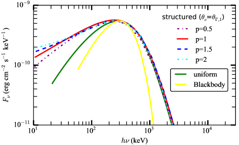
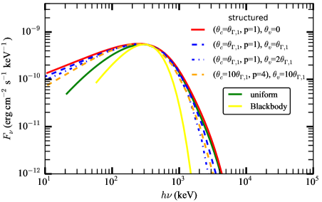
Figure 7: The calculated time-resolved spectra at later times ($t$ $\geq$ $1$ s) of continuous wind for a structural angular profiles of dimensionless entropy $\eta$ with different power-law index $p$ or non-zero viewing angle. Left panel: the dependence of the time-resolved spectra on the power-law index, $p=1$ (red solid), $p=0.5$ (magenta dash-dotted), $p=1.5$ (blue dashed) and $p=2$ (cyan dash-dotted). Right panel: the time-resolved spectra with non-zero viewing angle. The dashed and dash-dotted lines are for $\theta_{v}=\theta_{\Gamma,1}$ and $\theta_{v}=2\cdot\theta_{\Gamma,1}$ respectively, along with $\theta_{c}=\theta_{\Gamma,1}$ and $p=1$. While the orange dashed line is for $\theta_{v}=10\cdot\theta_{\Gamma,1}$ with $\theta_{c}=10\cdot\theta_{\Gamma,1}$ and $p=4$. The green and yellow lines are the same as those in Figure 4.

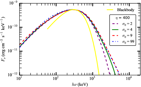
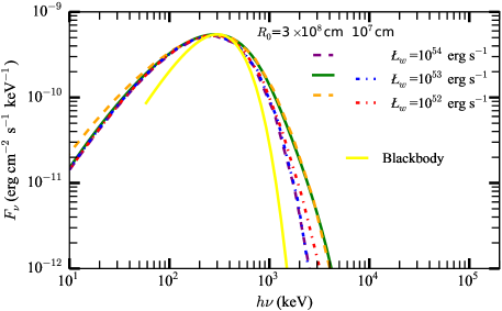
Figure 8: The calculated time-resolved spectra at later times ($t$ $\geq$ $1$ s) of continuous wind with different magnetization $\sigma_{0}$ or combination of $L_{w}$ and $R_{0}$. Left panel: the dependence of the time-resolved spectra on the magnetization, $\sigma_{0}=2$ (purple dashed), $\sigma_{0}=9$ (red dashed) and $\sigma_{0}=99$ (blue dash-dotted). Right panel: the time-resolved spectra with different combination of $L_{w}$ and $R_{0}$. The purple and orange dashed lines are for $L_{w}=10^{54}$ erg s^-1 and $L_{w}=10^{52}$ erg s^-1 respectively, along with $R_{0}=3\times 10^{8}$ cm. While the blue and red dash-dotted lines are for $L_{w}=10^{53}$ erg s^-1 and $L_{w}=10^{52}$ erg s^-1 respectively, along with $R_{0}=10^{7}$ cm. The green and yellow lines are also the same as those in Figure 4.

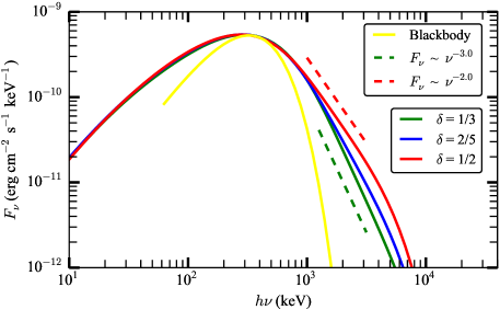
Figure 9: The calculated time-resolved spectra at later times ($t$ $\geq$ $1$ s) of continuous wind with different power-law index of magnetic acceleration $\delta$. The green, blue and red lines are for $\delta=1/3$, $\delta=2/5$ and $\delta=1/2$ respectively, along with magnetization $\sigma_{0}=9$. While the green and red dashed lines represent the high-energy spectral index $\beta=-4$ and $\beta=-3$, respectively. The yellow line is the spectrum of blackbody.

As shown in Figure 4, the calculated spectrum of continuous wind for our hybrid jet model can reproduce the observed low-energy and high-energy indices quite well, for the GRBs best-fitted by the Band function. In this section, we analyze in detail the dependence of these spectral indices on the power-law index of the dimensionless entropy profile $p$ and the viewing angle $\theta_{v}$ (Figure 7), the magnetization $\sigma_{0}$ and the combination of $L_{w}$ and $R_{0}$ (Figure 8), and the power-law index of magnetic acceleration $\delta$ (Figure 9). In Figures 7-9, all the calculated spectra have been normalized to the same peak energy and peak flux as the case of $\eta$ = $400$ and $\sigma_{0}$= $4$ (green line).

From the left panel of Figure 7 we can see that, with $\theta_{c}=1/400$ and different values of $p$, the high-energy spectrum is almost the same and the low-energy spectral index does not change a lot. The low-energy spectral index is slightly softer for $p=1.5$ and $p=2$, while slightly harder for $p=0.5$. Also, the influence of non-zero viewing angle on the spectrum is shown in the right panel of Figure 7. With a non-zero viewing angle $\theta_{v}=\theta_{\Gamma,1}$ or $\theta_{v}=2\cdot\theta_{\Gamma,1}$ the spectrum becomes narrower, namely, the low-energy spectrum is harder and the high-energy spectrum deviates a little from the power law to the exponential cutoff. This is consistent with the spectral result of smaller $\eta$ (see the orange line in the right panel of Figure 4) and quite different from the unmagnetized case, in which the shape of the spectrum remains unchanged with a non-zero viewing angle. In addition, the low-energy spectral index for $\theta_{c}=10\cdot\theta_{\Gamma,1}$, $p=1$ and $\theta_{v}=10\cdot\theta_{\Gamma,1}$ is found to be much harder than that of the unmagnetized case ($\alpha$ $\sim$ $-1$), just as the situation for $\theta_{c}=\theta_{\Gamma,1}$, $p=1$ mentioned above.

The dependence of the shape of the calculated spectrum on the magnetization $\sigma_{0}$ is illustrated in the left panel of Figure 8. Notice that we take the total luminosity $L_{w}=6\times 10^{52}$ erg s^-1 for $\sigma_{0}=2$, to have comparable prompt emission luminosity with the case of $\sigma_{0}=4$. And we keep $L_{w}=10^{53}$ erg s^-1 for $\sigma_{0}=9$ and the extreme case of $\sigma_{0}=99$, to account for the $R_{\text{ph}}<R_{\text{ra}}$ regime. With smaller magnetization $\sigma_{0}$ ($\sigma_{0}=2$), the spectrum is narrower in both the low-energy (slightly) and high-energy (significantly) ends. If the magnetization is larger ($\sigma_{0}=9$ or even $\sigma_{0}=99$), entering the $R_{\text{ph}}<R_{\text{ra}}$ regime, the low-energy spectrum is a little softer and the high-energy power law can extend to much higher energy with the approximate slope as the $\sigma_{0}=4$ case. This softness and higher energy is due to the larger range of $R_{\text{ph}}$ $<r<R_{c}$, which is responsible for the high-energy power law with negative index (see Figure 3 and the discussion there).

In the right panel of Figure 8, we plot the calculated spectra for different combinations of $L_{w}$ and $R_{0}$. The low-energy spectrum is almost the same except for the case of $L_{w}=10^{52}$ erg s^-1 and $R_{0}=3\times 10^{8}$ cm, which enters the $R_{\text{ph}}<R_{\text{ra}}$ regime and thus has the slightly softer low-energy spectrum. The shape of the high-energy spectrum depends on the comparison of $R_{\text{ph}}$ and $R_{\text{ra}}$. For $L_{w}=10^{52}$ erg s^-1 and $R_{0}=3\times 10^{8}$ cm, the high-energy spectrum is close to the reference spectrum. For the other three combinations, since $R_{\text{ph}}$ is much greater than $R_{\text{ra}}$, the high-energy spectrum becomes narrower.

Note that in the above discussion, for the magnetically driven acceleration, we only consider the case of magnetic reconnection for the non-axisymmetric rotator (Drenkhahn, 2002; Drenkhahn & Spruit, 2002). Whereas, for an initially axisymmetric flow, the acceleration can happen through the kink instability (Lyutikov & Blandford, 2003; Giannios & Spruit, 2006). Besides, the magnetic acceleration driven by the kink instability seems to be more rapid than the magnetic reconnection case, with a larger power-law index $\delta$ of $\sim 2/5$ or even $\sim 1/2$ (see Figure 5 in Giannios & Spruit 2006). Thus, in Figure 9 we compare the calculated spectra of our model for $\delta=1/3$, $\delta=2/5$ and $\delta=1/2$, and find that their high-energy power-law indices are quite different while the low-energy indices remain the same. For $\delta=1/3$, we have $\beta=-4$; for $\delta=1/2$, we obtain $\beta=-3$; and $\beta$ lies between $-4$ and $-3$ for $\delta=2/5$. Surprisingly, this rough distribution of $\beta$ ($-4$ to $-3$) is well consistent with the $\beta$ distribution of the softer cluster for a large sample of single pulses in Yu et al. (2019), where the $\beta$ distribution seems to show the bimodal distribution with a harder typical cluster (peaks at $-2.5$) and a softer cluster (peaks at $-3.5$; see Figure 1 therein).

4 Discussion

4.1 Magnetic Dissipation

Significant magnetic dissipation may happen below the photosphere according to several previous works (e.g. Thompson, 1994; Rees & Mészáros, 2005; Giannios, 2008; Mészáros & Rees, 2011; Veres & Mészáros, 2012), thus enhancing the photosphere emission. However, in this sub-photosphere region complete thermalization may not be achieved due to the lack of enough photons (low creation rate), for the case of Poynting-flux-dominated outflow. Then, the photosphere spectrum could have a non-thermal shape with an ultra-high peak energy $E_{p}$ ranging from 1 MeV to about 20 MeV (Giannios, 2006; Beloborodov, 2013; Bégué & Pe’er, 2015). But we think that, for the hybrid jet with moderate magnetization considered in this work, complete thermalization may be achieved because of the existence of the extra thermal component in the outflow. Thus, the spectrum emitted at a particular position could be a blackbody with the temperature a bit larger than the non-dissipative case (see Equation (30) in Gao & Zhang 2015). The shape of the observed overall spectrum is still the same as that for the non-dissipative case.

4.2 Radiative Efficiency

The radiative efficiency of the prompt emission $\epsilon_{\gamma}$, generally defined as $E_{\gamma}/(E_{\gamma}+E_{k})$, is a crucial quantity to distinguish different prompt emission models. Here, $E_{\gamma}$ means the radiated energy in the prompt phase and $E_{k}$ means the remaining kinetic energy in the afterglow phase. For the photosphere emission model of a hybrid jet with moderate magnetization considered in this work, we have

$$\epsilon_{\gamma} = \frac{E_{\gamma}}{E_{\gamma}+E_{k}}$$ (13)

$$= \frac{L_{\text{Th}}\times(R_{\text{ph}}/R_{\text{ra}})^{-7/9}}{L_{\text{Th}}+L_{P}}$$

$$= \frac{(R_{\text{ph}}/R_{\text{ra}})^{-7/9}}{1+\sigma_{0}}\text{,}$$

in the typical $R_{\text{ph}}\geq R_{\text{ra}}$ regime. While, $\epsilon_{\gamma}=1/(1+\sigma_{0})$ is obtained in the $R_{\text{ph}}\leq R_{\text{ra}}$ regime. Note that the magnetic energy is thought to be transferred to the kinetic energy completely before the onset of the afterglow, because of the moderate magnetization. Then, for $\sigma_{0}\sim 2-9$ considered above, $\epsilon_{\gamma}$ ranges from a few percents to $\sim 0.3$. Namely, our photosphere model predicts a relatively low efficiency of $\sim 0.1$.

Observationally, $E_{k}$ can be inferred through the late-time X-ray afterglow (Kumar, 2000; Freedman & Waxman, 2001). Then, along with the obtained $E_{\gamma}$ by integrating the prompt spectrum, the radiative efficiency $\epsilon_{\gamma}$ can be obtained. The inferred radiative efficiency is quite high, $\epsilon_{\gamma}\sim$ $0.4$ $-1.0$, in most of previous studies (Lloyd-Ronning & Zhang, 2004; Berger, 2007; Nysewander et al., 2009; D’Avanzo et al., 2012; Wygoda et al., 2016). This favors greatly the photosphere emission model without magnetization, especially with larger $R_{0}$ inferred in Pe’er et al. (2015) since $R_{\text{ph}}$ is more close to saturation radius $R_{\text{s}}$. Note that the above method considers that the late-time X-ray afterglow is contributed by fast cooling electrons (for the typical values of magnetic equipartition parameter $\epsilon_{B}\simeq 0.01-0.1$) . If $\epsilon_{B}$ is smaller ( $\sim 10^{-4}$) for a portion of GRBs as inferred in several works (Barniol Duran, 2014; Santana et al., 2014; Wang et al., 2015; Zhang et al., 2015), slow cooling or significant Inverse Compton losses take place and the estimated radiative efficiency $\epsilon_{\gamma}\sim 0.1$ is smaller (Fan & Piran, 2006; Beniamini et al., 2016). This portion of GRBs may correspond to the photosphere emission with moderate magnetization discussed in this work.

4.3 Availability of the Assumption of $\theta_{c,\Gamma}<\theta_{c,L}$

As stated above, since the observed spectrum is contributed by the photons emitted from a rather narrow angular region ($\lesssim 5/$ $\Gamma_{0}$) and $\theta_{c,\Gamma}<\theta_{c,L}$ is likely to be the real situation based on the simulation, we take $dL/d\Omega\approx$ const in our calculations. Namely, we only consider the case of smaller viewing angle ($\theta_{v}<\theta_{c,L}$). The assumption of $\theta_{c,\Gamma}<\theta_{c,L}$ is supported in some prior simulations, including both hydrodynamical ones (Lazzati et al., 2007; Ito et al., 2021) and magnetohydrodynamical ones (MHD, Tchekhovskoy et al. 2008; Geng et al. 2019).

Theoretically, $\theta_{c,\Gamma}<\theta_{c,L}$ could be understood as a natural result of the enhanced material density for larger angle (see Figure 3 in Lazzati et al. 2007). The structured jet is produced because the jet will be collimated by the progenitor envelope (or dynamical ejecta) when penetrating it. This progenitor envelope (or dynamical ejecta) is matter-dominated, and makes the shocked jet have an increased material density (for larger angle) when collimation happens. Then, since $\Gamma(\theta)\propto L/M(\theta)$, the Lorentz factor will start to decrease even when the $L$ remains constant. Namely, $\theta_{c,\Gamma}<\theta_{c,L}$ is obtained.

However, due to the complexity of simulations and lack of robust results, $\theta_{c,\Gamma}$ $>$ $\theta_{c,L}$ may also be common in realistic situations. Here, in Figure 10 we also perform calculations for the case of $\theta_{c,\Gamma}=\theta_{c,L}$, which is often adopted for structured jet in the literature. The other parameters are the same as those in Figure 4. Besides, $\theta_{c,L}=\theta_{c,\Gamma}=1/400$, and q is the power-law decreased index for luminosity. In this case, the low-energy spectral index $\alpha$ is much harder. This is because the low-energy photons emitted from the high-latitude region become much less (since the luminosity is smaller). Then, the observed bursts with harder low-energy spectral index can be reproduced in this case. Furthermore, according to recent studies (Meng et al., 2018; Burgess et al., 2020) $\alpha$ may not be a good indicator to justify the radiation mechanism, we should use the model spectrum to directly fit the data.

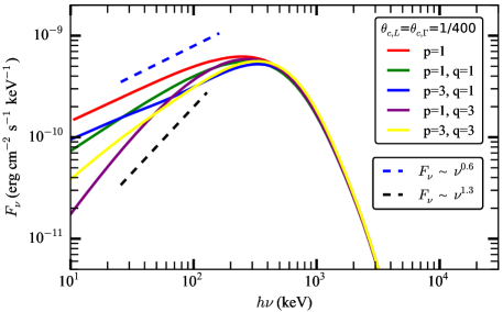
Figure 10: The time-resolved spectra at later times ($t$ $\geq$ $1$ s) of a continuous wind for structured jet with $\theta_{c,L}=\theta_{c,\Gamma}=1/400$ and various power-law decreased indices of luminosity (q) and Lorentz factor (p). A hybrid jet with magnetization $\sigma_{0}$ = $4$ is considered, and the Lorentz factor in the isotropic core is $400$. The red line is the same as that in Figure 4, for an angle-independent luminosity ($\alpha\sim-0.6$). Obviously, for the combinations of p=1 and q=1 (the green line) and of p=3 and q=1 (the blue line), the low-energy spectral index $\alpha$ is only slightly harder than that of the angle-independent luminosity case. While for the combinations of p=1 and q=3 (the purple line) and of p=3 and q=3 (the yellow line), the low-energy spectral index $\alpha$ is much harder. The blue and black dashed lines represent the low-energy spectral indices of $-0.4$ ($F_{\nu}\sim\nu^{0.6}$) and $0.3$ ($F_{\nu}\sim\nu^{1.3}$), respectively.

4.4 Impact on the observed spectra by the synchrotron emission

Synchrotron emission may also contribute to the observed spectrum for a hybrid jet. Considering the synchrotron emission from magnetic dissipation, the high-energy spectrum may be less steeper when peak energy of the photosphere spectrum is comparable with that of the synchrotron spectrum. Otherwise, a two-peak spectrum is likely to exist. For smaller $\sigma_{0}$, the photosphere component may dominant, while synchrotron component may dominant for larger $\sigma_{0}$.

5 CONCLUSIONS

In this paper, by invoking the probability photosphere model we investigate the shape of the photospheric emission spectrum for the hybrid outflow, which contains a thermal component and a magnetic component with moderate magnetization ($\sigma_{0}=L_{P}/L_{\text{Th}}\sim 1-10$). The following conclusions are drawn.

(1) The photosphere spectrum on the high-energy end is a power law rather than an exponential cutoff. This high-energy power-law component arises from the continued increase of the bulk Lorentz factor $\Gamma$ (due to the magnetically driven acceleration of the magnetic component) and the constant comoving temperature $T^{\prime}$ above the photosphere radius $R_{\text{ph}}$, where the emission is not negligible (though less) according to the probability photosphere model. The power-law segment can extend to higher energy with larger magnetization $\sigma_{0}$ (smaller $L_{w}$, larger $R_{0}$, or larger $\eta$), because of the larger range of $R_{\text{ph}}$ $<r<R_{c}$ (responsible for the high-energy power law).

(2) With the similar angular profiles of the dimensionless entropy $\eta$ as the unmagnetized jet, considered in previous works (Lundman et al., 2013; Meng et al., 2019), the distribution of the low-energy indices (corresponding to the peak-flux spectra) for our photosphere model is quite consistent with the statistical result of the peak-flux spectra for the GRBs best-fitted by the Band function. For a combination of $\theta_{c}=1/\Gamma=1/400$ and $p=1$, with the unmagnetized probability photosphere model, the resulted $\alpha$ is consistent with the observed typical value $\alpha\sim-1.0$ for the GRBs best-fitted by the cutoff power law. Considering the magnetized probability photosphere model in this work, the obtained $\alpha$ is accordant with the observed typical value $\alpha\sim-0.6$ for the GRBs best-fitted by the Band function. While for a combination of an extremely narrow core $\theta_{c}=1/(10\Gamma)=1/4000$ and $p=1$, with the unmagnetized probability photosphere model, the resulted $\alpha$ is consistent with the observed minimum value $\alpha\sim-2.0$ for the GRBs best-fitted by the cutoff power law. Considering the magnetized probability photosphere model in this work, the obtained $\alpha$ is accordant with the observed minimum value $\alpha\sim-1$ for the GRBs best-fitted by the Band function. Also, by analyzing the low-energy spectra for uniform jet calculated with different probability density functions, we find that the hardest $\alpha$ predicted by the probability photosphere model (both unmagnetized and magnetized) should be $\alpha\sim 0$, almost the same as both the observed maximum values for the GRBs best-fitted by the cutoff power law and the Band function.

(3) The high-energy power-law index $\beta$ for our photosphere model solely depends on the power-law index of magnetic acceleration $\delta$, if only the core for the angular profile of $\eta$ is not too narrow. After considering the magnetic acceleration due to magnetic reconnection for the non-axisymmetric rotator ($\delta\sim 1/3$) and kink instability in an initially axisymmetric flow ($\delta\sim 1/2$), the distribution of the obtained $\beta$ (from $-4$ to $-3$; $\beta=-4$ for $\delta=1/3$, and $\beta=$ $-3$ for $\delta=1/2$) is well consistent with the $\beta$ distribution of the softer cluster for a large sample of single pulses in Yu et al. (2019). Besides, for an extremely narrow core $\theta_{c}=1/(10\Gamma)=1/4000$ and $p=1$, much larger $\beta\sim$ $-1.6$ is obtained, similar to the maximum value of the statistical result. In total, the observed $\beta$ distribution could be well interpreted with the photosphere model in this work.

Data availability

The data underlying this article will be shared on reasonable request to the corresponding author.

References

- Abdo et al. (2009) Abdo A. A., et al., 2009, ApJ, 706, L138
- Abramowicz et al. (1991) Abramowicz M. A., Novikov I. D., Paczynski B., 1991, ApJ, 369, 175
- Acuner & Ryde (2018) Acuner Z., Ryde F., 2018, MNRAS, 475, 1708
- Acuner et al. (2020) Acuner Z., Ryde F., Pe’er A., Mortlock D., Ahlgren B., 2020, ApJ, 893, 128
- Aloy et al. (2005) Aloy M. A., Janka H.-T., Müller E., 2005, A&A, 436, 273
- Axelsson et al. (2012) Axelsson M., et al., 2012, ApJ, 757, L31
- Axelsson & Borgonovo (2015) Axelsson M., Borgonovo L., 2015, MNRAS, 447, 3150
- Band et al. (1993) Band D., et al., 1993, ApJ, 413, 281
- Barniol Duran (2014) Barniol Duran R., 2014, MNRAS, 442, 3147
- Bégué & Pe’er (2015) Bégué D., Pe’er A. 2015, ApJ, 802, 134
- Beloborodov (2011) Beloborodov A. M., 2011, ApJ, 737, 68
- Beloborodov (2013) Beloborodov A. M., 2013, ApJ, 764, 157
- Beloborodov (2017) Beloborodov A. M., 2017, ApJ, 838, 125
- Beniamini et al. (2016) Beniamini P., Nava L., Piran T., 2016, MNRAS, 461, 51
- Berger (2007) Berger E., 2007, ApJ, 670, 1254
- Burgess et al. (2017) Burgess J. M., Greiner J., Bégué D., Berlato F., 2017, arXiv:1710.08362
- Burgess (2019) Burgess J. M., 2019, A&A, 629, A69
- Burgess et al. (2020) Burgess J. M., Bégué D., Greiner J., Giannios D., Bacelj A., Berlato F., 2020, Nature Astronomy, 4, 174
- Dai & Gou (2001) Dai Z. G., Gou L. J., 2001, ApJ, 552, 72
- D’Avanzo et al. (2012) D’Avanzo P., et al., 2012, MNRAS, 425, 506
- Deng & Zhang (2014) Deng W., Zhang B., 2014, ApJ, 785, 112
- Deng et al. (2015) Deng W., Li H., Zhang B., Li S., 2015, ApJ, 805, 163
- Drenkhahn (2002) Drenkhahn G., 2002, A&A, 387, 714
- Drenkhahn & Spruit (2002) Drenkhahn G., Spruit H. C., 2002, A&A, 391, 1141
- Duan, & Wang (2019a) Duan M.-Y., Wang X.-G., 2019, ApJ, 884, 61
- Duan, & Wang (2019b) Duan M.-Y., Wang X.-G., 2020, ApJ, 890, 90
- Fan & Piran (2006) Fan Y.-Z., Piran T., 2006, MNRAS, 369, 197
- Fan et al. (2012) Fan Y.-Z., Wei D.-M., Zhang F.-W., Zhang B.-B., 2012, ApJ, 755, L6
- Ford et al. (1995) Ford L. A., et al., 1995, ApJ, 439, 307
- Freedman & Waxman (2001) Freedman D. L., Waxman E., 2001, ApJ, 547, 922
- Gao & Zhang (2015) Gao H., Zhang B., 2015, ApJ, 801, 103
- Geng et al. (2018) Geng J.-J., Huang Y.-F., Wu X.-F., Zhang B., Zong H.-S., 2018, ApJS, 234, 3
- Geng et al. (2019) Geng J.-J., Zhang B., Kölligan A., Kuiper R., Huang Y.-F., 2019, ApJ, 877, L40
- Ghirlanda et al. (2010) Ghirlanda G., Nava L., Ghisellini G., 2010, A&A, 511, A43
- Ghirlanda et al. (2013) Ghirlanda G., Pescalli A., Ghisellini G., 2013, MNRAS, 432, 3237
- Giannios (2006) Giannios D., 2006, A&A, 457, 763
- Giannios & Spruit (2006) Giannios D., Spruit H. C., 2006, A&A, 450, 887
- Giannios (2008) Giannios D., 2008, A&A, 480, 305
- Goldstein et al. (2012) Goldstein A., et al.,2012, ApJS, 199, 19
- Goldstein et al. (2013) Goldstein A., Preece R. D., Mallozzi R. S., Briggs M. S., Fishman G. J., Kouveliotou C., Paciesas W. S.,Burgess J. M., 2013, ApJS, 208, 21
- Goodman (1986) Goodman J., 1986, ApJ, 308, L47
- Gottlieb et al. (2021) Gottlieb O., Nakar E., Bromberg O., 2021, MNRAS, 500, 3511
- Granot et al. (2011) Granot J., Komissarov S. S., Spitkovsky A., 2011, MNRAS, 411, 1323
- Gruber et al. (2014) Gruber D., et al., 2014, ApJS, 211, 12
- Guiriec et al. (2013) Guiriec S., et al., 2013, ApJ, 770, 32
- Guiriec et al. (2011) Guiriec S., et al., 2011, ApJ, 727, L33
- Hou et al. (2018) Hou S.-J., et al., 2018, ApJ, 866, 13
- Huang et al. (2019) Huang B.-Q., Lin D.-B., Liu T., Ren J., Wang X.-G., Liu H.-B., Liang E.-W., 2019, MNRAS, 487, 3214
- Ito et al. (2021) Ito H., Just O., Takei Y., Nagataki S., 2021, ApJ, 918, 59
- Kaneko et al. (2006) Kaneko Y., Preece R. D., Briggs M. S., Paciesas W. S., Meegan C. A., Band D. L., 2006, ApJS, 166, 298
- Komissarov et al. (2009) Komissarov S. S., Vlahakis N., Königl A., Barkov M. V., 2009, MNRAS, 394, 1182
- Komissarov et al. (2010) Komissarov S. S., Vlahakis N., Königl A., 2010, MNRAS, 407, 17
- Kumar (2000) Kumar P., 2000, ApJ, 538, L125
- Kumar & Granot (2003) Kumar P., Granot J., 2003, ApJ, 591, 1075
- Larsson et al. (2015) Larsson J., Racusin J. L., Burgess J. M., 2015, ApJ, 800, L34
- Lazzati et al. (2007) Lazzati D., Morsony B. J., Begelman M. C., 2007, Philosophical Transactions of the Royal Society of London Series A, 365, 1141
- Lazzati et al. (2013) Lazzati D., Morsony B. J., Margutti R., Begelman M. C., 2013, ApJ, 765, 103
- Lei et al. (2013) Lei W.-H., Zhang B., Liang E.-W., 2013, ApJ, 765, 125
- Li (2019a) Li L., 2019a, ApJS, 242, 16
- Li et al. (2019b) Li L., et al., 2019b, ApJ, 884, 109
- Li (2019c) Li L., 2019c, ApJS, 245, 7
- Li (2019d) Li L., 2020, ApJ, 894, 100
- Liang & Kargatis (1996) Liang E., Kargatis V., 1996, Nature, 381, 49
- Lin et al. (2018) Lin D.-B., Liu T., Lin J., Wang X.-G., Gu W.-M., Liang E.-W., 2018, ApJ, 856, 90
- Lloyd-Ronning & Zhang (2004) Lloyd-Ronning N. M., Zhang B., 2004, ApJ, 613, 477
- Lu et al. (2010) Lu R.-J., Hou S.-J., Liang E.-W., 2010, ApJ, 720, 1146
- Lu et al. (2012) Lu R.-J., Wei J.-J., Liang E.-W., Zhang B.-B., Lü H.-J., Lü L.-Z., Lei W.-H., Zhang B., 2012, ApJ, 756, 112
- Lu et al. (2017) Lu R.-J., Du S.-S., Cheng J.-G., Lü H.-J., Zhang H.-M., Lan L., Liang E.-W., 2017, arXiv:1710.06979
- Lundman et al. (2013) Lundman C., Pe’er A., Ryde F., 2013, MNRAS, 428, 2430
- Lyutikov & Blandford (2003) Lyutikov M., Blandford R., 2003, arXiv:astro-ph/0312347
- MacFadyen & Woosley (1999) MacFadyen A. I., Woosley S. E., 1999, ApJ, 524, 262
- Meng et al. (2018) Meng Y.-Z., et al., 2018, ApJ, 860, 72
- Meng et al. (2019) Meng Y.-Z., Liu L.-D., Wei J.-J., Wu X.-F., Zhang B.-B., 2019, ApJ, 882, 26
- Mészáros & Rees (2000) Mészáros P., Rees M. J., 2000, ApJ, 530, 292
- Mészáros (2002) Mészáros P., 2002, ARA&A, 40, 137
- Mészáros & Rees (2011) Mészáros P., Rees M. J., 2011, ApJ, 733, L40
- Metzger et al. (2011) Metzger B. D., Giannios D., Thompson T. A., Bucciantini N., Quataert E., 2011, MNRAS, 413, 2031
- Mizuta, Nagataki & Aoi (2011) Mizuta A., Nagataki S., Aoi J., 2011, ApJ, 732, 26
- Morsony, Lazzati & Begelman (2007) Morsony B. J., Lazzati D., Begelman M. C., 2007, ApJ, 665, 569
- Murguia-Berthier et al. (2017) Murguia-Berthier A., et al., 2017, ApJL, 835, L34
- Nagakura et al. (2011) Nagakura H., Ito H., Kiuchi K., Yamada S., 2011, ApJ, 731, 80
- Nysewander et al. (2009) Nysewander M., Fruchter A. S., Pe’er A., 2009, ApJ, 701, 824
- Paczynski (1986) Paczynski B., 1986, ApJ, 308, L43
- Pe’er (2008) Pe’er A., 2008, ApJ, 682, 463
- Pe’er & Ryde (2011) Pe’er A., Ryde F., 2011, ApJ, 732, 49
- Pe’er et al. (2015) Pe’er A., Barlow H., O’Mahony S., Margutti R., Ryde F., Larsson J., Lazzati D., Livio M., 2015, ApJ, 813, 127
- Pescalli et al. (2016) Pescalli A., et al., 2016, A&A, 587, A40
- Piran et al. (1993) Piran T., Shemi A., Narayan R., 1993, MNRAS, 263, 861
- Piran (1999) Piran T., 1999, Phys. Rep., 314, 575
- Preece et al. (2000) Preece R. D., Briggs M. S., Mallozzi R. S., Pendleton G. N., Paciesas W. S., Band D. L., 2000, ApJS, 126, 19
- Rees & Meszaros (1994) Rees M. J., Meszaros, P., 1994, ApJ, 430, L93
- Rees & Mészáros (2005) Rees M. J., Mészáros P., 2005, ApJ, 628, 847
- Rossi et al. (2002) Rossi E., Lazzati D., Rees M. J., 2002, MNRAS, 332, 945
- Rosswog (2013) Rosswog S., 2013, Philosophical Transactions of the Royal Society of London Series A, 371, 20120272
- Ruffini et al. (2013) Ruffini R., Siutsou I. A., Vereshchagin G. V., 2013, ApJ, 772, 11
- Ryde (2004) Ryde F., 2004, ApJ, 614, 827
- Ryde (2005) Ryde F., 2005, ApJ, 625, L95
- Ryde & Pe’er (2009) Ryde F., Pe’er A., 2009, ApJ, 702, 1211
- Ryde et al. (2010) Ryde F., et al., 2010, ApJ, 709, L172
- Ryde et al. (2017) Ryde F., Lundman C., Acuner Z., 2017, MNRAS, 472, 1897
- Santana et al. (2014) Santana R., Barniol Duran R., Kumar P., 2014, ApJ, 785, 29
- Sapountzis & Vlahakis (2014) Sapountzis K., Vlahakis N., 2014, Physics of Plasmas, 21, 072124
- Spruit et al. (2001) Spruit H. C., Daigne F., Drenkhahn G., 2001, A&A, 369, 694
- Tchekhovskoy et al. (2008) Tchekhovskoy A., McKinney J. C., Narayan R., 2008, MNRAS, 388, 551
- Thompson (1994) Thompson C., 1994, MNRAS, 270, 480
- Uzdensky & MacFadyen (2006) Uzdensky D. A., MacFadyen A. I., 2006, ApJ, 647, 1192
- Veres & Mészáros (2012) Veres P., Mészáros P., 2012, ApJ, 755, 12
- Vurm & Beloborodov (2016) Vurm I., Beloborodov A. M., 2016, ApJ, 831, 175
- Wang et al. (2020) Wang K., et al., 2020, ApJ, 899, 111
- Wang et al. (2015) Wang X.-G., et al., 2015, ApJS, 219, 9
- Wang et al. (2021) Wang X. I., et al., 2021, arXiv:2107.10452
- Wygoda et al. (2016) Wygoda N., Guetta D., Mandich M. A., Waxman E., 2016, ApJ, 824, 127
- Yang & Zhang (2018) Yang Y.-P., Zhang B., 2018, ApJ, 864, L16
- Yang et al. (2020) Yang J., et al., 2020, ApJ, 899, 106
- Yu et al. (2015) Yu H.-F., van Eerten H. J., Greiner J., Sari R., Narayana Bhat P., von Kienlin A., Paciesas W. S., Preece, R. D., 2015, A&A, 583, A129
- Yu et al. (2016) Yu H.-F., et al., 2016, A&A, 588, A135
- Yu et al. (2019) Yu H.-F., Dereli-Bégué H., Ryde F., 2019, ApJ, 886, 20
- Yuan & Zhang (2012) Yuan F., Zhang B., 2012, ApJ, 757, 56
- Zhang & Mészáros (2002) Zhang B., Mészáros P., 2002a, ApJ, 571, 876
- Zhang et al. (2007) Zhang B., et al., 2007, ApJ, 655, 989
- Zhang (2011) Zhang B., 2011, Comptes Rendus Physique, 12, 206
- Zhang & Yan (2011) Zhang B., Yan H., 2011, ApJ, 726, 90
- Zhang (2020) Zhang B., 2020, Nature Astronomy, 4, 210
- Zhang et al. (2021) Zhang B., Wang Y., Li L., 2021, ApJ, 909, L3
- Zhang & Zhang (2014) Zhang B., Zhang B., 2014, ApJ, 782, 92
- Zhang et al. (2011) Zhang B.-B., et al., 2011, ApJ, 730, 141
- Zhang et al. (2015) Zhang B.-B., van Eerten H., Burrows D. N., Ryan G. S., Evans P. A., Racusin J. L., Troja E., MacFadyen A., 2015, ApJ, 806, 15
- Zhang et al. (2016) Zhang B.-B., Uhm Z. L., Connaughton V., Briggs M. S., Zhang B., 2016,ApJ,816,72
- Zhang et al. (2018a) Zhang B.-B., et al., 2018a, Nature Astronomy, 2, 69
- Zhang et al. (2018b) Zhang B.-B., et al., 2018b, Nature Communications, 9, 447
- Zhang et al. (2021) Zhang B.-B., et al., 2021, Nature Astronomy, 5, 911
- Zhang,Woosley & MacFadyen (2003) Zhang W., Woosley S. E., MacFadyen A. I., 2003, ApJ, 586, 356