Interplanetary Shock-induced Magnetopause
Motion: Comparison between Theory and Global Magnetohydrodynamic Simulations

Abstract

The magnetopause marks the outer edge of the Earth’s magnetosphere and a distinct boundary between solar wind and magnetospheric plasma populations. In this letter, we use global magnetohydrodynamic simulations to examine the response of the terrestrial magnetopause to fast-forward interplanetary shocks of various strengths and compare to theoretical predictions. The theory and simulations indicate the magnetopause response can be characterised by three distinct phases; an initial acceleration as inertial forces are overcome, a rapid compressive phase comprising the majority of the distance travelled, and large-scale damped oscillations with amplitudes of the order of an Earth radius. The two approaches agree in predicting subsolar magnetopause oscillations with frequencies 2–13 mHz but the simulations notably predict larger amplitudes and weaker damping rates. This phenomenon is of high relevance to space weather forecasting and provides a possible explanation for magnetopause oscillations observed following the large interplanetary shocks of August 1972 and March 1991.

¹Blackett Laboratory, Department of Physics, Imperial College London, London, UK

²British Antarctic Survey, Cambridge, UK

³GFZ German Research Centre for Geosciences, Potsdam, Germany

⁴Department of Earth, Planetary, and Space Sciences, University of California, California, USA

⁵Mullard Space Science Laboratory, University College London, Surrey, UK

⁶Department of Mathematics, Physics and Electrical Engineering, Northumbria University, Newcastle Upon Tyne, UK

1 Introduction

The Earth’s magnetopause exists in a delicate balance between forces exerted between the impinging solar wind and the Earth’s intrinsic magnetic field. The subsolar magnetopause is typically located approximately ten Earth radii (R_E) upstream but, during periods of enhanced solar wind forcing, this can be compressed to half this distance and inside the drift paths of radiation belt electrons and protons (Shprits et al., 2006) and the orbits of geosynchronous satellites (Cahill and Winckler, 1999). Moreover, magnetopause motion can drive gloabl ultra-low-frequency (ULF) pulsations (Li et al., 1997; Green and Kivelson, 2004) and intense ionospheric and ground induced current systems (Fujita et al., 2003; Smith et al., 2019). The dynamics and location of the magnetopause are therefore of wide relevance to the understanding of planetary magnetospheres and to space weather forecasting.

The location and shape of the magnetopause was initially theoretically predicted to depend on the pressure exerted by a stream of charged particles from the Sun (Chapman and Ferraro, 1931) and its three dimensional geometry was derived based on solar wind dynamic pressure alone (Mead and Beard, 1964). Measurements with in-situ spacecraft broadly confirmed these predictions and were then used to derive a large suite of empirical models of the magnetopause location (e.g. Shue et al., 1998, and references therein) based on elliptical and parabolic functions. These empirical studies revealed additional influences from the Interplanetary Magnetic Field (IMF) orientation, which modulates magnetic reconnection and the Dungey (1961) cycle, solar wind magnetic pressure and dipole tilt (Lin et al., 2010), IMF cone angle (Merka et al., 2003), and ionospheric conductivity and solar wind velocity (Němeček et al., 2016). These best-fit models are, however, static and can deviate when compared to specific observations (Samsonov et al., 2020), particularly during extreme solar wind conditions with discrepancies of $>$1 R_E observed when located less than 8 R_E upstream (Staples et al., 2020).

Satellite observations have revealed that the magnetopause boundary exists in a perpetual state of motion (Bowe et al., 1990). Solar wind pressure variations drive the magnetopause response which results in fast magnetosonic waves that can couple to poloidal and toroidal Alfvén modes of the large-scale magnetospheric fields (Southwood, 1974; Kivelson et al., 1984). Bow shock- and magnetosheath-generated phenomena, including; hot flow anomalies (Burgess, 1989), magnetosheath jets (Hietala et al., 2009), foreshock cavities (Sibeck et al., 2002) and bubbles (Omidi et al., 2010), similarly produce pressure fluctuations which elicit magnetopause motion.

Only four studies have formally examined the directly driven response of the magnetopause to upstream pressure variations. Smit (1968) initially formulated magnetopause motion as a simple harmonic oscillator consisting of inertial, damping, and restoring forces. Freeman et al. (1995) and Freeman et al. (1998) subsequently used the Newton-Busemann approximation to develop a formal consistent theory of the magnetopause as an elastic membrane which could be applied locally. Børve et al. (2011) similarly modelled the magnetopause response to solar wind pressure pulses and found qualitative agreement with 2–D MHD simulations. Freeman et al. (1995) and Børve et al. (2011) notably predict magnetopause oscillations to be strongly damped.

These studies, however, focussed on small perturbations in solar wind dynamic pressure. Fast-forward inter-planetary (IP) shocks, as occur at the front of Interplanetary Coronal Mass Ejections and corotating-interaction-regions, can rapidly compress the magnetosphere in just a few minutes (Smith and Wolfe, 1976; Araki, 1994), and present a further regime for studying magnetopause motion. Global magnetohydrodyanmic (MHD) codes are able to self-consistently model the dynamic solar wind-magnetosphere interaction for a wide variety of solar wind conditions and, in this study, we test theoretical predictions using global MHD simulations to constrain nonlinear magnetopause behaviour across extreme scenarios for which spacecraft observations are limited or unavailable.

This letter is organised as follows: Section 2 describes the Gorgon Global MHD model, the simulation parameters including the IP shocks considered and theory of the magnetopause. Section 3 then describes the simulations conducted and the comparison to theory. Sections 4 concludes with a summary discussed in relation to space weather forecasting.

2 Method

2.1 Global-MHD

Gorgon is a 3-D simulation code with resistive MHD and hydrodynamic capabilities, originally developed to study high-energy-density laboratory plasmas (Chittenden et al., 2004; Ciardi et al., 2007). Gorgon has been adapted and applied to planetary magnetospheres in several contexts, including: the inclined and rotating Neptunian magnetosphere (Mejnertsen et al., 2016), the variable motion of the terrestrial bow shock (Mejnertsen et al., 2018), and the effects of dipole-tilt on terrestrial magnetopause reconnection and ionospheric current systems (Eggington et al., 2020).

The MHD equations are implemented to represent a fully ionised quasi-neutral hydrogen plasma on a 3-D uniform Eulerian cartesian grid. A second order finite volume Van Leer advection scheme uses a vector potential representation of the magnetic field on a staggered Yee (1966) grid which maintains a divergence free magnetic field to machine-precision. The system is closed assuming an ideal gas and stepped forward with a variable time-step using a second order Runge Kutta scheme. These numerics conserve the internal energy, rather than total energy, which negates negative pressures. A split magnetic field is implemented (Tanaka, 1994) where the curl-free dipole-component is omitted from the induction equation which reduces discretisation errors within the magnetosphere. A Boris (1970) correction is used to limit the Alfvén speed in the presence of a reduced speed of light, and a Von Neumann artificial viscosity is applied to accurately capture shock physics and improve energy conservation (Benson, 1992). Due to its heritage in simulating laboratory plasmas, Gorgon also includes individual pressure terms for protons and electrons, Ohmic heating based upon the Spitzer resistivity, optically thin radiative loss terms, and electron-proton energy exchange. These are, however, vanishingly small within collisionless magnetospheric plasmas. Magnetic reconnection therefore develops through numerical diffusion alone.

The simulation domain extends from -20 to 100 R_E in X and -40 to 40 in Y and Z, with a uniform grid spacing of 1/2 R_E, and which corresponds to GSM coordinates with –X. An inflow boundary condition is located on the sun-ward edge (–X) where the solar wind propagates into the domain, and outflow boundary conditions are used at the tailward X, and Y and Z boundaries. The dipole is located at the origin and the inner ionospheric boundary is located at $\mid$3$\mid$ R_E with a 370 cm^-3 fixed density of cold 0.1 eV plasma which diffuses outward to form a rudimentary plasmasphere. The ionosphere at the inner boundary (Eggington et al., 2018) is represented by a thin conducting shell, upon which the generalized Ohm’s law is solved for a given ionospheric conductance profile to obtain an electrostatic potential (Ridley et al., 2004). The corresponding electric field then modifies the plasma flow via the associated drift velocity. The simulation is initialised with a dipole field with an exponentially decreasing low plasma density through the domain and with a mirror dipole within the solar wind to produce a B_x=0 surface (Raeder, 2003). Constant solar wind conditions of n₀ = 5 cm^-3, B_z = -2 nT, T_i = T_e = 5 eV, v_x = 400 km s^-1, as shown in Table 1, are run for two hours with geomagnetic dipole moment M_z = 7.94$\cdot$10²² Am² to produce a fully formed magnetosphere.

2.2 Interplanetary Shocks

Interplanetary shocks are produced at the interface of plasma regimes in the solar wind when the relative speed of the shock structure to the ambient solar wind exceeds the magnetosonic velocity (Kennel et al., 1985). Fast-forward shocks are characterised by an increase in velocity, density, pressure and magnetic field strength, as produced at the leading edge of impulsive phenomena such as interplanetary coronal mass ejections (Burlaga, 1971) and between fast and slow solar wind streams as these boundaries steepen into corotating interaction region-driven shocks (Smith and Wolfe, 1976).

Table 1: Rankine-Hugoniot jump conditions for four fast-forward perpendicular IP shocks corresponding to four Gorgon simulations with the same initial solar wind conditions.

	n [cm-3]	vx [km s-1]	Dp [nPa]	T [eV]	B [nT]	vshock [km s-1]
Solar Wind	5	400	1.34	5.0	[0, 0, -2]	-
Shock I	7.5	500	3.14	210.1	[0, 0, -3]	700
Shock II	10	600	6.03	416.3	[0, 0, -4]	800
Shock III	15	800	16.1	830.1	[0, 0, -6]	1000
Shock IV	20	1000	33.5	1244.3	[0, 0, -8]	1200

Four perpendicular fast-forward shocks of varying strengths are injected into the solar wind within four separate Gorgon simulations in order to characterise the magnetospheric response to impulsive events of varying magnitude. Perpendicular shocks denote shock geometries where the magnetic field is orthogonal to the shock normal. The jump in solar wind conditions therefore manifests as a spatially uniform front. The shocks are calculated in accordance with the Rankine-Hugoniot conditions (Priest, 1982) with the four jumps from the same initial solar wind, as shown in Table 1. Shock I shows a modest jump in all parameters representative of the median southward IP shock properties pbserved at 1 au during solar minimum (Echer et al., 2003). The solar wind number density, n, jumps from 5 to 7.5 cm^-3, southward IMF, B_z, from -2 to -3 nT and solar wind velocity, v_x, from 400 to 500 km s^-1. Shocks II, III and IV represent increasingly stronger cases up to the maximum possible four-fold increase in the solar wind density and magnetic field for Shock IV with a solar wind velocity jump of 400 to 1000 km s^-1 . All shocks are travelling at 200 km s^-1 in the solar wind frame which is at the upper bound of the 50–200 km s^-1 range typically observed at 1 au (e.g. Berdichevsky et al., 2000).

The parameters of Shock IV are judged as an estimate (Hudson et al., 1997) of the extreme IP shock of 24 March 1991 which rapidly compressed the magnetosphere over the course of minutes and promptly formed a new radiation belt in the slot region (Blake et al., 1992; Horne and Pitchford, 2015). Space weather events of this extremity are rare (Riley, 2012; Meredith et al., 2017), but not unique as there are other examples where the magnetopause has been observed inside geosynchronous orbit as low as 5.2 R_E. (Cahill and Skillman, 1977). It is also important to note that greater shock velocities of over twice that of Shock IV are possible. For example, on 23 July 2012, the STEREO-A spacecraft observed a non-Earth directed fast-forward shock with a velocity of $\approx$ 2250 km s^-1 (Russell et al., 2013) and theoretical studies have highlighted the possibility of shock velocities over 3,000 km/s emerging from the solar corona (Yashiro et al., 2004; Gopalswamy et al., 2005; Tsurutani and Lakhina, 2014) with corresponding velocities of up to $\approx$ 2,750 km s^-1 manifesting at 1 AU (Desai et al., 2020).

2.3 Theory

To understand the motion of the subsolar magnetopause in response to an IP shock, it is useful to consider the forces acting upon it. The following is based on the theory of Freeman et al. (1995) and Freeman et al. (1998), and references therein. In steady state, the geocentric distance to the subsolar magnetopause, R, is well approximated by a balance between the pressure exerted on the magnetopause by the shocked solar wind and the magnetic pressure of the compressed dipole magnetic field of the Earth

$$s\rho u^{2}=\frac{f^{2}B^{2}_{e}R^{6}_{E}}{2\mu_{0}R^{6}},$$ (1)

where $\rho$ and $u$ are the solar wind density and speed, respectively, and $s$ = 1 in the Newtonian approximation. B_eq = 31100 nT is the equatorial magnetic field strength at $1$ R_E, and $\mu_{0}$ is the permeability of free space. $f\approx 2.44$ is the typical dipole compression factor but this can theoretically vary between $f=2$ for a plane magnetopause to $f=3$ for a spherical magnetopause (Mead and Beard, 1964).

$$m\frac{d^{2}R}{dt^{2}}=\frac{f^{2}B^{2}_{eq}R^{6}_{E}}{2\mu_{0}R^{6}}-s\rho(u_{\infty}+\frac{dR}{dt})^{2},$$ (2)

where the final term is the Newtonian pressure applied to the now-moving magnetopause and the subscript $\infty$ denotes the constant post-shock solar wind values. The inertial mass m is expected to be that of the subsolar magnetosheath column. Writing m = c $\rho_{\infty}$ R_∞, where R_∞ is the final equilibrium position, we estimate c $\approx$ 1.2 in this case. Also rewriting the magnetic pressure term using the final equilibrium version of Equation 1, Equation 2 becomes

$$\frac{d^{2}R}{dt^{2}}+\frac{s}{cR_{\infty}}\left[\left(u_{\infty}+\frac{dR}{dt}\right)^{2}-u_{\infty}^{2}\left(\frac{R_{\infty}}{R}\right)^{2}\right]=0.$$ (3)

Linearising Equation 3 by substituting R(t) = R_∞ + r(t), assuming r $<<$ R_∞, and retaining only first-order terms, the equation of motion becomes:

$$\frac{d^{2}r}{dt^{2}}+\left(\frac{2}{K\tau}\right)\frac{dr}{dt}+\left(\frac{6}{K\tau^{2}}\right)r=0$$ (4)

where $\tau$ = R_∞ / u_∞ is the characteristic system time scale, and K = c/s. The homogeneous second-order ordinary differential Equation 4 is that of a damped simple harmonic oscillator whose solution is an exponentially-decaying sinusoid,

$$r=Ae^{-bt}cos(\omega t+\phi),$$ (5)

where b = 1 / (K $\tau$) and $\omega$ = b $\sqrt{(}6K-1)$. For a stationary pre-shock magnetopause at position, R₀, we have tan($\phi$) = -b / $\omega$ and A cos($\phi$) = R₀ - R_∞.

3 Results

3.1 Shock-Magnetosphere Interaction

Figure 1 shows the Gorgon pressure at six stages during the simulation of Shock IV, starting within the upstream solar wind, then at four stages within the magnetosphere, and then sometime after when the system has reached a new compressed steady state. Selected magnetic field lines are depicted in white and the shock moves through the domain shown in just over 200 seconds.

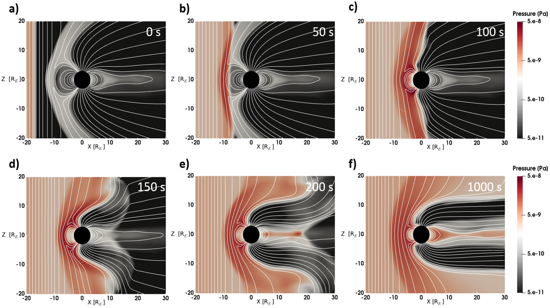
Figure 1: Gorgon pressure in the x–y plane at six instances corresponding to before, during, and after, IP Shock IV impacts the simulated magnetosphere. Selected magnetic field lines are depicted in white and the shock parameters are listed in Table 1.

The IP shock slows down upon passing through the bow shock and panel (b) shows it develops a curved front as it propagates through the dense magnetosheath (Samsonov et al., 2006; Andreeova et al., 2011). The subsequent impact on the magnetopause disrupts the pressure-balanced equilibrium which initiates the commencement phase associated with geomagnetic storms (Smith et al., 1986; Araki, 1994). The initial magnetospheric state shows pressures below 1 nPa and the enhanced solar wind pressure consequently produces magnetosheath pressures over an order of magnitude higher. The tailward propagating magnetosonic pulse, panels (d–e), subsequently produces enhanced plasma sheet pressures, thinning of the tail current sheet and induces near-Earth tail reconnection (Oliveira and Raeder, 2014). The enhanced dynamic pressure in the solar wind compresses the magnetopause boundary from its initial position near –10 R_E to its final position near –6 R_E.

3.2 Subsolar Magnetopause

The magnetopause can be characterised as possessing a finite thickness from several ion gyroradii of several hundred kilometres (Le and Russell, 1994) to over half an Earth radius (Kaufmann and Konradi, 1973). The different plasma conditions on either side results in this being an asymmetric structure. Along the sub-solar line the shocked solar wind first slows and diverts at the fluopause (Palmroth et al., 2003) which, based on the gradient of the velocity stream lines, is initially determined at $\approx$ –10.9 R_E. The southward oriented magnetic field then passes through zero at –10.75 R_E as it tends to the significantly larger positive magnetospheric fields. Further inward, the peak in the magnetopause current density is located at –10.45 R_E, which is then followed by a local depletion in the plasma density at –10.1 R_E. In this study we determine the magnetopause position using the B_z = 0 condition, which provides a consistent measure for southward IMF regardless of solar wind conditions and stand-off distance.

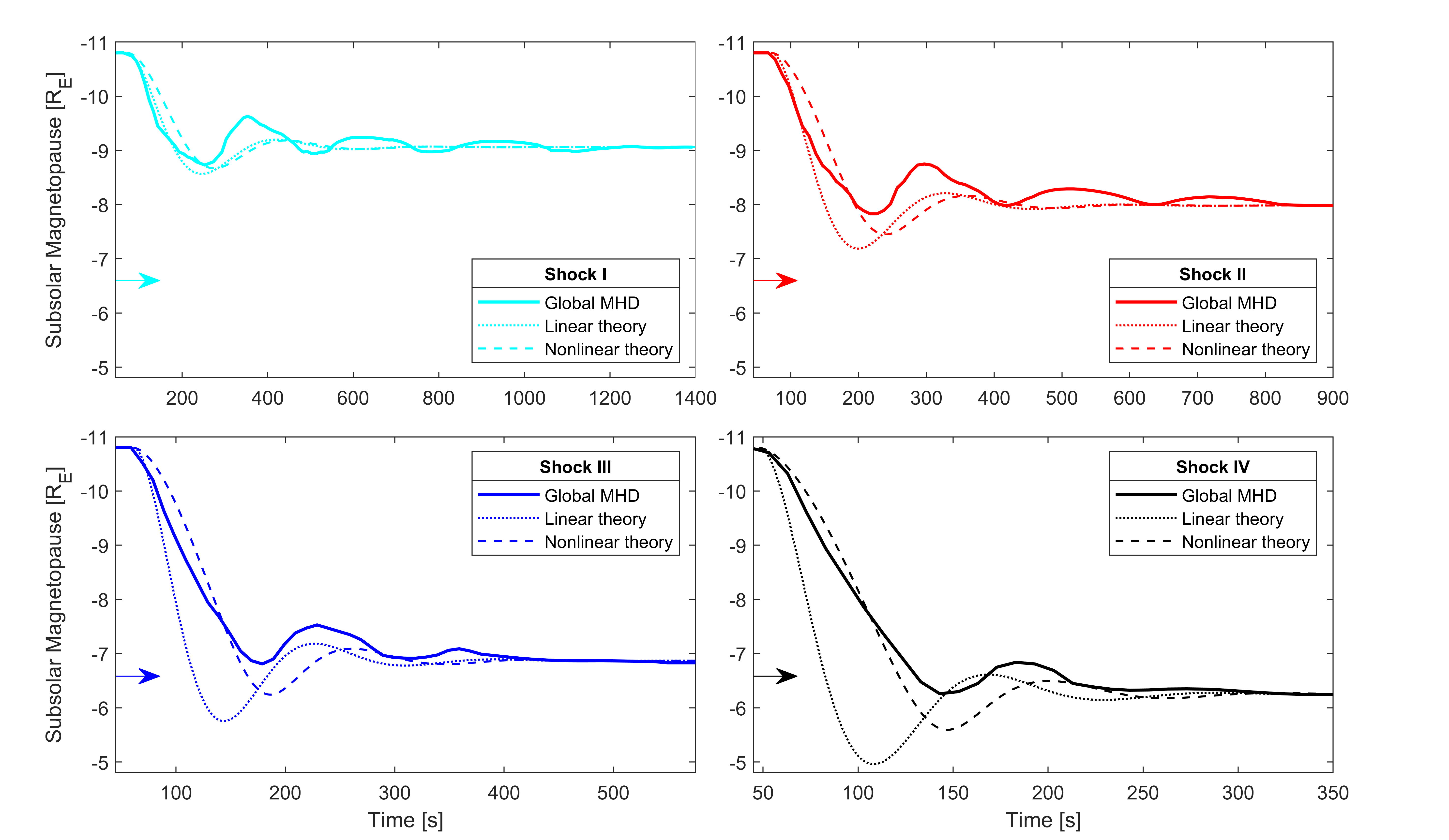
Figure 2: Simulated subsolar magnetopause stand-off distance compared to linear and nonlinear theoretical predictions for the four Shocks listed in Table 1. For reference the location of geosynchronous orbit is annotated with an arrow.

Figure 2 shows traces of the Gorgon subsolar magnetopause stand-off distances (solid lines) over time for the four shocks simulated. The motion of the magnetopause appears as three distinct phases. The first involves an acceleration as the inertia of the magnetosheath is overcome. The second appears as a rapid compressive phase which comprises the majority of the change in standoff distance. The end of this rapid compression marks the third stage of large-scale oscillatory motion with amplitudes of the order of an Earth radius before the magnetopause reaches pressure-balanced equilibrium.

Shock I has the smallest compressive phase as the final oscillations around pressure balance appear of a comparable magnitude to the total stand-off distance travelled. For increasing shock strengths, the duration of the compressive phase increases and the amplitudes and also frequencies of the oscillations appear to decrease. The underlying position about which the oscillations occur shifts Earthward as the oscillations are damped away which may be attributed to changing conditions within the sheath, see Figure 1. The oscillations also appear more strongly damped for the stronger shocks with Shock IV producing magnetopause oscillations for approximately 300 seconds compared to Shock I which produces oscillations which last four times as long. Shocks I and II also feature more oscillations than III and IV, indicating that they have a weaker damping ratio.

Also shown in Figure 2 are the subsolar magnetopause motions of the four shocks predicted by the nonlinear numerical solution of Equation 3 (dashed lines) and the linear solution given by Equation 5 (dotted lines), using c=1.2, s=1, and values for $\rho_{\infty}$, u_∞, R₀, and R_∞ taken from the simulations. As expected, the linear solution is most similar to the nonlinear numerical solution for Shock I, where the approximation r$<<$R_∞ is most valid. The difference increases with shock strength, especially in the initial phase when the second-order (dR/dt)² term in Equation 3 is not negligible. Nevertheless, the linear theory is instructive in explaining the qualitative response characteristics of a finite magnetopause response time, overshoot, and decaying oscillation. For the nonlinear theory solution, the oscillation period of the simulation produces good agreement in all cases but the initial response time and oscillation damping rate are both progressively overestimated compared to the simulation with weakening shock strength. This suggests that the second term in Equation 3 may be an oversimplification in the weak shock limit, and particularly the (dR/dt)² term within it because the linear theory that neglects (dR/dt)² actually captures the initial simulation response better than the nonlinear theory for Shocks I and II. It should also be noted that the initial response is very sensitive to the initial conditions in the magnetosheath (not shown) which may differ in the simulation from those assumed in the theory.

The linear theory is instructive in understanding the underlying physics of the magnetopause response. The nonlinear theoretical solutions of Equations 3 provide a means to extend this to larger peturbations but the solutions are still necessarily dependent on the choice of coefficients and the assumptions behind these such as the shape of the magnetopause surface and constant sheath thickness. Further effects such as magnetic reconnection, magnetosheath heating, finite solar wind mach numbers and wave speeds, and the reflection at the pulse of the inner boundary back onto the magnetopause (Li et al., 1993; Samsonov et al., 2007), are also not accounted for. The time-dependent and self-consistent numerical solutions to the MHD equations, as solved by Gorgon, instead provide the means of testing the the theory outlined in Section 2.3 for realistic nonlinear system-scale scenarios of strong fast-forward IP shock-induced magnetopause motion. Large-scale periodic magnetopause motion, consistent with those described here, have been observed following the arrival of strong fast-forward IP shocks. During the impact of the August 1972 ICME, when the sub-solar magnetopause was compressed to less than 5.2 R_E upstream, the Explorer 45 satellite experienced multiple magnetopause crossings in rapid succession (Cahill and Skillman, 1977). Similarly, during the extreme event of March 1991, the GOES-6 satellite experienced six inward-outward periodic movements of the magnetopause over a 30 minute period (Cahill and Winckler, 1992). The lack of an upstream solar wind monitor does, however, complicate further direct comparison to these events.

3.3 Frequency Analysis

The response of the magnetopause in the Gorgon simulations requires time-frequency analysis suitable for non-stationary and nonlinear processes. Figure 3 uses ensemble empirical mode decomposition (EEMD) (Wu and Huang, 2004; Torres et al., 2011) to derive the statistically significant modes associated with the magnetopause motion and a Hilbert transform spectrum shows the associated characteristic frequencies.

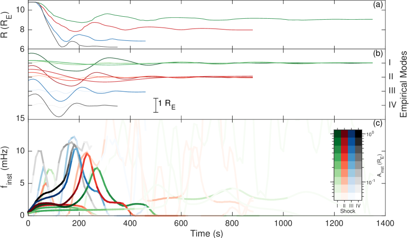
Figure 3: (a) Shows the original modes shown in Figure 2, (b) shows these decomposed into their empirical modes and (c) shows a Hilbert transform of their instantaneous frequencies.

These show the oscillations as a function of up to four statistically significant modes, the primary of which exhibit frequencies between 2–13 mHz with the frequencies of the dominant modes increasing with shock strength. The instantaneous frequencies initially increase from zero as the inertial phase begins and then plateaus somewhat during the compressive phase. They then rapidly increase during the first magnetopause rebound before relaxing back to values between 2–5 mHz. The instantaneous frequency is the time-derivative of the phase at each moment and this distinct peak is therefore interpretted as evidence of nonlinear phase steepening. Due to the strong damping, the instantaneous frequencies don’t always provide a good handle on the overall periodicity of the oscillations in each mode. Taking the auto-correlation of each mode and finding the peak, we find slightly higher overall frequencies of: 3.3, 4.1, 5.4 and 5.8 mHz for Shocks I–IV, respectively. The primary empirical modes appear strongly damped with Shocks I and II inducing approximately three total periods of diminishing amplitude whereas Shocks III and IV induce less than two such periods. The eventual periods of the oscillations are much longer than the first few oscillations for both Shocks I and II. These are being picked up by the secondary mode and the frequencies appear in the range of magnetopause surface eigenmodes being reflected between the northern and southern ionospheres (Chen and Hasegawa, 1974) as seen in high-resolution global MHD simulations (Hartinger et al., 2015) at 1.8 and 2.3 mHz respectively. With Shocks III and IV these are not apparent, possibly due to the grid resolution not sufficiently resolving field-aligned currents near the inner boundary and magnetopause reconnection at the subsolar point from the strong southward driving prohibiting a surface eigenmode forming (Plaschke and Glassmeier, 2011; Archer et al., 2019). Further modes are apparent extending up to 0.1 Hz but these likely correspond to nonlinear higher order terms.

The simulated magnetopause frequencies at the subsolar point lie where the natural frequencies of the magnetopause fall according to the theory outlined in Section 2.3. These oscillations notably occur at the lower end of the ULF range observed throughout the magnetosphere (Menk, 2011) and Freeman et al. (1995) point out that the linear theory predicts that the magnetopause acts as a low pass filter of compressional waves due to solar wind dynamic pressure variations and resonances may thus be selectively enhanced at the natural eigenfrequency and suppressed at higher frequencies. Higher frequency waves, however, could well exist further within the magnetosphere, for example via field line resonances excited by the fast magnetosonic pulse during the compression phase. The reproduction of ULF waves in global-MHD simulations can, however, be sensitive to numerical effects (Claudepierre et al., 2009) and an exploration of the magnetospheric ULF counterparts to IP shocks is therefore left for a future endeavour.

4 Conclusions

This study has examined the magnetospheric and magnetopause response to four synthetic IP shocks of varying magnitudes using Global-MHD simulations. While previous studies (Smit, 1968; Freeman et al., 1995; Børve et al., 2011) focussed on small-scale dynamic pressure changes in the upstream driver, we developed nonlinear theory suitable for large peturbations and compared these to self consistent global MHD simulations. This approach enabled the characterisation of magnetopause motion for extreme scenarios representative of fast-forward shocks striking the magnetosphere, as occur at the forefront of coronal mass ejections.

In response to the IP shocks, the simulated magnetopause notably featured large-scale oscillatory motion of the order of an Earth radius, prior to reaching pressure balance. This was readily explained when considering the driving, inertial and restoring forces associated with theory of the magnetopause as a forced damped simple harmonic oscillator. The frequencies of the oscillations occurred in the range of 2–13 mHz, predominantly occurring between 2–5 mHz. The response times and oscillation periods seen in the simulations were quantitatively consistent with the nonlinear theory, and the damping time of the oscillation was also quantitatively consistent with nonlinear theory for the stronger shocks but underestimated by theory for the weaker shocks. The initial magnetopause response was also best predicted by linear theory for the weaker shocks and by nonlinear theory for the strongest shock, which is consistent with the assumptions beyond deriving the linearised solutions.

These large-amplitude oscillations provide an explanation for periodic magnetopause motion observed following the impact of strong interplanetary shocks during the extreme space weather events of August 1972 (Cahill and Skillman, 1977) and March 1991 (Cahill and Winckler, 1992). The time-delay in the magnetopause response due to the inertia of the magnetosheath, combined with the large-scale oscillatory motion, also helps to understand why static models of the magnetopause break down during periods of strong solar wind driving (e.g. Staples et al., 2020). Furthermore, the varying structure throughout a given Earth-bound coronal mass ejection, combined with the dynamic magnetopause response, could well mean that the magnetopause rarely settles into highly compressed equilibrium states, which would also introduce a significant bias to in-situ measurements of its locations.

Rapid inward motion of the magnetopause has been observed to consistently produce enhancements and dropouts in the radiation belt phase space distributions (Reeves et al., 2003; Schiller et al., 2016) and to drive an abundance of global ultra-low-frequency wave activity (Li et al., 1997; Green and Kivelson, 2004) and enhance ionospheric and ground-induced currents (Fujita et al., 2003; Smith et al., 2019). These phenomena therefore present further observables which could be affected by and tested (e.g. Wang et al., 2010) for the large-scale magnetopause oscillations described herein.

Data Availability Statement

The simulation data used in this paper is openly available on the UK Polar Data Centre (UK PDC): https://doi.org/10.5285/3774fa5b-f2fb-42c3-9091-5b11ac9744ea

References

- Andreeova et al. [2011] K. Andreeova, T. I. Pulkkinen, L. Juusola, M. Palmroth, and O. Santolík. Propagation of a shock-related disturbance in the Earth’s magnetosphere. Journal of Geophysical Research (Space Physics), 116(A1):A01213, Jan. 2011. doi: 10.1029/2010JA015908.
- Araki [1994] T. Araki. A Physical model of the geomagnetic sudden commencement. Washington DC American Geophysical Union Geophysical Monograph Series, 81:183–200, Jan. 1994. doi: 10.1029/GM081p0183.
- Archer et al. [2019] M. O. Archer, H. Hietala, M. D. Hartinger, F. Plaschke, and V. Angelopoulos. Direct observations of a surface eigenmode of the dayside magnetopause. Nature Communications, 10:615, Feb. 2019. doi: 10.1038/s41467-018-08134-5.
- Benson [1992] D. Benson. Computational methods in Lagrangian and Eulerian hydrocodes. Computer Methods in Applied Mechanics and Engineering, 99(2-3):235–394, Sept. 1992. doi: 10.1016/0045-7825(92)90042-I.
- Berdichevsky et al. [2000] D. B. Berdichevsky, A. Szabo, R. P. Lepping, A. F. Viñas, and F. Mariani. Interplanetary fast shocks and associated drivers observed through the 23rd solar minimum by Wind over its first 2.5 years. Journ. Geophys. Res., 105(A12):27289–27314, Dec. 2000. doi: 10.1029/1999JA000367.
- Blake et al. [1992] J. B. Blake, W. A. Kolasinski, R. W. Fillius, and E. G. Mullen. Injection of electrons and protons with energies of tens of MeV into L ¡ 3 on 24 March 1991. Geophys. Res. Lett, 19(8):821–824, Apr. 1992. doi: 10.1029/92GL00624.
- Boris [1970] J. P. Boris. A physically motivated solution of the alfven problem. Tech. Rep. 2167, 1970.
- Børve et al. [2011] S. Børve, H. Sato, H. L. Pécseli, and J. K. Trulsen. Minute-scale period oscillations of the magnetosphere. Annales Geophysicae, 29(4):663–671, Apr. 2011. doi: 10.5194/angeo-29-663-2011.
- Bowe et al. [1990] G. A. Bowe, M. A. Hapgood, M. Lockwood, and D. M. Willis. Short-term variability of solar wind number density, speed and dynamic pressure as a function of the interplanetary magnetic field components: A survey over two solar cycles. Geophys. Res. Lett., 17(11):1825–1828, Oct. 1990. doi: 10.1029/GL017i011p01825.
- Burgess [1989] D. Burgess. On the effect of a tangential discontinuity on ions specularly reflected at an oblique shock. Journal of Geophys. Res., 94(A1):472–478, Jan. 1989. doi: 10.1029/JA094iA01p00472.
- Burlaga [1971] L. F. Burlaga. Hydromagnetic Waves and Discontinuities in the Solar Wind. Space Sci. Rev., 12(5):600–657, Dec. 1971. doi: 10.1007/BF00173345.
- Cahill and Skillman [1977] J. Cahill, L. J. and T. L. Skillman. The magnetopause at 5.2 RE in August 1972: Magnetopause motion. Journ. Geophys. Res., 82(10):1566, Apr. 1977. doi: 10.1029/JA082i010p01566.
- Cahill and Winckler [1992] J. Cahill, L. J. and J. R. Winckler. Periodic magnetopause oscillations observed with the GOES satellites on March 24, 1991. Journ. Geophys. Res., 97(A6):8239–8243, June 1992. doi: 10.1029/92JA00433.
- Cahill and Winckler [1999] L. J. Cahill and J. R. Winckler. Magnetopause crossings observed at 6.6RE. Journ. Geophys. Res., 104(A6):12229–12238, June 1999. doi: 10.1029/1998JA900072.
- Chapman and Ferraro [1931] S. Chapman and V. C. A. Ferraro. A new theory of magnetic storms. Terrestrial Magnetism and Atmospheric Electricity (Journal of Geophysical Research), 36(3):171, Jan. 1931. doi: 10.1029/TE036i003p00171.
- Chen and Hasegawa [1974] L. Chen and A. Hasegawa. A theory of long-period magnetic pulsations: 1. Steady state excitation of field line resonance. Journ. Geophys. Res., 79(7):1024–1032, Mar. 1974. doi: 10.1029/JA079i007p01024.
- Chittenden et al. [2004] J. P. Chittenden, S. V. Lebedev, C. A. Jennings, S. N. Bland , and A. Ciardi. X-ray generation mechanisms in three-dimensional simulations of wire array Z-pinches. Plasma Physics and Controlled Fusion, 46(12B):B457–B476, Dec. 2004. doi: 10.1088/0741-3335/46/12B/039.
- Ciardi et al. [2007] A. Ciardi, S. V. Lebedev, A. Frank, E. G. Blackman, J. P. Chittenden, C. J. Jennings, D. J. Ampleford, S. N. Bland, S. C. Bott, J. Rapley, G. N. Hall, F. A. Suzuki-Vidal, A. Marocchino, T. Lery, and C. Stehle. The evolution of magnetic tower jets in the laboratory. Physics of Plasmas, 14(5):056501–056501, May 2007. doi: 10.1063/1.2436479.
- Claudepierre et al. [2009] S. G. Claudepierre, M. Wiltberger, S. R. Elkington, W. Lotko, and M. K. Hudson. Magnetospheric cavity modes driven by solar wind dynamic pressure fluctuations. Geophys. Res. Lett., 36(13):L13101, July 2009. doi: 10.1029/2009GL039045.
- Desai et al. [2020] R. T. Desai, H. Zhang, E. E. Davies, J. E. Stawarz, J. Mico-Gomez, and P. Iváñez-Ballesteros. Three-Dimensional Simulations of Solar Wind Preconditioning and the 23 July 2012 Interplanetary Coronal Mass Ejection. Solar Physics, 295(9):130, Sept. 2020. doi: 10.1007/s11207-020-01700-5.
- Dungey [1961] J. W. Dungey. Interplanetary Magnetic Field and the Auroral Zones. Phys. Rev. Lett., 6(2):47–48, Jan. 1961. doi: 10.1103/PhysRevLett.6.47.
- Echer et al. [2003] E. Echer, W. D. Gonzalez, L. E. A. Vieira, A. Dal Lago, F. L. Guarnieri, A. Prestes, A. L. C. Gonzalez, and N. J. Schuch. Interplanetary shock parameters during solar activity maximum (2000) and minimum (1995-1996). Brazilian Journal of Physics, 33(1):115–122, Mar. 2003. doi: 10.1590/S0103-97332003000100010.
- Eggington et al. [2018] J. W. B. Eggington, L. Mejnertsen, R. T. Desai, J. P. Eastwood, and J. P. Chittenden. Forging links in Earth’s plasma environment. Astronomy and Geophysics, 59(6):6.26–6.28, Dec. 2018. doi: 10.1093/astrogeo/aty275.
- Eggington et al. [2020] J. W. B. Eggington, J. P. Eastwood, L. Mejnertsen, R. T. Desai, and J. P. Chittenden. Dipole Tilt Effect on Magnetopause Reconnection and the Steady-State Magnetosphere-Ionosphere System: Global MHD Simulations. Journal of Geophysical Research (Space Physics), 125(7):e27510, July 2020. doi: 10.1029/2019JA027510.
- Freeman et al. [1995] M. P. Freeman, N. C. Freeman, and C. J. Farrugia. A linear perturbation analysis of magnetopause motion in the Newton-Busemann limit. Annales Geophysicae, 13(9):907–918, Sept. 1995. doi: 10.1007/s00585-995-0907-0.
- Freeman et al. [1998] M. P. Freeman, N. C. Freeman, and C. J. Farrugia. Magnetopause Motions in a Newton-Busemann Approach. Moen J., Egeland A., Lockwood M. (eds) Polar Cap Boundary Phenomena. NATO ASI Series (Series C: Mathematical and Physical Sciences), 13(9):907–918, Sept. 1998. doi: https://doi.org/10.1007/978-94-011-5214-3-2.
- Fujita et al. [2003] S. Fujita, T. Tanaka, T. Kikuchi, K. Fujimoto, K. Hosokawa, and M. Itonaga. A numerical simulation of the geomagnetic sudden commencement: 1. Generation of the field-aligned current associated with the preliminary impulse. Journal of Geophysical Research (Space Physics), 108(A12):1416, Dec. 2003. doi: 10.1029/2002JA009407.
- Gopalswamy et al. [2005] N. Gopalswamy, S. Yashiro, Y. Liu, G. Michalek, A. Vourlidas, M. L. Kaiser, and R. A. Howard. Coronal mass ejections and other extreme characteristics of the 2003 October-November solar eruptions. Journal of Geophysical Research (Space Physics), 110(A9):A09S15, Sept. 2005. doi: 10.1029/2004JA010958.
- Green and Kivelson [2004] J. C. Green and M. G. Kivelson. Relativistic electrons in the outer radiation belt: Differentiating between acceleration mechanisms. Journal of Geophysical Research (Space Physics), 109(A3):A03213, Mar. 2004. doi: 10.1029/2003JA010153.
- Hartinger et al. [2015] M. D. Hartinger, F. Plaschke, M. O. Archer, D. T. Welling, M. B. Moldwin, and A. Ridley. The global structure and time evolution of dayside magnetopause surface eigenmodes. Geophys. Res. Lett., 42(8):2594–2602, Apr. 2015. doi: 10.1002/2015GL063623.
- Hietala et al. [2009] H. Hietala, T. V. Laitinen, K. Andréeová, R. Vainio, A. Vaivads, M. Palmroth, T. I. Pulkkinen, H. E. J. Koskinen, E. A. Lucek, and H. Rème. Supermagnetosonic Jets behind a Collisionless Quasiparallel Shock. Phys. Rev. Lett., 103(24):245001, Dec. 2009. doi: 10.1103/PhysRevLett.103.245001.
- Horne and Pitchford [2015] R. B. Horne and D. Pitchford. Space Weather Concerns for All-Electric Propulsion Satellites. Space Weather, 13(8):430–433, Aug. 2015. doi: 10.1002/2015SW001198.
- Hudson et al. [1997] M. K. Hudson, S. R. Elkington, J. G. Lyon, V. A. Marchenko, I. Roth, M. Temerin, J. B. Blake, M. S. Gussenhoven, and J. R. Wygant. Simulations of radiation belt formation during storm sudden commencements. Journ. Geophys. Res., 102(A7):14087–14102, July 1997. doi: 10.1029/97JA03995.
- Kaufmann and Konradi [1973] R. L. Kaufmann and A. Konradi. Speed and thickness of the magnetopause. Journ. Geophys. Res., 78(28):6549, Jan. 1973. doi: 10.1029/JA078i028p06549.
- Kennel et al. [1985] C. F. Kennel, J. P. Edmiston, and T. Hada. A quarter century of collisionless shock research. Washington DC American Geophysical Union Geophysical Monograph Series, 34:1–36, Jan. 1985. doi: 10.1029/GM034p0001.
- Kivelson et al. [1984] M. G. Kivelson, J. Etcheto, and J. G. Trotignon. Global compressibional oscillations of the terrestrial magnetosphere: The evidence and a model. Journal of Geophys. Res., 89(A11):9851–9856, Nov. 1984. doi: 10.1029/JA089iA11p09851.
- Le and Russell [1994] G. Le and C. T. Russell. The thickness and structure of high beta magnetopause current layer. Geophys. Res. Lett., 21(23):2451–2454, Nov. 1994. doi: 10.1029/94GL02292.
- Li et al. [1993] X. Li, I. Roth, M. Temerin, J. R. Wygant, M. K. Hudson, and J. B. Blake. Simulation of the prompt energization and transport of radiation belt particles during the march 24, 1991 ssc. Geophysical Research Letters, 20(22):2423–2426, 1993. doi: https://doi.org/10.1029/93GL02701. URL https://agupubs.onlinelibrary.wiley.com/doi/abs/10.1029/93GL02701.
- Li et al. [1997] X. Li, D. N. Baker, M. Temerin, T. E. Cayton, E. G. D. Reeves, R. A. Christensen, J. B. Blake, M. D. Looper, R. Nakamura, and S. G. Kanekal. Multisatellite observations of the outer zone electron variation during the November 3-4, 1993, magnetic storm. Journ. Geophys. Res., 102(A7):14123–14140, July 1997. doi: 10.1029/97JA01101.
- Lin et al. [2010] R. L. Lin, X. X. Zhang, S. Q. Liu, Y. L. Wang, and J. C. Gong. A three-dimensional asymmetric magnetopause model. Journal of Geophysical Research (Space Physics), 115(A4):A04207, Apr. 2010. doi: 10.1029/2009JA014235.
- Mead and Beard [1964] G. D. Mead and D. B. Beard. Shape of the Geomagnetic Field Solar Wind Boundary. Journ. Geophys. Res., 69(7):1169–1179, Apr. 1964. doi: 10.1029/JZ069i007p01169.
- Mejnertsen et al. [2016] L. Mejnertsen, J. P. Eastwood, J. P. Chittenden, and A. Masters. Global mhd simulations of neptune’s magnetosphere. Journal of Geophysical Research: Space Physics, 121(8):7497–7513, 2016. doi: 10.1002/2015JA022272. URL https://agupubs.onlinelibrary.wiley.com/doi/abs/10.1002/2015JA022272.
- Mejnertsen et al. [2018] L. Mejnertsen, J. P. Eastwood, H. Hietala, S. J. Schwartz, and J. P. Chittenden. Global MHD Simulations of the Earth’s Bow Shock Shape and Motion Under Variable Solar Wind Conditions. Journal of Geophysical Research (Space Physics), 123(1):259–271, Jan. 2018. doi: 10.1002/2017JA024690.
- Menk [2011] F. W. Menk. Magnetospheric ULF Waves: A Review, pages 223–256. Springer Netherlands, Dordrecht, 2011. ISBN 978-94-007-0501-2. doi: 10.1007/978-94-007-0501-2-13. URL https://doi.org/10.1007/978-94-007-0501-2-13.
- Meredith et al. [2017] N. P. Meredith, R. B. Horne, I. Sandberg, C. Papadimitriou, and H. D. R. Evans. Extreme relativistic electron fluxes in the Earth’s outer radiation belt: Analysis of INTEGRAL IREM data. Space Weather, 15(7):917–933, July 2017. doi: 10.1002/2017SW001651.
- Merka et al. [2003] J. Merka, A. Szabo, J. Šafránková, and Z. Němeček. Earth’s bow shock and magnetopause in the case of a field-aligned upstream flow: Observation and model comparison. Journal of Geophysical Research (Space Physics), 108(A7):1269, July 2003. doi: 10.1029/2002JA009697.
- Němeček et al. [2016] Z. Němeček, J. Šafránková, R. E. Lopez, Š. Dušík, L. Nouzák, L. Přech, J. Šimůnek, and J. H. Shue. Solar cycle variations of magnetopause locations. Advances in Space Research, 58(2):240–248, July 2016. doi: 10.1016/j.asr.2015.10.012.
- Oliveira and Raeder [2014] D. M. Oliveira and J. Raeder. Impact angle control of interplanetary shock geoeffectiveness. Journal of Geophysical Research (Space Physics), 119(10):8188–8201, Oct. 2014. doi: 10.1002/2014JA020275.
- Omidi et al. [2010] N. Omidi, J. P. Eastwood, and D. G. Sibeck. Foreshock bubbles and their global magnetospheric impacts. Journal of Geophysical Research (Space Physics), 115(A6):A06204, June 2010. doi: 10.1029/2009JA014828.
- Palmroth et al. [2003] M. Palmroth, T. I. Pulkkinen, P. Janhunen, and C. C. Wu. Stormtime energy transfer in global MHD simulation. Journal of Geophysical Research (Space Physics), 108(A1):1048, Jan. 2003. doi: 10.1029/2002JA009446.
- Plaschke and Glassmeier [2011] F. Plaschke and K.-H. Glassmeier. Properties of standing kruskal-schwarzschild-modes at the magnetopause. Annales Geophysicae, 29(10):1793–1807, 2011. doi: 10.5194/angeo-29-1793-2011. URL https://angeo.copernicus.org/articles/29/1793/2011/.
- Priest [1982] E. Priest. Solar Magnetohydrodynamics. Springer, 1982. doi: 10.1007/978-94-009-7958-1.
- Raeder [2003] J. Raeder. Global Magnetohydrodynamics - A Tutorial, volume 615, pages 212–246. Büchner, J. and Dum, C. and Scholer, M., 2003.
- Reeves et al. [2003] G. D. Reeves, K. L. McAdams, R. H. W. Friedel, and T. P. O’Brien. Acceleration and loss of relativistic electrons during geomagnetic storms. Geophys. Res. Lett., 30(10):1529, May 2003. doi: 10.1029/2002GL016513.
- Ridley et al. [2004] A. Ridley, T. Gombosi, and D. Dezeeuw. Ionospheric control of the magnetosphere: conductance. Annales Geophysicae, 22(2):567–584, Feb. 2004. doi: 10.5194/angeo-22-567-2004.
- Riley [2012] P. Riley. On the probability of occurrence of extreme space weather events. Space Weather, 10(2):02012, Feb. 2012. doi: 10.1029/2011SW000734.
- Russell et al. [2013] C. T. Russell, R. A. Mewaldt, J. G. Luhmann, G. M. Mason, T. T. von Rosenvinge, C. M. S. Cohen, R. A. Leske, R. Gomez-Herrero, A. Klassen, A. B. Galvin, and K. D. C. Simunac. The Very Unusual Interplanetary Coronal Mass Ejection of 2012 July 23: A Blast Wave Mediated by Solar Energetic Particles. Astrophys. Journ., 770(1):38, June 2013. doi: 10.1088/0004-637X/770/1/38.
- Samsonov et al. [2006] A. A. Samsonov, Z. Němeček, and J. Šafránková. Numerical MHD modeling of propagation of interplanetary shock through the magnetosheath. Journal of Geophysical Research (Space Physics), 111(A8):A08210, Aug. 2006. doi: 10.1029/2005JA011537.
- Samsonov et al. [2007] A. A. Samsonov, D. G. Sibeck, and J. Imber. MHD simulation for the interaction of an interplanetary shock with the Earth’s magnetosphere. Journal of Geophysical Research (Space Physics), 112(A12):A12220, Dec. 2007. doi: 10.1029/2007JA012627.
- Samsonov et al. [2020] A. A. Samsonov, Y. V. Bogdanova, G. Branduardi-Raymont, D. G. Sibeck, and G. Toth. Is the Relation Between the Solar Wind Dynamic Pressure and the Magnetopause Standoff Distance so Straightforward? Geophys. Res. Lett, 47(8):e86474, Apr. 2020. doi: 10.1029/2019GL086474.
- Schiller et al. [2016] Q. Schiller, S. G. Kanekal, L. K. Jian, X. Li, A. Jones, D. N. Baker, A. Jaynes, and H. E. Spence. Prompt injections of highly relativistic electrons induced by interplanetary shocks: A statistical study of Van Allen Probes observations. Geophys. Res. Lett., 43(24):12,317–12,324, Dec. 2016. doi: 10.1002/2016GL071628.
- Shprits et al. [2006] Y. Y. Shprits, R. M. Thorne, R. Friedel, G. D. Reeves, J. Fennell, D. N. Baker, and S. G. Kanekal. Outward radial diffusion driven by losses at magnetopause. Journal of Geophysical Research (Space Physics), 111(A11):A11214, Nov. 2006. doi: 10.1029/2006JA011657.
- Shue et al. [1998] J. H. Shue, P. Song, C. T. Russell, J. T. Steinberg, J. K. Chao, G. Zastenker, O. L. Vaisberg, S. Kokubun, H. J. Singer, T. R. Detman, and H. Kawano. Magnetopause location under extreme solar wind conditions. Journal of Geophys. Res., 103(A8):17691–17700, Aug. 1998. doi: 10.1029/98JA01103.
- Sibeck et al. [2002] D. G. Sibeck, T. D. Phan, R. Lin, R. P. Lepping, and A. Szabo. Wind observations of foreshock cavities: A case study. Journal of Geophysical Research (Space Physics), 107(A10):1271, Oct. 2002. doi: 10.1029/2001JA007539.
- Smit [1968] G. R. Smit. Oscillatory motion of the nose region of the magnetopause. Journal of Geophys. Res., 73(15):4990–4993, Aug. 1968. doi: 10.1029/JA073i015p04990.
- Smith et al. [2019] A. W. Smith, M. P. Freeman, I. J. Rae, and C. Forsyth. The Influence of Sudden Commencements on the Rate of Change of the Surface Horizontal Magnetic Field in the United Kingdom. Space Weather, 17(11):1605–1617, Nov. 2019. doi: 10.1029/2019SW002281.
- Smith and Wolfe [1976] E. J. Smith and J. H. Wolfe. Observations of interaction regions and corotating shocks between one and five AU: Pioneers 10 and 11. Geophys. Res. Lett., 3(3):137–140, Mar. 1976. doi: 10.1029/GL003i003p00137.
- Smith et al. [1986] E. J. Smith, J. A. Slavin, R. D. Zwickl, and S. J. Bame. Shocks and Storm Sudden Commencements, volume 126, page 345. Kamide, Y. and Slavin, James Arthur, 1986. doi: 10.1007/978-90-277-2303-1-25.
- Southwood [1974] D. J. Southwood. Some features of field line resonances in the magnetosphere. Plan. Space. Sci., 22(3):483–491, Mar. 1974. doi: 10.1016/0032-0633(74)90078-6.
- Staples et al. [2020] F. A. Staples, I. J. Rae, C. Forsyth, A. R. A. Smith, K. R. Murphy, K. M. Raymer, F. Plaschke, N. A. Case, C. J. Rodger, J. A. Wild, S. E. Milan, and S. M. Imber. Do Statistical Models Capture the Dynamics of the Magnetopause During Sudden Magnetospheric Compressions? Journal of Geophysical Research (Space Physics), 125(4):e27289, Apr. 2020. doi: 10.1029/2019JA027289.
- Tanaka [1994] T. Tanaka. Finite Volume TVD Scheme on an Unstructured Grid System for Three-Dimensional MHD Simulation of Inhomogeneous Systems Including Strong Background Potential Fields. Journal of Computational Physics, 111(2):381–389, Apr. 1994. doi: 10.1006/jcph.1994.1071.
- Torres et al. [2011] M. E. Torres, M. A. Colominas, G. Schlotthauer, and P. Flandrin. A complete ensemble empirical mode decomposition with adaptive noise. In 2011 IEEE International Conference on Acoustics, Speech and Signal Processing (ICASSP), pages 4144–4147, 2011. doi: 10.1109/ICASSP.2011.5947265.
- Tsurutani and Lakhina [2014] B. T. Tsurutani and G. S. Lakhina. An extreme coronal mass ejection and consequences for the magnetosphere and Earth. Geophys. Res. Lett., 41(2):287–292, Jan. 2014. doi: 10.1002/2013GL058825.
- Wang et al. [2010] C. Wang, Q. Zong, and Y. Wang. Propagation of interplanetary shock excited ultra low frequency (ULF) waves in magnetosphere-ionosphere-atmosphere—Multi-spacecraft “Cluster” and ground-based magnetometer observations. Science in China E: Technological Sciences, 53(9):2528–2534, Sept. 2010. doi: 10.1007/s11431-010-4064-7.
- Wu and Huang [2004] Z. Wu and N. E. Huang. A study of the characteristics of white noise using the empirical mode decomposition method. Proceedings of the Royal Society of London Series A, 460(2046):1597–1611, June 2004. doi: 10.1098/rspa.2003.1221.
- Yashiro et al. [2004] S. Yashiro, N. Gopalswamy, G. Michalek, O. C. St. Cyr, S. P. Plunkett, N. B. Rich, and R. A. Howard. A catalog of white light coronal mass ejections observed by the SOHO spacecraft. Journal of Geophysical Research (Space Physics), 109(A7):A07105, July 2004. doi: 10.1029/2003JA010282.
- Yee [1966] K. S. Yee. Numerical solution of initial boundary value problems involving maxwell’s equations in isotropic media. IEEE Trans. Antennas and Propagation, pages 302–307, 1966.