Multiplexed telecom-band quantum networking with atom arrays in optical cavities

Abstract

The realization of a quantum network node of matter-based qubits compatible with telecom-band operation and large-scale quantum information processing is an outstanding challenge that has limited the potential of elementary quantum networks. We propose a platform for interfacing quantum processors comprising neutral atom arrays with telecom-band photons in a multiplexed network architecture. The use of a large atom array instead of a single atom mitigates the deleterious effects of two-way communication and improves the entanglement rate between two nodes by nearly two orders of magnitude. Further, this system simultaneously provides the ability to perform high-fidelity deterministic gates and readout within each node, opening the door to quantum repeater and purification protocols to enhance the length and fidelity of the network, respectively. Using intermediate nodes as quantum repeaters, we demonstrate the feasibility of entanglement distribution over $\approx 1500\,\text{km}$ based on realistic assumptions, providing a blueprint for a transcontinental network. Finally, we demonstrate that our platform can distribute $\gtrsim 25$ Bell pairs over metropolitan distances, which could serve as the backbone of a distributed fault-tolerant quantum computer.

I Introduction

The development of a robust quantum network Cirac1997 ; Wehner2018 ; Kimble2008 will usher in an era of cryptographically-secured communication Pirandola2019 , distributed and blind quantum computing Jiang2007 , and sensor and clock networks operating with precision at the fundamental limit Komar2014 . Almost all of these applications require network nodes that are capable of storing, processing, and distributing quantum information and entanglement over large distances Kimble2008 . Nodes based on neutral atoms have the potential to combine highly desirable features including minute-scale coherence and memory times Young2020 , scalability to hundreds of qubits per node Ebadi2020 , multi-qubit processing capabilities Saffman2010 ; Levine2019 ; Graham2019 , and efficient light-matter interfaces at telecom wavelengths Uphoff2016 ; Covey2019b ; Menon2020 based on optical cavities Kimble2008 ; Reiserer2015 .

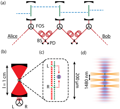
FIG. 1: Overview of the network architecture. (a) Nodes based on arrays of atoms (green circles) in optical cavities generate a Bell pair over each link (blue dashes) to distribute entanglement between end-users Alice and Bob. We employ “heralded” entanglement generation based on photon interference on a 50:50 beamsplitter (BS). Fiber-optic switches (FOS) connect adjacent nodes at will by routing the photons from each cavity. (b) The near-concentric optical cavities have a mirror spacing of $\approx 1\,\text{cm}$ while the atom array spans a length of only $\approx 200$ $\mu$m. (c) The time signature of the photons on the detectors (PD) informs which atoms at each node are in a Bell state (green check marks). Subsequent, deterministic gates can be achieved by moving these atoms (dashed red arrows) and performing Rydberg entangling operations (purple circle). (d) A standing wave in the cavity traps atoms in a one-dimensional array (blue) to overlap with the highest field strength of the telecom mode (red). Atoms are positioned with auxiliary optical tweezers (yellow) that also move the atoms.

Despite recent work establishing neutral atom-based nodes Ritter2012 ; Hofmann2012 ; Samutpraphoot2020 ; Langenfeld2021 ; Daiss2021 ; Dordevic2021 , a major bottleneck for the development of such a network is the exponential attenuation and long transit time associated with sending single photons – the quantum bus that distributes entanglement – throughout the network Reiserer2015 . Since the success probability per entanglement generation attempt is low and success must be “heralded” via two-way communication Duan2001 ; Pfaff2013 , there is intense interest in developing architectures that can “multiplex” many signals in parallel on each attempt Graham2013 ; Sinclair2014 ; Kaneda2015 ; Zhong2017 ; Wengerowsky2018 . Multiplexing is necessary to construct networks much larger than the attenuation length in optical fiber ($\approx$20 km in the telecom band Corning2020 ), but it not sufficient. Intermediate “repeater” nodes are required to swap the entanglement and teleport quantum information Duan2001 ; Pirandola2019 . Additionally, entanglement “purification” protocols Dur2003 ; Bennett1996a ; Kalb2017 are often needed to improve the fidelity of the distributed quantum states.

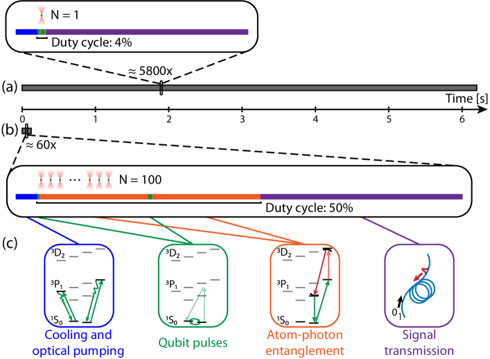
FIG. 2: Multiplexed remote entanglement generation over $L=100\,\text{km}$ with atom arrays. (a) With only a single atom at each node, the low success probability necessitates an average of $\approx 5800$ entanglement attempts. The solid gray bar shows this process with time moving to the right. The zoom shows a single attempt, in which the cooling and initialization of the atom (blue) and signal transmission over the link (purple) dominate the duration of each attempt. The duty cycle of entanglement-producing operations – qubit rotations (green) and atom-photon entanglement (orange) [see Fig. 3 for details] – is only $\approx 4$%. (b) With an array of $N=100$ atoms at each node, the success probability necessitates an average of only $\approx 60$ multiplexed attempts; hence the overall time it takes to create entanglement (gray bar) is much shorter. Each attempt takes longer and has a much greater duty cycle of $\approx 50$% for entanglement-producing operations. (c) A cartoon of the operations required for each attempt. The two qubit rotations and atom-photon entanglement operations follow the standard protocol for time-bin entanglement generation Barrett2005 ; Bernien2013 .

Here, we propose a quantum network and repeater node architecture that is capable of high-rate, multiplexed entanglement generation, deterministic inter-node quantum gates and Bell-state measurements for purification and distribution of many-body states, while at the same time operating at telecom wavelengths where low-loss optical fibers permit long-distance entanglement distribution. Our architecture is based on arrays Endres2016 ; Barredo2016 of individual neutral ytterbium (Yb) atoms, an alkaline earth-like species Cooper2018 ; Norcia2018b ; Saskin2019 , in large ($\approx 1\,\text{cm}$), near-concentric optical cavities Casabone2013 ; Nguyen2018 ; Davis2019 ; Zeiher2020 (see Fig. 1). We consider a time-bin entanglement generation protocol Bernien2013 that combines a strong, $1.48$ $\mu$m-wavelength transition Covey2019b ; Covey2019c and long-lived nuclear spin-1/2 qubit states of ${}^{171}\text{Yb}$ with temporal multiplexing along the array of atoms.

Based on recent progress with alkaline-earth atomic arrays Cooper2018 ; Norcia2018b ; Saskin2019 ; Covey2019 ; Norcia2019 ; Madjarov2019 ; Madjarov2020 ; Wilson2019 and realistic assumptions regarding the operation of these nodes, we show that our multiplexing protocol can generate Bell pairs over $>1000$ kilometers within the coherence time of the qubits, and is compatible with entanglement purification protocols Dur2003 ; Bennett1996a ; Kalb2017 as well as the distribution of many-body states Komar2014 ; Polzik2016 ; Bernien2017 ; Choi2021 . Our work lays the foundation for a versatile metropolitan or transcontinental network through a novel architecture that combines the use of Rydberg atom arrays Saffman2010 ; Browaeys2020 , cavity QED with strong atom-photon coupling McKeever2003 ; Birnbaum2005 ; Tiecke2014 ; Reiserer2015 , and atom-array optical clocks Madjarov2019 ; Norcia2019 ; Young2020 in one platform for the first time.

II Multiplexed remote entanglement generation

To motivate the proposed architecture, we begin with an overview of our multiplexed time-bin networking protocol. Specifically, we consider the example of a network link of length $L=100\,\text{km}$. The associated two-way signal transmission time per attempt is $\tau=2L/c$, where $c=c_{0}/n$ is the speed of light in optical fiber ($n=1.4$) that includes both the quantum signal and classical heralding signal; $\tau\approx 1\,\text{ms}$ for this distance. Per the methods described below, we estimate that $\approx 5800$ entanglement attempts will be required if there is only a single qubit (atom) at each node, resulting in a $\approx 0.16\,\text{Hz}$ entanglement generation rate. Figure 2(a) shows the full process of successful entanglement generation with a zoomed view of each attempt. The attempt time is dominated by signal transmission (see Appendix D for full timing details) such that the duty cycle of entanglement-producing operations is only $\approx 4\%$.

If instead we have $N=100$ qubits at each node and multiplex their signals as described below, we can drastically decrease the number of required attempts to only $\approx 60$ resulting in a $\approx 50$-fold increase in the entanglement rate to $8\,\text{Hz}$ at $L=100\,\text{km}$. Figure 2(b) shows the full process of successful entanglement generation for $N=100$ atoms with a zoomed view of each multiplexed attempt. In this case the duty cycle for entanglement-producing operations is $\approx 50\%$. Although the time required per attempt is longer when multiplexing across a large number of atoms, the favorable scaling in success probability per attempt over long network links leads to substantially improved entanglement generation rates compared to the case of a single atom.

III Description of the network architecture

Before summarizing these results in more detail in section IV and V, we provide an overview of the atom array platform and the atom-photon entanglement scheme. Further details on these topics can be found in Appendices B and C, respectively.

III.1 Atom arrays in near-concentric optical cavities

There has been intense interest in coupling neutral atoms to optical cavities with small mode volumes such as nanophotonic Samutpraphoot2020 ; Dordevic2021 ; Menon2020 and fiber-gap Fabry-Pérot Hunger2010 ; Haas2014 ; Brekenfeld2020 systems to enhance the atom-photon coupling. However, these systems are not readily compatible with large atom arrays (and single-atom control therein) due to their limited optical accessibility. Additionally, the proximity of dielectric surfaces to the atoms makes the prospect for robust, high-fidelity Rydberg-mediated gates uncertain as stray electric fields limit the coherence of Rydberg transitions Sedlacek2016 ; Thiele2015 .

Meanwhile, near-concentric cavities with large mirror spacings ($\ell\gtrsim 1\,\text{cm}$) have recently been used with great success in myriad cavity QED research directions Casabone2013 ; Nguyen2018 ; Davis2019 ; Zeiher2020 , and offer enough optical access to enable single-atom control in cavity-coupled atom arrays. Crucially, the mirror spacing is similar to the size of glass cells used in many recent high-fidelity Rydberg entanglement studies Levine2019 ; Graham2019 ; Madjarov2020 ; Wilson2019 . Further, near-concentric cavities are widely used in trapped ion systems Casabone2013 that are also sensitive to transient electric fields from dielectric surfaces Teller2021 . Therefore it is reasonable to expect that these cavities are compatible with deterministic Rydberg-mediated gates and Bell state measurements needed in a quantum repeater and purification architecture.

We focus on a near-concentric system with $\ell=0.975\,\text{cm}$ and radius of curvature $R=5\,\text{mm}$ for which the cavity stability parameter $\mathcal{G}=1-\ell/R=-0.95$ Nguyen2018 ; Kawasaki2019 . We choose a single-sided cavity, where the reflectivity of one mirror is much greater than the other to allow photon passage, with a finesse of $50,000$. We couple this cavity to the ${{}^{3}\text{P}_{1}\leftrightarrow{}^{3}\text{D}_{2}}$ transition with wavelength $\lambda_{\text{net}}=1480\,\text{nm}$ and decay rate $\Gamma=2\pi\times 318\,\text{kHz}$. Based on these parameters, the coupling strength to the cavity is $g_{34}\approx 2\pi\times 1.53\,\text{MHz}$ and the single-atom cooperativity is $C\approx 16$ (for a detailed derivation see Appendix B).

We trap the atoms in a standing wave at $\lambda_{\text{trap}}=\lambda_{\text{net}}/2=740\,\text{nm}$ to ensure maximal coupling with the telecom field (at $\lambda_{\text{net}}$) in the cavity [see Fig. 1(d)]. The standing wave at $\lambda_{\text{trap}}$ is fortuitously close to the ‘magic’ wavelength for the optical clock transition (${}^{1}\text{S}_{0}\leftrightarrow{}^{3}\text{P}_{0}$) where the two states have equal polarizability Ye2008 : $\lambda_{\text{m}}=760\,\text{nm}$. The expected $1/e^{2}$ waist radius for this standing wave is $w_{\text{trap}}\approx 14$ $\mu$m; the trap depth (and frequency) are free parameters. Optical tweezers are employed to create an atom array from the magneto-optical trap (MOT) before the standing wave is turned on, and the tweezers are positioned to overlap the desired anti-nodes of the standing wave [see Fig. 1(d)]. The standing wave provides strong axial confinement with $\lambda_{\text{trap}}/2$ spacing between the anti-nodes and guaranteed maximal overlap with the anti-nodes of telecom cavity mode at $\lambda_{\text{net}}$, and the tweezers provide strong transverse confinement.

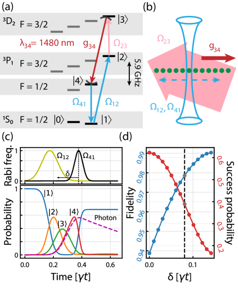
FIG. 3: Multiplexed remote entanglement via a four-pulse excitation scheme. (a) A minimal diagram of the ${}^{171}\text{Yb}$ level structure showing two hyperfine Zeeman states in the ${}^{3}\text{P}_{1}$ manifold as intermediaries. (b) Local application of $\Omega_{12}$ and $\Omega_{41}$ on an atom-by-atom level is the primary mechanism for our time-based multiplexing scheme. (c) Analysis of the pulses and internal dynamics during the process as well as the temporal shape of the extracted photon that is entangled with the nuclear qubit in the ground state. The black arrow highlights that the relative timing of the two pulses $\Omega_{12}$ and $\Omega_{41}$ is a free parameter. The maximum Rabi frequencies of these pulses are $\{\Omega_{12}^{\text{max}},\Omega_{34}^{\text{max}}\}=\{13.2\gamma,23.0\gamma\}$ and $\gamma=2\pi\times 180\,\text{kHz}$ is the decay rate of ${}^{3}\text{P}_{1}$. (d) The resulting atom-photon entanglement fidelity and success probability vs the relative timing $\delta$ of $\Omega_{12}$ and $\Omega_{41}$ in units of $\gamma$. [(c) corresponds to $\delta=0$.] We choose $\delta$ as shown in the black dashed line for the remainder of this work.

III.2 Atom-photon entanglement via four-wave mixing

We entangle the nuclear spin-$1/2$ qubit in the ground state of ${}^{171}\text{Yb}$ with a $1480\,\text{nm}$-photon on the ${{}^{3}\text{P}_{1}\leftrightarrow{}^{3}\text{D}_{2}}$ transition via a four-pulse scheme that uses two Zeeman states within the ${}^{3}\text{P}_{1}$ manifold as intermediaries [see Fig. 3(a)]. The target state of our protocol is the atom-photon Bell state ${|\psi\rangle}_{\text{atom-photon}}=({|0\rangle}_{a}{|\text{early}\rangle}_{p}+{|1\rangle}_{a}{|\text{late}\rangle}_{p})/\sqrt{2}$, in which the atomic qubit states {${|0\rangle}_{a},{|1\rangle}_{a}$} are entangled with the photon occupation in an early and late emission time bin {${|\text{early}\rangle}_{p},{|\text{late}\rangle}_{p}$} Barrett2005 ; Bernien2013 . Such time-bin encoded states are ideally suited for long-distance entanglement distribution via optical fibers as they are robust against birefringence in fibers that would adversely affect other encodings such as polarization encoded states. To create ${|\psi\rangle}_{\text{atom-photon}}$ we start by preparing a superposition of the atomic qubit states $({|0\rangle}_{a}+{|1\rangle}_{a})/\sqrt{2}$. Then a coherent atomic pulse sequence results in the emission of a photon into the cavity mode only if the atom is in ${|1\rangle}$. The proposed four-level system that allows such a state selective emission is shown in Fig. 3(a), and was inspired by similar sequences that have recently been considered for alkali species Menon2020 . After the emission in the early time bin, a $\pi-$pulse on the qubit states flips ${|0\rangle}_{a}$ and ${|1\rangle}_{a}$, and second optical pulse sequence causes emission in the late time bin. This completes the protocol and leaves the system in the target state ${|\psi\rangle}_{\text{atom-photon}}$.

We leverage the $F=3/2$ and $F=1/2$ hyperfine structure of the ${}^{3}\text{P}_{1}$ manifold to provide the well-separated intermediate states ${|2\rangle}$ and ${|4\rangle}$, and we assume a magnetic field of $B\gtrsim 100$ G although this is not strictly necessary. We apply Gaussian pulses $\Omega_{12}$ and $\Omega_{41}$ on a per-atom basis within the array [Fig. 3(b)] as the primary mechanism for our time-based multiplexing scheme. $\Omega_{23}$ and $g_{34}$ couple to all atoms globally, but are distantly off-resonant with negligible differential effect on the qubit ${|0\rangle}-{|1\rangle}$ when $\Omega_{12}$ and $\Omega_{41}$ are not applied to the atom. Hence, we raster the tightly-focused $\Omega_{12}$ and $\Omega_{41}$ beams across the atoms such that the position of the atom in the array is mapped to the time-stamp of the photon emitted into the cavity.

We describe the optimization and analysis of the pulse design in Appendix C and summarize our findings in Fig. 3(c). We leave $\Omega_{23}$ at a constant value for the entire duration of the four-wave mixing (FWM) protocol. We then transfer population from ${|1\rangle}$ to ${|2\rangle}$ with $\Omega_{12}$. These two fields populate ${|3\rangle}$, which is transferred to ${|4\rangle}$ by the coherent cavity coupling $g_{34}$. Note that other schemes for transferring population from ${|1\rangle}$ to ${|3\rangle}$, such as a two-photon $\pi$-pulse detuned from the intermediate state ${|2\rangle}$, are expected to further suppress double-excitation due to decay during the first half of the FWM protocol to below 1%. We then perform $\Omega_{41}$ to coherently transfer the atomic population back to ${|1\rangle}$. The relative timing of the $\Omega_{12}$ and $\Omega_{41}$ pulses introduces a trade-off between process fidelity and success probability [Fig. 3(d)]. Essentially, the process is limited by spontaneous emission from ${|4\rangle}$ which occurs at a rate $\Gamma_{41}\approx 2\pi\times 180\,\text{kHz}\approx g_{34}/8.5$. Moving the $\Omega_{41}$ pulse earlier mitigates the decay but reduces the probability of success. Note that the remote entanglement scheme is heralded, so events that do not produce photons only affect success rates, while events that produce photons but leave the atom in the wrong state are classified as successful and lead to infidelity. We choose the values shown in Fig. 3(d) for which the fidelity (success probability) of producing ${|\psi\rangle}_{\text{atom-photon}}$ with the photon in the fiber is $\approx 0.98$ ($\approx 0.39$).

IV Entanglement distribution across a single link

We now return to the discussion of entanglement distribution rates and we begin by considering a single link between two nodes. Details of the analysis are described in Appendix D. Figure 4 shows the mean entanglement rate in our multiplexed scheme versus the distance between the nodes for different atom numbers $N$. For distances larger than $\approx 20\,\text{km}$, we find a drastic improvement of the entanglement rate as more atoms per node are used. At a distance of $100\,\text{km}$ we see a $\approx 50$-fold faster rate when using $100$ atoms per node compared to the single-atom case (see also Fig. 2). We find that the entanglement rate sees diminishing returns for $N\gtrsim 200$ due to two main factors. First, the probability of successfully creating a Bell pair asymptotically saturates at $1$ such that larger numbers of atoms are not needed for suitably large rates. Second, the time per entanglement attempt becomes dominated by the total time required to perform the four-wave-mixing protocol for all the atoms at each node, rather than the classical signal transmission time between them (see Fig. 2 and Appendix D). This second effect is clearly visible at short distances below $\approx 25$ km.

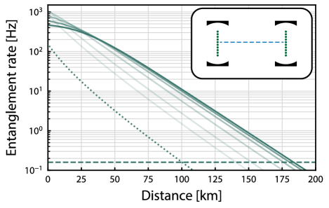
FIG. 4: Analysis of a single link. (a) Multiplexed entanglement generation between two nodes, each containing an array of atoms in an optical cavity. The mean entanglement distribution rate versus the length of the link for various numbers of atoms $N$ is shown as an opacity scale for $N=\{10,20,50,100,150,200\}$ with $N=200$ being fully opaque. This scale is used in subsequent figures. The dotted line shows the entanglement distribution rate for $N=1$. The horizontal dashed line shows a conservative estimate for the anticipated decoherence rate of the atoms. Here we focus on the rates associated with successfully generating a single Bell pair with one atom at each node (inset).

We compare the entanglement rate to the coherence time of the qubits in the nodes. We assume a conservative lower bound of $T_{2}=1\,\text{s}$ for our nuclear qubits, but note that it could approach the minute scale Young2020 . Hence, we consider distribution rates above $\Gamma_{\text{coherence}}=1/(2\pi T_{2})=0.16$ Hz to have a sufficiently high link efficiency Hucul2015 for useful entanglement. This criterion suggests that our platform will enable the generation of entanglement over $\approx 180\,\text{km}$ using $N=200$ atoms, which is well within the reach of current technology Ebadi2020 . For context, the current record for matter-based qubits is 1.3 km Hansen2015 .

V Entanglement distribution using quantum repeater nodes

We now turn to the use of intermediate repeater nodes to extend the range of entanglement generation to greater distances. The goal is to connect these intermediate links into a larger chain which we refer to as the “network-level” architecture. We break the length $L$ between end-users Alice and Bob into $2^{m}$ segments with length $L_{m}=L/2^{m}$, where $m$ is a non-negative integer we call the “nesting level” of the network.

V.1 Overview of the protocol

We divide the intermediate links into two groups in alternation such that adjacent links are not in the same group [see Fig. 5(a)]. Our protocol is based on the generation of Bell pairs across all Group 1 links in parallel followed by all Group 2 links in parallel. Naively, the mean time required to generate Bell pairs across all links is approximately twice the mean time required for a single link. However, the number of attempts required to successfully create entanglement follows a geometric distribution and both groups must wait for the success of all constituent links. Hence, we stochastically sample the distribution of attempts for each link in both groups in order to estimate mean entanglement generation rates at the network level (see Appendix D for details). Note that if $N$ atoms are employed in the multiplexed entanglement generation in Group 1, $N-1$ atoms are available for generating entanglement in Group 2.

After the Bell pairs have been generated on Group 1 links, the constituent atom at each node in these Bell pairs – recognized by its time stamp – must be isolated and preserved from the subsequent operations on the Group 2 links. Our protocol is based on transferring those qubits from the nuclear spin-$1/2$ ground state (${}^{1}\text{S}_{0}$) to an auxiliary computational basis Gorshkov2009 of the nuclear spin-$1/2$ metastable clock state (${}^{3}\text{P}_{0}$) that has a lifetime of $\approx 20\,\text{s}$. Accordingly, we leverage the (nearly-)clock-magic wavelength of the cavity standing wave-optical tweezer trap system. The metastable clock state is transparent with respect to the four-wave mixing sequence and a negligible relative phase is anticipated on this auxiliary qubit. We expect that transferring the qubit to the auxiliary basis will occur at a rate much faster than the entanglement generation rates over distances of interest and therefore have a negligible effect on the total rate. Rates of $\Omega_{\text{clock}}\approx 2\pi\times 100\,\text{kHz}$ and a transfer fidelity of $\gtrsim 0.99$ are anticipated with ${}^{171}\text{Yb}$ Young2020 . Alternatively, the atom(s) could be moved away from the array and the laser fields to preserve coherence during Group 2 operations.

FIG. 5: Network-level entanglement generation. (a) In order to distribute entanglement to end-users Alice and Bob over greater distances, $2^{m}-1$ intermediate repeater nodes are used, where $m$ is the nesting level. Bell pairs are generated in parallel within Group 1 (blue) and Group 2 (red). Intermediate nodes have two atoms involved in Bell pairs. (b) Simulated entanglement distribution rates over the full network versus the network length $L$ for nesting levels $m=2$ (blue), $3$ (orange), and $4$ (yellow) with number of atoms per node $N$ shown as the same opacity scale as in Fig. 4. The dashed lines again show conservative estimates of the coherence of the qubits at each nesting level. Note that the number of qubits depends on $m$, so the estimated coherence is $2^{m}/(2\pi T_{2})$. The black dotted line shows for comparison the direct entanglement distribution rate by sending entangled photon pairs at a rate of $10\,\text{GHz}$ Pirandola2017 .

With Bell pairs across all neighboring links, we now complete the end-to-end entanglement protocol by entangling atomic pairs and performing deterministic Bell-state measurements at each node to effectively reduce the nesting level of the network by 1. Bell pairs between increasingly distant nodes are traced out of the system through this process (see Appendix A) until end-users Alice and Bob directly share a Bell pair. We couple to highly-excited Rydberg states to perform the required local deterministic entanglement operations Levine2019 ; Graham2019 ; Madjarov2020 , inspired by a recent approach with alkaline-earth atoms coupling from the clock state to Rydberg states in the ${}^{3}\text{S}_{1}$ series Madjarov2020 . However, this interaction occurs only over short distances, requiring the atomic pairs to be re-positioned [see Fig. 1(c)]. The optical tweezers will remove the atoms from the cavity standing wave and translate them to within several microns of each other prior to Rydberg excitation. Tweezer-mediated coherent translation of atomic qubits over such distances is routinely performed on the $\sim\text{ms}$ timescale with minimal decoherence Beugnon2007 ; Lengwenus2010 ; Schymik2020 ; Dordevic2021 and Rydberg-mediated gates are on the $\lesssim\mu$s timescale Levine2019 ; Graham2019 ; Madjarov2020 . These steps are again much faster than the entanglement distribution rates and are only performed when remote Bell pairs have been successfully created, so we can neglect their effect on the total rate. The expected near-term fidelity of Rydberg-mediated gates and local measurement is $\gtrsim 0.99$ Covey2019 ; Madjarov2020 , which is high compared to the fidelity of generating Bell pairs: $\approx 0.98^{2}=0.96$ [see Fig. 3(d)]. A detailed network fidelity budget is outside the scope of this work.

V.2 Summary of the results

We consider the network-level entanglement distribution rate based on this protocol for varied network length $L$, nesting level $m$, and atom number per node $N$. We compare this rate against a conservative estimate of the coherence of all qubits in the system. Naturally, this depends on the nesting level, and hence the network level coherence estimate is $\Gamma_{\text{coherence}}^{m}=2^{m}/(2\pi T_{2})=0.16\times 2^{m}\,\text{Hz}$. Figure 5(b) shows the network level generation rate versus the network length for nesting levels $m=2,\,3,\,4$ with various atom numbers per node $N$ shown as an opacity scale. We also compare against direct communication (without intermediate nodes) based on entangled photon pairs at a wavelength of $1550\,\text{nm}$ with a repetition rate of $10\,\text{GHz}$ Pirandola2017 . The direct communication rate falls sharply, passing below our coherence time estimates at a distance of $\approx 600\,\text{km}$. We find that the achievable network length increases for higher nesting level and saturates for $N\approx 200$ atoms. In particular, for $m=4$ our system enables a network of $L\approx 1500\,\text{km}$.

VI Multiple Bell pairs and entanglement purification

We now consider the generation of multiple Bell pairs with our system, which are needed for more advanced protocols such as purification and logical encoding. Entanglement purification (also known as distillation) Dur2003 ; Bennett1996a ; Kalb2017 is based on taking two (or more) Bell pairs and consuming them to generate a single Bell pair with higher fidelity (See Appendix A). Purification requires entanglement operations between the local qubits in the pairs combined with single-qubit readout within each node. The former will again be accomplished with Rydberg-mediated gates Levine2019 ; Graham2019 ; Madjarov2020 while the latter will leverage the auxiliary qubit basis in the metastable clock state to perform single-atom readout by scattering photons from the ${}^{1}\text{S}_{0}\leftrightarrow{}^{3}\text{P}_{1}$ transition, to which the ${}^{3}\text{P}_{0}$ clock state is transparent Monz2016 ; Erhard2021 .

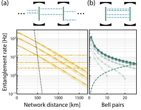
FIG. 6: Multiple Bell pairs at the network and single link levels. (a) The simulated entanglement distribution rate for $m=4$ versus network distance for one Bell pair (dot-dashed), two Bell pairs (dot-dot-dashed), and five Bell pairs (dot⁵-dashed) with $N=\{100,150,200\}$ as an opacity scale. The black dotted line is again direct communication at $10\,\text{GHz}$. The horizontal dashed lines are the expected coherence associated with the total number of qubits. For multiple Bell pairs $B>1$, this is $\Gamma_{\text{coherence}}^{m,B}=B\cdot 2^{m}/(2\pi T_{2})$. The maximum distance falls from $\approx 1500$ to $\approx 1100\,\text{km}$ when increasing the number of Bell pair from one to two. (b) The entanglement distribution rate of a single link with distance $L=50\,\text{km}$ to represent a metropolitan-scale network. The rate is plotted versus the number of Bell pairs with $N$ from 10 to 200 as an opacity scale. This shows a favorable scaling with $B$, and that $B=26$ Bell pairs can be generated with $N=200$, where the dashed line is again the expected coherence associated with the total number of qubits. Entanglement of $B>N$ pairs is impossible; hence rates for these data points are omitted.

To this end, we study the network-level entanglement generation rate versus network length $L$ with $m=4$ for various numbers of Bell pairs. We find that rate associated with generating $B$ Bell pairs in a given attempt decays exponentially with $B$; hence, we instead use a “ladder” scheme analogous to the network-level analysis. Specifically, we create $B$ Bell pairs one at a time on each link [see Fig. 6(a)], and still divide the links into two groups. Here again, we must sample the distribution of attempts before the successful generation of each Bell pair on each link, and both Group 1 and 2 are limited by the time for each constituent link to generate $B$ pairs.

We find that the simulated mean entanglement generation rate for $B=2$ exceeds the decoherence of the $B\cdot 2^{m}$ Bell pairs for distances up to $L\approx 1100\,\text{km}$. These findings indicate that our platform may be compatible with the development of a transcontinental terrestrial quantum network with sufficiently high fidelity – based on entanglement purification – for subsequent nontrivial operations. Interestingly, we find a favorable scaling with $B$ and include $B=5$ in Fig. 6(a), showing rates exceeding decoherence for distances up to $L\approx 500\,\text{km}$.

Finally, we consider the possibility of generating many Bell pairs over a metropolitan-scale link with $L=50$ km for advanced error correction protocols or for the distribution of many-body states such as logically-encoded qubits Fowler2012 ; Albert2020 ; Erhard2021 , atomic cluster or graph states Choi2019 , spin-squeezed states Polzik2016 ; Pezze2018 ; Pedrozo2021 or Greenberger-Horne-Zeilinger (GHZ) states Komar2014 ; Omran2019 . We analyze the entanglement generation rate versus the number of Bell pairs per link for various $N$ in Fig. 6(b). Crucially, we find that 26 Bell pairs can be generated for $N=200$ – comparable with the largest GHZ states created locally to date Omran2019 ; Song2019 ; Marciniak2021 – offering new opportunities for distributed computing and error-corrected networking.

VII Outlook and conclusion

We have proposed a platform that combines the strengths of neutral atoms – efficient light-matter interfaces McKeever2003 ; Birnbaum2005 ; Tiecke2014 ; Reiserer2015 with telecom operation Uphoff2016 ; Covey2019b ; Menon2020 , high-fidelity qubit operations and measurement Levine2019 ; Graham2019 ; Covey2019 ; Madjarov2020 , scalability to many qubits Bernien2017 ; Browaeys2020 ; Ebadi2020 , and long coherence times in state-independent optical traps Madjarov2019 ; Norcia2019 ; Young2020 – for the first time to enable new directions in quantum communication and distributed quantum computing. Moreover, we have demonstrated how this platform can offer dramatic improvements in entanglement generation rates over long distances by time-multiplexing across an array of atoms within each entanglement generation attempt.

We show that entanglement generation rates with $N\approx 100$ atoms across $\gtrsim 100\,\text{km}$-links compare favorably with conservative estimates of the atoms’ coherence time. We further demonstrate that multiplexed repeater-based networks with $2^{(m=4)}$ links and $N\approx 100$ atoms at each node can generate entanglement over $\approx 1500\,\text{km}$. Additionally, we show that our system is well-suited for entanglement purification Dur2003 ; Bennett1996a ; Kalb2017 and can achieve a purified network range to $\approx 1100\,\text{km}$, providing a promising architecture for a transcontinental quantum network. This network architecture is also compatible with heterogeneous hardware, and may be combined with microwave-to-optical transduction Covey2019c ; Lauk2020 to provide a robust network between superconducting quantum processors Arute2019 . Finally, we consider the prospects for generating larger numbers of Bell pairs for more advanced protocols such as distributing logically-encoded or other many-body states relevant for quantum computing and metrology. We find that $26$ Bell pairs can be generated over a metropolitan link of $50\,\text{km}$.

More generally, the confluence of the associated research thrusts – Rydberg atoms arrays Saffman2010 ; Browaeys2020 , cavity QED with strong atom-photon coupling McKeever2003 ; Birnbaum2005 ; Tiecke2014 , and atom-array optical clocks Madjarov2019 ; Norcia2019 ; Young2020 – into one platform will enable new methods to engineer, measure, and distribute many-body entangled states with single-qubit control. For example, the optical cavity can mediate non-demolition measurements Boca2004 ; Kalb2015 that could augment the Rydberg-based quantum computing platform. Conversely, Rydberg-mediated interactions and single-atom control may help to enhance and distribute spin-squeezed states of optical clock qubits generated via the cavity Polzik2016 ; Pezze2018 ; Pedrozo2021 . Finally, the marriage of short-ranged (Rydberg-mediated) and infinite-ranged (cavity-mediated) interactions combined with the possibility of atom-selective control and readout will enable new opportunities for the study of quantum many-body phenomena such as the simulation of magnetism Davis2019 and chaotic dynamics Choi2021 in regimes not readily accessible to classical computers.

APPENDIX A Quantum repeater and purification protocols

The repeater protocol Duan2001 ; Pirandola2019 is based on creating two Bell pairs, where end-users Alice and Bob each have half of one pair and the intermediate node has half of both. Then, the combination of a deterministic two-qubit controlled-NOT gate (CNOT), a single-qubit Hadamard gate, and the qubit measurements swaps the entanglement out of the two qubits at the intermediate node and leaves Alice and Bob’s halves entangled in a Bell pair with no quantum information remaining at the intermediate node [see Fig. S1(a)].

The purification protocol Dur2003 ; Bennett1996a ; Kalb2017 is based on creating two Bell pairs, where end-users Alice and Bob each have half of both pairs. A CNOT gate and a single-qubit measurement at both nodes leaves only one Bell pair between Alice and Bob that has higher fidelity than either initial pair. No quantum information remains in the other qubit pair [see Fig. S1(b)]. This protocol could be extended to the case of intermediate nodes and could be combined with the repeater protocol. We note that all necessary inner-node single- and two-qubit operations, and measurements for these protocols have been demonstrated in atomic arrays Levine2019 ; Graham2019 ; Madjarov2020 .

APPENDIX B Atomic and cavity QED parameters

1 Notes on the Yb telecom-band transitions

We begin this section by compiling a list of references for the Yb ${{}^{3}\text{P}_{J}\leftrightarrow{}^{3}\text{D}_{J^{\prime}}}$ transitions Bowers1996 ; Porsev1999 ; Loftus2002 ; Dzuba2010 ; Guo2010 ; Cho2012 ; Beloy2012 ; Lee2015 ; Antypas2019 . In the literature, there appears to be universal agreement that the decay rate from ${}^{3}\text{D}_{2}$ to ${}^{3}\text{P}_{1}$ (the transition of interest in this work) is $\Gamma_{{{}^{3}\text{D}_{2}\rightarrow{}^{3}\text{P}_{1}}}=2\times 10^{6}\,\text{s}^{-1}$ and the decay rate from ${}^{3}\text{D}_{2}$ to ${}^{3}\text{P}_{2}$ is $\Gamma_{{{}^{3}\text{D}_{2}\rightarrow{}^{3}\text{P}_{2}}}=2\times 10^{5}\,\text{s}^{-1}$. This corresponds to a branching ratio of the desired decay path of $0.87$.

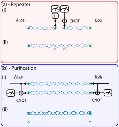
FIG. S1: Schematic overview of quantum repeater and purification protocols. See text for details.

However, there is disagreement about the decay rates of ${}^{3}\text{D}_{1}$ to ${}^{3}\text{P}_{J}$. In particular, the literature is split between $\{\Gamma_{{}^{3}\text{D}_{1}\rightarrow{}^{3}\text{P}_{0}},\Gamma_{{}^{3}\text{D}_{1}\rightarrow{}^{3}\text{P}_{1}},\Gamma_{{}^{3}\text{D}_{1}\rightarrow{}^{3}\text{P}_{2}}\}=\{200,100,3\}\times 10^{4}$ Bowers1996 ; Porsev1999 and $\{200,10,3\}\times 10^{4}\,\text{s}^{-1}$ Loftus2002 . We believe that Ref. Loftus2002 – which came after Refs. Bowers1996 ; Porsev1999 – introduced an error that has since propagated in the community. References Cho2012 ; Lee2015 ; Covey2019b ; Covey2019c have propagated this error, though it has not affected their arguments or conclusions, while Refs. Antypas2019 and others use the correct values.

2 Cavity QED parameters

We consider a cavity characterized by two parameters: the radius of curvature $R=5\,\text{mm}$ of its two mirrors and the length $\ell=9.75\,\text{mm}$ between them. For these parameters, the cavity is near-concentric, and satisfies the stability condition $0\leq\mathcal{G}^{2}\leq 1$, where $\mathcal{G}=1-\ell/R$ is the cavity stability parameter. We also characterize the principal mode of the cavity by its waist $w_{0}$, Rayleigh range $z_{0}$, and volume $V_{m}$ using

$$w_{0} =\left[\left(\frac{\lambda_{{}^{3}\text{D}_{2}\rightarrow{}^{3}\text{P}_{1}}\ell}{2\pi}\right)^{2}\left(\frac{1+\mathcal{G}}{1-\mathcal{G}}\right)\right]^{1/4},$$ (1)

$$z_{0} =\frac{\pi w_{0}^{2}}{\lambda_{{}^{3}\text{D}_{2}\rightarrow{}^{3}\text{P}_{1}}},$$ (2)

$$V_{m} =\frac{\pi}{4}w_{0}^{2}\ell,$$ (3)

where $\lambda_{{}^{3}\text{D}_{2}\rightarrow{}^{3}\text{P}_{1}}$ is the wavelength of the targeted telecom transition, $1480\,\text{nm}$. We also assume the cavity to have intrinsic finesse $F_{\text{int}}=10^{5}$, transmission linewidth $\kappa_{\text{int}}=2\pi\times c/2\ell F_{\text{int}}\approx 2\pi\times 154\,\text{kHz}$, and free spectral range $\text{FSR}=c/2\ell\approx 15.4\,\text{GHz}$. For a chosen extrinsic finesse $F_{\text{ext}}=5\times 10^{4}$ ($\kappa_{\text{ext}}\approx 2\pi\times 307\,\text{kHz}$), this gives a photon collection efficiency of $\eta_{\text{coll}}=1-F_{\text{ext}}/F_{\text{int}}=0.5$. Now we consider the atom-cavity interaction parameters essential to the proposed scheme. The electric dipole matrix element $D$ for our chosen transition is

$$\begin{split}D=\Bigg{[}&\frac{3\pi\varepsilon_{0}\hbar c^{3}}{\omega_{{}^{3}\text{D}_{2}\rightarrow{}^{3}\text{P}_{1}}^{3}}\Gamma_{{}^{3}\text{D}_{2}\rightarrow{}^{3}\text{P}_{1}}\\ &\phantom{\times}\begin{Bmatrix}J&J^{\prime}&1\\ F^{\prime}&F&I\end{Bmatrix}(2F^{\prime}+1)(2J^{\prime}+1)\Bigg{]}^{1/2},\end{split}$$ (4)

where $\omega_{{}^{3}\text{D}_{2}\rightarrow{}^{3}\text{P}_{1}}\approx 2\pi\times 202\,\text{THz}$, $\Gamma_{{}^{3}\text{D}_{2}\rightarrow{}^{3}\text{P}_{1}}=2\pi\times 318\,\text{kHz}$ and the term in braces is the Wigner 6-$j$ symbol, giving $D\approx 1.96\times 10^{-29}\,\text{C\,m}$. Using this, the coherent coupling to the cavity mode is

$$g_{34}=\frac{D}{\hbar}\left[\frac{\hbar\omega_{{}^{3}\text{D}_{2}\rightarrow{}^{3}\text{P}_{1}}}{2\varepsilon_{0}V_{m}}\right]^{1/2}\approx 2\pi\times 1.53\,\text{MHz},$$ (5)

which gives cooperativity $C=g_{34}^{2}/\kappa\Gamma_{{}^{3}\text{D}_{2}\rightarrow{}^{3}\text{P}_{1}}\approx 16.0$ with $\kappa=\kappa_{\text{int}}+\kappa_{\text{ext}}$. Then the probability of emitting a telecom photon into the cavity mode is $P_{\text{cavity}}=C/(C+1)\approx 0.941$, and hence the probability of extracting this photon for use in our scheme is $\eta_{\text{extract}}=P_{\text{cavity}}\eta_{\text{coll}}\approx 0.471$.

APPENDIX C Four-wave mixing

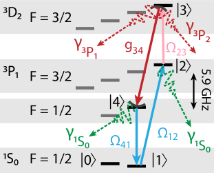
FIG. S2: Relevant levels of four-wave mixing. States ${|0\rangle}$ to ${|4\rangle}$ were considered for the simulation to estimate the success probability and fidelity. During the excitation cycle, the population in the levels ${|2\rangle}$ and ${|4\rangle}$ decay to state ${}^{1}\text{S}_{0}$ with a decay rate $\gamma_{{}^{1}\text{S}_{0}}=2\pi\times 182\,\text{kHz}$, and population in state ${|3\rangle}$ decays to state ${}^{3}\text{P}_{1}$ and ${}^{3}\text{P}_{2}$ with decay rate $\gamma_{{}^{3}\text{P}_{1}}=2\pi\times 318\,\text{kHz}$ and $\gamma_{{}^{3}\text{P}_{2}}=2\pi\times 48\,\text{kHz}$, respectively. For simulation purposes, all decays are assumed to accumulate in a dump level that does not contribute to the coherent evolution.

1 Numerical model and results

The atom-telecom photon entanglement generation protocol is similar to the four-level scheme previously shown for rubidium and cesium atoms coupled to nanophotonic cavities Menon2020 . The protocol starts with initializing atom in the superposition state $({|0\rangle}_{a}+{|1\rangle}_{a})/\sqrt{2}$. This is followed by a pulse sequence that takes the atom through states ${|1\rangle}\rightarrow{|4\rangle}$ before returning back to the initial state ${|1\rangle}$. First, pulse $\Omega_{12}$ transfers population from state ${|1\rangle}$ to ${|2\rangle}$. Then the population is excited to state ${|3\rangle}$ by light field $\Omega_{23}$, which is always on. The population that reaches the state ${|3\rangle}$ is preferentially transferred to state ${|4\rangle}$ via the emission of a telecom photon into the cavity, which is resonant with the ${|3\rangle}\leftrightarrow{|4\rangle}$ transition. A second pulse, $\Omega_{41}$, then transfers the population in the state ${|4\rangle}$ back to state ${|1\rangle}$. The spontaneous decay from excited states (see Fig. S2) limit the coherent completion of this cycle and leads to infidelities. Here we define the fidelity as the probability of finding the atom in the qubit state after the round-trip through states ${|1\rangle}\rightarrow{|4\rangle}$, given the heralding of the telecom photon.

The requirement of heralding makes this scheme robust to any atomic decays preceding the photon emission into the cavity and limits the infidelities to decays from the state ${|4\rangle}$. The optimum parameters for the given pulse sequence are extracted using a two-step optimization process Menon2020 . The first step optimizes the Rabi frequencies $\Omega_{12},\,\Omega_{23}$ and the pulse width of $\Omega_{12}$ to maximize the population transfer to the state ${|4\rangle}$ and the second step optimizes the timing, pulse width, and Rabi frequency of $\Omega_{41}$. In both the schemes below, the success probability accounts for the probability $P_{|1\rangle}$ for the initial population in ${|1\rangle}$ to emit a telecom photon and return to ${|1\rangle}$, as well as the probability for the emitted photon to couple to the external coupling mode of the cavity; i.e.

$$\text{Success probability}=\frac{\kappa_{\text{ext}}}{\kappa_{\text{int}}}P_{|1\rangle}$$ (6)

1.1 Resonant case

In the first case, which we call the “resonant case,” we have the cavity on resonant with the ${|3\rangle}\leftrightarrow{|4\rangle}$ transition. In this case the corresponding Hamiltonian in an appropriately chosen rotating frame is

$$\begin{split}\hat{H}&=\Omega_{12}(t){|1\rangle}{\langle 2|}+\Omega_{12}{|2\rangle}{\langle 3|}+g_{34}\hat{a}{|3\rangle}{\langle 4|}\\ &\phantom{=}+\Omega_{41}(t){|4\rangle}{\langle 1|}+\text{H.c.}\end{split}$$ (7)

In this resonant excitation scheme, the population transfer to ${|4\rangle}$ occurs over a time scale that is inversely proportional to atom-cavity coupling $g_{34}$, and for efficient completion, the second pulse has to be timed to match. The earlier coherent transfer spend a longer time in ${|4\rangle}$ leading to spontaneous decay. To minimize the contribution to infidelity, we transfer the population from ${|4\rangle}$ at earlier times, trading fidelity gains for reduced efficiency, due to incomplete population transfer. Here we achieve this by applying $\Omega_{41}$ earlier than what is optimal for the complete population transfer shown in Fig. 3(c). The increase in fidelity and corresponding reduction in the efficiency are shown in Fig.3(d). Fixed Gaussian pulses with full widths at half maximum $116\,\text{ns}$ and $58\,\text{ns}$ were used for $\Omega_{12}$ and $\Omega_{41}$, respectively. Here, the achieved fidelities were conditioned on heralding entanglement using the photons that were emitted until the coherent transfer back to the initial qubit state by $\Omega_{41}$. Detection of photons emitted from the cavity after the completion of $\Omega_{41}$ leads to additional infidelities.

FIG. S3: Detuned four-wave mixing scheme. (a) Time evolution of the coherent population in the states ${|1\rangle}$ to ${|4\rangle}$ and the photon emitted from the cavity through external coupling parameter $\kappa_{\text{ext}}$. The top half of the plot shows pulses $\Omega_{12}$ and $\Omega_{41}$. In the simulation, the first pulse is assumed to have a constant length of $65\,\text{ns}$ and the length of the second pulse is optimized for each value of the detuning. Here, both pulses have a $20\,\text{ns}$ ramp time. (b) Scaling of fidelity and success probability with detuning. Larger detuning leads to lower occupation and decay from state ${|4\rangle}$ at the cost of lower coherent population transfer back to state ${|1\rangle}$.

1.2 Detuned case

High-fidelity atom-telecom photon entanglement can also be obtained by using an off-resonant scheme, where the population transfer to ${|4\rangle}$ is minimized, since decay from this state is the dominant error in the heralding protocol. In this case the Hamiltonian considered is

$$\begin{split}\hat{H}&=\Omega_{12}(t){|1\rangle}{\langle 2|}+\Omega_{23}{|2\rangle}{\langle 3|}+g_{34}\hat{a}{|3\rangle}{\langle 4|}+\Omega_{41}(t){|4\rangle}{\langle 1|}\\ &\phantom{=}+\delta{|4\rangle}{\langle 4|}+\text{H.c.}\end{split}$$ (8)

In this scheme, the optimal fidelities were also found by a two-step optimization procedure. For a given detuning, the first step maximized the population transfer to ${|3\rangle}$ by optimizing the Rabi frequencies $\Omega_{12},\,\Omega_{23}$ and the pulse width of $\Omega_{12}$, and the second step optimizes the duration and Rabi frequency of $\Omega_{41}$ to maximize the population transfer from ${|3\rangle}$ to ${|1\rangle}$ through the two-photon process. Here, we fix the pulse length of $\Omega_{12}$ to $65\,\text{ns}$ including a linear ramp time of $20\,\text{ns}$. The length of $\Omega_{41}$ varies from $300\,\text{ns}$ to $500\,\text{ns}$ according to the varied detuning. Similar to the resonant case we again find that higher fidelities can be obtained at the cost of lower success probabilities [see Fig. S3(b)]. Incomplete population transfer in both schemes will lead to some residual population left behind in the states that are coupled to the cavity, which can lead to photon emission even after the end of the pulse sequence. Detection of these photons will add to infidelity. Overall success probabilities were found to be greater for the resonant scheme that is used in the main text for our calculations.

2 Phase matching considerations

We consider the importance of phase matching and momentum conservation of the four light fields that have overlapping amplitude during our four-wave scheme. We perform a qualitative estimate based on classical four-wave mixing analysis in which an outgoing wave is produced by the interaction of three incoming waves with a nonlinear medium Ender1982 . The outgoing field intensity is proportional to a phase-matching factor whose argument is $\xi=\Delta k\times L$, where $\Delta k=|\vec{k}_{12}+\vec{k}_{23}-\vec{k}_{34}-\vec{k}_{41}|$ and $L$ is the effective overlap length of the four fields which in practice is determined by their size or the size of the medium (whichever is smaller). The phase matching factor is equal to one when $\xi=0$ and decreases for $\xi\gg 0$.

For the beam configuration shown in Fig. 3(b) assuming a $180^{\circ}$ angle between $\vec{k}_{12}$ and $\vec{k}_{41}$ and a $45^{\circ}$ angle between $\vec{k}_{34}$ and $\vec{k}_{23}$, we estimate that $\Delta k\approx 2\pi/(1500\sqrt{2})\,\text{nm}$. The relevant length scale of the single-atom case should be the size of the atomic wavefunction in the optical trap, which we assume is $L_{\text{single}}\approx 50\,\text{nm}$. Hence, we estimate that $\xi<1$ for the case we consider here, so phase matching of the four light fields is not crucial. We therefore neglect it in our analysis, but choose a beam geometry to minimize $\Delta k$.

For an atomic ensemble or a solid-state spin ensemble, this factor would be much higher. Assuming $L=10\leavevmode\nobreak\ \mu$m with the same beam geometry, $\xi\gg 10$. Hence, phase matching is often crucial in ensemble and crystalline environments.

APPENDIX D Entanglement distribution calculations

We start by considering the rate $\Gamma_{\text{link}}$ at which entanglement between two adjacent network nodes can be attempted. This rate comprises all components shown in Fig. 2. The time to cool and initialize all atoms at the nodes (shown in blue in Fig. 2), performed globally and in parallel over the arrays of atoms at both nodes, is $1/\Gamma_{\text{init}}=1/10\,\text{kHz}$. This is based on the maximum scattering rate from the ³P₁ ($\Gamma_{{}^{3}\text{P}_{1}}\approx 90$ kHz) and an assumption about the number of photons required for cooling and optical pumping. The total qubit pulse time comprising globally applied $\pi/2$- and $\pi$-pulses (all time windows shown in green in Fig. 2) is $1/\Gamma_{\pi/2}+1/\Gamma_{\pi}=3/\Gamma_{\pi/2}=3/100\,\text{kHz}$, based on an assumed Rabi frequency of 50 kHz via stimulated Raman pulses between the nuclear spin states. The total four-wave-mixing time (shown in orange in Fig. 2) is $2N/\Gamma_{\text{FWM}}=2N/200\,\text{kHz}$ for all $N$ atoms. The four-wave-mixing rate is determined by the time between when the sequence begins and when the photon leaves the cavity with high probability [see Fig. 3(c)]. Finally, the time to transmit classical signals through fibers and to herald entanglement (shown in purple in Fig. 2) is $1/\Gamma_{\text{comm}}(L)=c/2L\approx 10^{8}\,\text{m\,s${}^{-1}$}/L$.

Table S1: Rates for constituent steps in the single-link multiplexing protocol. Exact values for rates composing the total rate at which entanglement between two adjacent network nodes $\Gamma_{\text{link}}$ can be attempted (Eq. 12) in terms of the per-node atom number $N$ and distance in fiber between nodes $L$. The listed steps correspond chronologically to the colored time windows shown in Fig. 2(a) and (b).

Step	Symbol	Description	Global?	Rate [kHz]
1	$\Gamma_{\text{init}}$	Optical pumping and cooling	Global	$10$
2	$\Gamma_{\pi/2}$	$\pi/2$-pulse	Global	$100$
3	$\Gamma_{\text{FWM}}$	FWM protocol	One-by-one	$200/N$
4	$\Gamma_{\pi}$	$\pi$-pulse	Global	$50$
5	$\Gamma_{\text{FWM}}$	FWM protocol	Global (same order)	$200/N$
6	$\Gamma_{\text{comm}}(L)$	Heralded entanglement	Global (atom-unique time stamp)	$c/2L$

Using these quantities, $\Gamma_{\text{link}}$ is

$$\Gamma_{\text{link}}(L,N)=\left[\frac{1}{\Gamma_{\text{init}}}+\frac{3}{\Gamma_{\pi/2}}+\frac{2N}{\Gamma_{\text{FWM}}}+\frac{1}{\Gamma_{\text{comm}}(L)}\right]^{-1}.$$ (9)

The exact values used for these rates are summarized in Table S1.

The probability $p$ of successfully creating a single Bell pair between any given two atoms at adjacent nodes similarly comprises several components;

$$p(L)=\left(\frac{1}{2}\right)^{2}\eta_{\text{FWM}}^{2}\,\eta_{\text{fiber}}^{2}\,\eta_{\text{det}}^{2}\,\eta_{\text{att}}(L).$$ (10)

Here, $\eta_{\text{FWM}}\approx 0.364$ is the total success probability of the four-wave-mixing scheme under the condition shown in Fig. 3(d); $\eta_{\text{fiber}}=\eta_{\text{det}}=0.9$ are the efficiencies at which photons may be collected by their respective fibers and subsequently detected; and $\eta_{\text{att}}(L)=\exp(-L/\lambda_{\text{att}})$ is the attenuation of the telecom photons ($\lambda_{\text{att}}=20.7\,\text{km}$ at $1480\,\text{nm}$ Corning2020 ). The two leading factors of $1/2$ are due to the overlap between the Bell-state and computational bases and an assumed complete loss of photon polarization in the long-distance fibers. It follows that the total probability $P_{\text{mux}}$ of creating at least $B$ Bell pairs between adjacent nodes through multiplexing is

$$P_{\text{mux}}(L,N,B)=\sum\limits_{k=B}^{N}\binom{N}{k}p^{k}(1-p)^{N-k}$$ (11)

for $N\geq B$ and zero otherwise.

To calculate the rate $\Gamma_{\text{mux}}$ at which these $B$ or more Bell pairs can be formed between atoms at adjacent network nodes, we consider a total number of times $M$ that the entire procedure is attempted. While $M$ is in principle unbounded, it is realistic to choose $M$ such that the mean number of successful attempts $MP_{\text{mux}}(L,N,B)$ to create $\geq B$ Bell pairs is one, and hence the average success rate is that at which these $M$ attempts can be performed,

$$\Gamma_{\text{mux}}(L,N,B)=\Gamma_{\text{link}}(L,N)\times P_{\text{mux}}(L,N,B).$$ (12)

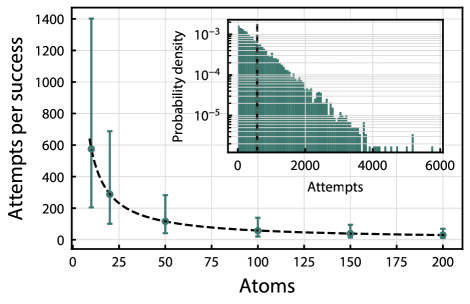
FIG. S4: Comparison of simulation with Eq. 11. The simulated mean number of attempts $M$ required for the formation of one Bell pair across a single link for various $N$ at $L=100\,\text{km}$ (green circles), averaged over $10,000$ trials, are compared in the main plot with the expected analytically derived result $M=1/P_{\text{mux}}$ (black dashed line). The error bars show the one-sided RMS deviation from the mean. The inset shows the distribution over values of $M$ associated with the $N=10$ data point along with the mean of the distribution (gray dotted line) and analytical result (black dashed line).

Generalizing to the network-level procedure, the two-group structure [see Sec. V] requires an extra consideration. The proposed protocol requires that entanglements in Group 1 complete before those in Group 2 can be attempted, which precludes the derivation of an analytical formula to describe the expected rates; hence we turn to numerical simulation to calculate the results shown in Figs. 5 and 6. We use a simple simulation scheme based on stochastically sampling the probability distribution over $M$ attempts required for the formation of Bell pairs across each network link in accordance with Eq. 11, which gives $M=1/P_{\text{mux}}$ for one success across a link for given $N$, $L$, and $B$. For our simulations, $M$ – which follows a geometric distribution – is sampled by counting the number of random events required for a single success, which occurs with probability $P_{\text{mux}}$. The resulting averages of these counts over $10,000$ trials are in good agreement with the expected value obtained using Eq. 11, shown in Fig. S4. The time taken for each linking attempt is then $M/\Gamma_{\text{link}}$, and the mean of a set of $Q$ such trials can be inverted to find the average entanglement rate. It was found that this scheme could be used for as few as $Q=1000$ trials to faithfully reproduce Fig. 4.

At the network level, the results shown in Figs. 5 and 6(a) were calculated following the two-group protocol as described. The single-link linking time $M/\Gamma_{\text{link}}$ was singly sampled for each of the $2^{m-1}$ network links in Group 1, from which the maximum was selected. This sampling was repeated for $2^{m-1}$ links in Group 2 (for $N-1$ atoms at each node), and the two maxima were added to find the total time required for the network. The mean of $Q=5000$ such trials was then inverted to calculate the average rate for each value of $m$, $N$, and $L$ shown. For the multi-Bell case shown in Fig. 6(b), the single single-link procedure described in the previous paragraph was repeated for $B$ Bell pairs following the “ladder” scheme [see Sec. VI], the total time for $B$ linking attempts averaged over $Q=5000$ trials, and the average inverted for each value of $N$ and $B$ shown.

References

- (1) J. I. Cirac, P. Zoller, H. J. Kimble, and H. Mabuchi, Phys. Rev. Lett. 78, 3221 (1997).
- (2) S. Wehner, D. Elkouss, and R. Hanson, Science 362, eaam9288 (2018).
- (3) H. J. Kimble, Nature 453, 1023 (2008).
- (4) S. Pirandola et al., Adv. Opt. Photonics 12, 1012 (2020).
- (5) L. Jiang, J. M. Taylor, A. S. Sørensen, and M. D. Lukin, Phys. Rev. A 76, 062323 (2007).
- (6) P. Kómár et al., Nat. Phys. 10, 582 (2014).
- (7) A. W. Young et al., Nature 588, 408 (2020).
- (8) S. Ebadi et al., Nature 595, 227 (2021).
- (9) M. Saffman, T. G. Walker, and K. Mølmer, Rev. Mod. Phys. 82, 2313 (2010).
- (10) H. Levine et al., Phys. Rev. Lett. 123, 170503 (2019).
- (11) T. M. Graham et al., Phys. Rev. Lett. 123, 230501 (2019).
- (12) M. Uphoff, M. Brekenfeld, G. Rempe, and S. Ritter, Appl. Phys. B 122, 46 (2016).
- (13) J. P. Covey et al., Phys. Rev. Appl. 11, 034044 (2019).
- (14) S. G. Menon, K. Singh, J. Borregaard, and H. Bernien, New J. Phys. 22, 073033 (2020).
- (15) A. Reiserer and G. Rempe, Rev. Mod. Phys. 87, 1379 (2015).
- (16) S. Ritter et al., Nature 484, 195 (2012).
- (17) J. Hofmann et al., Science 337, 72 (2012).
- (18) P. Samutpraphoot et al., Phys. Rev. Lett. 124, 063602 (2020).
- (19) S. Langenfeld et al., Phys. Rev. Lett. 126, 130502 (2021).
- (20) S. Daiss et al., Science 371, 614 (2021).
- (21) T. Dordević et al., arXiv Prepr. 2105.06485 (2021).
- (22) L.-M. Duan, M. D. Lukin, J. I. Cirac, and P. Zoller, Nature 414, 413 (2001).
- (23) W. Pfaff et al., Nat. Phys. 9, 29 (2013).
- (24) T. M. Graham, J. T. Barreiro, M. Mohseni, and P. G. Kwiat, Phys. Rev. Lett. 110, 060404 (2013).
- (25) N. Sinclair et al., Phys. Rev. Lett. 113, 053603 (2014).
- (26) F. Kaneda et al., Optica 2, 1010 (2015).
- (27) T. Zhong et al., Science 357, 1392 (2017).
- (28) S. Wengerowsky, S. K. Joshi, F. Steinlechner, H. Hübel, and R. Ursin, Nature 564, 225 (2018).
- (29) Corning SMF-28 Ultra Opt. Fiber , https://www.corning.com/.
- (30) W. Dür and H.-J. Briegel, Phys. Rev. Lett. 90, 067901 (2003).
- (31) C. H. Bennett et al., Phys. Rev. Lett. 76, 722 (1996).
- (32) N. Kalb et al., Science 356, 928 (2017).
- (33) S. D. Barrett and P. Kok, Phys. Rev. A 71, 060310 (2005).
- (34) H. Bernien et al., Nature 497, 86 (2013).
- (35) M. Endres et al., Science 354, 1024 (2016).
- (36) D. Barredo, S. de Léséleuc, V. Lienhard, T. Lahaye, and A. Browaeys, Science 354, 1021 (2016).
- (37) A. Cooper et al., Phys. Rev. X 8, 041055 (2018).
- (38) M. A. Norcia, A. W. Young, and A. M. Kaufman, Phys. Rev. X 8, 041054 (2018).
- (39) S. Saskin, J. T. Wilson, B. Grinkemeyer, and J. D. Thompson, Phys. Rev. Lett. 122, 143002 (2019).
- (40) B. Casabone et al., Phys. Rev. Lett. 111, 100505 (2013).
- (41) C. H. Nguyen, A. N. Utama, N. Lewty, and C. Kurtsiefer, Phys. Rev. A 98, 063833 (2018).
- (42) E. J. Davis, G. Bentsen, L. Homeier, T. Li, and M. H. Schleier-Smith, Phys. Rev. Lett. 122, 010405 (2019).
- (43) J. Zeiher, J. Wolf, J. A. Isaacs, J. Kohler, and D. M. Stamper-Kurn, arXiv Prepr. 2012.01280 (2020).
- (44) J. P. Covey, A. Sipahigil, and M. Saffman, Phys. Rev. A 100, 012307 (2019).
- (45) J. P. Covey, I. S. Madjarov, A. Cooper, and M. Endres, Phys. Rev. Lett. 122, 173201 (2019).
- (46) M. A. Norcia et al., Science 366, 93 (2019).
- (47) I. S. Madjarov et al., Phys. Rev. X 9, 041052 (2019).
- (48) I. S. Madjarov et al., Nat. Phys. 16, 857 (2020).
- (49) J. Wilson et al., arXiv Prepr. 1912.08754 (2019).
- (50) E. S. Polzik and J. Ye, Phys. Rev. A 93, 021404 (2016).
- (51) H. Bernien et al., Nature 551, 579 (2017).
- (52) J. Choi et al., arXiv Prepr. 2103.03535 (2021).
- (53) A. Browaeys and T. Lahaye, Nat. Phys. 16, 132 (2020).
- (54) J. McKeever, A. Boca, A. D. Boozer, J. R. Buck, and H. J. Kimble, Nature 425, 268 (2003).
- (55) K. M. Birnbaum et al., Nature 436, 87 (2005).
- (56) T. G. Tiecke et al., Nature 508, 241 (2014).
- (57) D. Hunger et al., New J. Phys. 12, 065038 (2010).
- (58) F. Haas, J. Volz, R. Gehr, J. Reichel, and J. Esteve, Science 344, 180 (2014).
- (59) M. Brekenfeld, D. Niemietz, J. D. Christesen, and G. Rempe, Nat. Phys. 16, 647 (2020).
- (60) J. A. Sedlacek et al., Phys. Rev. Lett. 116, 133201 (2016).
- (61) T. Thiele et al., Phys. Rev. A 92, 063425 (2015).
- (62) M. Teller et al., Phys. Rev. Lett. 126, 230505 (2021).
- (63) A. Kawasaki et al., Phys. Rev. A 99, 013437 (2019).
- (64) J. Ye, H. J. Kimble, and H. Katori, Science 320, 1734 (2008).
- (65) D. Hucul et al., Nat. Phys. 11, 37 (2015).
- (66) B. Hensen et al., Nature 526, 682 (2015).
- (67) A. V. Gorshkov et al., Phys. Rev. Lett. 102, 110503 (2009).
- (68) S. Pirandola, R. Laurenza, C. Ottaviani, and L. Banchi, Nat. Commun. 8, 15043 (2017).
- (69) J. Beugnon et al., Nat. Phys. 3, 696 (2007).
- (70) A. Lengwenus, J. Kruse, M. Schlosser, S. Tichelmann, and G. Birkl, Phys. Rev. Lett. 105, 170502 (2010).
- (71) K.-N. Schymik et al., Phys. Rev. A 102, 063107 (2020).
- (72) T. Monz et al., Science 351, 1068 (2016).
- (73) A. Erhard et al., Nature 589, 220 (2021).
- (74) A. G. Fowler, M. Mariantoni, J. M. Martinis, and A. N. Cleland, Phys. Rev. A 86, 032324 (2012).
- (75) V. V. Albert, J. P. Covey, and J. Preskill, Phys. Rev. X 10, 031050 (2020).
- (76) H. Choi, M. Pant, S. Guha, and D. Englund, npj Quantum Inf. 5, 104 (2019).
- (77) L. Pezzè, A. Smerzi, M. K. Oberthaler, R. Schmied, and P. Treutlein, Rev. Mod. Phys. 90, 035005 (2018).
- (78) E. Pedrozo-Peñafiel et al., Nature 588, 414 (2020).
- (79) A. Omran et al., Science 365, 570 (2019).
- (80) C. Song et al., Science 365, 574 (2019).
- (81) C. D. Marciniak et al., arXiv Prepr. 2107.01860 (2021).
- (82) N. Lauk et al., Quantum Sci. Technol. 5, 020501 (2020).
- (83) F. Arute et al., Nature 574, 505 (2019).
- (84) A. Boca et al., Phys. Rev. Lett. 93, 233603 (2004).
- (85) N. Kalb, A. Reiserer, S. Ritter, and G. Rempe, Phys. Rev. Lett. 114, 220501 (2015).
- (86) C. J. Bowers et al., Phys. Rev. A 53, 3103 (1996).
- (87) S. G. Porsev, Y. G. Rakhlina, and M. G. Kozlov, Phys. Rev. A 60, 2781 (1999).
- (88) T. Loftus, J. R. Bochinski, and T. W. Mossberg, Phys. Rev. A 66, 013411 (2002).
- (89) V. A. Dzuba and A. Derevianko, J. Phys. B At. Mol. Opt. Phys. 43, 074011 (2010).
- (90) K. Guo, G. Wang, and A. Ye, J. Phys. B At. Mol. Opt. Phys. 43, 135004 (2010).
- (91) J. W. Cho et al., Phys. Rev. A 85, 035401 (2012).
- (92) K. Beloy et al., Phys. Rev. A 86, 051404 (2012).
- (93) J. Lee, J. H. Lee, J. Noh, and J. Mun, Phys. Rev. A 91, 053405 (2015).
- (94) D. Antypas et al., Nat. Phys. 15, 120 (2019).
- (95) D. A. Ender, Doubly-Resonant Two-Photon-Absorption-Induced Four-Wave Mixing in Tb(OH)3 and LiTbF4, Ph.d. thesis, Montana State University, 1982.