Characterizing the surface texture of a dense suspension undergoing dynamic jamming

Abstract

Measurements of the surface velocity and surface texture of a freely propagating shear jamming front in a dense suspension are compared. The velocity fields are captured with particle image velocimetry (PIV), while the surface texture is captured in a separated experiment by observing a direct reflection on the suspension surface with high-speed cameras. A method for quantifying the surface features and their orientation is presented based on the fast Fourier transform of localised windows. The region that exhibits strong surface features corresponds to the the solid-like jammed region identified via the PIV measurements. Moreover, the surface features within the jammed region are predominantly oriented in the same direction as the eigenvectors of the strain tensor. Thus, from images of the free surface, our analysis is able to show that the surface texture contains information on the principle strain directions and the propagation of the jamming front.

1 Introduction

Suspensions of hard spheres in a Newtonian fluid are known to jam at a critical volume fraction (Krieger, 1972). That is, beyond a critical concentration of particles, flow ceases and a finite yield stress is observed Brown and Jaeger (2014). However, for some suspensions, such as cornstarch and water, a jammed state is accessible for volume fractions lower than the critical volume fraction when stress is applied (Wyart and Cates, 2014; Peters et al, 2016). This rather counter intuitive phenomenon is called dynamic jamming or shear jamming, where the suspension appears fluid-like at low stress, but shear thickens and even jams with sufficiently high stress. As such, a sudden impact causes the suspension to jam (Waitukaitis and Jaeger, 2012; Jerome et al, 2016), which explains how it is possible to stay afloat while running over a cornstarch suspension (Mukhopadhyay et al, 2018; Baumgarten and Kamrin, 2019).

The assumption of smooth, force free particles in non-Brownian, non-inertial systems, where viscosity is only a function of the volume fraction, $\phi$ (Stickel and Powell, 2005), does not capture this behaviour. In real suspensions particle-particle interactions are an important contributor to the observed behaviour (Lin et al, 2015; Gadala‐Maria and Acrivos, 1980; Brown and Jaeger, 2014). Between particles, it has been identified that friction (Mari et al, 2014; Singh et al, 2018; Sivadasan et al, 2019; Tapia et al, 2019; Madraki et al, 2017; Fernandez et al, 2013) and repulsive forces (Brown and Jaeger, 2014; James et al, 2018; Guy et al, 2015) are underlying mechanisms for understanding this phenomenon. With a sufficient amount of applied stress, the particles overcome the repulsive force, and are brought into frictional contact. At sufficiently high particle concentrations, the contacts form a network capable of supporting the applied stresses.

In sufficiently large domains, the transition from fluid-like to solid-like is observed as a front of high shear rate that propagates from the perturbing body through the suspension and leaves a jammed state in its wake (Waitukaitis and Jaeger, 2012; Peters and Jaeger, 2014; Han et al, 2016; Peters et al, 2016; Majumdar et al, 2017; Han et al, 2018, 2019b; Baumgarten and Kamrin, 2019; Rømcke et al, 2021). In these works, the jamming front is defined by the velocity contour at half the velocity of the perturbing body, i.e., $0.5U_{c}$. A normalized front propagation factor is used to quantify how fast the front moves, defined by the relation between the speed of the $0.5U_{c}$-contour and the perturbing body. The front propagation factor is observed to increase with volume fraction and is independent of perturbing speed for sufficiently high velocities (Han et al, 2016; Rømcke et al, 2021). This phenomenology is caused by an intrinsic strain (Han et al, 2019a; Baumgarten and Kamrin, 2019) which is needed in order for the material to build a frictional contact network capable of supporting the applied stresses. The strain level decreases with increasing volume fraction and has an inverse relationship with the front propagation factor (Han et al, 2019a).

Most measurement set-ups employed to investigate this problem have a free surface, and as such, the effects of the free surface have been identified as an important question in suspension flow (Denn et al, 2018). One interesting feature is the existence of two statically stable states (Cates et al, 2005; Cates and Wyart, 2014) known as granulation. The material can exist as a flowable droplet with a shiny surface, or in a stressed state as a jammed, pasty granule upheld by capillary forces. A closely linked observable surface feature in dense suspension flow is dilation (Brown and Jaeger, 2012; Jerome et al, 2016; Maharjan et al, 2021). For a sufficiently dense suspension, the granular structure expands under shear, which sets up a suction in the liquid phase. Dilation can thus be observed at the free surface as a transition from reflective to matte as individual particles protrude through the liquid-air interface. Dilation is associated with a large increase in stress (Maharjan et al, 2021), and coupled with the suspending fluid pressure (Jerome et al, 2016) is able to explain the fluid-solid transition observed in impact experiments with a solid sphere. For a shear jamming front under extension, a reflective-matte transition is observed when the front interacts with the wall (Majumdar et al, 2017).

A corrugated free surface has been reported for a wide range of particle sizes and packing fractions and in several experimental setups (Loimer et al, 2002; Timberlake and Morris, 2005; Singh et al, 2006; Kumar et al, 2016). In the inclined plane experiment by Timberlake and Morris (2005), two dimensional (2D) power spectra of free surface images indicate that the features exhibit anisotropy, specifically, the corrugations are shorter in the flow direction. Probably more applicable to the work herein is that of Loimer et al (2002) who conducted experiments in an approximately 2D belt driven shear cell with the free surface normal in the vorticity direction. Power spectra in the flow and gradient directions, respectively, also indicate anisotropy. However, how these features appear in the full 2D power spectra remains unclear. The deformation of the free surface is a result of shear induced normal stresses (Timberlake and Morris, 2005; Brown and Jaeger, 2012), typically observed in dense suspensions (Brown and Jaeger, 2014; Guazzelli and Pouliquen, 2018; Denn et al, 2018). That is, upon shearing, the material responds with a force normal to the confining boundary. Although several experiments investigating the dynamic jamming front phenomenon exhibit a large free surface (Peters and Jaeger, 2014; Han et al, 2018; Rømcke et al, 2021), few studies have dedicated attention to the developing surface texture as the front propagates through the suspension (Allen et al, 2018).

In this work, we present observations of the free surface texture as the jamming front propagates unimpeded through the suspension. The aim of the method presented here is to draw quantifiable information from high-speed photographs of the free surface alone, without the need for more complex techniques, e.g., particle image velocimetry (PIV). The result from the free surface images is compared with the velocity field, front propagation and the strain tensor acquired from PIV measurements.

2 Experimental procedure

The data used here are collected from two different experiments. A single cylinder is traversed through a layer of cornstarch and sucrose-water suspension. First, as a reference, the free surface was seeded with black pepper. High-speed images of the suspension surface were captured under indirect lighting. PIV was conducted on these particle images, resulting in a time resolved velocity field. Secondly, by minor adjustments to the set-up, we record the free surface. In this case, the suspension is not seeded, while the camera was positioned such that it observed a direct reflection on the free surface, enhancing the visibility of any surface features.

The experimental set-ups are shown in figure 1. Both experiments are conducted in a $1$ m $\times 0.5$ m tank. The tank is first filled with a $15$ mm layer of high density, low viscosity Fluorinert oil (FC74) (Loimer et al, 2002; Peters and Jaeger, 2014; Han et al, 2018; Rømcke et al, 2021), followed by a $15$ mm thick suspension layer consisting of cornstarch (Maizena maisstivelse) and a sucrose-water solution ($50$% wt) at a nominal volume fraction of $\phi=0.36$ (Rømcke et al, 2021), defined as

$$\phi=\frac{(1-\beta)m_{s}/\rho_{s}}{(1-\beta)m_{s}/\rho_{s}+m_{l}/\rho_{l}+\beta m_{s}/\rho_{w}}.$$ (1)

Here, $\beta=11$ % is the water content in the starch, while $m_{s}$ and $m_{l}$ are the measured mass of starch and sucrose solution, respectively. The densities of the starch, sucrose solution and water are $\rho_{s}=1.63$ g/ml, $\rho_{l}=1.23$ g/ml and $\rho_{w}=1.0$ g/ml, respectively. We mix the suspension for two hours before it is loaded into the tank. The suspension floats atop the denser Fluorinert ($\sim 1.8$ g/ml), which ensures a near stress free bottom boundary and makes the system approximately 2D (Peters and Jaeger, 2014). A $25$ mm diameter ($D$) cylinder is submerged in the suspension and is traversed at a velocity of $U_{c}=0.14$ m/s; the effect of changing $U_{c}$ is the subject of a previous study (Rømcke et al, 2021). Both the cylinder velocity ($U_{c}>0.06$ m/s) and volume fraction ($\phi_{m}<\phi<\phi_{0}$) are in a range where dynamic jamming is known to occur for this suspension (Rømcke et al, 2021).

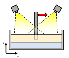
(a)

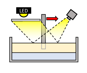
(b)

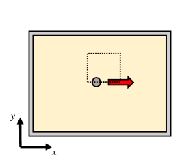
(c)

Figure 1: Schematic of the experimental set-up. (a) PIV set-up with two cameras, (b) texture set-up with the backlit acrylic plate and (c) birds-eye-view of the suspension surface with the dotted square indicating the investigation region of the present study. In the images, the beige layer represents the suspension and the blue layer beneath it represents a layer of Fluorinert.

The suspension is pre-sheared by towing the cylinder back and forth equivalent to an actual run, before any measurements are taken. When capturing particle images for the PIV, two 4 megapixel high-speed cameras (Photron FASTCAM Mini WX100) view the suspension surface in front and behind the traversing cylinders (figure 1(a)). Pulsed LED lighting was used to illuminate the surface and was synchronised with the camera acquisition at 750 Hz. The particle images were converted to velocity fields with LaVision DaVis 8.4.0 PIV software. An initial pass was performed with $96$ pixels $\times$ $96$ pixels square interrogation windows, followed by two passes with circular interrogation windows with decreasing size ending at $48$ pixels $\times$ $48$ pixels. For all passes, the interrogation windows have a $50$% overlap. The resulting instantaneous velocity fields are stitched together in post processing, masking out the cylinder in each frame. This results in a velocity field fully surrounding the cylinder.

As mentioned above, only minor adjustments to the set-up are needed in order to observe the surface features. This is illustrated in figure 1(b). Here, a single camera is positioned such that it views a direct reflection of a backlit, semi-transparent, acrylic sheet on the suspension surface. This enhances any surface features not captured by the PIV; note that the tracer particles used for PIV also interfere with the detection of the surface topology, which is why a separate campaign was used for surface texture measurements. Figure 1(c) gives a birds eye view of the suspension surface. For the scope of this work, we focus on the region indicated by the dotted square. See Rømcke et al (2021) for details on the full velocity field.

For the texture images, LaVision Davis 8.4.0 was used to find a third order calibration polynomial, mapping the image coordinates ($i,j$) to the lab coordinates ($x,y$). Matlab was used for all further processing of the texture images. Here, for consistency, the results are always plotted in the calibrated lab coordinate system ($x,y$). However, calculations on the surface features are done in pixel coordinates ($i,j$), and the results in ($i,j$) are mapped to ($x,y$) with the calibration polynomial.

Examples of both the PIV and texture images are shown in figure 2. The cylinder position is denoted $x_{c}$, which starts as $x=0$ and moves in the positive x-direction. The raw particle images (figures 2a-d) do not provide any information on the suspension texture. The resulting velocity fields from the PIV analysis of these images are shown in figures 2e-h. Note the sharp transition in velocity that propagates away from the cylinder as it moves through the flow. By the end of an experimental run, the whole field of view is moving with the cylinder as shown in figure 2h. The $0.5U_{c}$ contour is represented by the black line and used as a proxy for the position of the jamming front as is common in previous studies (Waitukaitis and Jaeger, 2012; Peters and Jaeger, 2014; Peters et al, 2016; Han et al, 2016, 2018, 2019b, 2019a; Rømcke et al, 2021).

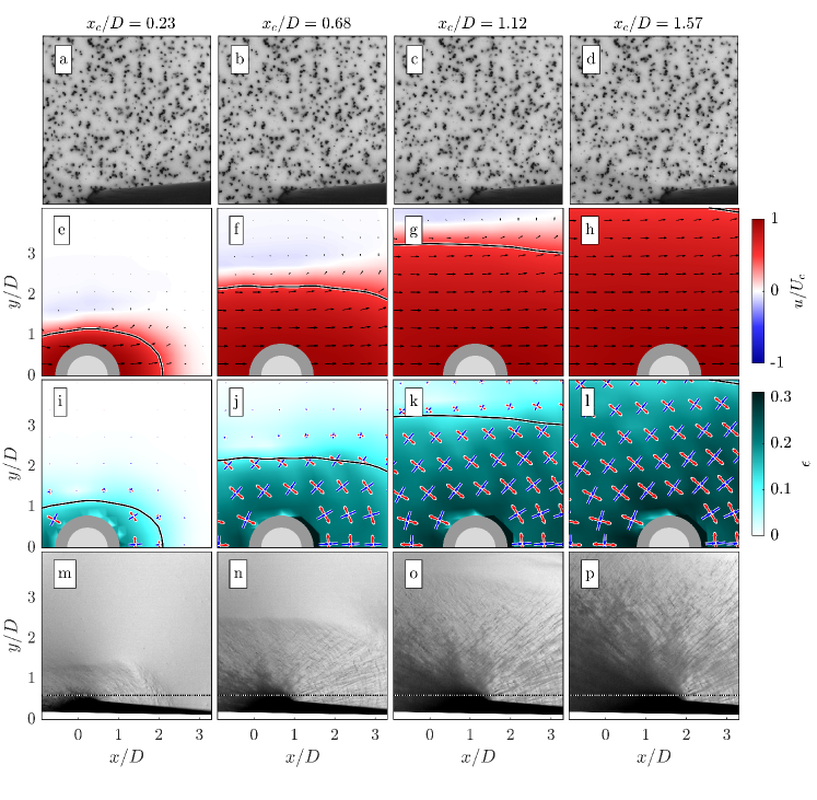
Figure 2: Time series comparison between PIV and texture images. $x_{c}$ represents the location of the cylinder. (a-d) Raw PIV particle images. (e-h) Resulting PIV velocity fields with superimposed velocity vectors. (i-l) Accumulated strain ($\epsilon$) with superimposed eigenvectors. Red represents the direction of stretch ($\mathbf{n}_{1}$), while blue indicates the direction of compression ($\mathbf{n}_{2}$). For clarity, $\mathbf{n_{i}}$ are scaled with $\epsilon$. In (e-l) the jamming front ($0.5U_{c}$ contour) is represented by the black line. (m-p) Surface features as the front propagates. In order to avoid the cylinder shadow, the analysis is restricted to the region above the dotted line.

From the velocity data, we estimate the local accumulated strain. The strain is shown to be an important parameter with regards to jamming. Given that the suspension is subjected to a sufficient amount of stress, an intrinsic onset strain dictates the amount of strain needed before the suspension transitions into a jammed state (Majumdar et al, 2017; Han et al, 2016, 2019a; Rømcke et al, 2021). The nominal value of the onset strain depends on the volume fraction (Han et al, 2016, 2018, 2019a). We define the strain in the same manner as Rømcke et al (2021). In short, by estimating the movement of the material points $\mathbf{x_{p}}(\mathbf{X},t)=\mathbf{X}+\int_{0}^{t}\mathbf{u}(\mathbf{x_{p}}(\tau),\tau)d\tau$, we calculate the deformation gradient tensor $\mathbf{F}=\frac{\partial\mathbf{x_{p}}}{\partial\mathbf{X}}$, where $\mathbf{X}$ is the position of the material points at $t=0$. From the deformation gradient the left stretch tensor $\mathbf{V}$ is acquired from a polar decomposition $\mathbf{F}=\mathbf{VR}$. The tensor $\mathbf{V}$ has eigenvalues and eigenvectors, $\lambda$ and $\mathbf{n}$, respectively. Here, we employ the Eulerian logarithmic strain tensor (Nemat-Nasser, 2004)

$$\mathbf{e}=\sum_{i}\ln(\lambda_{i})\mathbf{n}_{i}\otimes\mathbf{n}_{i}.$$ (2)

Eigenvalues are ordered $\lambda_{1}>\lambda_{2}$, such that $\mathbf{n}_{1}$ and $\mathbf{n}_{2}$ signify the direction of stretch and compression, respectively; $\mathbf{n}_{1}$ and $\mathbf{n}_{2}$ are orthogonal. Figures 2i-l show the evolution of the norm of the strain tensor $\epsilon=||\mathbf{e}||$. The strain ($\epsilon$) at the jamming front is relatively constant throughout an experiment (Rømcke et al, 2021), and measured to be $\sim 0.14$ in the case presented here. In the current work, we will focus on the orientation of the eigenvectors. Though the strain field is relatively homogeneous by the end of an experimental run (figure 2l), the superimposed eigenvectors show that the direction in which the suspension is stretched and compressed depends on the location in the flow.

Finally, a time series of the texture experiment is presented in figure 2m-p. Due to the specific lighting conditions explained above, this experiment reveals features not visible in the PIV particle images. Two key observations form the scope of this work. First, like the velocity field, there is a sharp transition between the regions with and without surface structures. This transition propagates from the cylinder, into the suspension, leaving a textured surface in its wake. We observe a change from a reflective to a matte surface indicative of a dilated suspension (Brown and Jaeger, 2012; Maharjan et al, 2021; Bischoff White et al, 2010; Smith et al, 2010). Second, by comparing the eigenvectors of the strain tensor (figure 2i-l) and the orientation of the surface features (figure 2m-p), there appears to be a connection. More specifically, the eigenvectors and surface features appear to be oriented in the same direction at the same locations in the flow, suggesting the raw surface images may hold quantifiable information akin to the PIV. This is explored further below.

3 Analysis methodology

The aim of this study is to quantify the structures observed at the free surface of a dense suspension undergoing dynamic jamming. In this section, we present a method that is able to identify surface features and their orientation. In short, images of the free surface are divided into interrogation windows, and the 2D fast Fourier transform (FFT) of the local windows is used as a basis for quantifying these structures, which is presented in section 3.1. Section 3.2 establishes a basis by which this process can be optimised and determines the optimal parameter values used in the remainder of this work.

3.1 FFT and sector averaging

Here, in order to extract local information from the texture images, such as how dominant the features are and what orientation they have, we divide the frame into interrogation windows. Figure 3 gives examples of four representative windows, which we will focus on in this section. As a first step towards quantifying the surface features, we take a 2D FFT of each window ($I(i,j)\xrightarrow{\mathcal{F}}\hat{I}(k_{i},k_{j})$); using an FFT to gain information on the surface texture is a common practice for interfacial flows, e.g., (Zhang, 1996; Loimer et al, 2002; Timberlake and Morris, 2005; Singh et al, 2006). The mean pixel intensity of the interrogation window is subtracted before calculating the FFT. Here, $I$ and $\hat{I}$ represent the intensity in the image and wave number domain, respectively.

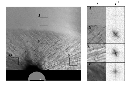
Figure 3: A snapshot of the suspension surface. Example interrogation windows are presented in the right columns with both the pixel intensity ($I$) and the 2D power spectra ($|\hat{I}|^{2}$). The intensity scale of the power spectra is plotted logarithmically. $200\times 200$ pixel interrogation windows representing (A) no features, (B and C) distinct features, (D) weak features.

The resulting FFTs of the interrogation windows are seen in the right column of figure 3 represented here by the power spectral density $|\hat{I}|^{2}$. Notice how the streaks in the interrogation windows are reflected in the corresponding power spectra. For B and C, the power spectra show clear features orthogonal to the streaks observed in the image. This trend is also observed for D, though clustered at lower wave numbers. Window A, however, has an almost perfectly homogeneous intensity, which is reflected in the power spectrum by predominantly exhibiting values at the noise level. An unwanted feature is also revealed by the FFT. As seen in the power spectra of A and D, a signal is observed along the lines $k_{i}=0$ and $k_{j}=0$. Though the background subtraction removes most of these features, they are still significant for low signal-to-noise ratio regions, e.g., A and D. For any further processing, this issue is addressed by masking out the values at the lines $k_{i}=0$ and $k_{j}=0$.

The general shape of the power spectra encodes both how dominant the features are and in what direction they are oriented. We extract the shape of a power spectrum by taking a sectional average. First, we denote the wave vector $\mathbf{k}=(k_{i},k_{j})$, so that in polar coordinates, $k=|\mathbf{k}|$ with the angle $\theta=\tan^{-1}(k_{j}/k_{i})$. The averaging procedure is taken over the wave number $k$ ranging from $0$ to $0.5$ pixel^-1 in sectors of size $\Delta\theta$. In polar coordinates, the average over a sector is represented by the integral

$$f(\theta,\Delta\theta)=\frac{8}{\Delta\theta}\int_{0}^{1/2}\int_{\theta-\Delta\theta/2}^{\theta+\Delta\theta/2}|\hat{I}|^{2}(k,\theta)k\,\text{d}\theta\,\text{d}k.$$ (3)

Numerically, given the discrete values of $|\hat{I}|^{2}$, the circle is divided into a number ($N$) of equally spaced angular sectors with a relative overlap $\xi$, shown schematically in figure 4(a). Note that $\Delta\theta=2\pi/(N(1-\xi))$. The sector average is calculated as the mean of $|\hat{I}|^{2}$ contained within the sector. Figures 4(b) and 4(c) show how the trend in the power spectra is reflected in the resulting curve $f$.

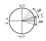
(a)

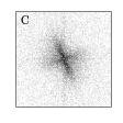
(b)

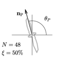
(c)

Figure 4: Schematics of the sector averaging. (a) Two neighbouring sectors with overlap. (b) Power spectra of interrogation window C with (c) resulting sector average curve ($f$) calculated with $N=48$ sectors and $\xi=50$% overlap. The vector $\mathbf{n}_{P}$ and the angle $\theta_{P}$ represent the orientation of the peak.

We use the sector average curve, $f$, to extract key features of a power spectrum. First, we calculate the shape factor, $S$, of the sector average curve in order to distinguish between an interrogation window with and without surface structure. $S$ is a measure of how much a shape resembles a circle. The shape factor is defined such that it compares the perimeter ($\delta$) of $f$ with the circumference of a circle with the same area ($\alpha$) as $f$, i.e.,

$$S=\frac{2\sqrt{\pi}\sqrt{\alpha}}{\delta}.$$ (4)

The shape factor $S$ is in the range $0$ to $1$, where $1$ represents a perfect circle. The power spectrum of window A from figure 3 is relatively uniform, and is expected to show values of $S$ close to unity. This can also be seen by substituting in a constant value for $|\hat{I}|^{2}$ in (4) resulting in $f(\theta)=$ constant. Window C, on the other hand, is expected to show values distinguishable from a perfect circle as we observe clear angular dependencies. Secondly, we take the orientation of the peak of $f$ to represent the orientation of the dominant surface features. In the image coordinates $(i,j)$, we denote the orientation of the peak $\theta_{P}^{*}$ which defines the unit vector $\mathbf{n}_{P}^{*}=(\cos{\theta_{P}^{*}},\ \sin{\theta_{P}^{*}})$. The unit vector is mapped to the spatial coordinate system with the calibration, such that $\mathbf{n}_{P}=(\cos(\theta_{P}),\ \sin(\theta_{P}))$, where $\theta_{P}$ represents the orientation of the peak in the $(x,y)$-system. Note that the Fourier transform is symmetric about the origin, thus two equal sized peaks separated by an angle $\pi$ are observed in figure 4(c). As a representation of the main direction of the structures, we only focus on peaks in the upper half plane $0\leq\theta_{P}<\pi$.

3.2 Determining processing parameters

Some parameters have been presented in the previous section that affect the sector average curve $f$. Here, we focus on the size of the interrogation window, as well as the number of sectors ($N$) and the sector overlap ($\xi$). Adjusting these parameters will consequently have an impact on $S$ and $\theta_{P}$. As one of our aims is to be able to distinguish between regions with surface features (such as window C) from regions without surface features (such as window A), we choose to use a set of processing parameters that will maximize the difference in $S$ between these two scenarios.

Trends of $S$ for window A and C over a range of processing parameters ($N$ and $\xi$) are presented in figure 5. As expected, the sector average curve, $f$, for window A (figure 5(a)) takes on a circular shape, while for window C (figure 5(b)), the curve indicates clear peaks orthogonal to the streaks on the surface. This is also reflected by the values of $S$ showing higher values for window A compared to C. However, in the extreme cases, the difference in $S$ tends to be small. For example, choosing a large number of sectors and a small overlap, even though the the resulting sector average curve from C shows clear peaks and a low shape factor, the shape factor of A is also reduced. On the other hand, choosing few sectors with a large overlap yields an almost perfect circular result for window A, but the peaks in C are no longer clear and the shape factor is higher. Figure 5 indicates that there is an optimal combination of $N$ and $\xi$ that would maximize the difference in shape factor $S$, such that the shape factor yields a clear distinction between the two scenarios.

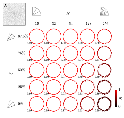
(a)

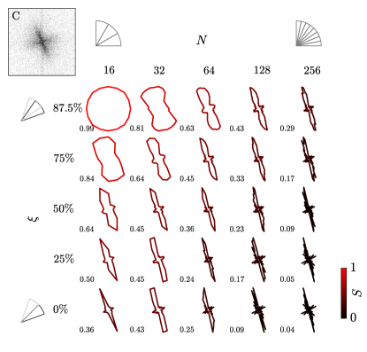
(b)

Figure 5: Sector average curves ($f$) for $256\times 256$ pixels interrogation windows of (a) A and (b) C over a range of overlap ($\xi$) and number of sectors ($N$). The resulting shape factor ($S$) is indicated by the color scheme and also presented numerically for each curve. For the remainder of this work, we choose $N=128$ and $\xi=75$ %.

We point out that the result presented in figure 5 only compares two locations in the flow (A and C) for one window size ($256\times 256$ pixels) from a specific snapshot of the flow. However, the trend is the same when comparing window A with window B and D over a range of window sizes from $64\times 64$ to $512\times 512$ pixels. After considering different window sizes and values for $N$ and $\xi$, the overall difference in $S$ appears to converge with increasing window size at $256\times 256$ pixels. Setting $N=128$ and $\xi=75$ % gives a sufficiently large difference in $S$, while simultaneously ensuring a satisfactory angular resolution for establishing $\theta_{P}$. For the remainder of this work, we will use a window size of $256\times 256$ pixels, with $N=128$ and $\xi=75$ % when computing the sector average curve, $f$. It would be important to note that the “optimal” is dependent on the specific experimental set-up and that the results found here would not be universally optimal akin to how PIV processing parameters are optimised individually for each experiment.

4 Results

The method outlined in section 3 is now applied to the full texture images. Section 4.1 presents results from the texture images alone. By setting a threshold value for $S$, we identify the textured region and in section 4.2 we give an estimate of how fast this region propagates into the suspension. In section 4.3, the data extracted from analysing the texture images are directly compared to the PIV data. First we present the combined evolution of the shape factor and velocity field. We then show that in certain regions of the flow, the direction of the texture and the eigenvectors of the strain tensor are predominantly oriented in the same direction.

4.1 Quantifying the texture for the full field

From the method presented above, we are capable of identifying if the surface shows features ($S$), and in what direction the features are oriented ($\mathbf{n}_{P}$). Both $S$ and $\mathbf{n}_{P}$, are presented in figure 6. The analysis is conducted on the full field of the time series shown in figure 2m-p, with the processing parameters found in section 3.2. In addition, we let neighbouring interrogation windows overlap with $75$%.

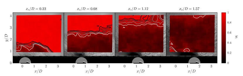
(a)

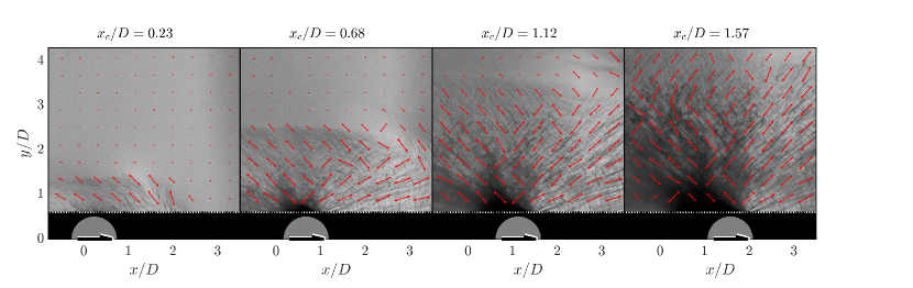
(b)

Figure 6: Texture analysis on the full field of the snapshots in figure 2m-p. (a) Shape factor $S$. The contours represent $S=0.6$, $0.7$, $0.8$ $0.85$ and $0.9$, where the $0.85$ is represented by the dotted line. (b) Orientation of the peak ($\mathbf{n}_{P}$) from the sector average, which is represented by the vectors superimposed on the corresponding surface image. Every third vector is plotted to reduce clutter, and scaled with $1-S$. In addition, $\mathbf{n}_{P}$ is rotated by $\pi/2$ such that the vectors point in the same direction as the surface streaks rather than normal to them.

Figure 6(a) shows that the shape factor clearly separates the flow into two regions. Five iso-contours, $S=0.6$, $0.7$, $0.8$, $0.85$ and $S=0.9$, are superimposed on the $S$-field. Here, these contours tend to cluster at the transition between the textured and texture-free surface. Analogous to the $0.5U_{c}$ contour being used to identify the position of the jamming front from PIV data, a contour level between $S=0.6$ and $S=0.9$ identifies the position of the front from the texture data. In the later stages of an experimental run, dilation renders the surface matte. Due to the increase in $S$ observed in figure 6(a), it becomes increasingly difficult to identify the preferred texture orientation in some parts of the flow. This is most noticeable in the wake of the cylinder.

The corresponding orientation of the surface features are indicated in figure 6(b). As noted in figures 4 and 5, the peak in $f$ is oriented normal to the direction of the dominant streaks in the texture image. For clarity in figure 6(b), the vectors indicating the peak angle, $\mathbf{n}_{P}$, are rotated by $\pi/2$ such that they are oriented parallel to the surface streaks. Here, we plot both $\mathbf{n}_{P}$ and $-\mathbf{n}_{P}$, representing the symmetry of the power spectra.

The orientation of the vectors can be directly compared to the actual texture image. Notice that fore (aft) of the cylinder, the vectors generally tend to be forward (backward) leaning, reflecting the dominant streaks in the region. The region roughly around the same $x$-location as the cylinder, exhibits a crosshatch pattern (Chang et al, 1990; Albrecht et al, 1995). This is more clearly indicated in figure 3 by window B. As we only report the most dominant peak in $f$, the vectors $\mathbf{n}_{P}$ generally show a mix of forward-leaning and backward-leaning in this region. Notice the similarity with the eigenvectors plotted in figures 2i-l; $\mathbf{n}_{1}$, representing direction of stretch, is backwards-leaning, while $\mathbf{n}_{2}$, representing compression, forward leaning. The similarity between $\mathbf{n}_{P}$ and the strain eigenvectors will be addressed in greater detail in section 4.3.

4.2 Propagation of the texture transition

Figure 7 establishes the location of the texture transition, and estimates its propagation velocity into the suspension. Here, we focus on the transverse direction relative to the cylinder velocity. As with the jamming front position being identified by the $0.5U_{c}$ contour, we will identify the texture transition by a contour value in $S$. We will compare how fast the jamming front and texture transition propagates into the suspension.

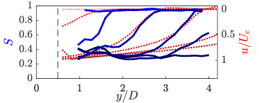
(a)

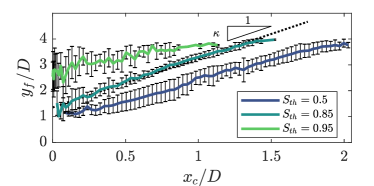
(b)

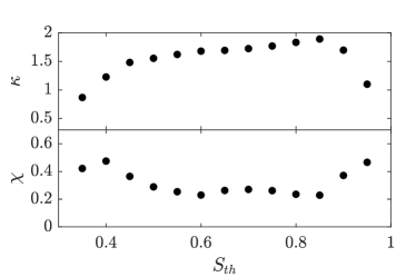
(c)

Figure 7: (a) Profiles of the shape factor (solid blue lines) and velocity (dotted red lines) for an experimental run in vertical cross sections taken at the location of the cylinder ($x=x_{c}$). The black dashed line indicates the location of the cylinder surface. The color intensity indicates different $x_{c}$ as the cylinder moves through the flow. Velocity profiles are flipped to emphasize the similarity between $S$ and $u$ (b) Position of the front, $y_{f}$, for three different threshold values of the shape factor. The slope of the linear regression line is denoted $\kappa$. (c) Slope, $\kappa$, and RMS of the error of the regression line, $\chi$, as functions of the threshold value, $S_{th}$.

The front propagation factor, denoted here by $\kappa$, is defined as the relation between the speed of the jamming front and the speed of the perturbing body. In the transverse direction relative to the cylinder velocity, the front propagation factor is the time derivative of the jamming front’s $y$-position ($y_{f}$) relative to the speed of the cylinder ($U_{c}$). Since

$$\kappa=\frac{dy_{f}/dt}{U_{c}}\approx\frac{\Delta y_{f}/\Delta t}{\Delta x_{c}/\Delta t}=\frac{\Delta y_{f}}{\Delta x_{c}},$$ (5)

rather than estimating a time derivative, we will focus on the equivalent relation $\Delta y_{f}/\Delta x_{c}$. As such, for the texture data, we start by establishing the position of the texture transition.

As seen by the superimposed contours in figure 6(a), the position of the texture transition depends on the choice of contour level. Figure 7(a) shows vertical cross sections of the shape factor taken as the cylinder translate in the $x$-direction ($S(x=x_{c},y)$, where $x_{c}$ represents the instantaneous cylinder position). As with the velocity profiles (indicated by the dotted lines in figure 7(a)), $S$ is not a perfect step, and as pointed out above, the position of the front will depend on the choice of the contour level. We use $y_{f}$ to denote the position of the texture transition and is given implicitly from the shape factor profiles as $S_{th}=S(x=x_{c},y_{f})$. Here, $S_{th}$ represents the contour level, or the threshold value for $S$ separating textured from texture free surface. Numerically, the front position is acquired by linearly interpolating the shape factor profiles, e.g. figure 7(a).

The resulting front position ($y_{f}$) from all experimental runs is plotted in figure 7(b) for three different values of $S_{th}$. Due to variation in the front position shown in figure 7(b), calculating the relation $\Delta y_{f}/\Delta x_{c}$ directly has large uncertainties associated with it. Instead, we report the slope of the linear regression line through the data, with the root mean square of the error denoted as $\chi$. Figure 7(c) shows $\kappa$ and $\chi$ as functions of $S_{th}$. The error tends to show a minimum in the range $0.5<S_{th}<0.9$ with values $\chi\approx 0.2$. Note that this range of shape factor values are generally where we see the sharpest gradients in the $S$-profiles plotted in figure 7(a) and also indicated by the superimposed contours in figure 6(a).

The minimum error is found at $S_{th}=0.85$ where the slope is $\kappa=1.89$. From the velocity field, we measure a front propagation factor in the transverse direction as $\kappa_{PIV}=1.96\pm 0.4$. It should be noted that the speed estimated from the PIV is from the $0.5U_{c}$ contour, which is itself a surrogate, albeit a commonly used one (Waitukaitis and Jaeger, 2012; Peters and Jaeger, 2014; Han et al, 2016; Peters et al, 2016; Majumdar et al, 2017; Han et al, 2018, 2019b; Baumgarten and Kamrin, 2019; Rømcke et al, 2021). Thus, our method shows that the propagation of the texture transition, and the propagation of the jamming front are comparable.

4.3 Comparing texture and PIV data for the full field

Similarities between the texture measurements and the PIV data have been noted in the previous sections. Here, we address the full field of view explicitly. Most notably, the evolution of the region exhibiting surface features (that is $S<0.85$ in figure 6(a)) and the region traversing with the cylinder (that is $u/U_{c}>0.5$ in figure 2e-h). In addition, it is observed that the surface features (figure 6(b)) and the eigenvectors of the strain tensor ($\mathbf{n}_{1}$ and $\mathbf{n}_{2}$ in figure 2i-l) are approximately oriented in the same directions. This section aims to quantify these observations.

The combined evolution of the shape factor and velocity are plotted in figure 8. As indicated in figure 2 and 6(a), the overall trend of the data is to transition from a state of low velocity ($u/U_{c}<0.5$) and high shape factor ($S>0.85$) to a state of high velocity ($u/U_{c}>0.5$) and low shape factor ($S<0.85$). In other words, the suspension transitions from a quiescent suspension with no notable surface features, to moving with the cylinder while exhibiting observable surface features. Importantly, figure 8 shows that the transition between these two states occurs at the same time in the experiment.

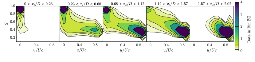
Figure 8: Evolution of the velocity, $u$, from the PIV experiment and shape factor, $S$, from the texture experiment. The figures are 2D histograms indicating where the data points tend to cluster for different stages in the experiment.

In addition, we seek to rigorously confirm that the surface features and eigenvectors are oriented in the same direction. This analysis is only relevant where the suspension has deformed sufficiently and the surface exhibit clear surface features. As such, the data will be separated into regions where the analysis is conducted separately.

As a first step towards identifying the relevant region, figure 9(a) shows the histogram of $S$ and $u/U_{c}$ similar to figure 8 for the full time series and all experimental runs. By using the threshold value $S_{th}=0.85$ for the shape factor (see section 4.2) and the definition of the jamming front ($u/U_{c}=0.5$), we divide the data into quadrants. Here, $Q1$ represents a slow moving texture free state, $Q2$ represents the transition, while $Q3$ represents the suspension moving with the cylinder exhibiting measurable surface features. It is worth noting that $Q1$, $Q2$ and $Q3$ contain roughly $35$, $15$ and $50$ % of the data, respectively. The unlabeled quadrant in figure 9(a) contains less than $1$ % of the data, and its contribution is negligible. An example of where these regions are located in the flow is presented in figure 9(b). This figure compares the velocity field in figure 2f with the result of the shape factor $S$ acquired from figure 2n.

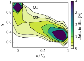
(a)

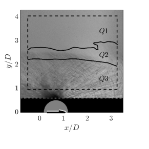
(b)

Figure 9: (a) Histogram of $S$ and $u/U_{c}$ similar to figure 8 for the whole time series for all experimental runs. The dashed lines separates the data into quadrants $Q1$, $Q2$ and $Q3$. (b) Example of how the quadrants represent different regions of the system. This particular snapshot compares the velocity field and texture from figure 2f and 2n.

A representation of the texture orientation and the strain eigenvectors are presented in figure 10(a). The orientations are arbitrary, and the figure is only meant to be illustrative. The vectors are normalized to unit vectors. $\mathbf{n}_{P}$ is defined in section 3.1 and represents the orientation of the texture. As a basis for comparing texture and eigenvector orientation we will use the dot products $\mathbf{n}_{1}\cdot\mathbf{n}_{P}$ and $\mathbf{n}_{2}\cdot\mathbf{n}_{P}$. Since all three vectors are unit vectors, these dot products represents the cosine of the angle separating them.

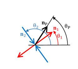
(a)

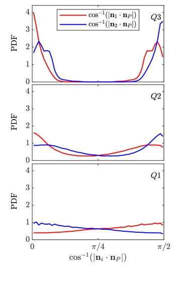
(b)

Figure 10: (a) Schematic representation of texture orientation, $\mathbf{n}_{P}$, and strain eigenvectors where $\mathbf{n}_{1}$ represents stretch and $\mathbf{n}_{2}$ represents compression. (b) PDFs of the angle separating $\mathbf{n}_{P}$ and $\mathbf{n}_{i}$ for the regions $Q1$, $Q2$ and $Q3$, respectively.

Figure 10(b) shows probability density functions (PDF) of $\cos^{-1}(|\mathbf{n}_{i}\cdot\mathbf{n}_{P}|)$ for the regions $Q1$, $Q2$ and $Q3$, respectively. The absolute value of the dot product is used here, thus representing the angle separating $\mathbf{n}_{P}$ and the span of the eigenvectors $\mathbf{n}_{i}$ with a positive value. As a result, $\cos^{-1}(|\mathbf{n}_{i}\cdot\mathbf{n}_{P}|)=0$ indicates $\mathbf{n}_{P}\parallel\mathbf{n}_{i}$, while $\cos^{-1}(|\mathbf{n}_{i}\cdot\mathbf{n}_{P}|)=\pi/2$ indicates $\mathbf{n}_{P}\perp\mathbf{n}_{i}$. As seen in figure 10(b), the texture vectors are somewhat biased towards $\mathbf{n}_{2}$ in the $Q1$ region. In the transition region, $Q2$, the texture $\mathbf{n}_{P}$ starts to favor the $\parallel$ and $\perp$ directions relative to the strain. For $Q3$, the PDFs are $\approx 0$ in the region $\pi/8<\cos^{-1}(|\mathbf{n}_{i}\cdot\mathbf{n}_{P}|)<3\pi/8$ with strong peaks at $0$ and $\pi/2$. In other words, the PDFs from region $Q3$ clearly show that the texture observed at the free surface has a strong connection with the orientation of the eigenvectors of the strain tensor.

5 Conclusion

Measurements of how surface texture evolves on a dense suspension of cornstarch and water with a freely propagating shear jamming front have been presented. The surface texture is captured by high-speed images of the free surface looking into a direct reflection. PIV measurements are used as a reference. From images of the surface texture, a 2D fast Fourier transform of local interrogation windows is used as a basis for analysing the surface structure. By taking a sector average of the power spectra, we are able to identify whether surface features are observed and the direction they are oriented.

The PIV and texture measurements are two separate experiments, however, we show that the region of the suspension that shows clear surface features overlaps with the jammed region. In addition, we show that in the jammed, textured region of the flow, the eigenvectors of the strain tensor, and the observed surface features are oriented in the same direction. Hence, our analysis reveals that pictures of the free surface contain quantifiable information not previously directly accessed.

Dilation (Brown and Jaeger, 2012; Jerome et al, 2016; Majumdar et al, 2017; Maharjan et al, 2021) as well as surface corrugations (Loimer et al, 2002; Timberlake and Morris, 2005) have been observed at the free surface of dense suspensions before. However, few studies have investigated the surface texture at a freely propagating shear jamming front (Allen et al, 2018). The results presented in the current work, particularly the relation between the eigenvectors of the strain tensor and the orientation of the surface features, will provide insight for future model development and understanding of dense suspensions as well as a valuable measurement tool for future investigations.

References

- Albrecht et al (1995) Albrecht M, Christiansen S, Michler J, Dorsch W, Strunk HP, Hansson PO, Bauser E (1995) Surface ripples, crosshatch pattern, and dislocation formation: Cooperating mechanisms in lattice mismatch relaxation. Applied Physics Letters 67(9):1232–1234, DOI 10.1063/1.115017, URL https://doi.org/10.1063/1.115017, https://doi.org/10.1063/1.115017
- Allen et al (2018) Allen B, Sokol B, Mukhopadhyay S, Maharjan R, Brown E (2018) System-spanning dynamically jammed region in response to impact of cornstarch and water suspensions. Phys Rev E 97:052,603, DOI 10.1103/PhysRevE.97.052603, URL https://link.aps.org/doi/10.1103/PhysRevE.97.052603
- Baumgarten and Kamrin (2019) Baumgarten AS, Kamrin K (2019) A general constitutive model for dense, fine-particle suspensions validated in many geometries. Proceedings of the National Academy of Sciences 116(42):20,828–20,836, DOI 10.1073/pnas.1908065116, URL https://www.pnas.org/content/116/42/20828, https://www.pnas.org/content/116/42/20828.full.pdf
- Bischoff White et al (2010) Bischoff White EE, Chellamuthu M, Rothstein JP (2010) Extensional rheology of a shear-thickening cornstarch and water suspension. Rheologica acta 49(2):119–129
- Brown and Jaeger (2012) Brown E, Jaeger HM (2012) The role of dilation and confining stresses in shear thickening of dense suspensions. Journal of Rheology 56(4):875–923, DOI 10.1122/1.4709423, URL https://doi.org/10.1122/1.4709423, https://doi.org/10.1122/1.4709423
- Brown and Jaeger (2014) Brown E, Jaeger HM (2014) Shear thickening in concentrated suspensions: phenomenology, mechanisms and relations to jamming. Reports on Progress in Physics 77(4):046,602
- Cates and Wyart (2014) Cates ME, Wyart M (2014) Granulation and bistability in non-brownian suspensions. Rheologica acta 53(10):755–764
- Cates et al (2005) Cates ME, Haw MD, Holmes CB (2005) Dilatancy, jamming, and the physics of granulation. Journal of Physics: Condensed Matter 17(24):S2517–S2531, DOI 10.1088/0953-8984/17/24/010, URL https://doi.org/10.1088/0953-8984/17/24/010
- Chang et al (1990) Chang KH, Gilbala R, Srolovitz DJ, Bhattacharya PK, Mansfield JF (1990) Crosshatched surface morphology in strained iii‐v semiconductor films. Journal of Applied Physics 67(9):4093–4098, DOI 10.1063/1.344968, URL https://doi.org/10.1063/1.344968, https://doi.org/10.1063/1.344968
- Denn et al (2018) Denn MM, Morris JF, Bonn D (2018) Shear thickening in concentrated suspensions of smooth spheres in Newtonian suspending fluids. Soft Matter 14:170–184, DOI 10.1039/C7SM00761B, URL http://dx.doi.org/10.1039/C7SM00761B
- Fernandez et al (2013) Fernandez N, Mani R, Rinaldi D, Kadau D, Mosquet M, Lombois-Burger H, Cayer-Barrioz J, Herrmann HJ, Spencer ND, Isa L (2013) Microscopic mechanism for shear thickening of non-Brownian suspensions. Phys Rev Lett 111:108,301, DOI 10.1103/PhysRevLett.111.108301, URL https://link.aps.org/doi/10.1103/PhysRevLett.111.108301
- Gadala‐Maria and Acrivos (1980) Gadala‐Maria F, Acrivos A (1980) Shear‐induced structure in a concentrated suspension of solid spheres. Journal of Rheology 24(6):799–814, DOI 10.1122/1.549584, URL https://doi.org/10.1122/1.549584, https://doi.org/10.1122/1.549584
- Guazzelli and Pouliquen (2018) Guazzelli E, Pouliquen O (2018) Rheology of dense granular suspensions. Journal of Fluid Mechanics 852:P1, DOI 10.1017/jfm.2018.548
- Guy et al (2015) Guy BM, Hermes M, Poon WCK (2015) Towards a unified description of the rheology of hard-particle suspensions. Phys Rev Lett 115:088,304, DOI 10.1103/PhysRevLett.115.088304, URL https://link.aps.org/doi/10.1103/PhysRevLett.115.088304
- Han et al (2016) Han E, Peters IR, Jaeger HM (2016) High-speed ultrasound imaging in dense suspensions reveals impact-activated solidification due to dynamic shear jamming. Nature Communications 7(1), DOI 10.1038/ncomms12243
- Han et al (2018) Han E, Wyart M, Peters IR, Jaeger HM (2018) Shear fronts in shear-thickening suspensions. Phys Rev Fluids 3:073,301, DOI 10.1103/PhysRevFluids.3.073301, URL https://link.aps.org/doi/10.1103/PhysRevFluids.3.073301
- Han et al (2019a) Han E, James NM, Jaeger HM (2019a) Stress controlled rheology of dense suspensions using transient flows. Phys Rev Lett 123:248,002, DOI 10.1103/PhysRevLett.123.248002, URL https://link.aps.org/doi/10.1103/PhysRevLett.123.248002
- Han et al (2019b) Han E, Zhao L, Van Ha N, Hsieh ST, Szyld DB, Jaeger HM (2019b) Dynamic jamming of dense suspensions under tilted impact. Phys Rev Fluids 4:063,304, DOI 10.1103/PhysRevFluids.4.063304, URL https://link.aps.org/doi/10.1103/PhysRevFluids.4.063304
- James et al (2018) James NM, Han E, Cruz RAL, Jureller J, Jaeger HM (2018) Interparticle hydrogen bonding can elicit shear jamming in dense suspensions. Nature Materials 17, DOI 10.1038/s41563-018-0175-5, URL https://doi.org/10.1038/s41563-018-0175-5
- Jerome et al (2016) Jerome JJS, Vandenberghe N, Forterre Y (2016) Unifying impacts in granular matter from quicksand to cornstarch. Phys Rev Lett 117:098,003, DOI 10.1103/PhysRevLett.117.098003, URL https://link.aps.org/doi/10.1103/PhysRevLett.117.098003
- Krieger (1972) Krieger IM (1972) Rheology of monodisperse latices. Advances in Colloid and Interface Science 3(2):111–136, DOI https://doi.org/10.1016/0001-8686(72)80001-0, URL https://www.sciencedirect.com/science/article/pii/0001868672800010
- Kumar et al (2016) Kumar AA, Medhi BJ, Singh A (2016) Experimental investigation of interface deformation in free surface flow of concentrated suspensions. Physics of Fluids 28(11):113,302, DOI 10.1063/1.4967739, URL https://doi.org/10.1063/1.4967739, https://doi.org/10.1063/1.4967739
- Lin et al (2015) Lin NYC, Guy BM, Hermes M, Ness C, Sun J, Poon WCK, Cohen I (2015) Hydrodynamic and contact contributions to continuous shear thickening in colloidal suspensions. Phys Rev Lett 115:228,304, DOI 10.1103/PhysRevLett.115.228304, URL https://link.aps.org/doi/10.1103/PhysRevLett.115.228304
- Loimer et al (2002) Loimer T, Nir A, Semiat R (2002) Shear-induced corrugation of free interfaces in concentrated suspensions. Journal of Non-Newtonian Fluid Mechanics 102(2):115–134, DOI https://doi.org/10.1016/S0377-0257(01)00173-2, URL https://www.sciencedirect.com/science/article/pii/S0377025701001732, a Collection of Papers Dedicated to Professor ANDREAS ACRIVOS on the Occasion of his Retirement from the Benjamin Levich Institute for Physiochemical Hydrodynamics and the City College of the CUNY
- Madraki et al (2017) Madraki Y, Hormozi S, Ovarlez G, Guazzelli E, Pouliquen O (2017) Enhancing shear thickening. Phys Rev Fluids 2:033,301, DOI 10.1103/PhysRevFluids.2.033301, URL https://link.aps.org/doi/10.1103/PhysRevFluids.2.033301
- Maharjan et al (2021) Maharjan R, O’Reilly E, Postiglione T, Klimenko N, Brown E (2021) Relation between dilation and stress fluctuations in discontinuous shear thickening suspensions. Phys Rev E 103:012,603, DOI 10.1103/PhysRevE.103.012603, URL https://link.aps.org/doi/10.1103/PhysRevE.103.012603
- Majumdar et al (2017) Majumdar S, Peters IR, Han E, Jaeger HM (2017) Dynamic shear jamming in dense granular suspensions under extension. Phys Rev E 95:012,603, DOI 10.1103/PhysRevE.95.012603, URL https://link.aps.org/doi/10.1103/PhysRevE.95.012603
- Mari et al (2014) Mari R, Seto R, Morris JF, Denn MM (2014) Shear thickening, frictionless and frictional rheologies in non-Brownian suspensions. Journal of Rheology 58(6):1693–1724, DOI 10.1122/1.4890747, URL https://doi.org/10.1122/1.4890747, https://doi.org/10.1122/1.4890747
- Mukhopadhyay et al (2018) Mukhopadhyay S, Allen B, Brown E (2018) Testing constitutive relations by running and walking on cornstarch and water suspensions. Phys Rev E 97:052,604, DOI 10.1103/PhysRevE.97.052604, URL https://link.aps.org/doi/10.1103/PhysRevE.97.052604
- Nemat-Nasser (2004) Nemat-Nasser S (2004) Plasticity : a treatise on finite deformation of heterogeneous inelastic materials. Cambridge monographs on mechanics, Cambridge University Press, Cambridge
- Peters and Jaeger (2014) Peters IR, Jaeger HM (2014) Quasi-2d dynamic jamming in cornstarch suspensions: visualization and force measurements. Soft Matter 10:6564–6570, DOI 10.1039/C4SM00864B, URL http://dx.doi.org/10.1039/C4SM00864B
- Peters et al (2016) Peters IR, Majumdar S, Jaeger HM (2016) Direct observation of dynamic shear jamming in dense suspensions. Nature 532(7598):214–217, URL http://search.proquest.com/docview/1781536995/
- Rømcke et al (2021) Rømcke O, Peters IR, Hearst RJ (2021) Getting jammed in all directions: Dynamic shear jamming around a cylinder towed through a dense suspension. Phys Rev Fluids 6:063,301, DOI 10.1103/PhysRevFluids.6.063301, URL https://link.aps.org/doi/10.1103/PhysRevFluids.6.063301
- Singh et al (2006) Singh A, Nir A, Semiat R (2006) Free-surface flow of concentrated suspensions. International Journal of Multiphase Flow 32(7):775–790, DOI https://doi.org/10.1016/j.ijmultiphaseflow.2006.02.018, URL https://www.sciencedirect.com/science/article/pii/S0301932206000486
- Singh et al (2018) Singh A, Mari R, Denn MM, Morris JF (2018) A constitutive model for simple shear of dense frictional suspensions. Journal of Rheology 62(2):457–468, DOI 10.1122/1.4999237, URL https://doi.org/10.1122/1.4999237, https://doi.org/10.1122/1.4999237
- Sivadasan et al (2019) Sivadasan V, Lorenz E, Hoekstra AG, Bonn D (2019) Shear thickening of dense suspensions: The role of friction. Physics of Fluids 31(10):103,103, DOI 10.1063/1.5121536, URL https://doi.org/10.1063/1.5121536
- Smith et al (2010) Smith M, Besseling R, Cates M, Bertola V (2010) Dilatancy in the flow and fracture of stretched colloidal suspensions. Nature Communications 114, DOI 10.1038/ncomms1119, URL https://doi.org/10.1038/ncomms1119
- Stickel and Powell (2005) Stickel JJ, Powell RL (2005) Fluid mechanics and rheology of dense suspensions. Annual Review of Fluid Mechanics 37(1):129–149, DOI 10.1146/annurev.fluid.36.050802.122132, URL https://doi.org/10.1146/annurev.fluid.36.050802.122132, https://doi.org/10.1146/annurev.fluid.36.050802.122132
- Tapia et al (2019) Tapia F, Pouliquen O, Guazzelli E (2019) Influence of surface roughness on the rheology of immersed and dry frictional spheres. Phys Rev Fluids 4:104,302, DOI 10.1103/PhysRevFluids.4.104302, URL https://link.aps.org/doi/10.1103/PhysRevFluids.4.104302
- Timberlake and Morris (2005) Timberlake BD, Morris JF (2005) Particle migration and free-surface topography in inclined plane flow of a suspension. Journal of Fluid Mechanics 538:309–341, DOI 10.1017/S0022112005005471
- Waitukaitis and Jaeger (2012) Waitukaitis SR, Jaeger HM (2012) Impact-activated solidification of dense suspensions via dynamic jamming fronts. Nature 487(7406):205, DOI 10.1038/nature11187
- Wyart and Cates (2014) Wyart M, Cates ME (2014) Discontinuous shear thickening without inertia in dense non-Brownian suspensions. Phys Rev Lett 112:098,302, DOI 10.1103/PhysRevLett.112.098302, URL https://link.aps.org/doi/10.1103/PhysRevLett.112.098302
- Zhang (1996) Zhang X (1996) An algorithm for calculating water surface elevations from surface gradient image data. Experiments in fluids 21(1):43–48