Higher order finite volume quantization conditions for two spinless particles

Abstract

Lattice QCD calculations of scattering phase shifts and resonance parameters in the two-body sector are becoming precision studies. Early calculations employed Lüscher’s formula for extracting these quantities at lowest order. As the calculations become more ambitious, higher-order relations are required. In this study we derive higher-order quantization conditions and introduce a method to transparently cross-check our results. This is an important step given the involved derivations of these formulas. We derive quantization conditions up to $\ell=5$ partial waves in both cubic and elongated geometries, and for states with zero and nonzero total momentum. All 45 quantization conditions we include here (22 in cubic box, 23 in elongated box) pass our cross-check test.

I Introduction

Hadron structure and interactions are controlled by the quark and gluon dynamics as described by quantum chromodynamics (QCD). Inside the hadrons the quarks and gluons interact strongly and nonperturbative methods are required to describe the interactions. Lattice QCD is used to study this dynamics in the Euclidean time framework. In this framework QCD spectrum for one or multiparticle states can be accessed directly. On the other hand, information about hadron interactions, in particular scattering properties, are accessed indirectly by calculating the energy of two-hadron states in finite volume. An intuition about this connection comes from understanding that the finite-volume energy shift for these states compared to the infinite volume setup is due to the interactions between the particles which in finite volume have a nonvanishing probability of being separated by distances comparable to the interaction range. The full details for this relation were worked out by Lüscher Lüscher (1991): he showed that the energy shifts for two-particle states in finite volume (with periodic boundary conditions) are directly controlled by the scattering phase shifts and the relations are model independent. These relations are exact, up to exponentially small finite-volume corrections, as long as the energy of the two particle states is below the inelastic threshold.

In the field of nuclear and particle physics, the method has proven especially successful. Various extensions to the method have since been made to enhance its applicability, including moving frames Rummukainen and Gottlieb (1995); Kim et al. (2005); Fu (2012); Leskovec and Prelovsek (2012); Gockeler et al. (2012); Li et al. (2021); Doring et al. (2012), asymmetric boxes Feng et al. (2004); Lee and Alexandru (2017); Li et al. (2021), multiple partial waves and coupled channel scattering LIU et al. (2006); Lage et al. (2009); Bernard et al. (2008); Döring et al. (2011); Hansen and Sharpe (2012); Luu and Savage (2011); Li and Liu (2013); Briceno and Davoudi (2013); Briceno (2014); Morningstar et al. (2017); Li et al. (2020). The use of asymmetric lattices has proven to be computationally efficient Pelissier and Alexandru (2013); Guo et al. (2016, 2018); Culver et al. (2019); Li et al. (2021) so we will include it in our discussions. The method has been widely applied to a multitude of meson-meson scattering processes, along with some meson-baryon and baryon-baryon systems over the past decade Pelissier and Alexandru (2013); Guo et al. (2016, 2018); Culver et al. (2019); Mai et al. (2019); Bulava et al. (2016); Brett et al. (2018); Andersen et al. (2019); Alexandrou et al. (2017); Bali et al. (2016); Feng et al. (2015, 2011); Orginos et al. (2015); Beane et al. (2012); Aoki et al. (2011); Dudek et al. (2013a, 2012a); Mohler et al. (2013a); Prelovsek et al. (2013); Mohler et al. (2013b); Lang et al. (2012, 2011); Guo et al. (2016); Helmes et al. (2017); Liu et al. (2017); Helmes et al. (2015); Wilson et al. (2015a, b); Moir et al. (2016). Significant progress towards a complete three-body scattering quantization condition has also been made in recent years, though we do not discuss it here. See Refs. Mai et al. (2021a, b); Fischer et al. (2021); Hansen and Sharpe (2019); Rusetsky (2019); Culver et al. (2020); Blanton et al. (2020); Alexandru et al. (2020); Brett et al. (2021); Hansen et al. (2021); Blanton et al. (2021) for reviews of theoretical developments, and some first applications to three-pion and kaon scattering.

The quantization conditions (QCs), that is the equations connecting the phase shifts to finite volume spectrum, are rather complex. Early lattice QCD scattering studies have employed only the lowest-order quantization conditions, which can be used to directly extract the phase shifts from finite-volume energies. As these calculations become more ambitious higher-order conditions, where several partial waves are involved, are required Dudek et al. (2012b, 2013b); Wilson et al. (2015c); Morningstar et al. (2017). Lüscher worked out these formulas for zero-momentum states of two equal-mass, spinless particles in a cubic box. Further work extended these relations for different kinematics Rummukainen and Gottlieb (1995); Fu (2012); Leskovec and Prelovsek (2012); Gockeler et al. (2012); Feng et al. (2004); Lee and Alexandru (2017); Morningstar et al. (2017); Luu and Savage (2011); Li and Liu (2013); Briceno and Davoudi (2013); Briceno (2014). These relations need to take into account the geometry of the box, the mass and spin of the hadrons, scattering channels, etc. In this work we compute the quantization conditions for two spinless particles in different kinematic situation for partial waves as high as $\ell=5$.

We note that the derivation of these formulas is fairly involved and the quantization conditions are expressed in terms of special functions that are nontrivial to calculate. Furthermore the coefficients appearing in these formulas depend on the symmetry group and the relevant irreducible representation. Some of the lower-order quantization conditions have been checked thoroughly, but the ones we derive in this work, for special cases and higher order, need to be cross-checked before they are used to extract scattering information from noisy lattice QCD data. To this end, we propose a method to check our derivations that is relatively transparent, especially for lattice QCD practitioners, and we use it to test our results with high accuracy in all possible channels for two spinless particles.

The paper is organized as follows. In Sec. II we review how the QC are derived and how they are connected to the irreducible representations of the symmetry group. We also discuss moving frames in nonrelativistic kinematics, and derive all the QCs we will investigate in this work. Then in Sec. III we discuss the method we used to check our results, that is our approach to computing the two-particle spectrum in a finite-volume box by solving the associated Schrödinger equation. The role of symmetries and their influence of the spectrum is first discussed here. In Sec. IV, we detail our numerical checks and compare the QC results with the spectrum derived in Sec. III. Some examples will be given. The rest will be available as Supplemental Material sup . In Sec. V, we summarize our findings and give future outlook. All group theory details are collected in Appendix A and all matrix elements in Appendix B.

II Quantization condition

Scattering is omnipresent in understanding the nature of interactions between particles. In infinite volume, nonrelativistic two-particle scattering can be captured by solving the Schrödinger equation in the center of mass (CM) frame,

$$\left[-\frac{\hbar^{2}}{2\tilde{m}}\nabla^{2}+V(r)\right]\psi(\bm{r})=E\psi(\bm{r}),$$ (1)

where $\tilde{m}=m_{1}m_{2}/(m_{1}+m_{2})$ is the reduced mass of the system. Elastic scattering phase shift is defined as the change in phase in the scattered wave relative to the incident wave in the asymptotic region where the interaction can be neglected. In the partial-wave expansion, the wave function satisfies the asymptotic condition,

$$\psi(\bm{r})=e^{ikz}+f(\theta)\frac{e^{ikr}}{r}$$ (2)

where $k$ is the relative CM momentum related to the energy $E=\hbar^{2}k^{2}/(2\tilde{m})$ and

$$f(\theta)=\sum_{l=0}^{\infty}(2l+1)f_{l}P_{l}(\cos\theta)$$ (3)

is the scattering amplitude. Phase shift $\delta_{l}$ enters via the partial-wave amplitudes

$$f_{l}\equiv\frac{e^{2i\delta_{l}}-1}{2ik}=\frac{S_{l}-1}{2ik}=\frac{T_{l}}{k}=\frac{K_{l}}{k(1-iK_{l})},$$ (4)

where alternative definitions via S matrix, T matrix and K matrix are also indicated. The phase shift is a real valued function of the interaction energy and carries information about the nature of the interaction, such as whether the force is attractive ($\delta<0$) or repulsive ($\delta>0$), whether a resonance is formed in the scattering, etc. In the exterior region ($r>R$) where the interaction is vanishing, the Schrödinger equation has the form of a Helmholtz equation,

$$(\nabla^{2}+k^{2})\psi(\bm{r})=0.$$ (5)

Its radial wave function can be expressed as a linear combination of spherical Bessel functions $u_{l}(r)\propto a_{l}j_{l}(kr)+b_{l}n_{l}(kr)$, where the coefficients can be found by matching up with the wave function in the interior ($r<R$). The phase shift can then be computed from the coefficients by

$$e^{2i\delta_{l}(k)}=\frac{a_{l}(k)+ib_{l}(k)}{a_{l}(k)-ib_{l}(k)}\,.$$ (6)

Figure 1: Schematic sketch of the Lüscher method. The system is enclosed in a box of size $L$. The range of the interaction is $R$. Periodic boundary conditions are imposed across the box surfaces.

In finite volume, a similar procedure can be realized as detailed by the pioneering work of Lüscher Lüscher (1991). The system is now confined in a box of size $L$ where we assume its size is big enough so that the interaction range $R<L/2$, as shown in Fig. 1. Periodic boundary conditions are imposed on the wave function across the box surface,

$$\psi(\bm{r}+\bm{n}L)=\psi(\bm{r}).$$ (7)

As we will see below, one basically ends up with a new relation that connects the same infinite-volume phase shifts with the discrete energies of two-body states in the box, in the form of a quantization condition

$$\det\left[e^{2i\delta(k)}-\frac{M(k,L)+i}{M(k,L)-i}\right]=0.$$ (8)

Here $e^{2i\delta(k)}\equiv\text{diag}\{e^{2i\delta_{l}(k)}\}$ is a shorthand for diagonal matrix of all partial waves. The $M(k,L)$ is a Hermitian matrix function of CM momentum and box size. It is at the heart of the entire approach.

The Lüscher method is very general, not just limited to the simple illustration above. It does not matter how the energy levels are obtained, be it in quantum mechanics, effective field theories, lattice QCD, or any other method. The same quantization condition applies and the results are the same up to exponentially suppressed finite-volume corrections. For this reason, it has become the method of choice for studying strongly interacting systems where traditional methods like perturbation theory do not apply.

The derivation of the QC in Eq.(8) is fairly involved Lüscher (1991). The basic idea mimics the matching of interior and exterior wave functions in standard scattering theory. The complication comes from enclosing the system in a periodic box. To make the presentation reasonably self-contained, we outline the essential steps here. A solution to Eq.(5) in the region $r>R$ that satisfies the periodic boundary conditions in Eq.(7) is given by the Green’s function,

$$G(\bm{r},k^{2})=\frac{1}{L^{3}}\sum_{\bm{p}}\frac{e^{i\bm{p}\cdot\bm{r}}}{\bm{p}^{2}-k^{2}},$$ (9)

where the sum is over quantized momenta in the box. A complete basis can be generated by taking its derivatives

$$G_{lm}(\bm{r},k^{2})=\mathcal{Y}_{lm}(\nabla)G(\bm{r},k^{2}),$$ (10)

where $\mathcal{Y}_{lm}(\bm{r})\equiv r^{l}Y_{lm}(\theta,\phi)$ are the homogenous harmonic polynomials. The expansion of $G_{lm}$ in terms of $n_{l}$, $j_{l}$, and $Y_{lm}$ is needed for the matching. The action of the differential operator on the singular and regular terms produces the following identities,

$$\mathcal{Y}_{lm}(\nabla)\,n_{0}(kr)=(-k)^{l}n_{l}(kr)Y_{lm}(\theta,\phi),$$ (11)

and

$$\begin{split}&\mathcal{Y}_{lm}(\nabla)\,j_{l}(kr)Y_{js}(\theta,\phi)\\ &=\frac{k^{l}}{\sqrt{4\pi}}\sum_{l^{\prime}=|j-l|}^{j+l}\sum_{m^{\prime}=-l^{\prime}}^{l^{\prime}}C_{lm,js,|l^{\prime}m^{\prime}}j_{l^{\prime}}(kr)Y_{l^{\prime}m^{\prime}}(\theta,\phi),\end{split}$$ (12)

where the tensor coefficient is given in Wigner $3j$ symbols,

$$\begin{split}C_{lm,js,|l^{\prime}m^{\prime}}&=(-1)^{m^{\prime}}i^{l-j+l^{\prime}}\sqrt{(2l+1)(2j+1)(2l^{\prime}+1)}\\ &\quad\times\begin{pmatrix}l&j&l^{\prime}\\ 0&0&0\end{pmatrix}\begin{pmatrix}l&j&l^{\prime}\\ m&s&-m^{\prime}\end{pmatrix}.\end{split}$$ (13)

Applying the identities, the basis functions can be expanded as

$$\begin{split}&G_{lm}(\bm{r},k^{2})=\frac{(-1)^{l}k^{l+1}}{4\pi}\Big{[}n_{l}(kr)Y_{lm}(\theta,\phi)\\ &+\sum_{l^{\prime}=0}^{\infty}\sum_{m^{\prime}=-l^{\prime}}^{l^{\prime}}M_{lm,l^{\prime}m^{\prime}}j_{l^{\prime}}(kr)Y_{l^{\prime}m^{\prime}}(\theta,\phi)\Big{]},\end{split}$$ (14)

where matrix $M$ is introduced as a conduit to connect with the phase shifts. Expanding the wave function in this basis, and matching it with the interior one in the region between the sphere and the box ($R<r<L/2$), one has

$$\psi=\sum_{lm}d_{lm}G_{lm}(\bm{r},k^{2})=\sum_{lm}c_{lm}[a_{l}j_{l}+b_{l}n_{l}]Y_{lm}.$$ (15)

By equating the coefficients of $n_{l}$ and $j_{l}$, the following condition emerges (eliminate $d_{lm}$ in favor of $c_{lm}$)

$$\sum_{l^{\prime}m^{\prime}}c_{l^{\prime}m^{\prime}}\left[b_{l^{\prime}}M_{l^{\prime}m^{\prime},lm}-a_{l^{\prime}}\delta_{ll^{\prime}}\delta_{mm^{\prime}}\right]=0.$$ (16)

By requiring nontrial solution of the linear system we get a determinant condition,

$$\det[BM-A]=0,$$ (17)

where $A$ and $B$ are diagonal matrices from $a_{l}$ and $b_{l}$, respectively. Finally, using the matrix version of Eq.(6) to connect with the phase shifts,

$$e^{2i\delta}=\frac{A+iB}{A-iB},$$ (18)

one arrives at the QC introduced in Eq.(8). Note that the QC is a single condition that connects all partial waves with all energy levels in the box. At face value, it has very limited predictive power. Later we will see how the QC can be reduced into pieces and used to make approximate predictions.

The explicit form of the matrix is given by

$$M_{lm,l^{\prime}m^{\prime}}=\frac{(-1)^{l}}{\eta\pi^{3/2}}\sum_{j=[l-l^{\prime}|}^{l+l^{\prime}}\sum_{s=-j}^{j}\frac{i^{j}}{q^{j+1}}Z_{js}(q^{2},\eta)C_{lm,js,l^{\prime}m^{\prime}},$$ (19)

where we have adapted it to include $z$ elongated box geometry via $\eta$ The zeta function is defined by

$$\mathcal{Z}_{lm}(q^{2},\eta)=\sum_{\widetilde{\bm{n}}}\frac{\mathcal{Y}_{lm}(\widetilde{\bm{n}})}{\widetilde{\bm{n}}^{2}-q^{2}},$$ (20)

where the summation index $\widetilde{\bm{n}}$ and the dimensionless $q$ are defined as

$$\widetilde{\bm{n}}=(n_{x},n_{y},n_{z}/\eta),\quad q=\frac{kL}{2\pi}.$$ (21)

We see that the zeta function is a pure, dimensionless mathematical function with dimensionless variables. The same is true for the matrix $M$ that appears in the quantization conditions. The poles of the zeta function $\tilde{n}^{2}=q^{2}$ correspond to free-particle energies in the box. Deviations from the poles due to interactions are connected to phase shifts. It is customary to introduce the shorthand notation,

$$w_{lm}(q^{2},\eta)\equiv\frac{\mathcal{Z}_{lm}(q^{2},\eta)}{\eta\pi^{3/2}q^{l+1}},$$ (22)

so $M$ can be expressed as a linear combination of $w_{lm}$ with purely numerical coefficients, and the simplest phase shift formula from the QC reads $\cot\delta=w_{00}$. The $M$ matrix plays a central role in the methodology and will be discussed extensively below.

II.1 Symmetry-adapted quantization conditions

The quantization condition in Eq.(8) must be adapted to the symmetry under consideration. The issue arises because symmetries in the infinite volume are reduced to the symmetries in the box. For example, rotational symmetry is no longer continuous, but is reduced to a limited number of possibilities. We start by writing Eq.(8) as

$$\det\left[e^{2i\delta}(M-i)-(M+i)\right]=0\,,$$ (23)

after dropping the nonzero $\det[M-i]$. This is another form of the QC commonly in use. It can be rearranged into

$$\det\left[(e^{2i\delta}-1)\left(M-i\,\frac{e^{2i\delta}+1}{e^{2i\delta}-1}\right)\right]=0.$$ (24)

Dropping the constant factor, we can write the QC in the form using matrix elements,

$$\det[M_{lm,l^{\prime}m^{\prime}}-\delta_{ll^{\prime}}\delta_{mm^{\prime}}\cot\delta_{l}]=0.$$ (25)

The goal is to further reduce the matrix according to the irreducible representations (irreps) of the symmetry group. Operationally, it is equivalent to reducing the matrix in the QC into its block diagonal form with each block representing an irrep. Then the QC is a product of the determinant of the blocks. This is achieved by a change of basis, using the basis vectors of the symmetry group, expressed as

$$|\Gamma\alpha ln\rangle=\sum_{m}C^{\Gamma\alpha n}_{lm}|lm\rangle,$$ (26)

where $\Gamma$ stands for a given irrep of the group and $\alpha$ runs from 1 to the dimension of the irrep, $n$ runs from 1 to $n(\Gamma,l)$, the multiplicity of $l$ in irrep $\Gamma$. The coefficients are discussed in Appendix A.5. In the new basis, $M$ is block-diagonalized by irreps

$$\begin{split}&\langle\Gamma\alpha ln|M|\Gamma^{\prime}\alpha^{\prime}l^{\prime}n^{\prime}\rangle\\ &=\sum_{mm^{\prime}}\left(C^{\Gamma\alpha n}_{lm}\right)^{*}C^{\Gamma^{\prime}\alpha^{\prime}n^{\prime}}_{l^{\prime}m^{\prime}}M_{lm,l^{\prime}m^{\prime}}\\ &=\delta_{\Gamma\Gamma^{\prime}}\delta_{\alpha\alpha^{\prime}}M^{\Gamma}_{ln,l^{\prime}n^{\prime}},\end{split}$$ (27)

where the orthogonality relation for irreducible representations (Schur’s lemma) is used in the last step. For multidimensional irreps, we average over the components $\alpha$ since they are not observables. The final form for the symmetry-adapted QC is

$$\prod_{\Gamma}\det\left[M^{\Gamma}_{ln,l^{\prime}n^{\prime}}-\delta_{ll^{\prime}}\delta_{nn^{\prime}}\cot\delta_{l}\right]=0.\quad(\text{\bf QC1})$$ (28)

The QC can now be investigated irrep by irrep. Since total angular momentum is the same as orbital angular momentum ($J=l$) for spinless particles, we keep the notation simple by using only $l$. For particles with spin, one needs to keep $J$ and $l$ separate for basis vectors $|\Gamma\alpha Jln\rangle$, matrix elements $M^{\Gamma}_{Jln,Jl^{\prime}n^{\prime}}$, and phase shifts $\delta_{Jl}$. The corresponding symmetry-adapted version of the original QC in Eq.(8) can be written as a matrix equation for each irrep,

$$\begin{split}&\det\left[S-U\right]=0,\quad(\text{\bf QC2})\\ &S=\text{diag}\{e^{2i\delta_{l}(k)}\},\,U=\frac{M^{\Gamma}(k,L)+i}{M^{\Gamma}(k,L)-i}.\end{split}$$ (29)

We will refer to Eq.(28) as QC1 and Eq.(29) as QC2 as already indicated. They have the same solutions, but different features. The determinant in QC1 is real valued and is unbounded due to singularities (free-particle poles). The one in QC2 is complex valued and bounded. The $M-i$ in the denominator in QC2 removes the noninteracting divergences while leaving the zeroes of the determinant unchanged. Both QCs will be employed in this work.

In the following, we present the matrix elements defined in Eq.(27) for four different total momenta: rest frame and three moving frames, in both cubic and elongated boxes. Some already exist in the literature, but we find it necessary to extend to higher partial waves. We need up to five partial waves in each irrep, depending on its angular momentum content. So we decide to take a fresh look and set out to derive all the QCs studied in this work. Some are rederived, some are new.

II.2 Rest and moving frames

In group theory language, the symmetry group for states at rest is $O_{h}$ in cubic box, $D_{4h}$ in $z$ elongated box. For moving states, the symmetry is described by the so-called little groups, depending in which direction the system is moving in the fixed box. Table 1 summarizes all the possibilities. Only the lowest distinct momenta are given, which should be sufficient in most applications. The momenta is given in units of lowest nonzero momentum allowed on periodic lattices $\bm{P}=(2\pi/L)\bm{d}$. Note that this is the lowest momentum in the traverse directions, when considering elongated boxes. If needed, then one can go higher by following the rules in the table. We will consider four distinct moving frames, $d=(0,0,1)$, $d=(1,1,0)$, $d=(1,1,1)$, and $d=(0,1,2)$. They correspond to the lowest momentum square norms $|d|^{2}=1,2,3,5$ [$|d|^{2}=4$ is a multiple of $d=(0,0,1)$]. In both cubic and $z$ elongated boxes, $d=(0,0,1)$ has $C_{4v}$ as the little group, $d=(1,1,0)$ corresponds to $C_{2v}$, and $d=(0,1,2)$ corresponds to $C_{1v}$. However, for $d=(1,1,1)$, the little group is $C_{3v}$ in cubic box and $C_{1v}$ in $z$ elongated box.

Table 1: The little groups for moving states in cubic and elongated boxes. The lowest distinct patterns for the boost vector $\bm{d}=(n_{x},n_{y},n_{z})$ are shown, but integer multiples $n\bm{d}$ with $n\in Z^{3}$ have the same little groups. Furthermore, the momenta related via a lattice symmetry with the ones below have the same little groups (this means all permutations for cubic, and permutations in $n_{x}$ and $n_{y}$ for $z$ elongated). Additionally, all momenta for $C_{1v}$ in the $z$ elongated case can have $n_{z}$ increase independently.

$\begin{array}[]{c | c | c }\hline\cr\hline\cr&\text{cubic }(O_{h})&\text{$z$ elongated }(D_{4h})\\ \hline\cr C_{4v}&(0,0,1)&(0,0,1)\\ \hline\cr C_{3v}&(1,1,1)&\text{none}\\ \hline\cr C_{2v}&(1,1,0)&(1,0,0),(1,1,0)\\ \hline\cr C_{1v}&(0,1,2),(1,1,2),(1,2,2)&(0,1,1),(1,1,1),\\ &&(1,2,0),(0,1,2),(0,2,1),\\ &&(1,2,1),(2,2,1)\\ \hline\cr\hline\cr\end{array}$

The derivations for the matrix elements $M^{\Gamma}_{ln,l^{\prime}n^{\prime}}$ in the QCs involve extensive use of group theory. To improve readability, we highlight some important consequences from symmetries here and relegate the details to Appendix A. All the tables for $M^{\Gamma}_{ln,l^{\prime}n^{\prime}}$ are placed in Appendix B. To eliminate typos, we construct the tables in Mathematica and copy and paste in LaTeX format. The same expressions in the tables are also used directly in the numerical tests to be discussed later.

In Table 8, we give an overview of the total angular momentum content in each irrep (or QC), as part of a larger summary. It is important to realize that each QC is a single condition that couples to an infinite tower of $l$ values; only the lowest few are shown. The lowest partial wave in each irrep can be computed using the energy levels in the box and if the higher partial waves can be neglected.  In this sense, the decomposition of angular momentum can be regarded as a blessing in disguise: it provides means to predict individual partial waves via the Lüscher formula by picking irreps and dialing the box geometry. In the table for each geometry going from top to bottom the symmetry is reduced which leads to more and more mixing of partial waves. For example, the gap between the two lowest $l$ in $A_{1g}$ or $A_{1}$ is 4 in $O_{h}$, 2 in $D_{4h}$, 1 in $C_{nv}$. There are additional indicators of mixing: appearance of multiplicities, loss of parity, and lower starting values of $l$.

In evaluating the matrix elements, a lot of the $w_{lm}$ functions vanish or satisfy certain constraints due to symmetry present in the system. This can be traced back to how the spherical harmonics behave under the group operations. The following properties apply to both cubic and $z$ elongated boxes in the rest frame.

1. The standard property $Y_{l-m}=(-1)^{m}Y^{*}_{lm}$ translates directly to $w_{l-m}=(-1)^{m}w^{*}_{lm}$. This holds in general.

2. The system is invariant under a mirror reflection about the $xy$ plane. It leads to $Y_{lm}(\theta,\phi)=Y_{lm}(\pi-\theta,\phi)=(-1)^{(l-m)}Y_{lm}(\theta,\phi)$, which means $w_{lm}=0\text{ for }l-m=\text{odd. In particular }w_{l0}=0\text{ for }l=1,3,5,\cdots.$ This is valid for all systems with inversion symmetry, which leads to a separation into sectors by parity.

3. The system is invariant under a $\pi/2$ rotation about the $z$ axis which leads to the constraint $e^{im\pi/2}=1$ due to the $e^{im\phi}$ dependence in $Y_{lm}$. This means $w_{lm}=0\text{ for }m\neq 0,4,8,\cdots,\text{ regardless of }l$.

4. The system is invariant under a mirror reflection about the $xz$ plane, which leads to $Y_{lm}(\theta,\phi)=Y_{lm}(\theta,2\pi-\phi)=Y^{*}_{lm}(\theta,\phi)$. This means all the $w_{lm}$ functions are real valued. However, the matrix elements $M$ can have complex valued coefficients depending on basis vectors.

We take advantage of these properties to simplify the presentation of the QCs. We use the minimum number of nonzero elements. Moreover, the $M$ matrix is Hermitian so we only list the upper triangular part of the matrix.

In comparing with literature one needs to pay attention to different notations and conventions. A feature of a generic QC is that it is invariant under a change of basis (similarity transform),

$$\begin{split}&|BM_{ll^{\prime}}B^{-1}-\delta_{ll^{\prime}}\cot\delta|\\ &=|BM_{ll^{\prime}}B^{-1}-B\delta_{ll^{\prime}}B^{-1}\cot\delta|\\ &=|B(M_{ll^{\prime}}-\delta_{ll^{\prime}}\cot\delta)B^{-1}|\\ &=|B|\,|M_{ll^{\prime}}-\delta_{ll^{\prime}}\cot\delta|\,|B^{-1}|=|M_{ll^{\prime}}-\delta_{ll^{\prime}}\cot\delta|.\end{split}$$ (30)

So the same QC can take different analytical forms depending on the basis vectors and coordinate systems used, but the physics content is the same. Numerically they should produce the same determinant.

So far the discussion is limited to systems that are at rest; the two particles have back-to-back nonzero momentum, but the total momentum $\bm{P}=0$. The total energy is the same in both the lab and CM frames. Now we consider moving frames, that is, systems with nonzero $\bm{P}$ in the lab frame,

$$\bm{P}=\bm{p}_{1}+\bm{p}_{2}.$$ (31)

In relativistic kinematics, moving frames are also known as Lorentz boosting. In nonrelativistic kinematics we only have “Galilean boosting”, thus no length contraction in the direction of motion and no mixing of energy and momentum in the transformation. For this reason, we will remove all references to the relativistic factor $\gamma$ (or set $\gamma=1$ in practice). Although the current formalism uses $\gamma=1$ for our purposes, we note that $\gamma$ is significant larger than 1 in the majority of lattice QCD calculations that employ moving frames. We should point out that aside from kinematics, all other ingredients of the Lüscher method remain the same. The momenta are quantized in the box. We use the notation for lab momenta,

$$\begin{split}\bm{P}&=\frac{2\pi}{L}\widetilde{\bm{d}}=\frac{2\pi}{L}(d_{x},d_{y},d_{z}/\eta)\\ \bm{p}_{1}&=\frac{2\pi}{L}\widetilde{\bm{n}}_{1}=\frac{2\pi}{L}(n_{1x},n_{1y},n_{1z}/\eta),\\ \bm{p}_{2}&=\frac{2\pi}{L}\widetilde{\bm{n}}_{2}=\frac{2\pi}{L}(n_{2x},n_{2y},n_{2z}/\eta),\\ \bm{d}=(d_{x},d_{y},d_{z})&=(n_{1x},n_{1y},n_{1z})+(n_{2x},n_{2y},n_{2z})\end{split}$$ (32)

where we distinguish the input vector $\widetilde{\bm{d}}$ from the summation vectors $\widetilde{\bm{n}}$. The energy of the system in the lab frame is given by

$$E_{\rm lab}=\frac{p^{2}_{1}}{2m_{1}}+\frac{p^{2}_{2}}{2m_{2}}.$$ (33)

In the CM frame, the energy is given by

$$E_{\rm cm}=\frac{k^{2}}{2\tilde{m}},$$ (34)

where $\tilde{m}$ is the reduced mass and $\bm{k}$ is the relative CM momentum. The advantage of moving frames is that it can lower the center-of-mass energy,

$$E_{\rm cm}=E_{\rm lab}-\frac{P^{2}}{2(m_{1}+m2)},$$ (35)

thus providing a dial for wider energy coverage. The procedure to extract infinite-volume phase shift is to first measure the interaction energy $E_{lab}$ in the box, then determine $k$ via kinematics [Eq.(34) and Eq.(33)], then $\delta(k)$ via the QC.

To find out how $\bm{k}$ is quantized in terms of lab momenta, we perform Galilean transformations

$$\bm{p}_{1}=\bm{k}+\frac{m_{1}}{m_{1}+m_{2}}\bm{P},\quad\bm{p}_{2}=-\bm{k}+\frac{m_{2}}{m_{1}+m_{2}}\bm{P},$$ (36)

where we assume particle 1 has $\bm{k}$ with the same sign as $\bm{P}$. Solving for $\bm{k}$, we have

$$\begin{split}\bm{k}&=\frac{1}{2}(\bm{p}_{1}-\bm{p}_{2})+\frac{m_{1}-m_{2}}{2(m_{1}+m_{2})}\bm{P}\\ &=\bm{p}_{1}-\frac{1}{2}\bm{P}+\frac{m_{1}-m_{2}}{2(m_{1}+m_{2})}\bm{P}\\ &=\frac{2\pi}{L}\left(\widetilde{\bm{n}}-\frac{1}{2}A\widetilde{\bm{d}}\right)\end{split}$$ (37)

where in the last step we have inserted the box momenta and defined the factor

$$A\equiv 1+\frac{m_{2}-m_{1}}{m_{2}+m_{1}}.$$ (38)

This is to be contrasted with the relativistic version $A=1+(m_{1}^{2}-m_{2}^{2})/W^{2}$ where $W=\sqrt{m_{1}^{2}+k^{2}}+\sqrt{m_{2}^{2}+k^{2}}$ is the invariant energy of the system. Note that if we assume the other possibility (particle 2 has the same sign as $\bm{P}$) in Eq.(36), the order of $m_{1}$ and $m_{2}$ in $A$ is switched, but it does not affect the quantization condition as we will see below. The system is symmetric about $A=1$.

Another effect of moving frames is that the periodic boundary condition in Eq.(7) now picks up a complex phase factor Rummukainen and Gottlieb (1995); Fu (2012); Leskovec and Prelovsek (2012); Gockeler et al. (2012):

$$\psi(\bm{r}+\bm{n}L)=e^{i\pi A\widetilde{\bm{n}}\cdot\widetilde{\bm{d}}}\psi(\bm{r})\,,$$ (39)

also known as $\bm{d}$-periodic boundary condition. The vector $\bm{n}$ in this equation should be understood as $\bm{n}=(n_{x},n_{y},n_{z}\eta)$. The condition depends on the boost $\bm{d}$, as well as the particle masses $m_{1}$ and $m_{2}$ via the factor $A$. This condition is not easy to implement if we work in the CM frame. By working in the lab frame, standard periodic boundary conditions can be applied.

The new condition is not invariant under parity, so the solutions of the Helmholtz equation are a mixture of both parities. For spinless systems, the irreps now overlap with both even and odd angular momenta $l$, not just the even or odd separately.

Boosting of spinless system in cubic box has been considered in a well-known study in Ref. Rummukainen and Gottlieb (1995) and later extended to unequal masses in Ref. Fu (2012). Boosting of spin-1/2 system in cubic box has been considered in Refs. Leskovec and Prelovsek (2012); Gockeler et al. (2012). In this work, we reexamine the QCs for cubic boxes and derive new ones for elongated boxes.

For moving frames, the zeta functions in Eq.(20) need to be modified to include the boost $\bm{d}$,

$$\mathcal{Z}_{lm}(q^{2},\bm{d},\eta)=\sum_{\widetilde{\bm{n}}\in P_{\bm{d}}(\eta)}\frac{\mathcal{Y}_{lm}(\widetilde{\bm{n}})}{\widetilde{\bm{n}}^{2}-q^{2}}.$$ (40)

The summation grid changes to

$$P_{\bm{d}}(\eta)=\left\{\widetilde{\bm{n}}\in\mathds{R}^{3}\mid\widetilde{\bm{n}}=\hat{\eta}^{-1}(\bm{m}-\frac{1}{2}A\,\bm{d}),\bm{m}\in\mathds{Z}^{3}\right\},$$ (41)

with the projector $\hat{\eta}^{-1}$ acting on a vector $\bm{m}$ to mean $\hat{\eta}^{-1}\bm{m}=(m_{x},m_{y},m_{z}/\eta)$. The evaluation of zeta functions has been described, for example, in Refs. Leskovec and Prelovsek (2012); Gockeler et al. (2012); Feng et al. (2004); Guo et al. (2016). We implemented a high-precision version that can handle both asymmetric geometry and general moving frames. Because moving frames single out special directions in space, symmetry in the system is reduced. This is reflected in the proliferation of nonzero matrix elements in the QCs, as summarized in Table 2. Due to lack of parity in moving frames, there is mixing between odd and even $l$ states within a given irrep. This means that the phase shift formulas are generally more complicated for moving states than for the ones at rest. One consequence is the appearance of zeta functions with odd values of $l$.

Table 2: Nonzero zeta functions for rest frame (up to $l=10$), moving frames (up to $l=8$), unequal masses, and $z$ elongated box. In the case of cubic box, $\text{w}_{20}$ and $\text{w}_{52}$ vanish for $d=(0,0,0)$ and $d=(1,1,1)$. In the case of equal masses, all odd-$l$ functions vanish. We use the notation $\text{w}_{lm}\equiv\text{wr}_{lm}+I\text{wi}_{lm}$. If the function is real, then it is simply represented by $\text{w}_{lm}$ instead of $\text{wr}_{lm}$; if purely imaginary, then by $\text{wi}_{lm}$. If the function has both nonzero real and imaginary parts, then expressions such as $\text{wi}_{31}\to\text{wr}_{31}$ or $\text{wi}_{33}\to-\text{wr}_{33}$ mean that they have equal magnitude but may differ by a sign, and the function will be represented by its real part. We did not encounter the case where nonzero real and imaginary parts have different magnitudes. All matrix elements of the QCs in Appendix B are expressed as linear combination of these functions with purely numerical coefficients.

$\begin{array}[]{c c c }\hline\cr\hline\cr d&l&\text{w}_{lm}\\ \hline\cr\{0,0,0\}&0&\left\{\text{w}_{00}\right\}\\ &2&\left\{\text{w}_{20}\right\}\\ &4&\left\{\text{w}_{40},\text{w}_{44}\right\}\\ &6&\left\{\text{w}_{60},\text{w}_{64}\right\}\\ &8&\left\{\text{w}_{80},\text{w}_{84},\text{w}_{88}\right\}\\ &10&\left\{\text{w}_{100},\text{w}_{104},\text{w}_{108}\right\}\\ \hline\cr\{0,0,1\}&0&\left\{\text{w}_{00}\right\}\\ &1&\left\{\text{w}_{10}\right\}\\ &2&\left\{\text{w}_{20}\right\}\\ &3&\left\{\text{w}_{30}\right\}\\ &4&\left\{\text{w}_{40},\text{w}_{44}\right\}\\ &5&\left\{\text{w}_{50},\text{w}_{54}\right\}\\ &6&\left\{\text{w}_{60},\text{w}_{64}\right\}\\ &7&\left\{\text{w}_{70},\text{w}_{74}\right\}\\ &8&\left\{\text{w}_{80},\text{w}_{84},\text{w}_{88}\right\}\\ \hline\cr\{1,1,0\}&0&\left\{\text{w}_{00}\right\}\\ &1&\left\{\text{wi}_{11}\to\text{wr}_{11}\right\}\\ &2&\left\{\text{w}_{20},\text{wi}_{22}\right\}\\ &3&\left\{\text{wi}_{31}\to\text{wr}_{31},\text{wi}_{33}\to-\text{wr}_{33}\right\}\\ &4&\left\{\text{w}_{40},\text{wi}_{42},\text{w}_{44}\right\}\\ &5&\left\{\text{wi}_{51}\to\text{wr}_{51},\text{wi}_{53}\to-\text{wr}_{53},\text{wi}_{55}\to\text{wr}_{55}\right\}\\ &6&\left\{\text{w}_{60},\text{wi}_{62},\text{w}_{64},\text{wi}_{66}\right\}\\ &7&\left\{\text{wi}_{71}\to\text{wr}_{71},\text{wi}_{73}\to-\text{wr}_{73},\text{wi}_{75}\to\text{wr}_{75},\text{wi}_{77}\to-\text{wr}_{77}\right\}\\ &8&\left\{\text{w}_{80},\text{wi}_{82},\text{w}_{84},\text{wi}_{86},\text{w}_{88}\right\}\\ \hline\cr\{1,1,1\}&0&\left\{\text{w}_{00}\right\}\\ &1&\left\{\text{w}_{10},\text{wi}_{11}\to\text{wr}_{11}\right\}\\ &2&\left\{\text{w}_{20},\text{wi}_{21}\to\text{wr}_{21},\text{wi}_{22}\right\}\\ &3&\left\{\text{w}_{30},\text{wi}_{31}\to\text{wr}_{31},\text{wi}_{32},\text{wi}_{33}\to-\text{wr}_{33}\right\}\\ &4&\left\{\text{w}_{40},\text{wi}_{41}\to\text{wr}_{41},\text{wi}_{42},\text{wi}_{43}\to-\text{wr}_{43},\text{w}_{44}\right\}\\ &5&\left\{\text{w}_{50},\text{wi}_{51}\to\text{wr}_{51},\text{wi}_{52},\text{wi}_{53}\to-\text{wr}_{53},\text{w}_{54},\text{wi}_{55}\to\text{wr}_{55}\right\}\\ &6&\left\{\text{w}_{60},\text{wi}_{61}\to\text{wr}_{61},\text{wi}_{62},\text{wi}_{63}\to-\text{wr}_{63},\text{w}_{64},\text{wi}_{65}\to\text{wr}_{65},\text{wi}_{66}\right\}\\ &7&\left\{\text{w}_{70},\text{wi}_{71}\to\text{wr}_{71},\text{wi}_{72},\text{wi}_{73}\to-\text{wr}_{73},\text{w}_{74},\text{wi}_{75}\to\text{wr}_{75},\text{wi}_{76},\text{wi}_{77}\to-\text{wr}_{77}\right\}\\ &8&\left\{\text{w}_{80},\text{wi}_{81}\to\text{wr}_{81},\text{wi}_{82},\text{wi}_{83}\to-\text{wr}_{83},\text{w}_{84},\text{wi}_{85}\to\text{wr}_{85},\text{wi}_{86},\text{wi}_{87}\to-\text{wr}_{87},\text{w}_{88}\right\}\\ \hline\cr\{0,1,2\}&0&\left\{\text{w}_{00}\right\}\\ &1&\left\{\text{w}_{10},\text{wi}_{11}\right\}\\ &2&\left\{\text{w}_{20},\text{wi}_{21},\text{w}_{22}\right\}\\ &3&\left\{\text{w}_{30},\text{wi}_{31},\text{w}_{32},\text{wi}_{33}\right\}\\ &4&\left\{\text{w}_{40},\text{wi}_{41},\text{w}_{42},\text{wi}_{43},\text{w}_{44}\right\}\\ &5&\left\{\text{w}_{50},\text{wi}_{51},\text{w}_{52},\text{wi}_{53},\text{w}_{54},\text{wi}_{55}\right\}\\ &6&\left\{\text{w}_{60},\text{wi}_{61},\text{w}_{62},\text{wi}_{63},\text{w}_{64},\text{wi}_{65},\text{w}_{66}\right\}\\ &7&\left\{\text{w}_{70},\text{wi}_{71},\text{w}_{72},\text{wi}_{73},\text{w}_{74},\text{wi}_{75},\text{w}_{76},\text{wi}_{77}\right\}\\ &8&\left\{\text{w}_{80},\text{wi}_{81},\text{w}_{82},\text{wi}_{83},\text{w}_{84},\text{wi}_{85},\text{w}_{86},\text{wi}_{87},\text{w}_{88}\right\}\\ \hline\cr\hline\cr\end{array}$

Further simplification is possible from the closure relation on the zeta functions Lüscher (1991),

$$\sum_{m^{\prime}=-l}^{l}D^{(l)}_{m^{\prime}m}({\alpha,\beta,\gamma})Z_{lm^{\prime}}=Z_{lm},$$ (42)

where $D$ is the Wigner rotation matrix for a transformation in the little group. This has its origin in the property of spherical harmonics under discrete rotations, and holds for all $\bm{d}$ possibilities and box geometries. A constraint among the zeta functions can be obtained from each group element; not all constraints are independent. These introduce further relations between $\text{w}_{lm}$ with the same $l$. We list these relationships in Table 3 for $d=(0,0,0)$ and $d=(1,1,1)$ in cubic box. They are used to further simplify the matrix elements in the two cases. For all other cases, no new relations are generated by these constraints.

Table 3: Additional relations derived from the closure condition in Eq.(42) for rest frame $d=\{0,0,0\}$ and moving frame $d=\{1,1,1\}$ in cubic box. They are used to further simply the matrix elements in the two cases.

$\begin{array}[]{cc}\hline\cr\hline\cr&d=\{0,0,0\},\text{ group }O_{h}\\ \hline\cr\text{}&\text{w}_{44}\to\sqrt{\frac{5}{14}}\text{w}_{40}\\ \text{}&\text{w}_{64}\to-\sqrt{\frac{7}{2}}\text{w}_{60}\\ \text{}&\text{w}_{84}\to\frac{1}{3}\sqrt{\frac{14}{11}}\text{w}_{80}\\ \text{}&\text{w}_{88}\to\frac{1}{3}\sqrt{\frac{65}{22}}\text{w}_{80}\\ \text{}&\text{w}_{104}\to-\sqrt{\frac{66}{65}}\text{w}_{100}\\ \text{}&\text{w}_{108}\to-\sqrt{\frac{187}{130}}\text{w}_{100}\\ \hline\cr&d=\{1,1,1\},\text{ group }C_{3v}\\ \hline\cr\text{}&\text{wr}_{11}\to-\frac{\text{w}_{10}}{\sqrt{2}}\\ \text{}&\text{wi}_{22}\to-\text{wr}_{21}\\ \text{}&\text{wr}_{31}\to\frac{\sqrt{3}\text{w}_{30}}{4}\\ \text{}&\text{wr}_{33}\to-\frac{1}{4}\sqrt{5}\text{w}_{30}\\ \text{}&\text{wi}_{42}\to 2\sqrt{2}\text{wr}_{41}\\ \text{}&\text{wr}_{43}\to\sqrt{7}\text{wr}_{41}\\ \text{}&\text{w}_{44}\to\sqrt{\frac{5}{14}}\text{w}_{40}\\ \text{}&\text{wr}_{53}\to\sqrt{\frac{5}{7}}\text{w}_{50}+3\sqrt{\frac{3}{14}}\text{wr}_{51}\\ \text{}&\text{w}_{54}\to-\sqrt{\frac{5}{14}}\text{w}_{50}-\frac{8\text{wr}_{51}}{\sqrt{21}}\\ \text{}&\text{wr}_{55}\to\sqrt{\frac{5}{42}}\text{wr}_{51}-\frac{\text{w}_{50}}{\sqrt{7}}\\ \text{}&\text{wi}_{62}\to\frac{1}{4}\left(-\sqrt{10}\text{wr}_{61}-6\text{wr}_{63}\right)\\ \text{}&\text{wi}_{66}\to\frac{1}{44}\left(2\sqrt{55}\text{wr}_{63}-9\sqrt{22}\text{wr}_{61}\right)\\ \text{}&\text{w}_{64}\to-\sqrt{\frac{7}{2}}\text{w}_{60}\\ \text{}&\text{wr}_{65}\to\sqrt{\frac{6}{11}}\text{wr}_{61}+\sqrt{\frac{15}{11}}\text{wr}_{63}\\ \text{}&\text{wi}_{76}\to\frac{363\text{wi}_{72}-32i\left(\sqrt{21}\text{w}_{70}-\sqrt{6}\text{wr}_{71}+9\sqrt{2}\text{wr}_{73}\right)}{33\sqrt{143}}\\ \text{}&\text{w}_{74}\to-\frac{25\sqrt{42}\text{w}_{70}-248\sqrt{3}\text{wr}_{71}+120\text{wr}_{73}}{66\sqrt{11}}\\ \text{}&\text{wr}_{75}\to\frac{14\sqrt{42}\text{w}_{70}-94\sqrt{3}\text{wr}_{71}+21\text{wr}_{73}}{33\sqrt{11}}\\ \text{}&\text{wr}_{77}\to-\frac{1}{11}\sqrt{\frac{13}{11}}\left(2\sqrt{6}\text{w}_{70}+\sqrt{21}\text{wr}_{71}+2\sqrt{7}\text{wr}_{73}\right)\\ \text{}&\text{wi}_{82}\to\frac{1}{2}\left(\sqrt{66}\text{wr}_{83}-\sqrt{70}\text{wr}_{81}\right)\\ \text{}&\text{wi}_{86}\to 3\sqrt{\frac{33}{26}}\text{wr}_{81}-\sqrt{\frac{35}{26}}\text{wr}_{83}\\ \text{}&\text{w}_{84}\to\frac{1}{3}\sqrt{\frac{14}{11}}\text{w}_{80}\\ \text{}&\text{wr}_{85}\to 3\sqrt{\frac{15}{13}}\text{wr}_{83}-2\sqrt{\frac{77}{13}}\text{wr}_{81}\\ \text{}&\text{wr}_{87}\to 2\sqrt{\frac{21}{13}}\text{wr}_{83}-\sqrt{\frac{55}{13}}\text{wr}_{81}\\ \text{}&\text{w}_{88}\to\frac{1}{3}\sqrt{\frac{65}{22}}\text{w}_{80}\\ \hline\cr\hline\cr\end{array}$

For unequal masses, what happens if the two masses are switched? This question can be answered by examining the mass dependence in the zeta function in Eq.(40). Interchanging $m_{1}$ and $m_{2}$ only affects the $A$ factor in the summation grid in Eq.(41). The result is a change in sign of the set of points to be summed over from $\widetilde{\bm{n}}$ to $-\widetilde{\bm{n}}$ (the mirror image grid). It leads to an overall sign change in the zeta function, which does not affect the QC. So the order of $m_{1}$ and $m_{2}$ does not matter as far as QC is concerned. However, the order matters in terms of total energy of the system: when the higher-mass particle carries more momentum than the lower-mass particle, the system has lower total energy. Examples will be given when we discuss energy spectrum in the box.

III Two-particle energies in a periodic box

To check our derivation of the quantization conditions discussed in the previous section, we want to calculate the spectrum of the two-particle states in a finite box with periodic boundary conditions. To make the calculation transparent we will use a nonrelativistic setup with the particles’ interaction controlled by a rotationally invariant potential. We will solve the problem numerically using a lattice discretization of the Hamiltonian and the associated Schrödinger equation. The results are extrapolated to the continuum limit before comparing them to the results of the quantization conditions.

III.1 Lattice Hamiltonian

We want to obtain the energy spectrum in a finite box in order to examine the quantization conditions. We achieve this by using discretized lattices of finite lattice spacing $a$, then extrapolating to $a\to 0$ while keeping the physical box size fixed. Consider the general case $L\times L\times\eta L$ where $\eta$ is the elongation factor in the $z$ direction. We want to solve the Schrödinger equation $H\Psi=E\Psi$ in the box frame (lab frame) with periodic boundary conditions. The Hamiltonian of the system is

$$H=-\frac{\hbar^{2}}{2m_{1}}\nabla_{1}^{2}-\frac{\hbar^{2}}{2m_{2}}\nabla_{2}^{2}+V_{L}(|\bm{r}_{1}-\bm{r}_{2}|).$$ (43)

Here $V_{L}$ is periodic version of the infinite-volume potential $V$,

$$V_{L}(|\bm{r}_{1}-\bm{r}_{2}|)=\sum_{\bm{n}_{1},\bm{n}_{2}}V(|\bm{r}_{1}+\bm{n}_{1}L-\bm{r}_{2}-\bm{n}_{2}L|).$$ (44)

Visually, the continuous space gets tiled into an infinite number of $\eta L^{3}$ boxes in which the potential is replicated. Under this scenario, the potential is no longer rotationally symmetric. Instead, it takes on the symmetry of the box. The wave functions satisfy periodic boundary conditions

$$\Psi(\bm{r}_{1}+\bm{n}_{1}L,\bm{r}_{2}+\bm{n}_{2}L)=\Psi(\bm{r}_{1},\bm{r}_{2}),$$ (45)

where $\bm{n}_{1}=(n_{1x},n_{1y},n_{1z}\eta)$ and $\bm{n}_{2}=(n_{2x},n_{2y},n_{2z}\eta)$. Numerically, the problem can be solved by discretizing the box into a lattice of $N_{x}N_{y}N_{z}$ grid points and an isotropic spacing $a$, so the physical volume is $N_{x}N_{y}N_{z}a^{3}$. For the elongated geometry along the $z$ axis we have $N_{x}=N_{y}=N$ and $N_{z}=\eta N$. The Laplacian can be approximated by finite differences on the lattice. However, the dimension of the Hilbert space for the two-particle states grows with $N^{6}$ and finding the relevant eigenvalues for this Hamiltonian is only practical for very small lattices. We seek a method that can reduce it to a $N^{3}$ problem. The traditional approach is to separate the problem into the motion of the center of mass plus the relative motion in the CM frame with a reduced mass. The CM motion is constant and is largely decoupled; its presence is only felt in the relative motion through kinematics. Moreover, the periodic boundary condition in the lab frame is so modified in the CM frame that depends on the total CM momentum and the masses of the two particles, as seen in Eq.(39). The separation of the center-of-mass motion has to be done carefully since we intend to use the same formalism both for two-particle states at rest and for the moving case. We want a formalism that is inducive to the study of moving frames in a natural fashion. To this end, we project the problem to a new basis consisting of total momentum $\bm{P}$ and relative coordinates $\bm{r}$ in the lab frame,

$$\left|\bm{P},\bm{r}\right\rangle=\sum_{\bm{m}}e^{i\bm{P}\cdot\bm{m}}\left|\bm{m},\bm{m}+\bm{r}\right\rangle,$$ (46)

where $\left|\bm{n}_{1},\bm{n}_{2}\right\rangle$ is the ket in the position representation for two particles.

In Cartesian coordinates, using a three-point stencil, the Laplacian operator is

$$\nabla^{2}\psi(\bm{r})=\sum_{\mu=1}^{3}\frac{\psi(\bm{r}+a\hat{\mu})+\psi(\bm{r}-a\hat{\mu})-2\psi(\bm{r})}{a^{2}}+\mathcal{O}(a^{2})\,,$$ (47)

and the projection leads to the reduced problem $H\psi(\bm{P},\bm{r})=E\psi(\bm{P},\bm{r})$, where the lattice Hamiltonian is given by

$$\begin{split}H\left|\bm{P},\bm{r}\right\rangle=&-\frac{\hbar^{2}}{2}\sum_{\mu}\frac{-1}{2a^{2}}\left[\left(\frac{e^{iP_{\mu}a}}{m_{1}}+\frac{1}{m_{2}}\right)\left|\bm{P},\bm{r}+a\hat{\mu}\right\rangle+\left(\frac{e^{-iP_{\mu}a}}{m_{1}}+\frac{1}{m_{2}}\right)\left|\bm{P},\bm{r}-a\hat{\mu}\right\rangle+2\left(\frac{1}{m_{1}}+\frac{1}{m_{2}}\right)\left|\bm{P},\bm{r}\right\rangle\right]\\ &+V_{L}(\bm{r})\left|\bm{P},\bm{r}\right\rangle+O(a^{2}).\end{split}$$ (48)

As expected the Hilbert space for fixed total momentum $\bm{P}$ is invariant under the action of the Hamiltonian and the eigenvalue problem is more tractable. The dimension of the space is proportional to $N^{3}$ and the low-lying spectrum can be obtained quickly for lattices up to $32^{3}$ on a desktop computer. For a system at rest ($\bm{P}=0$), it coincides with the familiar form in the CM frame for relative motion,

$$H\left|\bm{0},\bm{r}\right\rangle=-\frac{\hbar^{2}}{2\tilde{m}}\sum_{\mu}\frac{1}{2a^{2}}\left(\left|\bm{0},\bm{r}+a\hat{\mu}\right\rangle+\left|\bm{0},\bm{r}-a\hat{\mu}\right\rangle+2\left|\bm{0},\bm{r}\right\rangle\right)+V_{L}(\bm{r})\,,$$ (49)

with $\tilde{m}$ as the reduced mass. To accelerate the convergence to the continuum we use an improved version with a seven-point stencil,

$$\begin{split}H\left|\bm{P},\bm{r}\right\rangle&=-\frac{\hbar^{2}}{2}\sum_{\mu}\frac{-1}{180a^{2}}\\ &\Big{[}-2\left(\frac{e^{3iP_{\mu}a}}{m_{1}}+\frac{1}{m_{2}}\right)\left|\bm{P},\bm{r}+3a\hat{\mu}\right\rangle+27\left(\frac{e^{2iP_{\mu}a}}{m_{1}}+\frac{1}{m_{2}}\right)\left|\bm{P},\bm{r}+2a\hat{\mu}\right\rangle-270\left(\frac{e^{iP_{\mu}a}}{m_{1}}+\frac{1}{m_{2}}\right)\left|\bm{P},\bm{r}+a\hat{\mu}\right\rangle\\ &-2\left(\frac{e^{-3iP_{\mu}a}}{m_{1}}+\frac{1}{m_{2}}\right)\left|\bm{P},\bm{r}-3a\hat{\mu}\right\rangle+27\left(\frac{e^{-2iP_{m}ua}}{m_{1}}+\frac{1}{m_{2}}\right)\left|\bm{P},\bm{r}-2a\hat{\mu}\right\rangle-270\left(\frac{e^{-iP_{\mu}a}}{m_{1}}+\frac{1}{m_{2}}\right)\left|\bm{P},\bm{r}-a\hat{\mu}\right\rangle\\ &+490\left(\frac{1}{m_{1}}+\frac{1}{m_{2}}\right)\left|\bm{P},\bm{r}\right\rangle\Big{]}+V_{L}(\bm{r})\left|\bm{P},\bm{r}\right\rangle+O(a^{6}).\end{split}$$ (50)

To confirm the correctness of the new formalism in the $|\bm{P},\bm{r}\rangle$ basis, we performed the following check. We solve the original problem in Eq.(43) on a $4^{3}$ lattice to obtain all 4096 eigenvalues and eigenvectors. They contain all 64 sectors of possible discrete total momenta of the system,

$$\begin{split}\bm{P}&=\frac{2\pi}{a}\left(\frac{i}{N_{x}},\frac{j}{N_{y}},\frac{k}{N_{z}}\right)\text{ where }\\ &i=0,\cdots,N_{x}-1,\\ &j=0,\cdots,N_{y}-1,\\ &k=0,\cdots,N_{z}-1.\end{split}$$ (51)

Note that due to the smallness of the lattice, there are a lot of accidental degeneracies in this setup and eigenvectors of different momentum are mixed since they have the same energy. To project out the individual momentum sectors, we lifted the degeneracy by adding random terms to the Hamiltonian proportional to the momentum operators. We construct momentum operators on the lattice from the translation operator $T_{x}=e^{iP_{x}a}$ (similar in y and z directions). The issue is that it is not Hermitian, so we consider Hermitian alternatives

$$P_{x1}=\frac{T_{x}-T_{x}^{\dagger}}{2I}\text{ and }P_{x2}=\frac{T_{x}+T_{x}^{\dagger}}{2}.$$ (52)

It turns out that both the “sine” and “cosine” operators are needed to remove degeneracies. Using these operators, we can form a set of commuting Hermitian operators

$$\hat{O}=\{H,P_{x1},P_{x2},P_{y1},P_{y2},P_{z1},P_{z2}\}.$$ (53)

We take a random linear combination of the set and solve for the eigenfunctions $\left|\psi\right\rangle$. The eigenvalues of the seven operators in the set can be postcomputed easily: $\lambda_{i}=\langle\psi|\hat{O}_{i}|\psi\rangle$. Then it is just a matter of comparing the momentum eigenvalues with the 64 unique sectors in Eq.(51) to identify the eigenvalues of H belonging to a certain sector. The 64 groups of energy levels thus obtained are compared to those computed directly from the projected Hamiltonian in Eq.(48) on the same lattice sector by sector where $\bm{P}$ is an input. Perfect agreement is achieved in all 64 sectors, using both the three-point stencil in Eq.(48) and seven-point stencil in Eq.(50) version of the Hamiltonian. The same check is carried out for $z$ elongated lattices ($N_{x}=N_{y}\neq N_{z}$).

III.2 Energy spectrum in the box

The spectrum of the Hamiltonian is naturally split into invariant block with different total momentum $\bm{P}$. We need to further consider the effects of the rotational symmetry on this spectrum. The relevant symmetry group is reduced from the infinite volume one to the lattice group. Furthermore, if we are considering states with $\bm{P}\not=0$, the relevant symmetry group is further reduced to the little group, that is the subgroup of the lattice symmetry group that leaves the momentum $\bm{P}$ invariant: a symmetry transformation $S_{k}$ belongs to the little group if $S_{k}\bm{P}=\bm{P}$.

The reduction method we used to project to the total-momentum blocks can be similarly used to further reduce the Hamiltonian to the invariant sectors generated by the rotational symmetry. To generate the eigenvectors according to the irreducible representations (irreps) of the relevant lattice symmetry group we use two different methods. The first approach is to compute the low-lying spectrum of H and then determine which irrep the eigenvectors belong to based on their transformation properties under rotations. Specifically we build the projection operators

$$P^{\Gamma,\lambda}\left|\bm{P},\bm{r}\right\rangle=\frac{d_{\Gamma}}{g}\sum_{k}[D_{\lambda\lambda}^{\Gamma}(S_{k})]^{*}\left|S_{k}\bm{P},S_{k}\bm{r}\right\rangle,$$ (54)

where $\Gamma$ is a given irrep, $\lambda$ the representation row, $d_{\Gamma}$ the dimension of the irrep, $g$ the total number of elements in the symmetry group, $S_{k}$ the symmetry transformation, and $D^{\Gamma}(S_{k})$ its representation matrix. If the norm of the rotated eigenvector $P_{\Gamma}|\bm{P},\bm{r}\rangle$ is nonzero, then the corresponding eigenvalue is classified to belong to the $\lambda$ row of the irrep $\Gamma$ (we assume no accidental degeneracies). Note that since $S_{k}$ is a member of the little group, $S_{k}\bm{P}$ is $\bm{P}$ in the equation above.

The second way is to project the Hamiltonian first,

$$H^{\Gamma,\lambda}=P_{\Gamma,\lambda}\,H\,P_{\Gamma,\lambda}.$$ (55)

The projection matrix for row $\lambda$ of irrep $\Gamma$ is constructed as

$$P_{\Gamma,\lambda}=\frac{d_{\Gamma}}{g}\sum_{k}[D_{\lambda\lambda}^{\Gamma}(S_{k})]^{*}U(S_{k})\,.$$ (56)

Matrix $U(S_{k})$ represents the action of the symmetry operation:

$$U_{\bm{r}\bm{r}^{\prime}}(S_{k})=\delta(\bm{r}-S_{k}\bm{r}^{\prime})\,.$$ (57)

Then the spectrum is obtained from the eigenvalues of the projected Hamiltonian. The two methods produce the same results and serve as a cross check.

Having obtained the lattice Hamiltonian in the reduced $\left|\bm{P},\bm{r}\right\rangle$ basis, we need to take the continuum limit to obtain box levels from lattice levels. This is done by increasing the number of grid points and deceasing the lattice spacing simultaneously while keeping the box size fixed,

$$\lim_{\begin{subarray}{c}a\to 0\\ N\to\infty\end{subarray}}Na=L.$$ (58)

Since the discretization error is known to behave as $\mathcal{O}(a^{6})$, we perform a linear extrapolation in $a^{6}$ using three lattices.

In a later section, we will present the results for this method applied to the cases discussed earlier: rest frame ($\bm{P}=0$) and four moving frames ($\bm{P}\not=0$), in both cubic and elongated boxes. But first we discuss the quantization conditions.

IV Numerical checks

In this section, we check our derivation for the QCs in the various scenarios discussed Sec. II. We seek the simplest way to accomplish this goal: by solving a Schrödinger equation with a simple potential in a box with periodic boundary conditions. We compare this spectrum with the one derived from the quantization conditions.

IV.1 Infinite volume phase shifts

The first step is to compute the phase shifts for a simple potential. Consider two particles $m_{1}=0.138$ GeV and $m_{2}=0.94$ GeV, interacting through a repulsive potential of Gaussian falloff,

$$V(r)=Ce^{-0.5(r/R_{0})^{2}}$$ (59)

where $C=1.0$ GeV and $R_{0}=1.25$ fm. The range of the potential is about 4 fm. The phase shifts can be obtained readily by the variable phase method Calogero (1967). For partial waves up to $l=5$ and momenta up to about 0.2 GeV, they are shown in Fig. 2. Some numerical values are given in Table 4. The phase shifts have the expected $\delta_{l}(k)\sim k^{2l+1}$ asymptotic behavior. The potential is chosen so that in our tests partial waves up to $l=5$ can be checked for convergence in the $k$ range we use. The goal is to check our derivation for the higher order QCs by comparing these energies produced by these phase shifts with the two-particle spectrum in finite volume.

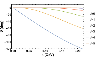
Figure 2: Phase shift of the test potential for the lowest six partial waves.

Table 4: Some numerical values of the phase shift (degrees) at selected values of k (GeV) in Fig. 2.

$\begin{array}[]{ccccc}\hline\cr\hline\cr l&k=0.05&k=0.1&k=0.15&k=0.2\\ 0&-32.2599&-62.9184&-90.5094&-113.833\\ 1&-3.15552&-16.5361&-35.5349&-54.9107\\ 2&-0.101947&-2.22494&-9.5661&-21.2908\\ 3&-0.00173584&-0.160577&-1.61377&-6.08421\\ 4&-0.0000210598&-0.00781134&-0.18254&-1.24548\\ 5&-1.817\times 10^{-7}&-0.000293742&-0.0156874&-0.192916\\ \hline\cr\hline\cr\end{array}$

IV.2 Results and discussion

Since the range of the potential is about 4 fm, a box size of $L=24$ fm is sufficient to make the exponential finite-volume effects negligible. The large volume is for checking purposes in the quantum-mechanical model. We note such a large volume is not accessible in current lattice QCD simulations, although the recent development of the masterfield paradigm makes an important leap in this direction Francis et al. (2020); Fritzsch . To take the continuum limit we use lattices of $20^{3}$ with $a=1.2$ fm, $24^{3}$ with $a=1$ fm, and $30^{3}$ with $a=0.8$ fm for cubic case. For the elongated case we use the same three lattice spacings and the same size $L=24$ fm in the $x$, and $y$ direction but we elongate the $z$ direction by a factor of $\eta=1.5$. The lowest nonzero momentum in the spectrum is controlled by the box size $k_{min}=2\pi/(L\eta)$. For the higher $k$ values the density of states gets higher. We study states with $k<0.2$ GeV. In this $k$-range only the phase shifts for $\ell\leq 5$ are significantly different from zero (see Fig. 2). Therefore, we expect convergence of the QCs by $l=4$ or $l=5$. The total number of noninteracting levels (with or without degeneracies) under the cutoff are summarized in Table 5 for all the cases considered in this work. We see the number of levels is still fairly large after the $k$ cutoff. In such cases, we apply an additional cut of 40 distinct levels to keep the number manageable, which implies a smaller $k$ range. Interactions cannot change the number of levels in our model, only shift them, so the noninteracting levels serve as a useful guide. We provide all the noninteracting levels obtained from kinematics in Sec. 1 of the Supplement Material sup . For the rest frame of cubic and elongated boxes, we see that the levels are more packed in elongated box (36 vs 14), which also reaches lower in the first nonzero level (0.03 vs 0.05 GeV). The ability to reach lower energy can be regarded as an advantage of the elongated geometry over the cubic. The integer indices of lab momentum for each particle along with their degeneracy are shown. We see how the particles are arranged to have back-to-back momenta so the total momentum is zero in both lab and CM frames. Level 9 in cubic box is a special case with accidental degeneracy of 6 from $(\pm 3,0,0)$ and 24 from $(\pm 2,\pm 2,\pm 1)$. Its counterpart in elongated box is level 21, but with a different degeneracy of 4 from $(\pm 3,0,0)$ and 16 from $(\pm 3,\pm 2,\pm 1)$. The one with $(\pm 2,\pm 2,\pm 1)$ is level 20 which has lower energy and degeneracy 8. These $k$ levels are also free-particle poles in the zeta functions in Eqs.(20) and (40). Interactions will cause $k$ to deviate from the free levels. The amount of the deviation is related to phase shifts via the Lüscher QC.

Since the QCs are block diagonalized by irreps, the levels must also be projected into the irreps as discussed earlier. The interacting levels will be given in numerical tables when we study the convergence of QCs. In Fig. 3 we show an example of the projected spectrum for the rest frame in cubic box ($O_{h}$ group). Note that in the noninteracting case levels with the same energy appear in different irreps. Degeneracies in the noninteracting levels are removed by the interactions. The strongest interaction is in the $A_{1g}$ channel which is dominated by $l=0$. The lowest level (zero) is shifted up by about $10$ MeV. The next strongest interaction is the $T_{1u}$ channel which is dominated by $l=1$ where the lowest level is shifted up by about $0.5$ MeV. The shift is upwards across the board because the interaction is repulsive everywhere. The shifts in other channels are barely visible, but can be resolved numerically. As an additional check we repeated the entire procedure, including the continuum extrapolations, with the interactions turned off. We compared these results with the expectation from basic kinematics and found perfect agreement. This also provided us with a straightforward way to determine the multiplicity for each noninteracting level in each irrep.

Table 5: Number of distinct and total noninteracting levels for two spinless particles of unequal masses in a box of geometry $L\times L\times\eta L$ with $L=24$ fm and cutoff $k<0.2$ GeV.

$\begin{array}[]{c | c c | c c }\hline\cr\hline\cr d&\lx@intercol\hfil\text{cubic }(\eta=1)\hfil\lx@intercol\vrule\lx@intercol&\lx@intercol\hfil\text{$z$ elongated }(\eta=1.5)\hfil\lx@intercol\\ \hline\cr&\text{distinct}&\text{total}&\text{distinct}&\text{total}\\ \hline\cr(0,0,0)&14&251&36&359\\ (0,0,1)&54&252&79&367\\ (1,1,0)&73&245&108&355\\ (1,1,1)&54&342&204&363\\ (0,1,2)&107&240&218&366\\ \hline\cr\hline\cr\end{array}$

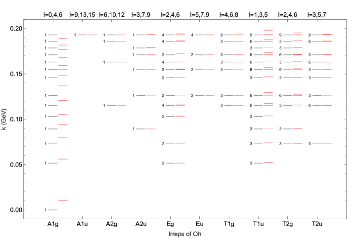
Figure 3: Discrete box levels in the rest frame of cubic box of size $L=24$ fm up to $k=0.2$ GeV. The free-particle (black) and interacting (red) levels are shown side by side for comparison. The numbers next to free levels indicate degeneracy. The box energies are obtained in the lab frame from an extrapolation on several lattices, projected into the irreps of $O_{h}$, then converted to CM momentum $k$. The top labels show the lowest partial waves in each irrep. Numerical values for both noninteracting and interacting levels can be found in Sec. 1 and Sec. 4 of the Supplemental Material sup .

Our objective is to reproduce the finite-volume spectrum using the QCs and the phase shifts. The matrix elements needed to construct the QCs are given in Table 22 and Table LABEL:tab:D4h in Appendix B. Since the symmetry-adapted QC is a single condition that couples to all possible partial waves in a given irrep, we can compute the phase shift from the spectrum only if the lowest partial wave is retained. As an example, we show in Fig. 4 the phase shift prediction for $l=0$ partial wave in the $A_{1g}$ QC by feeding the interacting energy levels into the Lüscher formula. All other cases can be found in Sec. 2 of the Supplemental Material sup . We see the reconstruction is excellent up to $k=0.2$ GeV, but with a notable exception point at $k=0.1548$ GeV (level 9) where the box level seems “incompatible” with the lowest-order Lüscher QC. A feature of the exception is that it happens at a free-particle pole (faint vertical line). We say the level is “pinched” at the free-particle pole. All other points are in between free-particle poles. The discrepancy is due to the fact that we neglected the higher partial waves in the QC.

As a general method to assess the effects of higher partial waves, we investigate the convergence of the QC by feeding it the infinite-volume phase shifts and comparing the resulting levels with the box levels. We find it more convenient to locate the roots of this equation by solving the real valued QC1 rather than the complex valued QC2. After the roots are found from QC1, we pass them through QC2 to double check they are also roots. This is a different approach to Ref.Woss et al. (2020) where QC2 is solved by eigenvalue decomposition for coupled channels. We check the convergence order by order: “order 1” has only the lowest partial wave, “order 2” with the next partial wave added, and so on. In the limit that all the partial waves are included, perfect agreement is expected. In practice, we check convergence for the lowest five partial waves (up to $l=4$), which is adequate for most applications. In some cases, we consider $l=5$. Once convergence is achieved, we consider the QC checked at the given order.

The comparison involves very small differences that are not easily discernible visually. To better gauge the quality of the convergence, we introduce a numerical measure

$$\chi^{2}=\frac{(k_{\rm box}-k_{\rm QC})^{2}}{(k_{\rm box}-k_{\rm lat})^{2}},$$ (60)

where $k_{\rm box}$ is the continuum box level extrapolated from the three lattice spacings, $k_{\rm lat}$ the level on the lattice with the finest lattice spacing, and $k_{\rm QC}$ the solution from the QC at each order. The extrapolation is a function of $a^{6}$, the error present in the Hamiltonian from the seven-point stencil approximation in Eq.(50). We show an example of the continuum extrapolation in Fig. 5. For comparison, we also show the result from the standard three-point stencil approximation Eq.(48) which has $O(a^{2})$ discretization errors. We see that they converge to the same result but at different rates.

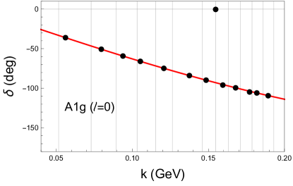
Figure 4: Phase shifts reconstruction for the lowest partial wave ($l=0$) in the $A_{1g}$ irrep of rest frame $d=(0,0,0)$ in cubic box. The black points are the predicted phase shift via Lüscher formula. The red curve is the infinite-volume phase shift. The faint vertical lines correspond to noninteracting levels in the box.

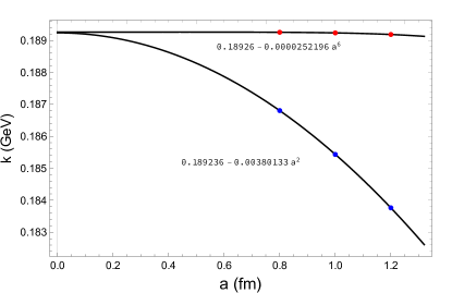
Figure 5: Continuum extrapolation of a level in the $A_{1g}$ irrep of $O_{h}$. Three points are obtained on lattices $20^{3}$ with $a=1.2$ fm, $24^{3}$ with $a=1$ fm, and $30^{3}$ with $a=0.8$ fm. The red points are from the seven-point stencil and the blue points from the three-point stencil. The fitted curves and forms are also displayed.

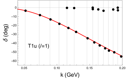
Figure 6: Phase shifts reconstruction for the lowest partial wave ($l=1$) in the $T_{1u}$ irrep of rest frame $d=(0,0,0)$ in cubic box. The black points are the predicted phase shift via Lüscher formula. The red curve is the infinite-volume phase shift. The faint vertical lines correspond to noninteracting levels in the box.

Basically, the convergence is measured against the tiny difference between the continuum box levels and those from the largest lattice used in the extrapolation (about six decimal places, or 1 eV out of 1 MeV). Note that the $\chi^{2}$ introduced is not in the standard sense of curve fitting where the best value is around 1. Here the smaller its value, the better the convergence. This is a highly sensitive measure: nonconvergence of a single level will have a large contribution to the total $\chi^{2}$. In cases of a box level coinciding with a free-particle pole, we indicate it by a red star and replace $k_{\rm QC}$ in Eq.(60) by $k_{\rm free}$.

We apply the method to the $A_{1g}$ example in Fig. 4. The results are given in Table 6. The overall quality of convergence is measured by the total $\chi^{2}$ of all the levels. We see that at order 1 (only $l=0$ $s$ wave is included), it is about 277. The level most responsible for the discrepancy is level 12, followed by levels 10, 9, 4, 6. We note that level 9 is the one that is obscured by the noninteracting energy pole, the one that stands out in Fig. 4. At order 2, the QC is enlarged by adding the next partial wave ($l=4$). We see that the addition of $l=4$ causes small changes in the $k$ values that improves the total $\chi^{2}$. The exception level, level 9, is now approximated well by one of the roots of the QC. The quality is indicated by the small $\chi^{2}$ value of 0.019. In fact, all the levels at order 2 have small $\chi^{2}$, leading to a total of 3.73, much smaller than 277 at order 1. This is a prime example of how the higher partial wave impacts the QC and how we check convergence.

Table 6: The companion table to Fig. 4 for $A_{1g}$, showing convergence of quantization condition by adding higher partial waves. The k levels in GeV are compared directly order by order, using the $\chi^{2}$ measure defined in Eq.(60). The red star indicates that the box level is “pinched” at a free-particle pole.

$\begin{array}[]{ccccccc}\hline\cr\hline\cr\text{Level}&\text{Box L}&\text{Lattice}&\text{Order 1}&\text{Order 2}&\chi^{2}\text{ Order 1}&\chi^{2}\text{ Order 2}\\ \hline\cr 14&0.18926&0.189253&0.189254&0.18926&0.820197&0.00914913\\ 13&0.181804&0.181799&0.181803&0.181803&0.0205124&\ 0.0146576\\ 12&0.177043&0.177041&0.177007&0.177044&174.698&0.0110595\\ 11&0.167873&0.167867&0.167872&0.167874&0.0419179&\ 0.0215601\\ 10&0.159465&0.159461&0.15944&0.159466&29.8119&0.014445\\ 9&0.154755&0.154749&{\color[rgb]{1,0,0}\ast}0.154723&0.154755&29.1192&0.0191184\\ 8&0.148467&0.148466&0.148466&0.148467&0.763934&\ 0.000166674\\ 7&0.137488&0.137487&0.137489&0.137489&0.0251408&\ 0.0252861\\ 6&0.120712&0.120711&0.12071&0.120712&16.368&0.0213916\\ 5&0.105257&0.105256&0.105256&0.105257&4.20346&0.017348\\ 4&0.0938371&0.0938369&0.0938362&0.0938372&18.3015&\ 0.130459\\ 3&0.0796177&0.0796176&0.0796178&0.0796178&0.453209&\ 0.453221\\ 2&0.0560702&0.0560701&0.0560702&0.0560701&0.214519&\ 0.623864\\ 1&0.01025&0.01025&0.0102501&0.0102501&2.36538&2.36787\\ \hline\cr\hline\cr&&&&\text{\bf Total }\bm{\chi}^{2}&{\bf 277.206}&{\bf 3.7296}\\ \end{array}$

Table 7: The companion table to Fig. 6 for $T_{1u}$, showing convergence of quantization condition by adding higher partial waves. The levels are compared directly order by order, using the $\chi^{2}$ measure defined in Eq.(60). The red star indicates that the box level is “pinched” at a free-particle pole.

$\begin{array}[]{ccccccccc}\hline\cr\hline\cr\text{Level}&\text{Box L}&\text{Lattice}&\text{Order 1}&\text{Order 2}&\text{Order 3}&\chi^{2}\text{ Order 1}&\chi^{2}\text{ Order 2}&\chi^{2}\text{ Order 3}\\ \hline\cr 22&0.198249&0.198241&0.198146&0.198245&0.19825&167.097&\ 0.249283&0.0101593\\ 21&0.193217&0.193213&{\color[rgb]{1,0,0}\ast}0.192974&0.193209&0.193221&2998.88&3.71223&0.470423\\ 20&0.192982&0.192978&{\color[rgb]{1,0,0}\ast}0.192974&{\color[rgb]{1,0,0}\ast}0.192974&0.192975&\ 3.26057&3.26057&2.49916\\ 19&0.187618&0.187613&0.187614&0.187615&0.187619&0.747838&0.42273&0.00535232\\ 18&0.186043&0.186039&{\color[rgb]{1,0,0}\ast}0.185954&0.186041&0.186045&389.699&0.356124&0.194373\\ 17&0.179522&0.179521&0.179489&0.179517&0.179522&807.378&17.3011&0.0125204\\ 16&0.173768&0.173763&0.173698&0.173767&0.173769&206.536&0.0359251&0.00582583\\ 15&0.171233&0.171228&{\color[rgb]{1,0,0}\ast}0.171053&0.171231&0.171233&1447.64&0.209609&0.00394721\\ 14&0.165438&0.165434&0.165382&0.165438&0.165439&128.455&0.0154137&0.00520841\\ 13&0.163206&0.163201&{\color[rgb]{1,0,0}\ast}0.163093&0.163204&0.163206&526.933&0.147073&0.0123243\\ 12&0.157179&0.157177&0.157134&0.157178&0.157179&551.783&0.156363&0.00460883\\ 11&0.154856&0.154853&{\color[rgb]{1,0,0}\ast}0.154723&0.154856&0.154857&1267.98&0.0467443&0.00685293\\ 10&0.154726&0.154725&{\color[rgb]{1,0,0}\ast}0.154723&{\color[rgb]{1,0,0}\ast}0.154723&0.154726&\ 6.59657&6.59657&0.0176498\\ 9&0.146868&0.146867&0.14686&0.146867&0.146868&172.894&\ 2.71263&0.0020146\\ 8&0.129339&0.129339&0.129335&0.129339&0.129339&58.3417&\ 0.000653416&0.0113939\\ 7&0.126379&0.126379&{\color[rgb]{1,0,0}\ast}0.126331&0.126379&0.126379&30130.9&0.976735&0.00253806\\ 6&0.11756&0.117559&0.117552&0.11756&0.11756&323.653&\ 0.0133041&0.00803915\\ 5&0.115359&0.115359&{\color[rgb]{1,0,0}\ast}0.115324&0.115359&0.115359&13893.6&0.272455&0.002095\\ 4&0.103734&0.103734&0.10372&0.103734&0.103734&1539.04&\ 0.0089603&0.0024343\\ 3&0.0901719&0.0901719&0.0901658&0.0901719&0.0901719&\ 11790.7&0.0587094&0.0204841\\ 2&0.0740985&0.0740985&0.0740982&0.0740985&0.0740985&\ 27.9224&0.011686&0.0285701\\ 1&0.0520501&0.0520501&0.0520494&0.0520501&0.0520501&\ 836.425&0.0286906&0.0308669\\ \hline\cr\hline\cr&&&&&\text{\bf Total }\bm{\chi}^{2}&{\bf 67276.5}&{\bf 36.5936}&{\bf 3.35684}\\ \end{array}$

Another interesting example is the $T_{1u}$ irrep in cubic box, shown in Fig. 6. It poses two challenges. One is there are numerous exceptions in this channel. The other is that some levels are nearly degenerate. The convergence study is shown in Table 7. This channel is dominated by the $p$ wave, followed by $l=3$ and $l=5$ which also has a twofold multiplicity. At order 1, the numerous exceptions are indicated by the red stars. At order 2, most are fixed by the addition of $l=3$, but two remain pinched (levels 10 and 20). This demonstrates that the neglected $l=3$ partial wave is largely responsible for the exceptions observed at order 1. A closer examination reveals that the two remaining exceptions are part of nearly degenerate pairs. Only one of the two nearly degenerate points (level 11) is a QC solution but the other (level 10) is not. A similar situation holds for another pair of close-by levels: level 21 is a solution but level 20 is not. This hints at possible influence of the next partial wave $l=5$. Indeed, at order 3, the two points are both solutions of the QC and we obtain a spectrum that is in complete agreement with the box spectrum. The convergence is confirmed by the total $\chi^{2}$: from 67277 at order 1, to 37 at order 2, and to 3.4 at order 3.

We have confirmed the convergence of all 45 cases in the same manner, as summarized in Table 8. One point to emphasize is that to get agreement for certain cases we needed to consider QC all the way to order 5. The irreps in question (Nos. 10, 14, 18, 21, 33, 38, 42, 44) are, as expected, the ones that allow the most mixing between partial waves.

Table 8: Summary of the total $\chi^{2}$ measure showing convergence for all QCs discussed in this work. Here $l(n)$ indicates the lowest few partial waves (and multiplicities) that couple to the QC; $N$ is the number of levels under the cutoff of $k=0.2$ GeV or 40 levels. Detailed convergence data for every individual energy level can be found in Sec. 4 of the Supplemental Material sup .

$\begin{array}[]{cccclllllll}\hline\cr\hline\cr\lx@intercol\hfil\text{\bf Cubic box}\hfil\lx@intercol\\ \text{No.}&d&\text{Group}&\text{QC}&l(n)&\text{N}&\text{Order 1}&\text{Order 2}&\text{Order 3}&\text{Order 4}&\text{Order 5}\\ \hline\cr 1&(0,0,0)&O_{h}&A_{1g}&0,4,6,\cdots&14&277.206&3.7296&&&\\ &&&A_{1u}&9,13,15,\cdots&&&&&&\\ &&&A_{2g}&6,10,12,\cdots&&&&&&\\ 2&&&A_{2u}&3,7,9,\cdots&6&0.0458813&&&&\\ 3&&&E_{g}&2,4,6,\cdots&16&2123.07&5.44639&&&\\ 4&&&E_{u}&5,7,9,\cdots&5&0.0546959&&&\\ 5&&&T_{1g}&4,6,8(2),\cdots&9&0.243897&&&&\\ 6&&&T_{1u}&1,3,5(2),\cdots&22&67276.5&36.5936&3.35684&&\\ 7&&&T_{2g}&2,4,6(2),\cdots&16&2485.36&2.70125&&&\\ 8&&&T_{2u}&3,5,7(2),\cdots&14&4.55575&0.267262&&&\\ 10&(0,0,1)&C_{4v}&A_{1}&0,1,2,3,4(2),\cdots&40&4.08008\times 10^{8}&1.06106\times 10^{10}&10175.7&284.022&\ 6.92792\\ 11&&&A_{2}&4,5,6,\cdots&15&7.46202&0.145375&&\\ 12&&&B_{1}&2,3,4,5,\cdots&34&276889.&402.025&5.9668&&\\ 13&&&B_{2}&2,3,4,5,\cdots&27&350956.&779.183&3.84012&&\\ 14&&&E&1,2,3(2),4(2),\cdots&40&1.32751\times 10^{7}&72379.5&514.979&8.21687&\\ 14&(1,1,0)&C_{2v}&A_{1}&0,1,2(2),3(2),4(3),\cdots&40&1.96654\times 10^{8}&4.77126\times 10^{6}&17298.1&190.94&5.34113\\ 15&&&A_{2}&2,3,4(2),5(2),\cdots&40&54211.3&2998.61&3.01327&&\\ 16&&&B_{1}&1,2,3(2),4(2),\cdots&40&2.84806\times 10^{6}&47754.8&241.517&4.62961&\\ 17&&&B_{2}&1,2,3(2),4(2),\cdots&40&9.36978\times 10^{6}&88719.7&308.013&6.28652&\\ 18&(1,1,1)&C_{3v}&A_{1}&0,1,2,3(2),4(2),\cdots&40&9.16556\times 10^{7}&1.09895\times 10^{6}&22260.&115.412&3.53446\\ 19&&&A_{2}&3,4,5,\cdots&26&111.322&0.44229&&&\\ 20&&&E&1,2(2),3(2),4(3),\cdots&40&8.06257\times 10^{6}&23959.&271.289&4.13508&\\ 21&(0,1,2)&C_{1v}&A_{1}&0,1(2),2(3),3(4),4(5),\cdots&40&1.01852\times 10^{8}&993629.&6858.3&17.3429&2.01417\\ 22&&&A_{2}&1,2(2),3(3),4(4),\cdots&40&8.98645\times 10^{6}&37314.8&293.484&3.18387&\\ \hline\cr\lx@intercol\hfil\text{\bf Elongated box}\hfil\lx@intercol\\ \text{No.}&d&\text{Group}&\text{QC}&l(n)&\text{N}&\text{Order 1}&\text{Order 2}&\text{Order 3}&\text{Order 4}&\text{Order 5}\\ \hline\cr 23&(0,0,0)&D_{4h}&A_{1g}&0,2,4(2),5,\cdots&40&4.06688\times 10^{6}&573.449&8.64225&&\\ 24&&&A_{1u}&5,7,9(2),\cdots&9&0.134224&&&&\\ 25&&&A_{2g}&4,6,8(2),\cdots&3&0.00828583&&&&\\ 26&&&A_{2u}&1,3,5(2),7(2),\cdots&34&131946.&16.2795&10.7998&&\\ 27&&&E_{g}&2,4(2),6(3),\cdots&38&2009.93&0.319341&&&\\ 28&&&E_{u}&1,3(2),5(3),\cdots&40&221693.&41.2595&8.52709&&\\ 29&&&B_{1g}&2,4,6(2),8(2),\cdots&27&703.291&11.0395&&&\\ 30&&&B_{1u}&3,5,7(2),9(2),\cdots&17&7.07159&0.168506&&&\\ 31&&&B_{2g}&2,4,6(2),8(2),\cdots&22&2093.46&0.192&&&\\ 32&&&B_{2u}&3,5,7(2),9(2),\cdots&21&2.06599&0.488025&&&\\ 33&(0,0,1)&C_{4v}&A_{1}&0,1,2,3,4(2),\cdots&40&5.70458\times 10^{8}&9.64404\times 10^{6}&14025.4&166.777&\ 11.0137\\ 34&&&A_{2}&4,5,6,\cdots&21&40.092&0.21509&&\\ 35&&&B_{1}&2,3,4,5,\cdots&40&161200.&274.945&5.1077&&\\ 36&&&B_{2}&2,3,4,5,\cdots&39&318459.&845.868&2.82798&&\\ 37&&&E&1,2,3(2),4(2),\cdots&40&1.66366\times 10^{7}&79648.3&353.966&7.28402&\\ 38&(1,1,0)&C_{2v}&A_{1}&0,1,2(2),3(2),4(3),\cdots&40&2.19334\times 10^{8}&3.60527\times 10^{6}&9669.56&99.3024&27.4093\\ 39&&&A_{2}&2,3,4(2),5(2),\cdots&40&34211.4&295.311&0.804797&&\\ 40&&&B_{1}&1,2,3(2),4(2),\cdots&40&2.97904\times 10^{6}&28179.&115.601&6.80754&\\ 41&&&B_{2}&1,2,3(2),4(2),\cdots&40&9.05592\times 10^{6}&71558.8&146.885&18.7042&\\ 42&(1,1,1)&C_{1v}&A_{1}&0,1(2),2(3),3(4),4(5),\cdots&40&5.45564\times 10^{8}&2.89417\times 10^{6}&15983.3&39.1208&8.00598\\ 43&&&A_{2}&1,2(2),3(3),4(4),\cdots&40&6.85779\times 10^{6}&23813.9&69.434&3.24328&\\ 44&(0,1,2)&C_{1v}&A_{1}&0,1(2),2(3),3(4),4(5),\cdots&40&3.79138\times 10^{8}&3.16621\times 10^{6}&6213.69&17.0296&5.34524\\ 45&&&A_{2}&1,2(2),3(3),4(4),\cdots&40&1.27375\times 10^{7}&45256.8&146.374&2.67257&\\ \hline\cr\hline\cr\end{array}$

Finally we want to see that for the “pinched” points if we can exploit the sensitivity to the second partial wave to produce predictions for its phase shift based solely on the energy input. Note that this is not in general possible at other points since the equation at next order involves two phase shifts constrained by a single equation. Solving for the second partial wave from a generic QC at order 2 with no multiplicities, we have

$$\cos\delta_{\rm 2nd}=M_{22}+\frac{|M_{12}|^{2}}{\cos\delta_{\rm 1st}-M_{11}}.$$ (61)

The “pinched” points occur very near the pole where $|M_{11}|\gg 1$ and then we can approximate the equation by setting $\cos\delta_{\rm 1st}=0$ and solve for $\delta_{\rm 2nd}$. Using above-mentioned $A_{1g}$ and $T_{1u}$ as examples, we plot in Fig. 7 $\cos\delta_{\rm 2nd}$ extracted this way for $l=4$ and $l=3$. We see that the exception points discussed in Figs. 4 and 6 fall on the curve for the infinite-volume phase shift of the second partial wave. This suggests that $\delta_{\rm 1st}(k)$ and $\delta_{\rm 2nd}(k)$ can be separately isolated by considering the QC at orders 1 and 2 respectively. The values obtained for $\delta_{\rm 2nd}(k)$ can be further checked by comparing with the predictions from other irreps which have it as the lowest partial wave. These results demonstrate that exception points at the free-particle poles are sensitive to the second partial wave. If such points are encountered in lattice QCD simulations, then they can be either neglected in the prediction of the lowest partial wave, or be utilized to give an estimate for the second partial wave in the QC. The recipe is not fail proof. We see that two exception points in $T_{1u}$ do not fall on the curve. It happens when a nearly degenerate pair (levels 10 and 11, or levels 20 and 21) is pinched at the free-particle poles. It indicates the possible influence of the third partial wave $l=5$ in the QC. Similar trends are observed in elongated box. Additional cases can be found in Sec. 3 of the Supplemental Material sup .

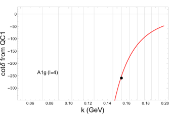
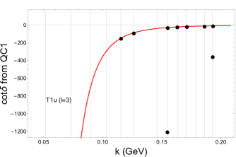
Figure 7: Second partial wave in $A_{1g}$ (top) and $T_{1u}$ (bottom) of cubic box. The black points are $\cos\delta_{\rm 2nd}$ in Eq.(61) with $\cos\delta_{\rm 1st}$ neglected, evaluated at the pinched box levels from order 1. The red curve is the infinite-volume $\cos\delta_{\rm 2nd}$. The faint vertical lines are the free-particle poles.

V Conclusion and outlook

We derived higher-order Lüscher QCs for scattering of two spinless particles of unequal masses. Our results were checked numerically by comparing the QC predictions with the spectrum of two-particle states in a box computed by solving the Schrödinger equation. This is done using a simple potential model in nonrelativistic quantum mechanics. Both the phase shifts in infinite volume and energy levels in finite volume are independently generated in a well-controlled fashion. Here is a summary of our findings.

1. We considered a variety of scenarios: rest frame and four moving frames, cubic and elongated geometries. In total, we examined 22 QCs in cubic box and 23 QCs in elongated box. The five lowest partial waves in each QC are examined. In some cases, up to $l=5$. Matrix elements for all the QCs are given in Appendix B. Some of the QCs are rederived to include higher partial waves, others are new. Generically, we expect the QCs to be valid up to terms which vanish exponentially with the box size.

2. We choose the potential and the box-size so that the systematics associated with finite-volume are negligible, on one hand, and on the other the results are sensitive to partial waves as high as $\ell=5$. This allows us to provide very stringent tests for our results. The numerical checks are done at high precision (to six decimal digits, or differences of 1 eV resolved out of 1 MeV). Up to CM momentum $k=0.2$ GeV and up to 40 levels are examined for each of the QCs. All convergence data, along with noninteracting levels and other information, are provided in the Supplemental Material sup .

3. We found sensitivity to the second lowest partial wave in selected QCs through “pinched” levels which coincide with free-particle poles. The sensitivity can be used to provide an approximate phase shift for the second lowest partial wave despite the presence of the lowest one in a particular channel, but this must be determined on a case by case basis. If such levels are encountered in lattice QCD simulations, they can be either ignored or used to estimate the second partial wave.

4. For the most part, we find elongated boxes work just as well as cubic ones. This bodes well for using elongated boxes as a cost-effective way of varying the kinematic range with a modest increase in the lattice volume.

5. Boosting of the two-particle system in both cubic and elongated boxes allows lower energies to be accessed, thus a wider coverage. We considered four basic types of moving frames $d=(0,0,1)$, $(1,1,0)$, $(1,1,1)$, and $(0,1,2)$. Rules for going higher in momentum are given in Table 1. The trade-off for lower energy is the loss of parity which means more mixing of partial waves.

6. The effort is already paying dividends. For example, we checked the integer-$J$ QCs in Ref. Gockeler et al. (2012) for $d=(1,1,0)$ and $d=(1,1,1)$ and found agreement with ours, despite having different forms due to different basis vectors. Those QCs are only given for up to $l=2$. Here we extend up to $l=4$. We also checked against $C_{3v}$ up to $l=4$ from an independent source Morningstar (2021) and found agreement. We also found a few typos in the QCs included in Ref. Lee and Alexandru (2017). We also checked against all the expressions up to $l=4$ for spinless particles of equal mass at total zero momentum in nonelongated boxes given in Ref. Lüscher (1991) by setting $m_{1}=m_{2}$ in our expressions and found agreement.

7. The numerical check is designed to be transparent and computationally inexpensive. The entire calculation can be done on a laptop.

For outlook, we envision the following possibilities.

1. The QCs can only be used to extract phase shifts from energy only for the lowest partial waves in each irrep. The predictions are affected by cutting off all the higher partial waves. The severity is not known a priori and it depends on the box geometry and the total momentum of the state. The problem can be turned on its head: can we extract the higher partial waves by considering multiple QCs simultaneously? We have seen in limited cases that higher partial waves can be isolated in a single QC despite the presence of a lower one. Is there a systematic approach, taking advantage of multiple irreps, moving frames, and box size? Thus far this was done using various parametrizations of the scattering amplitude.

2. Our results are based on a simple repulsive Gaussian potential. This was appropriate for our goal here, which was to check our derivation of the quantization conditions. We note that the same methodology could be easily applied for other potentials, if there is a physical problem that requires calculation of the two-particle spectrum in a finite box. Any interaction potential can be used in this approach, including potentials given in numerical form or nonlocal potentials $V(r,\bm{p})$ where $\bm{p}$ can be treated as finite differences on the lattice. We note also that the QCs are general to any spinless two-body system below the inelastic threshold in finite volume, not just those relevant to nuclear and particle physics.

3. The formalism can be used to study the finite-volume effects in lattice QCD simulation of physical systems, such as the the magnitude of exponential finite-volume effects ignored by the QCs by considering a smaller box (3.5 to 6 fm); the effect of the range of the model potential; and/or the finite-volume spectrum in the presence of shallow bound states. Even using the naïve $O(a^{2})$ discretization to study the influence of cutoff effects on the extracted finite-volume energies could be interesting.

4. The formalism can be applied with minimal modification to systems with two integer spins. The same is true for two spin-1/2 particles, such as nucleon-nucleon scattering. There is a plethora of NN interaction potentials to work with.

5. Another direction is the extension to systems with total half-integer $J$, such as a spin-0 particle and a spin-1/2 particle. Important physical systems can be studied, a classic example being the delta resonance in pion-nucleon scattering. This is more challenging. Group theory for double-cover groups are involved for half-integer total angular momentum. The QCs for half-integer $J$ should also be checked since they are even more involved than the ones for integer spin. For this case the Hamiltonian must be modified to include spin-orbit coupling. The spin-orbit interaction has been studied in the continuum but finite-volume using a Fourier basis approach Lee et al. (2020). A demonstration on the lattice like the one in this work would be desirable.

Appendix A Group theory details

The different scenarios discussed in the main text are classified by their symmetries which can be treated systematically by group theory. In this appendix, we provide a reasonably self-contained description of the group theoretic ingredients needed in this work.

A.1 Cubic box

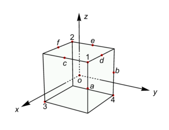
Figure 8: The 24 symmetry operations that form the octahedral group $O$ in cubic box. They are divided into five conjugacy classes: the identity ($\mathbb{E}$); six $\pi/2$ rotations about the three axes (6$C_{4}$); three $\pi$ rotations about the three axes (3$C_{2}$); eight $2\pi/3$ rotations about four body diagonals denoted by 1, 2, 3, 4 (8$C_{3}$); and six $\pi$ rotations about axes parallel to six face diagonals denoted by $a,b,c,d,e,f$ (6$C^{\prime}_{2}$). The operations are performed in a right-hand way with the thumb pointing from the center to the various symmetry points.

For cubic lattices, the symmetry is depicted in Fig. 8. The symmetry group is called the octahedral point group $O$ is a finite subgroup of the continuum rotation group $SO(3)$. It has 24 elements and 5 irreps commonly called $A_{1}$, $A_{2}$, $E$, $T_{1}$, and $T_{2}$ having the respective dimensonality 1,1,2,3, and 3. The $O$ group is sufficient in describing integral angular momentum in cubic box. For half-integral angular momentum, its double-covered group ${}^{2}O$ is needed. It is a general group property that the number of irreps is equal to the number of conjugacy classes. Another property is that the square of irrep dimensions sum to the total number of elements.

For systems at rest, parity (space inversion) is another symmetry in the box. In this case we need the symmetry group $O_{h}=O\otimes\{\mathbb{E},I\}$ which is a direct product with the inversion group (two elements: identity $\mathbb{E}$ and the inversion operation $i$). The $O_{h}$ group has 48 elements and 10 irreps that split into two branches: five with even parity labeled by a plus sign (or g for gerade), five with odd parity labeled by a minus sign (or u for ungerade). Full details of the $O_{h}$ group are given in Table 9. The original $O$ group is embedded in the upper left quadrant of the table. The table shows how to construct $O_{h}$ from $O$. First, double the number of elements by adding a copy of $O$ to the bottom, labelling them as $I1$ to $I24$ so they have one to one correspondence with the original. The new elements can also be named by adding the letter $I$ in front of the original names. For example, $C_{2z}$ to $IC_{2z}$, or one can use the traditional name $\sigma_{z}$ to signify a mirror reflection (rotation about z axis by $\pi/2$ followed by space inversion). Second, double the number of irrep columns by adding a copy to the right, rename the original as ($A_{1g}$, $A_{2g}$, $E_{g}$, $T_{1g}$, $T_{2g}$) and the new ones as ($A_{1u}$, $A_{2u}$, $E_{u}$, $T_{1u}$, and $T_{2u}$). Third, change the sign of the rotation matrices $S_{k}$ and the representations in the added rows. The rotations in the added rows are also known as improper rotations because the operations also include inversion. One way to tell whether a rotation matrix is proper or improper is by its determinant: a proper one has $\det[S]=1$, an improper one $\det[S]=-1$. The $\bm{n}$, $\omega$, and $\{\alpha,\beta,\gamma\}$ columns stay the same. This is practically what it means by $O_{h}=O\otimes\{\mathbb{E},I\}$.

Operationally, the representations for the $O$ group are as follows. $A_{1}$ is the trivial representation, that assigns $1$ to every group element. The $T_{1}$ is the three-dimensional representation corresponding to the transformations of vector ($x,y,z$) under rotations whose matrices are generated via

$$t_{k}=e^{-i(\bm{n}\cdot\bm{J})\omega_{k}},\quad k=1,\cdots,24,$$ (62)

where $(J_{k})_{ij}=i\epsilon_{ijk}$. For the remaining irreps, a sign change in the character of elements 13 to 24 connects $A_{2}$ to $A_{1}$, $T_{2}$ to $T_{1}$, respectively. The $E$ is a real valued, two-dimensional irrep whose matrices can be obtained from the fact that it has Cartesian basis vectors $\sqrt{3}(x^{2}-y^{2})$ and $2z^{2}-x^{2}-y^{2}$. The five distinct matrices in the table are given by Lee and Alexandru (2017).

$$\begin{split}&e_{1}=\left(\begin{array}[]{cc}-1&0\\ 0&1\\ \end{array}\right),e_{2}=\left(\begin{array}[]{cc}-\frac{1}{2}&-\frac{\sqrt{3}}{2}\\ \frac{\sqrt{3}}{2}&-\frac{1}{2}\\ \end{array}\right),e_{3}=\left(\begin{array}[]{cc}-\frac{1}{2}&\frac{\sqrt{3}}{2}\\ -\frac{\sqrt{3}}{2}&-\frac{1}{2}\\ \end{array}\right),\\ &e_{4}=\left(\begin{array}[]{cc}\frac{1}{2}&-\frac{\sqrt{3}}{2}\\ -\frac{\sqrt{3}}{2}&-\frac{1}{2}\\ \end{array}\right),e_{5}=\left(\begin{array}[]{cc}\frac{1}{2}&\frac{\sqrt{3}}{2}\\ \frac{\sqrt{3}}{2}&-\frac{1}{2}\\ \end{array}\right).\end{split}$$ (63)

The character table is implied in the table: for one-dimensional irreps character is simply 1 or -1; for multidimensional irreps character is the trace of the representation matrix. Note that the rotation angle $\omega$ is defined over $4\pi$ and the Euler angles over $0\leq\alpha<2\pi$, $0\leq\beta\leq\pi$, $0\leq\gamma<4\pi$, supplemented by the condition that $\alpha=0$ when $\beta=0$ or $\pi$ (see Chen et al. (2002); Lee and Alexandru (2017)). This matters when double groups are involved. For the single groups considered in this work, they are equivalent to the traditional Euler angles defined over $2\pi$. For notational purposes, we denote the operation matrices by $S_{k}$ and the representation matrices by $D^{\Gamma}(g)$ for irrep $\Gamma$. Note that $S_{k}$ and $D^{T_{1u}}(k)$ happen to coincide for the $O$ group. The full content of the table is used for various aspects to be discussed below.

There are more systematic ways of finding the representation matrices for the irreducible representations in a finite group. One way is to use the multiplication table for the group (see for example Ref. Morningstar et al. (2013)). Another way is known as the Dixon method Dixon (1970). A complete set of irreducible unitary representations can be constructed from a single faithful representation. The method is fairly general: it can find how many conjugacy classes (irreps) and with what dimensionality a new group has, along with its representation matrices. The algorithm is much simpler if the number of irreps and the dimensionalities are known, as is the case for the point groups considered in this work. We applied the simpler version to find the representations in a few cases, taking the $3\times 3$ rotation matrices of group elements as a faithful representation. After the representation matrices are found, character tables and multiplication tables can be constructed and compared with published versions as a cross check.

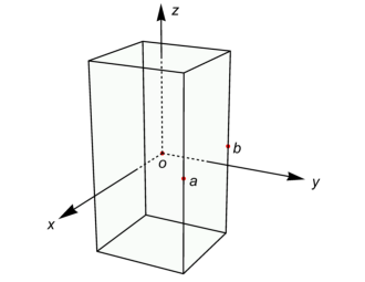
Figure 9: The eight symmetry operations that form the dihedral group $D_{4}$ in elongated box whose dimensions are $L\times L\times\eta L$ where $\eta$ is the elongation factor in the $z$ direction. They are divided into five conjugacy classes: the identity ($\mathbb{E}$), two $\pi/2$ rotations about the $z$ axis (2$C_{4}$), one $\pi$ rotation about the $z$ axis ($C_{2}$), two $\pi$ rotations about $x$ and $y$ axes (2$C^{\prime}_{2}$), and two $\pi$ rotations about the two diagonals in the $xy$ plane denoted by $Oa$ and $Ob$ (2$C^{\prime\prime}_{2}$).

Table 9: Group table of $O_{h}$ for rest frame in cubic box. The inversion is labeled by preceding with the letter $I$ in the $k$ and $O_{h}$ columns. The matrices $e_{k}$, $t_{k}$ are discussed in the text.

$\begin{array}[]{c | c c c c c c c c c c | c c c c c}\hline\cr\hline\cr k&O_{h}&\bm{n}&\omega&S_{k}&\{\alpha,\beta,\gamma\}&A_{1g}&A_{2g}&E_{g}&T_{1g}&T_{2g}&A_{1u}&A_{2u}&E_{u}&T_{1u}&T_{2u}\\ \hline\cr 1&\mathbb{E}&\{0,0,1\}&4\pi&t_{1}&\{0,0,0\}&1&1&\mathds{1}&t_{1}&t_{1}&1&1&\mathds{1}&t_{1}&t_{1}\\ 2&C_{2x}&\{1,0,0\}&\pi&t_{2}&\{0,\pi,\pi\}&1&1&\mathds{1}&t_{2}&t_{2}&1&1&\mathds{1}&t_{2}&t_{2}\\ 3&C_{2y}&\{0,1,0\}&\pi&t_{3}&\{0,\pi,0\}&1&1&\mathds{1}&t_{3}&t_{3}&1&1&\mathds{1}&t_{3}&t_{3}\\ 4&C_{2z}&\{0,0,1\}&\pi&t_{4}&\{0,0,\pi\}&1&1&\mathds{1}&t_{4}&t_{4}&1&1&\mathds{1}&t_{4}&t_{4}\\ 5&C_{31}^{+}&\{1,1,1\}&\frac{2\pi}{3}&t_{5}&\left\{0,\frac{\pi}{2},\frac{\pi}{2}\right\}&1&1&e_{3}&t_{5}&t_{5}&1&1&e_{3}&t_{5}&t_{5}\\ 6&C_{32}^{+}&\{-1,-1,1\}&\frac{2\pi}{3}&t_{6}&\left\{\pi,\frac{\pi}{2},\frac{7\pi}{2}\right\}&1&1&e_{3}&t_{6}&t_{6}&1&1&e_{3}&t_{6}&t_{6}\\ 7&C_{33}^{+}&\{1,-1,-1\}&\frac{2\pi}{3}&t_{7}&\left\{\pi,\frac{\pi}{2},\frac{5\pi}{2}\right\}&1&1&e_{3}&t_{7}&t_{7}&1&1&e_{3}&t_{7}&t_{7}\\ 8&C_{34}^{+}&\{-1,1,-1\}&\frac{2\pi}{3}&t_{8}&\left\{0,\frac{\pi}{2},\frac{7\pi}{2}\right\}&1&1&e_{3}&t_{8}&t_{8}&1&1&e_{3}&t_{8}&t_{8}\\ 9&C_{31}^{-}&\{1,1,1\}&\frac{10\pi}{3}&t_{9}&\left\{\frac{\pi}{2},\frac{\pi}{2},3\pi\right\}&1&1&e_{2}&t_{9}&t_{9}&1&1&e_{2}&t_{9}&t_{9}\\ 10&C_{32}^{-}&\{-1,-1,1\}&\frac{10\pi}{3}&t_{10}&\left\{\frac{3\pi}{2},\frac{\pi}{2},2\pi\right\}&1&1&e_{2}&t_{10}&t_{10}&1&1&e_{2}&t_{10}&t_{10}\\ 11&C_{33}^{-}&\{1,-1,-1\}&\frac{10\pi}{3}&t_{11}&\left\{\frac{\pi}{2},\frac{\pi}{2},0\right\}&1&1&e_{2}&t_{11}&t_{11}&1&1&e_{2}&t_{11}&t_{11}\\ 12&C_{34}^{-}&\{-1,1,-1\}&\frac{10\pi}{3}&t_{12}&\left\{\frac{3\pi}{2},\frac{\pi}{2},3\pi\right\}&1&1&e_{2}&t_{12}&t_{12}&1&1&e_{2}&t_{12}&t_{12}\\ 13&C_{4x}^{+}&\{1,0,0\}&\frac{\pi}{2}&t_{13}&\left\{\frac{3\pi}{2},\frac{\pi}{2},\frac{5\pi}{2}\right\}&1&-1&e_{4}&t_{13}&-t_{13}&1&-1&e_{4}&t_{13}&-t_{13}\\ 14&C_{4y}^{+}&\{0,1,0\}&\frac{\pi}{2}&t_{14}&\left\{0,\frac{\pi}{2},0\right\}&1&-1&e_{5}&t_{14}&-t_{14}&1&-1&e_{5}&t_{14}&-t_{14}\\ 15&C_{4z}^{+}&\{0,0,1\}&\frac{\pi}{2}&t_{15}&\left\{0,0,\frac{\pi}{2}\right\}&1&-1&e_{1}&t_{15}&-t_{15}&1&-1&e_{1}&t_{15}&-t_{15}\\ 16&C_{4x}^{-}&\{1,0,0\}&\frac{7\pi}{2}&t_{16}&\left\{\frac{\pi}{2},\frac{\pi}{2},\frac{7\pi}{2}\right\}&1&-1&e_{4}&t_{16}&-t_{16}&1&-1&e_{4}&t_{16}&-t_{16}\\ 17&C_{4y}^{-}&\{0,1,0\}&\frac{7\pi}{2}&t_{17}&\left\{\pi,\frac{\pi}{2},3\pi\right\}&1&-1&e_{5}&t_{17}&-t_{17}&1&-1&e_{5}&t_{17}&-t_{17}\\ 18&C_{4z}^{-}&\{0,0,1\}&\frac{7\pi}{2}&t_{18}&\left\{0,0,\frac{7\pi}{2}\right\}&1&-1&e_{1}&t_{18}&-t_{18}&1&-1&e_{1}&t_{18}&-t_{18}\\ 19&C_{2a}&\{1,1,0\}&\pi&t_{19}&\left\{0,\pi,\frac{\pi}{2}\right\}&1&-1&e_{1}&t_{19}&-t_{19}&1&-1&e_{1}&t_{19}&-t_{19}\\ 20&C_{2b}&\{-1,1,0\}&\pi&t_{20}&\left\{0,\pi,\frac{7\pi}{2}\right\}&1&-1&e_{1}&t_{20}&-t_{20}&1&-1&e_{1}&t_{20}&-t_{20}\\ 21&C_{2c}&\{1,0,1\}&\pi&t_{21}&\left\{0,\frac{\pi}{2},\pi\right\}&1&-1&e_{5}&t_{21}&-t_{21}&1&-1&e_{5}&t_{21}&-t_{21}\\ 22&C_{2d}&\{0,1,1\}&\pi&t_{22}&\left\{\frac{\pi}{2},\frac{\pi}{2},\frac{\pi}{2}\right\}&1&-1&e_{4}&t_{22}&-t_{22}&1&-1&e_{4}&t_{22}&-t_{22}\\ 23&C_{2e}&\{-1,0,1\}&\pi&t_{23}&\left\{\pi,\frac{\pi}{2},0\right\}&1&-1&e_{5}&t_{23}&-t_{23}&1&-1&e_{5}&t_{23}&-t_{23}\\ 24&C_{2f}&\{0,-1,1\}&\pi&t_{24}&\left\{\frac{3\pi}{2},\frac{\pi}{2},\frac{7\pi}{2}\right\}&1&-1&e_{4}&t_{24}&-t_{24}&1&-1&e_{4}&t_{24}&-t_{24}\\ \hline\cr I1&I\mathbb{E}&\{0,0,1\}&4\pi&-t_{1}&\{0,0,0\}&1&1&\mathds{1}&t_{1}&t_{1}&-1&-1&-\mathds{1}&-t_{1}&-t_{1}\\ I2&IC_{2x}&\{1,0,0\}&\pi&-t_{2}&\{0,\pi,\pi\}&1&1&\mathds{1}&t_{2}&t_{2}&-1&-1&-\mathds{1}&-t_{2}&-t_{2}\\ I3&IC_{2y}&\{0,1,0\}&\pi&-t_{3}&\{0,\pi,0\}&1&1&\mathds{1}&t_{3}&t_{3}&-1&-1&-\mathds{1}&-t_{3}&-t_{3}\\ I4&IC_{2z}&\{0,0,1\}&\pi&-t_{4}&\{0,0,\pi\}&1&1&\mathds{1}&t_{4}&t_{4}&-1&-1&-\mathds{1}&-t_{4}&-t_{4}\\ I5&IC_{31}^{+}&\{1,1,1\}&\frac{2\pi}{3}&-t_{5}&\left\{0,\frac{\pi}{2},\frac{\pi}{2}\right\}&1&1&e_{3}&t_{5}&t_{5}&-1&-1&-e_{3}&-t_{5}&-t_{5}\\ I6&IC_{32}^{+}&\{-1,-1,1\}&\frac{2\pi}{3}&-t_{6}&\left\{\pi,\frac{\pi}{2},\frac{7\pi}{2}\right\}&1&1&e_{3}&t_{6}&t_{6}&-1&-1&-e_{3}&-t_{6}&-t_{6}\\ I7&IC_{33}^{+}&\{1,-1,-1\}&\frac{2\pi}{3}&-t_{7}&\left\{\pi,\frac{\pi}{2},\frac{5\pi}{2}\right\}&1&1&e_{3}&t_{7}&t_{7}&-1&-1&-e_{3}&-t_{7}&-t_{7}\\ I8&IC_{34}^{+}&\{-1,1,-1\}&\frac{2\pi}{3}&-t_{8}&\left\{0,\frac{\pi}{2},\frac{7\pi}{2}\right\}&1&1&e_{3}&t_{8}&t_{8}&-1&-1&-e_{3}&-t_{8}&-t_{8}\\ I9&IC_{31}^{-}&\{1,1,1\}&\frac{10\pi}{3}&-t_{9}&\left\{\frac{\pi}{2},\frac{\pi}{2},3\pi\right\}&1&1&e_{2}&t_{9}&t_{9}&-1&-1&-e_{2}&-t_{9}&-t_{9}\\ I10&IC_{32}^{-}&\{-1,-1,1\}&\frac{10\pi}{3}&-t_{10}&\left\{\frac{3\pi}{2},\frac{\pi}{2},2\pi\right\}&1&1&e_{2}&t_{10}&t_{10}&-1&-1&-e_{2}&-t_{10}&-t_{10}\\ I11&IC_{33}^{-}&\{1,-1,-1\}&\frac{10\pi}{3}&-t_{11}&\left\{\frac{\pi}{2},\frac{\pi}{2},0\right\}&1&1&e_{2}&t_{11}&t_{11}&-1&-1&-e_{2}&-t_{11}&-t_{11}\\ I12&IC_{34}^{-}&\{-1,1,-1\}&\frac{10\pi}{3}&-t_{12}&\left\{\frac{3\pi}{2},\frac{\pi}{2},3\pi\right\}&1&1&e_{2}&t_{12}&t_{12}&-1&-1&-e_{2}&-t_{12}&-t_{12}\\ I13&IC_{4x}^{+}&\{1,0,0\}&\frac{\pi}{2}&-t_{13}&\left\{\frac{3\pi}{2},\frac{\pi}{2},\frac{5\pi}{2}\right\}&1&-1&e_{4}&t_{13}&-t_{13}&-1&1&-e_{4}&-t_{13}&t_{13}\\ I14&IC_{4y}^{+}&\{0,1,0\}&\frac{\pi}{2}&-t_{14}&\left\{0,\frac{\pi}{2},0\right\}&1&-1&e_{5}&t_{14}&-t_{14}&-1&1&-e_{5}&-t_{14}&t_{14}\\ I15&IC_{4z}^{+}&\{0,0,1\}&\frac{\pi}{2}&-t_{15}&\left\{0,0,\frac{\pi}{2}\right\}&1&-1&e_{1}&t_{15}&-t_{15}&-1&1&-e_{1}&-t_{15}&t_{15}\\ I16&IC_{4x}^{-}&\{1,0,0\}&\frac{7\pi}{2}&-t_{16}&\left\{\frac{\pi}{2},\frac{\pi}{2},\frac{7\pi}{2}\right\}&1&-1&e_{4}&t_{16}&-t_{16}&-1&1&-e_{4}&-t_{16}&t_{16}\\ I17&IC_{4y}^{-}&\{0,1,0\}&\frac{7\pi}{2}&-t_{17}&\left\{\pi,\frac{\pi}{2},3\pi\right\}&1&-1&e_{5}&t_{17}&-t_{17}&-1&1&-e_{5}&-t_{17}&t_{17}\\ I18&IC_{4z}^{-}&\{0,0,1\}&\frac{7\pi}{2}&-t_{18}&\left\{0,0,\frac{7\pi}{2}\right\}&1&-1&e_{1}&t_{18}&-t_{18}&-1&1&-e_{1}&-t_{18}&t_{18}\\ I19&IC_{2a}&\{1,1,0\}&\pi&-t_{19}&\left\{0,\pi,\frac{\pi}{2}\right\}&1&-1&e_{1}&t_{19}&-t_{19}&-1&1&-e_{1}&-t_{19}&t_{19}\\ I20&IC_{2b}&\{-1,1,0\}&\pi&-t_{20}&\left\{0,\pi,\frac{7\pi}{2}\right\}&1&-1&e_{1}&t_{20}&-t_{20}&-1&1&-e_{1}&-t_{20}&t_{20}\\ I21&IC_{2c}&\{1,0,1\}&\pi&-t_{21}&\left\{0,\frac{\pi}{2},\pi\right\}&1&-1&e_{5}&t_{21}&-t_{21}&-1&1&-e_{5}&-t_{21}&t_{21}\\ I22&IC_{2d}&\{0,1,1\}&\pi&-t_{22}&\left\{\frac{\pi}{2},\frac{\pi}{2},\frac{\pi}{2}\right\}&1&-1&e_{4}&t_{22}&-t_{22}&-1&1&-e_{4}&-t_{22}&t_{22}\\ I23&IC_{2e}&\{-1,0,1\}&\pi&-t_{23}&\left\{\pi,\frac{\pi}{2},0\right\}&1&-1&e_{5}&t_{23}&-t_{23}&-1&1&-e_{5}&-t_{23}&t_{23}\\ I24&C_{2f}&\{0,-1,1\}&\pi&-t_{24}&\left\{\frac{3\pi}{2},\frac{\pi}{2},\frac{7\pi}{2}\right\}&1&-1&e_{4}&t_{24}&-t_{24}&-1&1&-e_{4}&-t_{24}&t_{24}\\ \hline\cr\hline\cr\end{array}$

Table 10: Group table of $D_{4h}$ for rest frame in elongated box. The inversion is labeled by preceding with the letter $I$ in the $k$ and $O_{h}$ columns. The representations of $E$ are given in terms of Pauli matrices.

$\begin{array}[]{c | c c c c c c c c c c | c c c c c}\hline\cr\hline\cr k&D_{4h}&\bm{n}&\omega&S_{k}&\{\alpha,\beta,\gamma\}&A_{1g}&A_{2g}&B_{1g}&B_{2g}&E_{g}&A_{1u}&A_{2u}&B_{1u}&B_{2u}&E_{u}\\ \hline\cr 1&\mathbb{E}&\{0,0,1\}&4\pi&t_{1}&\{0,0,0\}&1&1&1&1&\mathds{1}&1&1&1&1&\mathds{1}\\ 2&C_{4z}^{+}&\{0,0,1\}&\frac{\pi}{2}&t_{15}&\left\{0,0,\frac{\pi}{2}\right\}&1&1&-1&-1&-i\sigma_{2}&1&1&-1&-1&-i\sigma_{2}\\ 3&C_{4z}^{-}&\{0,0,1\}&\frac{7\pi}{2}&t_{18}&\left\{0,0,\frac{7\pi}{2}\right\}&1&1&-1&-1&i\sigma_{2}&1&1&-1&-1&i\sigma_{2}\\ 4&C_{2z}&\{0,0,1\}&\pi&t_{4}&\{0,0,\pi\}&1&1&1&1&-\mathds{1}&1&1&1&1&-\mathds{1}\\ 5&C_{2x}&\{1,0,0\}&\pi&t_{2}&\{0,\pi,\pi\}&1&-1&1&-1&\sigma_{3}&1&-1&1&-1&\sigma_{3}\\ 6&C_{2y}&\{0,1,0\}&\pi&t_{3}&\{0,\pi,0\}&1&-1&1&-1&-\sigma_{3}&1&-1&1&-1&-\sigma_{3}\\ 7&C_{2a}&\{1,1,0\}&\pi&t_{19}&\left\{0,\pi,\frac{\pi}{2}\right\}&1&-1&-1&1&\sigma_{1}&1&-1&-1&1&\sigma_{1}\\ 8&C_{2b}&\{-1,1,0\}&\pi&t_{20}&\left\{0,\pi,\frac{7\pi}{2}\right\}&1&-1&-1&1&-\sigma_{1}&1&-1&-1&1&-\sigma_{1}\\ \hline\cr I1&I\mathbb{E}&\{0,0,1\}&4\pi&-t_{1}&\{0,0,0\}&1&1&1&1&\mathds{1}&-1&-1&-1&-1&-\mathds{1}\\ I2&IC_{4z}^{+}&\{0,0,1\}&\frac{\pi}{2}&-t_{15}&\left\{0,0,\frac{\pi}{2}\right\}&1&1&-1&-1&-i\sigma_{2}&-1&-1&1&1&i\sigma_{2}\\ I3&IC_{4z}^{-}&\{0,0,1\}&\frac{7\pi}{2}&-t_{18}&\left\{0,0,\frac{7\pi}{2}\right\}&1&1&-1&-1&i\sigma_{2}&-1&-1&1&1&-i\sigma_{2}\\ I4&IC_{2z}&\{0,0,1\}&\pi&-t_{4}&\{0,0,\pi\}&1&1&1&1&-\mathds{1}&-1&-1&-1&-1&\mathds{1}\\ I5&IC_{2x}&\{1,0,0\}&\pi&-t_{2}&\{0,\pi,\pi\}&1&-1&1&-1&\sigma_{3}&-1&1&-1&1&-\sigma_{3}\\ I6&IC_{2y}&\{0,1,0\}&\pi&-t_{3}&\{0,\pi,0\}&1&-1&1&-1&-\sigma_{3}&-1&1&-1&1&\sigma_{3}\\ I7&IC_{2a}&\{1,1,0\}&\pi&-t_{19}&\left\{0,\pi,\frac{\pi}{2}\right\}&1&-1&-1&1&\sigma_{1}&-1&1&1&-1&-\sigma_{1}\\ I8&IC_{2b}&\{-1,1,0\}&\pi&-t_{20}&\left\{0,\pi,\frac{7\pi}{2}\right\}&1&-1&-1&1&-\sigma_{1}&-1&1&1&-1&\sigma_{1}\\ \hline\cr\hline\cr\end{array}$

Table 11: Group table of $C_{4v}$ for moving frame $d=(0,0,1)$ in both cubic and elongated boxes. The corresponding elements in $O_{h}$ and $D_{4h}$ that preserve the direction are indicated.

$\begin{array}[]{ccccccccccc}\hline\cr\hline\cr C_{4v}&O_{h}&D_{4h}&\bm{n}&\omega&\{\alpha,\beta,\gamma\}&A_{1}&A_{2}&B_{1}&B_{2}&E\\ \hline\cr\mathbb{E}&1&1&\{0,0,1\}&4\pi&\{0,0,0\}&1&1&1&1&\mathcal{I}\\ C_{2z}&4&4&\{0,0,1\}&\pi&\{0,0,\pi\}&1&1&1&1&-\mathcal{I}\\ C_{4z}^{+}&15&2&\{0,0,1\}&\frac{\pi}{2}&\left\{0,0,\frac{\pi}{2}\right\}&1&1&-1&-1&i\sigma_{2}\\ C_{4z}^{-}&18&3&\{0,0,1\}&\frac{7\pi}{2}&\left\{0,0,\frac{7\pi}{2}\right\}&1&1&-1&-1&-i\sigma_{2}\\ IC_{2x}&I2&I5&\{1,0,0\}&\pi&\{0,\pi,\pi\}&1&-1&1&-1&\sigma_{3}\\ IC_{2y}&I3&I6&\{0,1,0\}&\pi&\{0,\pi,0\}&1&-1&1&-1&-\sigma_{3}\\ IC_{2a}&I19&I7&\{1,1,0\}&\pi&\left\{0,\pi,\frac{\pi}{2}\right\}&1&-1&-1&1&-\sigma_{1}\\ IC_{2b}&I20&I8&\{-1,1,0\}&\pi&\left\{0,\pi,\frac{7\pi}{2}\right\}&1&-1&-1&1&\sigma_{1}\\ \hline\cr\hline\cr\end{array}$

Table 12: Group table of $C_{3v}$ for moving frame $d=(1,1,1)$ in cubic box only. The corresponding elements in $O_{h}$ that preserve the direction are indicated. This moving frame is not allowed in $z$ elongated box.

$\begin{array}[]{ccccccccc}\hline\cr\hline\cr C_{3v}&O_{h}&\bm{n}&\omega&\{\alpha,\beta,\gamma\}&A_{1}&A_{2}&E\\ \hline\cr\mathbb{E}&1&\{0,0,1\}&4\pi&\{0,0,0\}&1&1&\mathcal{I}\\ C_{31}^{+}&5&\{1,1,1\}&\frac{2\pi}{3}&\left\{0,\frac{\pi}{2},\frac{\pi}{2}\right\}&1&1&\frac{1}{2}\left(-\mathcal{I}+i\sqrt{3}\sigma_{2}\right)\\ C_{31}^{-}&9&\{1,1,1\}&\frac{10\pi}{3}&\left\{\frac{\pi}{2},\frac{\pi}{2},3\pi\right\}&1&1&\frac{1}{2}\left(-\mathcal{I}-i\sqrt{3}\sigma_{2}\right)\\ IC_{2b}&I20&\{-1,1,0\}&\pi&\left\{0,\pi,\frac{7\pi}{2}\right\}&1&-1&\frac{1}{2}\left(\sigma_{3}-\sqrt{3}\sigma_{1}\right)\\ IC_{2e}&I23&\{-1,0,1\}&\pi&\left\{\pi,\frac{\pi}{2},0\right\}&1&-1&-\sigma_{3}\\ IC_{2f}&I24&\{0,-1,1\}&\pi&\left\{\frac{3\pi}{2},\frac{\pi}{2},\frac{7\pi}{2}\right\}&1&-1&\frac{1}{2}\left(\sqrt{3}\sigma_{1}+\sigma_{3}\right)\\ \hline\cr\hline\cr\end{array}$

Table 13: Group table of $C_{2v}$ for moving frame $d=(1,1,0)$ in both cubic and elongated boxes. The corresponding elements in $O_{h}$ and $D_{4h}$ that preserve the direction are indicated.

$\begin{array}[]{cccccccccc}\hline\cr\hline\cr C_{2v}&O_{h}&D_{4h}&\bm{n}&\omega&\{\alpha,\beta,\gamma\}&A_{1}&A_{2}&B_{1}&B_{2}\\ \hline\cr\mathbb{E}&1&1&\{0,0,1\}&4\pi&\{0,0,0\}&1&1&1&1\\ C_{2a}&19&7&\{1,1,0\}&\pi&\left\{0,\pi,\frac{\pi}{2}\right\}&1&1&-1&-1\\ IC_{2b}&I20&I8&\{-1,1,0\}&\pi&\left\{0,\pi,\frac{7\pi}{2}\right\}&1&-1&-1&1\\ IC_{2z}&I4&I4&\{0,0,1\}&\pi&\{0,0,\pi\}&1&-1&1&-1\\ \hline\cr\hline\cr\end{array}$

Table 14: Group table of $C_{1v}$ for moving frame $d=(0,1,2)$ in cubic and elongated box (top), and $d=(1,1,1)$ in the $z$ elongated box (bottom). The corresponding elements in $O_{h}$ and $D_{4h}$ that preserve the directions are indicated.

$\begin{array}[]{ccccccc}\hline\cr\hline\cr C_{1v}&O_{h}\,(D_{4h})&\bm{n}&\omega&\{\alpha,\beta,\gamma\}&A_{1}&A_{2}\\ \mathbb{E}&1\,(1)&\{0,0,1\}&4\pi&\{0,0,0\}&1&1\\ IC_{2x}&I2\,(I5)&\{1,0,0\}&\pi&\{0,\pi,\pi\}&1&-1\\[3.0pt] \hline\cr C_{1v}&D_{4h}&\bm{n}&\omega&\{\alpha,\beta,\gamma\}&A_{1}&A_{2}\\ \mathbb{E}&1&\{0,0,1\}&4\pi&\{0,0,0\}&1&1\\ IC_{2b}&I8&\{-1,1,0\}&\pi&\left\{0,\pi,\frac{7\pi}{2}\right\}&1&-1\\ \hline\cr\hline\cr\end{array}$

A.2 Elongated box

For elongated lattices, the symmetry is depicted in Fig. 9. The discussion is similar to the cubic case, except that the symmetry is reduced from the octahedral group $O$ to the dihedral group $D_{4}$ which has eight elements and five irreps. As far as group operations are concerned, the $D_{4}$ group is isomorphic to the symmetry of a square. Including parity the group is $D_{4h}=D_{4}\otimes\{\mathbb{E},I\}$ which has 26 elements and 10 irreps (five even parity, five odd parity) Full details of the $D_{4h}$ group are given in Table 10. The construction of $D_{4h}$ from $D_{4}$ is similar to $O_{h}$ from $O$. The two-dimensional irrep $E$ is represented by Pauli matrices. It is interesting to note from the rotation elements in $S_{k}$ that $D_{4h}$ is a subgroup of $O_{h}$ with 16 common elements ($1,15,18,4,2,3,19,20,I1,I15,I18,I4,I2,I3,I19,I20$).

A.3 Moving frames

If the two-particle system has nonzero total momentum in the box, then we say such systems are in moving frames or boosted relative to the box frame (lab frame). We use $\bm{d}=(n_{x},n_{y},n_{z})$ with $n_{i}\in Z^{3}$ to denote the moving frame in both cubic and elongated boxes, see Eq.(32). A moving frame singles out a special direction $\bm{d}$ in space so the group symmetry is reduced to the so-called little groups $C_{nv}$. Their elements $S_{k}$ are derived from those of the $O_{h}$ and $D_{4h}$ by the general requirement that they must preserve the moving direction $S_{k}\bm{d}=\bm{d}$. In this work, we consider four distinct moving frames: $d=(0,0,1)$, $d=(1,1,0)$, $d=(1,1,1)$, and $d=(0,1,2)$, in both cubic and elongated geometries. The little group tables are given in Tables 11, 12, 13 and 14. Moving frames with higher total momentum are covered by the four basic types. The allowed moving frames and the little groups they belong to are summarized in Table 1 in the main text. If integer multiples of the four distinct $\bm{d}$ are considered, the little group tables apply without modifications. On the other hand, if permutations are considered, such as $d=(0,1,1)$ in cubic box, the irreps and representations remain the same, but the elements change to new subsets of $O_{h}$. Consequently, basis vectors change, thus leading to quantization conditions that look very different. However, physical results (angular momentum, energy levels, and phase shift) from $d=(0,1,1)$ and $d=(1,1,0)$ QCs must be the same due to cubic symmetry, since the two momenta are related by a change of the coordinate system. This is effectively a rotation of the zeta functions by the Euler angles $(\alpha,\beta,\gamma)=(\pi/2,0,0)$. The QC takes a new form, but the roots are the same as the original one. So the same original QC applies to all equivalent permutations.

A.4 Angular momentum decomposition

As an application of the group tables given above, we discuss how angular momentum quantum number is affected by the group symmetries. It also serves as a consistency check of the group properties.

For spherically symmetric interactions the eigenstates of the Hamiltonian in the infinite volume form multiplets that furnish bases for the irreps of the rotational group $SO(3)$. These multiplets are labeled by the angular momentum $l=0,1,2,\ldots$. For both cubic and elongated boxes, these multiplets split into smaller sets that mix under the action of rotations that leave the box invariant, forming the bases for one of the irreps of the group. Then the question is: for a given $l$, what irreps are coupled to it? To answer this we can decompose the irrep $l$ of the rotation group into a direct sum of the irreps of the group, $l=\bigoplus_{\Gamma}n(\Gamma,l)\Gamma$, where the coefficient is called the multiplicity, which tells how many times irrep $\Gamma$ appears in the given $l$. This can be calculated by

$$n(\Gamma,l)=\frac{1}{g}\sum_{k}\chi(k,\Gamma)\,\chi(\omega_{k},l),$$ (64)

where $k$ runs through all the elements of the symmetry group and $g$ is the total number of elements in the group. Here $\chi(k,\Gamma)$ is the character of element $k$ in irrep $\Gamma$, and $\chi(\omega_{k},l)$ the character of the rotation group for angular momentum $J$ and rotation angle $\omega_{k}$. This can be computed as follows Tinkham (1964). Any rotation is characterized by a rotation axis and the rotation angle $\omega$. Since the character (trace) of the matrix is invariant under similarity transformations the result will be equal to an equivalent rotation around the $z$ axis (the similarity matrix in this case is simply a rotation that takes the rotation axis into the $z$ axis). The character is then the trace of this diagonal matrix

$$\chi(\omega,l)=\sum_{m=-l}^{l}e^{-im\omega}=\frac{\sin[(l+1/2)\omega]}{\sin(\omega/2)}.$$ (65)

Note that limits must be taken if division by zero is encountered in evaluating this equation. Finally, because of mixed parities in the little groups $C_{nv}$, a factor $(-1)^{l}$ must be inserted into the sum in Eq.(64) for elements that contain inversions (or improper rotations). This is so because inversion induces $(-1)^{l}$ on the spherical harmonics. The decompositions thus obtained for all the groups considered in this work are summarized in Table 8.

A.5 Basis vectors

The irreps of the continuum rotation group with $l=0,1,2,\cdots,\infty$ are defined in the $(2l+1)$-dimensional space spanned on the basis vectors $|lm\rangle$, which are the standard spherical harmonics. These representations are reducible under the symmetry group into its irreps $\Gamma$. In other words, certain subspaces in the space spanned by $|lm\rangle$ are invariant under the symmetry transformations, furnishing irreps for the symmetry group. We construct the basis vectors with the following projection operator,

$$P_{\Gamma}^{\lambda^{\prime}\lambda}|lm\rangle=\frac{d_{\Gamma}}{|G|}\sum_{g\in G}[D^{\Gamma}_{\lambda^{\prime}\lambda}(g)]^{*}\sum_{m^{\prime}=-l}^{l}D^{l}_{m^{\prime}m}(g)|lm^{\prime}\rangle$$ (66)

where $g$ a group element, $d_{\Gamma}$ the dimensionality of irrep $\Gamma$, $|G|$ the order of the group, $D_{\Gamma}(g)$ the irreducible representation for irrep $\Gamma$, and $D^{l}(g)$ the Wigner $D$ matrix evaluated at the Euler angles $\alpha,\beta,\gamma$ of each group element. Note that the projected vector coefficients are on the columns of $(P_{\Gamma}^{\lambda^{\prime}\lambda})_{m^{\prime}m}$. If we rotate a projected vector from row $\lambda$, then we get

$$S(g)P_{\Gamma}^{\lambda\lambda}|lm\rangle=D^{\Gamma}_{\lambda^{\prime}\lambda}(g)P_{\Gamma}^{\lambda^{\prime}\lambda}|lm\rangle.$$ (67)

So the procedure to find all the basis vectors is as follows. For a given $l$ and irrep $\Gamma$, we construct the projection matrix for row 1, and then perform a QR decomposition, $P_{\Gamma}^{11}=Q^{\dagger}R$ with $Q$ unitary and $R$ upper triangular. If matrix $R$ is zero, then no basis vectors exist for this $l$. Otherwise, the decomposition has the matrix structure $\left[(2l+1)\times(2l+1)\right]=\left[(2l+1)\times k\right]\times\left[k\times(2l+1)\right]$, where the rank $k$ reveals the number of linearly independent vectors (multiplicity) for this $l$. The $k$ columns of $Q^{\dagger}\equiv|\Gamma 1ln\rangle$ with $n=1,\cdots,k$ are the basis vectors corresponding to row 1. If irrep $\Gamma$ is onedimensional, then this is the final vector. Otherwise, the basis vectors for the remaining rows are obtained from the first row by

$$|\Gamma\lambda^{\prime}ln\rangle=(P_{\Gamma}^{\lambda^{\prime}1}R^{-1})^{T}\text{ with }\lambda^{\prime}=2,\cdots,d_{\Gamma},$$ (68)

where $R^{-1}$ is the pseudoinverse of $R$, that is, $RR^{-1}=I_{k\times k}$.

If a group element contains inversion (or improper rotation), a factor $(-1)^{l}$ must be inserted in front of the Wigner $D$ function in Eq.(66) due to the parity of spherical harmonics $|lm\rangle$. There is freedom to choose the overall phase factor for each $l$ in each irrep. The basis vectors obtained in this procedure are orthonormal,

$$\langle\Gamma^{\prime}\lambda^{\prime}l^{\prime}n^{\prime}|\Gamma\lambda ln\rangle=\delta_{\Gamma^{\prime}\Gamma}\delta_{\lambda^{\prime}\lambda}\delta_{l^{\prime}l}\delta_{n^{\prime}n}.$$ (69)

They also satisfy the following property,

$$D^{\Gamma}_{\lambda^{\prime}\lambda}(g)=\langle\Gamma\lambda^{\prime}ln|S(g)|\Gamma\lambda ln\rangle=\left[Q_{\lambda^{\prime}}D^{l}(g)Q^{\dagger}_{\lambda}\right]_{nn},$$ (70)

for all group elements $g$, angular momentum $l$, multiplicity $n$, and irrep $\Gamma$. This relation can serve as a strong consistency check of both the irrep representation matrices and the basis vectors.

All the basis vectors used in this work (up to $l=5$) are listed in Table 15 for $O_{h}$ group in cubic box, Table 16 for $D_{4h}$ group in elongated box, Table 17 for the little group $C_{4v}$ for both box geometries, Table 18 for the little group $C_{3v}$, for cubic box only, Table 19 for the little group $C_{2v}$, for both geometries, Table 20 for the little group $C_{1v}$ in elongated box only, and Table 21 for the little group $C_{1v}$ for both geometries. The basis vectors are needed to project the quantization condition into block-diagonalized sectors by irrep as explained in Sec. II.1.

Table 15: Basis vectors of group $O_{h}$ in terms of spherical harmonics $Y[l,m]$ up to $l=5$ for rest frame in cubic box. Multiplicities are indicated by $n$. Multimultidimensional components are indicated by $\alpha$.

$\begin{array}[]{ccccl}\hline\cr\hline\cr\Gamma&l&n&\alpha&\text{Basis vectors of }O_{h}\\ \hline\cr A_{1g}&0&1&1&\text{Y[0,0]}\\ A_{1g}&4&1&1&\frac{1}{2}\sqrt{\frac{7}{3}}\text{Y[4,0]}+\frac{1}{2}\sqrt{\frac{5}{6}}\text{Y[4,-4]}+\frac{1}{2}\sqrt{\frac{5}{6}}\text{Y[4,4]}\\ A_{2u}&3&1&1&\frac{\text{Y[3,-2]}}{\sqrt{2}}-\frac{\text{Y[3,2]}}{\sqrt{2}}\\ E_{g}&2&1&1&\frac{\text{Y[2,-2]}}{\sqrt{2}}+\frac{\text{Y[2,2]}}{\sqrt{2}}\\ E_{g}&2&1&2&\text{Y[2,0]}\\ E_{g}&4&1&1&\frac{\text{Y[4,-2]}}{\sqrt{2}}+\frac{\text{Y[4,2]}}{\sqrt{2}}\\ E_{g}&4&1&2&-\frac{1}{2}\sqrt{\frac{5}{3}}\text{Y[4,0]}+\frac{1}{2}\sqrt{\frac{7}{6}}\text{Y[4,-4]}+\frac{1}{2}\sqrt{\frac{7}{6}}\text{Y[4,4]}\\ E_{u}&5&1&1&\frac{\text{Y[5,-2]}}{\sqrt{2}}-\frac{\text{Y[5,2]}}{\sqrt{2}}\\ E_{u}&5&1&2&\frac{\text{Y[5,4]}}{\sqrt{2}}-\frac{\text{Y[5,-4]}}{\sqrt{2}}\\ T_{1g}&4&1&1&\frac{\sqrt{7}\text{Y[4,-1]}}{4}+\frac{\sqrt{7}\text{Y[4,1]}}{4}+\frac{\text{Y[4,-3]}}{4}+\frac{\text{Y[4,3]}}{4}\\ T_{1g}&4&1&2&\frac{1}{4}i\sqrt{7}\text{Y[4,-1]}-\frac{1}{4}i\sqrt{7}\text{Y[4,1]}-\frac{i\text{Y[4,-3]}}{4}+\frac{i\text{Y[4,3]}}{4}\\ T_{1g}&4&1&3&\frac{\text{Y[4,4]}}{\sqrt{2}}-\frac{\text{Y[4,-4]}}{\sqrt{2}}\\ T_{1u}&1&1&1&\frac{\text{Y[1,-1]}}{\sqrt{2}}-\frac{\text{Y[1,1]}}{\sqrt{2}}\\ T_{1u}&1&1&2&\frac{i\text{Y[1,-1]}}{\sqrt{2}}+\frac{i\text{Y[1,1]}}{\sqrt{2}}\\ T_{1u}&1&1&3&\text{Y[1,0]}\\ T_{1u}&3&1&1&-\frac{\sqrt{3}\text{Y[3,-1]}}{4}+\frac{\sqrt{3}\text{Y[3,1]}}{4}+\frac{\sqrt{5}\text{Y[3,-3]}}{4}-\frac{\sqrt{5}\text{Y[3,3]}}{4}\\ T_{1u}&3&1&2&-\frac{1}{4}i\sqrt{3}\text{Y[3,-1]}-\frac{1}{4}i\sqrt{3}\text{Y[3,1]}-\frac{1}{4}i\sqrt{5}\text{Y[3,-3]}-\frac{1}{4}i\sqrt{5}\text{Y[3,3]}\\ T_{1u}&3&1&3&\text{Y[3,0]}\\ T_{1u}&5&1&1&\frac{1}{4}\sqrt{\frac{105}{34}}\text{Y[5,-1]}-\frac{1}{4}\sqrt{\frac{105}{34}}\text{Y[5,1]}-\frac{3}{8}\sqrt{\frac{5}{17}}\text{Y[5,-3]}+\frac{3}{8}\sqrt{\frac{5}{17}}\text{Y[5,3]}+\frac{\sqrt{17}\text{Y[5,-5]}}{8}-\frac{\sqrt{17}\text{Y[5,5]}}{8}\\ T_{1u}&5&1&2&\frac{1}{4}i\sqrt{\frac{105}{34}}\text{Y[5,-1]}+\frac{1}{4}i\sqrt{\frac{105}{34}}\text{Y[5,1]}+\frac{3}{8}i\sqrt{\frac{5}{17}}\text{Y[5,-3]}+\frac{3}{8}i\sqrt{\frac{5}{17}}\text{Y[5,3]}+\frac{1}{8}i\sqrt{17}\text{Y[5,-5]}+\frac{1}{8}i\sqrt{17}\text{Y[5,5]}\\ T_{1u}&5&1&3&\frac{3}{2}\sqrt{\frac{7}{17}}\text{Y[5,0]}+\frac{1}{2}\sqrt{\frac{5}{34}}\text{Y[5,-4]}+\frac{1}{2}\sqrt{\frac{5}{34}}\text{Y[5,4]}\\ T_{1u}&5&2&1&\sqrt{\frac{3}{34}}\text{Y[5,-1]}-\sqrt{\frac{3}{34}}\text{Y[5,1]}+\sqrt{\frac{7}{17}}\text{Y[5,-3]}-\sqrt{\frac{7}{17}}\text{Y[5,3]}\\ T_{1u}&5&2&2&i\sqrt{\frac{3}{34}}\text{Y[5,-1]}+i\sqrt{\frac{3}{34}}\text{Y[5,1]}-i\sqrt{\frac{7}{17}}\text{Y[5,-3]}-i\sqrt{\frac{7}{17}}\text{Y[5,3]}\\ T_{1u}&5&2&3&-\frac{1}{2}\sqrt{\frac{5}{17}}\text{Y[5,0]}+\frac{3}{2}\sqrt{\frac{7}{34}}\text{Y[5,-4]}+\frac{3}{2}\sqrt{\frac{7}{34}}\text{Y[5,4]}\\ T_{2g}&2&1&1&\frac{\text{Y[2,-1]}}{\sqrt{2}}+\frac{\text{Y[2,1]}}{\sqrt{2}}\\ T_{2g}&2&1&2&\frac{i\text{Y[2,1]}}{\sqrt{2}}-\frac{i\text{Y[2,-1]}}{\sqrt{2}}\\ T_{2g}&2&1&3&\frac{\text{Y[2,-2]}}{\sqrt{2}}-\frac{\text{Y[2,2]}}{\sqrt{2}}\\ T_{2g}&4&1&1&-\frac{\text{Y[4,-1]}}{4}-\frac{\text{Y[4,1]}}{4}+\frac{\sqrt{7}\text{Y[4,-3]}}{4}+\frac{\sqrt{7}\text{Y[4,3]}}{4}\\ T_{2g}&4&1&2&\frac{i\text{Y[4,-1]}}{4}-\frac{i\text{Y[4,1]}}{4}+\frac{1}{4}i\sqrt{7}\text{Y[4,-3]}-\frac{1}{4}i\sqrt{7}\text{Y[4,3]}\\ T_{2g}&4&1&3&\frac{\text{Y[4,-2]}}{\sqrt{2}}-\frac{\text{Y[4,2]}}{\sqrt{2}}\\ T_{2u}&3&1&1&\frac{\sqrt{5}\text{Y[3,-1]}}{4}-\frac{\sqrt{5}\text{Y[3,1]}}{4}+\frac{\sqrt{3}\text{Y[3,-3]}}{4}-\frac{\sqrt{3}\text{Y[3,3]}}{4}\\ T_{2u}&3&1&2&-\frac{1}{4}i\sqrt{5}\text{Y[3,-1]}-\frac{1}{4}i\sqrt{5}\text{Y[3,1]}+\frac{1}{4}i\sqrt{3}\text{Y[3,-3]}+\frac{1}{4}i\sqrt{3}\text{Y[3,3]}\\ T_{2u}&3&1&3&-\frac{\text{Y[3,-2]}}{\sqrt{2}}-\frac{\text{Y[3,2]}}{\sqrt{2}}\\ T_{2u}&5&1&1&-\frac{1}{4}\sqrt{\frac{7}{2}}\text{Y[5,-1]}+\frac{1}{4}\sqrt{\frac{7}{2}}\text{Y[5,1]}+\frac{\sqrt{3}\text{Y[5,-3]}}{8}-\frac{\sqrt{3}\text{Y[5,3]}}{8}+\frac{\sqrt{15}\text{Y[5,-5]}}{8}-\frac{\sqrt{15}\text{Y[5,5]}}{8}\\ T_{2u}&5&1&2&\frac{1}{4}i\sqrt{\frac{7}{2}}\text{Y[5,-1]}+\frac{1}{4}i\sqrt{\frac{7}{2}}\text{Y[5,1]}+\frac{1}{8}i\sqrt{3}\text{Y[5,-3]}+\frac{1}{8}i\sqrt{3}\text{Y[5,3]}-\frac{1}{8}i\sqrt{15}\text{Y[5,-5]}-\frac{1}{8}i\sqrt{15}\text{Y[5,5]}\\ T_{2u}&5&1&3&-\frac{\text{Y[5,-2]}}{\sqrt{2}}-\frac{\text{Y[5,2]}}{\sqrt{2}}\\ \hline\cr\hline\cr\end{array}$

Table 16: Basis vectors of group $D_{4h}$ in terms of spherical harmonics $Y[l,m]$ up to $l=5$ for rest frame $d=(0,0,0)$ in $z$ elongated box. Multiplicities are indicated by $n$. Multimultidimensional components are indicated by $\alpha$.

$\begin{array}[]{ccccl}\hline\cr\hline\cr\Gamma&l&n&\alpha&\text{Basis of }D_{4h}\\ \hline\cr A_{1g}&0&1&1&\text{Y[0,0]}\\ A_{1g}&2&1&1&\text{Y[2,0]}\\ A_{1g}&4&1&1&\frac{\text{Y[4,-4]}+\text{Y[4,4]}}{\sqrt{2}}\\ A_{1g}&4&2&1&\text{Y[4,0]}\\ A_{1u}&5&1&1&\frac{\text{Y[5,-4]}-\text{Y[5,4]}}{\sqrt{2}}\\ A_{2g}&4&1&1&\frac{\text{Y[4,-4]}-\text{Y[4,4]}}{\sqrt{2}}\\ A_{2u}&1&1&1&\text{Y[1,0]}\\ A_{2u}&3&1&1&\text{Y[3,0]}\\ A_{2u}&5&1&1&\frac{\text{Y[5,-4]}+\text{Y[5,4]}}{\sqrt{2}}\\ A_{2u}&5&2&1&\text{Y[5,0]}\\ B_{1g}&2&1&1&\frac{\text{Y[2,-2]}+\text{Y[2,2]}}{\sqrt{2}}\\ B_{1g}&4&1&1&\frac{\text{Y[4,-2]}+\text{Y[4,2]}}{\sqrt{2}}\\ B_{1u}&3&1&1&\frac{\text{Y[3,-2]}-\text{Y[3,2]}}{\sqrt{2}}\\ B_{1u}&5&1&1&\frac{\text{Y[5,-2]}-\text{Y[5,2]}}{\sqrt{2}}\\ B_{2g}&2&1&1&\frac{\text{Y[2,-2]}-\text{Y[2,2]}}{\sqrt{2}}\\ B_{2g}&4&1&1&\frac{\text{Y[4,-2]}-\text{Y[4,2]}}{\sqrt{2}}\\ B_{2u}&3&1&1&\frac{\text{Y[3,-2]}+\text{Y[3,2]}}{\sqrt{2}}\\ B_{2u}&5&1&1&\frac{\text{Y[5,-2]}+\text{Y[5,2]}}{\sqrt{2}}\\ E_{g}&2&1&1&\frac{\text{Y[2,-1]}+\text{Y[2,1]}}{\sqrt{2}}\\ E_{g}&2&1&2&\frac{i(\text{Y[2,-1]}-\text{Y[2,1]})}{\sqrt{2}}\\ E_{g}&4&1&1&\frac{\text{Y[4,-3]}+\text{Y[4,3]}}{\sqrt{2}}\\ E_{g}&4&1&2&-\frac{i(\text{Y[4,-3]}-\text{Y[4,3]})}{\sqrt{2}}\\ E_{g}&4&2&1&\frac{\text{Y[4,-1]}+\text{Y[4,1]}}{\sqrt{2}}\\ E_{g}&4&2&2&\frac{i(\text{Y[4,-1]}-\text{Y[4,1]})}{\sqrt{2}}\\ E_{u}&1&1&1&\frac{\text{Y[1,-1]}-\text{Y[1,1]}}{\sqrt{2}}\\ E_{u}&1&1&2&\frac{i(\text{Y[1,-1]}+\text{Y[1,1]})}{\sqrt{2}}\\ E_{u}&3&1&1&\frac{\text{Y[3,-3]}-\text{Y[3,3]}}{\sqrt{2}}\\ E_{u}&3&1&2&-\frac{i(\text{Y[3,-3]}+\text{Y[3,3]})}{\sqrt{2}}\\ E_{u}&3&2&1&\frac{\text{Y[3,-1]}-\text{Y[3,1]}}{\sqrt{2}}\\ E_{u}&3&2&2&\frac{i(\text{Y[3,-1]}+\text{Y[3,1]})}{\sqrt{2}}\\ E_{u}&5&1&1&\frac{\text{Y[5,-5]}-\text{Y[5,5]}}{\sqrt{2}}\\ E_{u}&5&1&2&\frac{i(\text{Y[5,-5]}+\text{Y[5,5]})}{\sqrt{2}}\\ E_{u}&5&2&1&\frac{\text{Y[5,-3]}-\text{Y[5,3]}}{\sqrt{2}}\\ E_{u}&5&2&2&-\frac{i(\text{Y[5,-3]}+\text{Y[5,3]})}{\sqrt{2}}\\ E_{u}&5&3&1&\frac{\text{Y[5,-1]}-\text{Y[5,1]}}{\sqrt{2}}\\ E_{u}&5&3&2&\frac{i(\text{Y[5,-1]}+\text{Y[5,1]})}{\sqrt{2}}\\ \hline\cr\hline\cr\end{array}$

Table 17: Basis vectors of group $C_{4v}$ in terms of spherical harmonics $Y[l,m]$ up to $l=5$ for for moving frame $d=(0,0,1)$ in both cubic and $z$ elongated boxes. Multiplicities are indicated by $n$. Multidimensional components are indicated by $\alpha$.

$\begin{array}[]{ccccl }\hline\cr\hline\cr\Gamma&l&n&\alpha&\text{Basis vectors of }C_{4v}\\ \hline\cr A_{1}&0&1&1&\text{Y[0,0]}\\ A_{1}&1&1&1&\text{Y[1,0]}\\ A_{1}&2&1&1&\text{Y[2,0]}\\ A_{1}&3&1&1&\text{Y[3,0]}\\ A_{1}&4&1&1&\frac{\text{Y[4,-4]}+\text{Y[4,4]}}{\sqrt{2}}\\ A_{1}&4&2&1&\text{Y[4,0]}\\ A_{1}&5&1&1&\frac{\text{Y[5,-4]}+\text{Y[5,4]}}{\sqrt{2}}\\ A_{1}&5&2&1&\text{Y[5,0]}\\ A_{2}&4&1&1&\frac{\text{Y[4,-4]}-\text{Y[4,4]}}{\sqrt{2}}\\ A_{2}&5&1&1&\frac{\text{Y[5,-4]}-\text{Y[5,4]}}{\sqrt{2}}\\ B_{1}&2&1&1&\frac{\text{Y[2,-2]}+\text{Y[2,2]}}{\sqrt{2}}\\ B_{1}&3&1&1&\frac{\text{Y[3,-2]}+\text{Y[3,2]}}{\sqrt{2}}\\ B_{1}&4&1&1&\frac{\text{Y[4,-2]}+\text{Y[4,2]}}{\sqrt{2}}\\ B_{1}&5&1&1&\frac{\text{Y[5,-2]}+\text{Y[5,2]}}{\sqrt{2}}\\ B_{2}&2&1&1&\frac{\text{Y[2,-2]}-\text{Y[2,2]}}{\sqrt{2}}\\ B_{2}&3&1&1&\frac{\text{Y[3,-2]}-\text{Y[3,2]}}{\sqrt{2}}\\ B_{2}&4&1&1&\frac{\text{Y[4,-2]}-\text{Y[4,2]}}{\sqrt{2}}\\ B_{2}&5&1&1&\frac{\text{Y[5,-2]}-\text{Y[5,2]}}{\sqrt{2}}\\ \text{E}&1&1&1&\frac{\text{Y[1,-1]}+\text{Y[1,1]}}{\sqrt{2}}\\ \text{E}&1&1&2&-\frac{i(\text{Y[1,-1]}-\text{Y[1,1]})}{\sqrt{2}}\\ \text{E}&2&1&1&\frac{\text{Y[2,-1]}+\text{Y[2,1]}}{\sqrt{2}}\\ \text{E}&2&1&2&-\frac{i(\text{Y[2,-1]}-\text{Y[2,1]})}{\sqrt{2}}\\ \text{E}&3&1&1&\frac{\text{Y[3,-3]}+\text{Y[3,3]}}{\sqrt{2}}\\ \text{E}&3&1&2&\frac{i(\text{Y[3,-3]}-\text{Y[3,3]})}{\sqrt{2}}\\ \text{E}&3&2&1&\frac{\text{Y[3,-1]}+\text{Y[3,1]}}{\sqrt{2}}\\ \text{E}&3&2&2&-\frac{i(\text{Y[3,-1]}-\text{Y[3,1]})}{\sqrt{2}}\\ \text{E}&4&1&1&\frac{\text{Y[4,-3]}+\text{Y[4,3]}}{\sqrt{2}}\\ \text{E}&4&1&2&\frac{i(\text{Y[4,-3]}-\text{Y[4,3]})}{\sqrt{2}}\\ \text{E}&4&2&1&\frac{\text{Y[4,-1]}+\text{Y[4,1]}}{\sqrt{2}}\\ \text{E}&4&2&2&-\frac{i(\text{Y[4,-1]}-\text{Y[4,1]})}{\sqrt{2}}\\ \text{E}&5&1&1&\frac{\text{Y[5,-5]}+\text{Y[5,5]}}{\sqrt{2}}\\ \text{E}&5&1&2&-\frac{i(\text{Y[5,-5]}-\text{Y[5,5]})}{\sqrt{2}}\\ \text{E}&5&2&1&\frac{\text{Y[5,-3]}+\text{Y[5,3]}}{\sqrt{2}}\\ \text{E}&5&2&2&\frac{i(\text{Y[5,-3]}-\text{Y[5,3]})}{\sqrt{2}}\\ \text{E}&5&3&1&\frac{\text{Y[5,-1]}+\text{Y[5,1]}}{\sqrt{2}}\\ \text{E}&5&3&2&-\frac{i(\text{Y[5,-1]}-\text{Y[5,1]})}{\sqrt{2}}\\ \hline\cr\hline\cr\end{array}$

Table 18: Basis vectors of little group $C_{3v}$ used for moving frame $d=(1,1,1)$ in the cubic box only. Multiplicities are indicated by $n$. Multidimensional components are indicated by $\alpha$.

$\begin{array}[]{cccc | l}\hline\cr\hline\cr\Gamma&l&n&\alpha&\text{Basis vectors of }C_{3v}\\ \hline\cr A_{1}&0&1&1&\text{Y[0,0]}\\ A_{1}&1&1&1&\frac{(1-i)\text{Y[1,0]}}{\sqrt{6}}+\frac{\text{Y[1,-1]}}{\sqrt{3}}+\frac{i\text{Y[1,1]}}{\sqrt{3}}\\ A_{1}&2&1&1&\frac{(1-i)\text{Y[2,-1]}}{\sqrt{6}}+\frac{(1+i)\text{Y[2,1]}}{\sqrt{6}}+\frac{\text{Y[2,-2]}}{\sqrt{6}}-\frac{\text{Y[2,2]}}{\sqrt{6}}\\ A_{1}&3&1&1&\frac{(1+i)\text{Y[3,0]}}{\sqrt{6}}-\frac{i\text{Y[3,-1]}}{2\sqrt{2}}+\frac{\text{Y[3,1]}}{2\sqrt{2}}+\frac{1}{2}\sqrt{\frac{5}{6}}\text{Y[3,-3]}-\frac{1}{2}i\sqrt{\frac{5}{6}}\text{Y[3,3]}\\ A_{1}&3&2&1&\frac{\text{Y[3,-2]}}{\sqrt{2}}-\frac{\text{Y[3,2]}}{\sqrt{2}}\\ A_{1}&4&1&1&\frac{1}{2}\sqrt{\frac{7}{3}}\text{Y[4,0]}+\frac{1}{2}\sqrt{\frac{5}{6}}\text{Y[4,-4]}+\frac{1}{2}\sqrt{\frac{5}{6}}\text{Y[4,4]}\\ A_{1}&4&2&1&\frac{i\text{Y[4,-1]}}{2\sqrt{6}}-\frac{\text{Y[4,1]}}{2\sqrt{6}}+\frac{\left(\frac{1}{2}-\frac{i}{2}\right)\text{Y[4,-2]}}{\sqrt{3}}-\frac{\left(\frac{1}{2}-\frac{i}{2}\right)\text{Y[4,2]}}{\sqrt{3}}+\frac{1}{2}\sqrt{\frac{7}{6}}\text{Y[4,-3]}-\frac{1}{2}i\sqrt{\frac{7}{6}}\text{Y[4,3]}\\ A_{2}&3&1&1&-\frac{1}{2}i\sqrt{\frac{5}{6}}\text{Y[3,-1]}-\frac{1}{2}\sqrt{\frac{5}{6}}\text{Y[3,1]}-\frac{\left(\frac{1}{2}-\frac{i}{2}\right)\text{Y[3,-2]}}{\sqrt{3}}-\frac{\left(\frac{1}{2}-\frac{i}{2}\right)\text{Y[3,2]}}{\sqrt{3}}+\frac{\text{Y[3,-3]}}{2\sqrt{2}}+\frac{i\text{Y[3,3]}}{2\sqrt{2}}\\ A_{2}&4&1&1&\left(-\frac{1}{4}-\frac{i}{4}\right)\sqrt{\frac{7}{3}}\text{Y[4,-1]}-\left(\frac{1}{4}-\frac{i}{4}\right)\sqrt{\frac{7}{3}}\text{Y[4,1]}-\frac{\left(\frac{1}{4}-\frac{i}{4}\right)\text{Y[4,-3]}}{\sqrt{3}}-\frac{\left(\frac{1}{4}+\frac{i}{4}\right)\text{Y[4,3]}}{\sqrt{3}}+\frac{\text{Y[4,-4]}}{\sqrt{6}}-\frac{\text{Y[4,4]}}{\sqrt{6}}\\ \text{E}&1&1&1&-\frac{\text{Y[1,0]}}{\sqrt{2}}+\frac{\text{Y[1,-1]}}{2}-\frac{\text{Y[1,1]}}{2}\\ \text{E}&1&1&2&\frac{\text{Y[1,0]}}{\sqrt{6}}+\frac{\left(\frac{1}{2}-i\right)\text{Y[1,-1]}}{\sqrt{3}}-\frac{\left(\frac{1}{2}+i\right)\text{Y[1,1]}}{\sqrt{3}}\\ \text{E}&2&1&1&-\frac{\text{Y[2,0]}}{2}-\frac{\text{Y[2,-1]}}{\sqrt{6}}-\frac{\text{Y[2,1]}}{\sqrt{6}}+\frac{1}{2}\sqrt{\frac{3}{2}}\text{Y[2,-2]}-\frac{\text{Y[2,2]}}{2\sqrt{6}}\\ \text{E}&2&1&2&\frac{\text{Y[2,0]}}{2\sqrt{3}}-\frac{\left(\frac{1}{3}+\frac{2i}{3}\right)\text{Y[2,-1]}}{\sqrt{2}}-\frac{\left(\frac{1}{3}-\frac{2i}{3}\right)\text{Y[2,1]}}{\sqrt{2}}+\frac{\text{Y[2,-2]}}{6\sqrt{2}}+\frac{5\text{Y[2,2]}}{6\sqrt{2}}\\ \text{E}&2&2&1&-\frac{\text{Y[2,0]}}{\sqrt{2}}+\frac{\text{Y[2,-1]}}{2\sqrt{3}}+\frac{\text{Y[2,1]}}{2\sqrt{3}}+\frac{\text{Y[2,2]}}{\sqrt{3}}\\ \text{E}&2&2&2&\frac{\text{Y[2,0]}}{\sqrt{6}}+\left(\frac{1}{6}+\frac{i}{3}\right)\text{Y[2,-1]}+\left(\frac{1}{6}-\frac{i}{3}\right)\text{Y[2,1]}+\frac{2\text{Y[2,-2]}}{3}+\frac{\text{Y[2,2]}}{3}\\ \text{E}&3&1&1&-\frac{\text{Y[3,0]}}{2}-\frac{\left(\frac{3}{4}-\frac{i}{2}\right)\text{Y[3,-1]}}{\sqrt{3}}-\frac{\text{Y[3,1]}}{4\sqrt{3}}-\frac{\left(\frac{1}{2}+i\right)\text{Y[3,-2]}}{\sqrt{30}}-\frac{\left(\frac{1}{2}+i\right)\text{Y[3,2]}}{\sqrt{30}}+\frac{\sqrt{5}\text{Y[3,-3]}}{4}-\frac{\left(\frac{1}{4}+\frac{i}{2}\right)\text{Y[3,3]}}{\sqrt{5}}\\ \text{E}&3&1&2&\frac{\text{Y[3,0]}}{2\sqrt{3}}-\frac{\text{Y[3,-1]}}{4}+\left(\frac{1}{4}+\frac{i}{2}\right)\text{Y[3,1]}-\frac{\left(\frac{1}{2}+i\right)\text{Y[3,-2]}}{\sqrt{10}}-\frac{\left(\frac{1}{2}+i\right)\text{Y[3,2]}}{\sqrt{10}}+\frac{\left(\frac{1}{4}+\frac{i}{2}\right)\text{Y[3,-3]}}{\sqrt{15}}-\frac{\left(\frac{1}{4}-2i\right)\text{Y[3,3]}}{\sqrt{15}}\\ \text{E}&3&2&1&-\frac{\left(\frac{1}{2}-i\right)\text{Y[3,0]}}{\sqrt{5}}-\frac{\left(1+\frac{i}{2}\right)\text{Y[3,-1]}}{\sqrt{15}}+\sqrt{\frac{2}{3}}\left(\frac{1}{\sqrt{10}}-i\sqrt{\frac{2}{5}}\right)\text{Y[3,1]}+\frac{\text{Y[3,-2]}}{2\sqrt{6}}+\frac{\text{Y[3,2]}}{2\sqrt{6}}+\frac{i\text{Y[3,3]}}{2}\\ \text{E}&3&2&2&\frac{\left(\frac{1}{2}-i\right)\text{Y[3,0]}}{\sqrt{15}}+\frac{\left(1+\frac{i}{2}\right)\text{Y[3,-1]}}{\sqrt{5}}+\frac{\text{Y[3,-2]}}{2\sqrt{2}}+\frac{\text{Y[3,2]}}{2\sqrt{2}}+\frac{\text{Y[3,-3]}}{\sqrt{3}}+\frac{i\text{Y[3,3]}}{2\sqrt{3}}\\ \text{E}&4&1&1&-\frac{1}{4}\sqrt{\frac{105}{29}}\text{Y[4,0]}-\left(\frac{1}{2}-i\right)\sqrt{\frac{7}{87}}\text{Y[4,-1]}-\left(\frac{1}{2}+i\right)\sqrt{\frac{7}{87}}\text{Y[4,1]}-\frac{1}{2}\sqrt{\frac{21}{58}}\text{Y[4,-2]}-\frac{1}{2}\sqrt{\frac{21}{58}}\text{Y[4,2]}\\ &&&&-\frac{\left(\frac{1}{2}+i\right)\text{Y[4,-3]}}{\sqrt{87}}-\frac{\left(\frac{1}{2}-i\right)\text{Y[4,3]}}{\sqrt{87}}+\frac{1}{4}\sqrt{\frac{29}{6}}\text{Y[4,-4]}+\frac{13\text{Y[4,4]}}{4\sqrt{174}}\\ \text{E}&4&1&2&\frac{1}{4}\sqrt{\frac{35}{29}}\text{Y[4,0]}+\frac{1}{2}\sqrt{\frac{7}{29}}\text{Y[4,-1]}+\frac{1}{2}\sqrt{\frac{7}{29}}\text{Y[4,1]}-\frac{3}{2}\sqrt{\frac{7}{58}}\text{Y[4,-2]}-\frac{3}{2}\sqrt{\frac{7}{58}}\text{Y[4,2]}+\frac{\text{Y[4,-3]}}{2\sqrt{29}}+\frac{\text{Y[4,3]}}{2\sqrt{29}}+\frac{\text{Y[4,-4]}}{4\sqrt{58}}-\frac{15\text{Y[4,4]}}{4\sqrt{58}}\\ \text{E}&4&2&1&\left(-\frac{1}{2}+i\right)\sqrt{\frac{5}{493}}\text{Y[4,0]}-\frac{\left(\frac{25}{4}+\frac{7i}{2}\right)\text{Y[4,-1]}}{\sqrt{493}}+\frac{3\text{Y[4,1]}}{4\sqrt{493}}+\frac{\left(-31\sqrt{\frac{7}{2}}+2i\sqrt{14}\right)\text{Y[4,-2]}}{2\sqrt{3451}}+\frac{\left(27\sqrt{\frac{7}{2}}+2i\sqrt{14}\right)\text{Y[4,2]}}{2\sqrt{3451}}\\ &&&&+\frac{1}{4}\sqrt{\frac{119}{29}}\text{Y[4,-3]}+\left(\frac{13}{4}-\frac{i}{2}\right)\sqrt{\frac{7}{493}}\text{Y[4,3]}+\frac{\left(\frac{7}{\sqrt{2}}-7i\sqrt{2}\right)\text{Y[4,4]}}{\sqrt{3451}}\\ \text{E}&4&2&2&\left(\frac{1}{2}-i\right)\sqrt{\frac{5}{1479}}\text{Y[4,0]}-\frac{\left(\frac{25}{4}+2i\right)\text{Y[4,-1]}}{\sqrt{1479}}-\frac{\left(\frac{25}{4}-\frac{25i}{2}\right)\text{Y[4,1]}}{\sqrt{1479}}+\frac{\left(\frac{23}{2}+6i\right)\text{Y[4,-2]}}{\sqrt{2958}}-\frac{\left(\frac{35}{2}-6i\right)\text{Y[4,2]}}{\sqrt{2958}}\\ &&&&+\left(\frac{13}{4}-\frac{13i}{2}\right)\sqrt{\frac{7}{1479}}\text{Y[4,-3]}+\left(\frac{13}{4}+8i\right)\sqrt{\frac{7}{1479}}\text{Y[4,3]}-(1-2i)\sqrt{\frac{14}{1479}}\text{Y[4,-4]}+(1-2i)\sqrt{\frac{7}{2958}}\text{Y[4,4]}\\ \text{E}&4&3&1&\frac{\left(\sqrt{\frac{5}{2}}+i\sqrt{10}\right)\text{Y[4,0]}}{\sqrt{170}}+\frac{\left(-4\sqrt{2}-\frac{i}{\sqrt{2}}\right)\text{Y[4,-1]}}{\sqrt{170}}+\sqrt{\frac{2}{85}}\left(\frac{3}{\sqrt{2}}-2i\sqrt{2}\right)\text{Y[4,1]}+\frac{1}{2}\sqrt{\frac{5}{34}}\text{Y[4,-2]}-\frac{\left(\frac{1}{2}-4i\right)\text{Y[4,2]}}{\sqrt{170}}\\ &&&&+\frac{\left(-\sqrt{14}+i\sqrt{\frac{7}{2}}\right)\text{Y[4,3]}}{\sqrt{170}}-(1+2i)\sqrt{\frac{7}{170}}\text{Y[4,4]}\\ \text{E}&4&3&2&-\frac{\left(\frac{1}{2}+i\right)\text{Y[4,0]}}{\sqrt{51}}+\frac{\left(4+\frac{11i}{2}\right)\text{Y[4,-1]}}{\sqrt{255}}+\frac{(2+4i)\text{Y[4,1]}}{\sqrt{255}}+\frac{\left(\frac{3}{2}+8i\right)\text{Y[4,-2]}}{\sqrt{510}}+\frac{\left(\frac{9}{2}+4i\right)\text{Y[4,2]}}{\sqrt{510}}\\ &&&&+(1+2i)\sqrt{\frac{7}{255}}\text{Y[4,-3]}-\left(1-\frac{i}{2}\right)\sqrt{\frac{7}{255}}\text{Y[4,3]}+(1+2i)\sqrt{\frac{14}{255}}\text{Y[4,-4]}-(1+2i)\sqrt{\frac{7}{510}}\text{Y[4,4]}\\ \hline\cr\hline\cr\end{array}$

Table 19: Basis vectors of little group $C_{2v}$ used for moving frame $d=(1,1,0)$ in both cubic and $z$ elongated boxes.

$\begin{array}[]{ccccc}\hline\cr\hline\cr\text{Irrep}&l&n&\alpha&\text{Basis vectors of }C_{2v}\\ \hline\cr A_{1}&0&1&1&\text{Y[0,0]}\\ A_{1}&1&1&1&\frac{\text{Y[1,-1]}+i\text{Y[1,1]}}{\sqrt{2}}\\ A_{1}&2&1&1&\frac{\text{Y[2,-2]}-\text{Y[2,2]}}{\sqrt{2}}\\ A_{1}&2&2&1&\text{Y[2,0]}\\ A_{1}&3&1&1&\frac{\text{Y[3,-3]}-i\text{Y[3,3]}}{\sqrt{2}}\\ A_{1}&3&2&1&\frac{\text{Y[3,-1]}+i\text{Y[3,1]}}{\sqrt{2}}\\ A_{1}&4&1&1&\frac{\text{Y[4,-4]}+\text{Y[4,4]}}{\sqrt{2}}\\ A_{1}&4&2&1&\frac{\text{Y[4,-2]}-\text{Y[4,2]}}{\sqrt{2}}\\ A_{1}&4&3&1&\text{Y[4,0]}\\ A_{2}&2&1&1&\frac{\text{Y[2,-1]}-i\text{Y[2,1]}}{\sqrt{2}}\\ A_{2}&3&1&1&\frac{\text{Y[3,-2]}+\text{Y[3,2]}}{\sqrt{2}}\\ A_{2}&4&1&1&\frac{\text{Y[4,-3]}+i\text{Y[4,3]}}{\sqrt{2}}\\ A_{2}&4&2&1&\frac{\text{Y[4,-1]}-i\text{Y[4,1]}}{\sqrt{2}}\\ B_{1}&1&1&1&\frac{\text{Y[1,-1]}-i\text{Y[1,1]}}{\sqrt{2}}\\ B_{1}&2&1&1&\frac{\text{Y[2,-2]}+\text{Y[2,2]}}{\sqrt{2}}\\ B_{1}&3&1&1&\frac{\text{Y[3,-3]}+i\text{Y[3,3]}}{\sqrt{2}}\\ B_{1}&3&2&1&\frac{\text{Y[3,-1]}-i\text{Y[3,1]}}{\sqrt{2}}\\ B_{1}&4&1&1&\frac{\text{Y[4,-4]}-\text{Y[4,4]}}{\sqrt{2}}\\ B_{1}&4&2&1&\frac{\text{Y[4,-2]}+\text{Y[4,2]}}{\sqrt{2}}\\ B_{2}&1&1&1&\text{Y[1,0]}\\ B_{2}&2&1&1&\frac{\text{Y[2,-1]}+i\text{Y[2,1]}}{\sqrt{2}}\\ B_{2}&3&1&1&\frac{\text{Y[3,-2]}-\text{Y[3,2]}}{\sqrt{2}}\\ B_{2}&3&2&1&\text{Y[3,0]}\\ B_{2}&4&1&1&\frac{\text{Y[4,-3]}-i\text{Y[4,3]}}{\sqrt{2}}\\ B_{2}&4&2&1&\frac{\text{Y[4,-1]}+i\text{Y[4,1]}}{\sqrt{2}}\\ \hline\cr\hline\cr\end{array}$

Table 20: Basis vectors of little group $C_{1v}$ used for moving frame $d=(1,1,1)$ in the $z$ elongated box only.

$\begin{array}[]{ccccc}\hline\cr\hline\cr\text{Irrep}&l&n&\alpha&\text{Basis vectors of }C_{1v}\\ \hline\cr A_{1}&0&1&1&\text{Y[0,0]}\\ A_{1}&1&1&1&\frac{\text{Y[1,-1]}+i\text{Y[1,1]}}{\sqrt{2}}\\ A_{1}&1&2&1&\text{Y[1,0]}\\ A_{1}&2&1&1&\frac{\text{Y[2,-2]}-\text{Y[2,2]}}{\sqrt{2}}\\ A_{1}&2&2&1&\frac{\text{Y[2,-1]}+i\text{Y[2,1]}}{\sqrt{2}}\\ A_{1}&2&3&1&\text{Y[2,0]}\\ A_{1}&3&1&1&\frac{\text{Y[3,-3]}-i\text{Y[3,3]}}{\sqrt{2}}\\ A_{1}&3&2&1&\frac{\text{Y[3,-2]}-\text{Y[3,2]}}{\sqrt{2}}\\ A_{1}&3&3&1&\frac{\text{Y[3,-1]}+i\text{Y[3,1]}}{\sqrt{2}}\\ A_{1}&3&4&1&\text{Y[3,0]}\\ A_{1}&4&1&1&\frac{\text{Y[4,-4]}+\text{Y[4,4]}}{\sqrt{2}}\\ A_{1}&4&2&1&\frac{\text{Y[4,-3]}-i\text{Y[4,3]}}{\sqrt{2}}\\ A_{1}&4&3&1&\frac{\text{Y[4,-2]}-\text{Y[4,2]}}{\sqrt{2}}\\ A_{1}&4&4&1&\frac{\text{Y[4,-1]}+i\text{Y[4,1]}}{\sqrt{2}}\\ A_{1}&4&5&1&\text{Y[4,0]}\\ A_{2}&1&1&1&\frac{\text{Y[1,-1]}-i\text{Y[1,1]}}{\sqrt{2}}\\ A_{2}&2&1&1&\frac{\text{Y[2,-2]}+\text{Y[2,2]}}{\sqrt{2}}\\ A_{2}&2&2&1&\frac{\text{Y[2,-1]}-i\text{Y[2,1]}}{\sqrt{2}}\\ A_{2}&3&1&1&\frac{\text{Y[3,-3]}+i\text{Y[3,3]}}{\sqrt{2}}\\ A_{2}&3&2&1&\frac{\text{Y[3,-2]}+\text{Y[3,2]}}{\sqrt{2}}\\ A_{2}&3&3&1&\frac{\text{Y[3,-1]}-i\text{Y[3,1]}}{\sqrt{2}}\\ A_{2}&4&1&1&\frac{\text{Y[4,-4]}-\text{Y[4,4]}}{\sqrt{2}}\\ A_{2}&4&2&1&\frac{\text{Y[4,-3]}+i\text{Y[4,3]}}{\sqrt{2}}\\ A_{2}&4&3&1&\frac{\text{Y[4,-2]}+\text{Y[4,2]}}{\sqrt{2}}\\ A_{2}&4&4&1&\frac{\text{Y[4,-1]}-i\text{Y[4,1]}}{\sqrt{2}}\\ \hline\cr\hline\cr\end{array}$

Table 21: Basis vectors of little group $C_{1v}$ used for moving frame $d=(0,1,2)$ in both cubic and $z$ elongated boxes.

$\begin{array}[]{ccccc}\hline\cr\hline\cr\text{Irrep}&l&n&\alpha&\text{Basis vectors of }C_{1v}\\ \hline\cr A_{1}&0&1&1&\text{Y[0,0]}\\ A_{1}&1&1&1&\frac{\text{Y[1,-1]}+\text{Y[1,1]}}{\sqrt{2}}\\ A_{1}&1&2&1&\text{Y[1,0]}\\ A_{1}&2&1&1&\frac{\text{Y[2,-2]}+\text{Y[2,2]}}{\sqrt{2}}\\ A_{1}&2&2&1&\frac{\text{Y[2,-1]}+\text{Y[2,1]}}{\sqrt{2}}\\ A_{1}&2&3&1&\text{Y[2,0]}\\ A_{1}&3&1&1&\frac{\text{Y[3,-3]}+\text{Y[3,3]}}{\sqrt{2}}\\ A_{1}&3&2&1&\frac{\text{Y[3,-2]}+\text{Y[3,2]}}{\sqrt{2}}\\ A_{1}&3&3&1&\frac{\text{Y[3,-1]}+\text{Y[3,1]}}{\sqrt{2}}\\ A_{1}&3&4&1&\text{Y[3,0]}\\ A_{1}&4&1&1&\frac{\text{Y[4,-4]}+\text{Y[4,4]}}{\sqrt{2}}\\ A_{1}&4&2&1&\frac{\text{Y[4,-3]}+\text{Y[4,3]}}{\sqrt{2}}\\ A_{1}&4&3&1&\frac{\text{Y[4,-2]}+\text{Y[4,2]}}{\sqrt{2}}\\ A_{1}&4&4&1&\frac{\text{Y[4,-1]}+\text{Y[4,1]}}{\sqrt{2}}\\ A_{1}&4&5&1&\text{Y[4,0]}\\ A_{2}&1&1&1&\frac{\text{Y[1,-1]}-\text{Y[1,1]}}{\sqrt{2}}\\ A_{2}&2&1&1&\frac{\text{Y[2,-2]}-\text{Y[2,2]}}{\sqrt{2}}\\ A_{2}&2&2&1&\frac{\text{Y[2,-1]}-\text{Y[2,1]}}{\sqrt{2}}\\ A_{2}&3&1&1&\frac{\text{Y[3,-3]}-\text{Y[3,3]}}{\sqrt{2}}\\ A_{2}&3&2&1&\frac{\text{Y[3,-2]}-\text{Y[3,2]}}{\sqrt{2}}\\ A_{2}&3&3&1&\frac{\text{Y[3,-1]}-\text{Y[3,1]}}{\sqrt{2}}\\ A_{2}&4&1&1&\frac{\text{Y[4,-4]}-\text{Y[4,4]}}{\sqrt{2}}\\ A_{2}&4&2&1&\frac{\text{Y[4,-3]}-\text{Y[4,3]}}{\sqrt{2}}\\ A_{2}&4&3&1&\frac{\text{Y[4,-2]}-\text{Y[4,2]}}{\sqrt{2}}\\ A_{2}&4&4&1&\frac{\text{Y[4,-1]}-\text{Y[4,1]}}{\sqrt{2}}\\ \hline\cr\hline\cr\end{array}$

Appendix B Matrix elements for quantization conditions

Here we collect all matrix elements for the QCs discussed in the main text. They apply to rest frame and four moving frames in both cubic and elongated boxes, and unequal masses. Up to five partial waves ($l=4$) are considered in each QC. The only exception is rest frame in cubic and elongated boxes where up to $l=5$ partial waves are considered. The matrix elements are linear combinations of nonzero elements given in Table 2 supplemented by Table 3. To construct the QC corresponding to a particular irrep from a table, we use the following scheme. Since the QC matrices are Hermitian we only display the upper triangular elements, in the regular order of starting at the top left, then zigzagging to the bottom right. The matrices have varying dimensions depending on the multiplicity $n$ associated with $l$. The dimension can be inferred by adding up the multiplicities partial wave by partial wave. For example, if a QC has content $l(n)=0(1),1(1),2(2),3(2),4(3),\cdots$ (such as the $A_{1}$ irrep of $C_{2v}$, see Table 8), then QC of order 5 includes all partial waves up to $l=4$ and its dimension is $9\times 9$. One can reconstruct the full $M$ matrix of 81 elements for the QC by reading in the 45 ordered upper-triangular elements in Table 25. Once the full matrix is recovered, going to lower orders is a simple matter of keeping the relevant rows and columns. For example, for order 4, delete the 3 outer rows and columns to reduce the matrix to $6\times 6$. For order 2, keeping only the lower $2\times 2$ of the full matrix. And so on.

In all the tables, we use

$$\text{w}_{lm}\equiv\text{wr}_{lm}+I\text{wi}_{lm},$$ (71)

with the following notation. If the function is real, we represent it simply by $\text{w}_{lm}$ (without the $r$ label). If the function is purely imaginary, we represent it by $\text{wi}_{lm}$. If the function has both parts nonzero, then expressions such as $\text{wi}_{31}\to\text{wr}_{31}$ or $\text{wi}_{33}\to-\text{wr}_{33}$ mean they have equal magnitude but may differ by a sign, and we represent the function by its real part $\text{wr}_{lm}$ (with the $r$ label). We did not encounter the case where nonzero real and imaginary parts have different magnitudes. Note that due to angular momentum coupling, $\text{w}_{lm}$ functions up to $l=8$ are involved for partial waves up to $l=4$ in the QC.

Matrix elements for rest frame $d=(0,0,0)$ in cubic box are listed in Table 22.

Matrix elements for rest frame $d=(0,0,0)$ in elongated box are listed in Table LABEL:tab:D4h.

Matrix elements moving frame $d=(0,0,1)$ in both cubic and elongated boxes are listed in Tables 24.

Matrix elements for moving frame $d=(1,1,0)$ in both cubic and elongated boxes are listed in Tables 25, 26, 27 and 28.

Matrix elements for moving frame $d=(1,1,1)$ in cubic box only are listed in in LABEL:tab:C3vA1, 30 and LABEL:tab:C3vE.

Matrix elements for moving frame $d=(0,1,2)$ in both cubic and elongated boxes are listed in LABEL:tab:C1v012A1 and LABEL:tab:C1v012A2.

Matrix elements for moving frame $d=(1,1,1)$ in elongated box only are listed in LABEL:tab:C1v111A1 and LABEL:tab:C1v111A2.

Table 22: Matrix elements for rest frame in cubic box (group $O_{h}$) up to $l=5$.

$\begin{array}[]{cccccl}\hline\cr\hline\cr\Gamma&l&n&l^{\prime}&n^{\prime}&M^{\Gamma}_{ln,l^{\prime}n^{\prime}}\\ \hline\cr A_{1g}&0&1&0&1&w_{00}\\ &0&1&4&1&2\sqrt{\frac{3}{7}}w_{40}\\ &4&1&4&1&w_{00}+\frac{108w_{40}}{143}+\frac{80w_{60}}{11\sqrt{13}}+\frac{560w_{80}}{143\sqrt{17}}\\ A_{2u}&3&1&3&1&w_{00}-\frac{12w_{40}}{11}+\frac{80w_{60}}{11\sqrt{13}}\\ E_{g}&2&1&2&1&w_{00}+\frac{6w_{40}}{7}\\ &2&1&4&1&-\frac{40}{77}\sqrt{3}w_{40}-\frac{30}{11}\sqrt{\frac{3}{13}}w_{60}\\ &4&1&4&1&w_{00}+\frac{108w_{40}}{1001}-\frac{64w_{60}}{11\sqrt{13}}+\frac{392w_{80}}{143\sqrt{17}}\\ E_{u}&5&1&5&1&w_{00}+\frac{1152\sqrt{21}w_{100}}{4199}-\frac{6w_{40}}{13}+\frac{32w_{60}}{17\sqrt{13}}-\frac{672w_{80}}{247\sqrt{17}}\\ T_{1g}&4&1&4&1&w_{00}+\frac{54w_{40}}{143}-\frac{4w_{60}}{11\sqrt{13}}-\frac{448w_{80}}{143\sqrt{17}}\\ T_{1u}&1&1&1&1&\text{w}_{00}\\ &1&1&3&1&-\frac{4\text{w}_{40}}{\sqrt{21}}\\ &1&1&5&1&20\sqrt{\frac{3}{1309}}\text{w}_{40}+4\sqrt{\frac{21}{2431}}\text{w}_{60}\\ &1&1&5&2&2\sqrt{\frac{5}{561}}\text{w}_{40}-24\sqrt{\frac{15}{2431}}\text{w}_{60}\\ &3&1&3&1&\text{w}_{00}+\frac{6\text{w}_{40}}{11}+\frac{100\text{w}_{60}}{33\sqrt{13}}\\ &3&1&5&1&-\frac{60\text{w}_{40}}{13\sqrt{187}}-\frac{42\text{w}_{60}}{\sqrt{2431}}-\frac{112\text{w}_{80}}{39\sqrt{11}}\\ &3&1&5&2&12\sqrt{\frac{5}{1309}}\text{w}_{40}-\frac{28}{3}\sqrt{\frac{35}{2431}}\text{w}_{60}\\ &5&1&5&1&\text{w}_{00}+\frac{336\sqrt{21}\text{w}_{100}}{3757}+\frac{132\text{w}_{40}}{221}+\frac{880\text{w}_{60}}{289\sqrt{13}}+\frac{280\text{w}_{80}}{221\sqrt{17}}\\ &5&1&5&2&-\frac{88704\sqrt{\frac{3}{5}}\text{w}_{100}}{71383}+\frac{24}{221}\sqrt{\frac{5}{7}}\text{w}_{40}+\frac{120}{289}\sqrt{\frac{35}{13}}\text{w}_{60}-\frac{2800\sqrt{\frac{35}{17}}\text{w}_{80}}{12597}\\ &5&2&5&2&\text{w}_{00}-\frac{12096\sqrt{21}\text{w}_{100}}{71383}-\frac{132\text{w}_{40}}{221}+\frac{352\text{w}_{60}}{867\sqrt{13}}+\frac{7056\text{w}_{80}}{4199\sqrt{17}}\\ T_{2g}&2&1&2&1&w_{00}-\frac{4w_{40}}{7}\\ &2&1&4&1&\frac{20\sqrt{3}w_{40}}{77}-\frac{40}{11}\sqrt{\frac{3}{13}}w_{60}\\ &4&1&4&1&w_{00}-\frac{54w_{40}}{77}+\frac{20w_{60}}{11\sqrt{13}}\\ T_{2u}&3&1&3&1&w_{00}-\frac{2w_{40}}{11}-\frac{60w_{60}}{11\sqrt{13}}\\ &3&1&5&1&\frac{20w_{40}}{13\sqrt{11}}+\frac{14w_{60}}{\sqrt{143}}-\frac{112w_{80}}{13\sqrt{187}}\\ &5&1&5&1&w_{00}-\frac{432\sqrt{21}w_{100}}{4199}+\frac{4w_{40}}{13}-\frac{80w_{60}}{17\sqrt{13}}-\frac{280w_{80}}{247\sqrt{17}}\\ \hline\cr\hline\cr\end{array}$

Table 23: Matrix elements for rest frame in the elongated box (group $D_{4h}$) up to $l=5$.

$\Gamma$	$l$	$n$	$l^{\prime}$	$n^{\prime}$	$M^{\Gamma}_{ln,l^{\prime}n^{\prime}}$
$A_{1g}$	$0$	$1$	$0$	$1$	$\text{w}_{00}$
	$0$	$1$	$2$	$1$	$-\text{w}_{20}$
	$0$	$1$	$4$	$1$	$\sqrt{2}\text{w}_{44}$
	$0$	$1$	$4$	$2$	$\text{w}_{40}$
	$2$	$1$	$2$	$1$	$\text{w}_{00}+\frac{2\sqrt{5}\text{w}_{20}}{7}+\frac{6\text{w}_{40}}{7}$
	$2$	$1$	$4$	$1$	$\frac{4\sqrt{10}\text{w}_{44}}{11}-\frac{15}{11}\sqrt{\frac{2}{13}}\text{w}_{64}$
	$2$	$1$	$4$	$2$	$-\frac{6\text{w}_{20}}{7}-\frac{20\sqrt{5}\text{w}_{40}}{77}-\frac{15}{11}\sqrt{\frac{5}{13}}\text{w}_{60}$
	$4$	$1$	$4$	$1$	$\text{w}_{00}-\frac{4\sqrt{5}\text{w}_{20}}{11}+\frac{54\text{w}_{40}}{143}-\frac{4\text{w}_{60}}{11\sqrt{13}}+\frac{7\text{w}_{80}}{143\sqrt{17}}+21\sqrt{\frac{10}{2431}}\text{w}_{88}$
	$4$	$1$	$4$	$2$	$\frac{54\sqrt{2}\text{w}_{44}}{143}-\frac{12}{11}\sqrt{\frac{10}{13}}\text{w}_{64}+\frac{21}{13}\sqrt{\frac{10}{187}}\text{w}_{84}$
	$4$	$2$	$4$	$2$	$\text{w}_{00}+\frac{20\sqrt{5}\text{w}_{20}}{77}+\frac{486\text{w}_{40}}{1001}+\frac{20\text{w}_{60}}{11\sqrt{13}}+\frac{490\text{w}_{80}}{143\sqrt{17}}$
$A_{1u}$	$5$	$1$	$5$	$1$	$\text{w}_{00}+\frac{30\sqrt{21}\text{w}_{100}}{4199}-\frac{6}{19}\sqrt{\frac{2310}{221}}\text{w}_{108}-\frac{2\sqrt{5}\text{w}_{20}}{13}-\frac{6\text{w}_{40}}{13}+\frac{32\text{w}_{60}}{17\sqrt{13}}-\frac{217\text{w}_{80}}{247\sqrt{17}}-\frac{21}{19}\sqrt{\frac{110}{221}}\text{w}_{88}$
$A_{2g}$	$4$	$1$	$4$	$1$	$\text{w}_{00}-\frac{4\sqrt{5}\text{w}_{20}}{11}+\frac{54\text{w}_{40}}{143}-\frac{4\text{w}_{60}}{11\sqrt{13}}+\frac{7\text{w}_{80}}{143\sqrt{17}}-21\sqrt{\frac{10}{2431}}\text{w}_{88}$
$A_{2u}$	$1$	$1$	$1$	$1$	$\text{w}_{00}+\frac{2\text{w}_{20}}{\sqrt{5}}$
	$1$	$1$	$3$	$1$	$-3\sqrt{\frac{3}{35}}\text{w}_{20}-\frac{4\text{w}_{40}}{\sqrt{21}}$
	$1$	$1$	$5$	$1$	$\sqrt{\frac{6}{11}}\text{w}_{44}+2\sqrt{\frac{30}{143}}\text{w}_{64}$
	$1$	$1$	$5$	$2$	$\frac{5\text{w}_{40}}{\sqrt{33}}+6\sqrt{\frac{3}{143}}\text{w}_{60}$
	$3$	$1$	$3$	$1$	$\text{w}_{00}+\frac{4\text{w}_{20}}{3\sqrt{5}}+\frac{6\text{w}_{40}}{11}+\frac{100\text{w}_{60}}{33\sqrt{13}}$
	$3$	$1$	$5$	$1$	$\frac{12}{13}\sqrt{\frac{14}{11}}\text{w}_{44}+\sqrt{\frac{70}{143}}\text{w}_{64}-\frac{4}{13}\sqrt{\frac{70}{17}}\text{w}_{84}$
	$3$	$1$	$5$	$2$	$-\frac{10}{3}\sqrt{\frac{5}{77}}\text{w}_{20}-\frac{60\text{w}_{40}}{13\sqrt{77}}-\frac{7}{3}\sqrt{\frac{7}{143}}\text{w}_{60}-\frac{56}{13}\sqrt{\frac{7}{187}}\text{w}_{80}$
	$5$	$1$	$5$	$1$	$\text{w}_{00}+\frac{30\sqrt{21}\text{w}_{100}}{4199}+\frac{6}{19}\sqrt{\frac{2310}{221}}\text{w}_{108}-\frac{2\sqrt{5}\text{w}_{20}}{13}-\frac{6\text{w}_{40}}{13}+\frac{32\text{w}_{60}}{17\sqrt{13}}-\frac{217\text{w}_{80}}{247\sqrt{17}}+\frac{21}{19}\sqrt{\frac{110}{221}}\text{w}_{88}$
	$5$	$1$	$5$	$2$	$\frac{126}{323}\sqrt{\frac{22}{13}}\text{w}_{104}+\frac{6\sqrt{2}\text{w}_{44}}{13}-\frac{8}{17}\sqrt{\frac{10}{13}}\text{w}_{64}-\frac{77}{247}\sqrt{\frac{110}{17}}\text{w}_{84}$
	$5$	$2$	$5$	$2$	$\text{w}_{00}+\frac{756\sqrt{21}\text{w}_{100}}{4199}+\frac{10\sqrt{5}\text{w}_{20}}{39}+\frac{6\text{w}_{40}}{13}+\frac{80\text{w}_{60}}{51\sqrt{13}}+\frac{490\text{w}_{80}}{247\sqrt{17}}$
$B_{1g}$	$2$	$1$	$2$	$1$	$\text{w}_{00}-\frac{2\sqrt{5}\text{w}_{20}}{7}+\frac{\text{w}_{40}}{7}+\sqrt{\frac{10}{7}}\text{w}_{44}$
	$2$	$1$	$4$	$1$	$-\frac{1}{7}\sqrt{15}\text{w}_{20}+\frac{30\sqrt{3}\text{w}_{40}}{77}+\frac{2}{11}\sqrt{\frac{30}{7}}\text{w}_{44}-\frac{5}{11}\sqrt{\frac{3}{13}}\text{w}_{60}-\frac{5}{11}\sqrt{\frac{42}{13}}\text{w}_{64}$
	$4$	$1$	$4$	$1$	$\text{w}_{00}+\frac{8\sqrt{5}\text{w}_{20}}{77}-\frac{27\text{w}_{40}}{91}+\frac{81}{143}\sqrt{\frac{10}{7}}\text{w}_{44}-\frac{2\text{w}_{60}}{\sqrt{13}}+\frac{6}{11}\sqrt{\frac{14}{13}}\text{w}_{64}+\frac{196\text{w}_{80}}{143\sqrt{17}}+\frac{42}{13}\sqrt{\frac{14}{187}}\text{w}_{84}$
$B_{1u}$	$3$	$1$	$3$	$1$	$\text{w}_{00}-\frac{7\text{w}_{40}}{11}-\frac{\sqrt{70}\text{w}_{44}}{11}+\frac{10\text{w}_{60}}{11\sqrt{13}}-\frac{10}{11}\sqrt{\frac{14}{13}}\text{w}_{64}$
	$3$	$1$	$5$	$1$	$-\sqrt{\frac{5}{11}}\text{w}_{20}+\frac{10\text{w}_{40}}{13\sqrt{11}}-\frac{2}{13}\sqrt{\frac{70}{11}}\text{w}_{44}+\frac{7\text{w}_{60}}{\sqrt{143}}+\sqrt{\frac{14}{143}}\text{w}_{64}-\frac{56\text{w}_{80}}{13\sqrt{187}}+\frac{12}{13}\sqrt{\frac{14}{17}}\text{w}_{84}$
	$5$	$1$	$5$	$1$	$\text{w}_{00}+\frac{360\sqrt{21}\text{w}_{100}}{4199}-\frac{36}{323}\sqrt{\frac{770}{13}}\text{w}_{104}+\frac{2\sqrt{5}\text{w}_{20}}{13}-\frac{\text{w}_{40}}{13}-\frac{\sqrt{70}\text{w}_{44}}{13}-\frac{24\text{w}_{60}}{17\sqrt{13}}-\frac{8}{17}\sqrt{\frac{14}{13}}\text{w}_{64}-\frac{28\sqrt{17}\text{w}_{80}}{247}-\frac{42}{247}\sqrt{\frac{154}{17}}\text{w}_{84}$
$B_{2g}$	$2$	$1$	$2$	$1$	$\text{w}_{00}-\frac{2\sqrt{5}\text{w}_{20}}{7}+\frac{\text{w}_{40}}{7}-\sqrt{\frac{10}{7}}\text{w}_{44}$
	$2$	$1$	$4$	$1$	$-\frac{1}{7}\sqrt{15}\text{w}_{20}+\frac{30\sqrt{3}\text{w}_{40}}{77}-\frac{2}{11}\sqrt{\frac{30}{7}}\text{w}_{44}-\frac{5}{11}\sqrt{\frac{3}{13}}\text{w}_{60}+\frac{5}{11}\sqrt{\frac{42}{13}}\text{w}_{64}$
	$4$	$1$	$4$	$1$	$\text{w}_{00}+\frac{8\sqrt{5}\text{w}_{20}}{77}-\frac{27\text{w}_{40}}{91}-\frac{81}{143}\sqrt{\frac{10}{7}}\text{w}_{44}-\frac{2\text{w}_{60}}{\sqrt{13}}-\frac{6}{11}\sqrt{\frac{14}{13}}\text{w}_{64}+\frac{196\text{w}_{80}}{143\sqrt{17}}-\frac{42}{13}\sqrt{\frac{14}{187}}\text{w}_{84}$
$B_{2u}$	$3$	$1$	$3$	$1$	$\text{w}_{00}-\frac{7\text{w}_{40}}{11}+\frac{\sqrt{70}\text{w}_{44}}{11}+\frac{10\text{w}_{60}}{11\sqrt{13}}+\frac{10}{11}\sqrt{\frac{14}{13}}\text{w}_{64}$
	$3$	$1$	$5$	$1$	$-\sqrt{\frac{5}{11}}\text{w}_{20}+\frac{10\text{w}_{40}}{13\sqrt{11}}+\frac{2}{13}\sqrt{\frac{70}{11}}\text{w}_{44}+\frac{7\text{w}_{60}}{\sqrt{143}}-\sqrt{\frac{14}{143}}\text{w}_{64}-\frac{56\text{w}_{80}}{13\sqrt{187}}-\frac{12}{13}\sqrt{\frac{14}{17}}\text{w}_{84}$
	$5$	$1$	$5$	$1$	$\text{w}_{00}+\frac{360\sqrt{21}\text{w}_{100}}{4199}+\frac{36}{323}\sqrt{\frac{770}{13}}\text{w}_{104}+\frac{2\sqrt{5}\text{w}_{20}}{13}-\frac{\text{w}_{40}}{13}+\frac{\sqrt{70}\text{w}_{44}}{13}-\frac{24\text{w}_{60}}{17\sqrt{13}}+\frac{8}{17}\sqrt{\frac{14}{13}}\text{w}_{64}-\frac{28\sqrt{17}\text{w}_{80}}{247}+\frac{42}{247}\sqrt{\frac{154}{17}}\text{w}_{84}$
$E_{g}$	$2$	$1$	$2$	$1$	$\text{w}_{00}+\frac{\sqrt{5}\text{w}_{20}}{7}-\frac{4\text{w}_{40}}{7}$
	$2$	$1$	$4$	$1$	$\frac{2\sqrt{15}\text{w}_{44}}{11}+\frac{20}{11}\sqrt{\frac{3}{13}}\text{w}_{64}$
	$2$	$1$	$4$	$2$	$-\frac{1}{7}\sqrt{30}\text{w}_{20}-\frac{5\sqrt{6}\text{w}_{40}}{77}+\frac{10}{11}\sqrt{\frac{6}{13}}\text{w}_{60}$
	$4$	$1$	$4$	$1$	$\text{w}_{00}-\frac{\sqrt{5}\text{w}_{20}}{11}-\frac{81\text{w}_{40}}{143}+\frac{17\text{w}_{60}}{11\sqrt{13}}-\frac{56\text{w}_{80}}{143\sqrt{17}}$
	$4$	$1$	$4$	$2$	$\frac{27\sqrt{10}\text{w}_{44}}{143}+\frac{3}{11}\sqrt{\frac{2}{13}}\text{w}_{64}-\frac{84}{13}\sqrt{\frac{2}{187}}\text{w}_{84}$
	$4$	$2$	$4$	$2$	$\text{w}_{00}+\frac{17\sqrt{5}\text{w}_{20}}{77}+\frac{243\text{w}_{40}}{1001}-\frac{\text{w}_{60}}{11\sqrt{13}}-\frac{392\text{w}_{80}}{143\sqrt{17}}$
$E_{u}$	$1$	$1$	$1$	$1$	$\text{w}_{00}-\frac{\text{w}_{20}}{\sqrt{5}}$
	$1$	$1$	$3$	$1$	$-\frac{2\text{w}_{44}}{\sqrt{3}}$
	$1$	$1$	$3$	$2$	$\sqrt{\frac{2}{7}}\text{w}_{40}-3\sqrt{\frac{2}{35}}\text{w}_{20}$
	$1$	$1$	$5$	$1$	$\sqrt{\frac{15}{11}}\text{w}_{44}-\sqrt{\frac{3}{143}}\text{w}_{64}$
	$1$	$1$	$5$	$2$	$3\sqrt{\frac{15}{143}}\text{w}_{64}-\frac{\text{w}_{44}}{\sqrt{33}}$
	$1$	$1$	$5$	$3$	$\sqrt{\frac{5}{11}}\text{w}_{40}-3\sqrt{\frac{5}{143}}\text{w}_{60}$
	$3$	$1$	$3$	$1$	$\text{w}_{00}-\frac{\sqrt{5}\text{w}_{20}}{3}+\frac{3\text{w}_{40}}{11}-\frac{5\text{w}_{60}}{33\sqrt{13}}$
	$3$	$1$	$3$	$2$	$\frac{5}{11}\sqrt{\frac{70}{39}}\text{w}_{64}-\frac{\sqrt{42}\text{w}_{44}}{11}$
	$3$	$1$	$5$	$1$	$-14\sqrt{\frac{2}{221}}\text{w}_{88}$
	$3$	$1$	$5$	$2$	$-\frac{2}{3}\sqrt{\frac{5}{11}}\text{w}_{20}+\frac{30\text{w}_{40}}{13\sqrt{11}}-\frac{14\text{w}_{60}}{3\sqrt{143}}+\frac{14\text{w}_{80}}{13\sqrt{187}}$
	$3$	$1$	$5$	$3$	$-\frac{2}{13}\sqrt{\frac{15}{11}}\text{w}_{44}+\frac{14\text{w}_{64}}{\sqrt{429}}-\frac{14}{13}\sqrt{\frac{3}{17}}\text{w}_{84}$
	$3$	$2$	$3$	$2$	$\text{w}_{00}+\frac{\text{w}_{20}}{\sqrt{5}}+\frac{\text{w}_{40}}{11}-\frac{25\text{w}_{60}}{11\sqrt{13}}$
	$3$	$2$	$5$	$1$	$\frac{2}{13}\sqrt{\frac{210}{11}}\text{w}_{44}-\sqrt{\frac{42}{143}}\text{w}_{64}+\frac{1}{13}\sqrt{\frac{42}{17}}\text{w}_{84}$
	$3$	$2$	$5$	$2$	$-\frac{4}{13}\sqrt{\frac{42}{11}}\text{w}_{44}-\sqrt{\frac{70}{429}}\text{w}_{64}-\frac{3}{13}\sqrt{\frac{210}{17}}\text{w}_{84}$
	$3$	$2$	$5$	$3$	$-5\sqrt{\frac{2}{77}}\text{w}_{20}-\frac{1}{13}\sqrt{\frac{110}{7}}\text{w}_{40}+\frac{14}{13}\sqrt{\frac{70}{187}}\text{w}_{80}$
	$5$	$1$	$5$	$1$	$\text{w}_{00}-\frac{3\sqrt{21}\text{w}_{100}}{4199}-\frac{5\sqrt{5}\text{w}_{20}}{13}+\frac{6\text{w}_{40}}{13}-\frac{10\text{w}_{60}}{17\sqrt{13}}+\frac{35\text{w}_{80}}{247\sqrt{17}}$
	$5$	$1$	$5$	$2$	$\frac{9}{19}\sqrt{\frac{462}{221}}\text{w}_{108}-\frac{35}{19}\sqrt{\frac{22}{221}}\text{w}_{88}$
	$5$	$1$	$5$	$3$	$-\frac{21}{323}\sqrt{\frac{33}{13}}\text{w}_{104}+\frac{2\sqrt{3}\text{w}_{44}}{13}-\frac{10}{17}\sqrt{\frac{15}{13}}\text{w}_{64}+\frac{35}{247}\sqrt{\frac{165}{17}}\text{w}_{84}$
	$5$	$2$	$5$	$2$	$\text{w}_{00}-\frac{135\sqrt{21}\text{w}_{100}}{4199}+\frac{\sqrt{5}\text{w}_{20}}{39}-\frac{6\text{w}_{40}}{13}-\frac{58\text{w}_{60}}{51\sqrt{13}}+\frac{511\text{w}_{80}}{247\sqrt{17}}$
	$5$	$2$	$5$	$3$	$\frac{63}{323}\sqrt{\frac{165}{13}}\text{w}_{104}-\frac{2\sqrt{15}\text{w}_{44}}{13}-\frac{2}{17}\sqrt{\frac{13}{3}}\text{w}_{64}+\frac{7}{247}\sqrt{\frac{33}{17}}\text{w}_{84}$
	$5$	$3$	$5$	$3$	$\text{w}_{00}-\frac{630\sqrt{21}\text{w}_{100}}{4199}+\frac{3\sqrt{5}\text{w}_{20}}{13}+\frac{4\text{w}_{40}}{13}+\frac{8\text{w}_{60}}{17\sqrt{13}}-\frac{98\text{w}_{80}}{247\sqrt{17}}$

Table 24: Matrix elements for moving frame $d=(0,0,1)$ in both cubic and elongated boxes (group $C_{4v}$). The $B_{1/2}$ irreps are combined by upper/lower signs.

$\begin{array}[]{cccccl}\hline\cr\hline\cr\text{Irrep}&l&n&l^{\prime}&n^{\prime}&M^{\Gamma}_{ln,l^{\prime}n^{\prime}}\\ \hline\cr A_{1}&0&1&0&1&\text{w}_{00}\\ &0&1&1&1&i\text{w}_{10}\\ &0&1&2&1&-\text{w}_{20}\\ &0&1&3&1&-i\text{w}_{30}\\ &0&1&4&1&\sqrt{2}\text{w}_{44}\\ &0&1&4&2&\text{w}_{40}\\ &1&1&1&1&\text{w}_{00}+\frac{2\text{w}_{20}}{\sqrt{5}}\\ &1&1&2&1&\frac{2i\text{w}_{10}}{\sqrt{5}}+3i\sqrt{\frac{3}{35}}\text{w}_{30}\\ &1&1&3&1&-3\sqrt{\frac{3}{35}}\text{w}_{20}-\frac{4\text{w}_{40}}{\sqrt{21}}\\ &1&1&4&1&-i\sqrt{\frac{6}{11}}\text{w}_{54}\\ &1&1&4&2&-\frac{4i\text{w}_{30}}{\sqrt{21}}-\frac{5i\text{w}_{50}}{\sqrt{33}}\\ &2&1&2&1&\text{w}_{00}+\frac{2\sqrt{5}\text{w}_{20}}{7}+\frac{6\text{w}_{40}}{7}\\ &2&1&3&1&3i\sqrt{\frac{3}{35}}\text{w}_{10}+\frac{4i\text{w}_{30}}{3\sqrt{5}}+\frac{10}{3}i\sqrt{\frac{5}{77}}\text{w}_{50}\\ &2&1&4&1&\frac{4\sqrt{10}\text{w}_{44}}{11}-\frac{15}{11}\sqrt{\frac{2}{13}}\text{w}_{64}\\ &2&1&4&2&-\frac{6\text{w}_{20}}{7}-\frac{20\sqrt{5}\text{w}_{40}}{77}-\frac{15}{11}\sqrt{\frac{5}{13}}\text{w}_{60}\\ &3&1&3&1&\text{w}_{00}+\frac{4\text{w}_{20}}{3\sqrt{5}}+\frac{6\text{w}_{40}}{11}+\frac{100\text{w}_{60}}{33\sqrt{13}}\\ &3&1&4&1&\frac{5}{13}i\sqrt{\frac{14}{11}}\text{w}_{74}-\frac{12}{13}i\sqrt{\frac{14}{11}}\text{w}_{54}\\ &3&1&4&2&\frac{4i\text{w}_{10}}{\sqrt{21}}+\frac{6i\text{w}_{30}}{11}+\frac{60i\text{w}_{50}}{13\sqrt{77}}+\frac{35}{143}i\sqrt{\frac{35}{3}}\text{w}_{70}\\ &4&1&4&1&\text{w}_{00}-\frac{4\sqrt{5}\text{w}_{20}}{11}+\frac{54\text{w}_{40}}{143}-\frac{4\text{w}_{60}}{11\sqrt{13}}+\frac{7\text{w}_{80}}{143\sqrt{17}}+21\sqrt{\frac{10}{2431}}\text{w}_{88}\\ &4&1&4&2&\frac{54\sqrt{2}\text{w}_{44}}{143}-\frac{12}{11}\sqrt{\frac{10}{13}}\text{w}_{64}+\frac{21}{13}\sqrt{\frac{10}{187}}\text{w}_{84}\\ &4&2&4&2&\text{w}_{00}+\frac{20\sqrt{5}\text{w}_{20}}{77}+\frac{486\text{w}_{40}}{1001}+\frac{20\text{w}_{60}}{11\sqrt{13}}+\frac{490\text{w}_{80}}{143\sqrt{17}}\\ A_{2}&4&1&4&1&\text{w}_{00}-\frac{4\sqrt{5}\text{w}_{20}}{11}+\frac{54\text{w}_{40}}{143}-\frac{4\text{w}_{60}}{11\sqrt{13}}+\frac{7\text{w}_{80}}{143\sqrt{17}}-21\sqrt{\frac{10}{2431}}\text{w}_{88}\\ B_{1/2}&2&1&2&1&\text{w}_{00}-\frac{2\sqrt{5}\text{w}_{20}}{7}+\frac{\text{w}_{40}}{7}\pm\sqrt{\frac{10}{7}}\text{w}_{44}\\ &2&1&3&1&i\sqrt{\frac{3}{7}}\text{w}_{10}-\frac{2i\text{w}_{30}}{3}+\frac{5i\text{w}_{50}}{3\sqrt{77}}\pm i\sqrt{\frac{10}{11}}\text{w}_{54}\\ &2&1&4&1&-\frac{1}{7}\sqrt{15}\text{w}_{20}+\frac{30\sqrt{3}\text{w}_{40}}{77}\pm\frac{2}{11}\sqrt{\frac{30}{7}}\text{w}_{44}-\frac{5}{11}\sqrt{\frac{3}{13}}\text{w}_{60}\mp\frac{5}{11}\sqrt{\frac{42}{13}}\text{w}_{64}\\ &3&1&3&1&\text{w}_{00}-\frac{7\text{w}_{40}}{11}\pm\frac{\sqrt{70}\text{w}_{44}}{11}+\frac{10\text{w}_{60}}{11\sqrt{13}}\pm\frac{10}{11}\sqrt{\frac{14}{13}}\text{w}_{64}\\ &3&1&4&1&\frac{2i\text{w}_{10}}{\sqrt{7}}-\frac{1}{11}i\sqrt{3}\text{w}_{30}-\frac{40}{13}i\sqrt{\frac{3}{77}}\text{w}_{50}\pm\frac{4}{13}i\sqrt{\frac{30}{11}}\text{w}_{54}+\frac{7}{143}i\sqrt{35}\text{w}_{70}\pm\frac{7}{13}i\sqrt{\frac{30}{11}}\text{w}_{74}\\ &4&1&4&1&\text{w}_{00}+\frac{8\sqrt{5}\text{w}_{20}}{77}-\frac{27\text{w}_{40}}{91}\pm\frac{81}{143}\sqrt{\frac{10}{7}}\text{w}_{44}-\frac{2\text{w}_{60}}{\sqrt{13}}\pm\frac{6}{11}\sqrt{\frac{14}{13}}\text{w}_{64}+\frac{196\text{w}_{80}}{143\sqrt{17}}\pm\frac{42}{13}\sqrt{\frac{14}{187}}\text{w}_{84}\\ \text{E}&1&1&1&1&\text{w}_{00}-\frac{\text{w}_{20}}{\sqrt{5}}\\ &1&1&2&1&i\sqrt{\frac{3}{5}}\text{w}_{10}-\frac{3i\text{w}_{30}}{\sqrt{35}}\\ &1&1&3&1&\frac{2\text{w}_{44}}{\sqrt{3}}\\ &1&1&3&2&\sqrt{\frac{2}{7}}\text{w}_{40}-3\sqrt{\frac{2}{35}}\text{w}_{20}\\ &1&1&4&1&2i\sqrt{\frac{3}{11}}\text{w}_{54}\\ &1&1&4&2&i\sqrt{\frac{10}{33}}\text{w}_{50}-i\sqrt{\frac{10}{21}}\text{w}_{30}\\ &2&1&2&1&\text{w}_{00}+\frac{\sqrt{5}\text{w}_{20}}{7}-\frac{4\text{w}_{40}}{7}\\ &2&1&3&1&-2i\sqrt{\frac{5}{33}}\text{w}_{54}\\ &2&1&3&2&2i\sqrt{\frac{6}{35}}\text{w}_{10}+\frac{1}{3}i\sqrt{\frac{2}{5}}\text{w}_{30}-\frac{5}{3}i\sqrt{\frac{10}{77}}\text{w}_{50}\\ &2&1&4&1&\frac{2\sqrt{15}\text{w}_{44}}{11}+\frac{20}{11}\sqrt{\frac{3}{13}}\text{w}_{64}\\ &2&1&4&2&-\frac{1}{7}\sqrt{30}\text{w}_{20}-\frac{5\sqrt{6}\text{w}_{40}}{77}+\frac{10}{11}\sqrt{\frac{6}{13}}\text{w}_{60}\\ &3&1&3&1&\text{w}_{00}-\frac{\sqrt{5}\text{w}_{20}}{3}+\frac{3\text{w}_{40}}{11}-\frac{5\text{w}_{60}}{33\sqrt{13}}\\ &3&1&3&2&\frac{\sqrt{42}\text{w}_{44}}{11}-\frac{5}{11}\sqrt{\frac{70}{39}}\text{w}_{64}\\ &3&1&4&1&\frac{i\text{w}_{10}}{\sqrt{3}}-\frac{3}{11}i\sqrt{7}\text{w}_{30}+\frac{15i\text{w}_{50}}{13\sqrt{11}}-\frac{7}{143}i\sqrt{\frac{5}{3}}\text{w}_{70}\\ &3&1&4&2&\frac{9}{13}i\sqrt{\frac{10}{11}}\text{w}_{54}-\frac{7}{13}i\sqrt{\frac{10}{11}}\text{w}_{74}\\ &3&2&3&2&\text{w}_{00}+\frac{\text{w}_{20}}{\sqrt{5}}+\frac{\text{w}_{40}}{11}-\frac{25\text{w}_{60}}{11\sqrt{13}}\\ &3&2&4&1&-\frac{1}{13}i\sqrt{\frac{42}{11}}\text{w}_{54}-\frac{5}{13}i\sqrt{\frac{42}{11}}\text{w}_{74}\\ &3&2&4&2&i\sqrt{\frac{5}{7}}\text{w}_{10}+\frac{1}{11}i\sqrt{15}\text{w}_{30}+\frac{1}{13}i\sqrt{\frac{15}{77}}\text{w}_{50}-\frac{35}{143}i\sqrt{7}\text{w}_{70}\\ &4&1&4&1&\text{w}_{00}-\frac{\sqrt{5}\text{w}_{20}}{11}-\frac{81\text{w}_{40}}{143}+\frac{17\text{w}_{60}}{11\sqrt{13}}-\frac{56\text{w}_{80}}{143\sqrt{17}}\\ &4&1&4&2&\frac{27\sqrt{10}\text{w}_{44}}{143}+\frac{3}{11}\sqrt{\frac{2}{13}}\text{w}_{64}-\frac{84}{13}\sqrt{\frac{2}{187}}\text{w}_{84}\\ &4&2&4&2&\text{w}_{00}+\frac{17\sqrt{5}\text{w}_{20}}{77}+\frac{243\text{w}_{40}}{1001}-\frac{\text{w}_{60}}{11\sqrt{13}}-\frac{392\text{w}_{80}}{143\sqrt{17}}\\ \hline\cr\hline\cr\end{array}$

Table 25: Matrix elements for moving frame $d=(1,1,0)$ in both cubic and elongated boxes, group $C_{2v}$, and irrep $A_{1}$.

$\begin{array}[]{c c c c l }\hline\cr\hline\cr l&n&l^{\prime}&n^{\prime}&M^{\Gamma}_{ln,l^{\prime}n^{\prime}}\\ \hline\cr 0&1&0&1&\text{w}_{00}\\ 0&1&1&1&(-1-i)\sqrt{2}\text{wr11}\\ 0&1&2&1&i\sqrt{2}\text{wi}_{22}\\ 0&1&2&2&-\text{w}_{20}\\ 0&1&3&1&(-1+i)\sqrt{2}\text{wr33}\\ 0&1&3&2&(1+i)\sqrt{2}\text{wr31}\\ 0&1&4&1&\sqrt{2}\text{w}_{44}\\ 0&1&4&2&-i\sqrt{2}\text{wi}_{42}\\ 0&1&4&3&\text{w}_{40}\\ 1&1&1&1&\text{w}_{00}-\frac{\text{w}_{20}}{\sqrt{5}}+\sqrt{\frac{6}{5}}\text{wi}_{22}\\ 1&1&2&1&(-1-i)\sqrt{\frac{6}{5}}\text{wr11}+(1+i)\sqrt{\frac{3}{35}}\text{wr31}+\frac{(3+3i)\text{wr33}}{\sqrt{7}}\\ 1&1&2&2&\frac{(6-6i)\text{wr31}}{\sqrt{35}}-(1-i)\sqrt{\frac{2}{5}}\text{wr11}\\ 1&1&3&1&\frac{3i\text{wi}_{22}}{\sqrt{7}}-\frac{i\text{wi}_{42}}{\sqrt{21}}-\frac{2i\text{w}_{44}}{\sqrt{3}}\\ 1&1&3&2&-3\sqrt{\frac{2}{35}}\text{w}_{20}+\sqrt{\frac{3}{35}}\text{wi}_{22}+\sqrt{\frac{2}{7}}\text{w}_{40}-\sqrt{\frac{5}{7}}\text{wi}_{42}\\ 1&1&4&1&-\frac{(2-2i)\text{wr33}}{\sqrt{3}}+\frac{(1-i)\text{wr53}}{\sqrt{33}}-(1-i)\sqrt{\frac{15}{11}}\text{wr55}\\ 1&1&4&2&(1+i)\sqrt{\frac{5}{7}}\text{wr31}+\frac{(1+i)\text{wr33}}{\sqrt{21}}-(1+i)\sqrt{\frac{2}{11}}\text{wr51}-(2+2i)\sqrt{\frac{7}{33}}\text{wr53}\\ 1&1&4&3&\frac{(2-2i)\text{wr31}}{\sqrt{7}}-(1-i)\sqrt{\frac{10}{11}}\text{wr51}\\ 2&1&2&1&\text{w}_{00}-\frac{2\sqrt{5}\text{w}_{20}}{7}+\frac{\text{w}_{40}}{7}-\sqrt{\frac{10}{7}}\text{w}_{44}\\ 2&1&2&2&\frac{1}{7}i\sqrt{30}\text{wi}_{42}-\frac{2}{7}i\sqrt{10}\text{wi}_{22}\\ 2&1&3&1&-\frac{(3+3i)\text{wr11}}{\sqrt{7}}+\left(\frac{1}{3}+\frac{i}{3}\right)\sqrt{2}\text{wr31}-\left(\frac{1}{3}+\frac{i}{3}\right)\sqrt{\frac{5}{77}}\text{wr51}+(5+5i)\sqrt{\frac{2}{33}}\text{wr55}\\ 2&1&3&2&(-1+i)\sqrt{\frac{3}{35}}\text{wr11}+(2-2i)\sqrt{\frac{2}{15}}\text{wr31}+\left(\frac{1}{3}-\frac{i}{3}\right)\sqrt{2}\text{wr33}-\frac{(5-5i)\text{wr51}}{\sqrt{231}}-\left(\frac{5}{3}-\frac{5i}{3}\right)\sqrt{\frac{2}{11}}\text{wr53}\\ 2&1&4&1&i\sqrt{\frac{10}{7}}\text{wi}_{22}-\frac{2}{11}i\sqrt{\frac{30}{7}}\text{wi}_{42}+\frac{1}{11}i\sqrt{\frac{5}{13}}\text{wi}_{62}-\frac{15i\text{wi}_{66}}{\sqrt{143}}\\ 2&1&4&2&-\frac{1}{7}\sqrt{15}\text{w}_{20}+\frac{30\sqrt{3}\text{w}_{40}}{77}-\frac{2}{11}\sqrt{\frac{30}{7}}\text{w}_{44}-\frac{5}{11}\sqrt{\frac{3}{13}}\text{w}_{60}+\frac{5}{11}\sqrt{\frac{42}{13}}\text{w}_{64}\\ 2&1&4&3&-\frac{1}{7}i\sqrt{2}\text{wi}_{22}+\frac{30}{77}i\sqrt{6}\text{wi}_{42}-\frac{10}{11}i\sqrt{\frac{7}{13}}\text{wi}_{62}\\ 2&2&2&2&\text{w}_{00}+\frac{2\sqrt{5}\text{w}_{20}}{7}+\frac{6\text{w}_{40}}{7}\\ 2&2&3&1&\left(\frac{2}{3}-\frac{2i}{3}\right)\sqrt{\frac{10}{11}}\text{wr53}-\left(\frac{1}{3}-\frac{i}{3}\right)\sqrt{10}\text{wr33}\\ 2&2&3&2&-\frac{(6+6i)\text{wr11}}{\sqrt{35}}-(1+i)\sqrt{\frac{2}{5}}\text{wr31}-\frac{(10+10i)\text{wr51}}{\sqrt{77}}\\ 2&2&4&1&\frac{4\sqrt{10}\text{w}_{44}}{11}-\frac{15}{11}\sqrt{\frac{2}{13}}\text{w}_{64}\\ 2&2&4&2&\frac{1}{7}i\sqrt{30}\text{wi}_{22}+\frac{8}{77}i\sqrt{10}\text{wi}_{42}+\frac{4}{11}i\sqrt{\frac{105}{13}}\text{wi}_{62}\\ 2&2&4&3&-\frac{6\text{w}_{20}}{7}-\frac{20\sqrt{5}\text{w}_{40}}{77}-\frac{15}{11}\sqrt{\frac{5}{13}}\text{w}_{60}\\ 3&1&3&1&\text{w}_{00}-\frac{\sqrt{5}\text{w}_{20}}{3}+\frac{3\text{w}_{40}}{11}-\frac{5\text{w}_{60}}{33\sqrt{13}}-10\sqrt{\frac{7}{429}}\text{wi}_{66}\\ 3&1&3&2&-\frac{1}{3}i\sqrt{2}\text{wi}_{22}+\frac{3}{11}i\sqrt{6}\text{wi}_{42}+\frac{1}{11}i\sqrt{42}\text{w}_{44}-\frac{10}{33}i\sqrt{\frac{7}{13}}\text{wi}_{62}-\frac{5}{11}i\sqrt{\frac{70}{39}}\text{w}_{64}\\ 3&1&4&1&-\frac{(2+2i)\text{wr11}}{\sqrt{3}}+\left(\frac{1}{11}+\frac{i}{11}\right)\sqrt{42}\text{wr31}-\left(\frac{2}{13}+\frac{2i}{13}\right)\sqrt{\frac{15}{11}}\text{wr51}+\left(\frac{1}{143}+\frac{i}{143}\right)\sqrt{\frac{35}{3}}\text{wr71}-(7+7i)\sqrt{\frac{5}{143}}\text{wr77}\\ 3&1&4&2&-\frac{(1-i)\text{wr11}}{\sqrt{21}}+\left(\frac{3}{11}-\frac{3i}{11}\right)\sqrt{6}\text{wr31}-\left(\frac{15}{13}-\frac{15i}{13}\right)\sqrt{\frac{15}{77}}\text{wr51}+\left(\frac{15}{13}-\frac{15i}{13}\right)\sqrt{\frac{2}{11}}\text{wr55}\\ &&&&+\left(\frac{14}{143}-\frac{14i}{143}\right)\sqrt{\frac{5}{3}}\text{wr71}-\left(\frac{14}{13}-\frac{14i}{13}\right)\sqrt{\frac{5}{11}}\text{wr75}\\ 3&1&4&3&\left(-\frac{3}{11}-\frac{3i}{11}\right)\sqrt{2}\text{wr33}+\left(\frac{30}{13}+\frac{30i}{13}\right)\sqrt{\frac{2}{11}}\text{wr53}-\left(\frac{70}{143}+\frac{70i}{143}\right)\text{wr73}\\ 3&2&3&2&\text{w}_{00}+\frac{\text{w}_{20}}{\sqrt{5}}+2\sqrt{\frac{2}{15}}\text{wi}_{22}+\frac{\text{w}_{40}}{11}+\frac{2\sqrt{10}\text{wi}_{42}}{11}-\frac{25\text{w}_{60}}{11\sqrt{13}}+\frac{10}{11}\sqrt{\frac{35}{39}}\text{wi}_{62}\\ 3&2&4&1&\left(-\frac{1}{11}+\frac{i}{11}\right)\sqrt{42}\text{wr33}+\left(\frac{4}{13}-\frac{4i}{13}\right)\sqrt{\frac{42}{11}}\text{wr53}-\left(\frac{2}{13}-\frac{2i}{13}\right)\sqrt{\frac{210}{11}}\text{wr55}-\left(\frac{5}{143}-\frac{5i}{143}\right)\sqrt{21}\text{wr73}+\left(\frac{5}{13}-\frac{5i}{13}\right)\sqrt{\frac{21}{11}}\text{wr75}\\ 3&2&4&2&(-1-i)\sqrt{\frac{5}{7}}\text{wr11}-\left(\frac{2}{11}+\frac{2i}{11}\right)\sqrt{10}\text{wr31}+\left(\frac{3}{11}+\frac{3i}{11}\right)\sqrt{6}\text{wr33}-\frac{\left(\frac{43}{13}+\frac{43i}{13}\right)\text{wr51}}{\sqrt{77}}\\ &&&&+\left(\frac{9}{13}+\frac{9i}{13}\right)\sqrt{\frac{6}{11}}\text{wr53}+\left(\frac{70}{143}+\frac{70i}{143}\right)\text{wr71}+\left(\frac{70}{143}+\frac{70i}{143}\right)\sqrt{3}\text{wr73}\\ 3&2&4&3&-\frac{(2-2i)\text{wr11}}{\sqrt{7}}+\left(\frac{1}{11}-\frac{i}{11}\right)\sqrt{2}\text{wr31}+\left(\frac{2}{13}-\frac{2i}{13}\right)\sqrt{\frac{55}{7}}\text{wr51}+\left(\frac{70}{143}-\frac{70i}{143}\right)\sqrt{5}\text{wr71}\\ 4&1&4&1&\text{w}_{00}-\frac{4\sqrt{5}\text{w}_{20}}{11}+\frac{54\text{w}_{40}}{143}-\frac{4\text{w}_{60}}{11\sqrt{13}}+\frac{7\text{w}_{80}}{143\sqrt{17}}+21\sqrt{\frac{10}{2431}}\text{w}_{88}\\ 4&1&4&2&-\frac{2}{11}i\sqrt{\frac{30}{7}}\text{wi}_{22}+\frac{81}{143}i\sqrt{\frac{10}{7}}\text{wi}_{42}-\frac{4}{11}i\sqrt{\frac{15}{13}}\text{wi}_{62}+4i\sqrt{\frac{3}{143}}\text{wi}_{66}+\frac{21}{143}i\sqrt{\frac{5}{17}}\text{wi}_{82}-7i\sqrt{\frac{21}{2431}}\text{wi}_{86}\\ 4&1&4&3&\frac{54\sqrt{2}\text{w}_{44}}{143}-\frac{12}{11}\sqrt{\frac{10}{13}}\text{w}_{64}+\frac{21}{13}\sqrt{\frac{10}{187}}\text{w}_{84}\\ 4&2&4&2&\text{w}_{00}+\frac{8\sqrt{5}\text{w}_{20}}{77}-\frac{27\text{w}_{40}}{91}-\frac{81}{143}\sqrt{\frac{10}{7}}\text{w}_{44}-\frac{2\text{w}_{60}}{\sqrt{13}}-\frac{6}{11}\sqrt{\frac{14}{13}}\text{w}_{64}+\frac{196\text{w}_{80}}{143\sqrt{17}}-\frac{42}{13}\sqrt{\frac{14}{187}}\text{w}_{84}\\ 4&2&4&3&-\frac{30}{77}i\sqrt{6}\text{wi}_{22}-\frac{27}{91}i\sqrt{2}\text{wi}_{42}+\frac{210}{143}i\sqrt{\frac{7}{17}}\text{wi}_{82}\\ 4&3&4&3&\text{w}_{00}+\frac{20\sqrt{5}\text{w}_{20}}{77}+\frac{486\text{w}_{40}}{1001}+\frac{20\text{w}_{60}}{11\sqrt{13}}+\frac{490\text{w}_{80}}{143\sqrt{17}}\\ \hline\cr\hline\cr\end{array}$

Table 26: Matrix elements for moving frame $d=(1,1,0)$ in both cubic and elongated boxes, group $C_{2v}$, and irrep $A_{2}$.

$\begin{array}[]{c c c c l }\hline\cr\hline\cr l&n&l^{\prime}&n^{\prime}&M^{\Gamma}_{ln,l^{\prime}n^{\prime}}\\ \hline\cr 2&1&2&1&\text{w}_{00}+\frac{\sqrt{5}\text{w}_{20}}{7}-\frac{\sqrt{30}\text{wi}_{22}}{7}-\frac{4\text{w}_{40}}{7}-\frac{2\sqrt{10}\text{wi}_{42}}{7}\\ 2&1&3&1&(-1-i)\sqrt{\frac{6}{7}}\text{wr11}-\frac{(1+i)\text{wr31}}{\sqrt{3}}-\left(\frac{1}{3}+\frac{i}{3}\right)\sqrt{5}\text{wr33}+(2+2i)\sqrt{\frac{10}{231}}\text{wr51}-\left(\frac{4}{3}+\frac{4i}{3}\right)\sqrt{\frac{5}{11}}\text{wr53}\\ 2&1&4&1&i\sqrt{\frac{5}{7}}\text{wi}_{22}+\frac{5}{11}i\sqrt{\frac{15}{7}}\text{wi}_{42}+\frac{2}{11}i\sqrt{15}\text{w}_{44}-\frac{4}{11}i\sqrt{\frac{10}{13}}\text{wi}_{62}+\frac{20}{11}i\sqrt{\frac{3}{13}}\text{w}_{64}\\ 2&1&4&2&-\frac{1}{7}\sqrt{30}\text{w}_{20}-\frac{\sqrt{5}\text{wi}_{22}}{7}-\frac{5\sqrt{6}\text{w}_{40}}{77}+\frac{9\sqrt{15}\text{wi}_{42}}{77}+\frac{10}{11}\sqrt{\frac{6}{13}}\text{w}_{60}+\frac{4}{11}\sqrt{\frac{70}{13}}\text{wi}_{62}\\ 3&1&3&1&\text{w}_{00}-\frac{7\text{w}_{40}}{11}+\frac{\sqrt{70}\text{w}_{44}}{11}+\frac{10\text{w}_{60}}{11\sqrt{13}}+\frac{10}{11}\sqrt{\frac{14}{13}}\text{w}_{64}\\ 3&1&4&1&(-1-i)\text{wr11}-\left(\frac{1}{11}+\frac{i}{11}\right)\sqrt{14}\text{wr31}+\left(\frac{1}{13}+\frac{i}{13}\right)\sqrt{55}\text{wr51}\\ &&&&-\left(\frac{5}{13}+\frac{5i}{13}\right)\sqrt{\frac{42}{11}}\text{wr55}-\left(\frac{4}{143}+\frac{4i}{143}\right)\sqrt{35}\text{wr71}-\left(\frac{4}{13}+\frac{4i}{13}\right)\sqrt{\frac{105}{11}}\text{wr75}\\ 3&1&4&2&-\frac{(1-i)\text{wr11}}{\sqrt{7}}+\left(\frac{4}{11}-\frac{4i}{11}\right)\sqrt{2}\text{wr31}-\left(\frac{1}{11}-\frac{i}{11}\right)\sqrt{30}\text{wr33}+\left(\frac{25}{13}-\frac{25i}{13}\right)\sqrt{\frac{5}{77}}\text{wr51}\\ &&&&+\left(\frac{1}{13}-\frac{i}{13}\right)\sqrt{\frac{30}{11}}\text{wr53}-\left(\frac{28}{143}-\frac{28i}{143}\right)\sqrt{5}\text{wr71}+\left(\frac{28}{143}-\frac{28i}{143}\right)\sqrt{15}\text{wr73}\\ 4&1&4&1&\text{w}_{00}-\frac{\sqrt{5}\text{w}_{20}}{11}-\frac{81\text{w}_{40}}{143}+\frac{17\text{w}_{60}}{11\sqrt{13}}+2\sqrt{\frac{21}{143}}\text{wi}_{66}-\frac{56\text{w}_{80}}{143\sqrt{17}}+28\sqrt{\frac{3}{2431}}\text{wi}_{86}\\ 4&1&4&2&-\frac{3}{11}i\sqrt{\frac{30}{7}}\text{wi}_{22}+\frac{27}{143}i\sqrt{\frac{10}{7}}\text{wi}_{42}-\frac{27}{143}i\sqrt{10}\text{w}_{44}+\frac{6}{11}i\sqrt{\frac{15}{13}}\text{wi}_{62}-\frac{3}{11}i\sqrt{\frac{2}{13}}\text{w}_{64}-\frac{84}{143}i\sqrt{\frac{5}{17}}\text{wi}_{82}+\frac{84}{13}i\sqrt{\frac{2}{187}}\text{w}_{84}\\ 4&2&4&2&\text{w}_{00}+\frac{17\sqrt{5}\text{w}_{20}}{77}-\frac{10\sqrt{30}\text{wi}_{22}}{77}+\frac{243\text{w}_{40}}{1001}-\frac{162\sqrt{10}\text{wi}_{42}}{1001}-\frac{\text{w}_{60}}{11\sqrt{13}}-\frac{2}{11}\sqrt{\frac{105}{13}}\text{wi}_{62}-\frac{392\text{w}_{80}}{143\sqrt{17}}-\frac{84}{143}\sqrt{\frac{35}{17}}\text{wi}_{82}\\ \hline\cr\hline\cr\end{array}$

Table 27: Matrix elements for moving frame $d=(1,1,0)$ in both cubic and elongated boxes, group $C_{2v}$, and irrep $B_{1}$.

$\begin{array}[]{c c c c l }\hline\cr\hline\cr l&n&l^{\prime}&n^{\prime}&M^{\Gamma}_{ln,l^{\prime}n^{\prime}}\\ \hline\cr 1&1&1&1&\text{w}_{00}-\frac{\text{w}_{20}}{\sqrt{5}}-\sqrt{\frac{6}{5}}\text{wi}_{22}\\ 1&1&2&1&(-1-i)\sqrt{\frac{6}{5}}\text{wr11}+(1+i)\sqrt{\frac{3}{35}}\text{wr31}-\frac{(3+3i)\text{wr33}}{\sqrt{7}}\\ 1&1&3&1&\frac{3i\text{wi}_{22}}{\sqrt{7}}-\frac{i\text{wi}_{42}}{\sqrt{21}}+\frac{2i\text{w}_{44}}{\sqrt{3}}\\ 1&1&3&2&-3\sqrt{\frac{2}{35}}\text{w}_{20}-\sqrt{\frac{3}{35}}\text{wi}_{22}+\sqrt{\frac{2}{7}}\text{w}_{40}+\sqrt{\frac{5}{7}}\text{wi}_{42}\\ 1&1&4&1&-\frac{(2-2i)\text{wr33}}{\sqrt{3}}+\frac{(1-i)\text{wr53}}{\sqrt{33}}+(1-i)\sqrt{\frac{15}{11}}\text{wr55}\\ 1&1&4&2&(1+i)\sqrt{\frac{5}{7}}\text{wr31}-\frac{(1+i)\text{wr33}}{\sqrt{21}}-(1+i)\sqrt{\frac{2}{11}}\text{wr51}+(2+2i)\sqrt{\frac{7}{33}}\text{wr53}\\ 2&1&2&1&\text{w}_{00}-\frac{2\sqrt{5}\text{w}_{20}}{7}+\frac{\text{w}_{40}}{7}+\sqrt{\frac{10}{7}}\text{w}_{44}\\ 2&1&3&1&-\frac{(3+3i)\text{wr11}}{\sqrt{7}}+\left(\frac{1}{3}+\frac{i}{3}\right)\sqrt{2}\text{wr31}-\left(\frac{1}{3}+\frac{i}{3}\right)\sqrt{\frac{5}{77}}\text{wr51}-(5+5i)\sqrt{\frac{2}{33}}\text{wr55}\\ 2&1&3&2&(-1+i)\sqrt{\frac{3}{35}}\text{wr11}+(2-2i)\sqrt{\frac{2}{15}}\text{wr31}-\left(\frac{1}{3}-\frac{i}{3}\right)\sqrt{2}\text{wr33}-\frac{(5-5i)\text{wr51}}{\sqrt{231}}+\left(\frac{5}{3}-\frac{5i}{3}\right)\sqrt{\frac{2}{11}}\text{wr53}\\ 2&1&4&1&i\sqrt{\frac{10}{7}}\text{wi}_{22}-\frac{2}{11}i\sqrt{\frac{30}{7}}\text{wi}_{42}+\frac{1}{11}i\sqrt{\frac{5}{13}}\text{wi}_{62}+\frac{15i\text{wi}_{66}}{\sqrt{143}}\\ 2&1&4&2&-\frac{1}{7}\sqrt{15}\text{w}_{20}+\frac{30\sqrt{3}\text{w}_{40}}{77}+\frac{2}{11}\sqrt{\frac{30}{7}}\text{w}_{44}-\frac{5}{11}\sqrt{\frac{3}{13}}\text{w}_{60}-\frac{5}{11}\sqrt{\frac{42}{13}}\text{w}_{64}\\ 3&1&3&1&\text{w}_{00}-\frac{\sqrt{5}\text{w}_{20}}{3}+\frac{3\text{w}_{40}}{11}-\frac{5\text{w}_{60}}{33\sqrt{13}}+10\sqrt{\frac{7}{429}}\text{wi}_{66}\\ 3&1&3&2&-\frac{1}{3}i\sqrt{2}\text{wi}_{22}+\frac{3}{11}i\sqrt{6}\text{wi}_{42}-\frac{1}{11}i\sqrt{42}\text{w}_{44}-\frac{10}{33}i\sqrt{\frac{7}{13}}\text{wi}_{62}+\frac{5}{11}i\sqrt{\frac{70}{39}}\text{w}_{64}\\ 3&1&4&1&-\frac{(2+2i)\text{wr11}}{\sqrt{3}}+\left(\frac{1}{11}+\frac{i}{11}\right)\sqrt{42}\text{wr31}-\left(\frac{2}{13}+\frac{2i}{13}\right)\sqrt{\frac{15}{11}}\text{wr51}+\left(\frac{1}{143}+\frac{i}{143}\right)\sqrt{\frac{35}{3}}\text{wr71}+(7+7i)\sqrt{\frac{5}{143}}\text{wr77}\\ 3&1&4&2&-\frac{(1-i)\text{wr11}}{\sqrt{21}}+\left(\frac{3}{11}-\frac{3i}{11}\right)\sqrt{6}\text{wr31}-\left(\frac{15}{13}-\frac{15i}{13}\right)\sqrt{\frac{15}{77}}\text{wr51}-\left(\frac{15}{13}-\frac{15i}{13}\right)\sqrt{\frac{2}{11}}\text{wr55}\\ &&&&+\left(\frac{14}{143}-\frac{14i}{143}\right)\sqrt{\frac{5}{3}}\text{wr71}+\left(\frac{14}{13}-\frac{14i}{13}\right)\sqrt{\frac{5}{11}}\text{wr75}\\ 3&2&3&2&\text{w}_{00}+\frac{\text{w}_{20}}{\sqrt{5}}-2\sqrt{\frac{2}{15}}\text{wi}_{22}+\frac{\text{w}_{40}}{11}-\frac{2\sqrt{10}\text{wi}_{42}}{11}-\frac{25\text{w}_{60}}{11\sqrt{13}}-\frac{10}{11}\sqrt{\frac{35}{39}}\text{wi}_{62}\\ 3&2&4&1&\left(-\frac{1}{11}+\frac{i}{11}\right)\sqrt{42}\text{wr33}+\left(\frac{4}{13}-\frac{4i}{13}\right)\sqrt{\frac{42}{11}}\text{wr53}+\left(\frac{2}{13}-\frac{2i}{13}\right)\sqrt{\frac{210}{11}}\text{wr55}-\left(\frac{5}{143}-\frac{5i}{143}\right)\sqrt{21}\text{wr73}-\left(\frac{5}{13}-\frac{5i}{13}\right)\sqrt{\frac{21}{11}}\text{wr75}\\ 3&2&4&2&(-1-i)\sqrt{\frac{5}{7}}\text{wr11}-\left(\frac{2}{11}+\frac{2i}{11}\right)\sqrt{10}\text{wr31}-\left(\frac{3}{11}+\frac{3i}{11}\right)\sqrt{6}\text{wr33}-\frac{\left(\frac{43}{13}+\frac{43i}{13}\right)\text{wr51}}{\sqrt{77}}\\ &&&&-\left(\frac{9}{13}+\frac{9i}{13}\right)\sqrt{\frac{6}{11}}\text{wr53}+\left(\frac{70}{143}+\frac{70i}{143}\right)\text{wr71}-\left(\frac{70}{143}+\frac{70i}{143}\right)\sqrt{3}\text{wr73}\\ 4&1&4&1&\text{w}_{00}-\frac{4\sqrt{5}\text{w}_{20}}{11}+\frac{54\text{w}_{40}}{143}-\frac{4\text{w}_{60}}{11\sqrt{13}}+\frac{7\text{w}_{80}}{143\sqrt{17}}-21\sqrt{\frac{10}{2431}}\text{w}_{88}\\ 4&1&4&2&-\frac{2}{11}i\sqrt{\frac{30}{7}}\text{wi}_{22}+\frac{81}{143}i\sqrt{\frac{10}{7}}\text{wi}_{42}-\frac{4}{11}i\sqrt{\frac{15}{13}}\text{wi}_{62}-4i\sqrt{\frac{3}{143}}\text{wi}_{66}+\frac{21}{143}i\sqrt{\frac{5}{17}}\text{wi}_{82}+7i\sqrt{\frac{21}{2431}}\text{wi}_{86}\\ 4&2&4&2&\text{w}_{00}+\frac{8\sqrt{5}\text{w}_{20}}{77}-\frac{27\text{w}_{40}}{91}+\frac{81}{143}\sqrt{\frac{10}{7}}\text{w}_{44}-\frac{2\text{w}_{60}}{\sqrt{13}}+\frac{6}{11}\sqrt{\frac{14}{13}}\text{w}_{64}+\frac{196\text{w}_{80}}{143\sqrt{17}}+\frac{42}{13}\sqrt{\frac{14}{187}}\text{w}_{84}\\ \hline\cr\hline\cr\end{array}$

Table 28: Matrix elements for moving frame $d=(1,1,0)$ in both cubic and elongated boxes, group $C_{2v}$, and irrep $B_{2}$.

$\begin{array}[]{c c c c l }\hline\cr\hline\cr l&n&l^{\prime}&n^{\prime}&M^{\Gamma}_{ln,l^{\prime}n^{\prime}}\\ \hline\cr 1&1&1&1&\text{w}_{00}+\frac{2\text{w}_{20}}{\sqrt{5}}\\ 1&1&2&1&(-1-i)\sqrt{\frac{6}{5}}\text{wr11}-(4+4i)\sqrt{\frac{3}{35}}\text{wr31}\\ 1&1&3&1&i\sqrt{\frac{6}{7}}\text{wi}_{22}+2i\sqrt{\frac{2}{7}}\text{wi}_{42}\\ 1&1&3&2&-3\sqrt{\frac{3}{35}}\text{w}_{20}-\frac{4\text{w}_{40}}{\sqrt{21}}\\ 1&1&4&1&(-1+i)\sqrt{\frac{2}{3}}\text{wr33}-(4-4i)\sqrt{\frac{2}{33}}\text{wr53}\\ 1&1&4&2&(1+i)\sqrt{\frac{10}{7}}\text{wr31}+\frac{(4+4i)\text{wr51}}{\sqrt{11}}\\ 2&1&2&1&\text{w}_{00}+\frac{\sqrt{5}\text{w}_{20}}{7}+\frac{\sqrt{30}\text{wi}_{22}}{7}-\frac{4\text{w}_{40}}{7}+\frac{2\sqrt{10}\text{wi}_{42}}{7}\\ 2&1&3&1&(-1-i)\sqrt{\frac{6}{7}}\text{wr11}-\frac{(1+i)\text{wr31}}{\sqrt{3}}+\left(\frac{1}{3}+\frac{i}{3}\right)\sqrt{5}\text{wr33}+(2+2i)\sqrt{\frac{10}{231}}\text{wr51}+\left(\frac{4}{3}+\frac{4i}{3}\right)\sqrt{\frac{5}{11}}\text{wr53}\\ 2&1&3&2&(-3+3i)\sqrt{\frac{2}{35}}\text{wr11}+\frac{\left(\frac{2}{3}-\frac{2i}{3}\right)\text{wr31}}{\sqrt{5}}+\left(\frac{20}{3}-\frac{20i}{3}\right)\sqrt{\frac{2}{77}}\text{wr51}\\ 2&1&4&1&i\sqrt{\frac{5}{7}}\text{wi}_{22}+\frac{5}{11}i\sqrt{\frac{15}{7}}\text{wi}_{42}-\frac{2}{11}i\sqrt{15}\text{w}_{44}-\frac{4}{11}i\sqrt{\frac{10}{13}}\text{wi}_{62}-\frac{20}{11}i\sqrt{\frac{3}{13}}\text{w}_{64}\\ 2&1&4&2&-\frac{1}{7}\sqrt{30}\text{w}_{20}+\frac{\sqrt{5}\text{wi}_{22}}{7}-\frac{5\sqrt{6}\text{w}_{40}}{77}-\frac{9\sqrt{15}\text{wi}_{42}}{77}+\frac{10}{11}\sqrt{\frac{6}{13}}\text{w}_{60}-\frac{4}{11}\sqrt{\frac{70}{13}}\text{wi}_{62}\\ 3&1&3&1&\text{w}_{00}-\frac{7\text{w}_{40}}{11}-\frac{\sqrt{70}\text{w}_{44}}{11}+\frac{10\text{w}_{60}}{11\sqrt{13}}-\frac{10}{11}\sqrt{\frac{14}{13}}\text{w}_{64}\\ 3&1&3&2&-\frac{2}{3}i\sqrt{2}\text{wi}_{22}-\frac{1}{11}i\sqrt{6}\text{wi}_{42}+\frac{40}{33}i\sqrt{\frac{7}{13}}\text{wi}_{62}\\ 3&1&4&1&(-1-i)\text{wr11}-\left(\frac{1}{11}+\frac{i}{11}\right)\sqrt{14}\text{wr31}+\left(\frac{1}{13}+\frac{i}{13}\right)\sqrt{55}\text{wr51}+\left(\frac{5}{13}+\frac{5i}{13}\right)\sqrt{\frac{42}{11}}\text{wr55}\\ &&&&-\left(\frac{4}{143}+\frac{4i}{143}\right)\sqrt{35}\text{wr71}+\left(\frac{4}{13}+\frac{4i}{13}\right)\sqrt{\frac{105}{11}}\text{wr75}\\ 3&1&4&2&-\frac{(1-i)\text{wr11}}{\sqrt{7}}+\left(\frac{4}{11}-\frac{4i}{11}\right)\sqrt{2}\text{wr31}+\left(\frac{1}{11}-\frac{i}{11}\right)\sqrt{30}\text{wr33}+\left(\frac{25}{13}-\frac{25i}{13}\right)\sqrt{\frac{5}{77}}\text{wr51}\\ &&&&-\left(\frac{1}{13}-\frac{i}{13}\right)\sqrt{\frac{30}{11}}\text{wr53}-\left(\frac{28}{143}-\frac{28i}{143}\right)\sqrt{5}\text{wr71}-\left(\frac{28}{143}-\frac{28i}{143}\right)\sqrt{15}\text{wr73}\\ 3&2&3&2&\text{w}_{00}+\frac{4\text{w}_{20}}{3\sqrt{5}}+\frac{6\text{w}_{40}}{11}+\frac{100\text{w}_{60}}{33\sqrt{13}}\\ 3&2&4&1&\left(-\frac{3}{11}+\frac{3i}{11}\right)\sqrt{14}\text{wr33}-\left(\frac{6}{13}-\frac{6i}{13}\right)\sqrt{\frac{14}{11}}\text{wr53}+\left(\frac{40}{143}-\frac{40i}{143}\right)\sqrt{7}\text{wr73}\\ 3&2&4&2&(-2-2i)\sqrt{\frac{5}{21}}\text{wr11}-\left(\frac{1}{11}+\frac{i}{11}\right)\sqrt{30}\text{wr31}-\left(\frac{38}{13}+\frac{38i}{13}\right)\sqrt{\frac{3}{77}}\text{wr51}-\frac{\left(\frac{280}{143}+\frac{280i}{143}\right)\text{wr71}}{\sqrt{3}}\\ 4&1&4&1&\text{w}_{00}-\frac{\sqrt{5}\text{w}_{20}}{11}-\frac{81\text{w}_{40}}{143}+\frac{17\text{w}_{60}}{11\sqrt{13}}-2\sqrt{\frac{21}{143}}\text{wi}_{66}-\frac{56\text{w}_{80}}{143\sqrt{17}}-28\sqrt{\frac{3}{2431}}\text{wi}_{86}\\ 4&1&4&2&-\frac{3}{11}i\sqrt{\frac{30}{7}}\text{wi}_{22}+\frac{27}{143}i\sqrt{\frac{10}{7}}\text{wi}_{42}+\frac{27}{143}i\sqrt{10}\text{w}_{44}+\frac{6}{11}i\sqrt{\frac{15}{13}}\text{wi}_{62}+\frac{3}{11}i\sqrt{\frac{2}{13}}\text{w}_{64}-\frac{84}{143}i\sqrt{\frac{5}{17}}\text{wi}_{82}-\frac{84}{13}i\sqrt{\frac{2}{187}}\text{w}_{84}\\ 4&2&4&2&\text{w}_{00}+\frac{17\sqrt{5}\text{w}_{20}}{77}+\frac{10\sqrt{30}\text{wi}_{22}}{77}+\frac{243\text{w}_{40}}{1001}+\frac{162\sqrt{10}\text{wi}_{42}}{1001}-\frac{\text{w}_{60}}{11\sqrt{13}}+\frac{2}{11}\sqrt{\frac{105}{13}}\text{wi}_{62}-\frac{392\text{w}_{80}}{143\sqrt{17}}+\frac{84}{143}\sqrt{\frac{35}{17}}\text{wi}_{82}\\ \hline\cr\hline\cr\end{array}$

Table 29: Matrix elements for moving frame $d=(1,1,1)$ in cubic box only, group $C_{3v}$, and irrep $A_{1}$.

$l$	$n$	$l^{\prime}$	$n^{\prime}$	$M^{\Gamma}_{ln,l^{\prime}n^{\prime}}$
$0$	$1$	$0$	$1$	$\text{w}_{00}$
$0$	$1$	$1$	$1$	$(1+i)\sqrt{\frac{3}{2}}\text{w}_{10}$
$0$	$1$	$2$	$1$	$-i\sqrt{6}\text{wr21}$
$0$	$1$	$3$	$1$	$(1-i)\sqrt{\frac{3}{2}}\text{w}_{30}$
$0$	$1$	$3$	$2$	$-\sqrt{2}\text{wi}_{32}$
$0$	$1$	$4$	$1$	$2\sqrt{\frac{3}{7}}\text{w}_{40}$
$0$	$1$	$4$	$2$	$(-2-2i)\sqrt{6}\text{wr41}$
$1$	$1$	$1$	$1$	$\text{w}_{00}-2\sqrt{\frac{6}{5}}\text{wr21}$
$1$	$1$	$2$	$1$	$(1+i)\sqrt{\frac{6}{5}}\text{w}_{10}-(3+3i)\sqrt{\frac{2}{35}}\text{w}_{30}+(1+i)\sqrt{\frac{3}{7}}\text{wi}_{32}$
$1$	$1$	$3$	$1$	$-\frac{4i\text{w}_{40}}{\sqrt{21}}-6i\sqrt{\frac{2}{35}}\text{wr21}+4i\sqrt{\frac{5}{21}}\text{wr41}$
$1$	$1$	$3$	$2$	$\frac{(3-3i)\text{wr21}}{\sqrt{7}}-(4-4i)\sqrt{\frac{6}{7}}\text{wr41}$
$1$	$1$	$4$	$1$	$(1-i)\sqrt{\frac{2}{3}}\text{w}_{30}+(5-5i)\sqrt{\frac{2}{231}}\text{w}_{50}+(-4+4i)\sqrt{\frac{5}{77}}\text{wr51}$
$1$	$1$	$4$	$2$	$\sqrt{\frac{5}{21}}\text{w}_{30}-2\sqrt{\frac{2}{7}}\text{wi}_{32}-4\sqrt{\frac{5}{33}}\text{w}_{50}-8\sqrt{\frac{2}{11}}\text{wr51}$
$2$	$1$	$2$	$1$	$\text{w}_{00}-\frac{4\text{w}_{40}}{7}-\frac{2\sqrt{30}\text{wr21}}{7}+\frac{16\sqrt{5}\text{wr41}}{7}$
$2$	$1$	$3$	$1$	$(3+3i)\sqrt{\frac{2}{35}}\text{w}_{10}+\frac{(1+i)\text{w}_{30}}{\sqrt{30}}+\left(\frac{2}{3}+\frac{2i}{3}\right)\text{wi}_{32}+\frac{\left(\frac{40}{3}+\frac{40i}{3}\right)\text{wr51}}{\sqrt{77}}$
$2$	$1$	$3$	$2$	$\frac{3i\text{w}_{10}}{\sqrt{7}}-\frac{2i\text{w}_{30}}{\sqrt{3}}+\frac{20i\text{w}_{50}}{\sqrt{231}}+8i\sqrt{\frac{10}{77}}\text{wr51}$
$2$	$1$	$4$	$1$	$-2i\sqrt{\frac{2}{7}}\text{wr21}+\frac{40}{11}i\sqrt{\frac{3}{7}}\text{wr41}+\frac{25}{11}i\sqrt{\frac{10}{13}}\text{wr61}+\frac{30i\text{wr63}}{11\sqrt{13}}$
$2$	$1$	$4$	$2$	$\left(\frac{10}{77}-\frac{10i}{77}\right)\sqrt{6}\text{w}_{40}-\left(\frac{20}{11}-\frac{20i}{11}\right)\sqrt{\frac{6}{13}}\text{w}_{60}$
				$+\left(\frac{4}{7}-\frac{4i}{7}\right)\sqrt{5}\text{wr21}-\left(\frac{26}{77}-\frac{26i}{77}\right)\sqrt{30}\text{wr41}-\left(\frac{10}{11}-\frac{10i}{11}\right)\sqrt{\frac{7}{13}}\text{wr61}-\left(\frac{6}{11}-\frac{6i}{11}\right)\sqrt{\frac{70}{13}}\text{wr63}$
$3$	$1$	$3$	$1$	$\text{w}_{00}+\frac{6\text{w}_{40}}{11}+\frac{100\text{w}_{60}}{33\sqrt{13}}+\sqrt{\frac{2}{15}}\text{wr21}+\frac{24\sqrt{5}\text{wr41}}{11}+\frac{25}{11}\sqrt{\frac{14}{39}}\text{wr61}-\frac{10}{11}\sqrt{\frac{35}{39}}\text{wr63}$
$3$	$1$	$3$	$2$	$-\frac{(2+2i)\text{wr21}}{\sqrt{3}}+\left(\frac{6}{11}+\frac{6i}{11}\right)\sqrt{2}\text{wr41}+\left(\frac{10}{11}+\frac{10i}{11}\right)\sqrt{\frac{35}{39}}\text{wr61}+\left(\frac{10}{11}+\frac{10i}{11}\right)\sqrt{\frac{42}{13}}\text{wr63}$
$3$	$1$	$4$	$1$	$(1+i)\sqrt{\frac{2}{3}}\text{w}_{10}+\left(\frac{3}{11}+\frac{3i}{11}\right)\sqrt{\frac{7}{2}}\text{w}_{30}+\left(\frac{30}{13}+\frac{30i}{13}\right)\sqrt{\frac{2}{11}}\text{w}_{50}+\left(\frac{1505}{4719}+\frac{1505i}{4719}\right)\sqrt{\frac{10}{3}}\text{w}_{70}+\left(\frac{16}{13}+\frac{16i}{13}\right)\sqrt{\frac{15}{11}}\text{wr51}$
				$+\left(\frac{890}{4719}+\frac{890i}{4719}\right)\sqrt{\frac{35}{3}}\text{wr71}-\left(\frac{10}{1573}+\frac{10i}{1573}\right)\sqrt{35}\text{wr73}$
$3$	$1$	$4$	$2$	$i\sqrt{\frac{5}{21}}\text{w}_{10}-\frac{6}{11}i\sqrt{5}\text{w}_{30}+\frac{1}{11}i\sqrt{6}\text{wi}_{32}+\frac{6}{13}i\sqrt{\frac{35}{11}}\text{w}_{50}-\left(\frac{560}{4719}-\frac{1610i}{4719}\right)\sqrt{\frac{7}{3}}\text{w}_{70}-\frac{140i\text{wi}_{72}}{143}+\frac{4}{13}i\sqrt{\frac{66}{7}}\text{wr51}$
				$+\left(\frac{560}{4719}-\frac{6230i}{4719}\right)\sqrt{\frac{2}{3}}\text{wr71}-\left(\frac{560}{1573}-\frac{70i}{1573}\right)\sqrt{2}\text{wr73}$
$3$	$2$	$3$	$2$	$\text{w}_{00}-\frac{12\text{w}_{40}}{11}+\frac{80\text{w}_{60}}{11\sqrt{13}}$
$3$	$2$	$4$	$1$	$\frac{2\sqrt{42}\text{wi}_{32}}{11}+\frac{560i\text{w}_{70}}{1573\sqrt{3}}-\frac{60\sqrt{7}\text{wi}_{72}}{143}-\frac{80i\sqrt{\frac{14}{3}}\text{wr71}}{1573}+\frac{240i\sqrt{14}\text{wr73}}{1573}$
$3$	$2$	$4$	$2$	$(1+i)\sqrt{\frac{6}{7}}\text{w}_{10}-\frac{\left(\frac{3}{11}+\frac{3i}{11}\right)\text{w}_{30}}{\sqrt{2}}-\left(\frac{30}{13}+\frac{30i}{13}\right)\sqrt{\frac{2}{77}}\text{w}_{50}+\left(\frac{322}{1573}+\frac{322i}{1573}\right)\sqrt{\frac{70}{3}}\text{w}_{70}+\left(\frac{32}{13}+\frac{32i}{13}\right)\sqrt{\frac{15}{77}}\text{wr51}$
				$-\left(\frac{2492}{1573}+\frac{2492i}{1573}\right)\sqrt{\frac{5}{3}}\text{wr71}+\left(\frac{84}{1573}+\frac{84i}{1573}\right)\sqrt{5}\text{wr73}$
$4$	$1$	$4$	$1$	$\text{w}_{00}+\frac{108\text{w}_{40}}{143}+\frac{80\text{w}_{60}}{11\sqrt{13}}+\frac{560\text{w}_{80}}{143\sqrt{17}}$
$4$	$1$	$4$	$2$	$\left(-\frac{10}{11}-\frac{10i}{11}\right)\sqrt{\frac{3}{7}}\text{wr21}+\left(\frac{54}{11}+\frac{54i}{11}\right)\sqrt{\frac{2}{7}}\text{wr41}-\left(\frac{2}{11}+\frac{2i}{11}\right)\sqrt{\frac{15}{13}}\text{wr61}+\left(\frac{10}{11}+\frac{10i}{11}\right)\sqrt{\frac{6}{13}}\text{wr63}$
				$+\left(\frac{168}{143}+\frac{168i}{143}\right)\sqrt{\frac{35}{17}}\text{wr81}-\left(\frac{280}{13}+\frac{280i}{13}\right)\sqrt{\frac{3}{187}}\text{wr83}$
$4$	$2$	$4$	$2$	$\text{w}_{00}-\frac{54\text{w}_{40}}{77}+\frac{20\text{w}_{60}}{11\sqrt{13}}-\frac{13\sqrt{30}\text{wr21}}{77}-\frac{216\sqrt{5}\text{wr41}}{1001}+\sqrt{\frac{42}{13}}\text{wr61}+\frac{2}{11}\sqrt{\frac{105}{13}}\text{wr63}-\frac{3528}{143}\sqrt{\frac{2}{17}}\text{wr81}+\frac{56}{13}\sqrt{\frac{210}{187}}\text{wr83}$

Table 30: Matrix elements for moving frame $d=(1,1,1)$ in cubic box only, group $C_{3v}$, and irrep $A_{2}$.

$\begin{array}[]{c c c c l }\hline\cr\hline\cr l&n&l^{\prime}&n^{\prime}&M^{\Gamma}_{ln,l^{\prime}n^{\prime}}\\ \hline\cr 3&1&3&1&\text{w}_{00}-\frac{2\text{w}_{40}}{11}-\frac{60\text{w}_{60}}{11\sqrt{13}}+\sqrt{\frac{10}{3}}\text{wr21}+\frac{8\sqrt{5}\text{wr41}}{11}+\frac{5}{11}\sqrt{\frac{14}{39}}\text{wr61}+\frac{10}{11}\sqrt{\frac{105}{13}}\text{wr63}\\ 3&1&4&1&\frac{(1+i)\text{w}_{10}}{\sqrt{2}}+\left(\frac{1}{11}+\frac{i}{11}\right)\sqrt{42}\text{w}_{30}-\left(\frac{1}{11}+\frac{i}{11}\right)\sqrt{35}\text{wi}_{32}+\left(\frac{5}{13}+\frac{5i}{13}\right)\sqrt{\frac{6}{11}}\text{w}_{50}-\left(\frac{1253}{4719}+\frac{917i}{4719}\right)\sqrt{10}\text{w}_{70}-\left(\frac{6}{143}+\frac{6i}{143}\right)\sqrt{210}\text{wi}_{72}\\ &&&&+\left(\frac{20}{13}+\frac{20i}{13}\right)\sqrt{\frac{5}{11}}\text{wr51}+\left(\frac{226}{4719}+\frac{10i}{363}\right)\sqrt{35}\text{wr71}-\left(\frac{50}{1573}-\frac{46i}{1573}\right)\sqrt{105}\text{wr73}\\ 4&1&4&1&\text{w}_{00}+\frac{54\text{w}_{40}}{143}-\frac{4\text{w}_{60}}{11\sqrt{13}}-\frac{448\text{w}_{80}}{143\sqrt{17}}+\frac{\sqrt{30}\text{wr21}}{11}-\frac{216\sqrt{5}\text{wr41}}{143}+\frac{7}{11}\sqrt{\frac{42}{13}}\text{wr61}+\frac{10}{11}\sqrt{\frac{105}{13}}\text{wr63}+\frac{168}{11}\sqrt{\frac{2}{17}}\text{wr81}-\frac{56}{13}\sqrt{\frac{210}{187}}\text{wr83}\\ \hline\cr\hline\cr\end{array}$

Table 31: Matrix elements for moving frame $d=(1,1,1)$ in cubic box only, group $C_{3v}$, and irrep $E$.

$l$	$n$	$l^{\prime}$	$n^{\prime}$	$M^{\Gamma}_{ln,l^{\prime}n^{\prime}}$
$1$	$1$	$1$	$1$	$\text{w}_{00}+\sqrt{\frac{6}{5}}\text{wr21}$
$1$	$1$	$2$	$1$	$(1+i)\sqrt{\frac{2}{5}}\text{w}_{10}-(2-3i)\sqrt{\frac{3}{70}}\text{w}_{30}-\frac{2\text{wi}_{32}}{\sqrt{7}}$
$1$	$1$	$2$	$2$	$-\frac{(1-2i)\text{w}_{10}}{\sqrt{5}}+(1+3i)\sqrt{\frac{3}{35}}\text{w}_{30}+\sqrt{\frac{2}{7}}\text{wi}_{32}$
$1$	$1$	$3$	$1$	$-2\sqrt{\frac{2}{21}}\text{w}_{40}-\frac{6i\text{wr21}}{\sqrt{35}}-(14+18i)\sqrt{\frac{2}{105}}\text{wr41}$
$1$	$1$	$3$	$2$	$-(2-4i)\sqrt{\frac{2}{105}}\text{w}_{40}+\frac{\left(\frac{18}{5}-\frac{6i}{5}\right)\text{wr21}}{\sqrt{7}}+(8+2i)\sqrt{\frac{2}{21}}\text{wr41}$
$1$	$1$	$4$	$1$	$(1-i)\sqrt{\frac{10}{29}}\text{w}_{30}-(4+14i)\sqrt{\frac{10}{2233}}\text{w}_{50}+(16-28i)\sqrt{\frac{3}{2233}}\text{wr51}$
$1$	$1$	$4$	$2$	$-(33-17i)\sqrt{\frac{5}{20706}}\text{w}_{30}-2\sqrt{\frac{29}{119}}\text{wi}_{32}+(24-10i)\sqrt{\frac{10}{16269}}\text{w}_{50}+\frac{(88+16i)\text{wr51}}{\sqrt{5423}}$
$1$	$1$	$4$	$3$	$\frac{(4+23i)\text{w}_{30}}{\sqrt{714}}+\frac{(6-8i)\text{wi}_{32}}{\sqrt{595}}-(14-2i)\sqrt{\frac{2}{561}}\text{w}_{50}-\frac{(16-48i)\text{wr51}}{\sqrt{935}}$
$2$	$1$	$2$	$1$	$\text{w}_{00}-\frac{2\text{w}_{40}}{21}+\frac{2}{7}\sqrt{\frac{10}{3}}\text{wr21}-\frac{16\sqrt{5}\text{wr41}}{21}$
$2$	$1$	$2$	$2$	$\frac{10\sqrt{2}\text{w}_{40}}{21}+\left(-\frac{2}{7}-\frac{6i}{7}\right)\sqrt{\frac{5}{3}}\text{wr21}+\left(\frac{8}{21}-\frac{6i}{7}\right)\sqrt{10}\text{wr41}$
$2$	$1$	$3$	$1$	$(3+3i)\sqrt{\frac{3}{35}}\text{w}_{10}-\frac{\left(\frac{1}{3}-\frac{4i}{3}\right)\text{w}_{30}}{\sqrt{5}}-\frac{2}{3}\sqrt{\frac{2}{3}}\text{wi}_{32}-\left(2+\frac{2i}{3}\right)\sqrt{\frac{5}{77}}\text{w}_{50}+\left(-\frac{16}{3}-4i\right)\sqrt{\frac{2}{231}}\text{wr51}$
$2$	$1$	$3$	$2$	$-\left(\frac{1}{5}-\frac{2i}{5}\right)\sqrt{\frac{3}{7}}\text{w}_{10}+\left(\frac{2}{15}-\frac{4i}{15}\right)\text{w}_{30}-\left(\frac{2}{3}-\frac{4i}{3}\right)\sqrt{\frac{2}{15}}\text{wi}_{32}+\frac{10\text{w}_{50}}{\sqrt{77}}+\left(\frac{16}{3}-\frac{20i}{3}\right)\sqrt{\frac{10}{231}}\text{wr51}$
$2$	$1$	$4$	$1$	$-\frac{40}{11}\sqrt{\frac{3}{203}}\text{w}_{40}-\frac{30}{11}\sqrt{\frac{21}{377}}\text{w}_{60}-6i\sqrt{\frac{10}{203}}\text{wr21}-\left(\frac{56}{11}+\frac{104i}{11}\right)\sqrt{\frac{15}{203}}\text{wr41}+\frac{60}{11}\sqrt{\frac{2}{377}}\text{wr61}+\left(\frac{72}{11}-\frac{72i}{11}\right)\sqrt{\frac{5}{377}}\text{wr63}$
$2$	$1$	$4$	$2$	$-\frac{\left(\frac{60}{7}-\frac{160i}{77}\right)\text{w}_{40}}{\sqrt{493}}+\frac{\left(100+\frac{120i}{11}\right)\text{w}_{60}}{\sqrt{6409}}+\left(9-\frac{41i}{7}\right)\sqrt{\frac{10}{1479}}\text{wr21}-\left(\frac{92}{11}+\frac{216i}{77}\right)\sqrt{\frac{5}{493}}\text{wr41}$
				$-\left(\frac{45}{11}+5i\right)\sqrt{\frac{14}{19227}}\text{wr61}-\left(\frac{98}{11}+\frac{62i}{11}\right)\sqrt{\frac{105}{6409}}\text{wr63}$
$2$	$1$	$4$	$3$	$\left(\frac{4}{11}+\frac{16i}{77}\right)\sqrt{\frac{5}{17}}\text{w}_{40}-\left(\frac{12}{11}-\frac{56i}{11}\right)\sqrt{\frac{5}{221}}\text{w}_{60}+\left(\frac{5}{7}+\frac{10i}{7}\right)\sqrt{\frac{2}{51}}\text{wr21}-\frac{\left(\frac{464}{77}+\frac{648i}{77}\right)\text{wr41}}{\sqrt{17}}$
				$+\left(\frac{47}{11}+\frac{4i}{11}\right)\sqrt{\frac{70}{663}}\text{wr61}+\left(\frac{14}{11}+\frac{48i}{11}\right)\sqrt{\frac{21}{221}}\text{wr63}$
$2$	$2$	$2$	$2$	$\text{w}_{00}+\frac{8\text{w}_{40}}{21}+\frac{1}{7}\sqrt{\frac{10}{3}}\text{wr21}-\frac{8\sqrt{5}\text{wr41}}{21}$
$2$	$2$	$3$	$1$	$-\left(\frac{1}{3}-\frac{i}{3}\right)\sqrt{\frac{5}{2}}\text{w}_{30}+\frac{2\text{wi}_{32}}{3\sqrt{3}}+\frac{10}{3}i\sqrt{\frac{10}{77}}\text{w}_{50}-\frac{\left(\frac{56}{3}-16i\right)\text{wr51}}{\sqrt{231}}$
$2$	$2$	$3$	$2$	$(1+i)\sqrt{\frac{6}{7}}\text{w}_{10}+\frac{\left(\frac{2}{3}-\frac{i}{3}\right)\text{w}_{30}}{\sqrt{2}}+\frac{\left(\frac{2}{3}-\frac{4i}{3}\right)\text{wi}_{32}}{\sqrt{15}}+\left(-\frac{16}{3}-\frac{16i}{3}\right)\sqrt{\frac{5}{231}}\text{wr51}$
$2$	$2$	$4$	$1$	$-\frac{40}{11}\sqrt{\frac{6}{203}}\text{w}_{40}-\frac{30}{11}\sqrt{\frac{42}{377}}\text{w}_{60}+\left(\frac{4}{11}+\frac{4i}{11}\right)\sqrt{\frac{210}{29}}\text{wr41}-\frac{\left(\frac{60}{11}+\frac{210i}{11}\right)\text{wr61}}{\sqrt{377}}-\left(\frac{36}{11}-\frac{54i}{11}\right)\sqrt{\frac{10}{377}}\text{wr63}$
$2$	$2$	$4$	$2$	$\left(\frac{30}{11}+\frac{160i}{77}\right)\sqrt{\frac{2}{493}}\text{w}_{40}-\left(\frac{640}{11}-\frac{120i}{11}\right)\sqrt{\frac{2}{6409}}\text{w}_{60}-\frac{2}{7}i\sqrt{\frac{145}{51}}\text{wr21}+\left(\frac{82}{11}+\frac{930i}{77}\right)\sqrt{\frac{10}{493}}\text{wr41}$
				$+\left(\frac{360}{11}-40i\right)\sqrt{\frac{7}{19227}}\text{wr61}+\left(\frac{40}{11}-\frac{104i}{11}\right)\sqrt{\frac{210}{6409}}\text{wr63}$
$2$	$2$	$4$	$3$	$\left(\frac{10}{77}+\frac{40i}{77}\right)\sqrt{\frac{10}{17}}\text{w}_{40}+\left(\frac{24}{11}+\frac{8i}{11}\right)\sqrt{\frac{10}{221}}\text{w}_{60}+\frac{\left(\frac{76}{7}-4i\right)\text{wr21}}{\sqrt{51}}+\left(\frac{388}{77}+\frac{18i}{11}\right)\sqrt{\frac{2}{17}}\text{wr41}$
				$+\left(\frac{34}{11}-2i\right)\sqrt{\frac{35}{663}}\text{wr61}+\left(\frac{2}{11}-\frac{6i}{11}\right)\sqrt{\frac{42}{221}}\text{wr63}$
$3$	$1$	$3$	$1$	$\text{w}_{00}+\frac{2\text{w}_{40}}{11}-\frac{40\text{w}_{60}}{33\sqrt{13}}-\sqrt{\frac{2}{15}}\text{wr21}-\frac{64\text{wr41}}{11\sqrt{5}}+\frac{5}{11}\sqrt{\frac{14}{39}}\text{wr61}-\frac{2}{11}\sqrt{\frac{35}{39}}\text{wr63}$
$3$	$1$	$3$	$2$	$\frac{\left(\frac{4}{11}-\frac{8i}{11}\right)\text{w}_{40}}{\sqrt{5}}+\left(\frac{28}{33}-\frac{56i}{33}\right)\sqrt{\frac{5}{13}}\text{w}_{60}+\left(-\frac{1}{5}-\frac{3i}{5}\right)\sqrt{\frac{2}{3}}\text{wr21}+\left(\frac{76}{55}+\frac{8i}{5}\right)\text{wr41}-\left(1+\frac{3i}{11}\right)\sqrt{\frac{70}{39}}\text{wr61}-\left(\frac{2}{11}+\frac{26i}{11}\right)\sqrt{\frac{7}{39}}\text{wr63}$
$3$	$1$	$4$	$1$	$(2+2i)\sqrt{\frac{5}{29}}\text{w}_{10}-\left(\frac{1}{11}-\frac{2i}{11}\right)\sqrt{\frac{105}{29}}\text{w}_{30}-\left(\frac{2}{11}-\frac{4i}{11}\right)\sqrt{\frac{14}{29}}\text{wi}_{32}-\left(\frac{44}{13}+\frac{20i}{13}\right)\sqrt{\frac{15}{319}}\text{w}_{50}$
				$-\frac{\left(\frac{1498}{4719}-\frac{8141i}{4719}\right)\text{w}_{70}}{\sqrt{29}}-\left(\frac{24}{143}-\frac{48i}{143}\right)\sqrt{\frac{21}{29}}\text{wi}_{72}+\left(-\frac{200}{13}-\frac{176i}{13}\right)\sqrt{\frac{2}{319}}\text{wr51}+\left(\frac{2656}{4719}+\frac{883i}{4719}\right)\sqrt{\frac{14}{29}}\text{wr71}+\left(\frac{160}{1573}+\frac{85i}{1573}\right)\sqrt{\frac{42}{29}}\text{wr73}$
$3$	$1$	$4$	$2$	$-\frac{(27-154i)\text{w}_{10}}{\sqrt{51765}}-\frac{\left(\frac{144}{11}+\frac{192i}{11}\right)\text{w}_{30}}{\sqrt{2465}}-\left(\frac{25}{11}+\frac{14i}{11}\right)\sqrt{\frac{6}{493}}\text{wi}_{32}+\left(\frac{6}{13}+\frac{252i}{13}\right)\sqrt{\frac{5}{37961}}\text{w}_{50}$
				$+\left(\frac{42098}{4719}-\frac{1162i}{143}\right)\sqrt{\frac{7}{1479}}\text{w}_{70}+\frac{\left(\frac{1652}{143}-\frac{504i}{143}\right)\text{wi}_{72}}{\sqrt{493}}+\left(-\frac{20}{13}-\frac{392i}{13}\right)\sqrt{\frac{6}{37961}}\text{wr51}$
				$-\left(\frac{6650}{363}-\frac{210i}{11}\right)\sqrt{\frac{2}{1479}}\text{wr71}-\left(\frac{1022}{1573}+\frac{686i}{143}\right)\sqrt{\frac{2}{493}}\text{wr73}$
$3$	$1$	$4$	$3$	$\frac{(1-i)\text{w}_{10}}{\sqrt{357}}+\frac{3\text{w}_{30}}{11\sqrt{17}}-\left(\frac{16}{11}+\frac{2i}{11}\right)\sqrt{\frac{6}{85}}\text{wi}_{32}-\frac{\left(\frac{162}{13}-\frac{126i}{13}\right)\text{w}_{50}}{\sqrt{1309}}+\left(\frac{3724}{4719}+\frac{56i}{143}\right)\sqrt{\frac{35}{51}}\text{w}_{70}$
				$-\left(\frac{168}{143}-\frac{56i}{143}\right)\sqrt{\frac{5}{17}}\text{wi}_{72}+\left(-\frac{584}{13}+\frac{12i}{13}\right)\sqrt{\frac{6}{6545}}\text{wr51}-\left(\frac{784}{363}+\frac{700i}{143}\right)\sqrt{\frac{10}{51}}\text{wr71}+\left(\frac{336}{1573}+\frac{84i}{143}\right)\sqrt{\frac{10}{17}}\text{wr73}$
$3$	$2$	$3$	$2$	$\text{w}_{00}+\frac{2\text{w}_{40}}{11}-\frac{40\text{w}_{60}}{33\sqrt{13}}-2\sqrt{\frac{2}{15}}\text{wr21}-\frac{16\text{wr41}}{11\sqrt{5}}-\frac{20}{11}\sqrt{\frac{14}{39}}\text{wr61}-\frac{8}{11}\sqrt{\frac{35}{39}}\text{wr63}$
$3$	$2$	$4$	$1$	$-\left(\frac{1}{11}-\frac{3i}{11}\right)\sqrt{\frac{21}{29}}\text{w}_{30}+\frac{2}{11}\sqrt{\frac{70}{29}}\text{wi}_{32}+\left(\frac{16}{13}+\frac{72i}{13}\right)\sqrt{\frac{3}{319}}\text{w}_{50}-\left(\frac{2632}{1573}-\frac{1169i}{1573}\right)\sqrt{\frac{5}{29}}\text{w}_{70}$
				$+\frac{24}{143}\sqrt{\frac{105}{29}}\text{wi}_{72}+\left(\frac{352}{13}-\frac{96i}{13}\right)\sqrt{\frac{2}{1595}}\text{wr51}+\left(\frac{178}{1573}-\frac{155i}{121}\right)\sqrt{\frac{70}{29}}\text{wr71}-\left(\frac{6}{1573}+\frac{27i}{1573}\right)\sqrt{\frac{210}{29}}\text{wr73}$
$3$	$2$	$4$	$2$	$(1+i)\sqrt{\frac{29}{357}}\text{w}_{10}-\frac{\left(\frac{135}{11}+\frac{48i}{11}\right)\text{w}_{30}}{\sqrt{493}}-\left(\frac{32}{11}-\frac{6i}{11}\right)\sqrt{\frac{6}{2465}}\text{wi}_{32}+\frac{\left(\frac{1422}{13}+\frac{834i}{13}\right)\text{w}_{50}}{\sqrt{37961}}-\left(\frac{10808}{4719}-\frac{4760i}{4719}\right)\sqrt{\frac{35}{1479}}\text{w}_{70}$
				$+\left(\frac{280}{143}+\frac{1064i}{143}\right)\sqrt{\frac{5}{493}}\text{wi}_{72}+\left(\frac{192}{13}+\frac{84i}{13}\right)\sqrt{\frac{42}{27115}}\text{wr51}+\left(\frac{75488}{4719}-\frac{28784i}{4719}\right)\sqrt{\frac{10}{1479}}\text{wr71}+\left(\frac{3360}{1573}-\frac{784i}{1573}\right)\sqrt{\frac{10}{493}}\text{wr73}$
$3$	$2$	$4$	$3$	$-\frac{(24-52i)\text{w}_{10}}{\sqrt{1785}}+\frac{\left(\frac{54}{11}+\frac{18i}{11}\right)\text{w}_{30}}{\sqrt{85}}+\left(\frac{23}{55}+\frac{36i}{55}\right)\sqrt{\frac{6}{17}}\text{wi}_{32}+\frac{\left(\frac{276}{13}-\frac{168i}{13}\right)\text{w}_{50}}{\sqrt{6545}}+\left(\frac{5320}{4719}-\frac{5110i}{4719}\right)\sqrt{\frac{7}{51}}\text{w}_{70}$
				$-\frac{\left(\frac{28}{143}-\frac{224i}{143}\right)\text{wi}_{72}}{\sqrt{17}}+\left(\frac{352}{65}-\frac{736i}{65}\right)\sqrt{\frac{6}{1309}}\text{wr51}-\left(\frac{10864}{4719}+\frac{1358i}{4719}\right)\sqrt{\frac{2}{51}}\text{wr71}+\left(\frac{1008}{1573}+\frac{126i}{1573}\right)\sqrt{\frac{2}{17}}\text{wr73}$
$4$	$1$	$4$	$1$	$\text{w}_{00}+\frac{756\text{w}_{40}}{4147}-\frac{1376\text{w}_{60}}{319\sqrt{13}}+\frac{4648\text{w}_{80}}{4147\sqrt{17}}-\frac{4\sqrt{30}\text{wr21}}{319}+\frac{864\sqrt{5}\text{wr41}}{4147}-\frac{28}{319}\sqrt{\frac{42}{13}}\text{wr61}-\frac{40}{319}\sqrt{\frac{105}{13}}\text{wr63}-\frac{672}{319}\sqrt{\frac{2}{17}}\text{wr81}+\frac{224}{377}\sqrt{\frac{210}{187}}\text{wr83}$
$4$	$1$	$4$	$2$	$-\left(\frac{540}{4147}-\frac{1080i}{4147}\right)\sqrt{\frac{3}{119}}\text{w}_{40}-\left(\frac{120}{319}-\frac{240i}{319}\right)\sqrt{\frac{21}{221}}\text{w}_{60}+\left(\frac{1680}{70499}-\frac{3360i}{70499}\right)\sqrt{21}\text{w}_{80}+\left(-\frac{762}{319}-\frac{1086i}{319}\right)\sqrt{\frac{10}{119}}\text{wr21}$
				$-\left(\frac{10908}{4147}+\frac{864i}{377}\right)\sqrt{\frac{15}{119}}\text{wr41}-\left(\frac{1158}{319}+\frac{294i}{319}\right)\sqrt{\frac{2}{221}}\text{wr61}+\left(\frac{732}{319}-\frac{1812i}{319}\right)\sqrt{\frac{5}{221}}\text{wr63}$
				$-\left(\frac{16086}{70499}-\frac{38262i}{70499}\right)\sqrt{42}\text{wr81}+\left(\frac{9786}{6409}-\frac{18354i}{6409}\right)\sqrt{\frac{10}{11}}\text{wr83}$
$4$	$1$	$4$	$3$	$\left(\frac{108}{143}+\frac{216i}{143}\right)\sqrt{\frac{15}{3451}}\text{w}_{40}+\left(\frac{24}{11}+\frac{48i}{11}\right)\sqrt{\frac{105}{6409}}\text{w}_{60}-\left(\frac{336}{2431}+\frac{672i}{2431}\right)\sqrt{\frac{105}{29}}\text{w}_{80}+\frac{60}{11}i\sqrt{\frac{2}{3451}}\text{wr21}$
				$-\left(\frac{6804}{143}-\frac{8532i}{143}\right)\sqrt{\frac{3}{3451}}\text{wr41}-\left(\frac{288}{11}-\frac{48i}{11}\right)\sqrt{\frac{10}{6409}}\text{wr61}-\frac{480\text{wr63}}{11\sqrt{6409}}-\left(\frac{294}{221}+\frac{1260i}{2431}\right)\sqrt{\frac{210}{29}}\text{wr81}+\left(\frac{4326}{221}+\frac{5292i}{221}\right)\sqrt{\frac{2}{319}}\text{wr83}$
$4$	$2$	$4$	$2$	$\text{w}_{00}-\frac{273186\text{w}_{40}}{493493}+\frac{6920\text{w}_{60}}{5423\sqrt{13}}-\frac{15680\text{w}_{80}}{70499\sqrt{17}}+\frac{7233\sqrt{30}\text{wr21}}{37961}+\frac{147744\sqrt{5}\text{wr41}}{493493}-\frac{2685\sqrt{\frac{42}{13}}\text{wr61}}{5423}$
				$-\frac{654\sqrt{\frac{105}{13}}\text{wr63}}{5423}+\frac{411600\sqrt{\frac{2}{17}}\text{wr81}}{70499}-\frac{7056\sqrt{\frac{210}{187}}\text{wr83}}{6409}$
$4$	$2$	$4$	$3$	$\left(\frac{8748}{17017}-\frac{11664i}{17017}\right)\sqrt{\frac{5}{29}}\text{w}_{40}-\frac{\left(\frac{1764}{187}-\frac{2352i}{187}\right)\text{w}_{60}}{\sqrt{1885}}-\frac{\left(\frac{9408}{2431}-\frac{12544i}{2431}\right)\text{w}_{80}}{\sqrt{2465}}+\left(-\frac{631}{1309}-\frac{2077i}{1309}\right)\sqrt{\frac{6}{29}}\text{wr21}$
				$+\frac{\left(\frac{49356}{17017}-\frac{35208i}{17017}\right)\text{wr41}}{\sqrt{29}}-\left(\frac{13}{187}+\frac{181i}{187}\right)\sqrt{\frac{42}{1885}}\text{wr61}+\left(\frac{410}{187}+\frac{530i}{187}\right)\sqrt{\frac{21}{377}}\text{wr63}-\left(\frac{362796}{2431}-\frac{100548i}{2431}\right)\sqrt{\frac{2}{2465}}\text{wr81}$
				$+\left(\frac{9380}{221}+\frac{980i}{221}\right)\sqrt{\frac{42}{5423}}\text{wr83}$
$4$	$3$	$4$	$3$	$\text{w}_{00}+\frac{378\text{w}_{40}}{2431}-\frac{248\text{w}_{60}}{187\sqrt{13}}-\frac{3136\text{w}_{80}}{2431\sqrt{17}}-\frac{26\sqrt{30}\text{wr21}}{187}+\frac{864\sqrt{5}\text{wr41}}{2431}-\frac{4}{17}\sqrt{\frac{42}{13}}\text{wr61}-\frac{56}{187}\sqrt{\frac{105}{13}}\text{wr63}+\frac{2352\sqrt{\frac{2}{17}}\text{wr81}}{2431}+\frac{112}{221}\sqrt{\frac{210}{187}}\text{wr83}$

Table 32: Matrix elements for moving frame $d=(0,1,2)$ in both cubic and elongated boxes, group $C_{1v}$, and irrep $A_{1}$.

$l$	$n$	$l^{\prime}$	$n^{\prime}$	$M^{\Gamma}_{ln,l^{\prime}n^{\prime}}$
$0$	$1$	$0$	$1$	$\text{w}_{00}$
$0$	$1$	$1$	$1$	$-\sqrt{2}\text{wi}_{11}$
$0$	$1$	$1$	$2$	$i\text{w}_{10}$
$0$	$1$	$2$	$1$	$-\sqrt{2}\text{w}_{22}$
$0$	$1$	$2$	$2$	$-i\sqrt{2}\text{wi}_{21}$
$0$	$1$	$2$	$3$	$-\text{w}_{20}$
$0$	$1$	$3$	$1$	$\sqrt{2}\text{wi}_{33}$
$0$	$1$	$3$	$2$	$-i\sqrt{2}\text{w}_{32}$
$0$	$1$	$3$	$3$	$\sqrt{2}\text{wi}_{31}$
$0$	$1$	$3$	$4$	$-i\text{w}_{30}$
$0$	$1$	$4$	$1$	$\sqrt{2}\text{w}_{44}$
$0$	$1$	$4$	$2$	$i\sqrt{2}\text{wi}_{43}$
$0$	$1$	$4$	$3$	$\sqrt{2}\text{w}_{42}$
$0$	$1$	$4$	$4$	$i\sqrt{2}\text{wi}_{41}$
$0$	$1$	$4$	$5$	$\text{w}_{40}$
$1$	$1$	$1$	$1$	$\text{w}_{00}-\frac{\text{w}_{20}}{\sqrt{5}}-\sqrt{\frac{6}{5}}\text{w}_{22}$
$1$	$1$	$1$	$2$	$-i\sqrt{\frac{6}{5}}\text{wi}_{21}$
$1$	$1$	$2$	$1$	$-\sqrt{\frac{6}{5}}\text{wi}_{11}+\sqrt{\frac{3}{35}}\text{wi}_{31}+\frac{3\text{wi}_{33}}{\sqrt{7}}$
$1$	$1$	$2$	$2$	$i\sqrt{\frac{3}{5}}\text{w}_{10}-\frac{3i\text{w}_{30}}{\sqrt{35}}-i\sqrt{\frac{6}{7}}\text{w}_{32}$
$1$	$1$	$2$	$3$	$\frac{6\text{wi}_{31}}{\sqrt{35}}-\sqrt{\frac{2}{5}}\text{wi}_{11}$
$1$	$1$	$3$	$1$	$-\frac{3\text{w}_{22}}{\sqrt{7}}+\frac{\text{w}_{42}}{\sqrt{21}}+\frac{2\text{w}_{44}}{\sqrt{3}}$
$1$	$1$	$3$	$2$	$-i\sqrt{\frac{6}{7}}\text{wi}_{21}+\frac{i\text{wi}_{41}}{\sqrt{7}}+i\text{wi}_{43}$
$1$	$1$	$3$	$3$	$-3\sqrt{\frac{2}{35}}\text{w}_{20}-\sqrt{\frac{3}{35}}\text{w}_{22}+\sqrt{\frac{2}{7}}\text{w}_{40}+\sqrt{\frac{5}{7}}\text{w}_{42}$
$1$	$1$	$3$	$4$	$2i\sqrt{\frac{5}{21}}\text{wi}_{41}-3i\sqrt{\frac{2}{35}}\text{wi}_{21}$
$1$	$1$	$4$	$1$	$\frac{2\text{wi}_{33}}{\sqrt{3}}-\frac{\text{wi}_{53}}{\sqrt{33}}-\sqrt{\frac{15}{11}}\text{wi}_{55}$
$1$	$1$	$4$	$2$	$-i\text{w}_{32}+\frac{i\text{w}_{52}}{\sqrt{11}}+2i\sqrt{\frac{3}{11}}\text{w}_{54}$
$1$	$1$	$4$	$3$	$\sqrt{\frac{5}{7}}\text{wi}_{31}+\frac{\text{wi}_{33}}{\sqrt{21}}-\sqrt{\frac{2}{11}}\text{wi}_{51}-2\sqrt{\frac{7}{33}}\text{wi}_{53}$
$1$	$1$	$4$	$4$	$-i\sqrt{\frac{10}{21}}\text{w}_{30}-\frac{i\text{w}_{32}}{\sqrt{7}}+i\sqrt{\frac{10}{33}}\text{w}_{50}+i\sqrt{\frac{7}{11}}\text{w}_{52}$
$1$	$1$	$4$	$5$	$\frac{2\text{wi}_{31}}{\sqrt{7}}-\sqrt{\frac{10}{11}}\text{wi}_{51}$
$1$	$2$	$1$	$2$	$\text{w}_{00}+\frac{2\text{w}_{20}}{\sqrt{5}}$
$1$	$2$	$2$	$1$	$i\sqrt{\frac{6}{7}}\text{w}_{32}$
$1$	$2$	$2$	$2$	$-\sqrt{\frac{6}{5}}\text{wi}_{11}-4\sqrt{\frac{3}{35}}\text{wi}_{31}$
$1$	$2$	$2$	$3$	$\frac{2i\text{w}_{10}}{\sqrt{5}}+3i\sqrt{\frac{3}{35}}\text{w}_{30}$
$1$	$2$	$3$	$1$	$-i\sqrt{\frac{2}{3}}\text{wi}_{43}$
$1$	$2$	$3$	$2$	$-\sqrt{\frac{6}{7}}\text{w}_{22}-2\sqrt{\frac{2}{7}}\text{w}_{42}$
$1$	$2$	$3$	$3$	$-4i\sqrt{\frac{3}{35}}\text{wi}_{21}-i\sqrt{\frac{10}{7}}\text{wi}_{41}$
$1$	$2$	$3$	$4$	$-3\sqrt{\frac{3}{35}}\text{w}_{20}-\frac{4\text{w}_{40}}{\sqrt{21}}$
$1$	$2$	$4$	$1$	$-i\sqrt{\frac{6}{11}}\text{w}_{54}$
$1$	$2$	$4$	$2$	$\sqrt{\frac{2}{3}}\text{wi}_{33}+4\sqrt{\frac{2}{33}}\text{wi}_{53}$
$1$	$2$	$4$	$3$	$-2i\sqrt{\frac{2}{7}}\text{w}_{32}-i\sqrt{\frac{14}{11}}\text{w}_{52}$
$1$	$2$	$4$	$4$	$\sqrt{\frac{10}{7}}\text{wi}_{31}+\frac{4\text{wi}_{51}}{\sqrt{11}}$
$1$	$2$	$4$	$5$	$-\frac{4i\text{w}_{30}}{\sqrt{21}}-\frac{5i\text{w}_{50}}{\sqrt{33}}$
$2$	$1$	$2$	$1$	$\text{w}_{00}-\frac{2\sqrt{5}\text{w}_{20}}{7}+\frac{\text{w}_{40}}{7}+\sqrt{\frac{10}{7}}\text{w}_{44}$
$2$	$1$	$2$	$2$	$-\frac{1}{7}i\sqrt{30}\text{wi}_{21}+\frac{1}{7}i\sqrt{5}\text{wi}_{41}+i\sqrt{\frac{5}{7}}\text{wi}_{43}$
$2$	$1$	$2$	$3$	$\frac{\sqrt{30}\text{w}_{42}}{7}-\frac{2\sqrt{10}\text{w}_{22}}{7}$
$2$	$1$	$3$	$1$	$-\frac{3\text{wi}_{11}}{\sqrt{7}}+\frac{\sqrt{2}\text{wi}_{31}}{3}-\frac{1}{3}\sqrt{\frac{5}{77}}\text{wi}_{51}-5\sqrt{\frac{2}{33}}\text{wi}_{55}$
$2$	$1$	$3$	$2$	$i\sqrt{\frac{3}{7}}\text{w}_{10}-\frac{2i\text{w}_{30}}{3}+\frac{5i\text{w}_{50}}{3\sqrt{77}}+i\sqrt{\frac{10}{11}}\text{w}_{54}$
$2$	$1$	$3$	$3$	$-\sqrt{\frac{3}{35}}\text{wi}_{11}+2\sqrt{\frac{2}{15}}\text{wi}_{31}+\frac{\sqrt{2}\text{wi}_{33}}{3}-\frac{5\text{wi}_{51}}{\sqrt{231}}-\frac{5}{3}\sqrt{\frac{2}{11}}\text{wi}_{53}$
$2$	$1$	$3$	$4$	$\frac{5}{3}i\sqrt{\frac{2}{11}}\text{w}_{52}-\frac{2}{3}i\sqrt{2}\text{w}_{32}$
$2$	$1$	$4$	$1$	$-\sqrt{\frac{10}{7}}\text{w}_{22}+\frac{2}{11}\sqrt{\frac{30}{7}}\text{w}_{42}-\frac{1}{11}\sqrt{\frac{5}{13}}\text{w}_{62}-\frac{15\text{w}_{66}}{\sqrt{143}}$
$2$	$1$	$4$	$2$	$-i\sqrt{\frac{5}{7}}\text{wi}_{21}+\frac{3}{11}i\sqrt{\frac{30}{7}}\text{wi}_{41}-\frac{5i\text{wi}_{61}}{11\sqrt{13}}-5i\sqrt{\frac{6}{143}}\text{wi}_{65}$
$2$	$1$	$4$	$3$	$-\frac{1}{7}\sqrt{15}\text{w}_{20}+\frac{30\sqrt{3}\text{w}_{40}}{77}+\frac{2}{11}\sqrt{\frac{30}{7}}\text{w}_{44}-\frac{5}{11}\sqrt{\frac{3}{13}}\text{w}_{60}-\frac{5}{11}\sqrt{\frac{42}{13}}\text{w}_{64}$
$2$	$1$	$4$	$4$	$-\frac{1}{7}i\sqrt{5}\text{wi}_{21}+\frac{10}{77}i\sqrt{30}\text{wi}_{41}+\frac{3}{11}i\sqrt{\frac{30}{7}}\text{wi}_{43}-\frac{5}{11}i\sqrt{\frac{7}{13}}\text{wi}_{61}-\frac{3}{11}i\sqrt{\frac{70}{13}}\text{wi}_{63}$
$2$	$1$	$4$	$5$	$-\frac{1}{7}\sqrt{2}\text{w}_{22}+\frac{30\sqrt{6}\text{w}_{42}}{77}-\frac{10}{11}\sqrt{\frac{7}{13}}\text{w}_{62}$
$2$	$2$	$2$	$2$	$\text{w}_{00}+\frac{\sqrt{5}\text{w}_{20}}{7}-\frac{\sqrt{30}\text{w}_{22}}{7}-\frac{4\text{w}_{40}}{7}-\frac{2\sqrt{10}\text{w}_{42}}{7}$
$2$	$2$	$2$	$3$	$-\frac{1}{7}i\sqrt{10}\text{wi}_{21}-\frac{2}{7}i\sqrt{15}\text{wi}_{41}$
$2$	$2$	$3$	$1$	$\frac{1}{3}i\sqrt{5}\text{w}_{32}-\frac{1}{3}i\sqrt{\frac{5}{11}}\text{w}_{52}-2i\sqrt{\frac{5}{33}}\text{w}_{54}$
$2$	$2$	$3$	$2$	$-\sqrt{\frac{6}{7}}\text{wi}_{11}-\frac{\text{wi}_{31}}{\sqrt{3}}+\frac{\sqrt{5}\text{wi}_{33}}{3}+2\sqrt{\frac{10}{231}}\text{wi}_{51}+\frac{4}{3}\sqrt{\frac{5}{11}}\text{wi}_{53}$
$2$	$2$	$3$	$3$	$2i\sqrt{\frac{6}{35}}\text{w}_{10}+\frac{1}{3}i\sqrt{\frac{2}{5}}\text{w}_{30}-\frac{i\text{w}_{32}}{\sqrt{3}}-\frac{5}{3}i\sqrt{\frac{10}{77}}\text{w}_{50}-\frac{5i\text{w}_{52}}{\sqrt{33}}$
$2$	$2$	$3$	$4$	$-3\sqrt{\frac{2}{35}}\text{wi}_{11}+\frac{2\text{wi}_{31}}{3\sqrt{5}}+\frac{20}{3}\sqrt{\frac{2}{77}}\text{wi}_{51}$
$2$	$2$	$4$	$1$	$-\frac{2}{11}i\sqrt{15}\text{wi}_{43}+\frac{3}{11}i\sqrt{\frac{5}{13}}\text{wi}_{63}+5i\sqrt{\frac{3}{143}}\text{wi}_{65}$
$2$	$2$	$4$	$2$	$-\sqrt{\frac{5}{7}}\text{w}_{22}-\frac{5}{11}\sqrt{\frac{15}{7}}\text{w}_{42}+\frac{2\sqrt{15}\text{w}_{44}}{11}+\frac{4}{11}\sqrt{\frac{10}{13}}\text{w}_{62}+\frac{20}{11}\sqrt{\frac{3}{13}}\text{w}_{64}$
$2$	$2$	$4$	$3$	$-\frac{2}{7}i\sqrt{10}\text{wi}_{21}-\frac{9}{77}i\sqrt{15}\text{wi}_{41}+\frac{5}{11}i\sqrt{\frac{15}{7}}\text{wi}_{43}+\frac{5}{11}i\sqrt{\frac{14}{13}}\text{wi}_{61}+\frac{6}{11}i\sqrt{\frac{35}{13}}\text{wi}_{63}$
$2$	$2$	$4$	$4$	$-\frac{1}{7}\sqrt{30}\text{w}_{20}-\frac{\sqrt{5}\text{w}_{22}}{7}-\frac{5\sqrt{6}\text{w}_{40}}{77}+\frac{9\sqrt{15}\text{w}_{42}}{77}+\frac{10}{11}\sqrt{\frac{6}{13}}\text{w}_{60}+\frac{4}{11}\sqrt{\frac{70}{13}}\text{w}_{62}$
$2$	$2$	$4$	$5$	$-\frac{4}{7}i\sqrt{2}\text{wi}_{21}+\frac{10}{77}i\sqrt{3}\text{wi}_{41}+\frac{5}{11}i\sqrt{\frac{70}{13}}\text{wi}_{61}$
$2$	$3$	$2$	$3$	$\text{w}_{00}+\frac{2\sqrt{5}\text{w}_{20}}{7}+\frac{6\text{w}_{40}}{7}$
$2$	$3$	$3$	$1$	$\frac{\sqrt{10}\text{wi}_{33}}{3}-\frac{2}{3}\sqrt{\frac{10}{11}}\text{wi}_{53}$
$2$	$3$	$3$	$2$	$i\sqrt{\frac{10}{11}}\text{w}_{52}$
$2$	$3$	$3$	$3$	$-\frac{6\text{wi}_{11}}{\sqrt{35}}-\sqrt{\frac{2}{5}}\text{wi}_{31}-\frac{10\text{wi}_{51}}{\sqrt{77}}$
$2$	$3$	$3$	$4$	$3i\sqrt{\frac{3}{35}}\text{w}_{10}+\frac{4i\text{w}_{30}}{3\sqrt{5}}+\frac{10}{3}i\sqrt{\frac{5}{77}}\text{w}_{50}$
$2$	$3$	$4$	$1$	$\frac{4\sqrt{10}\text{w}_{44}}{11}-\frac{15}{11}\sqrt{\frac{2}{13}}\text{w}_{64}$
$2$	$3$	$4$	$2$	$\frac{1}{11}i\sqrt{10}\text{wi}_{43}-\frac{6}{11}i\sqrt{\frac{30}{13}}\text{wi}_{63}$
$2$	$3$	$4$	$3$	$-\frac{1}{7}\sqrt{30}\text{w}_{22}-\frac{8\sqrt{10}\text{w}_{42}}{77}-\frac{4}{11}\sqrt{\frac{105}{13}}\text{w}_{62}$
$2$	$3$	$4$	$4$	$-\frac{2}{7}i\sqrt{15}\text{wi}_{21}-\frac{17}{77}i\sqrt{10}\text{wi}_{41}-\frac{10}{11}i\sqrt{\frac{21}{13}}\text{wi}_{61}$
$2$	$3$	$4$	$5$	$-\frac{6\text{w}_{20}}{7}-\frac{20\sqrt{5}\text{w}_{40}}{77}-\frac{15}{11}\sqrt{\frac{5}{13}}\text{w}_{60}$
$3$	$1$	$3$	$1$	$\text{w}_{00}-\frac{\sqrt{5}\text{w}_{20}}{3}+\frac{3\text{w}_{40}}{11}-\frac{5\text{w}_{60}}{33\sqrt{13}}-10\sqrt{\frac{7}{429}}\text{w}_{66}$
$3$	$1$	$3$	$2$	$-\frac{1}{3}i\sqrt{5}\text{wi}_{21}+\frac{1}{11}i\sqrt{30}\text{wi}_{41}-\frac{5}{33}i\sqrt{\frac{7}{13}}\text{wi}_{61}-5i\sqrt{\frac{14}{429}}\text{wi}_{65}$
$3$	$1$	$3$	$3$	$-\frac{1}{3}\sqrt{2}\text{w}_{22}+\frac{3\sqrt{6}\text{w}_{42}}{11}+\frac{\sqrt{42}\text{w}_{44}}{11}-\frac{10}{33}\sqrt{\frac{7}{13}}\text{w}_{62}-\frac{5}{11}\sqrt{\frac{70}{39}}\text{w}_{64}$
$3$	$1$	$3$	$4$	$\frac{3}{11}i\sqrt{14}\text{wi}_{43}-\frac{10}{11}i\sqrt{\frac{14}{39}}\text{wi}_{63}$
$3$	$1$	$4$	$1$	$-\frac{2\text{wi}_{11}}{\sqrt{3}}+\frac{\sqrt{42}\text{wi}_{31}}{11}-\frac{2}{13}\sqrt{\frac{15}{11}}\text{wi}_{51}+\frac{1}{143}\sqrt{\frac{35}{3}}\text{wi}_{71}+7\sqrt{\frac{5}{143}}\text{wi}_{77}$
$3$	$1$	$4$	$2$	$\frac{i\text{w}_{10}}{\sqrt{3}}-\frac{3}{11}i\sqrt{7}\text{w}_{30}+\frac{15i\text{w}_{50}}{13\sqrt{11}}-\frac{7}{143}i\sqrt{\frac{5}{3}}\text{w}_{70}-2i\sqrt{\frac{35}{143}}\text{w}_{76}$
$3$	$1$	$4$	$3$	$-\frac{\text{wi}_{11}}{\sqrt{21}}+\frac{3\sqrt{6}\text{wi}_{31}}{11}-\frac{15}{13}\sqrt{\frac{15}{77}}\text{wi}_{51}-\frac{15}{13}\sqrt{\frac{2}{11}}\text{wi}_{55}+\frac{14}{143}\sqrt{\frac{5}{3}}\text{wi}_{71}+\frac{14}{13}\sqrt{\frac{5}{11}}\text{wi}_{75}$
$3$	$1$	$4$	$4$	$-\frac{1}{11}i\sqrt{30}\text{w}_{32}+\frac{5}{13}i\sqrt{\frac{30}{11}}\text{w}_{52}+\frac{9}{13}i\sqrt{\frac{10}{11}}\text{w}_{54}-\frac{14}{143}i\sqrt{5}\text{w}_{72}-\frac{7}{13}i\sqrt{\frac{10}{11}}\text{w}_{74}$
$3$	$1$	$4$	$5$	$\frac{3\sqrt{2}\text{wi}_{33}}{11}-\frac{30}{13}\sqrt{\frac{2}{11}}\text{wi}_{53}+\frac{70\text{wi}_{73}}{143}$
$3$	$2$	$3$	$2$	$\text{w}_{00}-\frac{7\text{w}_{40}}{11}+\frac{\sqrt{70}\text{w}_{44}}{11}+\frac{10\text{w}_{60}}{11\sqrt{13}}+\frac{10}{11}\sqrt{\frac{14}{13}}\text{w}_{64}$
$3$	$2$	$3$	$3$	$-\frac{i\text{wi}_{21}}{\sqrt{3}}-\frac{4}{11}i\sqrt{2}\text{wi}_{41}+\frac{1}{11}i\sqrt{14}\text{wi}_{43}+\frac{5}{11}i\sqrt{\frac{35}{39}}\text{wi}_{61}+\frac{5}{11}i\sqrt{\frac{42}{13}}\text{wi}_{63}$
$3$	$2$	$3$	$4$	$-\frac{2}{3}\sqrt{2}\text{w}_{22}-\frac{\sqrt{6}\text{w}_{42}}{11}+\frac{40}{33}\sqrt{\frac{7}{13}}\text{w}_{62}$
$3$	$2$	$4$	$1$	$\frac{1}{11}i\sqrt{70}\text{w}_{32}-\frac{2}{13}i\sqrt{\frac{70}{11}}\text{w}_{52}+\frac{1}{143}i\sqrt{105}\text{w}_{72}+i\sqrt{\frac{105}{143}}\text{w}_{76}$
$3$	$2$	$4$	$2$	$-\text{wi}_{11}-\frac{\sqrt{14}\text{wi}_{31}}{11}+\frac{\sqrt{55}\text{wi}_{51}}{13}-\frac{5}{13}\sqrt{\frac{42}{11}}\text{wi}_{55}-\frac{4\sqrt{35}\text{wi}_{71}}{143}-\frac{4}{13}\sqrt{\frac{105}{11}}\text{wi}_{75}$
$3$	$2$	$4$	$3$	$\frac{2i\text{w}_{10}}{\sqrt{7}}-\frac{1}{11}i\sqrt{3}\text{w}_{30}-\frac{40}{13}i\sqrt{\frac{3}{77}}\text{w}_{50}+\frac{4}{13}i\sqrt{\frac{30}{11}}\text{w}_{54}+\frac{7}{143}i\sqrt{35}\text{w}_{70}+\frac{7}{13}i\sqrt{\frac{30}{11}}\text{w}_{74}$
$3$	$2$	$4$	$4$	$-\frac{\text{wi}_{11}}{\sqrt{7}}+\frac{4\sqrt{2}\text{wi}_{31}}{11}+\frac{\sqrt{30}\text{wi}_{33}}{11}+\frac{25}{13}\sqrt{\frac{5}{77}}\text{wi}_{51}-\frac{1}{13}\sqrt{\frac{30}{11}}\text{wi}_{53}-\frac{28\sqrt{5}\text{wi}_{71}}{143}-\frac{28\sqrt{15}\text{wi}_{73}}{143}$
$3$	$2$	$4$	$5$	$-\frac{7}{11}i\sqrt{2}\text{w}_{32}-\frac{10}{13}i\sqrt{\frac{2}{11}}\text{w}_{52}+\frac{70}{143}i\sqrt{3}\text{w}_{72}$
$3$	$3$	$3$	$3$	$\text{w}_{00}+\frac{\text{w}_{20}}{\sqrt{5}}-2\sqrt{\frac{2}{15}}\text{w}_{22}+\frac{\text{w}_{40}}{11}-\frac{2\sqrt{10}\text{w}_{42}}{11}-\frac{25\text{w}_{60}}{11\sqrt{13}}-\frac{10}{11}\sqrt{\frac{35}{39}}\text{w}_{62}$
$3$	$3$	$3$	$4$	$-\frac{2i\text{wi}_{21}}{3\sqrt{5}}-\frac{1}{11}i\sqrt{30}\text{wi}_{41}-\frac{50}{33}i\sqrt{\frac{7}{13}}\text{wi}_{61}$
$3$	$3$	$4$	$1$	$\frac{\sqrt{42}\text{wi}_{33}}{11}-\frac{4}{13}\sqrt{\frac{42}{11}}\text{wi}_{53}-\frac{2}{13}\sqrt{\frac{210}{11}}\text{wi}_{55}+\frac{5\sqrt{21}\text{wi}_{73}}{143}+\frac{5}{13}\sqrt{\frac{21}{11}}\text{wi}_{75}$
$3$	$3$	$4$	$2$	$\frac{1}{11}i\sqrt{14}\text{w}_{32}+\frac{7}{13}i\sqrt{\frac{14}{11}}\text{w}_{52}-\frac{1}{13}i\sqrt{\frac{42}{11}}\text{w}_{54}-\frac{10}{143}i\sqrt{21}\text{w}_{72}-\frac{5}{13}i\sqrt{\frac{42}{11}}\text{w}_{74}$
$3$	$3$	$4$	$3$	$-\sqrt{\frac{5}{7}}\text{wi}_{11}-\frac{2\sqrt{10}\text{wi}_{31}}{11}+\frac{3\sqrt{6}\text{wi}_{33}}{11}-\frac{43\text{wi}_{51}}{13\sqrt{77}}+\frac{9}{13}\sqrt{\frac{6}{11}}\text{wi}_{53}+\frac{70\text{wi}_{71}}{143}+\frac{70\sqrt{3}\text{wi}_{73}}{143}$
$3$	$3$	$4$	$4$	$i\sqrt{\frac{5}{7}}\text{w}_{10}+\frac{1}{11}i\sqrt{15}\text{w}_{30}-\frac{4}{11}i\sqrt{2}\text{w}_{32}+\frac{1}{13}i\sqrt{\frac{15}{77}}\text{w}_{50}-\frac{16}{13}i\sqrt{\frac{2}{11}}\text{w}_{52}-\frac{35}{143}i\sqrt{7}\text{w}_{70}-\frac{70}{143}i\sqrt{3}\text{w}_{72}$
$3$	$3$	$4$	$5$	$-\frac{2\text{wi}_{11}}{\sqrt{7}}+\frac{\sqrt{2}\text{wi}_{31}}{11}+\frac{2}{13}\sqrt{\frac{55}{7}}\text{wi}_{51}+\frac{70\sqrt{5}\text{wi}_{71}}{143}$
$3$	$4$	$3$	$4$	$\text{w}_{00}+\frac{4\text{w}_{20}}{3\sqrt{5}}+\frac{6\text{w}_{40}}{11}+\frac{100\text{w}_{60}}{33\sqrt{13}}$
$3$	$4$	$4$	$1$	$\frac{5}{13}i\sqrt{\frac{14}{11}}\text{w}_{74}-\frac{12}{13}i\sqrt{\frac{14}{11}}\text{w}_{54}$
$3$	$4$	$4$	$2$	$\frac{3\sqrt{14}\text{wi}_{33}}{11}+\frac{6}{13}\sqrt{\frac{14}{11}}\text{wi}_{53}-\frac{40\sqrt{7}\text{wi}_{73}}{143}$
$3$	$4$	$4$	$3$	$-\frac{1}{11}i\sqrt{6}\text{w}_{32}+\frac{2}{13}i\sqrt{\frac{6}{11}}\text{w}_{52}+\frac{140i\text{w}_{72}}{143}$
$3$	$4$	$4$	$4$	$-2\sqrt{\frac{5}{21}}\text{wi}_{11}-\frac{\sqrt{30}\text{wi}_{31}}{11}-\frac{38}{13}\sqrt{\frac{3}{77}}\text{wi}_{51}-\frac{280\text{wi}_{71}}{143\sqrt{3}}$
$3$	$4$	$4$	$5$	$\frac{4i\text{w}_{10}}{\sqrt{21}}+\frac{6i\text{w}_{30}}{11}+\frac{60i\text{w}_{50}}{13\sqrt{77}}+\frac{35}{143}i\sqrt{\frac{35}{3}}\text{w}_{70}$
$4$	$1$	$4$	$1$	$\text{w}_{00}-\frac{4\sqrt{5}\text{w}_{20}}{11}+\frac{54\text{w}_{40}}{143}-\frac{4\text{w}_{60}}{11\sqrt{13}}+\frac{7\text{w}_{80}}{143\sqrt{17}}+21\sqrt{\frac{10}{2431}}\text{w}_{88}$
$4$	$1$	$4$	$2$	$-\frac{2}{11}i\sqrt{15}\text{wi}_{21}+\frac{27}{143}i\sqrt{10}\text{wi}_{41}-\frac{2}{11}i\sqrt{\frac{21}{13}}\text{wi}_{61}+\frac{21i\text{wi}_{81}}{143\sqrt{17}}+21i\sqrt{\frac{5}{2431}}\text{wi}_{87}$
$4$	$1$	$4$	$3$	$-\frac{2}{11}\sqrt{\frac{30}{7}}\text{w}_{22}+\frac{81}{143}\sqrt{\frac{10}{7}}\text{w}_{42}-\frac{4}{11}\sqrt{\frac{15}{13}}\text{w}_{62}-4\sqrt{\frac{3}{143}}\text{w}_{66}+\frac{21}{143}\sqrt{\frac{5}{17}}\text{w}_{82}+7\sqrt{\frac{21}{2431}}\text{w}_{86}$
$4$	$1$	$4$	$4$	$\frac{27}{143}i\sqrt{10}\text{wi}_{43}-\frac{4}{11}i\sqrt{\frac{30}{13}}\text{wi}_{63}-6i\sqrt{\frac{2}{143}}\text{wi}_{65}+\frac{7}{13}i\sqrt{\frac{15}{187}}\text{wi}_{83}+\frac{21i\text{wi}_{85}}{\sqrt{2431}}$
$4$	$1$	$4$	$5$	$\frac{54\sqrt{2}\text{w}_{44}}{143}-\frac{12}{11}\sqrt{\frac{10}{13}}\text{w}_{64}+\frac{21}{13}\sqrt{\frac{10}{187}}\text{w}_{84}$
$4$	$2$	$4$	$2$	$\text{w}_{00}-\frac{\sqrt{5}\text{w}_{20}}{11}-\frac{81\text{w}_{40}}{143}+\frac{17\text{w}_{60}}{11\sqrt{13}}-2\sqrt{\frac{21}{143}}\text{w}_{66}-\frac{56\text{w}_{80}}{143\sqrt{17}}-28\sqrt{\frac{3}{2431}}\text{w}_{86}$
$4$	$2$	$4$	$3$	$-\frac{5}{11}i\sqrt{\frac{15}{7}}\text{wi}_{21}-\frac{27}{143}i\sqrt{\frac{10}{7}}\text{wi}_{41}+\frac{1}{11}i\sqrt{39}\text{wi}_{61}-3i\sqrt{\frac{2}{143}}\text{wi}_{65}-\frac{42}{143}i\sqrt{\frac{7}{17}}\text{wi}_{81}-\frac{42i\text{wi}_{85}}{\sqrt{2431}}$
$4$	$2$	$4$	$4$	$-\frac{3}{11}\sqrt{\frac{30}{7}}\text{w}_{22}+\frac{27}{143}\sqrt{\frac{10}{7}}\text{w}_{42}+\frac{27\sqrt{10}\text{w}_{44}}{143}+\frac{6}{11}\sqrt{\frac{15}{13}}\text{w}_{62}+\frac{3}{11}\sqrt{\frac{2}{13}}\text{w}_{64}-\frac{84}{143}\sqrt{\frac{5}{17}}\text{w}_{82}-\frac{84}{13}\sqrt{\frac{2}{187}}\text{w}_{84}$
$4$	$2$	$4$	$5$	$\frac{81}{143}i\sqrt{2}\text{wi}_{43}+\frac{10}{11}i\sqrt{\frac{6}{13}}\text{wi}_{63}-\frac{70}{13}i\sqrt{\frac{3}{187}}\text{wi}_{83}$
$4$	$3$	$4$	$3$	$\text{w}_{00}+\frac{8\sqrt{5}\text{w}_{20}}{77}-\frac{27\text{w}_{40}}{91}+\frac{81}{143}\sqrt{\frac{10}{7}}\text{w}_{44}-\frac{2\text{w}_{60}}{\sqrt{13}}+\frac{6}{11}\sqrt{\frac{14}{13}}\text{w}_{64}+\frac{196\text{w}_{80}}{143\sqrt{17}}+\frac{42}{13}\sqrt{\frac{14}{187}}\text{w}_{84}$
$4$	$3$	$4$	$4$	$-\frac{9}{77}i\sqrt{15}\text{wi}_{21}-\frac{162i\sqrt{10}\text{wi}_{41}}{1001}+\frac{27}{143}i\sqrt{\frac{10}{7}}\text{wi}_{43}-\frac{3}{11}i\sqrt{\frac{21}{13}}\text{wi}_{61}+\frac{1}{11}i\sqrt{\frac{210}{13}}\text{wi}_{63}+\frac{294i\text{wi}_{81}}{143\sqrt{17}}+\frac{14}{13}i\sqrt{\frac{105}{187}}\text{wi}_{83}$
$4$	$3$	$4$	$5$	$-\frac{30}{77}\sqrt{6}\text{w}_{22}-\frac{27\sqrt{2}\text{w}_{42}}{91}+\frac{210}{143}\sqrt{\frac{7}{17}}\text{w}_{82}$
$4$	$4$	$4$	$4$	$\text{w}_{00}+\frac{17\sqrt{5}\text{w}_{20}}{77}-\frac{10\sqrt{30}\text{w}_{22}}{77}+\frac{243\text{w}_{40}}{1001}-\frac{162\sqrt{10}\text{w}_{42}}{1001}-\frac{\text{w}_{60}}{11\sqrt{13}}-\frac{2}{11}\sqrt{\frac{105}{13}}\text{w}_{62}-\frac{392\text{w}_{80}}{143\sqrt{17}}-\frac{84}{143}\sqrt{\frac{35}{17}}\text{w}_{82}$
$4$	$4$	$4$	$5$	$-\frac{10}{77}i\sqrt{3}\text{wi}_{21}-\frac{243i\sqrt{2}\text{wi}_{41}}{1001}-\frac{2}{11}i\sqrt{\frac{105}{13}}\text{wi}_{61}-\frac{294}{143}i\sqrt{\frac{5}{17}}\text{wi}_{81}$
$4$	$5$	$4$	$5$	$\text{w}_{00}+\frac{20\sqrt{5}\text{w}_{20}}{77}+\frac{486\text{w}_{40}}{1001}+\frac{20\text{w}_{60}}{11\sqrt{13}}+\frac{490\text{w}_{80}}{143\sqrt{17}}$

Table 33: Matrix elements for moving frame $d=(0,1,2)$ in both cubic and elongated boxes, group $C_{1v}$, and irrep $A_{2}$.

$l$	$n$	$l^{\prime}$	$n^{\prime}$	$M^{\Gamma}_{ln,l^{\prime}n^{\prime}}$
$1$	$1$	$1$	$1$	$\text{w}_{00}-\frac{\text{w}_{20}}{\sqrt{5}}+\sqrt{\frac{6}{5}}\text{w}_{22}$
$1$	$1$	$2$	$1$	$-\sqrt{\frac{6}{5}}\text{wi}_{11}+\sqrt{\frac{3}{35}}\text{wi}_{31}-\frac{3\text{wi}_{33}}{\sqrt{7}}$
$1$	$1$	$2$	$2$	$i\sqrt{\frac{3}{5}}\text{w}_{10}-\frac{3i\text{w}_{30}}{\sqrt{35}}+i\sqrt{\frac{6}{7}}\text{w}_{32}$
$1$	$1$	$3$	$1$	$-\frac{3\text{w}_{22}}{\sqrt{7}}+\frac{\text{w}_{42}}{\sqrt{21}}-\frac{2\text{w}_{44}}{\sqrt{3}}$
$1$	$1$	$3$	$2$	$-i\sqrt{\frac{6}{7}}\text{wi}_{21}+\frac{i\text{wi}_{41}}{\sqrt{7}}-i\text{wi}_{43}$
$1$	$1$	$3$	$3$	$-3\sqrt{\frac{2}{35}}\text{w}_{20}+\sqrt{\frac{3}{35}}\text{w}_{22}+\sqrt{\frac{2}{7}}\text{w}_{40}-\sqrt{\frac{5}{7}}\text{w}_{42}$
$1$	$1$	$4$	$1$	$\frac{2\text{wi}_{33}}{\sqrt{3}}-\frac{\text{wi}_{53}}{\sqrt{33}}+\sqrt{\frac{15}{11}}\text{wi}_{55}$
$1$	$1$	$4$	$2$	$-i\text{w}_{32}+\frac{i\text{w}_{52}}{\sqrt{11}}-2i\sqrt{\frac{3}{11}}\text{w}_{54}$
$1$	$1$	$4$	$3$	$\sqrt{\frac{5}{7}}\text{wi}_{31}-\frac{\text{wi}_{33}}{\sqrt{21}}-\sqrt{\frac{2}{11}}\text{wi}_{51}+2\sqrt{\frac{7}{33}}\text{wi}_{53}$
$1$	$1$	$4$	$4$	$-i\sqrt{\frac{10}{21}}\text{w}_{30}+\frac{i\text{w}_{32}}{\sqrt{7}}+i\sqrt{\frac{10}{33}}\text{w}_{50}-i\sqrt{\frac{7}{11}}\text{w}_{52}$
$2$	$1$	$2$	$1$	$\text{w}_{00}-\frac{2\sqrt{5}\text{w}_{20}}{7}+\frac{\text{w}_{40}}{7}-\sqrt{\frac{10}{7}}\text{w}_{44}$
$2$	$1$	$2$	$2$	$-\frac{1}{7}i\sqrt{30}\text{wi}_{21}+\frac{1}{7}i\sqrt{5}\text{wi}_{41}-i\sqrt{\frac{5}{7}}\text{wi}_{43}$
$2$	$1$	$3$	$1$	$-\frac{3\text{wi}_{11}}{\sqrt{7}}+\frac{\sqrt{2}\text{wi}_{31}}{3}-\frac{1}{3}\sqrt{\frac{5}{77}}\text{wi}_{51}+5\sqrt{\frac{2}{33}}\text{wi}_{55}$
$2$	$1$	$3$	$2$	$i\sqrt{\frac{3}{7}}\text{w}_{10}-\frac{2i\text{w}_{30}}{3}+\frac{5i\text{w}_{50}}{3\sqrt{77}}-i\sqrt{\frac{10}{11}}\text{w}_{54}$
$2$	$1$	$3$	$3$	$-\sqrt{\frac{3}{35}}\text{wi}_{11}+2\sqrt{\frac{2}{15}}\text{wi}_{31}-\frac{\sqrt{2}\text{wi}_{33}}{3}-\frac{5\text{wi}_{51}}{\sqrt{231}}+\frac{5}{3}\sqrt{\frac{2}{11}}\text{wi}_{53}$
$2$	$1$	$4$	$1$	$-\sqrt{\frac{10}{7}}\text{w}_{22}+\frac{2}{11}\sqrt{\frac{30}{7}}\text{w}_{42}-\frac{1}{11}\sqrt{\frac{5}{13}}\text{w}_{62}+\frac{15\text{w}_{66}}{\sqrt{143}}$
$2$	$1$	$4$	$2$	$-i\sqrt{\frac{5}{7}}\text{wi}_{21}+\frac{3}{11}i\sqrt{\frac{30}{7}}\text{wi}_{41}-\frac{5i\text{wi}_{61}}{11\sqrt{13}}+5i\sqrt{\frac{6}{143}}\text{wi}_{65}$
$2$	$1$	$4$	$3$	$-\frac{1}{7}\sqrt{15}\text{w}_{20}+\frac{30\sqrt{3}\text{w}_{40}}{77}-\frac{2}{11}\sqrt{\frac{30}{7}}\text{w}_{44}-\frac{5}{11}\sqrt{\frac{3}{13}}\text{w}_{60}+\frac{5}{11}\sqrt{\frac{42}{13}}\text{w}_{64}$
$2$	$1$	$4$	$4$	$-\frac{1}{7}i\sqrt{5}\text{wi}_{21}+\frac{10}{77}i\sqrt{30}\text{wi}_{41}-\frac{3}{11}i\sqrt{\frac{30}{7}}\text{wi}_{43}-\frac{5}{11}i\sqrt{\frac{7}{13}}\text{wi}_{61}+\frac{3}{11}i\sqrt{\frac{70}{13}}\text{wi}_{63}$
$2$	$2$	$2$	$2$	$\text{w}_{00}+\frac{\sqrt{5}\text{w}_{20}}{7}+\frac{\sqrt{30}\text{w}_{22}}{7}-\frac{4\text{w}_{40}}{7}+\frac{2\sqrt{10}\text{w}_{42}}{7}$
$2$	$2$	$3$	$1$	$\frac{1}{3}i\sqrt{5}\text{w}_{32}-\frac{1}{3}i\sqrt{\frac{5}{11}}\text{w}_{52}+2i\sqrt{\frac{5}{33}}\text{w}_{54}$
$2$	$2$	$3$	$2$	$-\sqrt{\frac{6}{7}}\text{wi}_{11}-\frac{\text{wi}_{31}}{\sqrt{3}}-\frac{\sqrt{5}\text{wi}_{33}}{3}+2\sqrt{\frac{10}{231}}\text{wi}_{51}-\frac{4}{3}\sqrt{\frac{5}{11}}\text{wi}_{53}$
$2$	$2$	$3$	$3$	$2i\sqrt{\frac{6}{35}}\text{w}_{10}+\frac{1}{3}i\sqrt{\frac{2}{5}}\text{w}_{30}+\frac{i\text{w}_{32}}{\sqrt{3}}-\frac{5}{3}i\sqrt{\frac{10}{77}}\text{w}_{50}+\frac{5i\text{w}_{52}}{\sqrt{33}}$
$2$	$2$	$4$	$1$	$-\frac{2}{11}i\sqrt{15}\text{wi}_{43}+\frac{3}{11}i\sqrt{\frac{5}{13}}\text{wi}_{63}-5i\sqrt{\frac{3}{143}}\text{wi}_{65}$
$2$	$2$	$4$	$2$	$-\sqrt{\frac{5}{7}}\text{w}_{22}-\frac{5}{11}\sqrt{\frac{15}{7}}\text{w}_{42}-\frac{2\sqrt{15}\text{w}_{44}}{11}+\frac{4}{11}\sqrt{\frac{10}{13}}\text{w}_{62}-\frac{20}{11}\sqrt{\frac{3}{13}}\text{w}_{64}$
$2$	$2$	$4$	$3$	$-\frac{2}{7}i\sqrt{10}\text{wi}_{21}-\frac{9}{77}i\sqrt{15}\text{wi}_{41}-\frac{5}{11}i\sqrt{\frac{15}{7}}\text{wi}_{43}+\frac{5}{11}i\sqrt{\frac{14}{13}}\text{wi}_{61}-\frac{6}{11}i\sqrt{\frac{35}{13}}\text{wi}_{63}$
$2$	$2$	$4$	$4$	$-\frac{1}{7}\sqrt{30}\text{w}_{20}+\frac{\sqrt{5}\text{w}_{22}}{7}-\frac{5\sqrt{6}\text{w}_{40}}{77}-\frac{9\sqrt{15}\text{w}_{42}}{77}+\frac{10}{11}\sqrt{\frac{6}{13}}\text{w}_{60}-\frac{4}{11}\sqrt{\frac{70}{13}}\text{w}_{62}$
$3$	$1$	$3$	$1$	$\text{w}_{00}-\frac{\sqrt{5}\text{w}_{20}}{3}+\frac{3\text{w}_{40}}{11}-\frac{5\text{w}_{60}}{33\sqrt{13}}+10\sqrt{\frac{7}{429}}\text{w}_{66}$
$3$	$1$	$3$	$2$	$-\frac{1}{3}i\sqrt{5}\text{wi}_{21}+\frac{1}{11}i\sqrt{30}\text{wi}_{41}-\frac{5}{33}i\sqrt{\frac{7}{13}}\text{wi}_{61}+5i\sqrt{\frac{14}{429}}\text{wi}_{65}$
$3$	$1$	$3$	$3$	$-\frac{1}{3}\sqrt{2}\text{w}_{22}+\frac{3\sqrt{6}\text{w}_{42}}{11}-\frac{\sqrt{42}\text{w}_{44}}{11}-\frac{10}{33}\sqrt{\frac{7}{13}}\text{w}_{62}+\frac{5}{11}\sqrt{\frac{70}{39}}\text{w}_{64}$
$3$	$1$	$4$	$1$	$-\frac{2\text{wi}_{11}}{\sqrt{3}}+\frac{\sqrt{42}\text{wi}_{31}}{11}-\frac{2}{13}\sqrt{\frac{15}{11}}\text{wi}_{51}+\frac{1}{143}\sqrt{\frac{35}{3}}\text{wi}_{71}-7\sqrt{\frac{5}{143}}\text{wi}_{77}$
$3$	$1$	$4$	$2$	$\frac{i\text{w}_{10}}{\sqrt{3}}-\frac{3}{11}i\sqrt{7}\text{w}_{30}+\frac{15i\text{w}_{50}}{13\sqrt{11}}-\frac{7}{143}i\sqrt{\frac{5}{3}}\text{w}_{70}+2i\sqrt{\frac{35}{143}}\text{w}_{76}$
$3$	$1$	$4$	$3$	$-\frac{\text{wi}_{11}}{\sqrt{21}}+\frac{3\sqrt{6}\text{wi}_{31}}{11}-\frac{15}{13}\sqrt{\frac{15}{77}}\text{wi}_{51}+\frac{15}{13}\sqrt{\frac{2}{11}}\text{wi}_{55}+\frac{14}{143}\sqrt{\frac{5}{3}}\text{wi}_{71}-\frac{14}{13}\sqrt{\frac{5}{11}}\text{wi}_{75}$
$3$	$1$	$4$	$4$	$-\frac{1}{11}i\sqrt{30}\text{w}_{32}+\frac{5}{13}i\sqrt{\frac{30}{11}}\text{w}_{52}-\frac{9}{13}i\sqrt{\frac{10}{11}}\text{w}_{54}-\frac{14}{143}i\sqrt{5}\text{w}_{72}+\frac{7}{13}i\sqrt{\frac{10}{11}}\text{w}_{74}$
$3$	$2$	$3$	$2$	$\text{w}_{00}-\frac{7\text{w}_{40}}{11}-\frac{\sqrt{70}\text{w}_{44}}{11}+\frac{10\text{w}_{60}}{11\sqrt{13}}-\frac{10}{11}\sqrt{\frac{14}{13}}\text{w}_{64}$
$3$	$2$	$3$	$3$	$-\frac{i\text{wi}_{21}}{\sqrt{3}}-\frac{4}{11}i\sqrt{2}\text{wi}_{41}-\frac{1}{11}i\sqrt{14}\text{wi}_{43}+\frac{5}{11}i\sqrt{\frac{35}{39}}\text{wi}_{61}-\frac{5}{11}i\sqrt{\frac{42}{13}}\text{wi}_{63}$
$3$	$2$	$4$	$1$	$\frac{1}{11}i\sqrt{70}\text{w}_{32}-\frac{2}{13}i\sqrt{\frac{70}{11}}\text{w}_{52}+\frac{1}{143}i\sqrt{105}\text{w}_{72}-i\sqrt{\frac{105}{143}}\text{w}_{76}$
$3$	$2$	$4$	$2$	$-\text{wi}_{11}-\frac{\sqrt{14}\text{wi}_{31}}{11}+\frac{\sqrt{55}\text{wi}_{51}}{13}+\frac{5}{13}\sqrt{\frac{42}{11}}\text{wi}_{55}-\frac{4\sqrt{35}\text{wi}_{71}}{143}+\frac{4}{13}\sqrt{\frac{105}{11}}\text{wi}_{75}$
$3$	$2$	$4$	$3$	$\frac{2i\text{w}_{10}}{\sqrt{7}}-\frac{1}{11}i\sqrt{3}\text{w}_{30}-\frac{40}{13}i\sqrt{\frac{3}{77}}\text{w}_{50}-\frac{4}{13}i\sqrt{\frac{30}{11}}\text{w}_{54}+\frac{7}{143}i\sqrt{35}\text{w}_{70}-\frac{7}{13}i\sqrt{\frac{30}{11}}\text{w}_{74}$
$3$	$2$	$4$	$4$	$-\frac{\text{wi}_{11}}{\sqrt{7}}+\frac{4\sqrt{2}\text{wi}_{31}}{11}-\frac{\sqrt{30}\text{wi}_{33}}{11}+\frac{25}{13}\sqrt{\frac{5}{77}}\text{wi}_{51}+\frac{1}{13}\sqrt{\frac{30}{11}}\text{wi}_{53}-\frac{28\sqrt{5}\text{wi}_{71}}{143}+\frac{28\sqrt{15}\text{wi}_{73}}{143}$
$3$	$3$	$3$	$3$	$\text{w}_{00}+\frac{\text{w}_{20}}{\sqrt{5}}+2\sqrt{\frac{2}{15}}\text{w}_{22}+\frac{\text{w}_{40}}{11}+\frac{2\sqrt{10}\text{w}_{42}}{11}-\frac{25\text{w}_{60}}{11\sqrt{13}}+\frac{10}{11}\sqrt{\frac{35}{39}}\text{w}_{62}$
$3$	$3$	$4$	$1$	$\frac{\sqrt{42}\text{wi}_{33}}{11}-\frac{4}{13}\sqrt{\frac{42}{11}}\text{wi}_{53}+\frac{2}{13}\sqrt{\frac{210}{11}}\text{wi}_{55}+\frac{5\sqrt{21}\text{wi}_{73}}{143}-\frac{5}{13}\sqrt{\frac{21}{11}}\text{wi}_{75}$
$3$	$3$	$4$	$2$	$\frac{1}{11}i\sqrt{14}\text{w}_{32}+\frac{7}{13}i\sqrt{\frac{14}{11}}\text{w}_{52}+\frac{1}{13}i\sqrt{\frac{42}{11}}\text{w}_{54}-\frac{10}{143}i\sqrt{21}\text{w}_{72}+\frac{5}{13}i\sqrt{\frac{42}{11}}\text{w}_{74}$
$3$	$3$	$4$	$3$	$-\sqrt{\frac{5}{7}}\text{wi}_{11}-\frac{2\sqrt{10}\text{wi}_{31}}{11}-\frac{3\sqrt{6}\text{wi}_{33}}{11}-\frac{43\text{wi}_{51}}{13\sqrt{77}}-\frac{9}{13}\sqrt{\frac{6}{11}}\text{wi}_{53}+\frac{70\text{wi}_{71}}{143}-\frac{70\sqrt{3}\text{wi}_{73}}{143}$
$3$	$3$	$4$	$4$	$i\sqrt{\frac{5}{7}}\text{w}_{10}+\frac{1}{11}i\sqrt{15}\text{w}_{30}+\frac{4}{11}i\sqrt{2}\text{w}_{32}+\frac{1}{13}i\sqrt{\frac{15}{77}}\text{w}_{50}+\frac{16}{13}i\sqrt{\frac{2}{11}}\text{w}_{52}-\frac{35}{143}i\sqrt{7}\text{w}_{70}+\frac{70}{143}i\sqrt{3}\text{w}_{72}$
$4$	$1$	$4$	$1$	$\text{w}_{00}-\frac{4\sqrt{5}\text{w}_{20}}{11}+\frac{54\text{w}_{40}}{143}-\frac{4\text{w}_{60}}{11\sqrt{13}}+\frac{7\text{w}_{80}}{143\sqrt{17}}-21\sqrt{\frac{10}{2431}}\text{w}_{88}$
$4$	$1$	$4$	$2$	$-\frac{2}{11}i\sqrt{15}\text{wi}_{21}+\frac{27}{143}i\sqrt{10}\text{wi}_{41}-\frac{2}{11}i\sqrt{\frac{21}{13}}\text{wi}_{61}+\frac{21i\text{wi}_{81}}{143\sqrt{17}}-21i\sqrt{\frac{5}{2431}}\text{wi}_{87}$
$4$	$1$	$4$	$3$	$-\frac{2}{11}\sqrt{\frac{30}{7}}\text{w}_{22}+\frac{81}{143}\sqrt{\frac{10}{7}}\text{w}_{42}-\frac{4}{11}\sqrt{\frac{15}{13}}\text{w}_{62}+4\sqrt{\frac{3}{143}}\text{w}_{66}+\frac{21}{143}\sqrt{\frac{5}{17}}\text{w}_{82}-7\sqrt{\frac{21}{2431}}\text{w}_{86}$
$4$	$1$	$4$	$4$	$\frac{27}{143}i\sqrt{10}\text{wi}_{43}-\frac{4}{11}i\sqrt{\frac{30}{13}}\text{wi}_{63}+6i\sqrt{\frac{2}{143}}\text{wi}_{65}+\frac{7}{13}i\sqrt{\frac{15}{187}}\text{wi}_{83}-\frac{21i\text{wi}_{85}}{\sqrt{2431}}$
$4$	$2$	$4$	$2$	$\text{w}_{00}-\frac{\sqrt{5}\text{w}_{20}}{11}-\frac{81\text{w}_{40}}{143}+\frac{17\text{w}_{60}}{11\sqrt{13}}+2\sqrt{\frac{21}{143}}\text{w}_{66}-\frac{56\text{w}_{80}}{143\sqrt{17}}+28\sqrt{\frac{3}{2431}}\text{w}_{86}$
$4$	$2$	$4$	$3$	$-\frac{5}{11}i\sqrt{\frac{15}{7}}\text{wi}_{21}-\frac{27}{143}i\sqrt{\frac{10}{7}}\text{wi}_{41}+\frac{1}{11}i\sqrt{39}\text{wi}_{61}+3i\sqrt{\frac{2}{143}}\text{wi}_{65}-\frac{42}{143}i\sqrt{\frac{7}{17}}\text{wi}_{81}+\frac{42i\text{wi}_{85}}{\sqrt{2431}}$
$4$	$2$	$4$	$4$	$-\frac{3}{11}\sqrt{\frac{30}{7}}\text{w}_{22}+\frac{27}{143}\sqrt{\frac{10}{7}}\text{w}_{42}-\frac{27\sqrt{10}\text{w}_{44}}{143}+\frac{6}{11}\sqrt{\frac{15}{13}}\text{w}_{62}-\frac{3}{11}\sqrt{\frac{2}{13}}\text{w}_{64}-\frac{84}{143}\sqrt{\frac{5}{17}}\text{w}_{82}+\frac{84}{13}\sqrt{\frac{2}{187}}\text{w}_{84}$
$4$	$3$	$4$	$3$	$\text{w}_{00}+\frac{8\sqrt{5}\text{w}_{20}}{77}-\frac{27\text{w}_{40}}{91}-\frac{81}{143}\sqrt{\frac{10}{7}}\text{w}_{44}-\frac{2\text{w}_{60}}{\sqrt{13}}-\frac{6}{11}\sqrt{\frac{14}{13}}\text{w}_{64}+\frac{196\text{w}_{80}}{143\sqrt{17}}-\frac{42}{13}\sqrt{\frac{14}{187}}\text{w}_{84}$
$4$	$3$	$4$	$4$	$-\frac{9}{77}i\sqrt{15}\text{wi}_{21}-\frac{162i\sqrt{10}\text{wi}_{41}}{1001}-\frac{27}{143}i\sqrt{\frac{10}{7}}\text{wi}_{43}-\frac{3}{11}i\sqrt{\frac{21}{13}}\text{wi}_{61}-\frac{1}{11}i\sqrt{\frac{210}{13}}\text{wi}_{63}+\frac{294i\text{wi}_{81}}{143\sqrt{17}}-\frac{14}{13}i\sqrt{\frac{105}{187}}\text{wi}_{83}$
$4$	$4$	$4$	$4$	$\text{w}_{00}+\frac{17\sqrt{5}\text{w}_{20}}{77}+\frac{10\sqrt{30}\text{w}_{22}}{77}+\frac{243\text{w}_{40}}{1001}+\frac{162\sqrt{10}\text{w}_{42}}{1001}-\frac{\text{w}_{60}}{11\sqrt{13}}+\frac{2}{11}\sqrt{\frac{105}{13}}\text{w}_{62}-\frac{392\text{w}_{80}}{143\sqrt{17}}+\frac{84}{143}\sqrt{\frac{35}{17}}\text{w}_{82}$

Table 34: Matrix elements for moving frame $d=(1,1,1)$ in elongated box only, group $C_{1v}$, and irrep $A_{1}$.

$l$	$n$	$l^{\prime}$	$n^{\prime}$	$M^{\Gamma}_{ln,l^{\prime}n^{\prime}}$
$0$	$1$	$0$	$1$	$\text{w}_{00}$
$0$	$1$	$1$	$1$	$(-1-i)\sqrt{2}\text{wr11}$
$0$	$1$	$1$	$2$	$i\text{w}_{10}$
$0$	$1$	$2$	$1$	$i\sqrt{2}\text{wi}_{22}$
$0$	$1$	$2$	$2$	$(1-i)\sqrt{2}\text{wr21}$
$0$	$1$	$2$	$3$	$-\text{w}_{20}$
$0$	$1$	$3$	$1$	$(-1+i)\sqrt{2}\text{wr33}$
$0$	$1$	$3$	$2$	$-\sqrt{2}\text{wi}_{32}$
$0$	$1$	$3$	$3$	$(1+i)\sqrt{2}\text{wr31}$
$0$	$1$	$3$	$4$	$-i\text{w}_{30}$
$0$	$1$	$4$	$1$	$\sqrt{2}\text{w}_{44}$
$0$	$1$	$4$	$2$	$(-1-i)\sqrt{2}\text{wr43}$
$0$	$1$	$4$	$3$	$-i\sqrt{2}\text{wi}_{42}$
$0$	$1$	$4$	$4$	$(-1+i)\sqrt{2}\text{wr41}$
$0$	$1$	$4$	$5$	$\text{w}_{40}$
$1$	$1$	$1$	$1$	$\text{w}_{00}-\frac{\text{w}_{20}}{\sqrt{5}}+\sqrt{\frac{6}{5}}\text{wi}_{22}$
$1$	$1$	$1$	$2$	$(-1-i)\sqrt{\frac{6}{5}}\text{wr21}$
$1$	$1$	$2$	$1$	$(-1-i)\sqrt{\frac{6}{5}}\text{wr11}+(1+i)\sqrt{\frac{3}{35}}\text{wr31}+\frac{(3+3i)\text{wr33}}{\sqrt{7}}$
$1$	$1$	$2$	$2$	$i\sqrt{\frac{3}{5}}\text{w}_{10}-\frac{3i\text{w}_{30}}{\sqrt{35}}+i\sqrt{\frac{6}{7}}\text{wi}_{32}$
$1$	$1$	$2$	$3$	$\frac{(6-6i)\text{wr31}}{\sqrt{35}}-(1-i)\sqrt{\frac{2}{5}}\text{wr11}$
$1$	$1$	$3$	$1$	$\frac{3i\text{wi}_{22}}{\sqrt{7}}-\frac{i\text{wi}_{42}}{\sqrt{21}}-\frac{2i\text{w}_{44}}{\sqrt{3}}$
$1$	$1$	$3$	$2$	$(1-i)\sqrt{\frac{6}{7}}\text{wr21}-\frac{(1-i)\text{wr41}}{\sqrt{7}}-(1-i)\text{wr43}$
$1$	$1$	$3$	$3$	$-3\sqrt{\frac{2}{35}}\text{w}_{20}+\sqrt{\frac{3}{35}}\text{wi}_{22}+\sqrt{\frac{2}{7}}\text{w}_{40}-\sqrt{\frac{5}{7}}\text{wi}_{42}$
$1$	$1$	$3$	$4$	$(2+2i)\sqrt{\frac{5}{21}}\text{wr41}-(3+3i)\sqrt{\frac{2}{35}}\text{wr21}$
$1$	$1$	$4$	$1$	$-\frac{(2-2i)\text{wr33}}{\sqrt{3}}+\frac{(1-i)\text{wr53}}{\sqrt{33}}-(1-i)\sqrt{\frac{15}{11}}\text{wr55}$
$1$	$1$	$4$	$2$	$-\text{wi}_{32}+\frac{\text{wi}_{52}}{\sqrt{11}}+2\sqrt{\frac{3}{11}}\text{w}_{54}$
$1$	$1$	$4$	$3$	$(1+i)\sqrt{\frac{5}{7}}\text{wr31}+\frac{(1+i)\text{wr33}}{\sqrt{21}}-(1+i)\sqrt{\frac{2}{11}}\text{wr51}-(2+2i)\sqrt{\frac{7}{33}}\text{wr53}$
$1$	$1$	$4$	$4$	$-i\sqrt{\frac{10}{21}}\text{w}_{30}+\frac{i\text{wi}_{32}}{\sqrt{7}}+i\sqrt{\frac{10}{33}}\text{w}_{50}-i\sqrt{\frac{7}{11}}\text{wi}_{52}$
$1$	$1$	$4$	$5$	$\frac{(2-2i)\text{wr31}}{\sqrt{7}}-(1-i)\sqrt{\frac{10}{11}}\text{wr51}$
$1$	$2$	$1$	$2$	$\text{w}_{00}+\frac{2\text{w}_{20}}{\sqrt{5}}$
$1$	$2$	$2$	$1$	$\sqrt{\frac{6}{7}}\text{wi}_{32}$
$1$	$2$	$2$	$2$	$(-1-i)\sqrt{\frac{6}{5}}\text{wr11}-(4+4i)\sqrt{\frac{3}{35}}\text{wr31}$
$1$	$2$	$2$	$3$	$\frac{2i\text{w}_{10}}{\sqrt{5}}+3i\sqrt{\frac{3}{35}}\text{w}_{30}$
$1$	$2$	$3$	$1$	$(1+i)\sqrt{\frac{2}{3}}\text{wr43}$
$1$	$2$	$3$	$2$	$i\sqrt{\frac{6}{7}}\text{wi}_{22}+2i\sqrt{\frac{2}{7}}\text{wi}_{42}$
$1$	$2$	$3$	$3$	$(4-4i)\sqrt{\frac{3}{35}}\text{wr21}+(1-i)\sqrt{\frac{10}{7}}\text{wr41}$
$1$	$2$	$3$	$4$	$-3\sqrt{\frac{3}{35}}\text{w}_{20}-\frac{4\text{w}_{40}}{\sqrt{21}}$
$1$	$2$	$4$	$1$	$-i\sqrt{\frac{6}{11}}\text{w}_{54}$
$1$	$2$	$4$	$2$	$(-1+i)\sqrt{\frac{2}{3}}\text{wr33}-(4-4i)\sqrt{\frac{2}{33}}\text{wr53}$
$1$	$2$	$4$	$3$	$-2\sqrt{\frac{2}{7}}\text{wi}_{32}-\sqrt{\frac{14}{11}}\text{wi}_{52}$
$1$	$2$	$4$	$4$	$(1+i)\sqrt{\frac{10}{7}}\text{wr31}+\frac{(4+4i)\text{wr51}}{\sqrt{11}}$
$1$	$2$	$4$	$5$	$-\frac{4i\text{w}_{30}}{\sqrt{21}}-\frac{5i\text{w}_{50}}{\sqrt{33}}$
$2$	$1$	$2$	$1$	$\text{w}_{00}-\frac{2\sqrt{5}\text{w}_{20}}{7}+\frac{\text{w}_{40}}{7}-\sqrt{\frac{10}{7}}\text{w}_{44}$
$2$	$1$	$2$	$2$	$\left(-\frac{1}{7}-\frac{i}{7}\right)\sqrt{30}\text{wr21}+\left(\frac{1}{7}+\frac{i}{7}\right)\sqrt{5}\text{wr41}+(1+i)\sqrt{\frac{5}{7}}\text{wr43}$
$2$	$1$	$2$	$3$	$\frac{1}{7}i\sqrt{30}\text{wi}_{42}-\frac{2}{7}i\sqrt{10}\text{wi}_{22}$
$2$	$1$	$3$	$1$	$-\frac{(3+3i)\text{wr11}}{\sqrt{7}}+\left(\frac{1}{3}+\frac{i}{3}\right)\sqrt{2}\text{wr31}-\left(\frac{1}{3}+\frac{i}{3}\right)\sqrt{\frac{5}{77}}\text{wr51}+(5+5i)\sqrt{\frac{2}{33}}\text{wr55}$
$2$	$1$	$3$	$2$	$i\sqrt{\frac{3}{7}}\text{w}_{10}-\frac{2i\text{w}_{30}}{3}+\frac{5i\text{w}_{50}}{3\sqrt{77}}-i\sqrt{\frac{10}{11}}\text{w}_{54}$
$2$	$1$	$3$	$3$	$(-1+i)\sqrt{\frac{3}{35}}\text{wr11}+(2-2i)\sqrt{\frac{2}{15}}\text{wr31}+\left(\frac{1}{3}-\frac{i}{3}\right)\sqrt{2}\text{wr33}-\frac{(5-5i)\text{wr51}}{\sqrt{231}}-\left(\frac{5}{3}-\frac{5i}{3}\right)\sqrt{\frac{2}{11}}\text{wr53}$
$2$	$1$	$3$	$4$	$\frac{2\sqrt{2}\text{wi}_{32}}{3}-\frac{5}{3}\sqrt{\frac{2}{11}}\text{wi}_{52}$
$2$	$1$	$4$	$1$	$i\sqrt{\frac{10}{7}}\text{wi}_{22}-\frac{2}{11}i\sqrt{\frac{30}{7}}\text{wi}_{42}+\frac{1}{11}i\sqrt{\frac{5}{13}}\text{wi}_{62}-\frac{15i\text{wi}_{66}}{\sqrt{143}}$
$2$	$1$	$4$	$2$	$(1-i)\sqrt{\frac{5}{7}}\text{wr21}-\left(\frac{3}{11}-\frac{3i}{11}\right)\sqrt{\frac{30}{7}}\text{wr41}+\frac{\left(\frac{5}{11}-\frac{5i}{11}\right)\text{wr61}}{\sqrt{13}}-(5-5i)\sqrt{\frac{6}{143}}\text{wr65}$
$2$	$1$	$4$	$3$	$-\frac{1}{7}\sqrt{15}\text{w}_{20}+\frac{30\sqrt{3}\text{w}_{40}}{77}-\frac{2}{11}\sqrt{\frac{30}{7}}\text{w}_{44}-\frac{5}{11}\sqrt{\frac{3}{13}}\text{w}_{60}+\frac{5}{11}\sqrt{\frac{42}{13}}\text{w}_{64}$
$2$	$1$	$4$	$4$	$\left(-\frac{1}{7}-\frac{i}{7}\right)\sqrt{5}\text{wr21}+\left(\frac{10}{77}+\frac{10i}{77}\right)\sqrt{30}\text{wr41}+\left(\frac{3}{11}+\frac{3i}{11}\right)\sqrt{\frac{30}{7}}\text{wr43}-\left(\frac{5}{11}+\frac{5i}{11}\right)\sqrt{\frac{7}{13}}\text{wr61}-\left(\frac{3}{11}+\frac{3i}{11}\right)\sqrt{\frac{70}{13}}\text{wr63}$
$2$	$1$	$4$	$5$	$-\frac{1}{7}i\sqrt{2}\text{wi}_{22}+\frac{30}{77}i\sqrt{6}\text{wi}_{42}-\frac{10}{11}i\sqrt{\frac{7}{13}}\text{wi}_{62}$
$2$	$2$	$2$	$2$	$\text{w}_{00}+\frac{\sqrt{5}\text{w}_{20}}{7}+\frac{\sqrt{30}\text{wi}_{22}}{7}-\frac{4\text{w}_{40}}{7}+\frac{2\sqrt{10}\text{wi}_{42}}{7}$
$2$	$2$	$2$	$3$	$\left(-\frac{1}{7}-\frac{i}{7}\right)\sqrt{10}\text{wr21}-\left(\frac{2}{7}+\frac{2i}{7}\right)\sqrt{15}\text{wr41}$
$2$	$2$	$3$	$1$	$\frac{\sqrt{5}\text{wi}_{32}}{3}-\frac{1}{3}\sqrt{\frac{5}{11}}\text{wi}_{52}-2\sqrt{\frac{5}{33}}\text{w}_{54}$
$2$	$2$	$3$	$2$	$(-1-i)\sqrt{\frac{6}{7}}\text{wr11}-\frac{(1+i)\text{wr31}}{\sqrt{3}}+\left(\frac{1}{3}+\frac{i}{3}\right)\sqrt{5}\text{wr33}+(2+2i)\sqrt{\frac{10}{231}}\text{wr51}+\left(\frac{4}{3}+\frac{4i}{3}\right)\sqrt{\frac{5}{11}}\text{wr53}$
$2$	$2$	$3$	$3$	$2i\sqrt{\frac{6}{35}}\text{w}_{10}+\frac{1}{3}i\sqrt{\frac{2}{5}}\text{w}_{30}+\frac{i\text{wi}_{32}}{\sqrt{3}}-\frac{5}{3}i\sqrt{\frac{10}{77}}\text{w}_{50}+\frac{5i\text{wi}_{52}}{\sqrt{33}}$
$2$	$2$	$3$	$4$	$(-3+3i)\sqrt{\frac{2}{35}}\text{wr11}+\frac{\left(\frac{2}{3}-\frac{2i}{3}\right)\text{wr31}}{\sqrt{5}}+\left(\frac{20}{3}-\frac{20i}{3}\right)\sqrt{\frac{2}{77}}\text{wr51}$
$2$	$2$	$4$	$1$	$\left(\frac{2}{11}+\frac{2i}{11}\right)\sqrt{15}\text{wr43}-\left(\frac{3}{11}+\frac{3i}{11}\right)\sqrt{\frac{5}{13}}\text{wr63}+(5+5i)\sqrt{\frac{3}{143}}\text{wr65}$
$2$	$2$	$4$	$2$	$i\sqrt{\frac{5}{7}}\text{wi}_{22}+\frac{5}{11}i\sqrt{\frac{15}{7}}\text{wi}_{42}-\frac{2}{11}i\sqrt{15}\text{w}_{44}-\frac{4}{11}i\sqrt{\frac{10}{13}}\text{wi}_{62}-\frac{20}{11}i\sqrt{\frac{3}{13}}\text{w}_{64}$
$2$	$2$	$4$	$3$	$\left(\frac{2}{7}-\frac{2i}{7}\right)\sqrt{10}\text{wr21}+\left(\frac{9}{77}-\frac{9i}{77}\right)\sqrt{15}\text{wr41}-\left(\frac{5}{11}-\frac{5i}{11}\right)\sqrt{\frac{15}{7}}\text{wr43}-\left(\frac{5}{11}-\frac{5i}{11}\right)\sqrt{\frac{14}{13}}\text{wr61}-\left(\frac{6}{11}-\frac{6i}{11}\right)\sqrt{\frac{35}{13}}\text{wr63}$
$2$	$2$	$4$	$4$	$-\frac{1}{7}\sqrt{30}\text{w}_{20}+\frac{\sqrt{5}\text{wi}_{22}}{7}-\frac{5\sqrt{6}\text{w}_{40}}{77}-\frac{9\sqrt{15}\text{wi}_{42}}{77}+\frac{10}{11}\sqrt{\frac{6}{13}}\text{w}_{60}-\frac{4}{11}\sqrt{\frac{70}{13}}\text{wi}_{62}$
$2$	$2$	$4$	$5$	$\left(-\frac{4}{7}-\frac{4i}{7}\right)\sqrt{2}\text{wr21}+\left(\frac{10}{77}+\frac{10i}{77}\right)\sqrt{3}\text{wr41}+\left(\frac{5}{11}+\frac{5i}{11}\right)\sqrt{\frac{70}{13}}\text{wr61}$
$2$	$3$	$2$	$3$	$\text{w}_{00}+\frac{2\sqrt{5}\text{w}_{20}}{7}+\frac{6\text{w}_{40}}{7}$
$2$	$3$	$3$	$1$	$\left(\frac{2}{3}-\frac{2i}{3}\right)\sqrt{\frac{10}{11}}\text{wr53}-\left(\frac{1}{3}-\frac{i}{3}\right)\sqrt{10}\text{wr33}$
$2$	$3$	$3$	$2$	$\sqrt{\frac{10}{11}}\text{wi}_{52}$
$2$	$3$	$3$	$3$	$-\frac{(6+6i)\text{wr11}}{\sqrt{35}}-(1+i)\sqrt{\frac{2}{5}}\text{wr31}-\frac{(10+10i)\text{wr51}}{\sqrt{77}}$
$2$	$3$	$3$	$4$	$3i\sqrt{\frac{3}{35}}\text{w}_{10}+\frac{4i\text{w}_{30}}{3\sqrt{5}}+\frac{10}{3}i\sqrt{\frac{5}{77}}\text{w}_{50}$
$2$	$3$	$4$	$1$	$\frac{4\sqrt{10}\text{w}_{44}}{11}-\frac{15}{11}\sqrt{\frac{2}{13}}\text{w}_{64}$
$2$	$3$	$4$	$2$	$\left(\frac{6}{11}+\frac{6i}{11}\right)\sqrt{\frac{30}{13}}\text{wr63}-\left(\frac{1}{11}+\frac{i}{11}\right)\sqrt{10}\text{wr43}$
$2$	$3$	$4$	$3$	$\frac{1}{7}i\sqrt{30}\text{wi}_{22}+\frac{8}{77}i\sqrt{10}\text{wi}_{42}+\frac{4}{11}i\sqrt{\frac{105}{13}}\text{wi}_{62}$
$2$	$3$	$4$	$4$	$\left(\frac{2}{7}-\frac{2i}{7}\right)\sqrt{15}\text{wr21}+\left(\frac{17}{77}-\frac{17i}{77}\right)\sqrt{10}\text{wr41}+\left(\frac{10}{11}-\frac{10i}{11}\right)\sqrt{\frac{21}{13}}\text{wr61}$
$2$	$3$	$4$	$5$	$-\frac{6\text{w}_{20}}{7}-\frac{20\sqrt{5}\text{w}_{40}}{77}-\frac{15}{11}\sqrt{\frac{5}{13}}\text{w}_{60}$
$3$	$1$	$3$	$1$	$\text{w}_{00}-\frac{\sqrt{5}\text{w}_{20}}{3}+\frac{3\text{w}_{40}}{11}-\frac{5\text{w}_{60}}{33\sqrt{13}}-10\sqrt{\frac{7}{429}}\text{wi}_{66}$
$3$	$1$	$3$	$2$	$\left(-\frac{1}{3}-\frac{i}{3}\right)\sqrt{5}\text{wr21}+\left(\frac{1}{11}+\frac{i}{11}\right)\sqrt{30}\text{wr41}-\left(\frac{5}{33}+\frac{5i}{33}\right)\sqrt{\frac{7}{13}}\text{wr61}+(5+5i)\sqrt{\frac{14}{429}}\text{wr65}$
$3$	$1$	$3$	$3$	$-\frac{1}{3}i\sqrt{2}\text{wi}_{22}+\frac{3}{11}i\sqrt{6}\text{wi}_{42}+\frac{1}{11}i\sqrt{42}\text{w}_{44}-\frac{10}{33}i\sqrt{\frac{7}{13}}\text{wi}_{62}-\frac{5}{11}i\sqrt{\frac{70}{39}}\text{w}_{64}$
$3$	$1$	$3$	$4$	$\left(\frac{3}{11}-\frac{3i}{11}\right)\sqrt{14}\text{wr43}-\left(\frac{10}{11}-\frac{10i}{11}\right)\sqrt{\frac{14}{39}}\text{wr63}$
$3$	$1$	$4$	$1$	$-\frac{(2+2i)\text{wr11}}{\sqrt{3}}+\left(\frac{1}{11}+\frac{i}{11}\right)\sqrt{42}\text{wr31}-\left(\frac{2}{13}+\frac{2i}{13}\right)\sqrt{\frac{15}{11}}\text{wr51}+\left(\frac{1}{143}+\frac{i}{143}\right)\sqrt{\frac{35}{3}}\text{wr71}-(7+7i)\sqrt{\frac{5}{143}}\text{wr77}$
$3$	$1$	$4$	$2$	$\frac{i\text{w}_{10}}{\sqrt{3}}-\frac{3}{11}i\sqrt{7}\text{w}_{30}+\frac{15i\text{w}_{50}}{13\sqrt{11}}-\frac{7}{143}i\sqrt{\frac{5}{3}}\text{w}_{70}-2i\sqrt{\frac{35}{143}}\text{wi}_{76}$
$3$	$1$	$4$	$3$	$-\frac{(1-i)\text{wr11}}{\sqrt{21}}+\left(\frac{3}{11}-\frac{3i}{11}\right)\sqrt{6}\text{wr31}-\left(\frac{15}{13}-\frac{15i}{13}\right)\sqrt{\frac{15}{77}}\text{wr51}+\left(\frac{15}{13}-\frac{15i}{13}\right)\sqrt{\frac{2}{11}}\text{wr55}+\left(\frac{14}{143}-\frac{14i}{143}\right)\sqrt{\frac{5}{3}}\text{wr71}-\left(\frac{14}{13}-\frac{14i}{13}\right)\sqrt{\frac{5}{11}}\text{wr75}$
$3$	$1$	$4$	$4$	$\frac{\sqrt{30}\text{wi}_{32}}{11}-\frac{5}{13}\sqrt{\frac{30}{11}}\text{wi}_{52}-\frac{9}{13}\sqrt{\frac{10}{11}}\text{w}_{54}+\frac{14\sqrt{5}\text{wi}_{72}}{143}+\frac{7}{13}\sqrt{\frac{10}{11}}\text{w}_{74}$
$3$	$1$	$4$	$5$	$\left(-\frac{3}{11}-\frac{3i}{11}\right)\sqrt{2}\text{wr33}+\left(\frac{30}{13}+\frac{30i}{13}\right)\sqrt{\frac{2}{11}}\text{wr53}-\left(\frac{70}{143}+\frac{70i}{143}\right)\text{wr73}$
$3$	$2$	$3$	$2$	$\text{w}_{00}-\frac{7\text{w}_{40}}{11}-\frac{\sqrt{70}\text{w}_{44}}{11}+\frac{10\text{w}_{60}}{11\sqrt{13}}-\frac{10}{11}\sqrt{\frac{14}{13}}\text{w}_{64}$
$3$	$2$	$3$	$3$	$-\frac{(1+i)\text{wr21}}{\sqrt{3}}-\left(\frac{4}{11}+\frac{4i}{11}\right)\sqrt{2}\text{wr41}+\left(\frac{1}{11}+\frac{i}{11}\right)\sqrt{14}\text{wr43}+\left(\frac{5}{11}+\frac{5i}{11}\right)\sqrt{\frac{35}{39}}\text{wr61}+\left(\frac{5}{11}+\frac{5i}{11}\right)\sqrt{\frac{42}{13}}\text{wr63}$
$3$	$2$	$3$	$4$	$-\frac{2}{3}i\sqrt{2}\text{wi}_{22}-\frac{1}{11}i\sqrt{6}\text{wi}_{42}+\frac{40}{33}i\sqrt{\frac{7}{13}}\text{wi}_{62}$
$3$	$2$	$4$	$1$	$\frac{\sqrt{70}\text{wi}_{32}}{11}-\frac{2}{13}\sqrt{\frac{70}{11}}\text{wi}_{52}+\frac{\sqrt{105}\text{wi}_{72}}{143}-\sqrt{\frac{105}{143}}\text{wi}_{76}$
$3$	$2$	$4$	$2$	$(-1-i)\text{wr11}-\left(\frac{1}{11}+\frac{i}{11}\right)\sqrt{14}\text{wr31}+\left(\frac{1}{13}+\frac{i}{13}\right)\sqrt{55}\text{wr51}+\left(\frac{5}{13}+\frac{5i}{13}\right)\sqrt{\frac{42}{11}}\text{wr55}$
				$-\left(\frac{4}{143}+\frac{4i}{143}\right)\sqrt{35}\text{wr71}+\left(\frac{4}{13}+\frac{4i}{13}\right)\sqrt{\frac{105}{11}}\text{wr75}$
$3$	$2$	$4$	$3$	$\frac{2i\text{w}_{10}}{\sqrt{7}}-\frac{1}{11}i\sqrt{3}\text{w}_{30}-\frac{40}{13}i\sqrt{\frac{3}{77}}\text{w}_{50}-\frac{4}{13}i\sqrt{\frac{30}{11}}\text{w}_{54}+\frac{7}{143}i\sqrt{35}\text{w}_{70}-\frac{7}{13}i\sqrt{\frac{30}{11}}\text{w}_{74}$
$3$	$2$	$4$	$4$	$-\frac{(1-i)\text{wr11}}{\sqrt{7}}+\left(\frac{4}{11}-\frac{4i}{11}\right)\sqrt{2}\text{wr31}+\left(\frac{1}{11}-\frac{i}{11}\right)\sqrt{30}\text{wr33}+\left(\frac{25}{13}-\frac{25i}{13}\right)\sqrt{\frac{5}{77}}\text{wr51}$
				$-\left(\frac{1}{13}-\frac{i}{13}\right)\sqrt{\frac{30}{11}}\text{wr53}-\left(\frac{28}{143}-\frac{28i}{143}\right)\sqrt{5}\text{wr71}-\left(\frac{28}{143}-\frac{28i}{143}\right)\sqrt{15}\text{wr73}$
$3$	$2$	$4$	$5$	$\frac{7\sqrt{2}\text{wi}_{32}}{11}+\frac{10}{13}\sqrt{\frac{2}{11}}\text{wi}_{52}-\frac{70\sqrt{3}\text{wi}_{72}}{143}$
$3$	$3$	$3$	$3$	$\text{w}_{00}+\frac{\text{w}_{20}}{\sqrt{5}}+2\sqrt{\frac{2}{15}}\text{wi}_{22}+\frac{\text{w}_{40}}{11}+\frac{2\sqrt{10}\text{wi}_{42}}{11}-\frac{25\text{w}_{60}}{11\sqrt{13}}+\frac{10}{11}\sqrt{\frac{35}{39}}\text{wi}_{62}$
$3$	$3$	$3$	$4$	$-\frac{\left(\frac{2}{3}+\frac{2i}{3}\right)\text{wr21}}{\sqrt{5}}-\left(\frac{1}{11}+\frac{i}{11}\right)\sqrt{30}\text{wr41}-\left(\frac{50}{33}+\frac{50i}{33}\right)\sqrt{\frac{7}{13}}\text{wr61}$
$3$	$3$	$4$	$1$	$\left(-\frac{1}{11}+\frac{i}{11}\right)\sqrt{42}\text{wr33}+\left(\frac{4}{13}-\frac{4i}{13}\right)\sqrt{\frac{42}{11}}\text{wr53}-\left(\frac{2}{13}-\frac{2i}{13}\right)\sqrt{\frac{210}{11}}\text{wr55}-\left(\frac{5}{143}-\frac{5i}{143}\right)\sqrt{21}\text{wr73}+\left(\frac{5}{13}-\frac{5i}{13}\right)\sqrt{\frac{21}{11}}\text{wr75}$
$3$	$3$	$4$	$2$	$\frac{\sqrt{14}\text{wi}_{32}}{11}+\frac{7}{13}\sqrt{\frac{14}{11}}\text{wi}_{52}-\frac{1}{13}\sqrt{\frac{42}{11}}\text{w}_{54}-\frac{10\sqrt{21}\text{wi}_{72}}{143}-\frac{5}{13}\sqrt{\frac{42}{11}}\text{w}_{74}$
$3$	$3$	$4$	$3$	$(-1-i)\sqrt{\frac{5}{7}}\text{wr11}-\left(\frac{2}{11}+\frac{2i}{11}\right)\sqrt{10}\text{wr31}+\left(\frac{3}{11}+\frac{3i}{11}\right)\sqrt{6}\text{wr33}-\frac{\left(\frac{43}{13}+\frac{43i}{13}\right)\text{wr51}}{\sqrt{77}}$
				$+\left(\frac{9}{13}+\frac{9i}{13}\right)\sqrt{\frac{6}{11}}\text{wr53}+\left(\frac{70}{143}+\frac{70i}{143}\right)\text{wr71}+\left(\frac{70}{143}+\frac{70i}{143}\right)\sqrt{3}\text{wr73}$
$3$	$3$	$4$	$4$	$i\sqrt{\frac{5}{7}}\text{w}_{10}+\frac{1}{11}i\sqrt{15}\text{w}_{30}+\frac{4}{11}i\sqrt{2}\text{wi}_{32}+\frac{1}{13}i\sqrt{\frac{15}{77}}\text{w}_{50}+\frac{16}{13}i\sqrt{\frac{2}{11}}\text{wi}_{52}-\frac{35}{143}i\sqrt{7}\text{w}_{70}+\frac{70}{143}i\sqrt{3}\text{wi}_{72}$
$3$	$3$	$4$	$5$	$-\frac{(2-2i)\text{wr11}}{\sqrt{7}}+\left(\frac{1}{11}-\frac{i}{11}\right)\sqrt{2}\text{wr31}+\left(\frac{2}{13}-\frac{2i}{13}\right)\sqrt{\frac{55}{7}}\text{wr51}+\left(\frac{70}{143}-\frac{70i}{143}\right)\sqrt{5}\text{wr71}$
$3$	$4$	$3$	$4$	$\text{w}_{00}+\frac{4\text{w}_{20}}{3\sqrt{5}}+\frac{6\text{w}_{40}}{11}+\frac{100\text{w}_{60}}{33\sqrt{13}}$
$3$	$4$	$4$	$1$	$\frac{5}{13}i\sqrt{\frac{14}{11}}\text{w}_{74}-\frac{12}{13}i\sqrt{\frac{14}{11}}\text{w}_{54}$
$3$	$4$	$4$	$2$	$\left(-\frac{3}{11}+\frac{3i}{11}\right)\sqrt{14}\text{wr33}-\left(\frac{6}{13}-\frac{6i}{13}\right)\sqrt{\frac{14}{11}}\text{wr53}+\left(\frac{40}{143}-\frac{40i}{143}\right)\sqrt{7}\text{wr73}$
$3$	$4$	$4$	$3$	$-\frac{1}{11}\sqrt{6}\text{wi}_{32}+\frac{2}{13}\sqrt{\frac{6}{11}}\text{wi}_{52}+\frac{140\text{wi}_{72}}{143}$
$3$	$4$	$4$	$4$	$(-2-2i)\sqrt{\frac{5}{21}}\text{wr11}-\left(\frac{1}{11}+\frac{i}{11}\right)\sqrt{30}\text{wr31}-\left(\frac{38}{13}+\frac{38i}{13}\right)\sqrt{\frac{3}{77}}\text{wr51}-\frac{\left(\frac{280}{143}+\frac{280i}{143}\right)\text{wr71}}{\sqrt{3}}$
$3$	$4$	$4$	$5$	$\frac{4i\text{w}_{10}}{\sqrt{21}}+\frac{6i\text{w}_{30}}{11}+\frac{60i\text{w}_{50}}{13\sqrt{77}}+\frac{35}{143}i\sqrt{\frac{35}{3}}\text{w}_{70}$
$4$	$1$	$4$	$1$	$\text{w}_{00}-\frac{4\sqrt{5}\text{w}_{20}}{11}+\frac{54\text{w}_{40}}{143}-\frac{4\text{w}_{60}}{11\sqrt{13}}+\frac{7\text{w}_{80}}{143\sqrt{17}}+21\sqrt{\frac{10}{2431}}\text{w}_{88}$
$4$	$1$	$4$	$2$	$\left(-\frac{2}{11}-\frac{2i}{11}\right)\sqrt{15}\text{wr21}+\left(\frac{27}{143}+\frac{27i}{143}\right)\sqrt{10}\text{wr41}-\left(\frac{2}{11}+\frac{2i}{11}\right)\sqrt{\frac{21}{13}}\text{wr61}+\frac{\left(\frac{21}{143}+\frac{21i}{143}\right)\text{wr81}}{\sqrt{17}}-(21+21i)\sqrt{\frac{5}{2431}}\text{wr87}$
$4$	$1$	$4$	$3$	$-\frac{2}{11}i\sqrt{\frac{30}{7}}\text{wi}_{22}+\frac{81}{143}i\sqrt{\frac{10}{7}}\text{wi}_{42}-\frac{4}{11}i\sqrt{\frac{15}{13}}\text{wi}_{62}+4i\sqrt{\frac{3}{143}}\text{wi}_{66}+\frac{21}{143}i\sqrt{\frac{5}{17}}\text{wi}_{82}-7i\sqrt{\frac{21}{2431}}\text{wi}_{86}$
$4$	$1$	$4$	$4$	$\left(\frac{27}{143}-\frac{27i}{143}\right)\sqrt{10}\text{wr43}-\left(\frac{4}{11}-\frac{4i}{11}\right)\sqrt{\frac{30}{13}}\text{wr63}+(6-6i)\sqrt{\frac{2}{143}}\text{wr65}+\left(\frac{7}{13}-\frac{7i}{13}\right)\sqrt{\frac{15}{187}}\text{wr83}-\frac{(21-21i)\text{wr85}}{\sqrt{2431}}$
$4$	$1$	$4$	$5$	$\frac{54\sqrt{2}\text{w}_{44}}{143}-\frac{12}{11}\sqrt{\frac{10}{13}}\text{w}_{64}+\frac{21}{13}\sqrt{\frac{10}{187}}\text{w}_{84}$
$4$	$2$	$4$	$2$	$\text{w}_{00}-\frac{\sqrt{5}\text{w}_{20}}{11}-\frac{81\text{w}_{40}}{143}+\frac{17\text{w}_{60}}{11\sqrt{13}}-2\sqrt{\frac{21}{143}}\text{wi}_{66}-\frac{56\text{w}_{80}}{143\sqrt{17}}-28\sqrt{\frac{3}{2431}}\text{wi}_{86}$
$4$	$2$	$4$	$3$	$\left(-\frac{5}{11}-\frac{5i}{11}\right)\sqrt{\frac{15}{7}}\text{wr21}-\left(\frac{27}{143}+\frac{27i}{143}\right)\sqrt{\frac{10}{7}}\text{wr41}+\left(\frac{1}{11}+\frac{i}{11}\right)\sqrt{39}\text{wr61}$
				$+(3+3i)\sqrt{\frac{2}{143}}\text{wr65}-\left(\frac{42}{143}+\frac{42i}{143}\right)\sqrt{\frac{7}{17}}\text{wr81}+\frac{(42+42i)\text{wr85}}{\sqrt{2431}}$
$4$	$2$	$4$	$4$	$-\frac{3}{11}i\sqrt{\frac{30}{7}}\text{wi}_{22}+\frac{27}{143}i\sqrt{\frac{10}{7}}\text{wi}_{42}+\frac{27}{143}i\sqrt{10}\text{w}_{44}+\frac{6}{11}i\sqrt{\frac{15}{13}}\text{wi}_{62}+\frac{3}{11}i\sqrt{\frac{2}{13}}\text{w}_{64}-\frac{84}{143}i\sqrt{\frac{5}{17}}\text{wi}_{82}-\frac{84}{13}i\sqrt{\frac{2}{187}}\text{w}_{84}$
$4$	$2$	$4$	$5$	$\left(\frac{81}{143}-\frac{81i}{143}\right)\sqrt{2}\text{wr43}+\left(\frac{10}{11}-\frac{10i}{11}\right)\sqrt{\frac{6}{13}}\text{wr63}-\left(\frac{70}{13}-\frac{70i}{13}\right)\sqrt{\frac{3}{187}}\text{wr83}$
$4$	$3$	$4$	$3$	$\text{w}_{00}+\frac{8\sqrt{5}\text{w}_{20}}{77}-\frac{27\text{w}_{40}}{91}-\frac{81}{143}\sqrt{\frac{10}{7}}\text{w}_{44}-\frac{2\text{w}_{60}}{\sqrt{13}}-\frac{6}{11}\sqrt{\frac{14}{13}}\text{w}_{64}+\frac{196\text{w}_{80}}{143\sqrt{17}}-\frac{42}{13}\sqrt{\frac{14}{187}}\text{w}_{84}$
$4$	$3$	$4$	$4$	$\left(-\frac{9}{77}-\frac{9i}{77}\right)\sqrt{15}\text{wr21}-\left(\frac{162}{1001}+\frac{162i}{1001}\right)\sqrt{10}\text{wr41}+\left(\frac{27}{143}+\frac{27i}{143}\right)\sqrt{\frac{10}{7}}\text{wr43}-\left(\frac{3}{11}+\frac{3i}{11}\right)\sqrt{\frac{21}{13}}\text{wr61}$
				$+\left(\frac{1}{11}+\frac{i}{11}\right)\sqrt{\frac{210}{13}}\text{wr63}+\frac{\left(\frac{294}{143}+\frac{294i}{143}\right)\text{wr81}}{\sqrt{17}}+\left(\frac{14}{13}+\frac{14i}{13}\right)\sqrt{\frac{105}{187}}\text{wr83}$
$4$	$3$	$4$	$5$	$-\frac{30}{77}i\sqrt{6}\text{wi}_{22}-\frac{27}{91}i\sqrt{2}\text{wi}_{42}+\frac{210}{143}i\sqrt{\frac{7}{17}}\text{wi}_{82}$
$4$	$4$	$4$	$4$	$\text{w}_{00}+\frac{17\sqrt{5}\text{w}_{20}}{77}+\frac{10\sqrt{30}\text{wi}_{22}}{77}+\frac{243\text{w}_{40}}{1001}+\frac{162\sqrt{10}\text{wi}_{42}}{1001}-\frac{\text{w}_{60}}{11\sqrt{13}}+\frac{2}{11}\sqrt{\frac{105}{13}}\text{wi}_{62}-\frac{392\text{w}_{80}}{143\sqrt{17}}+\frac{84}{143}\sqrt{\frac{35}{17}}\text{wi}_{82}$
$4$	$4$	$4$	$5$	$\left(-\frac{10}{77}-\frac{10i}{77}\right)\sqrt{3}\text{wr21}-\left(\frac{243}{1001}+\frac{243i}{1001}\right)\sqrt{2}\text{wr41}-\left(\frac{2}{11}+\frac{2i}{11}\right)\sqrt{\frac{105}{13}}\text{wr61}-\left(\frac{294}{143}+\frac{294i}{143}\right)\sqrt{\frac{5}{17}}\text{wr81}$
$4$	$5$	$4$	$5$	$\text{w}_{00}+\frac{20\sqrt{5}\text{w}_{20}}{77}+\frac{486\text{w}_{40}}{1001}+\frac{20\text{w}_{60}}{11\sqrt{13}}+\frac{490\text{w}_{80}}{143\sqrt{17}}$

Table 35: Matrix elements for moving frame $d=(1,1,1)$ in elongated box only, group $C_{1v}$, and irrep $A_{2}$.

$l$	$n$	$l^{\prime}$	$n^{\prime}$	$M^{\Gamma}_{ln,l^{\prime}n^{\prime}}$
$1$	$1$	$1$	$1$	$\text{w}_{00}-\frac{\text{w}_{20}}{\sqrt{5}}-\sqrt{\frac{6}{5}}\text{wi}_{22}$
$1$	$1$	$2$	$1$	$(-1-i)\sqrt{\frac{6}{5}}\text{wr11}+(1+i)\sqrt{\frac{3}{35}}\text{wr31}-\frac{(3+3i)\text{wr33}}{\sqrt{7}}$
$1$	$1$	$2$	$2$	$i\sqrt{\frac{3}{5}}\text{w}_{10}-\frac{3i\text{w}_{30}}{\sqrt{35}}-i\sqrt{\frac{6}{7}}\text{wi}_{32}$
$1$	$1$	$3$	$1$	$\frac{3i\text{wi}_{22}}{\sqrt{7}}-\frac{i\text{wi}_{42}}{\sqrt{21}}+\frac{2i\text{w}_{44}}{\sqrt{3}}$
$1$	$1$	$3$	$2$	$(1-i)\sqrt{\frac{6}{7}}\text{wr21}-\frac{(1-i)\text{wr41}}{\sqrt{7}}+(1-i)\text{wr43}$
$1$	$1$	$3$	$3$	$-3\sqrt{\frac{2}{35}}\text{w}_{20}-\sqrt{\frac{3}{35}}\text{wi}_{22}+\sqrt{\frac{2}{7}}\text{w}_{40}+\sqrt{\frac{5}{7}}\text{wi}_{42}$
$1$	$1$	$4$	$1$	$-\frac{(2-2i)\text{wr33}}{\sqrt{3}}+\frac{(1-i)\text{wr53}}{\sqrt{33}}+(1-i)\sqrt{\frac{15}{11}}\text{wr55}$
$1$	$1$	$4$	$2$	$-\text{wi}_{32}+\frac{\text{wi}_{52}}{\sqrt{11}}-2\sqrt{\frac{3}{11}}\text{w}_{54}$
$1$	$1$	$4$	$3$	$(1+i)\sqrt{\frac{5}{7}}\text{wr31}-\frac{(1+i)\text{wr33}}{\sqrt{21}}-(1+i)\sqrt{\frac{2}{11}}\text{wr51}+(2+2i)\sqrt{\frac{7}{33}}\text{wr53}$
$1$	$1$	$4$	$4$	$-i\sqrt{\frac{10}{21}}\text{w}_{30}-\frac{i\text{wi}_{32}}{\sqrt{7}}+i\sqrt{\frac{10}{33}}\text{w}_{50}+i\sqrt{\frac{7}{11}}\text{wi}_{52}$
$2$	$1$	$2$	$1$	$\text{w}_{00}-\frac{2\sqrt{5}\text{w}_{20}}{7}+\frac{\text{w}_{40}}{7}+\sqrt{\frac{10}{7}}\text{w}_{44}$
$2$	$1$	$2$	$2$	$\left(-\frac{1}{7}-\frac{i}{7}\right)\sqrt{30}\text{wr21}+\left(\frac{1}{7}+\frac{i}{7}\right)\sqrt{5}\text{wr41}-(1+i)\sqrt{\frac{5}{7}}\text{wr43}$
$2$	$1$	$3$	$1$	$-\frac{(3+3i)\text{wr11}}{\sqrt{7}}+\left(\frac{1}{3}+\frac{i}{3}\right)\sqrt{2}\text{wr31}-\left(\frac{1}{3}+\frac{i}{3}\right)\sqrt{\frac{5}{77}}\text{wr51}-(5+5i)\sqrt{\frac{2}{33}}\text{wr55}$
$2$	$1$	$3$	$2$	$i\sqrt{\frac{3}{7}}\text{w}_{10}-\frac{2i\text{w}_{30}}{3}+\frac{5i\text{w}_{50}}{3\sqrt{77}}+i\sqrt{\frac{10}{11}}\text{w}_{54}$
$2$	$1$	$3$	$3$	$(-1+i)\sqrt{\frac{3}{35}}\text{wr11}+(2-2i)\sqrt{\frac{2}{15}}\text{wr31}-\left(\frac{1}{3}-\frac{i}{3}\right)\sqrt{2}\text{wr33}-\frac{(5-5i)\text{wr51}}{\sqrt{231}}+\left(\frac{5}{3}-\frac{5i}{3}\right)\sqrt{\frac{2}{11}}\text{wr53}$
$2$	$1$	$4$	$1$	$i\sqrt{\frac{10}{7}}\text{wi}_{22}-\frac{2}{11}i\sqrt{\frac{30}{7}}\text{wi}_{42}+\frac{1}{11}i\sqrt{\frac{5}{13}}\text{wi}_{62}+\frac{15i\text{wi}_{66}}{\sqrt{143}}$
$2$	$1$	$4$	$2$	$(1-i)\sqrt{\frac{5}{7}}\text{wr21}-\left(\frac{3}{11}-\frac{3i}{11}\right)\sqrt{\frac{30}{7}}\text{wr41}+\frac{\left(\frac{5}{11}-\frac{5i}{11}\right)\text{wr61}}{\sqrt{13}}+(5-5i)\sqrt{\frac{6}{143}}\text{wr65}$
$2$	$1$	$4$	$3$	$-\frac{1}{7}\sqrt{15}\text{w}_{20}+\frac{30\sqrt{3}\text{w}_{40}}{77}+\frac{2}{11}\sqrt{\frac{30}{7}}\text{w}_{44}-\frac{5}{11}\sqrt{\frac{3}{13}}\text{w}_{60}-\frac{5}{11}\sqrt{\frac{42}{13}}\text{w}_{64}$
$2$	$1$	$4$	$4$	$\left(-\frac{1}{7}-\frac{i}{7}\right)\sqrt{5}\text{wr21}+\left(\frac{10}{77}+\frac{10i}{77}\right)\sqrt{30}\text{wr41}-\left(\frac{3}{11}+\frac{3i}{11}\right)\sqrt{\frac{30}{7}}\text{wr43}-\left(\frac{5}{11}+\frac{5i}{11}\right)\sqrt{\frac{7}{13}}\text{wr61}+\left(\frac{3}{11}+\frac{3i}{11}\right)\sqrt{\frac{70}{13}}\text{wr63}$
$2$	$2$	$2$	$2$	$\text{w}_{00}+\frac{\sqrt{5}\text{w}_{20}}{7}-\frac{\sqrt{30}\text{wi}_{22}}{7}-\frac{4\text{w}_{40}}{7}-\frac{2\sqrt{10}\text{wi}_{42}}{7}$
$2$	$2$	$3$	$1$	$\frac{\sqrt{5}\text{wi}_{32}}{3}-\frac{1}{3}\sqrt{\frac{5}{11}}\text{wi}_{52}+2\sqrt{\frac{5}{33}}\text{w}_{54}$
$2$	$2$	$3$	$2$	$(-1-i)\sqrt{\frac{6}{7}}\text{wr11}-\frac{(1+i)\text{wr31}}{\sqrt{3}}-\left(\frac{1}{3}+\frac{i}{3}\right)\sqrt{5}\text{wr33}+(2+2i)\sqrt{\frac{10}{231}}\text{wr51}-\left(\frac{4}{3}+\frac{4i}{3}\right)\sqrt{\frac{5}{11}}\text{wr53}$
$2$	$2$	$3$	$3$	$2i\sqrt{\frac{6}{35}}\text{w}_{10}+\frac{1}{3}i\sqrt{\frac{2}{5}}\text{w}_{30}-\frac{i\text{wi}_{32}}{\sqrt{3}}-\frac{5}{3}i\sqrt{\frac{10}{77}}\text{w}_{50}-\frac{5i\text{wi}_{52}}{\sqrt{33}}$
$2$	$2$	$4$	$1$	$\left(\frac{2}{11}+\frac{2i}{11}\right)\sqrt{15}\text{wr43}-\left(\frac{3}{11}+\frac{3i}{11}\right)\sqrt{\frac{5}{13}}\text{wr63}-(5+5i)\sqrt{\frac{3}{143}}\text{wr65}$
$2$	$2$	$4$	$2$	$i\sqrt{\frac{5}{7}}\text{wi}_{22}+\frac{5}{11}i\sqrt{\frac{15}{7}}\text{wi}_{42}+\frac{2}{11}i\sqrt{15}\text{w}_{44}-\frac{4}{11}i\sqrt{\frac{10}{13}}\text{wi}_{62}+\frac{20}{11}i\sqrt{\frac{3}{13}}\text{w}_{64}$
$2$	$2$	$4$	$3$	$\left(\frac{2}{7}-\frac{2i}{7}\right)\sqrt{10}\text{wr21}+\left(\frac{9}{77}-\frac{9i}{77}\right)\sqrt{15}\text{wr41}+\left(\frac{5}{11}-\frac{5i}{11}\right)\sqrt{\frac{15}{7}}\text{wr43}-\left(\frac{5}{11}-\frac{5i}{11}\right)\sqrt{\frac{14}{13}}\text{wr61}+\left(\frac{6}{11}-\frac{6i}{11}\right)\sqrt{\frac{35}{13}}\text{wr63}$
$2$	$2$	$4$	$4$	$-\frac{1}{7}\sqrt{30}\text{w}_{20}-\frac{\sqrt{5}\text{wi}_{22}}{7}-\frac{5\sqrt{6}\text{w}_{40}}{77}+\frac{9\sqrt{15}\text{wi}_{42}}{77}+\frac{10}{11}\sqrt{\frac{6}{13}}\text{w}_{60}+\frac{4}{11}\sqrt{\frac{70}{13}}\text{wi}_{62}$
$3$	$1$	$3$	$1$	$\text{w}_{00}-\frac{\sqrt{5}\text{w}_{20}}{3}+\frac{3\text{w}_{40}}{11}-\frac{5\text{w}_{60}}{33\sqrt{13}}+10\sqrt{\frac{7}{429}}\text{wi}_{66}$
$3$	$1$	$3$	$2$	$\left(-\frac{1}{3}-\frac{i}{3}\right)\sqrt{5}\text{wr21}+\left(\frac{1}{11}+\frac{i}{11}\right)\sqrt{30}\text{wr41}-\left(\frac{5}{33}+\frac{5i}{33}\right)\sqrt{\frac{7}{13}}\text{wr61}-(5+5i)\sqrt{\frac{14}{429}}\text{wr65}$
$3$	$1$	$3$	$3$	$-\frac{1}{3}i\sqrt{2}\text{wi}_{22}+\frac{3}{11}i\sqrt{6}\text{wi}_{42}-\frac{1}{11}i\sqrt{42}\text{w}_{44}-\frac{10}{33}i\sqrt{\frac{7}{13}}\text{wi}_{62}+\frac{5}{11}i\sqrt{\frac{70}{39}}\text{w}_{64}$
$3$	$1$	$4$	$1$	$-\frac{(2+2i)\text{wr11}}{\sqrt{3}}+\left(\frac{1}{11}+\frac{i}{11}\right)\sqrt{42}\text{wr31}-\left(\frac{2}{13}+\frac{2i}{13}\right)\sqrt{\frac{15}{11}}\text{wr51}+\left(\frac{1}{143}+\frac{i}{143}\right)\sqrt{\frac{35}{3}}\text{wr71}+(7+7i)\sqrt{\frac{5}{143}}\text{wr77}$
$3$	$1$	$4$	$2$	$\frac{i\text{w}_{10}}{\sqrt{3}}-\frac{3}{11}i\sqrt{7}\text{w}_{30}+\frac{15i\text{w}_{50}}{13\sqrt{11}}-\frac{7}{143}i\sqrt{\frac{5}{3}}\text{w}_{70}+2i\sqrt{\frac{35}{143}}\text{wi}_{76}$
$3$	$1$	$4$	$3$	$-\frac{(1-i)\text{wr11}}{\sqrt{21}}+\left(\frac{3}{11}-\frac{3i}{11}\right)\sqrt{6}\text{wr31}-\left(\frac{15}{13}-\frac{15i}{13}\right)\sqrt{\frac{15}{77}}\text{wr51}-\left(\frac{15}{13}-\frac{15i}{13}\right)\sqrt{\frac{2}{11}}\text{wr55}$
				$+\left(\frac{14}{143}-\frac{14i}{143}\right)\sqrt{\frac{5}{3}}\text{wr71}+\left(\frac{14}{13}-\frac{14i}{13}\right)\sqrt{\frac{5}{11}}\text{wr75}$
$3$	$1$	$4$	$4$	$\frac{\sqrt{30}\text{wi}_{32}}{11}-\frac{5}{13}\sqrt{\frac{30}{11}}\text{wi}_{52}+\frac{9}{13}\sqrt{\frac{10}{11}}\text{w}_{54}+\frac{14\sqrt{5}\text{wi}_{72}}{143}-\frac{7}{13}\sqrt{\frac{10}{11}}\text{w}_{74}$
$3$	$2$	$3$	$2$	$\text{w}_{00}-\frac{7\text{w}_{40}}{11}+\frac{\sqrt{70}\text{w}_{44}}{11}+\frac{10\text{w}_{60}}{11\sqrt{13}}+\frac{10}{11}\sqrt{\frac{14}{13}}\text{w}_{64}$
$3$	$2$	$3$	$3$	$-\frac{(1+i)\text{wr21}}{\sqrt{3}}-\left(\frac{4}{11}+\frac{4i}{11}\right)\sqrt{2}\text{wr41}-\left(\frac{1}{11}+\frac{i}{11}\right)\sqrt{14}\text{wr43}+\left(\frac{5}{11}+\frac{5i}{11}\right)\sqrt{\frac{35}{39}}\text{wr61}-\left(\frac{5}{11}+\frac{5i}{11}\right)\sqrt{\frac{42}{13}}\text{wr63}$
$3$	$2$	$4$	$1$	$\frac{\sqrt{70}\text{wi}_{32}}{11}-\frac{2}{13}\sqrt{\frac{70}{11}}\text{wi}_{52}+\frac{\sqrt{105}\text{wi}_{72}}{143}+\sqrt{\frac{105}{143}}\text{wi}_{76}$
$3$	$2$	$4$	$2$	$(-1-i)\text{wr11}-\left(\frac{1}{11}+\frac{i}{11}\right)\sqrt{14}\text{wr31}+\left(\frac{1}{13}+\frac{i}{13}\right)\sqrt{55}\text{wr51}-\left(\frac{5}{13}+\frac{5i}{13}\right)\sqrt{\frac{42}{11}}\text{wr55}$
				$-\left(\frac{4}{143}+\frac{4i}{143}\right)\sqrt{35}\text{wr71}-\left(\frac{4}{13}+\frac{4i}{13}\right)\sqrt{\frac{105}{11}}\text{wr75}$
$3$	$2$	$4$	$3$	$\frac{2i\text{w}_{10}}{\sqrt{7}}-\frac{1}{11}i\sqrt{3}\text{w}_{30}-\frac{40}{13}i\sqrt{\frac{3}{77}}\text{w}_{50}+\frac{4}{13}i\sqrt{\frac{30}{11}}\text{w}_{54}+\frac{7}{143}i\sqrt{35}\text{w}_{70}+\frac{7}{13}i\sqrt{\frac{30}{11}}\text{w}_{74}$
$3$	$2$	$4$	$4$	$-\frac{(1-i)\text{wr11}}{\sqrt{7}}+\left(\frac{4}{11}-\frac{4i}{11}\right)\sqrt{2}\text{wr31}-\left(\frac{1}{11}-\frac{i}{11}\right)\sqrt{30}\text{wr33}+\left(\frac{25}{13}-\frac{25i}{13}\right)\sqrt{\frac{5}{77}}\text{wr51}$
				$+\left(\frac{1}{13}-\frac{i}{13}\right)\sqrt{\frac{30}{11}}\text{wr53}-\left(\frac{28}{143}-\frac{28i}{143}\right)\sqrt{5}\text{wr71}+\left(\frac{28}{143}-\frac{28i}{143}\right)\sqrt{15}\text{wr73}$
$3$	$3$	$3$	$3$	$\text{w}_{00}+\frac{\text{w}_{20}}{\sqrt{5}}-2\sqrt{\frac{2}{15}}\text{wi}_{22}+\frac{\text{w}_{40}}{11}-\frac{2\sqrt{10}\text{wi}_{42}}{11}-\frac{25\text{w}_{60}}{11\sqrt{13}}-\frac{10}{11}\sqrt{\frac{35}{39}}\text{wi}_{62}$
$3$	$3$	$4$	$1$	$\left(-\frac{1}{11}+\frac{i}{11}\right)\sqrt{42}\text{wr33}+\left(\frac{4}{13}-\frac{4i}{13}\right)\sqrt{\frac{42}{11}}\text{wr53}+\left(\frac{2}{13}-\frac{2i}{13}\right)\sqrt{\frac{210}{11}}\text{wr55}-\left(\frac{5}{143}-\frac{5i}{143}\right)\sqrt{21}\text{wr73}-\left(\frac{5}{13}-\frac{5i}{13}\right)\sqrt{\frac{21}{11}}\text{wr75}$
$3$	$3$	$4$	$2$	$\frac{\sqrt{14}\text{wi}_{32}}{11}+\frac{7}{13}\sqrt{\frac{14}{11}}\text{wi}_{52}+\frac{1}{13}\sqrt{\frac{42}{11}}\text{w}_{54}-\frac{10\sqrt{21}\text{wi}_{72}}{143}+\frac{5}{13}\sqrt{\frac{42}{11}}\text{w}_{74}$
$3$	$3$	$4$	$3$	$(-1-i)\sqrt{\frac{5}{7}}\text{wr11}-\left(\frac{2}{11}+\frac{2i}{11}\right)\sqrt{10}\text{wr31}-\left(\frac{3}{11}+\frac{3i}{11}\right)\sqrt{6}\text{wr33}-\frac{\left(\frac{43}{13}+\frac{43i}{13}\right)\text{wr51}}{\sqrt{77}}-\left(\frac{9}{13}+\frac{9i}{13}\right)\sqrt{\frac{6}{11}}\text{wr53}$
				$+\left(\frac{70}{143}+\frac{70i}{143}\right)\text{wr71}-\left(\frac{70}{143}+\frac{70i}{143}\right)\sqrt{3}\text{wr73}$
$3$	$3$	$4$	$4$	$i\sqrt{\frac{5}{7}}\text{w}_{10}+\frac{1}{11}i\sqrt{15}\text{w}_{30}-\frac{4}{11}i\sqrt{2}\text{wi}_{32}+\frac{1}{13}i\sqrt{\frac{15}{77}}\text{w}_{50}-\frac{16}{13}i\sqrt{\frac{2}{11}}\text{wi}_{52}-\frac{35}{143}i\sqrt{7}\text{w}_{70}-\frac{70}{143}i\sqrt{3}\text{wi}_{72}$
$4$	$1$	$4$	$1$	$\text{w}_{00}-\frac{4\sqrt{5}\text{w}_{20}}{11}+\frac{54\text{w}_{40}}{143}-\frac{4\text{w}_{60}}{11\sqrt{13}}+\frac{7\text{w}_{80}}{143\sqrt{17}}-21\sqrt{\frac{10}{2431}}\text{w}_{88}$
$4$	$1$	$4$	$2$	$\left(-\frac{2}{11}-\frac{2i}{11}\right)\sqrt{15}\text{wr21}+\left(\frac{27}{143}+\frac{27i}{143}\right)\sqrt{10}\text{wr41}-\left(\frac{2}{11}+\frac{2i}{11}\right)\sqrt{\frac{21}{13}}\text{wr61}+\frac{\left(\frac{21}{143}+\frac{21i}{143}\right)\text{wr81}}{\sqrt{17}}+(21+21i)\sqrt{\frac{5}{2431}}\text{wr87}$
$4$	$1$	$4$	$3$	$-\frac{2}{11}i\sqrt{\frac{30}{7}}\text{wi}_{22}+\frac{81}{143}i\sqrt{\frac{10}{7}}\text{wi}_{42}-\frac{4}{11}i\sqrt{\frac{15}{13}}\text{wi}_{62}-4i\sqrt{\frac{3}{143}}\text{wi}_{66}+\frac{21}{143}i\sqrt{\frac{5}{17}}\text{wi}_{82}+7i\sqrt{\frac{21}{2431}}\text{wi}_{86}$
$4$	$1$	$4$	$4$	$\left(\frac{27}{143}-\frac{27i}{143}\right)\sqrt{10}\text{wr43}-\left(\frac{4}{11}-\frac{4i}{11}\right)\sqrt{\frac{30}{13}}\text{wr63}-(6-6i)\sqrt{\frac{2}{143}}\text{wr65}+\left(\frac{7}{13}-\frac{7i}{13}\right)\sqrt{\frac{15}{187}}\text{wr83}+\frac{(21-21i)\text{wr85}}{\sqrt{2431}}$
$4$	$2$	$4$	$2$	$\text{w}_{00}-\frac{\sqrt{5}\text{w}_{20}}{11}-\frac{81\text{w}_{40}}{143}+\frac{17\text{w}_{60}}{11\sqrt{13}}+2\sqrt{\frac{21}{143}}\text{wi}_{66}-\frac{56\text{w}_{80}}{143\sqrt{17}}+28\sqrt{\frac{3}{2431}}\text{wi}_{86}$
$4$	$2$	$4$	$3$	$\left(-\frac{5}{11}-\frac{5i}{11}\right)\sqrt{\frac{15}{7}}\text{wr21}-\left(\frac{27}{143}+\frac{27i}{143}\right)\sqrt{\frac{10}{7}}\text{wr41}+\left(\frac{1}{11}+\frac{i}{11}\right)\sqrt{39}\text{wr61}-(3+3i)\sqrt{\frac{2}{143}}\text{wr65}$
				$-\left(\frac{42}{143}+\frac{42i}{143}\right)\sqrt{\frac{7}{17}}\text{wr81}-\frac{(42+42i)\text{wr85}}{\sqrt{2431}}$
$4$	$2$	$4$	$4$	$-\frac{3}{11}i\sqrt{\frac{30}{7}}\text{wi}_{22}+\frac{27}{143}i\sqrt{\frac{10}{7}}\text{wi}_{42}-\frac{27}{143}i\sqrt{10}\text{w}_{44}+\frac{6}{11}i\sqrt{\frac{15}{13}}\text{wi}_{62}-\frac{3}{11}i\sqrt{\frac{2}{13}}\text{w}_{64}-\frac{84}{143}i\sqrt{\frac{5}{17}}\text{wi}_{82}+\frac{84}{13}i\sqrt{\frac{2}{187}}\text{w}_{84}$
$4$	$3$	$4$	$3$	$\text{w}_{00}+\frac{8\sqrt{5}\text{w}_{20}}{77}-\frac{27\text{w}_{40}}{91}+\frac{81}{143}\sqrt{\frac{10}{7}}\text{w}_{44}-\frac{2\text{w}_{60}}{\sqrt{13}}+\frac{6}{11}\sqrt{\frac{14}{13}}\text{w}_{64}+\frac{196\text{w}_{80}}{143\sqrt{17}}+\frac{42}{13}\sqrt{\frac{14}{187}}\text{w}_{84}$
$4$	$3$	$4$	$4$	$\left(-\frac{9}{77}-\frac{9i}{77}\right)\sqrt{15}\text{wr21}-\left(\frac{162}{1001}+\frac{162i}{1001}\right)\sqrt{10}\text{wr41}-\left(\frac{27}{143}+\frac{27i}{143}\right)\sqrt{\frac{10}{7}}\text{wr43}-\left(\frac{3}{11}+\frac{3i}{11}\right)\sqrt{\frac{21}{13}}\text{wr61}$
				$-\left(\frac{1}{11}+\frac{i}{11}\right)\sqrt{\frac{210}{13}}\text{wr63}+\frac{\left(\frac{294}{143}+\frac{294i}{143}\right)\text{wr81}}{\sqrt{17}}-\left(\frac{14}{13}+\frac{14i}{13}\right)\sqrt{\frac{105}{187}}\text{wr83}$
$4$	$4$	$4$	$4$	$\text{w}_{00}+\frac{17\sqrt{5}\text{w}_{20}}{77}-\frac{10\sqrt{30}\text{wi}_{22}}{77}+\frac{243\text{w}_{40}}{1001}-\frac{162\sqrt{10}\text{wi}_{42}}{1001}-\frac{\text{w}_{60}}{11\sqrt{13}}-\frac{2}{11}\sqrt{\frac{105}{13}}\text{wi}_{62}-\frac{392\text{w}_{80}}{143\sqrt{17}}-\frac{84}{143}\sqrt{\frac{35}{17}}\text{wi}_{82}$

References

- Lüscher (1991) Martin Lüscher, “Two particle states on a torus and their relation to the scattering matrix,” Nucl.Phys. B354, 531–578 (1991).
- Rummukainen and Gottlieb (1995) K. Rummukainen and Steven A. Gottlieb, “Resonance scattering phase shifts on a nonrest frame lattice,” Nucl. Phys. B450, 397–436 (1995), arXiv:hep-lat/9503028 [hep-lat] .
- Kim et al. (2005) C.H. Kim, C.T. Sachrajda, and Stephen R. Sharpe, “Finite-volume effects for two-hadron states in moving frames,” Nuclear Physics B 727, 218–243 (2005).
- Fu (2012) Ziwen Fu, “Rummukainen-Gottlieb’s formula on two-particle system with different mass,” Phys. Rev. D85, 014506 (2012), arXiv:1110.0319 [hep-lat] .
- Leskovec and Prelovsek (2012) Luka Leskovec and Sasa Prelovsek, “Scattering phase shifts for two particles of different mass and non-zero total momentum in lattice QCD,” Phys. Rev. D85, 114507 (2012), arXiv:1202.2145 [hep-lat] .
- Gockeler et al. (2012) M. Gockeler, R. Horsley, M. Lage, U. G. Meissner, P. E. L. Rakow, A. Rusetsky, G. Schierholz, and J. M. Zanotti, “Scattering phases for meson and baryon resonances on general moving-frame lattices,” Phys. Rev. D86, 094513 (2012), arXiv:1206.4141 [hep-lat] .
- Li et al. (2021) Yan Li, Jia-jun Wu, Derek B. Leinweber, and Anthony W. Thomas, “Hamiltonian effective field theory in elongated or moving finite volume,” Phys. Rev. D 103, 094518 (2021), arXiv:2103.12260 [hep-lat] .
- Doring et al. (2012) M. Doring, U. G. Meissner, E. Oset, and A. Rusetsky, “Scalar mesons moving in a finite volume and the role of partial wave mixing,” Eur. Phys. J. A 48, 114 (2012), arXiv:1205.4838 [hep-lat] .
- Feng et al. (2004) Xu Feng, Xin Li, and Chuan Liu, “Two particle states in an asymmetric box and the elastic scattering phases,” Phys.Rev. D70, 014505 (2004), arXiv:hep-lat/0404001 [hep-lat] .
- Lee and Alexandru (2017) Frank X. Lee and Andrei Alexandru, “Scattering phase-shift formulas for mesons and baryons in elongated boxes,” Phys. Rev. D 96, 054508 (2017), arXiv:1706.00262 [hep-lat] .
- LIU et al. (2006) CHUAN LIU, XU FENG, and SONG HE, “Two particle states in a box and the s-matrix in multi-channel scattering,” International Journal of Modern Physics A 21, 847–850 (2006).
- Lage et al. (2009) Michael Lage, Ulf-G. Meißner, and Akaki Rusetsky, “A method to measure the antikaon–nucleon scattering length in lattice qcd,” Physics Letters B 681, 439–443 (2009).
- Bernard et al. (2008) Veronique Bernard, Michael Lage, Ulf-G. Meissner, and Akaki Rusetsky, “Resonance properties from the finite-volume energy spectrum,” JHEP 08, 024 (2008), arXiv:0806.4495 [hep-lat] .
- Döring et al. (2011) M. Döring, U. G. Meißner, E. Oset, and A. Rusetsky, “Unitarized chiral perturbation theory in a finite volume: Scalar meson sector,” The European Physical Journal A 47, 139 (2011).
- Hansen and Sharpe (2012) Maxwell T. Hansen and Stephen R. Sharpe, “Multiple-channel generalization of lellouch-lüscher formula,” Physical Review D 86 (2012), 10.1103/physrevd.86.016007.
- Luu and Savage (2011) Thomas Luu and Martin J. Savage, “Extracting Scattering Phase-Shifts in Higher Partial-Waves from Lattice QCD Calculations,” Phys. Rev. D 83, 114508 (2011), arXiv:1101.3347 [hep-lat] .
- Li and Liu (2013) Ning Li and Chuan Liu, “Generalized Lüscher formula in multichannel baryon-meson scattering,” Phys. Rev. D87, 014502 (2013), arXiv:1209.2201 [hep-lat] .
- Briceno and Davoudi (2013) Raul A. Briceno and Zohreh Davoudi, “Moving multichannel systems in a finite volume with application to proton-proton fusion,” Phys. Rev. D 88, 094507 (2013), arXiv:1204.1110 [hep-lat] .
- Briceno (2014) Raul A. Briceno, “Two-particle multichannel systems in a finite volume with arbitrary spin,” Phys. Rev. D89, 074507 (2014), arXiv:1401.3312 [hep-lat] .
- Morningstar et al. (2017) Colin Morningstar, John Bulava, Bijit Singha, Ruairí Brett, Jacob Fallica, Andrew Hanlon, and Ben Hörz, “Estimating the two-particle -matrix for multiple partial waves and decay channels from finite-volume energies,” Nucl. Phys. B 924, 477–507 (2017), arXiv:1707.05817 [hep-lat] .
- Li et al. (2020) Yan Li, Jia-Jun Wu, Curtis D. Abell, Derek B. Leinweber, and Anthony W. Thomas, “Partial Wave Mixing in Hamiltonian Effective Field Theory,” Phys. Rev. D 101, 114501 (2020), arXiv:1910.04973 [hep-lat] .
- Pelissier and Alexandru (2013) Craig Pelissier and Andrei Alexandru, “Resonance parameters of the rho-meson from asymmetrical lattices,” Phys.Rev. D87, 014503 (2013), arXiv:1211.0092 [hep-lat] .
- Guo et al. (2016) Dehua Guo, Andrei Alexandru, Raquel Molina, and Michael Döring, “Rho resonance parameters from lattice QCD,” Phys. Rev. D94, 034501 (2016), arXiv:1605.03993 [hep-lat] .
- Guo et al. (2018) Dehua Guo, Andrei Alexandru, Raquel Molina, Maxim Mai, and Michael Döring, “Extraction of isoscalar phase-shifts from lattice QCD,” Phys. Rev. D98, 014507 (2018), arXiv:1803.02897 [hep-lat] .
- Culver et al. (2019) C. Culver, M. Mai, A. Alexandru, M. Döring, and F. X. Lee, “Pion scattering in the isospin channel from elongated lattices,” Phys. Rev. D 100, 034509 (2019), arXiv:1905.10202 [hep-lat] .
- Mai et al. (2019) Maxim Mai, Chris Culver, Andrei Alexandru, Michael Döring, and Frank X. Lee, “Cross-channel study of pion scattering from lattice QCD,” Phys. Rev. D 100, 114514 (2019), arXiv:1908.01847 [hep-lat] .
- Bulava et al. (2016) John Bulava, Brendan Fahy, Ben Hörz, Keisuke J. Juge, Colin Morningstar, and Chik Him Wong, “ and scattering phase shifts from lattice QCD,” Nucl. Phys. B910, 842–867 (2016), arXiv:1604.05593 [hep-lat] .
- Brett et al. (2018) Ruairí Brett, John Bulava, Jacob Fallica, Andrew Hanlon, Ben Hörz, and Colin Morningstar, “Determination of - and -wave scattering amplitudes in lattice QCD,” Nucl. Phys. B932, 29–51 (2018), arXiv:1802.03100 [hep-lat] .
- Andersen et al. (2019) Christian Andersen, John Bulava, Ben Hörz, and Colin Morningstar, “The pion-pion scattering amplitude and timelike pion form factor from lattice QCD,” Nucl. Phys. B939, 145–173 (2019), arXiv:1808.05007 [hep-lat] .
- Alexandrou et al. (2017) Constantia Alexandrou, Luka Leskovec, Stefan Meinel, John Negele, Srijit Paul, Marcus Petschlies, Andrew Pochinsky, Gumaro Rendon, and Sergey Syritsyn, “-wave scattering and the resonance from lattice QCD,” Phys. Rev. D96, 034525 (2017), arXiv:1704.05439 [hep-lat] .
- Bali et al. (2016) Gunnar S. Bali, Sara Collins, Antonio Cox, Gordon Donald, Meinulf Göckeler, C. B. Lang, and Andreas Schäfer (RQCD), “ and resonances on the lattice at nearly physical quark masses and ,” Phys. Rev. D93, 054509 (2016), arXiv:1512.08678 [hep-lat] .
- Feng et al. (2015) Xu Feng, Sinya Aoki, Shoji Hashimoto, and Takashi Kaneko, “Timelike pion form factor in lattice QCD,” Phys. Rev. D91, 054504 (2015), arXiv:1412.6319 [hep-lat] .
- Feng et al. (2011) Xu Feng, Karl Jansen, and Dru B. Renner, “Resonance Parameters of the rho-Meson from Lattice QCD,” Phys. Rev. D83, 094505 (2011), arXiv:1011.5288 [hep-lat] .
- Orginos et al. (2015) Kostas Orginos, Assumpta Parreno, Martin J. Savage, Silas R. Beane, Emmanuel Chang, and William Detmold, “Two nucleon systems at from lattice QCD,” Phys. Rev. D92, 114512 (2015), arXiv:1508.07583 [hep-lat] .
- Beane et al. (2012) S. R. Beane, E. Chang, W. Detmold, H. W. Lin, T. C. Luu, K. Orginos, A. Parreno, M. J. Savage, A. Torok, and A. Walker-Loud (NPLQCD), “The I=2 pipi S-wave Scattering Phase Shift from Lattice QCD,” Phys. Rev. D85, 034505 (2012), arXiv:1107.5023 [hep-lat] .
- Aoki et al. (2011) S. Aoki et al. (CS), “ Meson Decay in 2+1 Flavor Lattice QCD,” Phys. Rev. D84, 094505 (2011), arXiv:1106.5365 [hep-lat] .
- Dudek et al. (2013a) Jozef J. Dudek, Robert G. Edwards, and Christopher E. Thomas (Hadron Spectrum), “Energy dependence of the resonance in elastic scattering from lattice QCD,” Phys. Rev. D87, 034505 (2013a), [Erratum: Phys. Rev.D90,no.9,099902(2014)], arXiv:1212.0830 [hep-ph] .
- Dudek et al. (2012a) Jozef J. Dudek, Robert G. Edwards, and Christopher E. Thomas, “S and D-wave phase shifts in isospin-2 pi pi scattering from lattice QCD,” Phys. Rev. D86, 034031 (2012a), arXiv:1203.6041 [hep-ph] .
- Mohler et al. (2013a) Daniel Mohler, C. B. Lang, Luka Leskovec, Sasa Prelovsek, and R. M. Woloshyn, “ Meson and -Meson-Kaon Scattering from Lattice QCD,” Phys. Rev. Lett. 111, 222001 (2013a), arXiv:1308.3175 [hep-lat] .
- Prelovsek et al. (2013) Sasa Prelovsek, Luka Leskovec, C. B. Lang, and Daniel Mohler, “K Scattering and the K* Decay width from Lattice QCD,” Phys. Rev. D88, 054508 (2013), arXiv:1307.0736 [hep-lat] .
- Mohler et al. (2013b) Daniel Mohler, Sasa Prelovsek, and R. M. Woloshyn, “ scattering and meson resonances from lattice QCD,” Phys. Rev. D87, 034501 (2013b), arXiv:1208.4059 [hep-lat] .
- Lang et al. (2012) C. B. Lang, Luka Leskovec, Daniel Mohler, and Sasa Prelovsek, “K pi scattering for isospin 1/2 and 3/2 in lattice QCD,” Phys. Rev. D86, 054508 (2012), arXiv:1207.3204 [hep-lat] .
- Lang et al. (2011) C. B. Lang, Daniel Mohler, Sasa Prelovsek, and Matija Vidmar, “Coupled channel analysis of the rho meson decay in lattice QCD,” Phys. Rev. D84, 054503 (2011), [Erratum: Phys. Rev.D89,no.5,059903(2014)], arXiv:1105.5636 [hep-lat] .
- Helmes et al. (2017) Christopher Helmes, Christian Jost, Bastian Knippschild, Bartosz Kostrzewa, Liuming Liu, Carsten Urbach, and Markus Werner, “Hadron-Hadron Interactions from lattice QCD: Isospin-1 scattering length,” Phys. Rev. D96, 034510 (2017), arXiv:1703.04737 [hep-lat] .
- Liu et al. (2017) L. Liu et al., “Isospin-0 s-wave scattering length from twisted mass lattice QCD,” Phys. Rev. D96, 054516 (2017), arXiv:1612.02061 [hep-lat] .
- Helmes et al. (2015) C. Helmes, C. Jost, B. Knippschild, C. Liu, J. Liu, L. Liu, C. Urbach, M. Ueding, Z. Wang, and M. Werner (ETM), “Hadron-hadron interactions from Nf = 2 + 1 + 1 lattice QCD: isospin-2 scattering length,” JHEP 09, 109 (2015), arXiv:1506.00408 [hep-lat] .
- Wilson et al. (2015a) David J. Wilson, Jozef J. Dudek, Robert G. Edwards, and Christopher E. Thomas, “Resonances in coupled scattering from lattice QCD,” Phys. Rev. D91, 054008 (2015a), arXiv:1411.2004 [hep-ph] .
- Wilson et al. (2015b) David J. Wilson, Raúl A. Briceño, Jozef J. Dudek, Robert G. Edwards, and Christopher E. Thomas, “Coupled scattering in -wave and the resonance from lattice QCD,” Phys. Rev. D92, 094502 (2015b), arXiv:1507.02599 [hep-ph] .
- Moir et al. (2016) Graham Moir, Michael Peardon, Sinéad M. Ryan, Christopher E. Thomas, and David J. Wilson, “Coupled-Channel , and Scattering from Lattice QCD,” JHEP 10, 011 (2016), arXiv:1607.07093 [hep-lat] .
- Mai et al. (2021a) Maxim Mai, Andrei Alexandru, Ruairí Brett, Chris Culver, Michael Döring, Frank X. Lee, and Daniel Sadasivan, “Three-body dynamics of the resonance from lattice qcd,” (2021a), arXiv:2107.03973 [hep-lat] .
- Mai et al. (2021b) Maxim Mai, Michael Döring, and Akaki Rusetsky, “Multi-particle systems on the lattice and chiral extrapolations: a brief review,” (2021b), 10.1140/epjs/s11734-021-00146-5, arXiv:2103.00577 [hep-lat] .
- Fischer et al. (2021) Matthias Fischer, Bartosz Kostrzewa, Liuming Liu, Fernando Romero-López, Martin Ueding, and Carsten Urbach, “Scattering of two and three physical pions at maximal isospin from lattice QCD,” Eur. Phys. J. C 81, 436 (2021), arXiv:2008.03035 [hep-lat] .
- Hansen and Sharpe (2019) Maxwell T. Hansen and Stephen R. Sharpe, “Lattice QCD and Three-particle Decays of Resonances,” Ann. Rev. Nucl. Part. Sci. 69, 65–107 (2019), arXiv:1901.00483 [hep-lat] .
- Rusetsky (2019) Akaki Rusetsky, “Three particles on the lattice,” PoS LATTICE2019, 281 (2019), arXiv:1911.01253 [hep-lat] .
- Culver et al. (2020) Chris Culver, Maxim Mai, Ruairí Brett, Andrei Alexandru, and Michael Döring, “Three pion spectrum in the channel from lattice QCD,” Phys. Rev. D 101, 114507 (2020), arXiv:1911.09047 [hep-lat] .
- Blanton et al. (2020) Tyler D. Blanton, Fernando Romero-López, and Stephen R. Sharpe, “I=3 three-pion scattering amplitude from lattice qcd,” Physical Review Letters 124 (2020), 10.1103/physrevlett.124.032001.
- Alexandru et al. (2020) Andrei Alexandru, Ruairí Brett, Chris Culver, Michael Döring, Dehua Guo, Frank X. Lee, and Maxim Mai, “Finite-volume energy spectrum of the system,” Phys. Rev. D 102, 114523 (2020), arXiv:2009.12358 [hep-lat] .
- Brett et al. (2021) Ruairí Brett, Chris Culver, Maxim Mai, Andrei Alexandru, Michael Döring, and Frank X. Lee, “Three-body interactions from the finite-volume QCD spectrum,” Phys. Rev. D 104, 014501 (2021), arXiv:2101.06144 [hep-lat] .
- Hansen et al. (2021) Maxwell T. Hansen, Raul A. Briceño, Robert G. Edwards, Christopher E. Thomas, and David J. Wilson (Hadron Spectrum), “Energy-Dependent Scattering Amplitude from QCD,” Phys. Rev. Lett. 126, 012001 (2021), arXiv:2009.04931 [hep-lat] .
- Blanton et al. (2021) Tyler D. Blanton, Andrew D. Hanlon, Ben Hörz, Colin Morningstar, Fernando Romero-López, and Stephen R. Sharpe, “Interactions of two and three mesons including higher partial waves from lattice qcd,” (2021), arXiv:2106.05590 [hep-lat] .
- Dudek et al. (2012b) Jozef J. Dudek, Robert G. Edwards, and Christopher E. Thomas, “S- and d-wave phase shifts in isospin-2 pi pi scattering from lattice qcd,” Physical Review D 86 (2012b), 10.1103/physrevd.86.034031.
- Dudek et al. (2013b) Jozef J. Dudek, Robert G. Edwards, and Christopher E. Thomas, “Energy dependence of the rho resonance in pi-pi elastic scattering from lattice qcd,” Physical Review D 87 (2013b), 10.1103/physrevd.87.034505.
- Wilson et al. (2015c) David J. Wilson, Jozef J. Dudek, Robert G. Edwards, and Christopher E. Thomas, “Resonances in coupled pi k, eta k scattering from lattice qcd,” Physical Review D 91 (2015c), 10.1103/physrevd.91.054008.
- (64) See the Supplemental Material at http://link.aps.org/supplemental/10.1103/PhysRevD.105.054517 for noninteracting levels, lowest order phase shift reconstruction, sensitivity to second partial wave, and convergence data. It is also included in the source of this arXiv submission.
- Calogero (1967) F. Calogero, Variable phase approach to potential scattering (Academic Press, New York, 1967).
- Francis et al. (2020) Anthony Francis, Patrick Fritzsch, Martin Lüscher, and Antonio Rago, “Master-field simulations of o(a)-improved lattice qcd: Algorithms, stability and exactness,” Computer Physics Communications 255, 107355 (2020).
- (67) Patrick Fritzsch, “Master-field simulations of qcd,” presentation at The 38th International Symposium on Lattice Field Theory.
- Woss et al. (2020) Antoni J. Woss, David J. Wilson, and Jozef J. Dudek, “Efficient solution of the multichannel lüscher determinant condition through eigenvalue decomposition,” Physical Review D 101 (2020), 10.1103/physrevd.101.114505.
- Morningstar (2021) Colin Morningstar, “Box matrix elements for ,” private communication (2021).
- Lee et al. (2020) Frank X. Lee, Colin Morningstar, and Andrei Alexandru, “Energy spectrum of two-particle scattering in a periodic box,” Int. J. Mod. Phys. C 31, 2050131 (2020).
- Chen et al. (2002) J.Q. Chen, J.L. Ping, and F. Wang, Group representation theory for physicists (World Scientific, 2002).
- Morningstar et al. (2013) C. Morningstar, J. Bulava, B. Fahy, J. Foley, Y. C. Jhang, K. J. Juge, D. Lenkner, and C. H. Wong, “Extended hadron and two-hadron operators of definite momentum for spectrum calculations in lattice QCD,” Phys. Rev. D 88, 014511 (2013), arXiv:1303.6816 [hep-lat] .
- Dixon (1970) John D. Dixon, “Computing irreducible representations of groups,” Mathematics of Computation 24 (1970).
- Tinkham (1964) M. Tinkham, Group theory and quantum mechanics (Dover, 1964).