Correlation functions as a tool to study collective behaviour phenomena in biological systems

Abstract

Much of interesting complex biological behaviour arises from collective properties. Important information about collective behaviour lies in the time and space structure of fluctuations around average properties, and two-point correlation functions are a fundamental tool to study these fluctuations. We give a self-contained presentation of definitions and techniques for computation of correlation functions aimed at providing students and researchers outside the field of statistical physics a practical guide to calculating correlation functions from experimental and simulation data. We discuss some properties of correlations in critical systems, and the effect of finite system size, which is particularly relevant for most biological experimental systems. Finally we apply these to the case of the dynamical transition in a simple neuronal model,

I Introduction

Biological systems behave in complex ways. This is particularly evident at the level of whole organisms: animals can adapt to a variety of situations, and this capacity is related to the large number of states (spatiotemporal patterns) that their brains can explore. These states are realised on some physical substrate (neurons in the case of the brain), but it is quite plausible that the same kind of behaviour can be produced by another system, composed of units that interact among themselves in a similar way, but microscopically of a very different nature. For example, robot birds could interact to form flocks that look macroscopically like starling murmurations, or a collection of neurons simulated in software, or built with electronics, could produce the same kind of patterns and behaviour as a brain. The point is that many of the interesting phenomenology of biological systems stems from collective behaviour Kaneko (2006), and that much of it may arise independently of the details of the biological units making up the system. A first description of collective properties starts of course with computation of average global quantities. But in complex systems there is much information on how fluctuations around those averages are structured in space and time. Correlation functions, the subject of this article, can capture information about these fluctuations, and thus constitute one of the basic statistical physics tools to describe collective properties.

To be sure, there is more to collective behaviour than what is captured by the two-point correlation functions we discuss here. But correlation functions should be in the toolbox of any researcher attempting to understand the behaviour of complex biological systems, and it is probably fair to say that, although they have been used and studied for a long time in statistical physics, they have not been exploited enough in biology.

Critical systems certainly deserve mention among systems exhibiting nontrivial collective behaviour. At a critical point (i.e. at the border between two static or dynamic phases) of a continuous transition, long-range correlated fluctuations dominate the large-scale phenomenology, so that many critical systems look alike at large scales: this is called universality. Criticality is rare, in the sense that systems are critical only in a negligible region of the space of their control parameters. However, criticality appears to play an important role in biological systems (Bak, 1996; Mora and Bialek, 2011; Muñoz, 2018) and in particular the brain (Chialvo, 2010), with different signs of critical behaviour having been found in systems as diverse as proteins (Mora et al., 2010; Tang et al., 2017), membranes (Veatch et al., 2007; Honerkamp-Smith et al., 2009), bacterial colonies (Dombrowski et al., 2004; Zhang et al., 2010), social amoebas (De Palo et al., 2017), networks of neurons (Beggs and Plenz, 2003; Schneidman et al., 2006), brain activity (Fraiman and Chialvo, 2012; Haimovici et al., 2013), midge swarms (Attanasi et al., 2014; Cavagna et al., 2017), starling flocks (Cavagna et al., 2010) and sheep herds (Ginelli et al., 2015). Since the odds that the system’s parameters are tuned to critical just by chance are vanishing, the question arises of why critical systems appear to be so common in biology. An answer may be that criticality is the simple path to complexity (Chialvo, 2018) and thus the reason why a functioning brain, for instance, needs to be “at the boundary between being nearly dead and being fully epileptic” (Mora and Bialek, 2011). Two-point correlation functions are an important tool in the exploration of critical systems. Again, they are not the whole story, but a necessary instrument nevertheless.

The purpose of this contribution is twofold: for one, it aims to present in a brief but self-contained form, the definitions of several two-point correlation functions together with a discussion on how to compute them from experimental or simulation data. And second, to argue that a simultaneous study of space and time correlations can yield useful information, and perhaps an alternative view, of the dynamic behaviour of neural networks. We will illustrate this on a simple neural model.

In the following, we present the theoretical definition of two-point correlation functions (§II), followed by a discussion on their computation from experimental data (§III). Then we discuss the definition and computation of the correlation length and time (§IV) and some properties of the correlation functions of near-critical systems (§V). Finally we present some results on space and time correlations on a neural model (§VI).

II Definitions

II.1 Correlation and covariance

Let $x$ and $y$ be two random variables and $p(x,y)$ their joint probability density. We use $\langle\ldots\rangle$ to represent the appropriate averages, e.g. the mean of $x$ is $\left\langle x\right\rangle=\int x\,p(x)dx$ (probability distribution of $x$ can be obtained from the joint probability, $p(x)=\int\!\!dy\,p(x,y)$, and in this context is called marginal probability) and its variance is $\text{Var}_{x}=\bigl{\langle}(x-\left\langle x\right\rangle)^{2}\bigr{\rangle}$. We define

$$C_{xy} =\langle xy\rangle=\int xy\,p(x,y)dxdy,$$ (1)

$$\text{Cov}_{x,y} =\Bigl{\langle}\bigl{(}x-\left\langle x\right\rangle\bigr{)}\bigl{(}y-\left\langle y\right\rangle\bigr{)}\Bigr{\rangle}=\langle xy\rangle-\left\langle x\right\rangle\left\langle y\right\rangle.$$ (2)

We call $C_{xy}$ the correlation and $\text{Cov}_{x,y}$ the covariance of $x$ and $y$. The covariance is bounded by the product of the standard deviations (Priestley, 1981, §2.12),

$$\text{Cov}^{2}_{x,y}\leq\text{Var}_{x}\text{Var}_{y}.$$ (3)

and is related to the variance of the sum:

$$\text{Var}_{x+y}=\text{Var}_{x}+\text{Var}_{y}+2\text{Cov}_{x,y}.$$ (4)

The Pearson correlation coefficient is defined as

$$r_{x,y}=\frac{\text{Cov}_{x,y}}{\sqrt{\text{Var}_{x}\text{Var}_{y}}},$$ (5)

and, as a consequence of (3), is bounded: $-1\leq r_{x,y}\leq 1$. It can be shown that the equality holds only when the relationship between $x$ and $y$ is linear (Priestley, 1981, §2.12).

The variables are said to be uncorrelated if their covariance is null:

$$\text{Cov}_{x,y}=0\quad\Longleftrightarrow\quad\left\langle xy\right\rangle=\left\langle x\right\rangle\left\langle y\right\rangle\qquad\text{(uncorrelated)}.$$ (6)

Absence of correlation is weaker than independence: independence means that $p(x,y)=p(x)p(y)$ (and clearly implies absence of correlation). For uncorrelated variables it holds, because of (4), that the variance of the sum is the sum of the variances, but $\text{Cov}_{x,y}=0$ is equivalent to independence only when the joint probability $p(x,y)$ is Gaussian. The covariance, or the correlation coefficient, are said to measure the degree of linear association between $x$ and $y$, because it is possible to build a nonlinear dependence of $x$ on $y$ that yields zero covariance (see Ch. 2 of Priestley, 1981).

II.2 Fluctuating quantities as stochastic processes

Consider now an experimentally observable quantity, $a$, that provides some useful information on a property of a system of interest. We assume here for simplicity that $a$ is a scalar, but the present considerations can be rather easily generalized to vector quantities. $a$ can represent the magnetization of a material, the number of bacteria in a certain region, neural activity (e.g. as measured by fMRI), etc. We assume that $a$ is a local quantity, i.e. that its value is defined at a particular position in space and time, so that we deal with a function $a(\mathbf{r},t)$ (for the case where only space or time dependence is available see §II.3.1).

We are interested in cases where $a$ is noisy, i.e. subject to random fluctuations that arise because of our incomplete knowledge of the variables affecting the system’s evolution, or because of our inability control them with enough precision (e.g. we do not know all variables that can affect the variation of the price of a stock market asset, we do not know all the interactions in a magnetic system, we cannot control all the microscopic degrees of freedom of a thermal bath). We wish to compare the values of $a$ measured at different positions and times, but a statement like “$a(\mathbf{r}_{1},t_{1})$ is larger than $a(\mathbf{r}_{2},t_{2})$” is useless in practice, because even if it is meaningful for a particular realization of the measurement process, the noisy character of the observable means that a different repetition of the experiment, under the same conditions, will yield a different function $a(\mathbf{r},t)$. Actually repeating the experiment may or may not be feasible depending on the case, but we assume that we know enough about the system to be able to assert that a hypothetical repetition of the experiment would not exactly reproduce the original $a(\mathbf{r},t)$. For clarity, it may be easier to imagine that several copies of the system are made and let evolve in parallel under the same conditions, each copy then producing a signal slightly different from that of the other copies. The quantity $a(\mathbf{r},t)$ is then a random variable, and to compare it at different values of its argument we will use correlation functions, and this section is devoted to stating their precise definitions.

The expression “under the same conditions” deserves a comment. Clearly we expect that two strictly identical copies of a system evolving under exactly identical conditions will produce the same signal $a(\mathbf{r},t)$. The “same conditions” must be understood in a statistical way: the system is prepared by choosing a random initial configuration extracted from a well-defined probability distribution, or two identical copies evolve with a random dynamics with known statistical properties (e.g. coupled to a thermal bath at given temperature and pressure). We are excluding from consideration cases where the fluctuations are mainly due to experimental errors. If that where the only source of noise, one could in principle repeat the measurement enough times so that the average $\left\langle a(\mathbf{r},t)\right\rangle$ is known with enough precision. Then $\left\langle a(\mathbf{r},t)\right\rangle$ would be an accurate description of the system’s actual spatial and temporal variations, and the correlations we are about to study would be dominated by properties of the measurement process rather than by the dynamics of the system itself. Instead we are interested in the opposite case: experimental error is negligible, and the fluctuations of the observable are due to some process intrinsic to the system. Indeed in many cases (such as macroscopic observables of systems in thermodynamic equilibrium) the average of the signal is uninteresting (it’s a constant), but the correlation functions unveil interesting details of the system’s spatial structure and dynamics.

From this discussion it is clear that $a(\mathbf{r},t)$ is not an ordinary function. Rather, at each particular value of its arguments $a(\mathbf{r},t)$ is a random variable: $a(\mathbf{r},t)$ is therefore treated mathematically as a family of random variables indexed by $\mathbf{r}$ and $t$, called stochastic process or random field. We don not need to delve into them here (but see Appendix A for a brief introduction). To define correlation functions we only need to assume that the joint distributions

$$P_{2}(a_{1},\mathbf{r}_{1},t_{1},a_{2},\mathbf{r}_{2},t_{2})$$ (7)

are defined for all possible values of $\mathbf{r}_{1}$, $t_{1}$, $\mathbf{r}_{2}$, and $t_{2}$. These distributions characterise only partially the stochastic process, but they are enough to define the correlation functions we consider here.

II.3 Definition of space-time correlation functions

The correlation function is the correlation of the random variables $a(\mathbf{r}_{0},t_{0})$ and $a(\mathbf{r}_{0}+\mathbf{r},t_{0}+t)$,

$$C(\mathbf{r}_{0},t_{0},\mathbf{r},t)=\langle a^{*}(\mathbf{r}_{0},t_{0})a(\mathbf{r}_{0}+\mathbf{r},t_{0}+t)\rangle=\int\!\!da_{1}\,da_{2}\,P(a_{1},\mathbf{r}_{0},t_{0},a_{2},\mathbf{r}_{0}+\mathbf{r},t_{0}+t)a_{1}^{*}a_{2},$$ (8)

where the star stands for complex conjugate. The time difference $t$ is sometimes called lag, and the function is called self correlation or autocorrelation to emphasize the fact that it is the correlation of the same observable quantity measured at different points. However that from the point of view of probability theory $a(\mathbf{r}_{0},t_{0})$ and $a(\mathbf{r}_{0}+\mathbf{r},t_{0}+t)$ are two different (though not independent) random variables. The cross-correlations of two observables is similarly defined:

$$C_{ab}(\mathbf{r}_{0},t_{0},\mathbf{r},t)=\left\langle a^{*}(\mathbf{r}_{0},t_{0})b(\mathbf{r}_{0}+\mathbf{r},t_{0}+t)\right\rangle.$$ (9)

The star again indicates complex conjugate. From now on however we shall restrict ourselves to real quantities and omit it in the following equations.

It is often useful to concentrate on the fluctuation $\delta a(\mathbf{r},t)=a(\mathbf{r},t)-\left\langle a(\mathbf{r},t)\right\rangle$, especially when the average is independent of position and/or time. The correlation of the fluctuations is

$$C_{c}(\mathbf{r}_{0},t_{0},\mathbf{r},t)=\left\langle\delta a(\mathbf{r}_{0},t_{0})\delta a(\mathbf{r}_{0}+\mathbf{r},t_{0}+t)\right\rangle=C(\mathbf{r}_{0},t_{0},\mathbf{r},t)-\left\langle a(\mathbf{r}_{0},t_{0})\right\rangle\left\langle a(\mathbf{r}_{0}+\mathbf{r},t_{0}+t)\right\rangle,$$ (10)

and is called the connected correlation function (in diagrammatic perturbation theory, the connected correlation is obtained as the sum of connected Feynman diagrams only, see e.g. Binney et al., 1992, ch. 8). From (6) it is clear that this function is zero when the variables are uncorrelated. For this reason it is often more useful than the correlation (8), which for uncorrelated variables takes the value $\left\langle a(\mathbf{r}_{0},t_{0})\right\rangle\left\langle a(\mathbf{r}_{0}+\mathbf{r},t_{0}+t)\right\rangle$.

Sometimes a normalised connected correlation is defined so that its absolute value is bounded by 1, in analogy with the Pearson coefficient:

$$\rho(\mathbf{r}_{0},t_{0},\mathbf{r},t)=\frac{C_{c}(\mathbf{r}_{0},t_{0},\mathbf{r},t)}{\sqrt{C_{c}(\mathbf{r}_{0},t_{0},0,0)C_{c}(\mathbf{r}_{0}+\mathbf{r},t_{0}+t,0,0)}}.$$ (11)

The names employed here are usual in the physics literature (e.g. Binney et al., 1992; Hansen and McDonald, 2005). In the mathematical statistics literature, the connected correlation function is called autocovariance (in fact it is just the covariance of $a(\mathbf{r}_{0},t_{0})$ and $a(\mathbf{r}_{0}+\mathbf{r},t_{0}+t)$), while the name autocorrelation is reserved for the normalized connected correlation (11).

The correlations defined here are also known as two-point correlation functions, to distinguish them from higher-order correlations that can be studied but are outside the scope of this paper. Higher-order correlation functions are higher-order moments of $a(\mathbf{r},t)$, while higher-order connected correlations correspond to the cumulants of $a(\mathbf{r},t)$ (Itzykson and Drouffe, 1989a, Ch. 7) (the distinction between cumulants and moments is only relevant beyond third order, see e.g. van Kampen, 2007, §2.2).

II.3.1 Global and static quantities

The full spatial and temporal evolution may be not accessible or not relevant (e.g. because time evolution is very slow and the quantity is static at the experimental time-scales). In those cases one defines static space correlation functions or global time correlation functions which can be obtained as particular cases of (8) and (10).

The static space correlation function is just the space-time correlation evaluated at $t=0$,

$$C(\mathbf{r}_{0},\mathbf{r})=C(\mathbf{r}_{0},t_{0},\mathbf{r},0)=\left\langle a(\mathbf{r}_{0},t_{0})a(\mathbf{r}_{0}+\mathbf{r},t_{0})\right\rangle,$$ (12)

and analogously for the connected correlation. Time-only correlation functions are defined from a signal that can be regarded as a space integral of a local quantity,

$$A(t)=\int_{V}a(\mathbf{r},t)\,d\mathbf{r},$$ (13)

so that the time correlation function is

$$C(t,t_{0})=\left\langle A(t_{0})A(t_{0}+t)\right\rangle=\left\langle\int\!\!d\mathbf{r}_{0}a(\mathbf{r}_{0},t_{0})\int\!\!d\mathbf{r}_{1}a(\mathbf{r}_{1},t_{0}+t)\right\rangle=\int\!\!d\mathbf{r}_{0}\,d\mathbf{r}\,C(\mathbf{r}_{0},t_{0},\mathbf{r},t).$$ (14)

II.3.2 Symmetries

Knowledge of the symmetries of the system under study, which are reflected in invariances of the stochastic process used to represent it, is very important. Apart from their significance in our theoretical understanding, at the practical level symmetries are useful in the estimation of statistical quantities, because they afford a way of obtaining additional sampling of the stochastic signal. For example, if the system is translation-invariant, one can perform measurements at different places of the same system and treat them as different samples of the same process, because one knows the statistical properties are independent of position (§III.1).

If a system is time-translation invariant, then

$$\left\langle a(\mathbf{r},t)\right\rangle =\left\langle a(\mathbf{r},t+s)\right\rangle,$$ (15a)

$$\left\langle a(\mathbf{r}_{1},t_{1})a(\mathbf{r}_{2},t_{2})\right\rangle =\left\langle a(\mathbf{r}_{1},t_{1}+s)a(\mathbf{r}_{2},t_{2}+s)\right\rangle$$ (15b)

for all $\mathbf{r}_{1}$, $\mathbf{r}_{2}$, $t_{1}$, $t_{2}$ and $s$. In this case the system is said to be stationary.

In stationary systems the time origin is irrelevant: no matter when one performs an experiment, the statistical properties of the observed signal are always the same. In particular, this implies that the average $\left\langle a(\mathbf{r},t)\right\rangle$ is independent of time (but does not mean that time correlations are trivial). Setting $s=-t_{1}$ one sees that the second moment depends only on the time difference $t_{2}-t_{1}$, so that the time correlation depends only on one time (in our definition, the second time, or lag),

$$C(t) =\left\langle A(0)A(t)\right\rangle,$$ (stationary) (16)

and differs from the connected correlation by a constant:

$$C_{c}(t) =\left\langle A(0)A(t)\right\rangle-\left\langle A\right\rangle^{2}=C(t)-\left\langle A\right\rangle^{2},$$ (stationary). (17)

This is the situation that holds for a system in thermodynamic equilibrium.

Translation invariance in space similarly means that

$$\left\langle a(\mathbf{r},t)\right\rangle =\left\langle a(\mathbf{r}+\mathbf{s},t)\right\rangle,$$ (18a)

$$\left\langle a(\mathbf{r}_{1},t_{1})a(\mathbf{r}_{2},t_{2})\right\rangle =\left\langle a(\mathbf{r}_{1}+\mathbf{s},t_{1})a(\mathbf{r}_{2}+\mathbf{s},t_{2})\right\rangle$$ (18b)

for all positions and $\mathbf{s}$. In a translation-invariant, or homogeneous system, the space origin is irrelevant: no matter where the experiment is performed, the statistical properties are the same. In particular $\left\langle a(\mathbf{r},t\right\rangle$ is independent of $\mathbf{r}$, and the second moments depend only on the displacement $\mathbf{r}_{2}-\mathbf{r}_{1}$. Space correlations then depend only on the second argument:

$$C(\mathbf{r}) =\left\langle a(0,t_{0})a(\mathbf{r},t_{0})\right\rangle,$$ (homogeneous) (19)

$$C_{c}(\mathbf{r}) =\left\langle\delta a(0,t_{0})\delta a(\mathbf{r},t_{0})\right\rangle=\left\langle a(0,t_{0})a(\mathbf{r},t_{0})\right\rangle-\left\langle a(0,t_{0})\right\rangle^{2}=C(\mathbf{r})-\left\langle a(t_{0})\right\rangle^{2},$$ (homogeneous). (20)

If in addition the system is isotropic, then the process will be rotation invariant, and the second moment depends only on the distance $r=\lvert\mathbf{r}\rvert$ between the two points, so that $C(\mathbf{r})=C(r\mathbf{n})$ for any unit vector $\mathbf{n}$.

For stationary and homogeneous systems, the normalised correlation can be obtained simply by dividing by its value at the origin,

$$\rho(\mathbf{r},t) =\frac{C_{c}(\mathbf{r},t)}{C_{c}(0,0)},$$ (stationary, homogeneous). (21)

II.3.3 Some properties

It is easy to see from the definitions that in the stationary and homogeneous case it holds that

$$C_{c}(0,0) =\left\langle a(\mathbf{r}_{0},t_{0})^{2}\right\rangle-\left\langle a(\mathbf{r}_{0},t_{0})\right\rangle^{2}=\text{Var}_{a},$$ (22)

$$\lvert C_{c}(\mathbf{r},t)\rvert \leq C_{c}(0,0) \forall\,\mathbf{r},t,$$ (23)

and that the correlation is even in $\mathbf{r}$ and $t$ if $a(\mathbf{r},t)$ is real-valued.

Also, for sufficiently long lags and distances the variables will become uncorrelated, so that

$$C(\mathbf{r}\to\infty,t) \to\left\langle a\right\rangle^{2}, C_{c}(\mathbf{r}\to\infty,t) \to 0,$$ (24)

$$C(\mathbf{r},t\to\infty) \to\left\langle a\right\rangle^{2}, C_{c}(\mathbf{r},t\to\infty) \to 0$$ (25)

Thus the connected correlation will have a Fourier transform (§II.4).

II.3.4 Example

Let us conclude this section of definitions with an example. Fig. 1 shows on the left two synthetic stochastic signals, generated with the random process described in §III.1.2. On the right there are the corresponding connected correlations. The two signals look different, and this difference is captured by $C_{c}(t)$. We can say that fluctuations for the lower signal are more persistent: when some value of the signal is reached, it tends to stay at similar values for longer, compared to the other signal. This is reflected in the slower decay of $C_{c}(t)$.

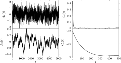
Figure 1: Two stochastic signals (left) and their respective connected time correlations (right). Correlation times are $\tau\approx 4.5$ (top), $\tau\approx 100$ (bottom). The signals were generated through Eq. (41) with $\mu=0$, $\sigma^{2}=2$, $N=10^{5}$, and $w=0.8$ (top), $w=0.99$ (bottom).

II.4 Correlations in Fourier space

Correlation functions are often studied in frequency space, either because they are obtained experimentally in the frequency domain (e.g. in techniques like dielectric spectroscopy), because the Fourier transforms are easier to compute or handle analytically, or because they provide an easier or alternative interpretation of the fluctuating process. Although the substance is the same, the precise definitions used can vary. One must pay attention to i) the convention used for the Fourier transform pairs and ii) the exact variables that are transformed.

Here we define the Fourier transform pairs as

$$\tilde{f}(\mathbf{k},\omega)=\int_{-\infty}^{\infty}\!\!dt\int\!\!d^{d}r\,f(\mathbf{r},t)e^{-i\mathbf{k}\cdot\mathbf{r}+i\omega t},\qquad f(\mathbf{r},t)=\int_{-\infty}^{\infty}\!\frac{d\omega}{2\pi}\int\!\!\frac{d^{d}r}{(2\pi)^{d}}\,\tilde{f}(\mathbf{k},\omega)e^{i\mathbf{k}\cdot\mathbf{r}-i\omega t},$$ (26)

but some authors choose the opposite sign for the forward transform and/or a different placement for the $1/2\pi$ factor (sometimes splitting it between the forward and inverse transforms). Depending on the convention a factor $2\pi$ can appear or disappear in some relations.

Let us consider time-only correlations first. These are defined in terms of two times, $t_{1}$ and $t_{2}$ (which we chose to write as $t_{0}$ and $t_{0}+t$). One can transform one or both of $t_{1}$ and $t_{2}$ or $t_{0}$ and $t$. Let us mention two different choices, useful in different circumstances. First, take the connected time correlation (10) and do a Fourier transform on $t$:

$$C_{c}(t_{0},\omega)=\int\!\!dt\,e^{i\omega t}C_{c}(t_{0},t_{0}+t)=e^{-i\omega t_{0}}\left\langle\delta A(t_{0})\delta\tilde{A}(\omega)\right\rangle,$$ (27)

where $\delta\tilde{A}(\omega)$ stands for the Fourier transform of $\delta A(t)$. This definition is convenient when there is an explicit dependence on $t_{0}$ but the evolution with $t_{0}$ is slow, as in the physical aging of glassy systems (see e.g. Cugliandolo, 2004); one then studies a time-dependent spectrum. If on the other hand $C_{c}$ is stationary, it is more convenient to write $t_{1}=t_{0}$, $t_{2}=t_{0}+t$ and do a double transform in $t_{1}$, $t_{2}$:

$$\tilde{C}_{c}(\omega_{1},\omega_{2})=\int\!\!dt_{1}\,dt_{2}\,e^{i\omega_{1}t_{1}}e^{i\omega_{2}t_{2}}C_{c}(t_{1},t_{2}-t_{1})=\\ \int\!\!dt_{1}\,dt_{2}\,e^{i\omega_{1}t_{1}}e^{i\omega_{2}t_{2}}\left\langle\delta A(t_{1})\delta A(t_{2})\right\rangle=\left\langle\delta\tilde{A}(\omega_{1})\delta\tilde{A}(\omega_{2})\right\rangle=\\ \int\!\!dt_{1}\,dt_{2}\,e^{i(\omega_{1}+\omega_{2})t_{1}}e^{i\omega_{2}(t_{2}-t_{1})}C_{c}(t_{2}-t_{1})=(2\pi)\delta(\omega_{1}+\omega_{2})\tilde{C}_{c}(\omega_{2}),$$ (28)

where $\tilde{C}_{c}(\omega)$ is the Fourier transform of the stationary connected correlation with respect to $t$ and we have used the integral representation of Dirac’s delta, $\delta(\omega-\omega^{\prime})=(2\pi)^{-1}\int_{-\infty}^{\infty}e^{it(\omega-\omega^{\prime})}\,dt$. As (28) shows, the transform is zero unless $\omega_{1}=-\omega_{2}$, so that it is useful to define the reduced correlation,

$$C_{c}^{R}(\omega)=\left\langle\delta\tilde{A}(-\omega)\delta\tilde{A}(\omega)\right\rangle=\left\langle\delta\tilde{A}^{*}(\omega)\delta\tilde{A}(\omega)\right\rangle,$$ (29)

where the rightmost equality holds when $A$ is real.

The transform $\tilde{C}_{c}(\omega)$ is a well-defined function, because the connected correlation decays to zero (and usually fast enough). We can then say

$$\tilde{C}_{c}(\omega)=\frac{1}{2\pi\delta(0)}C_{c}^{R}(\omega).$$ (30)

This relation can be exploited to build a very fast algorithm to compute $C_{c}(t)$ in practice (App. D). The at first sight baffling infinite factor relating the reduced correlation to $\tilde{C}_{c}(\omega)$ originates in the fact that $\delta\tilde{A}(\omega)$ cannot exist as an ordinary function, since we have assumed that $A(t)$ is stationary. This implies that the signal has an infinite duration, and that, its statistical properties being always the same, it cannot decay to zero for long times as required for its Fourier transform to exist. The Dirac delta can be understood as originating from a limiting process where one considers signals of duration $T$ (with suitable, usually periodic, boundary conditions) and then takes $T\to\infty$. Then $2\pi\delta(\omega=0)=\int\!\!dt\,e^{it\omega}|_{\omega=0}=\int\!\!dt=T$. These considerations can be made rigorous by defining the signal’s power spectrum,

$$h(\omega)=\lim_{T\to\infty}\frac{1}{T}\left\langle A_{T}(\omega)A_{T}^{*}(\omega)\right\rangle,\qquad A_{T}(\omega)=\int_{-T/2}^{T/2}A(t)e^{i\omega t}\,dt,$$ (31)

and then proving that $h(\omega)=\tilde{C}_{c}(\omega)$ (Priestley, 1981, §4.7, §4.8).

The same considerations apply to space or space-time correlations. For reference, the relations one finds are

$$\tilde{C}_{c}(\mathbf{k}_{1},\omega_{1},\mathbf{k}_{2},\omega_{2}) =\int\!\!d^{d}r_{1}\,dt_{1}\,d^{d}r_{2}\,dt_{2}\,e^{-i\mathbf{k}_{1}\cdot\mathbf{r}_{1}+i\omega_{1}t_{1}}e^{-i\mathbf{k}_{2}\cdot\mathbf{r}_{2}+i\omega_{2}t_{2}}C_{c}(\mathbf{r}_{1},t_{1},\mathbf{r}_{2}-\mathbf{r}_{1},t_{2}-t_{1}),$$ (32a)

$$\tilde{C}_{c}(\mathbf{k},\omega) =\int_{-\infty}^{\infty}\!\!dt\int\!\!d^{d}r\,e^{-i\mathbf{k}\cdot\mathbf{r}+i\omega t}C_{c}(\mathbf{r},t),$$ (32b)

$$C_{c}^{R}(\mathbf{k},\omega) =\left\langle\delta a(-\mathbf{k},-\omega)\delta a(\mathbf{k},\omega)\right\rangle,$$ (32c)

$$\tilde{C}_{c}(\mathbf{k}_{1},\omega_{1},\mathbf{k}_{2},\omega_{2}) =(2\pi)^{d+1}\delta^{(d)}(\mathbf{k}_{1}+\mathbf{k}_{2})\delta(\omega_{1}+\omega_{2})C_{c}^{R}(\mathbf{k}_{1},\omega_{1}),$$ (32d)

$$\tilde{C}_{c}(\mathbf{k},\omega) =\frac{1}{(2\pi)^{d+1}\delta^{(d)}(0)\delta(0)}C_{c}^{R}(\mathbf{k},\omega)=\frac{1}{(2\pi)^{d+1}VT}C_{c}^{R}(\mathbf{k},\omega).$$ (32e)

III Computing correlation functions from experimental data

The theoretical definitions of correlation functions are given as of averages over some probability distribution, or ensemble. To compute them in practice, given data recorded in an experiment or produced in numerical simulation, there are two issues two consider. First, experimental data will be discrete in time as well as in space, either as a result of sampling, or because the spatial resolution is high enough to measure the actual discrete units that make up our system (“particles”, i.e. birds, cells, neurons, etc.). Second, we do not have direct access to the probability distribution, but only to a set of samples, i.e. results from experiments, distributed randomly according to an unknown distribution. Thus we what we actually compute are estimators (as they are called in statistics) of the averages we want (the correlation functions). We will discuss estimators corresponding to different situations, and for clarity it will be convenient to consider first the case of a global quantity (correlation in time only, §III.1) and only later introduce the additional complications brought in by the space structure (§III.2).

Before moving to the estimation of correlations, let us examine the estimator for the mean, which we will need to estimate the connected correlation functions, and which will allow us to make a couple of general points. It is clearly hopeless to attempt to estimate an ensemble average unless it is possible to obtain many samples under the same conditions (i.e., if one is throwing dice, one should throw many times the same dice). So we assume that we are given a set of $M$ samples $\{a^{(n)}\}$, $n=1,\ldots,M$ obtained in $M$ equivalent experiments. From these samples we can estimate the mean as

$$\overline{a}=\frac{1}{M}\sum_{n=1}^{M}a^{(n)}.$$ (33)

This well-known estimator has the desirable property that it “gets better and better” when the number of samples $M$ grows, if the ensemble has finite variance. More precisely, $\overline{a}\to\left\langle a\right\rangle$ as $M\to\infty$. This property is called consistency, and is guaranteed because $\left\langle\overline{a}\right\rangle=\left\langle a\right\rangle$ (i.e. the estimator is unbiased) and the variance of $\overline{a}$ vanishes for $M\to\infty$ (Priestley, 1981, §5.2, §5.3).

How far off the estimate can be expected to be from the actual value (i.e. the “error”), is proportional to its variance. A result called the Cramer-Rao inequality implies that there is a lower bound to the variance of any estimator, given the number of samples (Priestley, 1981, §5.2). So in practice one of course chooses a good known estimator such as (33), but the only way to improve on the error is to acquire more samples, since the variance of (33) goes as $\sim 1/\sqrt{M}$. Unfortunately $1/\sqrt{M}$ is not a very fast-decreasing function (a tenfold increase in the number of samples reduces the error only by about a third), so one is always pressed to obtain the largest possible number of samples. But in experiments (especially in biology) the number of samples may be scarce, and more so in the case of correlations, which are defined in terms of pairs of values, separated by a fixed distance or time.

To make the most out of the available samples, one must take advantage of the known symmetries of the system. Space translation invariance, allows us to treat samples measured at different points of a large sample as different equivalent experiments, and the same goes for samples obtained at different points in time (even if the experiment has not been restarted) if the system is stationary. The samples obtained this way are in general not independent (they will be in fact correlated), but the estimate (33) does not need to be used on independent samples. It is still unbiased and consistent, only that its variance will be larger than it would be for the same number of independent samples (see Eq. (38)).

Accordingly, whenever in what follows we use $n$ to index samples or experiments, it is understood that the averages over $n$ can actually be implemented as averages over a time or space index if the system is stationary or homogeneous, respectively. We refer then to time averages or space averages as replacing ensemble averages when building an estimator.

III.1 Estimation of time correlation functions

Assume that the experiment records a scalar signal with a uniform sampling interval $\Delta t$, so that we are handled $N$ real-valued and time-ordered values forming a sequence $A_{i}$, with $i=1,\ldots,N$. It is understood that if the data are digitally sampled from a continuous time process, proper filtering has been applied. In what follows we shall measure time in units of the sampling interval, so that in the formulae below we shall make no use of $\Delta t$. To recover the original time units one must simply remember that $A_{i}=A(t_{i})$ with $t_{i}=t_{0}+(i-1)\Delta t$. For the stationary case we shall write $C_{k}=C(t_{k})$ where $t_{k}$ is the time difference, $t_{k}=k\Delta t$ and $k=0,\ldots,N-1$, and in the non-stationary case $C_{i,k}=C(t_{i},t_{k})$.

If the process is not stationary, nothing can be estimated from a single sequence because the successive values correspond to different, nonequivalent experiments, as the conditions have changed from one sample to another (i.e. the system has evolved in a way that has altered the characteristic of the stochastic process). In this case the correlation depends on two times and the mean itself can depend on time. The only way to estimate the mean or the correlation function is to obtain many sequences $A_{i}^{(n)}$, $n=1,\ldots,M$ reinitializing the system to the same macroscopic conditions each time (in a simulation, one can for example restart the simulation with the same parameters but changing the random number seed). It is not possible to resort to time averaging, and the estimates are obtained by replacing the ensemble average by averages across the different sequences, i.e. the (time-dependent) mean is estimated as

$$\left\langle A(t_{i})\right\rangle\approx\overline{A_{i}}=\frac{1}{M}\sum_{n=1}^{M}A_{i}^{(n)},$$ (34)

and the time correlation as

$$C_{c}(t_{i},t_{k})\approx\hat{C}^{(c)}_{i,k}=\frac{1}{M}\sum_{n}^{M}\delta A_{i}^{(n)}\delta A_{i+k}^{(n)},\qquad\delta A_{i}^{(n)}=A_{i}^{(n)}-\overline{A_{i}},$$ (35)

where the hat distinguishes the estimate from the actual quantity. Both estimators are consistent and unbiased, i.e. $\hat{C}^{(c)}_{i,k}\to C(t_{i},t_{i})$ and $\overline{A(t_{i})}\to\left\langle A(t_{i})\right\rangle$ for $M\to\infty$.

If the system is stationary, one can resort to time averaging to build estimators (like (37) below) that only require one sequence. But let us remark that it is always sensible to check whether the sequence is actually stationary. A first check on the mean can be done dividing the sequence in several sections and computing the average of each section, then looking for a possible systematic trend. If this check passes, then one should compute the time correlation of each section and then checking that all of them show the same decay (using fewer sections than in the first check, as longer sections will be needed to obtain meaningful estimates of the correlation function). It is important to note that this second check is necessary even if the first one passes; as we it is possible for the mean to be time-independent (or its time-dependence undetectable) while the time correlation still depends on two times.

In the stationary case, then, we can estimate the mean with

$$\overline{A}=\frac{1}{N}\sum_{i=1}^{N}A_{i},$$ (36)

and the connected correlation function with

$$\hat{C}^{(c)}_{k}=\frac{1}{N-k}\sum_{j=1}^{N-k}\delta A_{j}\delta A_{j+k},\qquad\delta A_{j}=A_{j}-\overline{A}.$$ (37)

In the last equation, the true sample mean $\left\langle A\right\rangle$, if known, can be used instead of the estimate $\overline{A}$. If the true mean is used, the estimator (37) is unbiased, otherwise it is asymptotically unbiased, i.e. the bias tends to zero for $N\to\infty$, provided the Fourier transform of $C_{c}(t)$ exists. More precisely, $\langle\hat{C}^{(c)}_{k}\rangle=C_{c}(t_{k})-\alpha/N$, where $\alpha=2\pi\text{Var}_{A}\tilde{C}_{c}(\omega=0)$. The variance of $\hat{C}^{(c)}_{k}$ is $O(\frac{1}{N-k})$ (Priestley, 1981, §5.3). This is sufficient to show that, at fixed $k$, the estimator is consistent, i.e. $\hat{C}^{(c)}_{k}\to C_{c}(t_{k})$ for $N\to\infty$. However, the variance grows with increasing $k$, and thus the tail of $\hat{C}^{(c)}_{k}$ is considerably noisy. In practice, for $k$ near $N$ the estimate is mostly useless, and the usual rule of thumb is to use $\hat{C}^{(c)}_{k}$ only for $k\leq N/2$.

Knowing the time correlation, one can make the statement that the variance of the estimate (36) is larger than that of (34) quantitative: the variance of the estimate with correlated samples is Sokal (1997)

$$\text{Var}_{\overline{a}}\approx\frac{2\tau_{\text{int}}}{N}\left[\left\langle A^{2}\right\rangle-\left\langle A\right\rangle^{2}\right],$$ (38)

i.e. $2\tau_{\text{int}}$ times larger than the variance in the independent sample case, where $\tau_{\text{int}}$ is the integral correlation time defined below (58). In this sense $N/2\tau_{\text{int}}$ can be thought of as the number of “effectively independent” samples.

We have not written an estimator for the nonconnected correlation function. It is natural to propose

$$\hat{C}_{k}=\frac{1}{N-k}\sum_{j=1}^{N-k}A_{j}A_{j+k}.$$ (39)

However, although $\hat{C}_{k}$ is unbiased, it can have a large variance when the signal has a mean value larger than the typical fluctuation (see §III.1.1). As a general rule, it is not a good idea estimate the connected correlation by using (39) and then subtracting $\overline{A}^{2}$. Instead, the connected estimator (37) should be used. An possible exception may be the case when an experiment can only furnish many short independent samples of the signal (see the examples in §III.1.2).

If several sequences sampled from a stationary system are available, it is possible to combine the two averages: one first computes the stationary correlation estimate (37) for each sequence, and then averages the different correlation estimates (over $n$ at fixed lag $k$). It is clearly wrong to average the sequences themselves before computing the correlation, as this will tend to approach the (stationary) ensemble mean $\left\langle A\right\rangle$ for all times, destroying the dynamical correlations.

There is another asymptotically unbiased estimator of the connected correlation, that can be obtained by using $1/N$ instead of $1/(N-i)$ as prefactor of the sum in (37). Calling this estimator $C_{c,k}^{*}$, it holds that $\langle C_{c,k}^{*}\rangle=C_{c}(t_{k})-\alpha/N-kC(t_{k})/N-\alpha k/N^{2}$, where $\alpha$ is defined as before, and again $\alpha=0$ if the exact sample mean is used (Priestley, 1981, §5.3). This has the unpleasant property that the bias depends on $k$, while the bias of $\hat{C}_{c,k}$ is independent of its argument, and smaller in magnitude. The advantage of $C_{c,k}^{*}$ is that its variance is $O(1/N)$ independent of $k$, thus it has a less noisy tail. Some authors prefer $C_{c,k}^{*}$ due to its smaller variance and to the fact that it strictly preserves properties of the correlation, which may not hold exactly for $\hat{C}_{c,k}$. Here we stick to $\hat{C}_{c,k}$, as usual in the physics literature (e.g. Sokal, 1997; Allen and Tildesley, 1987; Newman and Barkema, 1999), so that we avoid worrying about possible distortions of the shape. In practice however, it seems that as long as $N$ is greater than $\sim 10\tau$ (a necessary requirement in any case, see below), and for $k\leq N/2$, there is little numerical difference between the two estimates.

III.1.1 Two properties of the estimator

We must mention two important features of the estimator that are highly relevant when attempting to compute numerically the time correlation. The first is that the difference between the non-connected and connected estimators is not ${\overline{a}}^{2}$, but

$$\hat{C}_{k}-\hat{C}_{c,k}=\overline{a}\left[\frac{1}{N-k}\sum_{j}^{N-k}a_{j}+\frac{1}{N-k}\sum_{j}^{N-k}a_{j+k}-\overline{a}\right],$$ (40)

as it is not difficult to compute. The difference does tend to $\overline{a}^{2}$ for $N\to\infty$, but in a finite sample fluctuations are important, especially at large $k$. Since fluctuations are amplified by a factor $\overline{a}$, when the signal mean is large with respect to its variance, the estimate $\hat{C}_{k}$ is completely washed out by statistical fluctuations. This is why, while $C(t)$ and $C_{c}(t)$ differ by a constant, in practice it is a bad idea to compute $\hat{C}_{k}$ and subtract $\overline{a}^{2}$ to obtain an estimate of the connected correlation. Instead, one computes the connected correlation directly by estimating first the mean and then using (37).

Another important fact is that the estimator of the connected correlation will always have zero, whatever the length of the sample used, even if $N$ is much shorter than the correlation time. As shown in App. B, for any time series one has that $\hat{C}^{(c)}_{0}>0$ and that $\hat{C}^{(c)}_{c,k}$ will change sign at least once for $k\geq 1$ (this applies to the case when the mean and connected correlation are estimated with a single time series). The practical consequence is that when $N$ is of the order of $\tau$, or smaller, the estimate $\hat{C}^{(c)}_{k}$ will suffer from strong finite-size effects, and its shape will be quite different from the actual $C_{c}(t)$. In particular, since $\hat{C}^{(c)}_{k}$ will intersect the $x$-axis, it will look like the series has decorrelated when in fact it is still highly correlated. Be suspicious if $\hat{C}^{(c)}_{k}$ changes sign once and stays very anticorrelated. Anticorrelation may be a feature of the actual $C_{c}(t)$, but if the sample is long enough, the estimate should decay until correlation is lost (noisily oscillating around zero). One must always perform tests estimating the correlation with different values of $N$: if the shape of the correlation at short times depends on $N$, then $N$ must be increased until one finds that estimates for different values of $N$ coincide for lags up to a few times the correlation time (we show an example next). Once a sample-size-independent estimate has been obtained, the correlation time can be estimated (§IV.1), and it must be checked that self-consistently $N$ is several times larger than $\tau$.

III.1.2 Example

To illustrate the above considerations on estimating $C_{c}(t)$ we use a synthetic correlated sequence generated from the recursion

$$a_{i}=wa_{i-1}+(1-w)\xi_{i},$$ (41)

where $w\in[0,1]$ is a parameter and the $\xi_{i}$ are uncorrelated Gaussian random variables with mean $\mu$ and variance $\sigma^{2}$. Assuming the stationary state has been reached it is not difficult to find

$$\left\langle a\right\rangle=\mu,\qquad\left\langle(a-\mu)^{2}\right\rangle=\frac{1-w}{1+w}\sigma^{2},\qquad C^{(c)}_{k}=\left\langle(a_{i}-\mu)(a_{i+k}-\mu)\right\rangle=\sigma^{2}w^{k},$$ (42)

so that the correlation time is $\tau=-1/\log w$.

We used the above recursion to generate artificial sequences and computed their time correlation functions with the estimates discussed above. Fig. 2 shows the problem that can face the non-connected estimate. When the average of the signal is smaller than or of the order of the noise amplitude (as in the top panels), one can get away with using (39). However if $\mu\gg\sigma$, the non-connected estimate is swamped by noise, while the connected estimate is essentially unaffected (bottom panels). Hence, if one is considering only one sequence, one should always use the connected estimator.

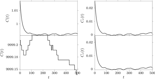
Figure 2: Connected vs. nonconnected estimate. The estimate of $C(t)$ (equation (39), left panels) is much worse that the estimates of $C_{c}(t)$ (equation (37), right panels). The (artificial) signal was generated with (41). Top panels: $\mu=1$; bottom panels: $\mu=100$. In both cases, $\sigma^{2}=1$, $w=0.95$ ($\tau\approx 20$) and length $N=5\cdot 10^{4}$.

In Fig. 3 we see how using samples that are too short affects the correlation estimates. The same artificial signal was generated with different lengths. For the shorter lengths, it is seen that the correlation estimate crosses the $t$ axis (as we have shown it must) but does not show signs of losing correlation. One might hope that $N=1000\approx 10\tau$ is enough (the estimate starts to show a flat tail), but comparing to the result of doubling the length shows that it is still suffering from finite-length effects. For this particular sequence, it is seen that at least $20\tau$ to $50\tau$ is needed to get the initial part of the normalized connected correlation more or less right, while a length of about 1000$\,\tau$ is necessary to obtain a good estimate up to $t\sim 5\tau$. The unnormalized estimator suffers still more from finite size due to the increased error in the determination of the variance (left panel).

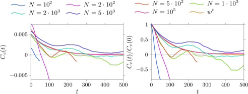
Figure 3: Finite size effects. Estimates of the connected correlation (left) and normalized connected correlation (right) for sequence (41) of different lengths as indicated, together with the analytical result $C_{c}(t)=\sigma^{2}w^{t}$. Parameters are $\mu=0$, $\sigma^{2}=1$, $w=0.99$ ($\tau\approx 100$).

If the experimental situation is such that it is impossible to obtain sequences much longer than the correlation time, one can get some information on the time correlation if it is possible to repeat the experiment so as to obtain several independent and statistically equivalent sample sequences. In Fig. 4 we take several sequences with the same parameters as in the previous example, but quite short ($N=200\approx 2\tau$). As we have shown, it is not possible to obtain a moderately reasonable estimate of $C_{c}(t)$ using one such sequence (as is also clear from the $M=1$ case of Fig. 4). However, the figure shows how one may benefit from the multiple repetitions of the (short) experiment by averaging together all the estimates. The averaged connected estimates are always far from the actual correlation function, even for $M=500$ (the case which contains in total $10^{5}$ points, which proved quite satisfactory in the previous example): this is consequence of the fact that all connected estimates must become negative. Instead, the averaged non-connected estimates approach quite closely the analytical result even though not reaching the decorrelated region. Although it is tricky to try to extract a correlation time from this estimate (due to lack of information on the last part of the decay), this procedure at least offers a way to obtain some dynamical information in the face of experimental limitations.

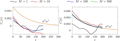
Figure 4: Effect of averaging the estimates of many short sequences. We show the connected (left) and non-connected (right) estimates of $M$ different samples of sequence (41) as indicated in the legend, with $N=200$, $\mu=0$, $\sigma^{2}=1$, $w=0.99$ ($\tau\approx 100$). The analytical result $C_{c}(t)=\sigma^{2}w^{t}$ is also plotted.

III.2 Estimation of space correlation functions

To compute space correlations one needs experimental data with spatial resolution. We can assume that each experiment provides us a set of values $\{a_{i}^{(n)}\}$ together with a set of positions $\{\mathbf{r}_{i}^{(n)}\}$ which specify where in the sample the $i$-th value has been recorded. The experiment label, $n=1,\ldots,M$ can indicate experiments on different samples, or for a stationary system, it can be a time index.

The positions $\mathbf{r}_{i}^{(n)}$ may be fixed by the experiment (e.g. when sampling in space with an array of sensors, in which case they are likely independent of $n$) or might be themselves part of the experimental result (as when measuring the positions of moving organisms). In the former case, a naive implementation of definition (12) will pick up the structure of the experimental array itself, introducing correlations that are clearly an artefact. In the latter case, the positions may encode nontrivial structural features, which will show up in the correlation function of $a$ together with $a$-specific effects. For example, particles with excluded volume will have non-trivial density correlations at short range, while there might be long-range correlations due to an ordering of $a$. It is then wise to untangle the two effects as much as possible. In both cases it is thus convenient to implement the definition in a way that separates structural correlations.

Structural effects can be studied through density correlation functions. One such function is the pair distribution function (Hansen and McDonald, 2005, §2.5), defined for homogeneous systems as

$$g(\mathbf{r})=\frac{1}{\rho_{0}N}\left\langle\sum_{i\neq j|}\delta^{(d)}(\mathbf{r}-\mathbf{r}_{ij})\right\rangle=\frac{1}{N\rho_{0}}\left\langle\sum_{i\neq j}\frac{\delta\bigl{(}\lvert\mathbf{r}\rvert-\lvert r_{ij}\rvert\bigr{)}}{4\pi\lvert\mathbf{r}\rvert^{2}}\right\rangle,$$ (43)

where $\delta^{(d)}(\mathbf{r})$ is the $d$-dimensional Dirac’s delta, $\mathbf{r}_{ij}=\mathbf{r}_{i}-\mathbf{r}_{j}$ is the pair displacement and $\rho_{0}=N/V$ is the average density. The second equality is valid for isotropic systems, and $g(r)$ is often called radial distribution function in this case. Defining the density of the configuration $\{\mathbf{r}_{i}\}$ by $\rho(\mathbf{r})=\sum_{i}\delta(\mathbf{r}-\mathbf{r}_{i})$, the pair distribution function is found to be related to the density-density correlation function by

$$\left\langle\rho(\mathbf{r}_{0})\rho(\mathbf{r}_{0}+\mathbf{r})\right\rangle=\rho_{0}^{2}g(\mathbf{r})+\rho_{0}\delta(\mathbf{r})=\rho_{0}^{2}g(\lvert\mathbf{r}\rvert)+\rho_{0}\frac{\delta(\lvert\mathbf{r}\rvert)}{4\pi\lvert\mathbf{r}\rvert^{2}},$$ (44)

where again the second equality applies to isotropic systems. The Dirac delta term arises because in $\left\langle\rho(\mathbf{r}_{0})\rho(\mathbf{r}_{0}+\mathbf{r})\right\rangle$ one includes the $i=j$ terms that were excluded from the sum in (43). If the $\{\mathbf{r}_{i}\}$ are obtained with periodic boundary conditions (as is often the case in simulation), (43) can be used to estimate $g(r)$ almost directly: it suffices to replace Dirac’s delta by a discrete version (i.e. turn it into a binning function) and the average by a (normalised) sum over all available statistically equivalent configurations. For the isotropic case,

$$\hat{g}_{k} =\frac{1}{M}\sum_{n}\frac{1}{\rho_{0}N}\sum_{ij}\frac{\Delta\left[r_{ij}^{(n)}-(k+1/2)\Delta r\right]}{V_{k}},$$ (45a)

$$\Delta(r) =\begin{cases}1&\text{if }-\Delta r/2<r\leq\Delta r/2,\\ 0&\text{otherwise}.\end{cases}$$ (45b)

where $\Delta r$ is the bin width and $V_{k}$ is the volume of the $k$-th bin, in 3 dimensions $V_{k}=\frac{4}{3}\pi(\Delta r)^{3}\left((k+1)^{3}-k^{3}\right)$. The bin width must not be chosen too small or some bins will end up having very few or no particles. In any case, it must be larger than the experimental resolution, otherwise $g(r)$ will pick up spurious correlations arising from the fact that due to finite spatial resolution, all positions effectively lay on the sites of a square lattice.

If borders are non-periodic, as in experimental data, using (49) will introduce bias at large $r$, because the number of neighbours of a given particle stops growing as $r^{2}$ (the volume of the bin) as soon as $r$ is of the order of the distance of the particle to the nearest border. In this case an unbiased estimator is

$$\hat{g}_{k} =\frac{1}{\rho_{0}N_{k}}\sum_{i\in S_{k}}\sum_{j}\frac{\Delta(k-r_{ij}/\Delta r)}{V_{k}},$$ (46)

where $i\in S_{k}$ means that the sum runs only over the set of particles that are at least at a distance $(k+1/2)\Delta r$ from the nearest border, and $N_{k}$ is the number of such particles. In other words, for a given point $i$, the pair $ij$ only enters the sum if $\mathbf{r}_{j}$ lies on a bin (centred at $i$) that is completely contained within the system’s volume. This is known as the unweighted Hanisch method (Hanisch, 1984).

To conclude our remarks on structural correlation functions, let us note that if correlations in Fourier space are of interest, it is typically better to estimate them directly, rather than going through the real space functions and applying a numerical Fourier transform. For example, the structure factor, which is proportional to the reduced density correlation,

$$S(\mathbf{k})=\frac{1}{N}\left\langle\rho(\mathbf{k})\rho(-\mathbf{k})\right\rangle=1+\rho_{0}\tilde{g}(\mathbf{k}),$$ (47)

where $\tilde{g}(\mathbf{k})$ is the Fourier transform of $g(\mathbf{r})$, can be be computed directly from the $\mathbf{r}_{i}^{(n)}$ through

$$S(\mathbf{k})=\frac{1}{M}\frac{1}{N}\sum_{n}\sum_{jl}e^{i\mathbf{k}\cdot\mathbf{r}_{jl}^{(n)}}=1+\frac{1}{NM}\sum_{n}\sum_{i\neq j}\frac{\sin\lvert\mathbf{k}\rvert r_{ij}^{(n)}}{\lvert\mathbf{k}\rvert r_{ij}^{(n)}},$$ (48)

where again the second equality applies to isotropic system and is obtained by analytically averaging the first expression over all angles. For further discussion of density correlation functions we refer the reader to condensed matter texts such as Hansen and McDonald (2005) or Ashcroft and Mermin (1976).

Turning now to the correlations of $a$, and focusing on the homogeneous case, we seek an estimator of the connected correlation function. How to write it depends on exactly what one means by $a(\mathbf{r})$ (it can be defined as a density or as specific quantity, i.e. per unit volume or per particle), and on the fact that one wants to separate structural correlations. These issues are discussed at length in Cavagna et al. (2018). Here it will suffice to state that a good estimator is

$$\hat{C}^{(c)}(\mathbf{r})=\frac{\sum_{ij}\delta a_{i}\delta a_{j}\delta(\mathbf{r}-\mathbf{r}_{ij})}{\sum_{kl}\delta(\mathbf{r}-\mathbf{r}_{kl})}=\frac{\sum_{ij}\delta a_{i}\delta a_{j}\delta(r-r_{ij})}{\sum_{kl}\delta(r-r_{kl})},$$ (49)

where again $\delta a_{i}=a_{i}-\overline{a}$ and the last expression is for the isotropic case. We have written $\delta$ functions for clarity, but clearly one uses binning as in (45). These expressions do a good job of disentangling correlations of the property $a$ from structural correlations. In the case of a fixed lattice, $\hat{C}^{(c)}(\mathbf{r})$ is completely emancipated from the effects of the lattice structure, while in the case of moving particles, at least the uncorrelated effects of structure will be taken care of. Also, thanks to the denominator, (49) is free from boundary effects, so that one does need to worry about the border bias that requires the use of the Hanisch method for $g(r)$.

As written, (49) can be computed using a single configuration. Since the system is homogeneous, the mean $\left\langle a\right\rangle$ can also be estimated with a space average,

$$\overline{a}=\frac{1}{N}\sum_{i}a_{i}.$$ (50)

We shall write $\hat{C}^{(c)}_{\text{sp}}(r)$ (for space average) when it is computed for single configurations. If several configurations equivalent and with the same boundary conditions, are available, additional averaging using these can be performed. We shall still call the estimate a space average if the correlation is first computed for each configurations, with the mean estimated with a average of the same configuration, and the average over configurations is done afterwards.

Another way to proceed is to use all configurations to compute first an estimate of the mean, and then compute the correlation. In this case we shall write $\hat{C}^{(c)}_{\text{ph}}(r)$, for phase average, because this procedure is closest to actually performing a phase-space, or ensemble, average.

An important fact about the estimate  (49) in the space-average case is that $\hat{C}^{(c)}_{\text{sp}}(\mathbf{r})$ will always have a zero, exactly like the estimator for the connected time correlation (37). The reason is similar, and it can be seen considering that since $\sum_{i}\delta a_{i}=0$, then

$$0=\frac{1}{N}\sum_{ij}\delta a_{i}\delta a_{j}=\rho_{0}\int\!\!d\mathbf{r}\,g_{F}(\mathbf{r})C(\mathbf{r}),$$ (51)

where $g_{F}(\mathbf{r})$ is defined as the pair distribution function (43) but without excluding the case $i=j$ from the double sum. Since $g_{F}(r)>0$, it follows that $\hat{C}^{(c)}_{\text{sp}}(\mathbf{r})$ must change sign, so there is always an $r_{0}$ such that $\hat{C}^{(c)}_{\text{sp}}(r_{0})=0$. This is an artefact, but it can be exploited to obtain a proxy of the correlation scale in critical systems (§V.2).

Let us conclude by writing the Fourier-space counterpart of $\hat{C}^{(c)}(r)$. We introduce it as proportional to the reduced correlation,

$$\hat{C}(\mathbf{k})=\frac{1}{N}\delta a(\mathbf{k})\delta(-\mathbf{k})=\frac{1}{N}\sum_{ij}\delta a_{i}\delta a_{j}e^{i\mathbf{k}\cdot\mathbf{r}_{ij}}=\frac{1}{N}\sum_{ij}\frac{\sin\lvert\mathbf{k}\rvert r_{ij}}{\lvert\mathbf{k}\rvert r_{ij}}\delta a_{i}\delta a_{j}.$$ (52)

It is related to the real space correlation by

$$\hat{C}(k)=\rho_{0}\int\!\!d\mathbf{r}\,g_{F}(r)e^{-i\mathbf{k}\cdot\mathbf{r}}\hat{C}^{(c)}(r).$$ (53)

The function $g_{F}(r)$ appears in the integral (in effect reintroducing structural effects in $\hat{C}(k)$) because (52) is more convenient computational-wise than the Fourier transform of (49), and is consistent with an integration measure chosen so that the integral of $a(r)$ equals $\sum_{i}a_{i}$, which is often the global order parameter (see Cavagna et al., 2018, App. A).

III.3 Estimation of space-time correlations

Space-time correlation estimation brings together the issues encountered in the time and space cases. The previous discussion should allow the reader to generalise the estimators written above to the space-time case. For brevity, let us just write the space-time generalisation of (49) and  (52) (for homogeneous and stationary systems):

$$\hat{C}^{(c)}(\mathbf{r},t) =\frac{1}{T}\sum_{t_{0}}\frac{\sum_{ij}\delta a_{i}(t_{0})\delta a_{j}(t_{0}+t)\delta(\mathbf{r}-\mathbf{r}_{i}(t_{0})+\mathbf{r}_{j}(t_{0}+t))}{\sum_{ij}\delta(\mathbf{r}-\mathbf{r}_{i}(t_{0})+\mathbf{r}_{j}(t_{0}+t))},$$ (54)

$$\hat{C}(\mathbf{k}) =\frac{1}{TN}\sum_{t_{0}}\sum_{ij}\delta a_{i}(t_{0})\delta a_{j}(t_{0}+t)e^{-i\mathbf{k}\cdot[\mathbf{r}_{i}(t_{0})-\mathbf{r}_{j}(t_{0}+t)}.$$ (55)

IV Correlation length and correlation time

A connected space correlation function measures how correlation is gradually lost as one considers two locations further and further apart. Similarly, the connected time correlation function measures how correlation is gradually lost as time elapses. One often seeks for a summary of this detailed information, in the form of a (space or time) scale that measures the interval it takes for significant decorrelation to happen: these are the correlation length $\xi$ and the correlation time $\tau$.

Sometimes these are interpreted as the distance or time after which the connected correlation has descended past a prescribed level. Although this can be a useful operational definition when working with a set of correlation functions of similar shape, these scales are better understood as the asymptotic exponential rate of the decay. The precise numerical value (which will depend on the details of the computation method) is less important than their trend with the relevant control parameters (temperature, concentration, $\ldots$): in this sense one can say that $\xi$ and $\tau$ are most useful to compare the correlation range as some environmental condition is changed.

Of course, correlation functions are typically more complicated than a simple exponential, and it may make sense to describe them using more than one scale (e.g. as a superposition of exponential decays). The correlation length refers to the rate of the last exponential to die out. More precisely (Amit and Martín-Mayor, 2006, §II.2-3)

$$\xi=\lim_{r\to\infty}\frac{r}{-\log C_{c}(r)}.$$ (56)

This definition, with emphasis on the long-range behaviour, is particularly suited to the study of systems in the critical region. Note that $\xi=\infty$ does not mean that the correlation never decays, but only that it does so slower than exponentially (i.e. as a power law).

Similarly, the correlation time is (Sokal, 1997),

$$\tau=\lim_{t\to\infty}\frac{t}{-\log C_{c}(t)}.$$ (57)

These definitions work well when the decay is a combination of exponentials and power laws. Exponentials of powers, on the other hand, never yield a finite scale according to (56) or (57), we defer discussion of those to App. C.

Clearly definitions (56) and (57) are not directly applicable to extract $\xi$ or $\tau$ from correlation functions computed in experiments or simulations, which are of finite range. The rest of this section is devoted to discussing ways to obtain $\xi$ or $\tau$ from finite data.

A possibility is to fit the decay to some function, and apply the definitions to this function. This may be fine, as long as one can avoid proliferation of parameters. However, it can be difficult to fit both the short- and long-range regimes, so an alternative is to attempt fit $\log\left[x^{\alpha}C_{c}(x)\right]$ (where $x$ stands for $r$ or $t$) for large $x$ with straight line $-Ax$. If the fit is good then one has $\xi=1/A$ or $\tau=1/A$. One expects $\alpha=0$ for the time case (at least in equilibrium), and in the space case $\alpha\approx 0$ in $d=2$ and $\alpha\approx 1$ in $d=3$ according to the scaling form (66). This power has no effect on the definition (56), but is important to obtain a reasonable fit on relatively short range.

Nevertheless, fitting may not be the best strategy, especially if the linear region in the fit is short and the slope is very sensitive to the choice of fitting interval. We present next some alternative procedures.

IV.1 Correlation time

A quite general way to define a correlation time is from the integral of the normalized connected correlation,

$$\tau_{\text{int}}=\int_{0}^{\infty}\rho(t)\,dt.$$ (58)

Clearly for a pure exponential decay $\tau_{\text{int}}=\tau$. In general, if $\rho(t)=f(t/\tau)$ then $\tau_{\text{int}}=\text{const}\,\tau$, so that $\tau_{\text{int}}$ has the same dependence on control parameters as $\tau$. This would change if $\rho(t)=(t/t_{0})^{\alpha}f(t/\tau)$ (Sokal, 1997, §2), but one expects $\alpha=0$ in equilibrium. In any case, $\tau_{\text{int}}$ has a meaning of its own, as the scale that corrects the variance of the estimate of the mean when computed with correlated samples (§III.1).

With some care, $\tau_{\text{int}}$ can be computed from experimental or simulation data, avoiding the difficulties associated with thresholds or fitting functions. The following procedure Sokal (1997) is expected to work well if long enough sequences are at disposal and the decay does not display strong oscillations or anticorrelation. If $\hat{C}^{(c)}_{k}\approx C_{c}(k\Delta t)$ is the estimate of the stationary connected correlation (37), then the integral can be approximated by a discrete sum. However, the sum cannot run over all available values $k=0,\ldots,N-1$, because the variance of $\hat{C}^{(c)}_{k}$ for $k$ near $N-1$ is large (§III.1), so that the sum $\sum_{k=0}^{N-1}\hat{C}^{(c)}_{k}$ is dominated by statistical noise (more precisely, its variance does not go to zero for $N\to\infty$). A way around this difficulty is (Sokal, 1997, §3) to cut-off the integral at a time $t_{c}=c\Delta t$ such that $c\ll N$ but the correlation is already small at $t=t_{c}$ (i.e. $t_{c}$ is a few times $\tau$). Thus $\tau_{\text{int}}$ is defined self-consistently as

$$\tau_{\text{int}}=\int_{0}^{\alpha\tau_{\text{int}}}\rho(t)\,dt,$$ (59)

where $\alpha$ should be chosen larger than about $5$, and within a region of values such that $\tau_{\text{int}}(\alpha)$ is approximately independent of $\alpha$. Longer tails will require larger values of $\alpha$; we have found adequate values to be as large as 20 (Cavagna et al., 2012). To solve (59) one can compute $\tau(M)=\sum_{k}^{M}\hat{C}^{(c)}_{k}/\hat{C}^{(c)}_{0}$ starting with $M=1$ and increasing $M$ until $\alpha\tau(M)>M$.

Another useful definition of correlation time can be obtained from $\tilde{\rho}(\omega)$, the Fourier transform of $\rho(t)$. Normalisation of $\rho(t)$ implies that $1=\rho(0)=\int_{-\infty}^{\infty}\frac{d\omega}{2\pi}\,\tilde{\rho}(\omega)$. Then a characteristic frequency $\omega_{0}$ (and a characteristic time $\tau_{0}=1/\omega_{0}$) can be defined such that half of the spectrum of $\tilde{\rho}(\omega)$ is contained in $\omega\in[-\omega_{0},\omega_{0}]$ Halperin and Hohenberg (1969), i.e.

$$\int_{-\omega_{0}}^{\omega_{0}}\frac{d\omega}{2\pi}\,\tilde{\rho}(\omega)=\frac{1}{2}.$$ (60)

This definition of can be expressed directly in the time domain writing

$$\frac{1}{2}=\int_{-\omega_{0}}^{\omega_{0}}\frac{d\omega}{2\pi}\int_{-\infty}^{\infty}\!\!dt\,\rho(t)e^{i\omega t}=2\int_{0}^{\infty}\!\!dt\rho(t)\int_{-\omega_{0}}^{\omega_{0}}\frac{d\omega}{2\pi}e^{i\omega t}=\frac{2}{\pi}\int_{0}^{\infty}\!\!dt\,\rho(t)\frac{\sin\omega_{0}t}{t},$$ (61)

where we have used the fact that $\rho(t)$ is even. Then the correlation time is defined by

$$\int_{0}^{\infty}\!\!\frac{dt}{t}\,\rho(t)\sin\left(\frac{t}{\tau_{0}}\right)=\frac{\pi}{4}.$$ (62)

It can be seen that if $\rho(t)=f(t/\tau)$, then $\tau_{0}$ is proportional to $\tau$ (it suffices to change the integration variable to $u=t/\tau$ in the integral above). An advantage of this definition is that it copes well with the case when inertial effects are important and manifest in (damped) oscillations of the correlation function (see Fig. 10).

IV.2 Correlation length

A quite general procedure is to use the second moment correlation length $\xi_{2}$ (Amit and Martín-Mayor, 2006, §2.3.1),

$$\xi_{2}=\sqrt{\frac{\int\!\!d\mathbf{r}\,r^{2}C_{c}(\mathbf{r})}{\int\!\!d\mathbf{r}\,C_{c}(\mathbf{r})}}.$$ (63)

The quotient here ensures that $\xi_{2}$ scales with control parameters like $\xi$ (a definition analogous to that of the integral correlation time would not have this property due to the power-law prefactor). $\xi_{2}$ can also be expressed in terms of the Fourier transform of $C_{c}(\mathbf{r})$ as

$$\xi_{2}^{2}=-\left.\frac{1}{\tilde{C}(\mathbf{k})}\frac{\partial^{2}\tilde{C}(\mathbf{k})}{\partial k_{\alpha}\partial k_{\alpha}}\right\rvert_{k=0}.$$ (64)

The integrals in (63) can be computed numerically over the finite volume, but (64) may be more convenient (recall that $\hat{C}(\mathbf{k})$ can be computed directly from the data, §III.2). Numerical derivatives should clearly be avoided; instead one can fit $\tilde{C}(k)^{-1}=A+Bk^{2}$ for small $k$, and obtain the correlation length as $\xi_{2}=\sqrt{B/A}$ (which follows from (64) apart from a dimensional-dependent numerical prefactor). Another possibility is to obtain $A$ and $B$ using only $\tilde{C}(0)$ and $\tilde{C}(k_{\text{min}})$ (Cooper et al., 1982), where $k_{\text{min}}$ is the smallest wavenumber allowed by boundary conditions (e.g. $k_{\text{min}}=2\pi/L$ in a cubic periodic system), resulting in

$$\xi_{2}=\frac{1}{k_{\text{min}}}\sqrt{\frac{\hat{C}(0)}{\hat{C}(k_{\text{min}})}-1}.$$ (65)

When working with lattice systems, $2\sin(k_{\text{min}}/2)$ can be substituted for the $k_{\text{min}}$ outside the square root (Caracciolo et al., 1993), rendering the expression exact for a Gaussian lattice model. This procedure works well when $\xi\ll L$, so that the small wavevectors are seeing an exponential behaviour for $r\sim L$.

If $A/B$ is not much larger than $L^{-2}$, then $\xi$ is approaching the system size $L$ and the estimate is not very reliable; for $\xi$ of the order of $L$ or larger, $A/B$ may even become negative. In situations like these (which include critical systems), the first root of $\hat{C}^{(c)}_{\text{sp}}(r)$, can provide a useful proxy for the correlation scale, but it is necessary to compare systems of different sizes (see §V.2).

V Correlation functions in the critical region

The critical region refers to the volume of parameter space near the critical surface, which is a boundary between different phases of a system. The word phase may refer to a thermodynamic equilibrium phase, but it also applies to systems out of equilibrium, where different phases are characterised by qualitatively different properties (static or dynamic).

The presence of long-range correlations is a key feature of critical systems, so that correlation functions are a fundamental tool to study systems at or near criticality. Note, however, that long-range correlations are not synonymous with the critical point: in systems with a continuous symmetry (such as the classical Heisenberg model, in which spins are vectors on the sphere), the correlation length is infinite across all the broken-symmetry (low-temperature, magnetised) phase (Goldenfeld, 1992, Ch. 11).

Sufficiently close to the critical surface, the fact that the correlation is much larger than microscopic lengths allows to write the correlation functions for large enough distances in the form of so-called scaling relations. These are functional relations where the dependence on the microscopic parameters enters only through a few control parameters, which are often recast in terms of the correlation length. The relations involve an unknown function, which gives the shape of the correlation decay but is independent of the control parameters, or depends on a subset of them. We state first the scaling relations for the static and dynamic correlation functions as applicable to infinite systems, and afterwards consider the case of finite systems.

Scaling relations as presented below apply and are well understood within equilibrium thermodynamics, where the system’s (near) scale invariance can be exploited using the renormalization group to explain how scaling relations, as well as subleading corrections, arise (Amit and Martín-Mayor, 2006; Wilson and Kogut, 1974; Cardy, 1996; Binney et al., 1992; Itzykson and Drouffe, 1989b; Le Bellac, 1991). In out-of-equilibrium, and in particular biological, systems our understanding is less firm, although the scale invariance found near critical points can still be exploited (see e.g. Tauber, 2014). Scaling has been successfully applied to biological systems (although in this case it is typically essential to take into account the system’s finite size, as discussed in §V.2), but situations might be encountered where matters are more complicated than presented here, especially when disorder or networks with complicated topology are involved.

V.1 Scaling

The connected correlation function for an infinite system near criticality for the case of a single control parameter can be written as

$$C_{c}(r)=\frac{1}{r^{d-2+\eta}}f(r/\xi)=\frac{1}{\xi^{d-2+\eta}}\hat{f}(r/\xi)$$ (66)

where $f(x)$ is a function that tends to 0 faster than any power law for $x\to\infty$, and the second equality is just a different way of writing the same scaling law, using $\hat{f}(x)=x^{-d+2-\eta}f(x)$. The exponent of the power-law prefactor is conventionally written in this way because $\eta$ is typically a small correction to $d-2$, which is the exponent obtained from dimensional analysis (Goldenfeld, 1992, Ch. 7). The exponent $\eta$ is called an anomalous dimension, and is one of the set of critical exponents that describe the singular behaviour of thermodynamic quantities near criticality (see e.g. Binney et al., 1992)

As stated, the scaling law (66) applies for large $r$ and finite $\xi$. At short distances, non-universal dependence on microscopic details may be observed, in particular note that the correlation must be finite for $r=0$ Precisely at the critical point, the correlation does not decay exponentially but as a power law,

$$C(r)\sim r^{2-d-\eta}.$$ (67)

In other words, for $\xi=\infty$ the scaling function becomes a constant, even if it is not true that $f(0)$ is finite. This decay is scale-free, in the sense that if one chooses an arbitrary scale $r_{0}$, $C(r)/C(r_{0})$ is a function of $r/r_{0}$, i.e. it can be scaled with the externally chosen length scale. In contrast, if the decay is e.g. exponential, $C(r)/C(r_{0})$ will depend on $r/r_{0}$ and on $r_{0}/\xi$, i.e. the function has an intrinsic length scale $\xi$.

If there is more than one control variable that can take the system away from the critical surface then the scaling law can be more complicated than (66) (see Goldenfeld, 1992, Ch. 9).

The scaling of $C_{c}(r)$ is illustrated in Fig. 5 for the 2-$d$ Ising model.

From (66) an equivalent scaling law can be written for the correlaiton in Fourier space:

$$\tilde{C}(k) =\xi^{2-\eta}F(k\xi)=k^{-2+\eta}\hat{F}(k\xi),$$ (68)

where $\hat{F}(x)=x^{2-\eta}F(x)$ and now the scaling law is valid for small $k$, with $F(x=0)$ finite, so that $\hat{C}(k=0)$ (which is proportional to the susceptibility) diverges when $\xi\to\infty$.

The space-time correlation can also be written in a scaling form, which ultimately leads to a link between $\xi$ and $\tau$. This dynamic scaling relation states that (Halperin and Hohenberg, 1969; Hohenberg and Halperin, 1977; Tauber, 2014)

$$\tilde{C}(k,\omega) =\tilde{C}(k)\frac{2\pi}{\omega_{k}}h(\omega/\omega_{k},k\xi), \omega_{k}=k^{z}\Omega(k\xi)$$ (69)

where $\tilde{C}(k)$ is the static correlation function and $\omega_{k}$ is the $k$-dependent inverse characteristic time defined through (60) applied to $\tilde{C}(k,\omega)$ at fixed $k$. Eq. (69) introduces the dynamic exponent $z$ and two scaling functions: $\Omega(x)$, which stays finite for $x\to\infty$, and the shape function $h(x)$, which obeys $\int_{-\infty}^{\infty}h(x)\,dx=1$ and $\int_{-1}^{1}h(x)\,dx=1/2$ because $C(k)=C(k,t=0)=\int_{-\infty}^{\infty}C(k,\omega)\,d\omega/2\pi$. In the time domain this scaling reads

$$C(k,t) =C(k)\hat{h}(t/\tau_{k},k\xi), \tau_{k}=k^{-z}\Omega^{-1}(k\xi).$$ (70)

In general the correlation time and the shape of the normalised $k$-dependent time correlation depend on $k$. If one compares systems with different correlation lengths but at different $k$ such that the product $k\xi$ is held constant, then $C(k,t)/C(k)$ will be seen to depend on $t$ and $k$ only through the scaling variable $k^{z}t$.

One can multiply and divide by $\xi^{z}$ to rewrite the scaling of $\tau_{k}$:

$$\tau_{k}=k^{-z}\Omega^{-1}(k\xi)=\xi^{z}\hat{\Omega}^{-1}(k\xi),$$ (71)

where $\hat{\Omega}^{-1}(x)=x\Omega^{-1}(x)$. From (71) we learn the important fact that, at fixed $\xi$, the correlation time depends on the observation scale, more precisely that it is smaller for shorter length scales (larger $k$). Since $\tau$ must be finite for finite $\xi$, $\hat{\Omega}^{-1}(x)$ must be finite for $x\to 0$, and from the second equality we conclude that the relaxation time of global quantities (i.e. at $k=0$) grows with growing correlation length as

$$\tau\sim\xi^{z}.$$ (72)

This important relationship highlights the fact that static, or equal-time, correlations, are nevertheless the result of a dynamic process of information exchange, and that the farther this information travels, the slower the system becomes. So static correlations should not be viewed as instantaneous correlations. Indeed they contain contributions from all frequencies, since $C(k,t=0)=\int_{-\infty}^{\infty}\tilde{C}(k,\omega)\,d\omega/(2\pi)$.

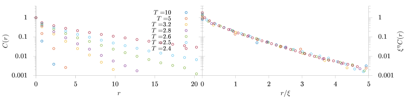
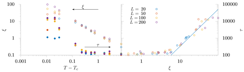
Figure 5: Example of static (top) and dynamic (bottom) scaling in the 2-$d$ Ising model. In the top panel, the space correlation function $C(r)$ was computed using eq. (49) for the Isinng model on a $100\times 100$ square lattice at the specified temperatures. The correlation length $\xi_{2}$ was computed in $k$-space, Eq. (64) fitting the first five points of $C^{-1}(k)$ to a quadratic function. The rightmost plot shows that $\xi^{\eta}C(r)$ plotted vs. $r/\xi$ falls on the same curve for all temperatures. We have used the exact known value $\eta=1/4$. Bottom panel: the correlation length and time (computed with definition (62)) for several temperatures and system sizes grow on approaching $T_{c}$, but saturate at a size-dependent value (left). Right: correlation time vs. correlation length for the same sizes and temperatures as in the left panel, illustrating the dynamic scaling (72). The is a power law with exponent $z=2.21$, value of the dynamic exponent obtained by Münkel et al. (1993).

V.2 Finite-size effects

Scaling laws as written in the previous subsection apply only to infinite systems. Although infinite systems exist only in theory, experimental systems can be considered infinite when $\xi$ is much smaller than the system’s linear size $L$. It is true that when the critical point is approached, $\xi$ will eventually grow to be larger than any system size. However, in condensed matter systems samples are typically many orders of magnitude larger than microscopic lengths, and $\xi$ can be extremely large with respect to inter-particle distances while still being smaller than $L$. The condition $\xi\geq L$ will only be true for a range of temperatures so thin around the critical point that it this effect can in practice be ignored.

In contrast, in experiments in biology the number of units making up the system (aminoacids, cells, organisms) is quite far from the $10^{23}$ or so that condensed matter systems can boast, and the effects of finite size must be properly taken into account. The same is true for numerical simulations, where in fact finite-size effects have long been used (Privman, 1990) to extract information about the critical region. More recently, has also been exploited in experiments on biological systems.

Finite-size effects blur the sharp transitions and singularities that distinguish phase transitions in the thermodynamics of infinite systems. If a critical system is finite, it can be scale invariant only up to the its size $L$; in this sense $L$ acts as an effective correlation length if $\xi>L$. Conversely, if $\xi$ is finite but larger than $L$, the system will appear nevertheless scale invariant. Thus $L$ is finite, scaling relations must be modified to account for the fact that correlations cannot extend beyond $L$. These modified relations are known as finite-size scaling relations (Barber, 1983; Cardy, 1988).

According to the finite-size scaling ansatz (Barber, 1983), when $\xi$ is of the order or greater than $L$ the scaling relations must be modified to include the ratio $L/\xi$. This ansatz can be justified with renormalisation group argouments (Amit and Martín-Mayor, 2006; Cardy, 1988). For the static correlation function, instead of (66) we write

$$C(r) =\frac{1}{r^{d-2+\eta}}f(r/\xi,L/\xi), \text{if }L>\xi,$$ (73)

with $f(x,y)\to f(x)$ for $y\to\infty$, and

$$C(r) =\frac{1}{r^{d-2+\eta}}g(r/L,L/\xi) \text{if }L<\xi,$$ (74)

with $g(x)$ another scaling function.

At the critical point, we are effectively left with a scaling relation of the same type as (66) but with $L$ replacing $\xi$ Cardy (1988),

$$C(r)=\frac{1}{r^{d-2+\eta}}g(r/L)=\frac{1}{L^{d-2+\eta}}\hat{g}(r/L)$$ (75)

(and a different scaling function). Correlations are truly scale-free only in the limit $L\to\infty$, where the scaling function is replaced by a constant. In a finite system, function $g(x)$ will introduce a modulation of the power law when $r\sim L$. Scale invariance manifests instead as a correlation scale that is proportional to $L$: enlarging the system also enlarges the correlation scale. This, together with the fact that the space-averaged correlation function has at least one zero, can be exploited to show that a system is scale-invariant. Calling $r_{0}$ the first zero of $C_{\text{sp}}(r)$, one can show (Cavagna et al., 2018, §2.3.3) that

$$r_{0} \sim\xi\log(L/\xi), L\gg\xi,$$ (76a)

$$r_{0} \sim L, L\ll\xi.$$ (76b)

We emphasise that $r_{0}$ is not in general a correlation length, since it behaves differently: it does not have a finite limit for $L\to\infty$ (even away from the critical point) and it does not scale like $\xi$ with control parameters. However, if $\xi=\infty$, then $r_{0}$ is proportional to $L$ (the only correlation scale). So, if one can show that (76b) holds for a set of systems of different sizes, but otherwise equivalent, one can argue that those systems are in fact scale-free. Such reasoning has been used e.g. in Tang et al. (2017); Cavagna et al. (2010); Attanasi et al. (2014); Fraiman and Chialvo (2012).

In Fourier space, the finite-size version of (68) can be written, for $L<\xi$,

$$\hat{C}(k;L)=k^{-2+\eta}F(kL,L/\xi)=L^{2-\eta}\hat{F}(kL,L/\xi).$$ (77)

The finite-size version of the dynamic scaling law (70) is

$$\tilde{C}(k,t;L)=\tilde{C}(k;L)\hat{h}(t/\tau_{k},kL,L/\xi),\qquad\tau_{k}=k^{-z}\Omega^{-1}(kL,L/\xi)$$ (78)

Then, at the scale-free point $\xi=\infty$ it holds that $\tilde{C}(k,t;L)$ measured for systems of different size depends on $k^{z}t$ if one measures each system at a $k$ such that $kL=\text{const}$. This scaling law has been successfully applied to study the dynamical behaviour of swarms of midges in the field (Cavagna et al., 2017). For the global relaxation time one has, instead of (72)

$$\tau=L^{z}\hat{\Omega}^{-1}(L/\xi).$$ (79)

To conclude, let us point out that from what we have said it follows that a single measurement of $\xi$ on a finite system does not tell one anything about whether correlations are long range or not. An unknown numerical prefactor is involved in the estimation of $\xi$, and the estimators we have discussed tend to be less reliable when $\xi\sim L$, so that it does not make sense to discuss whether, say, is $\xi=L/2$ large or not. Instead, it is necessary to measure the trend of $\xi$ with control parameters, and if at all possible, with $L$. Moreover, studying different system sizes can show whether the correlation scale grows with $L$ and establish that the system is scale-free in situations where changing the control parameters is not feasible.

There can be situations, especially in biological experiments, where changing system size is not possible (e.g. how would one study human brains of different sizes?). In such circumstances, one may attempt to do finite-size scaling by measuring subsystems (“boxes”) of size $W\ll L$ and studying how the quantities change when varying $W$. The idea can be traced back to Binder (1981), and has also been employed out of equilibrium (Fernández and Martín-Mayor, 2015). The applicability of relations (76) with the box size $W$ in place of $L$ for systems of fixed size was recently demonstrated for several simulated systems (Martin et al., 2020).

VI Space-time correlations in neuronal networks

The finding of scale-free avalanches in cortical tissue (Beggs and Plenz, 2003; Shew et al., 2009) and strong correlations in retinal cells (Schneidman et al., 2006; Tkačik et al., 2006, 2015) are early experimental evidence of criticality in neuronal populations (see Mora and Bialek (2011) and Chialvo (2010) for reviews of these and more recent experiments). At the level of the whole brain, fMRI measurements of neuronal activity (Expert et al., 2011; Fraiman and Chialvo, 2012; Tagliazucchi et al., 2012) have found long-range correlation, providing support for the conjecture that the brain operates at a critical point (Bak, 1996; Chialvo and Bak, 1999; Beggs, 2008).

Notwithstanding the importance of these works in forwarding our understanding of how complex behaviour can arise in the brain, it is fair to say that the picture of the brain as a critical system is still work in progress, and surely new experiments will be attempted in the near future. Critical systems display distinctive dynamic, as well as static characteristics, and much information can potentially be gained by studying systematically static and dynamic correlations together on the same system, and in particular the scaling relations. For instance, study of static correlations in midge mating swarms using finite-size scaling led to the finding (Attanasi et al., 2014) that they are in a critical regime compatible with the critical Vicsek model (Vicsek et al., 1995). A subsequent investigation of dynamic correlations in the same system showed that they obey dynamic scaling (Cavagna et al., 2017), but with a novel dynamic exponent, incompatible with the dynamics of the Vicsek model. The exponent turned out to be different from those of the classical dynamic models (Hohenberg and Halperin, 1977), and this spurred still-ongoing efforts to understand whether a combination of inertia and activity ingredients can explain this new exponent (Cavagna et al., 2019).

Clearly, magnets, swarms and brains are quite different systems, and in particular the special network structure of neuronal assemblies poses specific problems (Korchinski et al., 2021). Certainly it is not the case to take tools developed in the statistical mechanics of condensed matter and blindly apply them to study the brain. But knowledge of other critical systems suggests the relation between correlation time and length scales can hold valuable information. The question calls for an experimental study, but we wish to conclude this article with an exploration of a simple excitable network model, which can serve as some illustration to the exposition of correlation functions, and hopefully stir up interest for experimental studies of length and time correlation scales in the brain.

VI.1 The ZBPCC model

We study the simple neural network model proposed by Zarepour et al. (2019), which is essentially the model used by Haimovici et al. (2013) but implemented on a small-world network. The dynamics is that of a Greenberg-Hastings cellular automaton Greenberg and Hastings (1978), where each site of the network has three possible states, $S_{i}=\{Q,E,R\}$, corresponding to quiescent, excited or refractory, respectively, and the transitions among them are ruled by the probabilities

$$P_{i,Q\to E} =1-\bigl{[}1-r_{1}\bigr{]}\left[1-\Theta\left(\sum_{j}W_{ij}\delta_{S_{j},E}-T\right)\right],$$ (80a)

$$P_{i,E\to R} =1,$$ (80b)

$$P_{i,R\to Q} =r_{2}.$$ (80c)

$P_{i,a\to b}$ is the probability that site $i$ will transition from $a$ to state $b$, $\Theta(x)$ is Heaviside’s step function [$\Theta(x)=1$ for $x\geq 0$ or 0 otherwise], $\delta_{i,j}$ is Kronecker’s delta, $r_{1}$, $r_{2}$ and $T$ are numeric parameters and $W_{ij}$ is the network’s connectivity matrix (see below). Thus an active site always turns refractory in the next time step, and a refractory site becomes quiescent with probability $r_{2}$. We set $r_{2}=0.3$ as in previous work (Zarepour et al., 2019; Haimovici et al., 2013), so that the site remains refractory for a few time steps, and $r_{1}=10^{-6}$ so that external excitation events are relatively rare. The probability for a quiescent site to become active is written as 1 minus the product of the probabilities of not becoming active through the two mechanisms at work: spontaneous activation, which occurs with a small probability $r_{1}$ (mimicking an external stimulus), or transmitted activation, which occurs with certainty if the sum of the weights of the links connecting $i$ to its active (excited) neighbours exceeds a threshold $T$. All sites are updated simultaneously.

The model runs on an undirected weighted graph described by the connectivity matrix elements $W_{ij}\geq 0$, where a nonzero element means a bond with the specified weight connects sites $i$ and $j$, and $W_{ij}=W_{ji}$. Neither the connectivity nor the weights depend on time. The graph is a bidirectional Watts-Strogatz small-world network (Watts and Strogatz, 1998) with average connectivity $\langle k\rangle$ and rewiring probability $\pi$. The network is constructed as usual (Watts and Strogatz, 1998) by starting from ring of $N$ nodes, each connected symmetrically to its $\langle k\rangle/2$ nearest neighbours; then each link connecting a node to a clockwise neighbour is rewired to a random node with probability $\pi$, so that average connectivity is preserved. The rewiring probability is a measure of the disorder in the network; $\pi=0$ preserves the original network topology, while $\pi=1$ gives a completely random graph. Once the network bonds are drawn, each is assigned a random weight drawn from an exponential distribution, $p(W_{ij}=w)=\lambda e^{-\lambda w}$, with $\lambda=12.5$ chosen to mimic the weight distribution of the human connectome (Zarepour et al., 2019)

The simplest way to characterise the state of the network is perhaps the activity order parameter, i.e. the fraction of active sites

$$a=\frac{1}{N}A,\qquad A=\sum_{i}\delta_{S_{i},E}.$$ (81)

By analogy to magnetic systems, one can define an associated susceptibility, proportional to the variance of $a$,

$$\chi=\frac{1}{N}\left[\langle A^{2}\rangle-\langle A\rangle^{2}\right],$$ (82)

where $\langle\ldots\rangle$ is a time average. Another possible characterisation is by studying the percolation of active clusters, as in Zarepour et al. (2019). The percolation order parameter is the probability that a site belongs to the largest cluster,

$$P_{\infty}=\frac{1}{N}S_{1},$$ (83)

where $S_{1}$ is size of the largest active cluster, i.e. the number of sites that belong to the largest connected component of the graph of active sites. The quantity that plays a role analogous to $\chi$ is the mean (finite) cluster size Stauffer and Aharony (1994),

$$S=\frac{\sum^{\prime}_{s}s^{2}N_{s}}{\sum^{\prime}_{s}sN_{s}},$$ (84)

where $N_{s}$ is the number of clusters of size $s$, the sum is over all possible values of $s$ and the prime means that the largest cluster is excluded.

These quantities were computed as a function of $T$ for $\pi=0.2$ and average connectivity $\left\langle K\right\rangle=12$ and $\left\langle K\right\rangle=6$ (Fig. 6). At this value of $\pi$, $\left\langle K\right\rangle=6$ lies in the “no transition” region, while $\left\langle K\right\rangle=12$ is in the continuous transition region of $(\pi,\left\langle K\right\rangle)$ space according to Fig. 4 of Zarepour et al. (2019). Indeed we find $\left\langle K\right\rangle=12$ shows a clear percolation transition (Fig. 6 bottom left), with a peak in $S$ that grows with system size and $P_{\infty}$ that goes to zero more and more sharply at $T_{p}\approx 0.15$. Instead for $\left\langle K\right\rangle=6$ no transition is observed, and $P_{\infty}$ becomes progressively flatter as $N$ is increased (Fig. 6 bottom right).

However, study of percolation requires knowledge of network connectivity, which may be difficult to obtain experimentally. A simpler approach is to measure the average activity, without regards to connectivity. Using $a$ as order parameter one obtains a different picture: both cases appear to have a continuous transition, where activity goes smoothly to zero at $T_{a}\approx 0.19$ for $\left\langle K\right\rangle=12$ and at $T_{a}\approx 0.12$ for $\left\langle K\right\rangle=6$. The transition is however unusual in that $\chi$ has a (not very sharp) maximum at a different value of $T$, and the height of the peak in $\chi$ does not scale with size (i.e. unlike usual second order transitions, here $\chi$ never diverges). We have found no sign of the two transition thresholds $T_{p}$ and $T_{a}$ moving toward each other, up to our maximum network size of $10^{6}$ nodes.

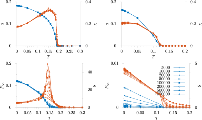
Figure 6: Dynamic transition of the ZBPCC model on the Watts-Strogatz small world network with average connectivity $\left\langle K\right\rangle=12$ (left column) and $\left\langle K\right\rangle=6$ (right column). Top: activity (blue) and susceptibility (orange) vs. threshold level $T$. Bottom: percolation order parameter $P_{\infty}=S_{1}/N$ (blue) and mean cluster size $S$ (orange) vs $T$. Symbol type indicates the network size. Curves are obtained after averaging over 2 to 10 realisations of the network. Sizes are $N=5\cdot 10^{3}$, $10^{4}$, $2\cdot 10^{4}$, $5\cdot 10^{4}$, $10^{5}$, $2\cdot 10^{5}$, $5\cdot 10^{5}$ and $10^{6}$. In all cases $\pi=0.2$, $r_{1}=10^{6}$, $r_{2}=0.3$.

Which of the two transitions should we pay attention to? In a sense both are complementary, since they reveal different aspects of the network activity. However, a study of time correlations shows that the activity transition, though less well-behaved from the static point of view, is more relevant dynamically. We have computed the time correlation function of both order parameters ($A/N$ and $S_{1}/N$), and the corresponding correlation times $\tau_{a}$ and $\tau_{s}$ defined according to (62) (see Fig. 7). The correlation time of the activity, $\tau_{a}$, shows a peak that grows with system size at the activity transition $T_{a}$, while the correlation time $\tau_{s}$ has a broader peak also near $T_{a}$, but it does not grow with $N$. A similar situation is found looking at the normalised time correlation function after one step, $C_{c}(t=1)$, a quantity which peaks at a regular second order phase transition (Chialvo et al., 2020): when computed for the activity, it displays a clear peak at $T_{a}$, while when computed for the largest cluster size it shows, for large systems, two small peaks, near $T_{a}$ and near $T_{P}$, although it is not clear whether these will survive the thermodynamic limit.

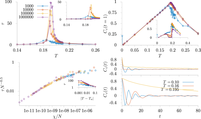
Figure 7: Correlation time and correlation function on the ZBPCC model for $\left\langle K\right\rangle=12$ (corresponding to the right column of Fig. 6). The relaxation time of the activity order parameter has a peak at the activity transition $T_{a}$ (top left), while no peak is observed near $T_{P}$, even in the correlation time of the percolation order parameter $S_{1}/N$ (top left inset). Symbol colour indicates system size. $C_{c}(t=1)$ also has a peak at $T_{a}$ (top right) when computed for the activity, while for $S_{1}/N$ two small peaks seem to develop at large $N$ (top right). The maximum correlation time $\tau_{a}$ grows with system size (bottom left inset) and can be scaled against $\chi/N$ (bottom left). The time correlation function of the activity is damped oscillatory below $T_{a}$ but does not oscillate above $T_{a}$ (lower plot, bottom right), and the same for the correlation of $S_{1}/N$ above and below $T_{p}$ (upper plot, bottom right).

At both transitions, the shape of the time correlation of the respective order parameter changes, with damped oscillations found at low $T$ giving way to an overdamped-like decay at higher $T$ (lower right panel of Fig. 7).

The plot of $\tau_{a}$ vs. $T$ shows a peak that grows with system size, with curves of $\tau_{a}$ vs. $\lvert T-T_{a}\rvert$ saturating at higher values for larger systems. Unfortunately, it is not possible to explore standard dynamic scaling in this model, because it is defined on a graph with no spatial structure, so that space correlations cannot be defined. We make an attempt using $\chi$ (which in a ferromagnetic transition would scales with a power of $\xi$, although here it never diverges). Somewhat surprisingly, a reasonable scaling behaviour is obtained plotting $N^{-1/2}\tau$ vs $\chi/N$, i.e. the variance of $a$.

VI.2 ZBPCC on the fcc lattice

We explore the simplest strategy to endow the ZBPCC model with a spatial structure: we build a graph connecting the nearest neighbours of a regular lattice, and then rewire it with probability $\pi$ as in the small world case. We chose the face-centred cubic (fcc) lattice, which has connectivity $K=12$, the same value where for the small-world case we found both activity and percolation transitions.

Fig. 8 shows the behaviour of the activity and percolation order parameters for the pure fcc lattice ($\pi=0$) and for the fcc lattice rewired with $\pi=0.2$. The fcc lattice shows a situation similar to the small world network with $\left\langle K\right\rangle=6$, with a transition in $a$ but no percolation transition. The maximum of $\chi$ is shifted with respect to $T_{a}$. The rewired fcc lattice instead shows both the activity and percolation transitions, in this case with the maximum of $\chi$ very close to $T_{a}$. Here $T_{P}\approx 0.17$. In both cases $T_{a}\approx 0.19$. These results suggest that $T_{a}$ depends mainly on the network connectivity, while the percolation transition is more sensitive to the details of network topology.

Note that the threshold for random site percolation on the fcc lattice place the percolation transition at has been estimated at an occupation probability of $p_{c}\approx 0.199$ (van der Marck, 1998; Xu et al., 2014). The recorded network activity is always below $0.190$, so that, if active sites were distributed at random, one would not expect a percolating cluster to form. The fact that an infinite cluster appears for $\pi=0.2$ at about $a\approx 0.094$ means that active sites must be more clustered than would result from random activation.

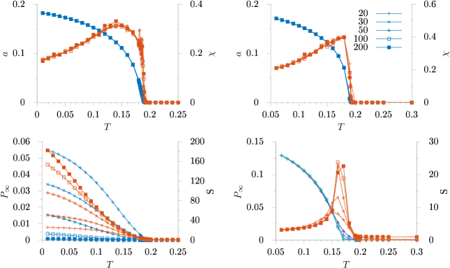
Figure 8: ZBPCC on the fcc lattice (left column) and on the fcc lattice rewired with $\pi=0.2$ (right column). Top row: activity $a$ (blue) and susceptibility $\chi$ (orange); bottom row: $P_{\infty}$ (blue) and $S$ (orange).

In this version of the model we can use the underlying fcc lattice to define distances and compute space correlations. We have computed $C(k)$ and used it to compute $\xi_{2}$ with definition (64) and a quadratic fit at small $k$ (see Fig. 9). For $\pi=0$ the largest $\xi$ is about a tenth of the lattice size, and finite-size effects are modest. On the contrary, on the rewired fcc, there is a strong size effect. However, instead of the situation usual in a regular lattice, with $\xi$ vs. $T$ curves superimposing at high $T$ and saturating at different values on approaching the critical point (see Fig. 5), here $\xi$ grows with $L$ almost uniformly for all $T$, and the $\xi$ vs $T$ seem to scale when dividing by $L$ (Fig. 9, inset of top right panel). Given that this effect only appears with rewiring, it may be related to the fact that when a link is rewired, the new neighbour is chosen randomly over all the nodes without regards to the distance, a procedure that is not very realistic.

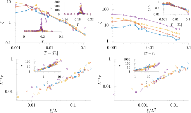
Figure 9: ZBPCC on the fcc lattice (left column) and the fcc rewired with $\pi=0.2$ (right column). The correlation length and time have a peak at $T_{a}$ (top left). In the case of the rewired network, $\xi$ has a strong dependence on lattice size, indicated by symbol color (top right). Bottom row: relationship between $\tau$ and $\xi$.

Finally we have computed the correlation time of the activity. This shows a size-dependent maximum at $T_{a}$ in both cases, confirming the dynamical relevance of $T_{a}$. Comparing $\tau_{a}$ and $\xi$ shows that both grow together, but the attempt at applying dynamic scaling (bottom panels of Fig. 9) is not very satisfactory. A more detail analysis is needed of the role played by topological details and network disorder.

VII Conclusions

We have discussed how space (static), time (dynamic), and space-time correlation functions can be defined and computed in a variety of situations, how characteristic correlation length and times are computed, and summarised our knowledge of scaling relations and finite-size effects for systems near a critical point. We have finally applied these tools to analyse the dynamic transition of the simple ZBPCC neuronal model, as well as a variant thereof introducing a simple spatial structure. Studying the time correlations of the two order parameters considered showed that only the activity correlation time has a peak, thus hinting that the activity transition is more relevant for the description of the model dynamics. The fcc version of the ZBPCC proposed here showed a correlation length that also peaks at the activity transition, but with an unusual finite-size behaviour, especially in the rewired case. The way space has been introduced in the model is however somewhat artificial, and it is worthwhile to consider models with realistic spatial structure and connectivity, implementing a simple excitable model like the Greenberg-Hastings but on the human connectome, as in Haimovici et al. (2013) or Ódor (2016). Work in this direction is in progress.

I thank D. Chialvo for helpful discussions on the ZBPCC model, and for bringing some references to my attention. I also thank A. Cavagna and I. Giardina, who over a long collaboration helped shape my understanding of concepts and practicalities of correlation functions, especially as applied to biological systems. This work was supported in part by grants from Universidad Nacional de La Plata and Consejo Nacional de Investigaciones Científicas y Técnicas (CONICET, Argentina).

Appendix A Stochastic processes

A stochastic process, or sometimes random field, is a family of random variables indexed by $\mathbf{r}$ and $t$. Thus there must exist a family of probability densities $P(a,\mathbf{r},t)$ that allows to compute all moments $\left\langle a^{n}(\mathbf{r},t)\right\rangle$ and in general any average $\left\langle f\bigl{(}a(\mathbf{r},t)\bigr{)}\right\rangle$. But $P(a,\mathbf{r},t)$ is not enough to characterise the stochastic process, because in general the variables $a(\mathbf{r},t)$ at different places/times will not be independent. Thus $P(a,\mathbf{r},t)$ is actually a marginal distribution of some more complicated multivariate probability density.

A complete characterisation of the stochastic process would need an infinite-dimensional probability distribution $P\bigl{[}a(\mathbf{r},t)\bigr{]}$ that gives the joint probability for all random variables $a(\mathbf{r},t)$. However, one can usually avoid the difficulties associated with such a distribution by considering the set of $n$-variable joint distributions

$$P_{n}(a_{1},\mathbf{r}_{1},t_{1},a_{2},\mathbf{r}_{2},t_{2},\ldots,a_{n},\mathbf{r}_{n},t_{n}).$$ (85)

Most stochastic processes (Priestley, 1981, §3.2.1) can be completely specified by the set of all joint probabilities of the form (85) for all $n$ and all possible choices of $\mathbf{r}_{1},t_{1},\ldots,\mathbf{r}_{n},t_{n}$. This should include all processes of interest in physics and biology. To define two-point correlation functions we need only the set corresponding to $n=2$ (7), which gives also the set for $n=1$ by marginalising on the second variable.

The joint probability distributions that define the process are time-translation invariant (TTI) if they obey (we omit the space variables for clarity)

$$P_{n}(A_{1},t_{1},\ldots,A_{n},t_{n})=P(A_{1},t_{1}+s,\ldots,A_{n},t_{n}+s)$$ (86)

for all times, $s$ and $n$. Stochastic processes obeying TTI are called completely stationary processes. A related but less restrictive notion is that of stationary processes up order $M$, defined by the requirement that all the joint moments up to order $M$ exist and are time-translation invariant:

$$\left\langle A^{m_{1}}(t_{1})A^{m_{2}}(t_{2})\ldots A^{m_{n}}(t_{n})\right\rangle=\langle A^{m_{1}}(t_{1}+s)A^{m_{2}}(t_{2}+s)\ldots A^{m_{n}}(t_{n}+s)\rangle$$ (87)

for all $s$, $n$, $\{t_{1},\ldots,t_{n}\}$ and $\{m_{1},\ldots,m_{n}\}$ such that $m_{1}+m_{2}+\ldots+m_{n}\leq M$. This is less restrictive not only because of the bound on the number of random variables considered, but also because invariance is imposed only on the moments, and not on the joint distributions themselves.

Appendix B The estimator $\hat{C}^{(c)}_{k}$ always has a zero

An important property of estimator (37) will always have zero, whatever the length of the sequence used to compute it. To see this, consider the quantity

$$B_{i}=(N-i)\hat{C}_{c,i}=\sum_{j=1}^{N-i}\delta a_{j}\delta a_{j+i},$$ (88)

and compute the sum

$$\sum_{i=0}^{N-1}B_{i}=\sum_{i=0}^{N-1}\sum_{j=1}^{N-i}\delta a_{j}\delta a_{j+i}=\sum_{i=0}^{N-1}\sum_{j=1}^{N}\sum_{k=1}^{N}\delta a_{j}\delta a_{k}\delta_{k,j+i}.$$ (89)

But $\sum_{i=0}^{N-1}\delta_{k,j+i}$ equals 1 if $k\geq j$ and 0, so

$$\sum_{i=0}^{N-1}B_{i}=\sum_{j=1}^{N}\sum_{k=j}^{N}\delta a_{j}\delta a_{k}=\frac{1}{2}\sum_{j\neq k}^{N}\delta a_{j}\delta a_{k}+\sum_{j=1}^{N}(\delta a_{j})^{2}=\\ \frac{1}{2}\left[\sum_{j=1}^{N}\delta a_{j}\right]^{2}+\frac{1}{2}\sum_{j=1}^{N}(\delta a_{j})^{2}=\frac{1}{2}\sum_{j=1}^{N}(\delta a_{j})^{2}>0,$$ (90)

where the last equality follows because $\sum_{j}\delta a_{j}=0$. Now we can easily do the same sum starting from $i=1$:

$$\sum_{i=1}^{N-1}B_{i}=-B_{0}+\sum_{i=0}^{N-1}B_{i}=-\frac{1}{2}\sum_{j=1}^{N}(\delta a_{j})^{2}<0.$$ (91)

This shows that at least some of the $B_{i}$ must be negative. But since $B_{0}>0$, the conclusion is that $B_{k}$, and hence $\hat{C}_{c,k}$, which differs from it by a positive factor, must change sign at least once for $k\geq 1$.

Appendix C The shape of the correlation decay

Fig. 10 illustrates several (simple) possible shapes of a decaying function. It should make it clear why a threshold to define a correlation scale is misleading unless the curves to be compared are all the same shape. Apart from the simple exponential $\rho(t)=e^{t/\tau}$ and the sum of exponentials, the figure illustrates two interesting cases.

One is the Kolrausch-William-Watts functions (lower left panel),

$$\rho_{\text{\tiny K}}(t)=e^{-(t/\tau_{\text{\tiny K}})^{\beta}},$$ (92)

a function widely used to describe non-exponential decays, employing only three parameters. Here $\tau_{\text{\tiny K}}$ is a time scale and $\beta$ is the stretching exponent: the KWW function gives a stretched exponential for $\beta<1$, and a compressed exponential for $\beta>1$. Definition (57) gives 0 in the compressed case, and $\infty$ in the stretched case. This can be understood considering the decay as a superposition of exponential processes,

$$\rho_{\text{\tiny K}}(t)=\int_{0}^{\infty}w(\tau)e^{-t/\tau}\,d\tau,$$ (93)

which defines the correlation time distribution function $w(\tau)$. It can be seen that the support of $w(\tau)$ extends to infinity for $\beta<1$ Lindsey and Patterson (1980). The integral correlation time is instead more useful here,

$$\tau_{\text{int}}=\frac{\tau_{\text{\tiny K}}}{\beta}\Gamma\left(\frac{1}{\beta}\right),$$ (94)

where $\Gamma(x)$ is Euler’s gamma function. So $\tau_{\text{int}}$ is proportional to $\tau_{\text{\tiny K}}$, but $\tau_{\text{int}}$ incorporates information about the shape of the tail of the decay, making it better suited to compare two decays with different $\beta$.

The other case is that of damped oscillations, that appear in systems with important inertial effects. In the simplest harmonic form we have

$$\rho_{\text{\tiny osc}}(t)=e^{t/\tau}\cos(\omega_{0}t).$$ (95)

The integral (58) and spectrum (62) scales are

$$\tau_{\text{int}} =\frac{\tau}{1+(\omega_{0}\tau)^{2}}, \tau_{0} =\frac{\tau}{\sqrt{1+(\omega_{0}\tau)^{2}}}.$$ (96)

In the overdamped case, $\omega_{0}\tau\ll 1$ both scales tend to $\tau$, but in the opposite limit $\omega_{0}\tau\gg 1$, where the function oscillates many times before significant damping is observed, $\tau_{\text{int}}\sim 0$ while $\tau_{0}\sim 1/\omega_{0}$.

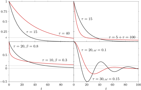
Figure 10: Different possible shapes for the decay of the time correlation. Top left: simple exponential. Top right: simple exponential (black curve) and double exponential (red curve) decay. In this case, the threshold criterion (here $\epsilon=0.1$) labels the red curve as the fastest, but it clearly has a longer tail. Bottom left: stretched exponential. The integral correlation time (58) is $\tau_{\text{int}}\approx 22.7$ (black curve), $\tau_{\text{int}}\approx 92.6$ (red curve). Bottom right: exponentially damped harmonic oscillations.

Appendix D Algorithms to compute time correlations

The estimators can be computed numerically by straightforward implementation of equations (35) or (37), although in the stationary case it is much more efficient to compute the connected correlation through relation (31) using a fast Fourier transform (FFT) algorithm. Let us focus on the stationary case and examine in some detail these algorithms.

Algorithm 1 presents the direct method. It is straightforward to translate the pseudo-code to an actual language of your choice. Apart from some missing variable declarations, the only thing to consider is that it is probably inconvenient (or even illegal, as in classic C) to return a large array, and it is better to define $C$ as an output argument, using a pointer or reference (as e.g. FORTRAN or C do by default) to avoid copying large blocks of data. The advantages of this algorithm are that it is self-contained and simple to understand and implement. Its main disadvantage is that, due to the double loop of lines 8–11, it runs in a time that grows as $N^{2}$. For $N$ up to about $10^{5}$, algorithm 1 is perfectly fine: a good implementation in a compiled language should run in a few seconds in a modern computer. But this time grows quickly; in the author’s computer $N=5\cdot 10^{5}$ takes 35 seconds, for $N=10^{6}$ the time is two and a half minutes. In contrast, the algorithm with FFT takes 1 second for $N=10^{6}$ and 11 seconds for $N=10^{7}$.

Algorithm 1 Compute the connected correlation of sequence $a$ (of length $N$) using the direct $O(N^{2})$ method. The connected correlation is returned in vector $C$.

1:function timecorr($a$,$N$)

2:     $\mu\leftarrow 0$ $\triangleright$ Compute average

3:     for $i=1,\ldots,N$ do

4:         $\mu\leftarrow\mu+a_{i}$      

5:     $\mu\leftarrow\mu/N$

6:     for $i=1,\ldots,N$ do $\triangleright$ Clear $C$ vector

7:         $C_{i}\leftarrow 0$      

8:

9:     for $i=1,\ldots,N$ do $\triangleright$ Correlation loop

10:         $d\leftarrow a_{i}-\mu$

11:         for $k=0,\ldots,N-i$ do

12:              $C_{k+1}\leftarrow C_{k+1}+d*(a_{i+k}-\mu)$               

13:

14:     for $i=1,\ldots,N$ do $\triangleright$ Normalize and return

15:         $C_{i}\leftarrow C_{i}/(N-i-1)$      

16:     return C

If the correlation of really long sequences is needed, the FFT-based algorithm, though more difficult to get running, pays off with huge savings in CPU time at essentially the same numerical precision. The idea of the algorithm is to compute the Fourier transform of the signal, use (30) to obtain the Fourier transform of the connected correlation, then transform back to obtain $C_{c}(t)$. This is faster than algorithm 1 because the clever FFT algorithm can compute the Fourier transform in a time that is $O(N\log N)$.

Actually, we need discrete versions of the Fourier transform formulas (as we remarked before, the Fourier transform of the continuous time signal does not exist). The discrete Fourier transform (DFT) and its inverse operation are defined (Press et al., 1992, §12.1) as (it is convenient to let the subindex of $a_{i}$ run from $0$ to $N-1$ to write the following two equations),

$$\tilde{a}_{k}=\sum_{j=0}^{N-1}e^{2\pi ijk/N}a_{j},\qquad a_{j}=\frac{1}{N}\sum_{k=0}^{N-1}e^{-2\pi ijk/N}\tilde{a}_{k},$$ (97)

where we note that the inverse DFT effectively extends the sequence periodically (with period $N$). The discrete version of (30) is (Press et al., 1992, §13.2)

$$\tilde{D}_{k} =|\tilde{a}_{k}|^{2}, D_{j} =\sum_{k=0}^{N-1}a_{k}a_{k+j},$$ where (98)

and where the definition of $D_{j}$ makes use of the (assumed) periodicity of $a_{i}$. $D_{j}$ is almost our estimate (37): we only need to take care of the normalization and of the fact that due to the assumed periodicity of $a_{i}$ some past times are regarded as future, e.g. for $k=10$, in the sum there appear the terms $a_{0}a_{10}$ up to $a_{N-11}a_{N-1}$ (which are fine), but also $a_{N-10}a_{0}$ through $a_{N-1}a_{9}$, which we do not want included. This is fixed by padding the original signal with $N$ zeros at the end, i.e. setting $a_{k}=0$ for $k=N,\ldots,2N-1$ and ignoring the values of $D_{j}$ for $j\geq N$.

In summary, to compute the connected correlation using FFT the steps are i) estimate the mean and substract from the $a_{i}$, ii) add $N$ zeros to the end of the sequence, iii) compute the DFT of the sequence, iv) compute the squared modulus of the transform, iv) compute the inverse DFT of the squared modulus, v) multiply by the $1/(N-i)$ prefactor. Pseudocode for this algorithm is presented as algorithm 2.

Algorithm 2 Compute the connected correlation of sequence $a$ (of length $N$) using a fast Fourier transform. This algorithm is $O(N\log N)$.

1:function timecorr($a$,$N$)

2:     $\mu\leftarrow 0$ $\triangleright$ Compute average

3:     for $i=1,\ldots,N$ do

4:         $\mu\leftarrow\mu+a_{i}$      

5:     $\mu\leftarrow\mu/N$

6:     for $i=0,\ldots,N$ do $\triangleright$ Substract the average from signal

7:         $a_{i}\leftarrow a_{i}-\mu$      

8:     for $i=N,\ldots,2N$ do$\triangleright$ Pad with 0s at the end

9:         $\text{a}_{i}\leftarrow 0$      

10:

11:     $b\leftarrow$FFT($a$,$2N$) $\triangleright$ Compute the FFT of a as a vector of length $2N$

12:     for $i=1,\ldots,2N$ do $\triangleright$ Compute squared modulus of $b$

13:         $b_{i}\leftarrow\lvert b_{i}\rvert^{2}$ $\triangleright$ Note that the Fourier transform is complex      

14:     $C\leftarrow$IFFT($b$,$2N$) $\triangleright$ Inverse FFT

15:

16:     $C\leftarrow$resize($C$,$N$) $\triangleright$ Discard the last $N$ elements of $C$

17:     for $i=1,\ldots,N$ do $\triangleright$ Normalize and return

18:         $\text{C}_{i}\leftarrow\text{C}_{i}/(N-i-1)$      

19:     return C

To translate this into an actual programming language the comments made for algorithm 1 apply, and in addition some extra work is needed for lines 10–13. First, one needs to choose an FFT routine. The reader curious about the FFT algorithm can read for example (Press et al., 1992, Ch. 12) or Duhamel and Vetterli (1990), but writing an FFT routine is not easy, and implementing a state-of-the-art FFT is stuff for professionals. Excellent free-software implementations of the FFT can be found on Internet. FFTW Frigo and Johnson (2005), at http://www.fftw.org deserves mention as particularly efficient, although it is a large library and a bit complex to use. Note that some simpler implementations require that $N$ be a power of two, failing or using a slow $O(N^{2})$ algorithm if the requiriment is not fulfilled. Also pay attention to i) the difference between “inverse” and “backward” DFTs (the latter lacks the $1/N$ factor), ii) how the routine expects the data to be placed in the input array, iii) how it is returned, and iv) whether the transform is done “in place” (i.e. overwriting the original data) or not. If the routine is a “complex FFT” it will expect complex input data (so that for real sequences you will have to set to zero the imaginary part of the $a_{i}$), while if it is a “real FFT” routine it will typically arrange (“pack”) the output data in some way, making use of the discrete equivalent of the $\tilde{A}(-\omega)=A^{*}(\omega)$ symmetry so as to return $N$ real numbers instead of $2N$. This affects the way one must compute the squared modulus (lines 11–12). For example, for the packing used by the FFTW real routines, lines 11–12 translate to (in C)

⬇

b[0]*=b[0];

for (int i=1; i<N; i++) {

b[i] = b[i]*b[i] + b[2*N-i]*b[2*N-i];

b[2*N-i] = 0;

}

b[N]*=b[N];

References

- Allen and Tildesley (1987) Allen, M. P., and D. J. Tildesley, 1987, Computer Simulation of Liquids (Clarendon Press, Oxford).
- Amit and Martín-Mayor (2006) Amit, D. J., and V. Martín-Mayor, 2006, Field Theory, the Renormalization Group, and Critical Phenomena: Graphs to Computers (World Scientific), third edition, ISBN 981-256-119-6.
- Ashcroft and Mermin (1976) Ashcroft, N. W., and N. D. Mermin, 1976, Solid State Physics (Cengage Learning).
- Attanasi et al. (2014) Attanasi, A., A. Cavagna, L. Del Castello, I. Giardina, S. Melillo, L. Parisi, O. Pohl, B. Rossaro, E. Shen, E. Silvestri, and M. Viale, 2014, Phys. Rev. Lett. 113(23), 238102, ISSN 0031-9007, 1079-7114.
- Bak (1996) Bak, P., 1996, How Nature Works: The Science of Self-Organized Criticality (Copernicus), ISBN 978-0-387-94791-4.
- Barber (1983) Barber, M. N., 1983, in Phase Transitions and Critical Phenomena, edited by C. Domb and J. L. Lebowitz (Academic Press, London), volume 8, pp. 145–266.
- Beggs (2008) Beggs, J. M., 2008, Philos. Trans. R. Soc. Math. Phys. Eng. Sci. 366(1864), 329.
- Beggs and Plenz (2003) Beggs, J. M., and D. Plenz, 2003, J. Neurosci. 23(35), 11167, ISSN 0270-6474, 1529-2401.
- Binder (1981) Binder, K., 1981, Z. Physik B - Condensed Matter 43(2), 119, ISSN 1431-584X.
- Binney et al. (1992) Binney, J. J., N. J. Dowrick, A. J. Fisher, and M. E. J. Newman, 1992, The Theory of Critical Phenomena: An Introduction to the Renormalization Group (Clarendon Press), ISBN 978-0-19-851393-3.
- Caracciolo et al. (1993) Caracciolo, S., R. G. Edwards, A. Pelissetto, and A. D. Sokal, 1993, Nuclear Physics B 403(1), 475, ISSN 0550-3213.
- Cardy (1988) Cardy, J. (ed.), 1988, Finite-Size Scaling, number 2 in Current Physics Sources and Comments (North-Holland, Amsterdam).
- Cardy (1996) Cardy, J., 1996, Scaling and Renormalization in Statistical Physics (Cambridge University Press).
- Cavagna et al. (2010) Cavagna, A., A. Cimarelli, I. Giardina, G. Parisi, R. Santagati, F. Stefanini, and M. Viale, 2010, Proc. Natl. Acad. Sci. 107(26), 11865, ISSN 0027-8424, 1091-6490.
- Cavagna et al. (2017) Cavagna, A., D. Conti, C. Creato, L. Del Castello, I. Giardina, T. S. Grigera, S. Melillo, L. Parisi, and M. Viale, 2017, Nature Phys. 13(9), 914, ISSN 1745-2473.
- Cavagna et al. (2019) Cavagna, A., L. Di Carlo, I. Giardina, L. Grandinetti, T. S. Grigera, and G. Pisegna, 2019, Phys. Rev. Lett. 123(26), 268001.
- Cavagna et al. (2018) Cavagna, A., I. Giardina, and T. S. Grigera, 2018, Physics Reports 728, 1, ISSN 0370-1573.
- Cavagna et al. (2012) Cavagna, A., T. S. Grigera, and P. Verrocchio, 2012, J. Chem. Phys. 136(20), 204502, ISSN 00219606.
- Chialvo (2018) Chialvo, D., 2018, Acta Phys. Pol. B 49(12), 1955, ISSN 0587-4254, 1509-5770.
- Chialvo (2010) Chialvo, D. R., 2010, Nat. Phys. 6(10), 744, ISSN 1745-2473, 1745-2481.
- Chialvo and Bak (1999) Chialvo, D. R., and P. Bak, 1999, Neurosience 90(4), 1137.
- Chialvo et al. (2020) Chialvo, D. R., S. A. Cannas, T. S. Grigera, D. A. Martin, and D. Plenz, 2020, Sci. Rep. 10(1), 1, ISSN 2045-2322.
- Cooper et al. (1982) Cooper, F., B. Freedman, and D. Preston, 1982, Nucl Phys B 210, 210.
- Cugliandolo (2004) Cugliandolo, L. F., 2004, in Slow Relaxations and Nonequilibrium Dynamics in Condensed Matter, edited by J.-L. Barrat, M. Feigelman, and J. Kurchan (Springer), number LXXVII in Les Houches Summer School, p. 367.
- De Palo et al. (2017) De Palo, G., D. Yi, and R. G. Endres, 2017, PLOS Biol. 15(4), e1002602, ISSN 1545-7885.
- Dombrowski et al. (2004) Dombrowski, C., L. Cisneros, S. Chatkaew, R. E. Goldstein, and J. O. Kessler, 2004, Phys. Rev. Lett. 93(9), 098103.
- Duhamel and Vetterli (1990) Duhamel, P., and M. Vetterli, 1990, Signal Process. 19, 259.
- Dyson (2004) Dyson, F., 2004, Nature 427, 297.
- Expert et al. (2011) Expert, P., R. Lambiotte, D. R. Chialvo, K. Christensen, H. J. Jensen, D. J. Sharp, and F. Turkheimer, 2011, J. R. Soc. Interface 8(57), 472.
- Fernández and Martín-Mayor (2015) Fernández, L. A., and V. Martín-Mayor, 2015, Phys. Rev. B 91(17), 174202.
- Fraiman and Chialvo (2012) Fraiman, D., and D. R. Chialvo, 2012, Front. Physiol. 3, 307, ISSN 1664-042X.
- Frigo and Johnson (2005) Frigo, M., and S. G. Johnson, 2005, Proc. IEEE 3, 216.
- Ginelli et al. (2015) Ginelli, F., F. Peruani, M.-H. Pillot, H. Chaté, G. Theraulaz, and R. Bon, 2015, PNAS 112(41), 12729, ISSN 0027-8424, 1091-6490.
- Goldenfeld (1992) Goldenfeld, N., 1992, Lectures on Phase Transitions and the Renormalization Group (Perseus Books, Reading, Massachusetts).
- Greenberg and Hastings (1978) Greenberg, J. M., and S. P. Hastings, 1978, SIAM J. Appl. Math. 34(3), 515, ISSN 0036-1399, 1095-712X.
- Haimovici et al. (2013) Haimovici, A., E. Tagliazucchi, P. Balenzuela, and D. R. Chialvo, 2013, Phys. Rev. Lett. 110(17), 178101.
- Halperin and Hohenberg (1969) Halperin, B. I., and P. C. Hohenberg, 1969, Phys. Rev. 177(2), 952.
- Hanisch (1984) Hanisch, K.-H., 1984, Ser. Stat. 15(3), 409.
- Hansen and McDonald (2005) Hansen, J.-P., and I. R. McDonald, 2005, Theory of Simple Liquids (Academic Press), 3rd edition.
- Hohenberg and Halperin (1977) Hohenberg, P. C., and B. I. Halperin, 1977, Rev Mod Phys 49, 435.
- Honerkamp-Smith et al. (2009) Honerkamp-Smith, A. R., S. L. Veatch, and S. L. Keller, 2009, Biochim. Biophys. Acta BBA - Biomembr. 1788(1), 53, ISSN 00052736.
- Itzykson and Drouffe (1989a) Itzykson, C., and J.-M. Drouffe, 1989a, Statistical Field Theory, volume 2 (Cambride University Press), first edition, ISBN 0-521-40806-7.
- Itzykson and Drouffe (1989b) Itzykson, C., and J.-M. Drouffe, 1989b, Statistical Field Theory., volume 1 (Cambridge University Press, Cambridge), first edition, ISBN 978-0-521-40805-9.
- Kaneko (2006) Kaneko, K., 2006, Life: An Introduction to Complex Systems Biology (Springer).
- Korchinski et al. (2021) Korchinski, D. J., J. G. Orlandi, S.-W. Son, and J. Davidsen, 2021, Phys. Rev. X 11(2), 021059.
- Kubo et al. (1998) Kubo, R., M. Toda, and N. Hashitsume, 1998, Statistical Physics II (Springer).
- Le Bellac (1991) Le Bellac, M., 1991, Quantum and Statistical Field Theory (Clarendon Press, Oxford).
- Lindsey and Patterson (1980) Lindsey, C. P., and G. D. Patterson, 1980, J Chem Phys 73, 3348.
- Martin et al. (2020) Martin, D. A., T. L. Ribeiro, S. A. Cannas, T. S. Grigera, D. Plenz, and D. R. Chialvo, 2020, arXiv:2007.08236 eprint 2007.08236.
- Mora and Bialek (2011) Mora, T., and W. Bialek, 2011, J. Stat. Phys. 144(2), 268, ISSN 0022-4715, 1572-9613.
- Mora et al. (2010) Mora, T., A. M. Walczak, W. Bialek, and C. G. Callan, 2010, PNAS 107(12), 5405, ISSN 0027-8424, 1091-6490.
- Münkel et al. (1993) Münkel, C., D. W. Heermann, J. Adler, M. Gofman, and D. Stauffer, 1993, Physica A: Statistical Mechanics and its Applications 193(3), 540, ISSN 0378-4371.
- Muñoz (2018) Muñoz, M. A., 2018, Rev. Mod. Phys. 90(3), 031001.
- Newman and Barkema (1999) Newman, M. E. J., and G. Barkema, 1999, Monte Carlo Methods in Statistical Physics (Oxford University Press, Oxford).
- Ódor (2016) Ódor, G., 2016, Phys. Rev. E 94(6), 062411.
- Press et al. (1992) Press, W. H., B. P. Flannery, S. A. Teukolsky, and W. T. Vetterling, 1992, Numerical Recipes in C: The Art of Scientific Computing, Second Edition (Cambridge University Press, Cambridge ; New York), 2 edition edition, ISBN 978-0-521-43108-8.
- Priestley (1981) Priestley, M. B., 1981, Spectral Analysis and Time Series (Academic Press).
- Privman (1990) Privman, V. (ed.), 1990, Finite Size Scaling And Numerical Simulation Of Statistical Systems (World Scientific), ISBN 978-981-320-876-6.
- Schneidman et al. (2006) Schneidman, E., M. J. Berry, R. Segev, and W. Bialek, 2006, Nature 440(7087), 1007, ISSN 1476-4687.
- Shew et al. (2009) Shew, W. L., H. Yang, T. Petermann, R. Roy, and D. Plenz, 2009, J. Neurosci. 29(49), 15595.
- Sokal (1997) Sokal, A. D., 1997, in Functional Integration: Basics and Applications (1996 Cargèse School), edited by C. DeWitt-Morette, P. Cartier, and A. Folacci (Plenum, New York).
- Stauffer and Aharony (1994) Stauffer, D., and A. Aharony, 1994, Introduction to Percolation Theory (Taylor and Francis, London), second edition.
- Tagliazucchi et al. (2012) Tagliazucchi, E., P. Balenzuela, D. Fraiman, and D. R. Chialvo, 2012, Front. Physiol. 3, ISSN 1664-042X.
- Tang et al. (2017) Tang, Q.-Y., Y.-Y. Zhang, J. Wang, W. Wang, and D. R. Chialvo, 2017, Phys. Rev. Lett. 118(8), ISSN 0031-9007, 1079-7114.
- Tauber (2014) Tauber, U. C., 2014, Critical Dynamics (Cambridge University Press, Cambridge).
- Tkačik et al. (2015) Tkačik, G., T. Mora, O. Marre, D. Amodei, S. E. Palmer, M. J. Berry, and W. Bialek, 2015, PNAS 112(37), 11508.
- Tkačik et al. (2006) Tkačik, G., E. Schneidman, M. J. Berry II, and W. Bialek, 2006, ArXivq-Bio0611072 Comment: 4 pages, 3 figures, eprint q-bio/0611072.
- van der Marck (1998) van der Marck, S. C., 1998, Int. J. Mod. Phys. C 09(04), 529, ISSN 0129-1831.
- van Kampen (2007) van Kampen, N. G., 2007, Stochastic Processes in Physics and Chemistry (Elsevier), third edition.
- Veatch et al. (2007) Veatch, S. L., O. Soubias, S. L. Keller, and K. Gawrisch, 2007, PNAS 104(45), 17650, ISSN 0027-8424, 1091-6490.
- Vicsek et al. (1995) Vicsek, T., A. Czirók, E. Ben-Jacob, I. Cohen, and O. Shochet, 1995, Phys. Rev. Lett. 75(6), 1226.
- Watts and Strogatz (1998) Watts, D. J., and S. H. Strogatz, 1998, Nature 393(6684), 440, ISSN 1476-4687.
- Wilson and Kogut (1974) Wilson, K. G., and J. Kogut, 1974, Physics Reports 12(2), 75, ISSN 0370-1573.
- Xu et al. (2014) Xu, X., J. Wang, J.-P. Lv, and Y. Deng, 2014, Front. Phys. 9(1), 113, ISSN 2095-0470.
- Zarepour et al. (2019) Zarepour, M., J. I. Perotti, O. V. Billoni, D. R. Chialvo, and S. A. Cannas, 2019, Phys. Rev. E 100(5), 052138, ISSN 2470-0045, 2470-0053.
- Zhang et al. (2010) Zhang, H. P., A. Be’er, E.-L. Florin, and H. L. Swinney, 2010, PNAS 107(31), 13626, ISSN 0027-8424, 1091-6490.