Curvature-driven front propagation through planar lattices in oblique directions

Abstract

In this paper we investigate the long-term behaviour of solutions to the discrete Allen-Cahn equation posed on a two-dimensional lattice. We show that front-like initial conditions evolve towards a planar travelling wave modulated by a phaseshift $\gamma_{l}(t)$ that depends on the coordinate $l$ transverse to the primary direction of propagation. This direction is allowed to be general, but rational, generalizing earlier known results for the horizontal direction. We show that the behaviour of $\gamma$ can be asymptotically linked to the behaviour of a suitably discretized mean curvature flow. This allows us to show that travelling waves propagating in rational directions are nonlinearly stable with respect to perturbations that are asymptotically periodic in the transverse direction.

… , , [coraut]Corresponding author. [LD1] Mathematisch Instituut - Universiteit Leiden
P.O. Box 9512; 2300 RA Leiden; The Netherlands
Email: m.jukic@math.leidenuniv.nl [LD2] Mathematisch Instituut - Universiteit Leiden
P.O. Box 9512; 2300 RA Leiden; The Netherlands
Email: hhupkes@math.leidenuniv.nl

34K31 37L15.

Travelling waves, bistable reaction-diffusion systems, spatial discretizations, discrete curvature flow, nonlinear stability.

1 Introduction

The main goal of this paper is to study the behaviour of curved wavefronts under the dynamics of the Allen-Cahn lattice differential equation (LDE)

$$\dot{u}_{i,j}=u_{i+1,j}+u_{i,j+1}+u_{i-1,j}+u_{i,j-1}-4u_{i,j}+g(u_{i,j};a),$$ (1.1)

posed on the planar lattice $(i,j)\in\mathbb{Z}^{2}$. For concreteness, we consider the standard bistable nonlinearity

$$g(u;a)=u(u-a)(1-u),\qquad\qquad a\in(0,1),$$

throughout this introduction. We are interested in fronts that move in the rational direction $(\sigma_{h},\sigma_{v})\in\mathbb{Z}^{2}$, which motivates the introduction of the parallel and transverse coordinates

$$n=n(i,j)=i\sigma_{h}+j\sigma_{v},\qquad\qquad l=l(i,j)=i\sigma_{v}-j\sigma_{h}$$ (1.2)

that we use interchangeably with $(i,j)$; see Figure 1.

Our main results state that initial conditions that are ‘front-like’ in the rough sense that

$$u_{i,j}(0)<a-\epsilon\qquad\hbox{ for }n(i,j)\ll-1,\qquad\qquad u_{i,j}(0)>a+\epsilon\qquad\hbox{ for }n(i,j)\gg 1$$ (1.3)

holds for some $\epsilon>0$, evolve towards an interface of the form

$$u_{i,j}(t)=\Phi\big{(}n(i,j)-\gamma_{l(i,j)}(t)\big{)}.$$ (1.4)

Here the special case $\gamma_{l}(t)=ct$ represents the well-known planar travelling wave solution to (1.1) that travels in the direction $(\sigma_{h},\sigma_{v})$ and connects the two stable equilibria

$$\lim_{\xi\to-\infty}\Phi(\xi)=0,\qquad\qquad\lim_{\xi\to+\infty}\Phi(\xi)=1.$$ (1.5)

In general however we show that the dynamics of the phase $\gamma_{l}$ can be well-approximated by a discrete mean-curvature flow. This generalizes the results from [23] where we only considered the horizontal direction and extends the known basin of attraction for planar travelling waves beyond the settings considered in [16, 17]. The misalignment of the propagation direction with the underlying lattice causes several mathematical intricacies that we resolve throughout this work.

Modelling background

Lattice differential equations arise in numerous problems in which the underlying discrete spatial topology plays an important role. For example, in [3, 4, 25], the authors use LDEs to model saltatory conduction, which describes the ‘hopping’ behaviour of action potentials propagating through myelinated nerve axons. In population dynamics, two-dimensional LDEs are used to model the strong Allee effect on patchy landscapes; see [27, 40]. In both of these examples it is necessary to include the spatial heterogeneity of the domain into the model in order to simulate effects such as wave-pinning. Lattice models have also been used in many other fields, such as material science, morphology and statistical mechanics [7, 12, 36, 2]. For a more extensive list of references we refer the reader to the book by Keener and Sneyd [26] or the surveys [20, 28].

Motivation

In order to set the stage, we briefly discuss the continuous counterpart of (1.1). This is the well-known Allen-Cahn PDE

$$u_{t}=\kappa\big{[}u_{xx}+u_{yy}\big{]}+g(u;a),$$ (1.6)

where we have included a diffusion constant $\kappa>0$. Planar travelling front solutions of the form

$$u(x,y,t)=\Phi(x\cos\theta+y\sin\theta-ct)$$ (1.7)

play a key role towards understanding the global behaviour of (1.6) [1]. They can be found [13] by solving the travelling wave ODE

$$-c\Phi^{\prime}(\xi)=\kappa\Phi^{\prime\prime}(\xi)+g(\Phi(\xi);a),$$ (1.8)

which does not depend on the direction of propagation $(\cos\theta,\sin\theta)$. In addition, the dependence on the diffusion coefficient $\kappa$ can be eliminated through the spatial rescaling

$$\xi\mapsto\xi/\sqrt{\kappa},\qquad c\mapsto c/\sqrt{\kappa}.$$ (1.9)

This was recently exploited by Matano, Mori & Nara [33], who studied an anisotropic version of (1.6) by allowing the diffusion coefficients to depend on $\nabla u$. In terms of the travelling wave ODE (1.8), this effectively introduces a direction-dependence $\kappa=\kappa(\theta)$. The spatial rescalings (1.9) subsequently point to a natural anistropic metric that can be used to analyze the long-time evolution of expansion waves. Indeed, for initial conditions $u_{0}$ that satisfy

$$\min_{|(x,y)|\leq L}u_{0}(x,y)>a,\qquad\qquad\limsup_{|(x,y)|\to\infty}u_{0}(x,y)<a$$ (1.10)

for some $L\gg 1$, the asymptotic behaviour of the level set

$$\Gamma(t):=\left\{(x,y)\in{\mathbb{R}}^{2}:u(x,y,t)=a\right\}$$

is well approximated by the boundary of the Wulff shape [9, 37, 43] associated to this metric, expanding at a speed of $c-[ct]^{-1}$. This latter term can be seen as a correction for curvature-driven effects and also appears in the earlier isotropic studies [41, 22, 38]. The key point is that the expanding Wulff shape is a self-similar solution to an anisotropic mean curvature flow that also underpins the large-time behaviour of curved wavefronts.

Returning to our LDE (1.1), we emphasize that anisotropic effects are a natural consequence of the broken rotational symmetry, but they cannot be readily transformed away by spatial rescalings such as (1.9). Nevertheless, initial numerical experiments such as those in [42] indicate that the Wulff shape also plays an important role in the long-term evolution of initial conditions such as (1.10), but that the behaviour near the corners is rather subtle. One of our main longer term goals is to gain a detailed understanding of this expansion mechanism. A key intermediate step that we pursue in this paper is to understand how discretized curvature flows interact with the dynamics of (1.1).

Curved PDE fronts

From a technical point of view, our work is chiefly inspired by the results obtained in [34] by Matano and Nara. They considered the Cauchy problem for equation (1.6) with an initial condition that roughly satisfies

$$u(x,y,0)<a-\epsilon\qquad\hbox{ for }x\ll-1,\qquad\qquad u(x,y,0)>a+\epsilon\qquad\hbox{ for }x\gg 1,$$

again with $\epsilon>0$. The authors show that for $t\gg 1$ the solution $u$ becomes monotone around $\Phi(0)=\frac{1}{2}$, which, via the implicit theorem argument, allows a phase $\gamma(y,t)$ to be defined via the requirement

$$u(\gamma(y,t),y,t)=\Phi(0).$$ (1.11)

This phase is particularly convenient because it determines the large time behaviour of the solution $u$ via the asymptotic limit

$$\lim_{t\to\infty}|u(x,y,t)-\Phi\big{(}x-\gamma(y,t)\big{)}|=0.$$ (1.12)

Moreover, the authors showed that the phase $\gamma$ can be closely tracked by solutions $\theta$ to the PDE

$$\theta_{t}=\theta_{yy}+\frac{c}{2}\theta_{y}^{2}+c,$$ (1.13)

by constructing super- and sub-solutions to (1.6) of the form

$$u^{\pm}(x,y,t)=\Phi\left(\dfrac{x-\theta(y,t)}{\sqrt{1+\theta_{y}^{2}}}\pm Z(t)\right)\pm z(t),$$ (1.14)

where $Z$ and $z$ are small correction terms compensating for the initial differences in phase and amplitude. The main advantage of the PDE (1.13) is that it transforms into a standard heat equation via the Cole-Hopf transformation, which leads to explicit expressions for the solution.

Describing the phase $\gamma$ with the dynamics of the PDE (1.13) has two main advantages [34]. First, the solution $\theta$ approximates solutions of the mean curvature flow with a drift term $c$, allowing for a physical interpretation of the phase $\gamma$. Second, this description can be used to establish convergence results for initial conditions $u^{0}$ that are uniquely ergodic, which includes the case that $u^{0}$ is periodic or almost-periodic in the transverse direction. These results are hence part of an ever-increasing family of stability results for travelling fronts in dissipative PDEs, which include the classic one-dimensional papers [14, 39] and their higher-dimensional counterparts [24, 44, 29].

Discrete setting

Substituting the planar wave Ansatz

$$u_{ij}(t)=\Phi(n(i,j)-ct)$$ (1.15)

into the LDE (1.1), we see that the wave pair $(c,\Phi)$ must satisfy the mixed functional differential equation (MFDE)

$$-c\Phi^{\prime}(\xi)=\Phi(\xi+\sigma_{h})+\Phi(\xi-\sigma_{h})+\Phi(\xi+\sigma_{v})+\Phi(\xi-\sigma_{v})-4\Phi(\xi)+g\big{(}\Phi(\xi);a\big{)},$$ (1.16)

which we consider together with the boundary conditions (1.5). This MFDE has been well-studied by now and various detailed existence and uniqueness results can be found in the seminal paper [31] and the survey [20]. For now we simply point out the qualitative differences between the $c=0$ and $c\neq 0$ cases and the explicit dependence on the propagation direction, which can be rather delicate. Indeed, for a single fixed $a\in(0,1)$ certain directions can support freely travelling waves with smooth profiles, while others only feature pinned step-like profiles [8, 18].

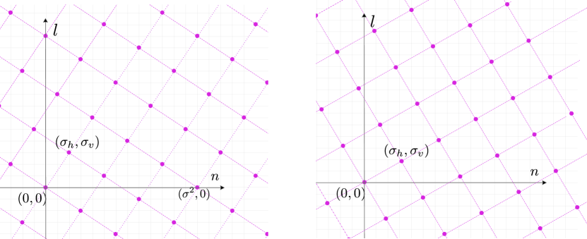
Figure 1: Both panels show the sublattice ${\mathbb{Z}^{2}_{\times}}$ obtained after the coordinate transformation (1.2), for the rational direction $(\sigma_{h},\sigma_{v})=(2,3)$ on the left and the irrational angle $\pi/6$ on the right. We see that the left lattice is a proper subset of $\mathbb{Z}^{2}$. On the right however the purple dots only coincide with $\mathbb{Z}^{2}$ at the origin. Moreover, the sets $\{i\sigma_{h}+j\sigma_{v}:(i,j)\in\mathbb{Z}^{2}\}$ and $\{i\sigma_{v}-j\sigma_{h}:(i,j)\in\mathbb{Z}^{2}\}$ are both dense in ${\mathbb{R}}$. This feature significantly differentiates the analysis between the rational and irrational directions.

For our purposes in this paper, the main consequence of the spatial discreteness is that it is no longer possible to construct sub- and super-solutions by applying relatively straightforward phase modulations to the profile $\Phi$ as in (1.14). Indeed, the shifts in (1.16) prevent us from simply factorizing out a common factor $\Phi^{\prime}(\xi)$ from the associated residuals as was possible in the series [33, 35, 6]. Inspired by normal form theory, we circumvent this problem by using a super-solution Ansatz of the form

$$u^{+}_{n,l}(t)=\Phi\big{(}n-\theta_{l}(t)+Z(t)\big{)}+\sum_{k=-N}^{N}p_{k}\big{(}n-\theta_{l}(t)+Z(t)\big{)}\big{(}\theta_{l+k}(t)-\theta_{l}(t)\big{)}\\ +\sum_{k=-N}^{N}\sum_{k^{\prime}=-N}^{N}q_{k,k^{\prime}}\big{(}n-\theta_{l}(t)+Z(t)\big{)}\big{(}\theta_{l+k}(t)-\theta_{l}(t)\big{)}\big{(}\theta_{l+k^{\prime}}(t)-\theta_{l}(t)\big{)}+z(t),$$ (1.17)

in which $N=2\max\{|\sigma_{h}|,|\sigma_{v}|\}$. The auxiliary functions $(p_{k})$, and $(q_{k,k^{\prime}})$ are chosen in such a way that the dangerous slowly decaying terms caused by the lattice anisotropy are cancelled. To achieve this, it is necessary to carefully analyze the spectral stability properties of the underlying planar wave $(c,\Phi)$ and exploit the Fredholm theory for linear MFDEs that was developed by Mallet-Paret [30].

The Ansatz (1.17) (but with different functions $p$, $q$ and $\theta$) first appeared in [17] - where it was used to study the evolution of initial conditions of the form

$$u_{i,j}(0)=\Phi\big{(}n(i,j)\big{)}+v^{0}_{i,j},\qquad\qquad\lim_{|i|+|j|\to\infty}|v^{0}_{i,j}|\to 0.$$ (1.18)

The authors established algebraic decay rates for the convergence

$$u_{ij}(t)\to\Phi(n(i,j)-ct),$$ (1.19)

hence establishing the stability of the planar wave (1.15) under localized perturbations, which form a (restrictive) subset of the general class (1.3) considered here.

The main novel aspect compared to [17] is that we need to incorporate nonlinear terms in the evolution of $\theta$ in order to capture the curvature-driven interface dynamics resulting from the non-local nature of the perturbations. Indeed, our evolution equation for $\theta$ takes the form

$$\dot{\theta}_{l}(t)=\dfrac{1}{d}\sum_{k=-N}^{N}a_{k}\left(e^{d(\theta_{l+k}(t)-\theta_{l}(t))}-1\right)+c,$$ (1.20)

for a set of coefficients $(a_{k})$ that is prescribed by the normal form analysis discussed above. For now, we simply mention that the parameter $d$ can be directly expressed in terms of important geometric and spectral quantities associated to the wave $(c,\Phi)$. As we discuss in the sequel, this will allow us to make the connection between (1.20) and a discretized mean curvature flow.

As in the continuous case, solutions to (1.20) can be used to approximate the behaviour of the phase $\gamma$ appearing in (1.4). This control is sufficiently strong to establish the convergence $\gamma(t)\to ct+\mu$ for initial conditions of the form

$$u_{i,j}(0)=\Phi\big{(}n(i,j)-\kappa_{l}\big{)}+v^{0}_{i,j},\qquad\qquad\lim_{|i|+|j|\to\infty}|v^{0}_{i,j}|\to 0,$$ (1.21)

where $\kappa_{l}$ is an arbitrary periodic sequence. The main significance compared to the earlier results in [16, 17] is that this corresponds to an ‘infinite-energy’ shift in the underlying wave position, during which the periodic wrinkles are flattened out under the flow of (1.20).

In our earlier work [23] we restricted attention to the horizontal direction $(\sigma_{h},\sigma_{v})=(1,0)$, which greatly simplified the analysis of (1.17) and (1.20). Indeed, we were able to choose $N=1$, with $a_{1}=a_{-1}=1$ and $p_{-1}=p_{1}=0$, which means that the linear terms reduce to the standard discrete heat equation. Solutions could hence be represented explicitly in terms of modified Bessel functions of the first kind, for which detailed bounds are available in the literature. In addition, the remaining auxiliary functions satisfied the useful identities

$$q_{-1,+1}=q_{+1,-1}=0,\qquad\qquad q_{-1,-1}=q_{+1,+1},$$ (1.22)

allowing the quadratic terms in the super-solution residual to be analyzed in a transparant fashion.

For general rational directions, some of the coefficients $a_{k}$ can become negative, in which case (1.20) no longer admits a comparison principle. In addition, we can no longer represent our solutions in terms of special functions for which powerful off-the-shelf estimates are available. We resolve these issues in §5-6 by developing an approximate comparison principle and using the saddle-point method to extract the necessary decay rates on the Green’s function for the linear part of (1.20).

Mean curvature flows

Matano and Nara proved in [34] that the solution $\theta(t)$ to the PDE (1.13) can be approximated by solutions $\Gamma$ to the PDE

$$\dfrac{\Gamma_{t}}{\sqrt{1+\Gamma_{y}^{2}}}=\dfrac{\Gamma_{yy}}{(1+\Gamma_{y}^{2})^{3/2}}+c.$$ (1.23)

This equation is known as a mean curvature flow equation with an additional drift term $c$. Indeed, writing $\nu(y,t)$ for the rightward-pointing normal vector of the interfacial graph $\{\Gamma(y,t),y)\}$, together with $V(y,t)$ for the horizontal velocity vector and $H(y,t)$ for the curvature, we can make the identifications

$$\nu=\big{[}1+\Gamma_{y}^{2}\big{]}^{-1/2}(1,-\Gamma_{y}),\qquad\qquad V=(\Gamma_{t},0\big{)},\qquad\qquad H=\big{[}1+\Gamma_{y}^{2}\big{]}^{-3/2}\Gamma_{yy}.$$ (1.24)

In particular, (1.23) can be written in the form

$$V\cdot\nu=H+c,$$ (1.25)

which reflects the rotational invariance of the wavespeed $c$.

In the discrete setting there is no ‘canonical’ notion of a mean curvature flow due to the absence of a suitable normal vector for the interface $(\Gamma_{l},l)$. Indeed, for a fixed index $l\in\mathbb{Z}$ one can consider the angle

$$\varphi_{l;k}(\Gamma)=\arctan{\dfrac{\Gamma_{l}-\Gamma_{l+k}}{k}},$$ (1.26)

for any $k\in\mathbb{Z}$, which measures the orientation of the vector that is transverse to the connection between $(\Gamma_{l},l)$ and $(\Gamma_{l+k},l+k)$; see Figure 2. These can all be considered as normal directions in some sense.

However, it is possible and natural to apply appropriate discretization schemes to (1.25). In order to take the lattice anisotropy into account, we start by writing $c_{\varphi}$ for the wavespeed associated to the planar wave solutions

$$u_{ij}(t)=\Phi_{\varphi}\big{(}n\cos\varphi+l\sin\varphi-c_{\varphi}t\big{)}$$ (1.27)

to (1.1) that travel at an additional angle of $\varphi$ relative to our original planar wave (1.15). This allows us to define the directional dispersion

$$\mathcal{D}(\varphi)=\dfrac{c_{\varphi}}{\cos\varphi},$$

which measures the speed at which level sets of the wave $(c_{\varphi},\Phi_{\varphi})$ move along the $n$-direction.

Setting out to discretize the terms in (1.25), we first introduce the average

$$[\overline{c}_{\Gamma}]_{l}=\dfrac{1}{2N}\sum_{0<|k|\leq N}c_{\varphi_{l;k}(\Gamma)},$$ (1.28)

where we use $2N$ neighbours in order to account for all the interactions present in (1.20). In addition, we introduce the notation

$$[\beta_{\Gamma}]_{l}=\sqrt{1+\sum_{0<|k|\leq N}\dfrac{A_{k}}{k^{2}}{(\Gamma_{l+k}-\Gamma_{l})^{2}}},\qquad\qquad[\Delta_{\Gamma}]_{l}=\sum_{0<|k|\leq N}\frac{2B_{k}}{k^{2}}(\theta_{l+k}-\theta_{l}),$$ (1.29)

which depends on two sequences $(A_{k})$ and $(B_{k})$. These must satisfy the normalization conditions

$$\sum_{0<|k|\leq N}A_{k}=1,\qquad\qquad\sum_{0<|k|\leq N}B_{k}=1,\qquad\qquad\sum_{0<|k|\leq N}B_{k}/k=0\qquad\qquad$$ (1.30)

in order to ensure that $\beta_{\Gamma}$ and $\Delta_{\Gamma}$ reduce formally to the symbols $\sqrt{1+\Gamma_{y}^{2}}$ and $\Gamma_{yy}$ in the continuum limit.

These sequences weigh the contributions of each of the normal directions $\varphi_{l;k}$ to the components of our discrete curvature flow, which we formulate as

$$\beta_{\Gamma}^{-1}\dot{\Gamma}=\kappa_{H}\beta_{\Gamma}^{-3}\Delta_{\Gamma}+\overline{c}_{\Gamma}.$$ (1.31)

It turns out that (1.31) and (1.20) can be matched up to cubic terms if and only if the parameters are chosen as

$$\kappa_{H}=\dfrac{1}{2}\sum_{k=-N}^{N}k^{2}a_{k},\qquad\qquad d=\frac{[\partial_{\varphi}^{2}\mathcal{D}(\varphi)]_{\varphi=0}}{2\kappa_{H}}.$$ (1.32)

The latter expression precisely matches the choice that comes from the technical considerations that lead to (1.20) during the construction of our super-solution (1.17). It also plays a key role in the related studies [15, 19] that concern travelling corner solutions in anisotropic media.

Outlook

In this paper we have restricted our attention to rational directions, primarily due to the fact that we lose the periodicity of the Fourier transform for irrational directions. In fact, the relevant Fourier symbol becomes quasi-periodic, making it very cumbersome to extract the necessary decay estimates. We are working on further reduction steps to bypass this issue, which could eventually allows us to consider general rounded interfaces. On the other hand, we do believe that the approach developed here is already strong enough to handle further questions such as the stability of the corner solutions constructed in [19] or the propagation of wavefronts through structured networks.

Organization

This paper is organized as follows. After stating our main results in §2, we discuss the asymptotic formation of interfaces in §3 and §4 by exploiting the properties of $\omega$-limit points. These sections simplify the ideas in [23] and adapt them to the more general setting considered in this paper. We proceed in §5 by studying the linearization of our phase LDE (1.20). In particular, we use techniques inspired by the saddle-point method to extract our required decay rates and establish a quasi-comparison principle. These are used in §6 to incorporate the nonlinear terms in (1.20) and build the bridge with the discrete curvature flow (1.31). These ingredients allow us to construct sub- and super-solutions for (1.1) in §7, which are subsequently used in §8 to establish our final stability results.

Acknowledgments

Both authors acknowledge support from the Netherlands Organization for Scientific Research (NWO) (grant 639.032.612).

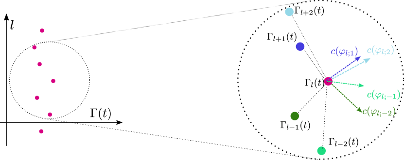
Figure 2: Here we provide the geometric motivation behind the definition (1.28) for $\overline{c}_{\Gamma}$ with $N=2$. Since there is no uniquely defined normal direction for discrete graphs, we take the average of the velocities associated to the directions transverse to the connecting lines between $(\Gamma_{l},l)$ and $(\Gamma_{l+k},l+k)$. Here we consider each $0<|k|\leq 2$.

2 Main results

In this paper we are interested in the discrete Allen-Cahn equation

$$\dot{u}_{i,j}(t)=[\Delta^{+}u(t)]_{i,j}+g\big{(}u_{i,j}(t)\big{)}$$ (2.1)

posed on the planar lattice $\mathbb{Z}^{2}$. The plus-shaped discrete Laplacian $\Delta^{+}:\ell^{\infty}(\mathbb{Z}^{2})\to\ell^{\infty}(\mathbb{Z}^{2})$ acts as a sum of differences over the nearest neighbors

$$\left[\Delta^{+}u\right]_{i,j}=u_{i+1,j}+u_{i,j+1}+u_{i-1,j}+u_{i,j-1}-4u_{i,j},$$ (2.2)

while the nonlinear function $g$ satisfies the following standard bistability condition.

• The nonlinearity $g:{\mathbb{R}}\to{\mathbb{R}}$ is $C^{3}$-smooth and there exists $a\in(0,1)$ such that

  $$g(0)=g(a)=g(1)=0,\qquad\qquad g^{\prime}(0)=g^{\prime}(1)<0.$$

  In addition, we have the inequalities

  $$g(x)>0\ \text{for}\ x\in(-\infty,0)\cup(a,1),\quad g(x)<0\ \text{for}\ x\in(0,a)\cup(1,\infty).$$

In this paper we focus on travelling waves propagating in rational directions. That is, we pick a direction $(\sigma_{h},\sigma_{v})\in\mathbb{Z}^{2}$ with $\mathrm{gcd}(\sigma_{h},\sigma_{v})=1$ and consider wave-profiles $\Phi_{*}$ that connect the two stable equilibria of the nonlinear function $g$, while traveling with the speed $c_{*}$ in the direction $(\sigma_{h},\sigma_{v})$.

It is convenient to pass to a new $(n,l)$-coordinate system that is oriented parallel $(n)$ and transverse $(l)$ to the direction of wave-propagation. In particular, we write

$$n=i\sigma_{h}+j\sigma_{v},\qquad\qquad l=i\sigma_{v}-j\sigma_{h}$$

and introduce the notation

$${\mathbb{Z}^{2}_{\times}} =\left\{(n,l)\in\mathbb{Z}^{2}:\exists(i,j)\in\mathbb{Z}^{2}:n=i\sigma_{h}+j\sigma_{v},\ l=i\sigma_{v}-j\sigma_{h}\right\}\subset\mathbb{Z}^{2}$$

for the image of the original grid $\mathbb{Z}^{2}$. Upon introducing the quantities

$$\sigma_{*}=\sqrt{\sigma_{h}^{2}+\sigma_{v}^{2}},\qquad\qquad\sigma_{\infty}=\max\{|\sigma_{h}|,|\sigma_{v}|\},$$ (2.3)

we point out the mappings

$$(i+\sigma_{h},j+\sigma_{v})\mapsto(n+\sigma_{*}^{2},l),\qquad\qquad(i+\sigma_{v},j-\sigma_{h})\mapsto(n,l+\sigma_{*}^{2}),$$ (2.4)

which implies that for any $(n,l)\in{\mathbb{Z}^{2}_{\times}}$ the point $(n+a\sigma_{*}^{2},l+b\sigma_{*}^{2})$ is also an element of ${\mathbb{Z}^{2}_{\times}}$ for any $(a,b)\in\mathbb{Z}^{2}$, see Figure 1.

In this new coordinate system the discrete Laplace operator (2.2) transforms as

$$[\Delta^{\times}u]_{n,l}=u_{n+\sigma_{h},l+\sigma_{v}}+u_{n+\sigma_{v},l-\sigma_{h}}+u_{n-\sigma_{h},l-\sigma_{v}}+u_{n-\sigma_{v},l+\sigma_{h}}-4u_{n,l}.$$ (2.5)

In particular, the initial value problem that we consider in this paper can be written in the form

$$\dot{u}_{n,l}(t) =[\Delta^{\times}u(t)]_{n,l}+g\big{(}u_{n,l}(t)\big{)},\qquad(n,l)\in{{\mathbb{Z}^{2}_{\times}}},\qquad t>0,$$ (2.6)

$$u_{n,l}(0) =u_{n,l}^{0},$$ (2.7)

for some initial condition $u^{0}\in\ell^{\infty}(\mathbb{Z}^{2}_{\times})$. Our second assumption imposes a ‘front-like’ property on this initial condition $u^{0}$.

• The initial condition $u^{0}\in\ell^{\infty}({\mathbb{Z}^{2}_{\times}})$ satisfies

  $$\limsup_{n\to-\infty}\sup_{l\in\mathbb{Z}:(n,l)\in{\mathbb{Z}^{2}_{\times}}}u^{0}_{n,l}<a,\qquad\qquad\liminf_{n\to+\infty}\inf_{l\in\mathbb{Z}:(n,l)\in{\mathbb{Z}^{2}_{\times}}}u^{0}_{n,l}>a.$$ (2.8)

2.1 Travelling waves

A travelling wave solution is any solution of the form

$$u_{n,l}(t)=\Phi_{*}(n-c_{*}t)$$ (2.9)

for some wave-profile $\Phi_{*}$ and speed $c_{*}\in{\mathbb{R}}$. Any such pair must necessarily satisfy the MFDE

$$-c_{*}\Phi_{*}^{\prime}(\xi)=\Phi_{*}(\xi+\sigma_{h})+\Phi_{*}(\xi+\sigma_{v})+\Phi_{*}(\xi-\sigma_{h})+\Phi_{*}(\xi-\sigma_{v})-4\Phi_{*}(\xi)+g\big{(}\Phi_{*}(\xi)\big{)},$$ (2.10)

which we augment with the boundary conditions

$$\lim_{\xi\to-\infty}\Phi_{*}(\xi)=0,\qquad\lim_{\xi\to\infty}\Phi_{*}(\xi)=1.$$ (2.11)

The existence of such pairs $(c_{*},\Phi_{*})$ was established by Mallet-Paret in [31], both for rational and irrational directions. The wave-speed $c_{*}$ is unique once the direction $(\sigma_{h},\sigma_{v})$ and the detuning parameter $a$ have been fixed, while the wave-profile $\Phi_{*}$ is monotonically increasing and unique up to translations provided that $c_{*}\neq 0$. In contrast to the continuous setting, there can be a range of values for $a$ where $c_{*}=0$ holds; see [19] for a detailed discussion. The assumption below ensures that we are outside of this so-called pinning regime.

• There exists a wave-speed $c_{*}\neq 0$ and a monotone wave profile $\Phi_{*}$ that satisfy the MFDE (2.10) together with the boundary conditions (2.11) and the phase normalization $\Phi_{*}(0)=\frac{1}{2}$.

To examine the stability properties of the wave-pair $(\Phi_{*},c_{*})$ under the dynamics of (2.6), one usually starts by considering the linear variational problem

$$\dot{v}_{n,l}(t)=[\Delta^{\times}v(t)]_{n,l}+g^{\prime}\big{(}\Phi_{*}(n-c_{*}t)\big{)}v_{n,l}(t).$$

Taking the discrete Fourier transform along the transverse direction $l$, the problem decouples into the set of one-dimensional LDEs

$$\dot{v}_{n}(t) =e^{i\omega\sigma_{v}}v_{n+\sigma_{h}}(t)+e^{-i\omega\sigma_{h}}v_{n+\sigma_{v}}(t)+e^{-i\omega\sigma_{v}}v_{n-\sigma_{h}}(t)+e^{i\omega\sigma_{h}}v_{n-\sigma_{v}}(t)-4v_{n}(t)$$ (2.12)

$$\qquad+g^{\prime}\big{(}\Phi_{*}(n-c_{*}t)\big{)}v_{n}(t),$$

indexed by the frequency variable $\omega\in[-\pi,\pi]$. As shown in [21, §2], there is a close relationship between the Green’s function for each of the LDEs (2.12) and their associated linear operators

$$\mathcal{L}_{\omega}:W^{1,\infty}({\mathbb{R}};{\mathbb{C}})\to L^{\infty}({\mathbb{R}};{\mathbb{C}}),\qquad\omega\in[-\pi,\pi]$$

which act as

$$\left[\mathcal{L}_{\omega}p\right](\xi) =c_{*}p^{\prime}(\xi)+e^{i\omega\sigma_{v}}p(\xi+\sigma_{h})+e^{-i\omega\sigma_{h}}p(\xi+\sigma_{v})+e^{-i\omega\sigma_{v}}p(\xi-\sigma_{h})+e^{i\omega\sigma_{h}}p(\xi-\sigma_{v})$$ (2.13)

$$\qquad-4p(\xi)+g^{\prime}\big{(}\Phi_{*}(\xi)\big{)}p(\xi).$$

A special role is reserved for the operator $\mathcal{L}_{0}$, which encodes the linearized behaviour of the wave $\Phi_{*}$ under perturbations that are homogeneous in the transverse direction. We briefly summarize several key Fredholm properties of this operator that were obtained by Mallet-Paret in the classic paper [30].

Lemma 2.1 (see [30]).

Assume that (Hg) and $(H\Phi)$ are satisfied. Then the operator $\mathcal{L}_{0}:W^{1,\infty}({\mathbb{R}};{\mathbb{C}})\to L^{\infty}({\mathbb{R}};{\mathbb{C}})$ is Fredholm with index zero. It has a one-dimensional kernel spanned by the strictly positive function $\Phi_{*}^{\prime}$. In addition, its range admits the characterization

$$\mathcal{R}(\mathcal{L}_{0})=\left\{f\in L^{\infty}({\mathbb{R}};{\mathbb{R}}):\int_{\mathbb{R}}\psi_{*}(\xi)f(\xi)\,d\xi=0\right\}$$ (2.14)

for some strictly positive bounded function $\psi_{*}\in C^{2}({\mathbb{R}};{\mathbb{R}})$ that we normalize to have

$$\int_{\mathbb{R}}\psi_{*}(\xi)\Phi_{*}^{\prime}(\xi)d\xi=1.$$ (2.15)

Since clearly $\Phi_{*}^{\prime}\notin\mathcal{R}(\mathcal{L}_{0})$ we see that $\lambda=0$ is a simple eigenvalue of the operator $\mathcal{L}_{0}$. The following result states that this property extends to a branch of simple eigenvalues $\lambda_{\omega}$ for the operators $\mathcal{L}_{\omega}$ with $\omega\approx 0$.

Lemma 2.2 (see [16, Prop. 2.2]).

Assume that (H$g$) and (H$\Phi$) are satisfied. Then there exists a constant $0<\omega_{0}\ll 1$ together with pairs

$$(\lambda_{\omega},\phi_{\omega})\in{\mathbb{C}}\times W^{1,\infty}({\mathbb{R}};{\mathbb{C}}),$$

defined for each $\omega\in(-\omega_{0},\omega_{0})$, that satisfy the following properties.

1. For each $\omega\in(-\omega_{0},\omega_{0})$ we have the characterization

   $$\mathrm{Ker}(\mathcal{L}_{\omega}-\lambda_{\omega})=\mathrm{span}\left\{\phi_{\omega}\right\},$$

   together with the algebraic simplicity condition

   $$\phi_{\omega}\notin\mathcal{R}(\mathcal{L}_{\omega}-\lambda_{\omega}).$$

2. We have $\lambda_{0}=0$, $\phi_{0}=\Phi_{*}^{\prime}$ and the maps $\omega\mapsto\lambda_{\omega}$, $\omega\mapsto\phi_{\omega}$ are analytic.

3. For each $\omega\in(-\omega_{0},\omega_{0})$ we have the normalization

   $$\langle\phi_{\omega},\psi_{*}\rangle_{L^{2}}=1.$$

Our following assumption states that the map $\omega\mapsto\lambda_{\omega}$ touches the origin in a quadratic tangency, opening up to the left of the imaginary axis. This is a rather standard condition that was also used in [16] and [17] to show that transverse phase deformations decay at the standard rates prescribed by the heat equation. We remark that Lemma 6.3 in [16] guarantees that this condition is satisfied whenever the propagation direction is close to horizontal or diagonal. Furthermore, numerical experiments in [16, §6] suggest that this extends to all directions where the wavespeed does not vanish.

• The branch of eigenvalues $(\lambda_{\omega})_{\omega\approx 0}$ satisfies the inequality

  $$[\partial_{\omega}^{2}\lambda_{\omega}]_{\omega=0}<0.$$

Our final spectral assumption is far less standard and requires some technical preparations. To this end, we introduce the set of shifts

$$(\tau_{1},\tau_{2},\tau_{3},\tau_{4})=(\sigma_{h},\sigma_{v},-\sigma_{h},-\sigma_{v})$$ (2.16)

and their associated translation operators $T_{\nu}$ that act as

$$[T_{\nu}h](\xi)=h(\xi+\tau_{\nu}),\qquad\nu\in\left\{1,2,3,4\right\}$$ (2.17)

for any function $h\in C({\mathbb{R}})$. These can be used to define a collection of functions $p^{\diamond}$, $p^{\diamond\diamond}$ and $q^{\diamond\diamond}$ that play a key role in §7 where we construct sub- and super-solutions for (2.6). For our purposes here, we are chiefly interested in the associated coefficients $\alpha^{\diamond}_{p}$, $\alpha^{\diamond\diamond}_{p}$ and $\alpha^{\diamond\diamond}_{q}$ that are related to the solvability condition (2.14).

Lemma 2.3 (see §6).

Assume that $(Hg)$ and $(H\Phi)$ both hold. Then for every $\nu,\nu^{\prime}\in\left\{1,2,3,4\right\}$ there exist bounded functions

$$p_{\nu}^{\diamond},p_{\nu\nu^{\prime}}^{\diamond\diamond},q_{\nu\nu^{\prime}}^{\diamond\diamond}:{\mathbb{R}}\to{\mathbb{R}}$$

that satisfy the identities

$$\begin{array}[]{lcl}\left[\mathcal{L}_{0}p^{\diamond}_{\nu}\right](\xi)&=&[T_{\nu}\Phi^{\prime}](\xi)-\alpha^{\diamond}_{p;\nu}\Phi^{\prime}(\xi),\\[8.5359pt] [\mathcal{L}_{0}p^{\diamond\diamond}_{\nu\nu^{\prime}}](\xi)&=&\alpha_{p;\nu^{\prime}}^{\diamond}p^{\diamond}_{\nu}(\xi)-[T_{\nu^{\prime}}p_{\nu}^{\diamond}](\xi)-\alpha^{\diamond\diamond}_{p;\nu\nu^{\prime}}\Phi^{\prime}(\xi),\\[8.5359pt] [\mathcal{L}_{0}q^{\diamond\diamond}_{\nu\nu^{\prime}}](\xi)&=&-\alpha_{p;\nu}^{\diamond}\dfrac{d}{d\xi}p_{\nu}^{\diamond}(\xi)+[T_{\nu^{\prime}}\dfrac{d}{d\xi}p_{\nu}^{\diamond}](\xi)-\dfrac{1}{2}g^{\prime\prime}\big{(}\Phi_{*}(\xi)\big{)}p_{\nu}^{\diamond}(\xi)p_{\nu^{\prime}}^{\diamond}(\xi)\\ &&\qquad-\dfrac{1}{2}\mathbf{1}_{\nu=\nu^{\prime}}[T_{\nu}\Phi_{*}^{\prime\prime}](\xi)-\alpha^{\diamond\diamond}_{q;\nu\nu^{\prime}}\Phi^{\prime}(\xi).\\ \end{array}$$ (2.18)

Here the coefficients $\alpha_{p;\nu}^{\diamond}$, $\alpha_{p;\nu\nu^{\prime}}^{\diamond\diamond}$ and $\alpha_{q;\nu\nu^{\prime}}^{\diamond\diamond}$ are given by

$$\begin{array}[]{lcl}\alpha_{p;\nu}^{\diamond}&=&\int_{\mathbb{R}}[T_{\nu}\Phi^{\prime}](\xi)\psi_{*}(\xi)d\xi,\\[8.5359pt] \alpha^{\diamond\diamond}_{p;\nu\nu^{\prime}}&=&\int_{\mathbb{R}}\left[\alpha_{p;\nu}^{\diamond}p^{\diamond}_{\nu^{\prime}}(\xi)-[T_{\nu^{\prime}}p_{\nu}^{\diamond}](\xi)\right]\psi_{*}(\xi)d\xi,\\[8.5359pt] \alpha^{\diamond\diamond}_{q;\nu\nu^{\prime}}&=&\int_{{\mathbb{R}}}\left(-\alpha_{p;\nu}^{\diamond}\dfrac{d}{d\xi}p_{\nu^{\prime}}^{\diamond}(\xi)+[T_{\nu^{\prime}}\dfrac{d}{d\xi}p_{\nu}^{\diamond}](\xi)-\dfrac{1}{2}g^{\prime\prime}\big{(}\Phi_{*}(\xi)\big{)}p_{\nu}^{\diamond}(\xi)p_{\nu^{\prime}}^{\diamond}(\xi)\right)\psi_{*}(\xi)d\xi\\ &&\qquad-\dfrac{1}{2}\int_{{\mathbb{R}}}\mathbf{1}_{\nu=\nu^{\prime}}[T_{\nu}\Phi_{*}^{\prime\prime}](\xi)\psi_{*}(\xi)d\xi.\\ \end{array}$$ (2.19)

Moreover, the functions $p^{\diamond}_{\nu},p^{\diamond\diamond}_{\nu\nu^{\prime}}$ and $q^{\diamond\diamond}_{\nu\nu^{\prime}}$ can be chosen in such a way that

$$\langle p^{\diamond}_{\nu},\psi_{*}\rangle_{L^{2}}=0,\qquad\langle p^{\diamond\diamond}_{\nu\nu^{\prime}},\psi_{*}\rangle_{L^{2}}=0,\qquad\langle q^{\diamond\diamond}_{\nu\nu^{\prime}},\psi_{*}\rangle_{L^{2}}=0.$$ (2.20)

Upon introducing the convenient notation

$$(\sigma_{1},\sigma_{2},\sigma_{3},\sigma_{4})=(\sigma_{v},-\sigma_{h},-\sigma_{v},\sigma_{h}),$$ (2.21)

we now use the coefficients (2.19) to introduce the function $f_{(\sigma_{h},\sigma_{v})}:[-\pi,\pi]\to{\mathbb{R}}$ that acts as

$$\begin{array}[]{lcl}f_{(\sigma_{h},\sigma_{v})}(\omega)&=&\sum_{\nu=1}^{4}\alpha_{p;\nu}^{\diamond}(\cos{(\sigma_{\nu}\omega)}-1)\\[5.69046pt] &&\qquad+\sum_{\nu,\nu^{\prime}=1}^{4}\alpha_{p;\nu\nu^{\prime}}^{\diamond\diamond}\Big{(}\cos{\big{(}(\sigma_{\nu}+\sigma_{\nu^{\prime}})\omega\big{)}}-\cos{(\sigma_{\nu}\omega)}-\cos{(\sigma_{\nu^{\prime}}\omega)}+1\Big{)}.\end{array}$$ (2.22)

For the sequel, it is convenient to rewrite this expression in a more compact form. To this end, we write $N=\max_{\nu,\nu^{\prime}\in\{1,2,3,4\}}\left\{\sigma_{\nu},\sigma_{\nu}+\sigma_{\nu^{\prime}}\right\}$ and introduce the sequence

$$a_{k}=\sum_{\nu=1}^{4}\alpha_{p;\nu}^{\diamond}\textbf{1}_{\{k=\sigma_{\nu}\}}+\sum_{\nu,\nu^{\prime}=1}^{4}\alpha_{p;\nu\nu^{\prime}}^{\diamond\diamond}\big{(}\textbf{1}_{\{k=\sigma_{\nu}+\sigma_{\nu^{\prime}}\}}-\textbf{1}_{\{k=\sigma_{\nu}\}}-\textbf{1}_{\{k=\sigma_{\nu^{\prime}}\}}\big{)},$$ (2.23)

which allows us to rewrite (2.22) as

$$f_{(\sigma_{h},\sigma_{v})}(\omega)=\sum_{k=-N}^{N}a_{k}(\cos{(k\omega)}-1).$$ (2.24)

This function will appear later as the real part of the Fourier symbol associated to the linear dynamics of the transverse phase of the planar wave $(c_{*},\Phi_{*})$.

In the horizontal case $(\sigma_{h},\sigma_{v})=(1,0)$ we can take $N=1$, $a_{-1}=1$, $a_{1}=1$ and

$$f_{(1,0)}(\omega)=2(\cos\omega-1),$$ (2.25)

but in general the coefficients $a_{k}$ can be negative. In order to ensure that our phase dynamics can be controlled, our final assumption requires the function $f$ to be strictly negative for all non-zero $\omega$.

• The inequality $f_{(\sigma_{h},\sigma_{v})}(\omega)<0$ holds for all $\omega\in[-\pi,\pi]\backslash\{0\}$.

We now set out to obtain some geometric intuition concerning the coefficients (2.18) and the Fourier symbol (2.24). We first note that the pair $(c_{*},\Phi_{*})$ can be perturbed in order to yield waves travelling in directions that are ‘close’ to $(\sigma_{h},\sigma_{v})$. In particular, we follow the approach from [19] and look for solutions to the Allen-Cahn equation (2.6) of the form

$$u_{n,l}(t)=\Phi_{\varphi}(n\cos{\varphi}+l\sin{\varphi}-c_{\varphi}t),$$ (2.26)

which travel at an angle $\varphi$ through the rotated lattice $\mathbb{Z}^{2}_{\times}$. Inserting this Ansatz into (2.6), we find that the pair $(c_{\varphi},\Phi_{\varphi})$ must satisfy the MFDE

$$-c_{\varphi}\Phi_{\varphi}^{\prime}(\xi) =\Phi_{\varphi}(\xi+\sigma_{h}\cos{\varphi}+\sigma_{v}\sin{\varphi})+\Phi_{\varphi}(\xi+\sigma_{v}\cos{\varphi}-\sigma_{h}\sin{\varphi})$$ (2.27)

$$\qquad+\Phi_{\varphi}(\xi-\sigma_{h}\cos{\varphi}-\sigma_{v}\sin{\varphi})+\Phi_{\varphi}(\xi-\sigma_{v}\cos{\varphi}+\sigma_{h}\sin{\varphi})$$

$$\qquad-4\Phi_{\varphi}(\xi)+g\big{(}\Phi_{\varphi}(\xi)\big{)}.$$

Using standard bifurcation arguments one can show that the pair $(\Phi_{*},c_{*})$ can be embedded into a smooth branch of waves $(c_{\varphi},\Phi_{\varphi})$ for $\varphi\approx 0$.

Lemma 2.4 (see [19, Prop. 2.2] and [16, Thm. 2.7]).

Assume that (H$g$) and (H$\Phi$) are satisfied. Then there exists a constant $\delta_{\varphi}>0$ together with pairs

$$(c_{\varphi},\Phi_{\varphi})\in{\mathbb{R}}\times W^{1,\infty}({\mathbb{R}};{\mathbb{R}}),$$

defined for every $\varphi\in(-\delta_{\varphi},\delta_{\varphi})$, such that the following holds true.

1. For every $\varphi\in(-\delta_{\varphi},\delta_{\varphi})$ the pair $(c_{\varphi},\Phi_{\varphi})$ satisfies the MFDE (2.27) together with the boundary conditions (2.11).

2. For every $\varphi\in(-\delta_{\varphi},\delta_{\varphi})$ we have the normalization $\langle\Phi_{\varphi}-\Phi_{*},\psi_{*}\rangle=0$.

3. The maps $\varphi\mapsto c_{\varphi}$ and $\varphi\mapsto\Phi_{\varphi}$ are $C^{2}$-smooth, with $(c_{0},\Phi_{0})=(c_{*},\Phi_{*})$.

Our next result shows that there is a close link between the coefficients (2.18), the pairs $(\lambda_{\omega},\phi_{\omega})$ constructed in Lemma 2.3 and the waves $(c_{\varphi},\Phi_{\varphi})$ described in Lemma 2.4. These identities can be stated in a compact fashion by virtue of the choices (2.16) and (2.21).

Lemma 2.5 (see §6).

Assume that (H$g$) and (H$\Phi$) are satisfied. Then the following identities hold.

1. $c_{*}=-\sum_{\nu=1}^{4}\tau_{\nu}\alpha_{p;\nu}^{\diamond}$,

2. $[\partial_{\varphi}c_{\varphi}]_{\varphi=0}=-\sum_{\nu=1}^{4}\sigma_{\nu}\alpha_{p;\nu}^{\diamond}=-\sum_{k=-N}^{N}a_{k}k$,

3. $[\partial^{2}_{\varphi}c_{\varphi}]_{\varphi=0}=-c_{*}+2\sum_{\nu=1}^{4}\sum_{\nu^{\prime}=1}^{4}\sigma_{\nu}\sigma_{\nu^{\prime}}\alpha_{q;\nu\nu^{\prime}}^{\diamond\diamond}$,

4. $[\partial_{\varphi}\Phi_{\varphi}]_{\varphi=0}=-\sum_{\nu=1}^{4}\sigma_{\nu}p_{\nu}^{\diamond}$,

5. $[\partial_{\omega}\lambda_{\omega}]_{\omega=0}=\sum_{\nu=1}^{4}\sigma_{\nu}\alpha_{p;\nu}^{\diamond}$,

6. $[\partial_{\omega}^{2}\lambda_{\omega}]_{\omega=0}=-\sum_{\nu=1}^{4}\alpha_{\nu}^{\diamond}\sigma_{\nu}^{2}-\sum_{\nu,\nu^{\prime}=1}^{4}2\alpha_{p;{\nu\nu^{\prime}}}^{\diamond\diamond}\sigma_{\nu}\sigma_{\nu^{\prime}}=-\sum_{k=-N}^{N}a_{k}k^{2}$.

Combining item (vi) and (2.22), we readily see that

$$f^{\prime\prime}_{(\sigma_{h},\sigma_{v})}(0)=[\partial_{\omega}^{2}\lambda_{\omega}]_{\omega=0}.$$

This identity in combination with (HS$)_{1}$ implies that the function $f_{(\sigma_{h},\sigma_{v})}$ looks like a downwards parabola locally around $\omega=0$. This information was sufficient to obtain the ‘localized’ stability results in [16] and [17], but our more general setup here requires global information on the function $f_{(\sigma_{h},\sigma_{v})}$. An important role is reserved for the parameter

$$d=-\dfrac{\partial^{2}_{\varphi}[c_{\varphi}/\cos\varphi]_{\varphi=0}}{[\partial_{\omega}^{2}\lambda_{\omega}]_{\omega=0}}=-\dfrac{c_{*}+[\partial_{\varphi}^{2}c_{\varphi}]_{\varphi=0}}{[\partial_{\omega}^{2}\lambda_{\omega}]_{\omega=0}}=\dfrac{2\sum_{\nu=1}^{4}\sum_{\nu^{\prime}=1}^{4}\sigma_{\nu}\sigma_{\nu^{\prime}}\alpha_{q;\nu\nu^{\prime}}^{\diamond\diamond}}{\sum_{\nu=1}^{4}\alpha_{\nu}^{\diamond}\sigma_{\nu}^{2}+\sum_{\nu,\nu^{\prime}=1}^{4}2\alpha_{p;{\nu\nu^{\prime}}}^{\diamond\diamond}\sigma_{\nu}\sigma_{\nu^{\prime}}},$$ (2.28)

which is well-defined on account of assumption (HS$)_{1}$. It measures the ratio between the quadratic terms in the directional dispersion $c_{\varphi}/\cos\varphi$ and the branch of eigenvalues $\lambda_{\omega}$. This parameter also played a crucial role throughout the construction of travelling corners for (2.1); see [19, Eqs. (7.38) and (7.76)] where it appears as the quadratic coefficient on the center manifold that governs the transverse dynamics.

2.2 Interface formation

In this subsection we provide a construction for the set of phases $\big{(}\gamma_{l}(t)\big{)}_{l\in\mathbb{Z}}$ that should be seen as an approximation for the level set $u=\frac{1}{2}$. Indeed, due to the discreteness of the lattice one cannot necessarily find integers $n_{*}(l,t)$ for which $u_{n_{*}(l,t),l}(t)=\frac{1}{2}$ holds exactly - even when restricted to large times $t\gg 1$. Instead, we establish the following monotonicity result, which for fixed $l$ and large $t\gg 1$ allows us to capture the ‘crossing’ of $u$ through $\frac{1}{2}$ between $n=n_{*}(l,t)$ and $n=n_{*}(l,t)+\sigma_{*}^{2}$.

Proposition 2.6 (see $\S$4).

Suppose that (H$g$), (H$\Phi$) and (H$0$) are satisfied. There exists a time $T>0$ such that for every $l\in\mathbb{Z}$ and $t\geq T$ there exists a unique $n_{*}=n_{*}(l,t)$ with the property

$$0<u_{n_{*},l}(t)\leq\dfrac{1}{2},\qquad\qquad u_{n_{*}+\sigma_{*}^{2},l}(t)>\dfrac{1}{2}.$$ (2.29)

We now set out use an interpolation argument to construct $\gamma_{l}(t)$ from the quantities in (2.29). The main consideration is that for exact travelling waves $u_{n,l}(t)=\Phi_{*}(n-c_{*}t+\mu)$ we wish to recover the standard phase $\gamma_{l}(t)=c_{*}t-\mu$, in view of the fact that $\Phi_{*}(0)=\frac{1}{2}$. To achieve this, we define the phases

$$\theta_{l}^{-}(t)=\Phi_{*}^{-1}\big{(}u_{n_{*}(l,t),l}(t)\big{)},\qquad\qquad\theta_{l}^{+}(t)=\Phi_{*}^{-1}\big{(}u_{n_{*}(l,t)+\sigma_{*}^{2},l}(t)\big{)}$$ (2.30)

associated to the two values (2.29). Upon writing

$$\vartheta_{*}(l,t)=-\sigma_{*}^{2}\theta_{l}^{-}(t)/[\theta_{l}^{+}(t)-\theta_{l}^{-}(t)],$$ (2.31)

we note that the linear interpolation

$$\theta_{\mathrm{lin};l,t}(\xi)=\sigma_{*}^{-2}\theta_{l}^{+}(t)\xi-\sigma_{*}^{-2}\theta_{l}^{-}(t)(\xi-\sigma_{*}^{2})$$ (2.32)

satisfies

$$\theta_{\mathrm{lin};l,t}(0)=\theta_{l}^{-}(t),\qquad\qquad\theta_{\mathrm{lin};l,t}\big{(}\vartheta_{*}(l,t)\big{)}=0,\qquad\qquad\theta_{\mathrm{lin};l,t}(\sigma_{*}^{2})=\theta_{l}^{+}(t).$$ (2.33)

This motivates the phase-interpolated definition

$$\gamma_{l}(t)=n_{*}(l,t)+\vartheta_{*}(l,t),$$ (2.34)

which ensures that the ‘stretched’ profile $\tilde{\Phi}(\xi)=\Phi_{*}\Big{(}\theta_{\mathrm{lin};l,t}\big{(}\xi-n_{*}(l,t)\big{)}\Big{)}$ satisfies

$$\tilde{\Phi}\big{(}n_{*}(l,t)\big{)}=u_{n_{*}(l,t),l}(t),\qquad\qquad\tilde{\Phi}\big{(}\gamma_{l}(t)\big{)}=\frac{1}{2},\qquad\qquad\tilde{\Phi}\big{(}n_{*}(l,t)+\sigma_{*}^{2}\big{)}=u_{n_{*}(l,t)+\sigma_{*}^{2},l}(t).$$ (2.35)

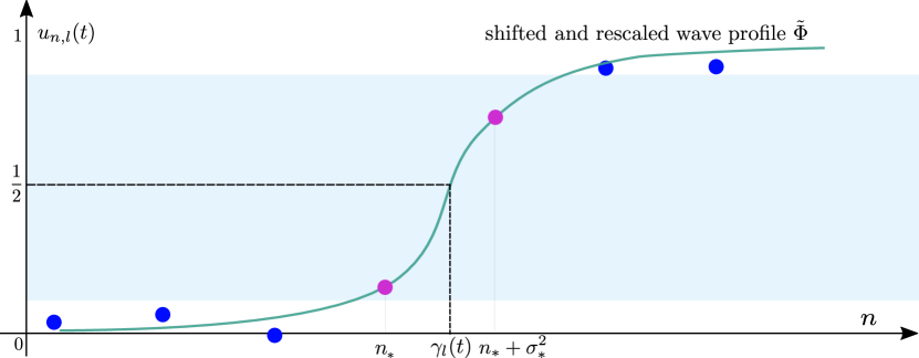
Figure 3: In order to construct the phase $\gamma_{l}(t)$ for a fixed pair $(l,t)$ we first identify an interfacial region around the value $\Phi_{*}(0)=\frac{1}{2}$ (shaded in blue) where the (discrete) function $n\mapsto u_{n,l}(t)$ is monotone. We subsequently stretch the waveprofile to match the (pink) points $\left(n_{*},u_{n_{*},l}(t)\right)$ and $\left(n_{*}+\sigma_{*}^{2},u_{n_{*}+\sigma_{*}^{2},l}(t)\right)$ introduced in (2.29).

Notice indeed that for the special case $u_{n,l}(t)=\Phi_{*}(n-c_{*}t+\mu)$ we have

$$\theta_{l}^{-}(t)=n_{*}(l,t)-c_{*}t+\mu,\qquad\qquad\theta_{l}^{+}(t)=n_{*}(l,t)+\sigma_{*}^{2}-c_{*}t+\mu,$$ (2.36)

which gives $\vartheta_{*}(l,t)=-\theta_{l}^{-}(t)$ and hence $\gamma_{l}(t)=c_{*}t-\mu$, as we desired.

The result below states that our phase indeed tracks the behaviour of $u$ in an asymptotic sense. We emphasize that there are several other choices for the phase that lead to similar results. For example, our previous construction in [23] did not stretch the wave and merely aligned it with $u$ at the point $n_{*}(l,t)$. Our more refined approach here allows us to streamline our arguments and avoid the discontinuities in $\gamma_{l}(t)$ that complicated our previous analysis at times.

Proposition 2.7 (see $\S$4).

Suppose that (H$g$), (H$\Phi$) and (H$0$) are satisfied. Then we have the limit

$$\lim_{t\to\infty}\sup_{(n,l)\in{\mathbb{Z}^{2}_{\times}}}|u_{n,l}(t)-\Phi_{*}\big{(}n-\gamma_{l}(t)\big{)}|=0.$$ (2.37)

2.3 Interface asymptotics

We are now ready to discuss the main technical results of this paper. These concern the asymptotic behaviour of the phase $\gamma(t)$ that we introduced in (2.34), which can be approximated by solutions to the scalar nonlinear LDE

$$\dot{\theta}(t)=\Theta_{\mathrm{ch}}\big{(}\theta(t)\big{)}.$$ (2.38)

Here the function $\Theta_{\mathrm{ch}}:\ell^{\infty}(\mathbb{Z})\to\ell^{\infty}(\mathbb{Z})$ acts as

$$[\Theta_{\mathrm{ch}}(\theta)]_{l}=\begin{cases}\dfrac{1}{d}\sum_{k=-N}^{N}a_{k}\left(e^{d\big{(}\theta_{l+k}(t)-\theta_{l}(t)\big{)}}-1\right)+c_{*},&\quad d\neq 0,\\[8.5359pt] \sum_{k=-N}^{N}a_{k}\big{(}\theta_{l+k}(t)-\theta_{l}(t)\big{)}+c_{*},&\quad d=0,\end{cases}$$ (2.39)

where we have recalled the coefficients $(a_{k})$ and parameter $d$ that were introduced in (2.23) respectively (2.28). The label ‘ch’ refers to the fact that a Cole-Hopf transformation can be used to recast the nonlinear system for $d\neq 0$ into the linear system prescribed for $d=0$. This reduction is essential for our analysis in §6, where we obtain decay rates for solutions to (2.38), based on the linear theory that we develop in §5.

The decision to use (2.39) is hence primarily based on technical considerations. Nevertheless, it is possible to build a bridge back to the discrete curvature flow (1.31). To this end, we recall the definitions (1.28) and (1.29) and introduce the operator $\Theta_{\mathrm{dmc}}:\ell^{\infty}(\mathbb{Z})\mapsto\ell^{\infty}(\mathbb{Z})$ that acts as

$$\Theta_{\mathrm{dmc}}(\theta)=\kappa_{H}\frac{\Delta_{\theta}}{\beta_{\theta}^{2}}+\beta_{\theta}\overline{c}_{\theta},$$ (2.40)

which depends on the sequences (1.30) and the curvature coefficient $\kappa_{H}>0$.

The result below shows that $\Theta_{\mathrm{dmc}}$ can be tailored to agree with $\Theta_{\mathrm{ch}}$ up to terms that are cubic in the first-differences

$$[\partial\theta]_{l}=\theta_{l+1}-\theta_{l}.$$

We will see in §6 that such terms decay at a rate of $O(t^{-3/2})$, which in theory is sufficiently fast to be absorbed by our error terms. However, due to the loss of the comparison principle we did not attempt to compare the actual solutions to the respective LDEs as was possible in [23, Prop. 8.2].

Proposition 2.8 (see $\S$6).

Assume that (H$g$), (H$\Phi$), (H0), (HS$)_{1}$, (HS$)_{2}$ all hold. Assume furthermore that $\kappa_{H}=-{[\partial^{2}_{\omega}\lambda_{\omega}]_{\omega=0}}/{2}$. Then there exists a unique set of coefficients $(A_{k},B_{k})_{k=-N}^{N}$ that satisfy the identities (1.30) and allow us to find a constant $K>0$ for which

$$\left|\left|{\Theta_{\mathrm{ch}}(\theta)-\Theta_{\mathrm{dmc}}(\theta)}\right|\right|_{\ell^{\infty}}\leq K\left|\left|{\partial\theta}\right|\right|^{3}_{\ell^{\infty}}$$ (2.41)

holds for all sequences $\theta\in\ell^{\infty}(\mathbb{Z})$ with $\left|\left|{\partial\theta}\right|\right|_{\ell^{\infty}}\leq 1$. On the other hand, such coefficients do not exist if (1.32) is violated.

Our main result below makes the asymptotic connection between $\gamma$ and solutions $\theta$ to (2.38) fully precise. This allows us to gain detailed control over the long-term dynamics of the phase $\gamma(t)$, which can be used to provide stability results outside the ‘local’ regimes treated in [16] and [17].

Theorem 2.9 (see §8).

Assume that (H$g$), (H$\Phi$), (H0), (HS$)_{1}$, (HS$)_{2}$ all hold and let $u$ be a solution of (2.6) with the initial condition (2.7). Then for every $\epsilon>0$, there exists a constant $\tau_{\epsilon}>0$ so that for any $\tau\geq\tau_{\epsilon}$, the solution $\theta$ of LDE (2.38) with the initial value $\theta(0)=\gamma(\tau)$ satisfies

$$\left|\left|{\gamma(t)-\theta(t-\tau)}\right|\right|_{\ell^{\infty}}\leq\epsilon,\qquad\qquad t\geq\tau.$$ (2.42)

Our final result should be seen as an example of an asymptotic analysis that is made possible by the phase tracking (2.42). In particular, we show that the planar travelling wave (2.9) is stable with asymptotic phase under localized perturbations from a front-like background state that is periodic in $l$. Indeed, such an assumption provides sufficient control on the solution $\theta$ to (2.38) to establish the uniform convergence $\theta_{l}\to c_{*}t+\mu$. We emphasize that the case $P=1$ encompasses the stability results from [16] and [17]. The key point is that an asymptotic global phaseshift $\mu\neq 0$ for the case $P\geq 2$ can be seen as an ‘infinite-energy’ shift of the underlying planar wave. In such cases the quadratic terms in (2.38) can no longer be absorbed into higher-order residuals as in [16] and [17].

Theorem 2.10 (see §8).

Assume that (H$g$), (H$\Phi$), (H0), (HS$)_{1}$, (HS$)_{2}$ all hold and let $u$ be a solution of (2.6) with the initial condition (2.7). Suppose furthermore that there exists a sequence $u^{0;\mathrm{per}}\in\ell^{\infty}(\mathbb{Z}^{2}_{\times})$ so that the following two properties hold.

• We have the limit

  $$u^{0}_{n,l}-u^{0;\mathrm{per}}_{n,l}\to 0,\quad\text{as}\quad|n|+|l|\to\infty.$$ (2.43)

• There exists an integer $P\geq 1$ so that

  $$u^{0;\mathrm{per}}_{n,l+\sigma_{*}^{2}P}=u^{0;\mathrm{per}}_{n,l}\qquad\qquad\hbox{ for all }(n,l)\in\mathbb{Z}^{2}_{\times}.$$ (2.44)

Then there exists a constant $\mu\in{\mathbb{R}}$ for which we have the limit

$$\lim_{t\to\infty}\sup_{(n,l)\in{\mathbb{Z}^{2}_{\times}}}|u_{n,l}(t)-\Phi_{*}(n-c_{*}t-\mu)|=0.$$ (2.45)

2.4 Numerical results

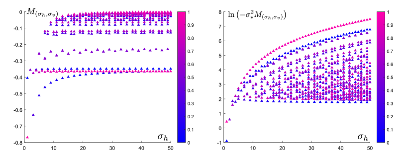
Figure 4: These plots represent the outcome of our numerical computations for the values $M_{(\sigma_{h},\sigma_{v})}$, where we used $g(u;a)=6u(u-1)(u-a)$ with $a=0.45$. For each fixed $\sigma_{h}$ (horizontal) we computed these values for each integer $1\leq\sigma_{v}\leq\sigma_{h}$ that has $\mathrm{gcd}(\sigma_{h},\sigma_{v})=1$, using the color code to represent the fraction ${\sigma_{v}}/{\sigma_{h}}$. On the left we see the formation of horizontal bands of the same color, suggesting the possibility to take limits along convergent subsequences $({\sigma_{v}^{(n)}}/{\sigma_{h}^{(n)}})_{n>0}$; see also Figure 5. The $\sigma_{*}^{2}$-scaling on the right shows that our condition requiring $M_{(\sigma_{h},\sigma_{v})}$ to be negative can be confirmed in a robust fashion.

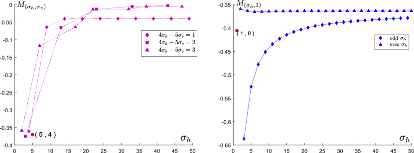
Figure 5: These plots track the values of $M_{(\sigma_{h},\sigma_{v})}$ along several subsequences of fractions $\sigma_{v}/\sigma_{h}$ that converge to $4/5$ (left) or zero (right). In all cases the limits are strictly above the values $M_{(5,4)}$ (left) and $M_{(1,0)}$ (right) corresponding to the limiting angles, supporting the inequality (2.51).

$k$	1	2	3	4	5	6	7	8	9	10
$a_{k}$	0	0.896	0.195	0.068	0.966	0	-0.143	0	0	0.05
$a_{-k}$	0	0.912	0.0925	0.179	1.005	0	-0.199	0	0	0.03

Table 1: Numerically computed values for the coefficients $(a_{k})$ defined in (2.23) for the propagation direction $(\sigma_{h},\sigma_{v})=(2,5)$, with the nonlinearity $g(u;a)=6u(u-1)(u-0.45)$. We computed these coefficients for a large range of angles and used them to calculate the values $M_{(\sigma_{h},\sigma_{v})}$ depicted in Figures 4-5.

Our goal here is to numerically investigate the condition (HS$)_{2}$. In order to compensate for the fact that $f$ is locally quadratic around $0$, we calculated the values

$$M_{(\sigma_{h},\sigma_{v})}:=\sup_{0<|\omega|\leq\pi}\frac{f_{(\sigma_{h},\sigma_{v})}(\omega)}{\omega^{2}}$$

for a large range of parameters $(\sigma_{h},\sigma_{v})\in\mathbb{Z}^{2}$.

As a first step, we numerically solved the coupled set of equations

$$-c_{*}\Phi_{*}^{\prime}(\xi) =\Phi_{*}(\xi+\sigma_{h})+\Phi_{*}(\xi-\sigma_{h})+\Phi_{*}(\xi+\sigma_{v})+\Phi_{*}(\xi-\sigma_{v})-4\Phi_{*}(\xi)+g\big{(}\Phi_{*}(\xi)\big{)},$$ (2.46)

$$c_{*}\psi_{*}^{\prime}(\xi) =\psi_{*}(\xi+\sigma_{h})+\psi_{*}(\xi-\sigma_{h})+\psi_{*}(\xi+\sigma_{v})+\psi_{*}(\xi-\sigma_{v})-4\psi_{*}(\xi)+g^{\prime}\big{(}\Phi_{*}(\xi)\big{)}\psi_{*}(\xi)$$ (2.47)

on a domain $[-L,L]$ for some large $L\gg 1$, using the boundary conditions

$$\Phi_{*}(-L)=0,\qquad\Phi_{*}(L)=1,\qquad\psi_{*}(\pm L)=0.$$

Due to the fact that the solutions are shift-invariant, we also fixed $\Phi(0)=\frac{1}{2}$ and $\psi(0)=1$. In order to overcome the issue that $L$ needs to be very large when $\sigma_{h}$ or $\sigma_{v}$ is large, we used the representation

$$\sigma_{*}=\sqrt{\sigma_{h}^{2}+\sigma_{v}^{2}},\qquad(\sigma_{h},\sigma_{v})=\sigma_{*}(\cos\zeta_{*},\sin\zeta_{*})$$

to introduce the rescaled functions

$$\tilde{\Phi}(\xi):=\Phi_{*}({\xi}/{\sigma_{*}}),\qquad\tilde{\psi}(\xi):=\psi_{*}({\xi}/{\sigma_{*}}).$$

These must satisfy the equivalent system of equations

$$-\frac{c_{*}}{\sigma_{*}}\tilde{\Phi}^{\prime}(\xi) =\tilde{\Phi}(\xi+\cos\zeta_{*})+\tilde{\Phi}(\xi-\cos\zeta_{*})+\tilde{\Phi}(\xi+\sin\zeta_{*})+\tilde{\Phi}(\xi-\sin\zeta_{*})+g\big{(}\tilde{\Phi}(\xi)\big{)}$$ (2.48)

$$\frac{c_{*}}{\sigma_{*}}\tilde{\psi}^{\prime}(\xi) =\tilde{\psi}(\xi+\cos\zeta_{*})+\tilde{\psi}(\xi-\cos\zeta_{*})+\tilde{\psi}(\xi+\sin\zeta_{*})+\tilde{\psi}(\xi-\sin\zeta_{*})+g^{\prime}\big{(}\tilde{\Phi}(\xi)\big{)}\tilde{\psi}(\zeta),$$ (2.49)

which allowed us to keep $L$ fixed and use a continuation approach to vary the angle $\zeta_{*}$.

We discretized the domain by dividing the segment $[-L,L]$ into $N_{L}$ parts of size $\Delta\xi$ for some integer $N_{L}\gg 1$ and step size $\Delta\xi\ll 1$, discretizing the first derivatives in (2.48)-(2.49) by the fourth-order central difference scheme. We proceeded by using a nonlinear system solver to obtain the speed $c$ and the values $\big{(}\tilde{\Phi}(\xi_{n}),\tilde{\psi}(\xi_{n})\big{)}$ in the nodes $\xi_{n}=-L+n\Delta\xi$, for $n=0,\dots N_{L}$. We subsequently used these values to solve the systems (2.18) and compute the coefficients needed to construct the function $f_{(\sigma_{h},\sigma_{v})}$ defined in (2.24). As an example, in Table 1 we present the values of $(a_{k})$ for the angle of propagation $(2,5)$, noting that both positive and negative values occur.

Our full results are visualized in Figures 4 and 5. In all cases the value $M_{(\sigma_{h},\sigma_{v})}$ was negative, hence validating (HS$)_{2}$. In addition, we observed that if we pick a sequence of angles $(\sigma_{h}^{n},\sigma_{v}^{n})$ for which we have the convergence

$$\lim_{n\to\infty}\sigma_{v}^{n}/\sigma_{h}^{n}=\sigma_{v}^{*}/\sigma_{h}^{*}$$ (2.50)

for some pair $(\sigma_{h}^{*},\sigma_{v}^{*})\in\mathbb{Z}^{2}$ not contained in this sequence, then

$$\liminf_{n\to\infty}M_{(\sigma_{h}^{n},\sigma_{v}^{n})}>M_{(\sigma_{h}^{*},\sigma_{v}^{*})}.$$ (2.51)

This behaviour closely resembles the crystallographic pinning phenomenon discussed in [18, 32], where the role of $M$ is played by the direction-dependent boundary of the parameters $a$ where the wave is pinned ($c_{*}=0$).

3 Omega limit points

Both the construction of the phase $\gamma$ as well as the proof of Proposition 2.7 rely heavily on the properties of so-called $\omega$-limit points. Intuitively, these track the long-time behaviour of $u$ after correcting for the velocity of the planar wave. To be more precise, let us consider a sequence in ${\mathbb{Z}^{2}_{\times}}\times{\mathbb{R}}$ that is taken from the subset

$$\mathcal{S}=\left\{(n_{k},l_{k},t_{k})_{k\geq 0}:0<t_{1}<t_{2}<\dots\to\infty,\ |n_{k}-ct_{k}|\leq M\text{ for some }M>0\right\}.$$ (3.1)

For any solution $u\in C^{1}\left([0,\infty),\ell^{\infty}(\mathbb{Z}_{\times}^{2})\right)$, our goal is to analyze the limiting behaviour of the shifted solutions $u_{n+n_{k},l+l_{k}}(t+t_{k})$. In the special case that $u$ is the exact planar wave solution

$$u_{n,l}(t)=\Phi_{*}(n-c_{*}t),$$

the fact that the sequence $n_{k}-c_{*}t_{k}$ is bounded allows us to find a constant $\theta_{0}\in{\mathbb{R}}$ for which the convergence

$$u_{n+n_{k},l+l_{k}}(t+t_{k})=\Phi_{*}(n+n_{k}-c_{*}t-c_{*}t_{k})\to\Phi_{*}(n-c_{*}t+\theta_{0})$$ (3.2)

holds on some subsequence. The limiting function is hence equal to our planar wave, albeit with a perturbed phase $\theta_{0}$.

Our main result here states that the convergence result (3.2) continues to hold for a much larger set of solutions of the discrete Allen-Cahn equation (2.6). This generalizes our earlier results in [23] where we only considered horizontal directions. Although some minor technical obstacles need to be resolved, the main principles are comparable. In fact, we actually sharpened the setup slightly by avoiding the superfluous usage of the floor and ceiling functions in [23, Prop. 3.1]. This allows for a more efficient and readable analysis here and in the sequel.

Proposition 3.1.

Suppose that (H$g$), (H$\Phi$) and (H$0$) hold and let $u$ be a solution of (2.6) with the initial condition (2.7). Then for any sequence $(n_{k},l_{k},t_{k})_{k\geq 0}\in\mathcal{S}$ there exists a subsequence $(n_{i_{k}},l_{i_{k}},t_{i_{k}})_{k\geq 0}$ and a shift $\theta_{0}\in{\mathbb{R}}$ such that

$$u_{n+n_{i_{k}},l+l_{i_{k}}}(t+t_{i_{k}})\to\Phi_{*}(n-c_{*}t+\theta_{0})\quad\text{in}\quad C_{\mathrm{loc}}(\mathbb{Z}_{\times}^{2}\times{\mathbb{R}}).$$ (3.3)

The proof follows directly by combining the two main ingredients that we state below. First, in Proposition 3.2, we use Arzela-Ascoli to construct a solution $\omega\in C^{1}\left({\mathbb{R}};\ell^{\infty}(\mathbb{Z}_{\times}^{2})\right)$ to the discrete Allen-Cahn equation (2.6) on $\mathbb{Z}_{\times}^{2}\times{\mathbb{R}}$ as a limit of the sequence $u_{n+n_{k},l+l_{k}}(t+t_{k})$. Furthermore, we show that this solution $\omega$ lies between two travelling waves. Proposition 3.3 subsequently states that this latter property is sufficient to guarantee that $\omega$ is a travelling wave itself. This transfers the comparable result in [5] from the continuous to the discrete setting.

Proposition 3.2.

Consider the setting of Proposition 3.1 and pick a sequence $(n_{k},l_{k},t_{k})_{k\geq 0}\in\mathcal{S}$. Then there exists a subsequence $(n_{i_{k}},l_{i_{k}},t_{i_{k}})_{k\geq 0}$ and a function $\omega\in C^{1}({\mathbb{R}};\ell^{\infty}(\mathbb{Z}_{\times}^{2}))$ that satisfy the following claims.

1. We have the convergence

   $$u_{n+n_{i_{k}},l+l_{i_{k}}}(t+t_{i_{k}})\to\omega_{n,l}(t)\quad\text{in}\ C_{\text{loc}}(\mathbb{Z}_{\times}^{2}\times{\mathbb{R}}).$$ (3.4)

2. The function $\omega$ satisfies the discrete Allen-Cahn equation (2.6) on ${\mathbb{Z}^{2}_{\times}}\times{\mathbb{R}}$.

3. There exists a constant $\theta\in{\mathbb{R}}$ such that

   $$\Phi_{*}(n-c_{*}t-\theta)\leq\omega_{n,l}(t)\leq\Phi_{*}(n-c_{*}t+\theta),\quad\text{for all}\ (n,l)\in\mathbb{Z}_{\times}^{2}.$$ (3.5)

Proposition 3.3.

Assume that (H$g$) and (H$\Phi$) are satisfied and consider a function $\omega\in C^{1}\left({\mathbb{R}};\ell^{\infty}(\mathbb{Z}_{\times}^{2})\right)$ that satisfies the Allen-Cahn LDE (2.6) for all $t\in{\mathbb{R}}$. Assume furthermore that there exists a constant $\theta$ for which the bounds

$$\Phi_{*}(n-c_{*}t-\theta)\leq\omega_{n,l}(t)\leq\Phi_{*}(n-c_{*}t+\theta)$$ (3.6)

hold for all $(n,l)\in\mathbb{Z}_{\times}^{2}$ and $t\in{\mathbb{R}}$. Then there exists a constant $\theta_{0}\in[-\theta,\theta]$ so that

$$\omega_{n,l}(t)=\Phi_{*}(n-c_{*}t+\theta_{0}),\quad\hbox{for all }(n,l)\in\mathbb{Z}_{\times}^{2},\,t\in{\mathbb{R}}.$$ (3.7)

Proof of Proposition 3.1.

The claim follows directly from Propositions 3.2 and 3.3. ∎

3.1 Construction of $\omega$

Our first result provides preliminary upper and lower bounds for the solution $u$. It is based upon a standard comparison principle argument that can be traced back to Fife and Mcleod [14].

Lemma 3.4.

Assume that (Hg), $(H\Phi)$ and (H0) are satisfied. Then there exists a time $T>0$ together with constants

$$q_{1}\in(0,a),\qquad q_{2}\in(0,1-a),\qquad\theta_{1}\in{\mathbb{R}},\qquad\theta_{2}\in{\mathbb{R}},\qquad\mu>0,\qquad C>0$$ (3.8)

so that the solution $u$ to (2.6) with the initial condition (2.7) satisfies the estimates

$$u_{n,l}(t)\leq\Phi_{*}\left(n+\theta_{1}-c_{*}(t-T)+Cq_{1}\big{(}1-e^{-\mu(t-T)}\big{)}\right)+q_{1}e^{-\mu(t-T)},\quad\forall t\geq T,$$ (3.9)

$$u_{n,l}(t)\geq\Phi_{*}\left(n-\theta_{2}-c_{*}(t-T)-Cq_{2}\big{(}1-e^{-\mu(t-T)}\big{)}\right)-q_{2}e^{-\mu(t-T)},\quad\forall t\geq T.$$ (3.10)

Proof.

The result can be shown by following the procedure outlined in the proof of Lemma 3.5 in [23], using the inequality

$$\alpha|c_{*}|-2(\cosh{\sigma_{h}c_{*}}-1)-2(\cosh{\sigma_{v}c_{*}}-1)\geq\dfrac{2K}{a-d}$$

to replace (3.14) in [23] and modifying the definition (3.16) in [23] to read

$$w_{n,l}(t)=d+Me^{|c_{*}|(n+\alpha t)}.$$

∎

Proof of Proposition 3.2.

Fix an integer $T\in{\mathbb{N}}$ and denote by $M_{T}$ the number of points in $\mathbb{Z}_{\times}^{2}$ that are also contained in the square $[-T,T]^{2}$, i.e. $M_{T}=\#\left\{(n,l)\in\mathbb{Z}_{\times}^{2}\cap[-T,T]^{2}\right\}$. Consider the functions

$$u^{k}\in C\left([-T,T];{\mathbb{R}}^{M_{T}\times M_{T}}\right)$$

that are defined by

$$u^{k}_{n,l}(t)=u_{n+n_{k},l+l_{k}}(t+t_{k})$$

for all sufficiently large $k$. From Lemma 3.4 it follows that the solution $u$ and consequently the functions $u^{k}$ are globally bounded, which in view of (2.6) implies that the same holds for the derivative $\dot{u}$. The sequence $u^{k}$ hence satisfies the conditions of the Arzela-Ascoli theorem and is thus relatively compact in $C\left([-T,T];{\mathbb{R}}^{M_{T}\times M_{T}}\right)$. Applying (2.6) and using a standard diagonalisation argument, we obtain a subsequence $u^{i_{k}}$ and a function $\omega:{\mathbb{R}}\to\ell^{\infty}(\mathbb{Z}_{\times}^{2})$ for which the convergence

$$\sup_{(n,l,t)\in K}|u^{i_{k}}_{n,l}(t)-\omega_{n,l}(t)|+|\dot{u}^{i_{k}}_{n,l}(t)-\dot{\omega}_{n,l}(t)|\to 0$$ (3.11)

holds for every compact $K\subset\mathbb{Z}_{\times}^{2}\times{\mathbb{R}}$. This yields items (i) and (ii), while item (iii) follows from Lemma 3.4. ∎

3.2 Trapped entire solutions

The main aim of this subsection is to establish Proposition 3.3, which states that every entire solution of the discrete Allen-Cahn equation on ${\mathbb{Z}^{2}_{\times}}\times{\mathbb{R}}$ trapped between two travelling waves is a travelling wave itself. At the heart of the proof lies a version of the maximum principle for LDEs which we provide below in Lemmas 3.5 and 3.6. As a preparation, we define the quantities

$$\sigma_{\infty}:=\max\{|\sigma_{h}|,|\sigma_{v}|\},\qquad m_{*}:=\sigma_{\infty}-1.$$ (3.12)

Lemma 3.5.

Pick $\kappa\in{\mathbb{R}}$ and let $E_{\kappa}\subset\mathbb{Z}^{2}_{\times}\times{\mathbb{R}}$ be defined as

$$E_{\kappa}=\left\{(n,l,t)\in\mathbb{Z}^{2}_{\times}\times{\mathbb{R}}:n-c_{*}t\geq\kappa\right\}.$$ (3.13)

Pick $B\in{\mathbb{R}}$ and $\epsilon>0$ and assume that the function $z\in C^{1}\big{(}{\mathbb{R}},\ell^{\infty}(\mathbb{Z}^{2}_{\times})\big{)}$ satisfies the conditions

1. $z_{n,l}(t)\geq 0$ for all $(n,l,t)\in E_{\kappa}$;

2. $z_{n,l}(t)\geq\epsilon$ for all $(n,l,t)\in E_{\kappa}$ with $n-c_{*}t\in[\kappa,\kappa+m_{*}]$;

3. $\dot{z}_{n,l}(t)-(\Delta^{\times}z)_{n,l}(t)+Bz_{n,l}(t)\geq 0$ for all $(n,l,t)\in E_{\kappa}$.

Then, in fact $z_{n,l}(t)>0$ for all $(n,l,t)\in E_{\kappa}$.

Proof.

Assume to the contrary that there exists $(n_{0},l_{0},t_{0})\in E_{\kappa}$ for which $z_{n_{0},l_{0}}(t_{0})=0$. Since the function $z$ attains its minimum at this interior point, we know that $\dot{z}_{n_{0},l_{0}}(t_{0})=0$. In addition, assumption (ii) ensures that $(\Delta^{\times}z)_{n_{0},l_{0}}(t_{0})\geq 0$. On the other hand, assumption (iii) gives

$$0\leq\dot{z}_{n_{0},l_{0}}(t_{0})-(\Delta^{\times}z)_{n_{0},l_{0}}(t_{0})+Bz_{n_{0},l_{0}}(t_{0})=-(\Delta^{\times}z)_{n_{0},l_{0}}(t_{0})\leq 0.$$

Therefore, the equality $(\Delta^{\times}z)_{n_{0},l_{0}}(t_{0})=0$ must hold. In particular, we have

$$z_{n_{0}-\sigma_{h},l-\sigma_{v}}(t_{0})=z_{n_{0}+\sigma_{h},l+\sigma_{v}}(t_{0})=z_{n_{0}-\sigma_{v},l+\sigma_{h}}(t_{0})=z_{n_{0}+\sigma_{v},l-\sigma_{h}}(t_{0})=0.$$

We note that the inclusion

$$n_{0}-\sigma_{\infty}\in[\kappa,\kappa+m_{*}]$$

would immediately contradict property (ii). On the other hand, if

$$n_{0}-\sigma_{\infty}~{}\geq\kappa+m_{*}+1$$

we can repeat this procedure with $n_{0}-\sigma_{\infty}$ until the desired contradiction is reached. ∎

Lemma 3.6.

Pick $\kappa\in{\mathbb{R}}$ and let $F_{\kappa}\subset\mathbb{Z}^{2}_{\times}\times{\mathbb{R}}$ be defined as

$$F_{\kappa}=\left\{(n,l,t)\in\mathbb{Z}^{2}_{\times}\times{\mathbb{R}}:n-c_{*}t\leq\kappa\right\}.$$ (3.14)

Pick $B\in{\mathbb{R}}$ and $\epsilon>0$ and assume that the function $z\in C^{1}({\mathbb{R}},\ell^{\infty}\big{(}\mathbb{Z}^{2}_{\times})\big{)}$ satisfies the conditions

1. $z_{n,l}(t)\geq 0$ for $(n,l,t)\in F_{\kappa}$;

2. $z_{n,l}(t)\geq\epsilon$ for all $(n,l,t)\in F_{\kappa}$ with $n-c_{*}t\in[\kappa-m_{*},\kappa]$;

3. $\dot{z}_{n,l}(t)-(\Delta^{\times}z)_{n,l}(t)+Bz_{n,l}(t)\geq 0$ for all $(n,l,t)\in F_{\kappa}$.

Then, in fact $z_{n,l}(t)>0$ on $F_{\kappa}$.

Proof.

The proof is almost identical to that of Lemma 3.5. ∎

Lemma 3.7.

Consider the setting of Proposition 3.3 and pick a sufficiently small $\delta>0$. Choose a pair $(N,L)\in\mathbb{Z}_{\times}^{2}$ together with a constant $\rho\in{\mathbb{R}}$. Suppose for some $\kappa\in\mathbb{Z}$ that the function

$$v^{\rho}_{n,l}(t)=\omega_{n+N,l+L}\left(t+{N}/{c_{*}}+{\rho}/{c_{*}}\right)$$ (3.15)

satisfies the inequality

$$v^{\rho}_{n,l}(t)\leq\omega_{n,l}(t)$$ (3.16)

whenever $n-c_{*}t\in[\kappa,\kappa+m_{*}]$. Then the following claims holds true.

1. If $\omega_{n,l}(t)\geq 1-\delta$ whenever $n-c_{*}t\geq\kappa$, then in fact (3.16) holds for all $n-c_{*}t\geq\kappa$.

2. If $v^{\rho}_{n,l}(t)\leq\delta$ whenever $n-c_{*}t\leq\kappa+m_{*}$, then in fact (3.16) holds for all $n-c_{*}t\leq\kappa+m_{*}$.

Proof.

We follow the outline of the proof from [23, §4], which can be seen as a spatially discrete version of [5, §3] where continuous travelling waves were considered. We only establish (i), since (ii) can be obtained in a similar fashion using the set $F_{\kappa}$ from Lemma 3.6 instead of the set $E_{\kappa}$ from Lemma 3.5.

Due to the global bounds on the functions $\omega$ and $v^{\rho}$, the quantity

$$\epsilon^{*}=\inf\left\{\epsilon>0:v^{\rho}\leq\omega+\epsilon\ \text{in}\ E_{\kappa}\right\}$$ (3.17)

is finite and by continuity we have

$$v^{\rho}\leq\omega+\epsilon^{*}\quad\text{in}\ E_{\kappa}.$$ (3.18)

To prove the claim we must show that $\epsilon^{*}=0$.

Assuming to the contrary that $\epsilon^{*}>0$, we find sequences $(n_{k},l_{k},t_{k})\in E_{\kappa}$ and $\epsilon_{k}\nearrow\epsilon^{*}$ such that

$$\omega_{n_{k},l_{k}}(t_{k})+\epsilon_{k}<v^{\rho}_{n_{k},l_{k}}(t_{k})\leq\omega_{n_{k},l_{k}}(t_{k})+\epsilon^{*}.$$ (3.19)

The right inequality above together with the bounds (3.6) implies that the sequence $n_{k}-c_{*}t_{k}$ is bounded. Applying a similar construction to that in the proof of Corollary 3.2, we obtain a function $\omega^{\infty}\in C^{1}\left({\mathbb{R}};\ell^{\infty}({\mathbb{Z}^{2}_{\times}})\right)$ for which we have the limits

$$\lim_{k\to\infty}\omega_{n+n_{k},l+l_{k}}(t+t_{k})=\omega^{\infty}_{n,l}(t),$$ (3.20)

$$\lim_{k\to\infty}v^{\rho}_{n+n_{k},l+l_{k}}(t+t_{k})=\omega^{\infty}_{n+N,l+L}\left(t+N/c_{*}+\rho/c_{*}\right).$$

We define the function $z\in C^{1}\left({\mathbb{R}},\ell^{\infty}({\mathbb{Z}^{2}_{\times}})\right)$ by

$$z_{n,l}(t)=\omega^{\infty}_{n,l}(t)-\omega^{\infty}_{n+N,l+L}(t)+\epsilon^{*}$$ (3.21)

and claim that $z$ satisfies conditions (i)-(iii) of Lemma 3.5 on the set

$$E_{0}=\left\{(n,l,t)\in{\mathbb{Z}^{2}_{\times}}\times{\mathbb{R}}:n-c_{*}t\geq 0\right\}.$$

To see this, we first note that $n+n_{k}-c_{*}t-c_{*}t_{k}\geq\kappa$ holds by construction on the set $E_{0}$. Since the inequality (3.18) survives the limit (3.20), we have $z_{n,l}(t)\geq 0$ on $E_{0}$, verifying (i). Turning to (ii), we note that the inequality (3.16) implies that

$$z_{n,l}(t)\geq\epsilon^{*}>0,\ \qquad\text{for}\ n-c_{*}t\in[0,m_{*}].$$

To establish (iii), we pick $\delta>0$ in such a way that the function $g$ is non-increasing on the interval $[1-\delta,1]$. Recalling that $\omega^{\infty}\in[1-\delta,1]$ on $E_{0}$ and that $g$ is locally Lipschitz, we obtain the bound

$$\dot{z}_{n,l}(t)-(\Delta^{\times}z)_{n,l}(t) =g\big{(}\omega^{\infty}_{n,l}(t)\big{)}-g\big{(}\omega^{\infty}_{n+N,l+L}(t)\big{)}$$

$$\geq g(\omega^{\infty}_{n,l}(t)+\epsilon^{*})-g\big{(}\omega^{\infty}_{n+N,l+L}(t)\big{)}$$

$$\geq-Bz_{n,l}(t)$$

for any $(n,l,t)\in E_{0}$. We may hence apply Lemma 3.5 and conclude that $z>0$ on $E_{0}$. However, the inequalities (3.19) imply that $z_{0,0}(0)=0$, which is a contradiction. Therefore $\epsilon^{*}=0$ must hold, as desired. ∎

Lemma 3.8.

Consider the setting of Propostion 3.3, fix an arbitrary pair $(N,L)\in\mathbb{Z}^{2}$ and recall the functions $v^{\rho}$ defined in (3.15). Then the quantity

$$\rho_{*}:=\inf\left\{\rho\in{\mathbb{R}}:v^{\tilde{\rho}}\leq\omega\text{ in }{\mathbb{Z}^{2}_{\times}}\times{\mathbb{R}}\text{ for all }\tilde{\rho}\geq\rho\right\}$$ (3.22)

satisfies $\rho_{*}\leq 0$.

Proof.

One can obtain this result by following the outline presented in the proof of [23, Lemma 4.4]. Instead of [23, Lemma 4.3], one now needs to employ Lemma 3.7. ∎

Proof of Proposition 3.3.

From Lemma 3.8, it follows that

$$\omega_{n,l}(t)\geq\omega_{n+N,l+L}(t+{N}/{c_{*}})\quad\text{on }{\mathbb{Z}^{2}_{\times}}\times{\mathbb{R}}.$$ (3.23)

Since the pair $(N,L)\in\mathbb{Z}_{\times}^{2}$ is arbitrary, we can conclude that the function $\omega$ depends only on the difference $n-c_{*}t$. In particular, there exists a function $\varphi$ such that $\omega_{n,l}(t)=\varphi(n-c_{*}t)$. The result now follows directly from the fact that solutions to the travelling wave problem (2.10)-(2.11) for $c_{*}\neq 0$ are unique up to translation; see [31]. ∎

4 Large time behaviour of $u$

In this section we establish Proposition 2.7 by studying the qualitative large time behaviour of the solution $u$ within the interfacial region

$$I_{t}=\left\{(n,l)\in{\mathbb{Z}^{2}_{\times}}:\Phi_{*}\left(-\sigma_{*}^{2}-1\right)\leq u_{n,l}(t)\leq\Phi_{*}\left(\sigma_{*}^{2}+1\right)\right\},$$ (4.1)

which represents the points at which a solution $u$ is close to $\Phi_{*}(0)=1/2$. The boundary values $\Phi_{*}(-\sigma_{*}^{2}-1)$ and $\Phi_{*}(\sigma_{*}^{2}+1)$ were carefully chosen to ensure that $I_{t}$ is nonempty for large $t$, which we show in Proposition 4.1. In addition, we show that for a fixed pair $(l,t)$ the map $n\mapsto u_{n,l}(t)$ is monotone within $I_{t}$, in the sense that the differences $u_{n+\sigma_{*}^{2},l}(t)-u_{n,l}(t)$ are bounded from below uniformly in time.

In addition to the monotonicity within $I_{t}$, the map $n\mapsto u_{n,l}(t)$ cannot exit throughout the lower boundary once it enters the interfacial region from below. Similarly, it cannot reenter the interval once it has left through the upper boundary. All together, these results provide sufficient control in the crucial region away from the stable equilibria zero and one to uniquely define the phase $\gamma$ by the procedure described in §2.2.

The results of this section are a generalization of the results presented in [23, §5], requiring us to take into account several technical differences that arise due to the additional complexities of working with ${\mathbb{Z}^{2}_{\times}}$ rather than $\mathbb{Z}^{2}$. Moreover, our construction of the phase $\gamma(t)$ here is more refined than the setup in  [23], which also causes several modifications to the proofs.

Proposition 4.1.

Consider the setting of Proposition 2.7. Then there exists $T>0$ such that the following claims hold true.

1. For each $t\geq T$ and $l\in\mathbb{Z}$ there exists $n_{*}=n_{*}(l,t)\in\mathbb{Z}$ for which

   $$\Phi_{*}(-\sigma_{*}^{2}-1)<u_{n_{*},l}(t)\leq\frac{1}{2}.$$ (4.2)

2. We have the inequality

   $$\inf_{t\geq T,\,(n,l)\in I_{t}}u_{n+\sigma_{*}^{2},l}(t)-u_{n,l}(t)>0.$$ (4.3)

3. Consider any $t\geq T$ and $(n,l)\in{\mathbb{Z}^{2}_{\times}}$ for which $u_{n,l}(t)\leq\Phi_{*}(-\sigma_{*}^{2}-1)$ holds. Then we also have $u_{n-\sigma_{*}^{2},l}(t)\leq\Phi_{*}(-\sigma_{*}^{2}-1)$.

4. Consider any $t\geq T$ and $(n,l)\in{\mathbb{Z}^{2}_{\times}}$ for which $u_{n,l}(t)\geq\Phi_{*}(\sigma_{*}^{2}+1)$ holds. Then we also have $u_{n+\sigma_{*}^{2},l}(t)\geq\Phi_{*}(\sigma_{*}^{2}+1)$.

Proof of Proposition 2.6.

The statement follows directly from item i of Proposition 4.1. ∎

In the following proposition we provide an asymptotic flatness result for the phase $\gamma$. This feature is a crucial property that allows us to construct the super- and sub-solutions that we use in the proof of Theorem 2.9 and consequently Theorem 2.10.

Proposition 4.2.

Consider the setting of the Proposition 4.1 and recall the phase $\gamma:[T,\infty)\to\ell^{\infty}(\mathbb{Z})$ defined in (2.34). Then we have the limit

$$\lim_{t\to\infty}\sup_{l\in\mathbb{Z}}|\gamma_{l+1}(t)-\gamma_{l}(t)|=0.$$

4.1 Phase construction

In this subsection we prove Proposition 4.1, mainly by relying on the convergence results from Proposition 3.1. As a preparation, we define the set

$$\mathcal{I}(T,R):=\left\{(n,l,t)\in{\mathbb{Z}^{2}_{\times}}\times[T,\infty):|n-c_{*}t|\leq R\right\}$$ (4.4)

for any pair of positive constants $T$ and $R$ and we also remind the reader of the set of sequences $\mathcal{S}$ defined in (3.1).

Lemma 4.3.

Consider the setting of Proposition 4.1 and pick a constant $R>0$. Then there exists a constant $T>0$ such that

$$\inf_{(n,l,t)\in\mathcal{I}(T,R)}u_{n+\sigma_{*}^{2},l}(t)-u_{n,l}(t)>0.$$

Proof.

Assume to the contrary that there exists a constant $R>0$ such that

$$\inf_{(n,l,t)\in\mathcal{I}(T,R)}u_{n+\sigma_{*}^{2},l}(t)-u_{n,l}(t)\leq 0$$ (4.5)

holds for every $T>0$. That implies that we can find a sequence $(n_{k},l_{k},t_{k})_{k\geq 0}\in\mathcal{S}$ such that

$$u_{n_{k}+\sigma_{*}^{2},l_{k}}(t_{k})-u_{n_{k},l_{k}}(t_{k})\leq\dfrac{1}{k}.$$ (4.6)

By virtue of Proposition 3.1, we can find $\theta_{0}\in{\mathbb{R}}$ and pass to a subsequence for which we have the convergence

$$u_{n+n_{k},l+l_{k}}(t+t_{k})\to\Phi_{*}(n-c_{*}t+\theta_{0})\text{ in }C_{\text{loc}}({\mathbb{Z}^{2}_{\times}}\times{\mathbb{R}}).$$

Therefore, letting $k\to\infty$ in (4.6) leads to

$$\Phi_{*}(\sigma_{*}^{2}+\theta_{0})-\Phi_{*}(\theta_{0})\leq 0,$$ (4.7)

which contradicts the monotonicity of the function $\Phi_{*}$. ∎

Proof of Proposition 4.1.

We first establish (iv). Arguing by contradiction, assume that there exists a sequence $(n_{k},l_{k},t_{k})_{k\geq 0}$, $0<t_{1}<t_{2}<...\to\infty$ such that

$$u_{n_{k},l_{k}}(t_{k})\geq\Phi_{*}(\sigma_{*}^{2}+1)\quad\text{and}\quad u_{n_{k}+\sigma_{*}^{2},l_{k}}(t_{k})<\Phi_{*}(\sigma_{*}^{2}+1).$$ (4.8)

The bounds in Lemma 3.4 imply that the sequence $n_{k}-c_{*}t_{k}$ is bounded by some constant $R$. We can now apply Lemma 4.3 to conclude $u_{n_{k}+\sigma_{*}^{2},l_{k}}(t_{k})-u_{n_{k},l_{k}}(t_{k})>0$, which contradicts (4.8) due to the strict monotonicity of the function $\Phi_{*}$. Items (i) and (iii) follow in a similar way.

To prove item (ii), we choose a $T$ that satisfies (i), (iii) and (iv) and pick $t\geq T$ together with $(n,l)\in I_{t}$. Upon further increasing $T$, Lemma 3.4 implies that $n-c_{*}t$ is bounded by some constant $R>0$ that only depends on $T$. Therefore, we have shown that

$$\left\{(n,l,t):t\geq T,(n,l)\in I_{t}\right\}\subseteq\mathcal{I}(T,R).$$

The desired bound now follows directly from Lemma 4.3. ∎

Lemma 4.4.

Consider the setting of Proposition 4.1 and recall the phase $\gamma:[T,\infty)\to\ell^{\infty}(\mathbb{Z})$ defined in (2.34). Then there exists $T_{*}\geq T$ such that the difference $n_{*}(l,t)-c_{*}t$ is uniformly bounded for $t\geq T_{*}$ and $l\in\mathbb{Z}$ . In particular, we can find a constant $M>0$ so that

$$\left|\left|{\gamma(t)-c_{*}t}\right|\right|_{\ell^{\infty}}\leq M,\qquad\qquad t\geq T_{*}.$$

Proof.

The proof is analogous to that of Lemma 5.4 in [23]. ∎

Proof of Proposition 2.7.

Arguing by contradiction once more, let us assume that there exists $\delta>0$ together with sequences $(n_{k},l_{k})\in{\mathbb{Z}^{2}_{\times}}$ and $T\leq t_{1}<t_{2}<\dots\to\infty$ for which

$$|\Delta_{k}|:=|u_{n_{k},l_{k}}(t_{k})-\Phi_{*}\big{(}n_{k}-\gamma_{l_{k}}(t_{k})\big{)}|\geq\delta.$$ (4.9)

Analogously as in the proof of [23, Thm. 2.2], one can show that $n_{k}-c_{*}t_{k}$ is a bounded sequence. In addition, from Lemma 4.4 we also know that $n_{*}(l_{k},t_{k})-c_{*}t_{k}$ is bounded. Therefore, the sequence $n_{*}(l_{k},t_{k})-n_{k}$ is also bounded, allowing us to identify it with a constant $m\in\mathbb{Z}$. Applying Proposition 3.1 we find $\theta_{0}\in{\mathbb{R}}$ such that the limit

$$u_{n+n_{k},l+l_{k}}(t+t_{k})\to\Phi_{*}(n-c_{*}t+\theta_{0})$$ (4.10)

holds for all $(n,l,t)\in{\mathbb{Z}^{2}_{\times}}\times{\mathbb{R}}$, after passing to a further subsequence. Recalling the definition (2.34), this leads to

$$\Phi_{*}\big{(}n_{k}-\gamma_{l_{k}}(t_{k})\big{)} =\Phi_{*}\big{(}n_{k}-n_{*}(l_{k},t_{k})-\vartheta_{*}(l_{k},t_{k})\big{)}$$

$$=\Phi_{*}\big{(}-m-\vartheta_{*}(l_{k},t_{k})\big{)}.$$

Due to (4.10) and definition (2.31) of $\vartheta_{*}(l,t)$ we obtain the convergence

$$\vartheta_{*}(l_{k},t_{k})\to-\dfrac{\sigma_{*}^{2}\Phi_{*}^{-1}\big{(}\Phi_{*}(m+\theta_{0})\big{)}}{\Phi_{*}^{-1}\big{(}\Phi_{*}(m+\sigma_{*}^{2}+\theta_{0})\big{)}-\Phi_{*}^{-1}\big{(}\Phi_{*}(m+\theta_{0})\big{)}}=-m-\theta_{0}$$ (4.11)

as $k\to\infty$, which in turn implies that

$$\Phi_{*}\big{(}n_{k}-\gamma_{l_{k}}(t_{k})\big{)}\to\Phi_{*}(\theta_{0}).$$

We hence find that

$$\Delta_{k}\to\Phi_{*}(\theta_{0})-\Phi_{*}(\theta_{0})=0$$

as $k\to\infty$, which clearly contradicts (4.9). ∎

4.2 Phase asymptotics

In this subsection we establish the asymptotic flatness result for the phase $\gamma(t)$ that was stated in Proposition 4.2. A key ingredient is that the first differences of the function $l\mapsto n_{*}(l,t)$ can be uniformly bounded for large $t$.

Lemma 4.5.

Consider the setting of Proposition 4.1. Then there exists a constant $\tilde{T}>T$ so that for every $t\geq\tilde{T}$ and $l\in\mathbb{Z}$ we have

$$|n_{*}(l+1,t)-n_{*}(l,t)|\leq\sigma_{*}^{2}.$$

Proof.

Assume to the contrary that there exist sequences $(n_{k},\tilde{n}_{k},l_{k})_{k\geq 0}\subset\mathbb{Z}^{3}$, $(t_{k})_{k\geq 0}\subset(0,\infty)$ with $T<t_{1}<t_{2}<...\to\infty$ for which

$$|n_{k}-\tilde{n}_{k}|>\sigma_{*}^{2}$$ (4.12)

and

$$\begin{cases}u_{n_{k},l_{k}}(t_{k})\leq 1/2,\\ u_{n_{k}+\sigma_{*}^{2},l_{k}}(t_{k})>1/2,\end{cases}\qquad\qquad\qquad\qquad\begin{cases}u_{\tilde{n}_{k},l_{k}+1}(t_{k})\leq 1/2,\\ u_{\tilde{n}_{k}+\sigma_{*}^{2},l_{k}+1}(t_{k})>1/2.\end{cases}$$ (4.13)

Since both sequences $n_{*}(l_{k}+1,t_{k})-c_{*}t_{k}$ and $n_{*}(l_{k},t_{k})-c_{*}t_{k}$ are bounded, we can assume that their difference is constant and equal to $m\in\mathbb{Z}$, i.e.

$$m=\tilde{n}_{k}-n_{k}.$$

With this notation we can apply Proposition 3.1 to find a constant $\theta_{0}\in{\mathbb{R}}$ for which

$$\begin{cases}u_{n_{k},l_{k}}(t_{k})\to\Phi_{*}(\theta_{0}),\\ u_{n_{k}+\sigma_{*}^{2},l_{k}}(t_{k})\to\Phi_{*}(\theta_{0}+\sigma_{*}^{2}),\end{cases}\qquad\begin{cases}u_{m+{n}_{k},l_{k}+1}(t_{k})\to\Phi_{*}(m+\theta_{0}),\\ u_{m+\sigma_{*}^{2}+{n}_{k},l_{k}+1}(t_{k})\to\Phi_{*}(m+\theta_{0}+\sigma_{*}^{2}).\end{cases}$$

Combining these limits with the inequalities (4.13) we find that $\theta_{0}$ necessarily satisfies

$$-\sigma_{*}^{2}\leq\theta_{0}\leq 0,\qquad-\sigma_{*}^{2}\leq m+\theta_{0}\leq 0.$$

This in turn implies that $|m|\leq\sigma_{*}^{2}$, contradicting the strict inequality in (4.12).

∎

Proof of Proposition 4.2.

Assume to the contrary that there exists $\delta>0$ together with subsequences $(l_{k})_{k\geq 0}\subset\mathbb{Z}$ and $T\leq t_{1}<t_{2}<\dots\to\infty$ for which

$$\delta\leq|\gamma_{l_{k}+1}(t_{k})-\gamma_{l_{k}}(t_{k})|.$$ (4.14)

Lemma 4.5 assures us that it is possible to pass to a subsequence that has

$$n_{*}(l_{k}+1,t_{k})=n_{*}(l_{k},t_{k})+m,$$

for some integer $m\in[0,\sigma_{*}^{2}]$. Recalling the definition (2.31) for $\vartheta_{*}(l,t)$, we find

$$\gamma_{l_{k}+1}(t)-\gamma_{l_{k}}(t) =m+\vartheta_{*}(l_{k}+1,t_{k})-\vartheta_{*}(l_{k},t_{k}).$$ (4.15)

We now employ Proposition 3.1 to find $\theta_{0}\in{\mathbb{R}}$ such that for all $(n,l,t)\in{\mathbb{Z}^{2}_{\times}}\times{\mathbb{R}}$ we have

$$u_{n+n_{k},l+l_{k}}(t+t_{k})\to\Phi_{*}(n-c_{*}t+\theta_{0}),\quad\text{as}\quad k\to\infty,$$

which further implies that

$$\vartheta_{*}(l_{k},t_{k})\to-\theta_{0},\qquad\vartheta_{*}(l_{k}+1,t_{k})\to-m-\theta_{0}.$$

Taking the limit in (4.15) we obtain

$$\delta\leq|m-\theta_{0}-m+\theta_{0}|=0,$$

which is a clear contradiction. ∎

5 Linearized phase evolution

In this section we consider the lattice differential equation

$$\dot{h}_{l}(t)=\sum_{k=-N}^{N}a_{k}\big{[}h_{l+\mu_{k}}(t)-h_{l}(t)\big{]},\quad t>0$$ (5.1)

with the initial condition

$$h(0)=h^{0}\in\ell^{\infty}(\mathbb{Z}).$$ (5.2)

In order to highlight the general applicability of our results, we step back here from the specific framework associated to (2.38). Instead, we impose the following general assumption on the coefficients $a=(a_{k})_{k=-N}^{N}\subset{\mathbb{R}}$ and the shifts $\mu=(\mu_{k})_{k=-N}^{N}\subset\mathbb{Z}$.

• The function $f:[-\pi,\pi]\to{\mathbb{R}}$ defined by

  $$f(\omega):=\sum_{k=-N}^{N}a_{k}(\cos(\mu_{k}\omega)-1)$$ (5.3)

  is strictly negative on $[-\pi,\pi]\backslash\{0\}$. Futhermore, the constant $\Lambda\in{\mathbb{R}}$ defined by

  $$\Lambda:=\sum_{k=-N}^{N}a_{k}\mu_{k}^{2}=-f^{\prime\prime}(0)$$ (5.4)

  satisfies $\Lambda>0$.

Let us first observe that the assumption (h$\alpha$) implies that we can find $m>0$ and $\kappa>0$ such that

$$f(\omega) \leq-\dfrac{\Lambda}{2}\omega^{2}\ \text{for}\ \omega\in[-\kappa,\kappa],$$ (5.5)

$$f(\omega) <-m \text{for}\ \omega\in[-\pi,-\kappa]\cup[\kappa,\pi].$$ . (5.6)

For any $n\in{\mathbb{N}}_{0}$ we inductively define the $(n)$-th discrete derivative $\partial^{(n)}:\ell^{\infty}(\mathbb{Z})\to\ell^{\infty}(\mathbb{Z})$ by writing

$$[\partial^{(0)}\Gamma]_{j}:=\Gamma_{j},\qquad[\partial^{(1)}\Gamma]_{j}:=\Gamma_{j+1}-\Gamma_{j}$$

together with

$$[\partial^{(n)}\Gamma]_{j}=\left[\partial^{(1)}\left(\partial^{(n-1)}\Gamma)\right)\right]_{j}$$ (5.7)

for $n>1$. The first goal of this section is to establish decay estimates of the form

$$||\partial^{(n)}h(t)||_{\ell^{\infty}}\sim~{}O(t^{-\frac{n}{2}})$$ (5.8)

for the solution $h(t)$ of the system (5.1)-(5.2). These rates are consistent with the estimates for solutions of the continuous heat equation $h_{t}=h_{xx}$, which can be readily obtained by taking $x$-derivatives of the explicit representation

$$h(x,t)=\dfrac{1}{\sqrt{4\pi t}}\int_{{\mathbb{R}}}e^{-\frac{(x-y)^{2}}{4t}}h(y,0)dy.$$ (5.9)

Our goal is to find a solution formula for (5.1) equivalent to (5.9), in the sense that it takes the form of the convolution between the fundamental solution with the initial condition. By finding such a representation, we can transfer discrete derivatives onto the fundamental solution to establish (5.8).

Theorem 5.1 (see §5.1).

Assume that condition (h$\alpha$) holds and pick $n\in{\mathbb{N}}_{0}$. Then there exists a constant $C=C(n)$ so that for any $h^{0}\in\ell^{\infty}(\mathbb{Z})$, the $n$-th discrete derivative of the solution $h\in C^{1}\left([0,\infty);\ell^{\infty}(\mathbb{Z})\right)$ to the initial value problem (5.1)-(5.2) satisfies the bound

$$\left|\left|{\partial^{(n)}h(t)}\right|\right|_{\ell^{\infty}}\leq C\min\left\{\left|\left|{\partial^{(n)}h^{0}}\right|\right|_{\ell^{\infty}},\left|\left|{h^{0}}\right|\right|_{\ell^{\infty}}t^{-\frac{n}{2}}\right\}.$$

The second main result of this section concerns lower and upper bounds for the solution $h(t)$ that are sharper than the $\ell^{\infty}$-bounds in Theorem 5.1. In particular, we show that if the initial condition $h^{0}$ is bounded away from $0$, then the solution $h(t)$ is positive for large time $t\gg 1$. Moreover, under the additional assumption that the first differences of $h^{0}$ are flat enough we obtain the same conclusion for all time $t\geq 0$. The key issue is that some of the coefficients $(a_{k})$ are allowed to be negative, which causes the usual comparison principle to fail. Indeed, it can (and does) happen that a solution $h(t)$ admits negative values for a short time even if the initial condition is strictly positive.

Proposition 5.2 (see §5.1).

Consider the setting of Theorem 5.1 and pick $\varepsilon>0$. Then there exists a time $T=T(\varepsilon)>0$ and $C=C(T,\varepsilon)$ such that for all $t\geq T$ the following properties hold.

1. For any $h^{0}\in\ell^{\infty}(\mathbb{Z})$ that has $h_{k}^{0}\geq 0$ for all $k\in\mathbb{Z}$, we have the bounds

   $$h_{k}(t) \geq\inf_{j\in\mathbb{Z}}h^{0}_{j}-C\left|\left|{\partial h^{0}}\right|\right|_{\ell^{\infty}},\quad k\in\mathbb{Z},\qquad t\in[0,T],$$ (5.10)

   $$h_{k}(t) \geq\inf_{j\in\mathbb{Z}}h^{0}_{j}-\varepsilon\left|\left|{h^{0}}\right|\right|_{\ell^{\infty}}, k\in\mathbb{Z},\qquad t\geq T.$$ (5.11)

2. For any $h^{0}\in\ell^{\infty}(\mathbb{Z})$ that has $h_{k}^{0}\leq 0$ for all $k\in\mathbb{Z}$, we have the bounds

   $$h_{k}(t) \leq\sup_{j\in\mathbb{Z}}h^{0}_{j}+C\left|\left|{\partial h^{0}}\right|\right|_{\ell^{\infty}},\ \quad k\in\mathbb{Z},\qquad t\in[0,T],$$ (5.12)

   $$h_{k}(t) \leq\sup_{j\in\mathbb{Z}}h^{0}_{j}+\varepsilon\left|\left|{h_{0}}\right|\right|_{\ell^{\infty}}, k\in\mathbb{Z},\qquad t\geq T.$$ (5.13)

5.1 Strategy

In order to find an explicit formula for the solution $h$ of the initial problem (5.1)-(5.2), we note that a spatial Fourier transform leads to the decoupled sets of ODEs

$$\dfrac{d}{dt}\hat{h}(\omega,t)=\sum_{k=-N}^{N}a_{k}(e^{i\mu_{k}\omega}-1)\hat{h}(\omega,t)$$

for $\omega\in[-\pi,\pi]$. Introducing the function

$$p(\omega)=\sum_{k=-N}^{N}a_{k}\sin{(\mu_{k}\omega)},$$ (5.14)

we hence obtain the convolution formula

$$h_{l}(t)=\sum_{k\in\mathbb{Z}}h^{0}_{k}M_{l-k}(t),$$ (5.15)

where the fundamental solution $M(t)$ is defined by

$$M_{l}(t)=\dfrac{1}{2\pi}\int_{-\pi}^{\pi}e^{il\omega}e^{tf(\omega)+itp(\omega)}d\omega.$$ (5.16)

Notice that assumption (h$\alpha$) ensures that $\left|\left|{M(t)}\right|\right|_{\ell^{\infty}}\leq 1$ for every $t\geq 0$.

The proof of Theorem 5.1 relies on the following two lemmas, in which we focus on the decay estimates for the $\ell^{1}$-norm of the n-th differences $\partial^{(n)}M(t)$. We obtain the necessary estimates by dividing the sum into two parts, based on the size of the term $|l/t+a\cdot\mu|$. We note that the constant $-a\cdot\mu=-p^{\prime}(0)$ is often referred to as the group velocity. It tracks the speed of the ‘center’ of $M$ and - in context of §2 - is closely related to $[\partial_{\omega}\lambda_{\omega}]_{\omega=0}$ and $[\partial_{\varphi}c_{\varphi}]_{\varphi=0}$.

Lemma 5.3 (see §5.3).

Consider the setting of Theorem 5.1. Then there exist positive constants $K=K(n)$ and $C=C(n)$ such that

$$\sum_{|l/t+a\cdot\mu|\geq K}|[\partial^{n}M(t)]_{l}|\big{[}1+|l|\big{]}\leq Ce^{-t}.$$ (5.17)

Lemma 5.4 (see §5.4).

Consider the setting of Theorem 5.1 and pick $K>0$. Then there exists $C=C(K,n)>0$ such that

$$\sum_{|l/t+a\cdot\mu|\leq K}|[\partial^{n}M(t)]_{l}|\leq C\min\left\{1,t^{-\frac{n}{2}}\right\}.$$

Proof of Theorem 5.1.

In view of the convolution formula (5.15), we have

$$\left|\left|{\partial^{(n)}h(t)}\right|\right|_{\ell^{\infty}}\leq\left|\left|{h^{0}}\right|\right|_{\ell^{\infty}}\left|\left|{\partial^{(n)}M(t)}\right|\right|_{\ell^{1}}.$$

Employing Lemmas 5.3 and 5.4 in combination with the fast decay of the exponential we obtain a constant $C=C(n)$ for which

$$\left|\left|{\partial^{(n)}h(t)}\right|\right|_{\ell^{\infty}}\leq C\left|\left|{h^{0}}\right|\right|_{\ell^{\infty}}t^{-\frac{n}{2}}.$$

On the other hand, by transferring the n-th difference operators to the sequence $h^{0}$, we can write

$$\left|\left|{\partial^{(n)}h(t)}\right|\right|_{\ell^{\infty}}\leq\left|\left|{\partial^{(n)}h^{0}}\right|\right|_{\ell^{\infty}}\left|\left|{M(t)}\right|\right|_{\ell^{1}}.$$

Applying Lemmas 5.3 and 5.4 with $n=0$ now leads to the desired bound. ∎

To prove the lower bounds for solution $h(t)$ that are formulated in Proposition 5.2, we first note that

$$\sum_{l\in\mathbb{Z}}M_{l}(t)=1,\qquad t\geq 0.$$ (5.18)

Indeed, if $h^{0}\equiv 1$, then by uniqueness we must have $h(t)=1$ for all $t>0$. Our next task is to extract more detailed information on the spatial distribution of the ‘mass’ of $M$. In particular, we show that the bulk of this mass is contained in a region that is $O(\sqrt{t})$ wide. By combining our estimates with (5.18), the negative components of $M$ can be controlled asymptotically.

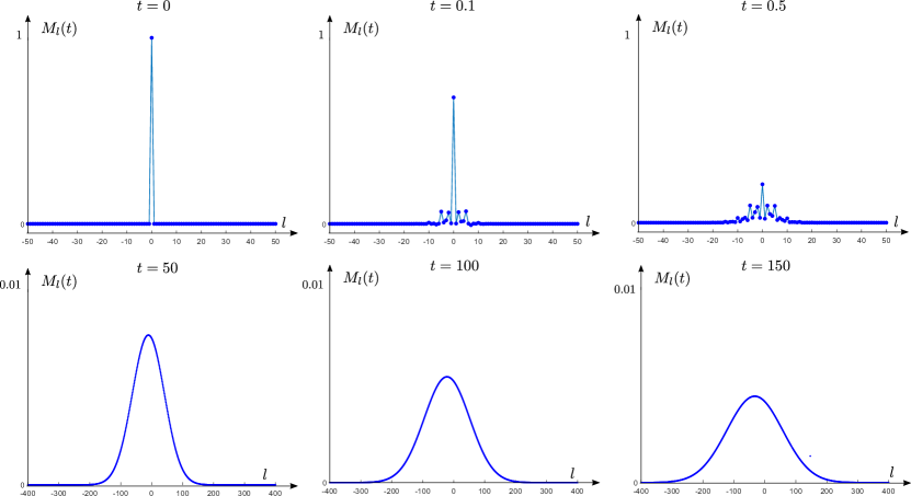
Figure 6: These six graphs represent the time evolution of the Green’s function $M_{l}(t)$, which we computed numerically by applying (5.16) to the coefficients $(a_{k})_{k=-10}^{10}$ appearing in Table 1. Observe the negative values for $M_{l}(t)$ that are clearly visible for $t=0.1$, together with the leftward movement of the ‘center of mass’, which travels at the speed $-a\cdot\mu=-0.22$.

Lemma 5.5 (see §5.4).

Consider the setting of Theorem 5.1 and pick positive constants $\kappa$ and $K_{*}$. Then there exist a time $T=T(\kappa,K_{*})$ such that for all $t\geq T$ we have

$$\sum_{|l/t+a\cdot\mu|\leq\frac{K_{*}}{\sqrt{t}}}|M_{l}(t)|\leq 1+\kappa.$$

Lemma 5.6 (see §5.4).

Consider the setting of Theorem 5.1 and pick $\kappa>0$. Then there exists a constant $K_{*}>0$ so that for all $K\geq K_{*}$ and $t\geq 1$ we have the bound

$$\sum_{\frac{K}{\sqrt{t}}\leq|l/t+a\cdot\mu|\leq K}|M_{l}(t)|\leq\kappa.$$

In our next result we show that the kernel $M(t)$ behaves similarly to the Gaussian kernel. In particular, for the continuous kernel we have

$$\dfrac{1}{\sqrt{t}}\int_{\mathbb{R}}e^{-x^{2}/t}\frac{|x|}{\sqrt{t}}\sim O(1).$$

To establish the equivalent estimate for the discrete kernel $M(t)$, we have to take into account that the kernel is not symmetric anymore, but that the center of mass ‘travels’ in time with speed $-(a\cdot\mu)t$ (see Figure 6).

Lemma 5.7 (see §5.4).

Consider the setting of Theorem 5.1. There exists a constant $C$ such that for every $t>0$ we have

$$\sum_{l\in\mathbb{Z}}|M_{l}(t)|\frac{|l+(a\cdot\mu)t|}{\sqrt{t}}\leq C.$$

Proof of Proposition 5.2.

We provide the proof only for (i), noting that item (ii) can be derived analogously. Upon introducing the shorthand

$$x_{l}^{t}=\frac{l}{t}+a\cdot\mu,$$

we use Lemmas 5.3, 5.5 and 5.6 to find constants $T$ and $K_{*}$ so that for all $t\geq T$ we have

$$\sum_{|x_{l}^{t}|\leq\frac{K_{*}}{\sqrt{t}}}|M_{l}(t)|\leq 1+\kappa,\qquad\qquad\sum_{|x_{l}^{t}|\geq\frac{K_{*}}{\sqrt{t}}}|M_{l}(t)|\leq\kappa.$$ (5.19)

Combining these inequalities with (5.18) we arrive at the bound

$$\sum_{|x_{l}^{t}|\leq\frac{K_{*}}{\sqrt{t}}}M_{l}(t) =1-\sum_{|x_{l}^{t}|>\frac{K_{*}}{\sqrt{t}}}M_{l}(t)\geq 1-\sum_{|x_{l}^{t}|>\frac{K_{*}}{\sqrt{t}}}|M_{l}(t)|\geq 1-\kappa.$$

Employing Lemma 5.5 again, we conclude that

$$-2\kappa\leq\sum_{|x_{l}^{t}|\leq\frac{K_{*}}{\sqrt{t}}}M_{l}(t)-|M_{l}(t)|\leq 0,$$ (5.20)

from which we obtain the lower bounds

$$h_{k}(t) =\sum_{l\in\mathbb{Z}}M_{l}(t)h^{0}_{l-k}=\sum_{|x_{l}^{t}|\leq\frac{K_{*}}{\sqrt{t}}}|M_{l}(t)|h^{0}_{l-k}+\sum_{|x_{l}^{t}|\leq\frac{K_{*}}{\sqrt{t}}}\left(M_{l}(t)-|M_{l}(t)|\right)h^{0}_{l-k}+\sum_{|x_{l}^{t}|>\frac{K}{\sqrt{t}}}M_{l}(t)h^{0}_{l-k}$$

$$\geq(1-{\kappa})\inf_{j\in\mathbb{Z}}h_{j}^{0}-{3\kappa}\left|\left|{h_{0}}\right|\right|_{\infty}$$

$$\geq\inf_{j\in\mathbb{Z}}h_{j}^{0}-{4\kappa}\left|\left|{h_{0}}\right|\right|_{\infty}.$$

The estimate (5.11) can now readily be derived by adjusting the constant $\kappa$ chosen in (5.19).

In order to establish (5.10) we first compute

$$h_{k}(t)=\sum_{l\in\mathbb{Z}}M_{l}(t)h_{k-l}^{0}=\sum_{l\in\mathbb{Z}}M_{l}(t)h_{k}^{0}+\sum_{l\in\mathbb{Z}}M_{l}(t)(h^{0}_{k-l}-h_{k}^{0})\geq h_{k}^{0}-\left|\left|{\partial h^{0}}\right|\right|_{\ell^{\infty}}\sum_{l\in\mathbb{Z}}|M_{l}(t)||l|.$$

Using Lemma 5.7, we can estimate

$$\sum_{l\in\mathbb{Z}}|M_{l}(t)||l|\leq C\sqrt{t}+t|a\cdot\mu|\left|\left|{M(t)}\right|\right|_{\ell^{1}}.$$

Lemmas 5.3 and 5.4 ensure that $\left|\left|{M(t)}\right|\right|_{\ell^{1}(\mathbb{Z})}$ is uniformly bounded. We can therefore find $C=C(T)$ such that $\max_{t\in[0,T]}\sum_{l\in\mathbb{Z}}|M_{l}(t)||l|\leq C$, which leads to the desired bound (5.10).

∎

5.2 Contour deformation

The main difficulty towards proving Lemmas 5.3 and 5.4 lies in the fact that $[\partial^{n}M(t)]_{l}$ depends on the variable $l$ only through the expression $e^{i\omega l}$. By simply taking the absolute value of the integrand in expressions such as (5.16), we therefore lose all information on the decay coming from the $l$-variable. In order to overcome this issue, we pick $\epsilon\in{\mathbb{R}}$ and denote by $\Gamma_{\epsilon}$ rectangle consisting of paths

$$\gamma_{1}=[-\pi,\pi],\ \gamma_{2}=[\pi,\pi+i\epsilon],\ \gamma_{3}=[\pi+i\epsilon,-\pi+i\epsilon],\ \gamma_{4}=[-\pi+i\epsilon,-\pi].$$

Due to the fact that $f$ and $g$ are $2\pi$-periodic in the real variable, we have

$$\int_{\gamma_{2}}e^{il\omega}e^{tf(\omega)+itp(\omega)}\ d\omega=-\int_{\gamma_{4}}e^{il\omega}e^{tf(\omega)+itp(\omega)}\ d\omega.$$

Therefore, we obtain

$$0=\oint_{\Gamma_{\epsilon}}e^{il\omega}e^{tf(\omega)+itp(\omega)}\ d\omega=\int_{\gamma_{1}}e^{il\omega}e^{tf(\omega)+itp(\omega)}\ d\omega+\int_{\gamma_{3}}e^{il\omega}e^{tf(\omega)+itp(\omega)}\ d\omega.$$

Recalling (5.16), this allows us to compute

$$M_{l}(t) =\dfrac{1}{2\pi}\int_{-\pi+i\epsilon}^{\pi+i\epsilon}e^{il\omega}e^{tf(\omega)+itp(\omega)}\ d\omega=\dfrac{1}{2\pi}\int_{-\pi}^{\pi}e^{il(\omega+i\epsilon)}e^{tf(\omega+i\epsilon)+itp(\omega+i\epsilon)}\ d\omega.$$ (5.21)

Writing $z=x+iy$ with $x,y\in{\mathbb{R}}$, we recall the formulas

$$\cos{z} =\cos{x}\cosh{y}-i\sin{x}\sinh{y}, \sin{z}=\sin{x}\cosh{y}+i\cos{x}\sinh{y}$$

to obtain

$$M_{l}(t)=\dfrac{1}{2\pi}e^{-\epsilon l}\int_{-\pi}^{\pi}e^{il\omega}e^{tf(\omega,\epsilon)+itp(\omega,\epsilon)}\ d\omega,$$ (5.22)

where the functions $f,p:[-\pi,\pi]\times{\mathbb{R}}\to{\mathbb{R}}$ are now defined by

$$f(\omega,\epsilon)=\sum_{k=-N}^{N}a_{k}(\cos{(\mu_{k}\omega)e^{-\mu_{k}\epsilon}}-1),\qquad p(\omega,\epsilon) =\sum_{k=-N}^{N}a_{k}\sin(\mu_{k}\omega)e^{-\mu_{k}\epsilon},$$

extending the definitions (5.3) and (5.14).

The main strategy is to choose suitable values for $\epsilon$ in order to isolate the relevant decay rates in various $(l,t)$ regimes. Indeed, the representation (5.22) does retain sufficient spatial information for our purposes when applying crude estimates to the integrands. To appreciate this, we recall that the Fourier symbol of the difference operator $\partial^{(1)}$ is $e^{i\omega}-1$ and introduce the real-valued expressions

$$P_{l}(\epsilon,t,n) =|1-e^{-\epsilon}|^{n}e^{-\epsilon l}\int_{-\pi}^{\pi}e^{tf(\epsilon,\omega)}\ d\omega,$$ (5.23)

$$R_{l}(\epsilon,t,n) =e^{-\frac{\epsilon n}{2}}e^{-\epsilon l}\int_{-\pi}^{\pi}|\omega|^{n}e^{tf(\epsilon,\omega)}\ d\omega.$$ (5.24)

The result below shows that their sum can be used to extract the desired bounds on $\partial^{n}M(t)$. In particular, the problem of estimating the $\ell^{1}$-norm of the sequence $\partial^{n}M(t)$ is reduced to finding the corresponding bounds for the $\ell^{1}$-norm of the sequences $P(\epsilon,t,n)$ and $R(\epsilon,t,n)$.

Lemma 5.8.

Consider the setting of Theorem 5.1. Then for every $l\in\mathbb{Z}$, $\epsilon\in{\mathbb{R}}$ and $t\geq 0$ we have

$$\left|[\partial^{n}M(t)]_{l}\right|\leq\dfrac{2^{n/2}}{4\pi}\big{(}P_{l}(\epsilon,t,n)+R_{l}(\epsilon,t,n)\big{)}.$$ (5.25)

Proof.

Taking $n$-th differences in (5.22) we obtain the expression

$$[\partial^{n}M(t)]_{l}=\dfrac{1}{2\pi}e^{-\epsilon l}\int_{-\pi}^{\pi}e^{i\omega l}\left(e^{-\epsilon}e^{i\omega}-1\right)^{n}e^{tf(\omega,\epsilon)+itp(\omega,\epsilon)}d\omega,$$

which leads to the bound

$$\left|[\partial^{n}M(t)]_{l}\right|\leq\dfrac{1}{2\pi}e^{-\epsilon l}\int_{-\pi}^{\pi}\left|e^{-\epsilon}e^{i\omega}-1\right|^{n}e^{tf(\omega,\epsilon)}\ d\omega.$$ (5.26)

Next, we compute

$$|e^{-\epsilon}e^{i\omega}-1| =\sqrt{e^{-2\epsilon}-2e^{-\epsilon}\cos{\omega}+1}$$

$$=\sqrt{\left(1-e^{-\epsilon}\right)^{2}+2e^{-\epsilon}(1-\cos{\omega})}.$$

Employing the standard inequality $(a+b)^{p}\leq 2^{p-1}(a^{p}+b^{p})$ for non-negative real numbers $a$, $b$ and $p$ together with ${1-\cos{\omega}}\leq\frac{|\omega|^{2}}{2}$, we obtain the bound

$$|e^{-\epsilon}e^{i\omega}-1|^{n}\leq 2^{\frac{n}{2}-1}\left(|1-e^{-\epsilon}|^{n}+e^{-\frac{n\epsilon}{2}}|\omega|^{n}\right),$$

from which (5.25) readily follows. ∎

At times, it is convenient to split the exponents in (5.23)-(5.24) in a slightly different fashion. To this end, we introduce two auxiliary functions $g:\mathbb{Z}\times{\mathbb{R}}\times(0,\infty)\to{\mathbb{R}}$ and $q:{\mathbb{R}}\times(0,\infty)$ defined by

$$g(l,\epsilon,t) :=-\epsilon l+t\sum_{k=-N}^{N}a_{k}(e^{-\mu_{k}\epsilon}-1),$$ (5.27)

$$q(\epsilon,\omega) :={\sum_{k=-N}^{N}a_{k}(\cos{(\mu_{k}\omega)}-1)e^{-\mu_{k}\epsilon}}.$$ (5.28)

This allows us to rewrite (5.23) and (5.24) in the form

$$P_{l}(\epsilon,t,n) =|1-e^{-\epsilon}|^{n}e^{g(l,\epsilon,t)}\int_{-\pi}^{\pi}e^{tq(\epsilon,\omega)}\,d\omega,$$ (5.29)

$$R_{l}(\epsilon,t,n) =e^{-\frac{\epsilon n}{2}}e^{g(l,\epsilon,t)}\int_{-\pi}^{\pi}|\omega|^{n}e^{tq(\epsilon,\omega)}\,d\omega.$$ (5.30)

Note that $g$ vanishes for $\epsilon=0$, while $q$ reduces to $f$. In the reminder of this subsection we provide several preliminary bounds for $q$ and the integral expressions above.

Lemma 5.9.

Pick $n\in{\mathbb{N}}_{0}$, introduce two positive constants

$$C_{1}=C_{1}(n)=\int_{-\infty}^{\infty}u^{n}e^{-u^{2}}\,du,\qquad\qquad C_{2}=C_{2}(n)=n^{n/2}e^{-n/2}2^{2-n/2}$$ (5.31)

and consider the functions

$$s_{n,\nu}(x,t)=|x|^{n}e^{-\nu tx^{2}},$$

together with the sequences

$$x_{k}^{t}=\frac{k}{t}+b$$

for any $b\in{\mathbb{R}}$. Then the following claims hold.

1. For any $t>0$ and $\nu>0$ we have

   $$\int_{-\infty}^{\infty}s_{n,\nu}(x,t)dx\leq C_{1}t^{-\frac{n+1}{2}}\nu^{-\frac{n+1}{2}}.$$

2. For any $t>0$ and $\nu>0$ the series $\sum_{k\in\mathbb{Z}}s_{n}(x_{k}^{t},t)$ converges and we have the upper bound

   $$\sum_{k\in\mathbb{Z}}s_{n,\nu}(x_{k}^{t},t)\leq C_{1}t^{-\frac{n-1}{2}}\nu^{-\frac{n+1}{2}}+C_{2}t^{-\frac{n}{2}}\nu^{-\frac{n}{2}}.$$ (5.32)

3. For any $t>0$, $\nu>0$ and $K_{0}>0$ we have the tail bound

   $$\sum_{|x_{k}^{t}|\geq K_{0}}s_{0,\nu}(x_{k}^{t},t)\leq\big{(}2+\frac{2\sqrt{t}}{\sqrt{\nu}}\big{)}e^{-\nu tK_{0}^{2}}.$$ (5.33)

Proof.

Item (i) follows directly after substituting $u=\sqrt{\nu t}x$ and observing that for every $n\geq 0$ we have $C_{1}(n)<\infty$. To prove item (ii), we first note that the function $x\mapsto s_{n,\nu}(x,t)$ is symmetric around $0$, increasing on the interval $[0,\frac{\sqrt{n}}{\sqrt{2\nu t}}]$ and decreasing on $[\frac{\sqrt{n}}{\sqrt{2\nu t}},\infty)$. Choosing integers $N_{1}$, $N_{2}$ and $M$ in such a way that

$$-\frac{\sqrt{n}}{\sqrt{2\nu t}}\in[x_{N_{1}}^{t},x_{N_{1}+1}^{t}],\qquad\qquad\frac{\sqrt{n}}{\sqrt{2\nu t}}\in[x_{N_{2}}^{t},x_{N_{2}+1}^{t}],\qquad\qquad 0\in[x_{M}^{t},x_{M+1}^{t}],$$

we can hence write

$$\sum_{k\in\mathbb{Z}}s_{n,\nu}(x_{k},t) =\sum_{k=-\infty}^{N_{1}-1}\frac{1}{x_{k+1}^{t}-x_{k}^{t}}\int_{x_{k}^{t}}^{x_{k+1}^{t}}s_{n,\nu}(x_{k}^{t},t)\,dx+\sum_{k=N_{1}+2}^{M}\frac{1}{x_{k}^{t}-x_{k-1}^{t}}\int_{x_{k-1}^{t}}^{x_{k}^{t}}s_{n,\nu}(x_{k}^{t},t)\,dx$$

$$\indent+\sum_{k=M+1}^{N_{2}-1}\frac{1}{x_{k+1}^{t}-x_{k}^{t}}\int_{x_{k}^{t}}^{x_{k+1}^{t}}s_{n,\nu}(x_{k}^{t},t)\,dx+\sum_{k=N_{2}+2}^{\infty}\frac{1}{x_{k}^{t}-x_{k-1}^{t}}\int_{x_{k-1}^{t}}^{x_{k}^{t}}s_{n,\nu}(x_{k}^{t},t)\,dx$$

$$\indent+s_{n,\nu}(x_{N_{1}}^{t},t)+s_{n,\nu}(x_{N_{1}+1}^{t},t)+s_{n,\nu}(x_{N_{2}}^{t},t)+s_{n,\nu}(x_{N_{2}+1}^{t},t).$$

Noting that $x_{k+1}^{t}-x_{k}^{t}=1/t$ and recalling (i), we find

$$\sum_{k\in\mathbb{Z}}s_{n,\nu}(x_{k},t) \leq t\int_{-\infty}^{x_{N_{1}}^{t}}s_{n,\nu}(x,t)\,dx+t\int_{k=x_{N_{2}}^{t}}^{\infty}s_{n,\nu}(x,t)\,dx+4s_{n,\nu}(\sqrt{n}/\sqrt{2\nu t})$$

$$\leq C_{1}t^{-\frac{n-1}{2}}\nu^{-\frac{n+1}{2}}+C_{2}t^{-\frac{n}{2}}\nu^{-\frac{n}{2}}.$$

This proves (5.32), as desired.

For (iii), we first choose integers $N_{1}$ and $N_{2}$ in such a way that

$$-K_{0}\in[x_{N_{1}}^{t},x_{N_{1}+1}^{t}],\qquad\qquad K_{0}\in[x_{N_{2}-1}^{t},x_{N_{2}}^{t}].$$

Using the fact that $x\mapsto s_{0,\nu}(x,t)$ is even and decreasing on $[0,\infty)$, we compute

$$\sum_{|x_{k}^{t}|\geq K_{0}}^{N}s_{0,\nu}(x_{k}^{t},t) \leq s_{0,\nu}(x^{t}_{N_{1}})+s_{0,\nu}(x^{t}_{N_{2}})+2t\int_{K_{0}}^{\infty}e^{-\nu tx^{2}}\,dx$$

$$\leq 2s_{0,\nu}(K_{0})+2\frac{\sqrt{t}}{\sqrt{\nu}}\int_{\sqrt{\nu t}K_{0}}^{\infty}e^{-u^{2}}\,du.$$

The desired estimate now follows from the Chernoff bound, which states that $\mathrm{erfc}(x)\leq e^{-x^{2}}$ holds for all $x>0$ (see [10, 11]). ∎

Lemma 5.10.

Consider the setting of Theorem 5.1 and pick $0<\delta<\frac{\Lambda}{2}$. Then there exist positive constants $\overline{\epsilon}$, $\overline{m}$ and $\overline{\kappa}$ such that the following statements hold.

1. For all $\epsilon\in[-\overline{\epsilon},\overline{\epsilon}]$ we have

   $$q(\epsilon,\omega) \leq-\left(\frac{\Lambda}{2}-\delta\right)\omega^{2}, \omega\in[-\overline{\kappa},\overline{\kappa}],$$ (5.34)

   $$q(\epsilon,\omega) \leq-\overline{m}, \omega\in[-\pi,-\overline{\kappa}]\cup[\overline{\kappa},\pi].$$ (5.35)

2. Pick $n\in{\mathbb{N}}_{0}$ and recall the constant $C_{1}=C_{1}(n)$ from (5.31). Then the estimate

   $$\int_{-\pi}^{\pi}|\omega|^{n}e^{tq(\epsilon,\omega)}d\omega\leq C_{1}t^{-\frac{n+1}{2}}\left(\frac{\Lambda-2\delta}{2}\right)^{-\frac{n+1}{2}}+\frac{2\pi^{n+1}}{n+1}e^{-\overline{m}t}$$

   holds for all $t>0$ and $\epsilon\in[-\overline{\epsilon},\overline{\epsilon}]$. In particular, for $n=0$ we have

   $$\int_{-\pi}^{\pi}e^{tq(\epsilon,\omega)}d\omega\leq\frac{{\sqrt{2\pi}}}{\sqrt{t(\Lambda-2\delta)}}+2\pi e^{-\overline{m}t}.$$ (5.36)

Proof.

To prove item (i), we start by defining an auxiliary function $\overline{q}(\epsilon,\omega)=q(\epsilon,\omega)+\left(\frac{\Lambda}{2}-\delta\right)\omega^{2}$, which satisfies

$$\overline{q}(\epsilon,0)=\overline{q}_{\omega}(\epsilon,0)=0,\qquad\qquad\overline{q}_{\omega\omega}(\epsilon,0)=-\sum_{k=-N}^{N}a_{k}\mu_{k}^{2}e^{-\mu_{k}\epsilon}+\Lambda-2\delta.$$ (5.37)

Recalling the definition (5.4) and exploiting continuity, there exists $\overline{\epsilon}>0$ such that

$$-\sum_{k=-N}^{N}a_{k}\mu_{k}^{2}e^{-\mu_{k}\epsilon}<-\Lambda+\delta,\qquad\text{for all}\ \epsilon\in[-\overline{\epsilon},\overline{\epsilon}],$$

and consequently

$$\overline{q}_{\omega\omega}(\epsilon,0)\leq-\delta<0,\qquad\text{for all}\ \epsilon\in[-\overline{\epsilon},\overline{\epsilon}].$$

Combining this bound with (5.37) allows us to find $\overline{\kappa}>0$ such that $\overline{q}(\epsilon,\omega)\leq 0$ for all $\omega\in[-\overline{\kappa},\overline{\kappa}]$ and $\epsilon\in[-\overline{\epsilon},\overline{\epsilon}]$ which proves (5.34). To establish (5.35), we note that assumption (h$\alpha$) implies that there exists a constant $\overline{m}>0$ such that

$$q(0,\omega)\leq-2\overline{m},\ \text{for}\ \omega\in[-\pi,-\overline{\kappa}]\cup[\overline{\kappa},\pi].$$

Therefore, by possibly reducing $\overline{\epsilon}$ we can conclude that for $\epsilon\in[-\overline{\epsilon},\overline{\epsilon}]$ and $\omega\in[-\pi,-\overline{\kappa}]\cup[\overline{\kappa},\pi]$ we have $q(\epsilon,\omega)\leq-\overline{m}$, as desired.

To prove item (ii) we use the bounds from (i) to compute

$$\int_{-\pi}^{\pi}|\omega|^{n}e^{tq(\epsilon,\omega)}d\omega\leq\int_{-\overline{\kappa}}^{\overline{\kappa}}|\omega|^{n}e^{-\frac{t}{2}(\Lambda-2\delta)\omega^{2}}\,d\omega+2\int_{\overline{\kappa}}^{\pi}\omega^{n}e^{-\overline{m}t}\,d\omega.$$

We may now employ item (i) from Lemma 5.9 with $\nu=\frac{\Lambda-2\delta}{2}$ and explicitly evaluate the second integral to obtain the desired bound. ∎

Corollary 5.11.

Consider the setting of Theorem 5.1 and pick $n\in N_{0}$. Then there exist constants $\overline{\epsilon}>0$ and $C=C(n)>0$ such that for all $t>0$ and $\epsilon\in(-\overline{\epsilon},\overline{\epsilon})$ we have the estimate

$$\int_{-\pi}^{\pi}|\omega|^{n}e^{tq(\epsilon,\omega)}\,d\omega\leq C\min\big{\{}1,t^{-\frac{n+1}{2}}\big{\}}.$$ (5.38)

Proof.

For $0<t<1$ the uniform bound follows from item (i) of Lemma 5.10, which implies that $q(\epsilon,\omega)\leq 0$. On the other hand, we may apply item (ii) from the same result with $\delta=\frac{\Lambda}{4}$ to find

$$\int_{-\pi}^{\pi}|\omega|^{n}e^{tq(\epsilon,\omega)}d\omega\leq C_{1}{2^{{n+1}}}t^{-\frac{n+1}{2}}\Lambda^{-\frac{n+1}{2}}+\dfrac{2\pi^{n+1}}{n+1}e^{-\overline{m}t},$$

which can be absorbed into (5.38) on account of the fast decay of the exponential. ∎

5.3 Global and outer bounds

In order to prove the $\ell^{1}$-decay estimates of the sequence ${\partial^{n}M(t)}$ we first establish $\ell^{\infty}$-bounds, which decay at a rate that is faster by a factor $1/\sqrt{t}$. In particular, we have the following result.

Lemma 5.12.

Assume that (h$\alpha$) is satisfied and pick $n\in{\mathbb{N}}_{0}$. Then there exists $C=C(n)>0$ so that the $n$-th difference of the sequence $M(t)$ satisfies the bound

$$||\partial^{n}M(t)||_{\ell^{\infty}}\leq C\min\left\{1,t^{-\frac{n+1}{2}}\right\}.$$ (5.39)

Proof.

Picking $\epsilon=0$, we see that $P$ and $g$ vanish, which in view of (5.25) and Corollary 5.11 implies the desired bound

$$|[\partial^{n}M(t)]_{l}|\leq\frac{2^{n/2}}{2\pi}\int_{-\pi}^{\pi}|\omega|^{n}e^{tq(0,\omega)}\,d\omega\leq\frac{2^{n/2}C}{4\pi}\min\big{\{}1,t^{-\frac{n+1}{2}}\big{\}}.$$ (5.40)

∎

Proof of Lemma 5.3.

Consider the constant $\overline{\epsilon}>0$ introduced in Lemma 5.10, which guarantees that $q(\overline{\epsilon},\cdot)\leq 0$ and $q(-\overline{\epsilon},\cdot)\leq 0$. In view of the bound (5.25) and the representation (5.29)-(5.30), it suffices to show that there exist $K>|a\cdot\mu|$ and $C>0$ so that

$$\sum_{l\geq(K-a\cdot\mu)t}(1+l)e^{g(l,\overline{\epsilon},t)}<Ce^{-t},\qquad\qquad\sum_{l\leq-(K-a\cdot\mu)t}(1+|l|)e^{g(l,-\overline{\epsilon},t)}\leq Ce^{-t}.$$ (5.41)

Focusing on the former, we pick

$$K>1+|a\cdot\mu|+2\overline{\epsilon}^{-1}\big{[}2+\sum_{k=-N}^{N}|a_{k}|\big{]},$$ (5.42)

which allows us to compute

$$\begin{array}[]{lcl}g(l,\overline{\epsilon},t)&=&-\frac{1}{2}\overline{\epsilon}l-\frac{1}{2}\overline{\epsilon}l+t\sum_{k=-N}^{N}a_{k}(e^{-\mu_{k}\overline{\epsilon}}-1),\\[5.69046pt] &\leq&-\frac{1}{2}\overline{\epsilon}l-t\Big{[}\frac{1}{2}\overline{\epsilon}(K-a\cdot\mu)-\sum_{k=-N}^{N}a_{k}(e^{-\mu_{k}\overline{\epsilon}}-1)\Big{]}\\[5.69046pt] &\leq&-\frac{1}{2}\overline{\epsilon}l\end{array}$$ (5.43)

for all $l\geq(K-a\cdot\mu)t$ and $t>0$. Using $te^{-t}\leq 1$, this in turn yields

$$\begin{array}[]{lcl}\sum_{l\geq(K-a\cdot\mu)t}(1+l)e^{g(l,\overline{\epsilon},t)}&\leq&2\sum_{l\geq(K-a\cdot\mu)t}le^{-\frac{1}{2}\overline{\epsilon}l}\\[5.69046pt] &\leq&2(1-e^{-\frac{1}{2}\overline{\epsilon}})^{-2}\big{[}(K-a\cdot\mu)t+1\big{]}e^{-\frac{1}{2}(K-a\cdot\mu)\overline{\epsilon}t}\\[5.69046pt] &\leq&2(1-e^{-\frac{1}{2}\overline{\epsilon}})^{-2}(K-a\cdot\mu)(t+1)e^{-2t}\\[5.69046pt] &\leq&4(1-e^{-\frac{1}{2}\overline{\epsilon}})^{-2}(K-a\cdot\mu)e^{-t}.\end{array}$$ (5.44)

Here we used the bound

$$\sum_{l=l_{*}}^{\infty}lr^{l}=r\dfrac{d}{dr}\left(\sum_{l=l_{*}}^{\infty}r^{l}\right)=r\dfrac{d}{dr}\left(\frac{r^{l_{*}}}{1-r}\right)=\frac{l_{*}r^{l_{*}}}{1-r}+\frac{r^{l_{*}+1}}{(1-r)^{2}}\leq\frac{(l_{*}+1)r^{l_{*}}}{(1-r)^{2}}$$

with $r=e^{-\frac{1}{2}\overline{\epsilon}}$ and $l_{*}=\lfloor(K-a\cdot\mu)t\rfloor$. The second inequality in (5.41) can be obtained in a similar fashion. ∎

5.4 Core bounds

In this subsection we prove Lemmas 5.4, 5.5 and 5.6, which all deal with $\ell^{1}$-bounds on compact intervals. Recalling the characterization (5.29)-(5.30), we start by providing useful bounds for the exponent $g$ when $|l/t+a\cdot\mu|$ is bounded. To obtain these estimates, we show that for compact sets of $\epsilon$ the function $g$ can be controlled by an upwards parabola in $\epsilon$.

Lemma 5.13.

Consider the setting of Theorem 5.1 and pick constants $\overline{\epsilon}>0$ and $K>0$. Let $\delta>0$ be any number that satisfies

$$\delta\geq\max\left\{\dfrac{K}{2\overline{\epsilon}}-\dfrac{\Lambda}{2},\dfrac{\overline{\epsilon}}{3}\sum_{k=-N}^{N}|a_{k}\mu_{k}^{3}|e^{|\mu_{k}|\overline{\epsilon}}\right\}$$ (5.45)

and write

$$\nu_{\delta}=\dfrac{1}{2(\Lambda+2\delta)}.$$ (5.46)

Then for every pair $(l,t)\in\mathbb{Z}\times(0,\infty)$ with $|l/t+\alpha\cdot\mu|\leq K$, the choice

$$\epsilon^{*}=\epsilon^{*}(l,t)=2\nu_{\delta}\left(\frac{l}{t}+a\cdot\mu\right)\in[-\overline{\epsilon},\overline{\epsilon}],$$ (5.47)

satisfies the inequality

$$g(\epsilon^{*},l,t)\leq-\nu_{\delta}t\left(\dfrac{l}{t}+a\cdot\mu\right)^{2}.$$ (5.48)

Proof.

By expanding the function $g$ around $\epsilon=0$, we obtain

$$g(\epsilon,l,t)=-\epsilon l+\Big{(}-\epsilon a\cdot\mu+\frac{\Lambda}{2}\epsilon^{2}-\dfrac{\epsilon^{3}}{6}\sum_{k=-N}^{N}a_{k}\mu_{k}^{3}e^{-\mu_{k}\tilde{\epsilon}}\Big{)}t$$

for some $\tilde{\epsilon}$ with $|\tilde{\epsilon}|\leq|\epsilon|$, which we rewrite as

$$g(\epsilon,l,t)=-\epsilon l+\Big{(}-\epsilon a\cdot\mu+(\frac{\Lambda}{2}+\delta)\epsilon^{2}\Big{)}t+\epsilon^{2}\Big{(}-\delta-\dfrac{\epsilon}{6}\sum_{k=-N}^{N}a_{k}\mu_{k}^{3}e^{-\mu_{k}\tilde{\epsilon}}\Big{)}t.$$ (5.49)

For any $\epsilon\in[-\overline{\epsilon},\overline{\epsilon}]$, $l\in\mathbb{Z}$, $t>0$ our condition on $\delta$ ensures that

$$g(\epsilon,l,t)\leq-\epsilon l+\Big{(}-\epsilon a\cdot\mu+\big{(}\frac{\Lambda}{2}+\delta\big{)}\epsilon^{2}\Big{)}t=\dfrac{t}{4\nu_{\delta}}\Big{(}(\epsilon-\epsilon^{*})^{2}-(\epsilon^{*})^{2}\Big{)},$$

since the last term in (5.49) is negative. It hence suffices to show that $|\epsilon^{*}|\leq\overline{\epsilon}$, but that follows directly from our assumption on $\delta$. ∎

Proof of Lemma 5.4.

In view of Lemma 5.8 it suffices to show that

$$\sum_{|l/t+a\cdot\mu|\leq K}P_{l}(\epsilon^{*},t,n)\leq Ct^{-\frac{n}{2}},\quad\sum_{|l/t+a\cdot\mu|\leq K}R_{l}(\epsilon^{*},t,n)\leq Ct^{-\frac{n}{2}},\quad t\geq 1$$

for some constant $C>0$. Here we make the choice $\epsilon^{*}=\epsilon^{*}(l,t)$ as defined by (5.47) in Lemma 5.13, using the value $\overline{\epsilon}>0$ that was introduced in Lemma 5.10, together with an arbitrary $\delta>0$ that satisfies (5.51). Without loss, we make the further restriction $\overline{\epsilon}<1$, which allows us to write $|1-e^{-\epsilon^{*}}|\leq 2|\epsilon^{*}|$. We will provide the proof only for $P$, noting that the estimate for $R$ can be derived analogously.

The bound (5.48) allows us to compute

$$P_{l}(\epsilon^{*},t,n)\leq 2^{n}|\epsilon^{*}|^{n}e^{-\nu_{\delta}t\left(l/t+a\cdot\mu\right)^{2}}\int_{-\pi}^{\pi}e^{tq(\epsilon^{*},\omega)}\,d\omega,$$

which in combination with Corollary 5.11 yields

$$P_{l}(\epsilon^{*},t,n) \leq C(n)2^{n}t^{-\frac{1}{2}}|\epsilon^{*}|^{n}e^{-\nu_{\delta}t\left(l/t+a\cdot\mu\right)^{2}}$$

$$\leq C(n)4^{n}t^{-\frac{1}{2}}\nu_{\delta}^{n}\left(l/t+a\cdot\mu\right)^{n}e^{-\nu_{\delta}t\left(l/t+a\cdot\mu\right)^{2}}.$$

Applying item (ii) from Lemma 5.9 with $\nu=\nu_{\delta}$ now yields the desired estimate, upon redefining $C$. ∎

Proof of Lemma 5.5.

Our goal is to exploit the representations (5.8) for $n=0$ and (5.29) to obtain the estimate

$$|M_{l}(t)|\leq\dfrac{1}{2\pi}e^{g(l,\epsilon^{*},t)}\int_{-\pi}^{\pi}e^{tq(\epsilon^{*},\omega)}d\omega,$$ (5.50)

where we again use the values $\epsilon^{*}=\epsilon^{*}(l,t)$ defined by (5.47) in Lemma 5.13, but now picking $0<\delta<\Lambda/2$ to be small enough to ensure that

$$\sqrt{\dfrac{\Lambda+2{\delta}}{\Lambda-2{\delta}}}\leq 1+\dfrac{\kappa}{2}$$ (5.51)

holds. In order to validate the condition (5.45) with $K:=K_{*}/\sqrt{T}$ , we pick a sufficiently large $T>0$ and decrease the value of $\overline{\epsilon}>0$ from Lemma 5.10 to ensure that

$$\dfrac{K_{*}}{2\sqrt{T}\overline{\epsilon}}-\dfrac{\Lambda}{2}<0<\delta,\qquad\qquad\dfrac{\overline{\epsilon}}{3}\sum_{k=-N}^{N}|a_{k}\mu_{k}^{3}|e^{|\mu_{k}|\overline{\epsilon}}\leq\delta$$ (5.52)

both hold. Combining (5.36) and (5.48) and writing $x_{l}^{t}=l/t+a\cdot\mu$, we hence obtain

$$|M_{l}(t)|\leq\dfrac{1}{2\pi}e^{-\nu_{\delta}t(x_{l}^{t})^{2}}\Big{[}\dfrac{{\sqrt{2\pi}}}{\sqrt{t}\sqrt{\Lambda-2{\delta}}}+2\pi e^{-\overline{m}t}\Big{]}$$

whenever $|x_{l}^{t}|\leq K_{*}/\sqrt{t}$ and $t\geq T$. Applying item (ii) of Lemma 5.9 with $n=0$ and $\nu=\nu_{\delta}$, we now compute

$$\sum_{|x_{l}^{t}|\leq\frac{K_{*}}{\sqrt{t}}}|M_{l}(t)| \leq\dfrac{1}{2\pi}\left(4+\sqrt{2t\pi}\sqrt{\Lambda+2\delta}\right)\Big{[}\dfrac{{\sqrt{2\pi}}}{\sqrt{t}\sqrt{\Lambda-2{\delta}}}+2\pi e^{-\overline{m}t}\Big{]}$$ (5.53)

$$\leq\sqrt{\dfrac{\Lambda+2\delta}{\Lambda-2\delta}}+{\dfrac{2\sqrt{2}}{\sqrt{\pi t(\Lambda-2\delta)}}}+e^{-\overline{m}t}\left(4+\sqrt{2t}\sqrt{\pi}\sqrt{\Lambda+2\delta}\right)$$ (5.54)

for all $t\geq T$. The first term is smaller than $1+\frac{\kappa}{2}$ while the rest can be made smaller than $\frac{\kappa}{2}$ by further increasing $T$ if needed. ∎

Lemma 5.14.

Consider the setting of Theorem 5.1. Then there exist constants $\overline{\epsilon}>0$ and $C>0$ such that for any sufficiently large $K>0$ we have the estimate

$$\begin{array}[]{lclcl}|M_{l}(t)|&\leq&C\min\{1,t^{-1/2}\}e^{-\overline{\epsilon}t|l/t+a\cdot\mu|^{2}/(8K)}\end{array}$$ (5.55)

whenever $|l/t+a\cdot\mu|\leq K$.

Proof.

We first fix $\overline{\epsilon}>0$ as provided in Corollary 5.11 and consider an arbitrary $K>0$. Writing

$$\delta=\frac{K}{2\overline{\epsilon}}-\frac{\Lambda}{2},\qquad\qquad\nu_{\delta}=\frac{\overline{\epsilon}}{8K}$$ (5.56)

we see that condition (5.45) is satisfied provided that $K$ is sufficiently large. Recalling the notation $x_{l}^{t}=l/t+a\cdot\mu$, we may again exploit (5.8), (5.29), (5.38) and (5.48) to obtain the desired estimate

$$\begin{array}[]{lclcl}|M_{l}(t)|&\leq&\dfrac{1}{2\pi}e^{g(l,\epsilon^{*},t)}\int_{-\pi}^{\pi}e^{tq(\epsilon^{*},\omega)}d\omega\leq&\frac{C}{2\pi}\min\{1,t^{-1/2}\}e^{-\nu_{\delta}t(x_{l}^{t})^{2}}\end{array}$$ (5.57)

whenever $|x_{l}^{t}|\leq K$. ∎

Proof of Lemma 5.6.

Recalling the notation $x_{l}^{t}=l/t+a\cdot\mu$, we apply (5.33) with $\nu=\frac{\overline{\epsilon}}{8K}$ and $K_{0}=K/\sqrt{t}$ to the estimate (5.55), which allows us to compute

$$\begin{array}[]{lcl}\sum_{\frac{K}{\sqrt{t}}\leq|x_{l}^{t}|\leq K}|M_{l}(t)|&\leq&C\min\{1,t^{-1/2}\}\sum_{|x_{l}^{t}|\geq\frac{K}{\sqrt{t}}}e^{-\nu t(x_{l}^{t})^{2}}\\[5.69046pt] &\leq&C\min\{1,t^{-1/2}\}\Big{[}2+4\dfrac{{\sqrt{2Kt}}}{\sqrt{\overline{\epsilon}}}\Big{]}e^{-\overline{\epsilon}K/8}\\[5.69046pt] &\leq&C\Big{[}2+4\dfrac{{\sqrt{2K}}}{\sqrt{\overline{\epsilon}}}\Big{]}e^{-\overline{\epsilon}K/8}.\end{array}$$ (5.58)

This can be made arbitrarily small by choosing $K$ to be sufficiently large. ∎

Proof of Lemma 5.7.

Writing $x_{l}^{t}=l/t+a\cdot\mu$ and taking $K$ as in Lemma 5.3, this result shows that it suffices to find a constant $C>0$ so that

$$\sum_{|x_{l}^{t}|\leq K}|M_{l}(t)||x_{l}^{t}|\leq Ct^{-\frac{1}{2}}$$

holds for all $t>0$. Writing $\nu=\frac{\overline{\epsilon}}{8K}$ and applying the bound (5.55) we find

$$\begin{array}[]{lcl}\sum_{|x_{l}^{t}|\leq K}|M_{l}(t)||x_{l}^{t}|&\leq&C\min\{1,t^{-1/2}\}\sum_{|x_{l}^{t}|\leq K}|x_{l}^{t}|e^{-\nu t(x_{l}^{t})^{2}}.\\[5.69046pt] \end{array}$$ (5.59)

The desired bound (5.4) now follows from an application of (5.32) with $n=1$. ∎

6 Phase approximation strategies

Throughout this paper, various scalar LDEs of the form $\dot{\theta}=\Theta(\theta)$ are considered, which can all be seen as approximations to the (asymptotic) evolution of the phase $\gamma(t)$ defined in (2.34). Our main purpose here is to explore the relationship between the various points of view and to obtain several key decay rates.

We proceed by introducing the standard shift operator $S:\ell^{\infty}(\mathbb{Z})\mapsto\ell^{\infty}(\mathbb{Z})$ that acts as

$$[S\theta]_{l}=\theta_{l+1}.$$

This allows us to represent the (k)-th discrete derivative (5.7) in the convenient form

$$\partial^{(k)}\theta =(S-I)^{k}\theta=(S^{k-1}+\cdots+S+I)(S-I)\theta$$ (6.1)

$$=(S^{k-1}+\cdots+S+I)\partial\theta.$$

Recalling the shifts $\sigma_{\nu}$ introduced in (2.21), we also define the first-difference operators

$$\begin{array}[]{lcll}\pi^{\diamond}_{\nu}\theta&=&(S^{\sigma_{\nu}}-I)\theta,&\nu\in\left\{1,2,3,4\right\},\\[8.5359pt] \pi^{\diamond}_{\nu\oplus\nu^{\prime}}\theta&=&(S^{\sigma_{\nu}+\sigma_{\nu^{\prime}}}-I)\theta,&\nu,\nu^{\prime}\in\left\{1,2,3,4\right\},\end{array}$$ (6.2)

together with their second-difference counterparts

$$\pi^{\diamond\diamond}_{\nu\nu^{\prime}}\theta=\pi^{\diamond}_{\nu^{\prime}}\pi^{\diamond}_{\nu}\theta=(S^{\sigma_{\nu^{\prime}}}-I)(S^{\sigma_{\nu}}-I)\theta,\qquad\qquad\nu,\nu^{\prime}\in\left\{1,2,3,4\right\}.$$ (6.3)

These can be expanded as first differences by means of the useful identity

$$\pi^{\diamond\diamond}_{\nu\nu^{\prime}}\theta=\pi^{\diamond}_{\nu\oplus\nu^{\prime}}\theta-\pi^{\diamond}_{\nu}\theta-\pi^{\diamond}_{\nu^{\prime}}\theta.$$ (6.4)

For convenience, we also introduce the shorthands

$$\pi^{\diamond}_{l;\nu}\theta=[\pi^{\diamond}_{\nu}\theta]_{l},\qquad\pi^{\diamond}_{l;\nu\oplus\nu^{\prime}}\theta=[\pi^{\diamond}_{\nu\oplus\nu^{\prime}}\theta]_{l},\qquad\pi^{\diamond\diamond}_{l;\nu\nu^{\prime}}\theta=[\pi^{\diamond\diamond}_{\nu\nu^{\prime}}\theta]_{l}$$ (6.5)

for $\nu,\nu^{\prime}\in\{1,2,3,4\}$.

All the nonlinearities that we consider share a common linearization, which using (6.4) and the definitions (2.23) can be represented in the equivalent forms

$$\begin{array}[]{lcl}\mathcal{H}_{\mathrm{lin}}[h]&=&\sum_{\nu=1}^{4}\alpha^{\diamond}_{p;\nu}\pi^{\diamond}_{\nu}h+\sum_{\nu,\nu^{\prime}=1}^{4}\alpha_{p;\nu\nu^{\prime}}^{\diamond\diamond}\pi^{\diamond\diamond}_{\nu\nu^{\prime}}h\\[5.69046pt] &=&\sum_{\nu=1}^{4}\alpha^{\diamond}_{p;\nu}\alpha^{\diamond}_{p;\nu}\pi^{\diamond}_{\nu}h+\sum_{\nu,\nu^{\prime}=1}^{4}\alpha_{p;\nu\nu^{\prime}}^{\diamond\diamond}\big{(}\pi_{\nu\oplus\nu^{\prime}}-\pi^{\diamond}_{\nu}-\pi^{\diamond}_{\nu^{\prime}}\big{)}h\\[5.69046pt] &=&\sum_{k=-N}^{N}a_{k}(S^{k}-I)h.\end{array}$$ (6.6)

It is important to observe that the assumptions (HS$)_{1}$ and (HS$)_{2}$ guarantee that condition (h$\alpha$) in §5 is satisfied. In particular, we will be able to exploit all the linear results obtained in that section.

Summation convention

To make our notation more concise, we will use the Einstein summation convention whenever this is not likely to lead to ambiguities. This means that any Greek index that appears only on the right hand side of an equation is automatically summed. For example, the first line of (6.6) can be simplified as

$$\begin{array}[]{lcl}\mathcal{H}_{\mathrm{lin}}[h]&=&\alpha^{\diamond}_{p;\nu}\pi^{\diamond}_{\nu}h+\alpha_{p;\nu\nu^{\prime}}^{\diamond\diamond}\pi^{\diamond\diamond}_{\nu\nu^{\prime}}h.\end{array}$$ (6.7)

‘Cole-Hopf’ nonlinearity $\Theta_{\mathrm{ch}}$

We start by discussing the nonlinearity $\Theta_{\mathrm{ch}}$ defined by (2.19), which for $d\neq 0$ is given by

$$[\Theta_{\mathrm{ch}}(\theta)]_{l}=\dfrac{1}{d}\sum_{k=-N}^{N}a_{k}\left(e^{d\big{(}\theta_{l+k}(t)-\theta_{l}(t)\big{)}}-1\right)+c_{*}.$$ (6.8)

The key feature is that any solution to

$$\dot{\theta}=\Theta_{\mathrm{ch}}(\theta)$$ (6.9)

can be used to construct a solution to the linear problem

$$\dot{h}(t)=\mathcal{H}_{\mathrm{lin}}[h(t)]$$ (6.10)

by applying the Cole-Hopf transform

$$h(t)=e^{d\big{(}\theta(t)-c_{*}t\big{)}}.$$ (6.11)

This can be verified by a straightforward computation. Vice versa, any nonnegative solution to the linear LDE (6.11) yields a solution to (6.9) by writing

$$\theta(t)=\dfrac{\log h(t)}{d}+c_{*}t.$$ (6.12)

Our first main result uses this correspondence to establish bounds on the discrete derivatives of solutions to (6.9). In order to exploit the fact that this LDE is invariant under spatially homogeneous perturbations, we introduce the deviation seminorm

$$[\theta]_{\mathrm{dev}}=\left|\left|{\theta-\theta_{0}}\right|\right|_{\ell^{\infty}}$$ (6.13)

for sequences $\theta\in\ell^{\infty}(\mathbb{Z})$. In view of (6.12), it is essential to ensure that $h$ remains positive. This is where Proposition 5.2 comes into play, which requires us to impose a flatness condition on the initial condition $\theta(0)$. This was not needed for the corresponding result [23, Cor. 6.2], where the comparison principle could be exploited.

Proposition 6.1.

Assume that (H$g$), (H$\Phi$), (HS$)_{1}$ and (HS$)_{2}$ all hold and fix a positive constant $R>0$. Then there exist constants $M$ and $\delta$ such that for any $\theta\in C^{1}\big{(}[0,\infty);\ell^{\infty}(\mathbb{Z})\big{)}$ that satisfies the LDE (2.38) with $[\theta(0)]_{\mathrm{dev}}<R$ and $\left|\left|{\partial\theta(0)}\right|\right|_{\ell^{\infty}}\leq\delta$, we have the estimates

$$\left|\left|{\partial^{(k)}\theta(t)}\right|\right|_{\ell^{\infty}} \leq M\min\left\{\left|\left|{\partial\theta^{0}}\right|\right|_{\ell^{\infty}},t^{-\frac{k}{2}}\right\},\qquad k=1,2,3.$$ (6.14)

Moreover, for any pair $(m,n)\in\mathbb{Z}^{2}$ there exists a constant $C=C(m,n,R)$ such that

$$\left|\left|{n(S^{m}-I)\theta(t)-m(S^{n}-I)\theta(t)}\right|\right|_{\ell^{\infty}} \leq C\min\left\{\left|\left|{\partial\theta^{0}}\right|\right|_{\ell^{\infty}},t^{-1}\right\},$$ (6.15)

$$\left|\left|{n\partial(S^{m}-I)\theta(t)-m\partial(S^{n}-I)\theta(t)}\right|\right|_{\ell^{\infty}} \leq C\min\left\{\left|\left|{\partial\theta^{0}}\right|\right|_{\ell^{\infty}},t^{-\frac{3}{2}}\right\}.$$ (6.16)

‘Comparison’ nonlinearity $\Theta_{\mathrm{cmp}}$

Upon introducing the quadratic expression

$$[\mathcal{Q}_{\mathrm{cmp}}(\theta)]_{l}=\alpha_{q;\nu\nu^{\prime}}^{\diamond\diamond}[\pi^{\diamond}_{l;\nu}\theta][\pi^{\diamond}_{l;\nu^{\prime}}\theta],$$ (6.17)

we are ready to define a new nonlinear function $\Theta_{\mathrm{cmp}}:\ell^{\infty}(\mathbb{Z})\to\ell^{\infty}(\mathbb{Z})$ that acts as

$$\Theta_{\mathrm{cmp}}(\theta) =\mathcal{H}_{\mathrm{lin}}[\theta]+\mathcal{Q}_{\mathrm{cmp}}(\theta)+c_{*}.$$ (6.18)

This function plays an important role in §7 where we construct sub- and super solutions for (2.1) in order to exploit the comparison principle. Indeed, our choice (1.17) will generate terms in the super-solution residual that contain the factor

$$\mathcal{R}_{\theta}(t): =\dot{\theta}(t)-\Theta_{\mathrm{cmp}}\big{(}\theta(t)\big{)}$$ (6.19)

$$=\alpha^{\diamond}_{p;\nu}\pi^{\diamond}_{\nu}\theta(t)+\alpha_{p;\nu\nu^{\prime}}^{\diamond\diamond}\pi^{\diamond\diamond}_{\nu\nu^{\prime}}\theta(t)+\alpha_{q;\nu\nu^{\prime}}^{\diamond\diamond}[\pi^{\diamond}_{l;\nu}\theta(t)][\pi^{\diamond}_{l;\nu^{\prime}}\theta(t)]+c_{*}.$$

Since this difference does not have a sign that we can exploit, we need to absorb it into our remainder terms. This requires a decay rate of $\mathcal{R}_{\theta}(t)\sim t^{-3/2}$ or faster.

Obviously, we can achieve $\mathcal{R}_{\theta}=0$ by choosing $\theta$ appropriately. However, the resulting LDE $\dot{\theta}=\Theta_{\mathrm{cmp}}(\theta)$ is surprisingly hard to analyze due to the presence of the problematic quadratic terms, which precludes us from obtaining the desired $\partial\theta\sim t^{-1/2}$ decay rates in $\ell^{\infty}$ (rather than $\ell^{2}$, which is much easier).

This problem is circumvented by our choice to use (6.9) as the evolution for $\theta$. Our second main result provides the necessary bounds on $\mathcal{R}_{\theta}(t)$ and two other related expressions. The main challenge here is to compare the quadratic terms in $\Theta_{\mathrm{cmp}}$ and $\Theta_{\mathrm{ch}}$. In fact, our choice (2.28) for the parameter $d$ is based on the necessity to neutralize the dangerous components that lead to $O(t^{-1})$ behaviour.

Proposition 6.2.

Consider the setting of Proposition 6.1. There exist constants $M$ and $\delta$ such that for any $\theta\in C^{1}\big{(}[0,\infty);\ell^{\infty}(\mathbb{Z})\big{)}$ that satisfies the LDE (6.9) with $[\theta(0)]_{\mathrm{dev}}<R$ and $\left|\left|{\partial\theta(0)}\right|\right|_{\ell^{\infty}}\leq\delta$, we have the bound

$$\left|\left|{\mathcal{R}_{\theta}(t)}\right|\right|_{\ell^{\infty}}\leq M\min\left\{\left|\left|{\partial\theta(0)}\right|\right|_{\ell^{\infty}},t^{-\frac{3}{2}}\right\}$$ (6.20)

for all $t>0$. In addition, for any $\nu\in\{1,2,3,4\}$ and $t>0$ we have

$$\left|\left|{\pi^{\diamond}_{\nu}\dot{\theta}(t)-\sum_{\nu^{\prime}=1}^{4}\alpha^{\diamond}_{p;\nu^{\prime}}\pi^{\diamond\diamond}_{\nu^{\prime}\nu}\theta(t)}\right|\right|_{\ell^{\infty}}\leq M\min\left\{\left|\left|{\partial\theta(0)}\right|\right|_{\ell^{\infty}},t^{-\frac{3}{2}}\right\},$$ (6.21)

while for any pair $\nu,\nu^{\prime}\in\{1,2,3,4\}$ and $t>0$ we have

$$\left|\left|{\pi^{\diamond\diamond}_{\nu\nu^{\prime}}\dot{\theta}(t)}\right|\right|_{\ell^{\infty}}\leq M\min\left\{\left|\left|{\partial\theta(0)}\right|\right|_{\ell^{\infty}},t^{-\frac{3}{2}}\right\}.$$ (6.22)

‘Discrete mean curvature’ nonlinearity $\Theta_{\mathrm{dmc}}$

Recalling the sequences $(A_{k})$ and $(B_{k})$ together with the functions $\beta_{\theta}$ and $\Delta_{\theta}$ defined in (1.29), we generalize the definition of $\overline{c}_{\theta}$ from (1.28) slightly by writing

$$[\widetilde{c}_{\theta}]_{l}=\sum_{0<|k|\leq N}C_{k}c_{\varphi_{l;k}(\theta)}$$ (6.23)

for a sequence $(C_{k})$ that must satisfy

$$\sum_{0<|k|\leq N}C_{k}=1,\qquad\qquad\sum_{0<|k|\leq N}kC_{k}=0.$$ (6.24)

The corresponding generalization of the definition (2.40) for $\Theta_{\mathrm{dmc}}$ is now given by

$$\widetilde{\Theta}_{\mathrm{dmc}}(\theta)=\kappa_{H}\frac{{\Delta}_{\theta}}{\beta_{\theta}^{2}}+\beta_{\theta}\widetilde{c_{\theta}},$$ (6.25)

which reduces to $\Theta_{\mathrm{dmc}}$ in the special case $C_{k}=1/(2N)$.

Our task here is to establish a slight generalization of Proposition 2.8 by analyzing the difference of $\widetilde{\Theta}_{\mathrm{dmc}}$ with $\Theta_{\mathrm{ch}}$. We achieve this by expanding the direction-dependent wavespeeds $c_{\varphi}$ introduced in Lemma 2.4 in terms of the angle $\varphi$. In particular, we provide proofs for the explicit expressions stated in Lemma 2.5. This allows us to make the link with the identities (1.32) for the parameters $\kappa_{H}$ and $d$.

6.1 Coefficient identities

Our results in this section strongly depend on the equivalence of the representations (2.28) for the parameter $d$. Our goal is to establish this equivalence by providing the proofs of Lemma 2.3 and Lemma 2.5. To set the stage, we recall the set of shifts

$$(\tau_{1},\tau_{2},\tau_{3},\tau_{4})=(\sigma_{h},\sigma_{v},-\sigma_{h},-\sigma_{v})$$

and their corresponding translation operators

$$[T_{\nu}h](\xi)=h(\xi+\tau_{\nu}),\qquad\nu\in\left\{1,2,3,4\right\}$$

that were defined in (2.17). This allows us to recast the direction-dependent travelling-wave MFDE (2.27) in the convenient form

$$-c_{\varphi}\Phi_{\varphi}^{\prime}(\xi) =\Phi(\xi+\tau_{\nu}\cos{\varphi}+\sigma_{\nu}\sin{\varphi})-4\Phi_{\varphi}(\xi)+g\big{(}\Phi_{\varphi}(\xi)\big{)},$$ (6.26)

which after linearization around $\Phi_{\varphi}$ gives rise to the linear operators

$$[\mathcal{L}^{\varphi}v](\xi)=c_{\varphi}v^{\prime}(\xi)+v(\xi+\tau_{\nu}\cos{\varphi}+\sigma_{\nu}\sin{\varphi})-4v(\xi)+g^{\prime}\big{(}\Phi_{\varphi}(\xi)\big{)}v(\xi).$$ (6.27)

These should not be confused with their counterparts $\mathcal{L}_{\omega}$ defined in (2.13), agreeing only when $\varphi=\omega=0$.

Proof of Lemma 2.3.

In view of the definition (2.19) and the identity $\langle\Phi_{*}^{\prime},\psi_{*}\rangle=1$, we have

$$\left\langle T_{\nu}\Phi_{*}^{\prime},\psi_{*}\right\rangle-\alpha_{p;\nu}^{\diamond}\left\langle\Phi_{*}^{\prime},\psi_{*}\right\rangle=\alpha_{p;\nu}^{\diamond}-\alpha_{p;\nu}^{\diamond}=0,$$

for each fixed $\nu\in\{1,2,3,4\}$, which implies that $T_{\nu}\Phi_{*}^{\prime}-\alpha_{p;\nu}^{\diamond}\Phi_{*}^{\prime}\in\mathcal{R}(\mathcal{L}_{0})$ by Lemma 2.2. In particular, we can find a bounded $C^{1}$-smooth function $\overline{p}_{\nu}^{\diamond}$ for which

$$\mathcal{L}_{0}\big{[}\overline{p}_{\nu}^{\diamond}+b\Phi_{*}^{\prime}\big{]}=T_{\nu}\Phi_{*}^{\prime}-\alpha_{p;\nu}^{\diamond}\Phi_{*}^{\prime}$$

holds for any $b\in{\mathbb{R}}$. Setting $b=-\langle\overline{p}_{\nu}^{\diamond},\psi_{*}\rangle$ we can construct our desired function ${p}_{\nu}^{\diamond}$ by writing ${p}_{\nu}^{\diamond}=\overline{p}_{\nu}^{\diamond}+b\Phi_{*}^{\prime}$. The remaining functions ${p}_{\nu\nu^{\prime}}^{\diamond\diamond}$ and ${q}_{\nu\nu^{\prime}}^{\diamond\diamond}$ can be constructed analogously. ∎

Proof of Lemma 2.5.

To establish item (i), we introduce the function $\chi(\xi):=\xi\Phi_{*}^{\prime}(\xi)$ and use the MFDE (6.26) at $\varphi=0$ to compute

$$[\mathcal{L}_{0}\chi](\xi) =c_{*}\Phi_{*}^{\prime}(\xi)+c_{*}\xi\Phi_{*}^{\prime\prime}(\xi)+(\xi+\tau_{\nu})T_{\nu}\Phi_{*}^{\prime}(\xi)-4\xi\Phi_{*}^{\prime}(\xi)+\xi g^{\prime}\big{(}\Phi_{*}(\xi)\big{)}\Phi_{*}^{\prime}(\xi)$$

$$=c_{*}\Phi_{*}^{\prime}(\xi)+T_{\nu}\Phi_{*}^{\prime}(\xi)+\xi\frac{d}{d\xi}\Big{(}c_{*}\Phi_{*}^{\prime}(\xi)+\tau_{\nu}T_{\nu}\Phi_{*}(\xi)-4\Phi_{*}(\xi)+g\big{(}\Phi_{*}(\xi)\big{)}\Big{)}$$

$$=c_{*}\Phi_{*}^{\prime}(\xi)+\tau_{\nu}T_{\nu}\Phi_{*}^{\prime}(\xi).$$

We integrate this expression against the kernel element $\psi_{*}$ and recall the definition of $\alpha_{p;\nu}^{\diamond}$ from Lemma 2.3 to obtain $c_{*}=-\tau_{\nu}\alpha_{p;\nu}^{\diamond}$, as claimed.

Turning to the other items, we differentiate the equation (6.26) with respect to $\varphi$. This yields

$$-[\partial_{\varphi}c_{\varphi}]\Phi_{\varphi}^{\prime}(\xi) =[\mathcal{L}^{\varphi}\partial_{\varphi}\Phi_{\varphi}](\xi)+\Phi_{\varphi}^{\prime}(\xi+\tau_{\nu}\cos{\varphi}+\sigma_{\nu}\sin{\varphi})(-\tau_{\nu}\sin{\varphi}+\sigma_{\nu}\cos{\varphi}),$$ (6.28)

where we emphasize that differentiations with respect to the angle $\varphi$ will always be denoted by $\partial_{\varphi}$. Evaluating (6.28) in $\varphi=0$, we obtain

$$-[\partial_{\varphi}c_{\varphi}]_{\varphi=0}\Phi_{*}^{\prime}(\xi)=[\mathcal{L}_{0}[\partial_{\varphi}\Phi_{\varphi}]_{\varphi=0}](\xi)+\sigma_{\nu}T_{\nu}\Phi_{*}^{\prime}(\xi).$$

Integrating against the adjoint kernel element $\psi_{*}$, we may use the characterization (2.14) in combination with Lemma 2.3 to arrive at the explicit expression

$$-[\partial_{\varphi}c_{\varphi}]_{\varphi=0}=\sigma_{\nu}\langle T_{\nu}\Phi^{\prime}_{*},\psi_{*}\rangle=\sigma_{\nu}\alpha^{\diamond}_{p;\nu}$$ (6.29)

stated in (ii). Applying Lemma 2.3 once more, we subsequently obtain

$$\mathcal{L}_{0}[\partial_{\varphi}\Phi_{\varphi}]_{\varphi=0}=\sigma_{\nu}\alpha_{p;\nu}^{\diamond}\Phi_{*}^{\prime}-\sigma_{\nu}[T_{\nu}\Phi_{*}^{\prime}]=-\mathcal{L}_{0}(\sigma_{\nu}p_{\nu}^{\diamond}).$$

The Fredholm properties formulated in Lemma 2.1 hence imply

$$[\partial_{\varphi}\Phi_{\varphi}]_{\varphi=0}=-\sigma_{\nu}p_{\nu}^{\diamond}+b\Phi_{*}^{\prime},$$

where the coefficient $b$ is given by

$$b=\langle[\partial_{\varphi}\Phi_{\varphi}]_{\varphi=0},\psi_{*}\rangle+\sigma_{\nu}\langle p_{\nu}^{\diamond},\psi_{*}\rangle.$$

This vanishes on account of the normalization choices in Lemmas 2.2 and 2.3, establishing (iv).

A further differentiation of (6.28) with respect to $\varphi$ yields

$$-[\partial_{\varphi}^{2}c_{\varphi}]\Phi_{\varphi}^{\prime}(\xi) =2[\partial_{\varphi}c_{\varphi}]\partial_{\varphi}\Phi_{\varphi}^{\prime}(\xi)+[\mathcal{L}^{\varphi}\partial^{2}_{\varphi}\Phi_{\varphi}](\xi)$$ (6.30)

$$\qquad+2\partial_{\varphi}\Phi_{\varphi}^{\prime}(\xi+\tau_{\nu}\cos{\varphi}+\sigma_{\nu}\sin{\varphi})(-\tau_{\nu}\sin{\varphi}+\sigma_{\nu}\cos{\varphi})$$

$$\qquad+\Phi_{\varphi}^{\prime}(\xi+\tau_{\nu}\cos{\varphi}+\sigma_{\nu}\sin{\varphi})(-\tau_{\nu}\cos{\varphi}-\sigma_{\nu}\sin{\varphi})$$

$$\qquad+\Phi_{\varphi}^{\prime\prime}(\xi+\tau_{\nu}\cos{\varphi}+\sigma_{\nu}\sin{\varphi})(-\tau_{\nu}\sin{\varphi}+\sigma_{\nu}\cos{\varphi})^{2}$$

$$\qquad+g^{\prime\prime}\big{(}\Phi_{\varphi}(\xi)\big{)}[\partial_{\varphi}\Phi_{\varphi}(\xi)]^{2}.$$

Evaluating this in $\varphi=0$ and integrating against the adjoint kernel element $\psi_{*}$, we obtain

$$-[\partial_{\varphi}^{2}c_{\varphi}]_{\varphi=0} =2[\partial_{\varphi}c_{\varphi}]_{\varphi=0}\left\langle[\partial_{\varphi}\Phi_{\varphi}^{\prime}]_{\varphi=0},\psi_{*}\right\rangle+2\sigma_{\nu}\langle T_{\nu}[\partial_{\varphi}\Phi_{\varphi}^{\prime}]_{\varphi=0},\psi_{*}\rangle$$

$$\qquad-\tau_{\nu}\langle T_{\nu}\Phi^{\prime},\psi_{*}\rangle+\langle T_{\nu}\Phi_{*}^{\prime\prime},\psi_{*}\rangle\sigma_{\nu}^{2}+\langle g^{\prime\prime}(\Phi_{*}(\xi))[\partial_{\varphi}\Phi_{\varphi}]_{\varphi=0}^{2},\psi_{*}\rangle.$$

Substituting the expressions from items (i), (ii) and (iv), we arrive at

$$-[\partial_{\varphi}^{2}c_{\varphi}]_{\varphi=0} =-2\sigma_{\nu}\alpha_{p;\nu}^{\diamond}\langle[\partial_{\varphi}\Phi_{\varphi}^{\prime}]_{\varphi=0},\psi_{*}\rangle+2\sigma_{\nu}\langle T_{\nu}[\partial_{\varphi}\Phi_{\varphi}^{\prime}]_{\varphi=0},\psi_{*}\rangle+\langle T_{\nu}\Phi_{\varphi}^{\prime\prime},\psi_{*}\rangle\sigma_{\nu}^{2}$$

$$\qquad-\tau_{\nu}\alpha_{p;\nu}^{\diamond}+\langle g^{\prime\prime}(\Phi_{*})[\partial_{\varphi}\Phi_{\varphi}]_{\varphi=0}^{2},\psi_{*}\rangle$$

$$=2\sigma_{\nu}\alpha_{p;\nu}^{\diamond}\langle\sigma_{\nu^{\prime}}\frac{d}{d\xi}p_{\nu^{\prime}}^{\diamond},\psi_{*}\rangle-2\sigma_{\nu}\sigma_{\nu^{\prime}}\langle T_{\nu}\frac{d}{d\xi}p_{\nu^{\prime}}^{\diamond},\psi_{*}\rangle+\langle T_{\nu}\Phi_{*}^{\prime\prime},\psi_{*}\rangle\sigma_{\nu}^{2}$$

$$\qquad+c_{*}+\sigma_{\nu}\sigma_{\nu^{\prime}}\langle g^{\prime\prime}(\Phi_{*})p_{\nu}^{\diamond}p_{\nu^{\prime}}^{\diamond},\psi_{*}\rangle$$

$$=c_{*}-2\sigma_{\nu}\sigma_{\nu^{\prime}}\alpha_{q;\nu\nu^{\prime}}^{\diamond\diamond},$$

which establishes (iii). Finally, items (v) and (vi) follow directly from Lemma 5.6 in [17] and the definition (2.23) for the coefficients $(a_{k})$. ∎

6.2 Quadratic comparisons

In order to establish the main results of this section we need to carefully examine the structure of the quadratic terms in our nonlinearities. As a preparation, we first confirm that the difference operators (6.2) and (6.3) can be appropriately bounded by the corresponding discrete derivatives.

Lemma 6.3.

There exist a constant $M>0$ so that for any $\theta\in\ell^{\infty}(\mathbb{Z})$ and any $\nu,\nu^{\prime},\nu^{\prime\prime}\in\{1,2,3,4\}$ we have the estimates

$$\left|\left|{\pi_{\nu}^{\diamond}\theta]}\right|\right|_{\ell^{\infty}} \leq M\left|\left|{\partial\theta}\right|\right|_{\ell^{\infty}},$$ (6.31)

$$\left|\left|{\pi_{\nu\nu^{\prime}}^{\diamond\diamond}\theta]}\right|\right|_{\ell^{\infty}} \leq M\left|\left|{\partial^{(2)}\theta}\right|\right|_{\ell^{\infty}},$$ (6.32)

$$\left|\left|{\pi^{\diamond}_{\nu}[\pi_{\nu^{\prime}\nu^{\prime\prime}}^{\diamond\diamond}\theta(t)]}\right|\right|_{\ell^{\infty}} \leq M\left|\left|{\partial^{(3)}\theta}\right|\right|_{\ell^{\infty}},$$ (6.33)

$$\left|\left|{\pi^{\diamond}_{\nu}\big{[}[\pi_{\nu^{\prime}}^{\diamond}\theta][\pi_{\nu^{\prime\prime}}^{\diamond}\theta]\big{]}}\right|\right|_{\ell^{\infty}} \leq M\left|\left|{\partial^{(2)}\theta}\right|\right|_{\ell^{\infty}}\left|\left|{\partial\theta}\right|\right|_{\ell^{\infty}}.$$ (6.34)

Proof.

The first three bounds follow directly from the fact that the difference operators $\pi_{;\nu}^{\diamond}$ can all be represented in the form

$$\pi_{;{\nu}}=S^{-\max\{|\sigma_{h}|,|\sigma_{v}|}P_{\nu}(S)(S-I)$$ (6.35)

for appropriate polynomials $P_{\nu}$. The final bound follows from the product rule

$$(S^{n}-I)[\theta_{1}\theta_{2}]=[S^{n}\theta_{1}](S^{n}-I)\theta_{2}+[(S^{n}-I)\theta_{1}]\theta_{2}$$ (6.36)

which holds for all $\theta_{1},\theta_{2}\in\ell^{\infty}(\mathbb{Z})$. ∎

We proceed with our analysis by providing an explicit formula for the operators $S^{m}-I$, which isolates the terms for which only a single discrete derivative $\partial$ can be factored out. This leads naturally to the crucial bounds (6.38), which will allow us to extract additional decay from suitably combined first-difference operators.

Lemma 6.4.

For any integer $m\geq 1$ we have the identities

$$\begin{array}[]{lcl}(S^{m}-I)&=&(S-I)^{2}\sum_{k=0}^{m-2}(m-k-1)S^{k}+m(S-I),\\[8.5359pt] (S^{-m}-I)&=&-(S-I)^{2}\sum_{k=0}^{m-2}(m-k-1)S^{k-m}-mS^{-m}(S-I).\end{array}$$ (6.37)

Proof.

We only consider the first identity, noting that the second one follows readily from the computation

$$S^{-m}-I=-S^{-m}(S^{m}-I).$$

For $m=1$ the claim follows trivially, while for $m=2$ we have $(S^{2}-I)=(S^{2}-2S+I)+2(S-I)$. Assuming that (6.37) holds for all $k$ up to some $m\geq 2$, we compute

$$(S^{m+1}-I) =S(S^{m}-I)+(S-I)$$

$$=(S-I)^{2}\sum_{k=0}^{m-2}(m-k-1)S^{k+1}+mS(S-I)+(S-I)$$

$$=(S-I)^{2}\sum_{k=1}^{m-1}(m-k)S^{k}+mS(S-I)+(S-I).$$

Adding and subtracting $m(S-I)^{2}$ results in the desired identity

$$(S^{m+1}-I) =(S-I)^{2}\sum_{k=0}^{m-1}(m-k)S^{k}+(m+1)(S-I).$$

∎

Corollary 6.5.

Pick a pair $(m,n)\in\mathbb{Z}^{2}$. Then there exists a constant $C=C(m,n)>0$ so that for any $\theta\in\ell^{\infty}(\mathbb{Z})$ we have the bounds

$$\begin{array}[]{lcl}\left|\left|{n(S^{m}-I)\theta-m(S^{n}-I)\theta}\right|\right|_{\ell^{\infty}}&\leq&C\left|\left|{\partial^{(2)}\theta}\right|\right|_{\ell^{\infty}},\\[5.69046pt] \left|\left|{n^{2}[(S^{m}-I)\theta]^{2}-m^{2}[(S^{n}-I)\theta]^{2}}\right|\right|_{\ell^{\infty}}&\leq&C\left|\left|{\partial^{(2)}\theta}\right|\right|_{\ell^{\infty}}\left|\left|{\partial\theta}\right|\right|_{\ell^{\infty}},\end{array}$$ (6.38)

where the squares are evaluated in a pointwise fashion.

Proof.

To establish the first bound, we assume without loss that $m>0$ and set out to exploit the identities (6.37). The key observation is that all terms featuring an $(S-I)^{2}$ factor can be absorbed by the stated bound. If also $n>0$, then the remaining terms involving $(S-I)$ factors cancel. If $n<0$, then we compute

$$nm(S-I)-mnS^{n}(S-I)=nm(I-S^{n})(S-I),$$ (6.39)

which can be written as a sum of (shifted) second-differences. The second bound now follows directly from the standard factorization $a^{2}-b^{2}=(a+b)(a-b)$. ∎

The bounds above can be used to reduce the mixed products appearing in the definition (6.17) for $\mathcal{Q}_{\mathrm{cmp}}$ as a sum of pure squares. Inspired by (6.4) and the identity $2ab=(a+b)^{2}-a^{2}-b^{2}$, we introduce the expression

$$\mathcal{Q}_{\mathrm{cmp};I}(\theta)=\frac{1}{2}\alpha_{q;\nu\nu^{\prime}}^{\diamond\diamond}\Big{(}[\pi_{\nu\oplus\nu^{\prime}}\theta]^{2}-[\pi_{\nu}\theta]^{2}-[\pi_{\nu^{\prime}}\theta]^{2}\Big{)}.$$ (6.40)

Lemma 6.6.

Consider the setting of Proposition 6.1. Then there exists $C>0$ so that for any $\theta\in\ell^{\infty}(\mathbb{Z})$ we have the bound

$$\left|\left|{\mathcal{Q}_{\mathrm{cmp}}(\theta)-\mathcal{Q}_{\mathrm{cmp};I}(\theta)}\right|\right|_{\ell^{\infty}}\leq C\left|\left|{\partial\theta}\right|\right|_{\ell^{\infty}}\left|\left|{\partial^{(2)}\theta}\right|\right|_{\ell^{\infty}}.$$ (6.41)

Proof.

We fix the pair $(\nu,\nu^{\prime})$ and use the relation (6.4) to write

$$[\pi_{\nu}\theta][\pi_{\nu^{\prime}}\theta]=\frac{1}{2}\big{[}(\pi_{\nu}\theta+\pi_{\nu^{\prime}}\theta)^{2}-[\pi_{\nu}\theta]^{2}-[\pi_{\nu^{\prime}}\theta]^{2}\big{]}=\frac{1}{2}\big{[}(\pi_{\nu\oplus\nu^{\prime}}\theta-\pi_{\nu\nu^{\prime}}\theta)^{2}-[\pi_{\nu}\theta]^{2}-[\pi_{\nu^{\prime}}\theta]^{2}\big{]}.$$

In particular, we see that

$$\mathcal{Q}_{\mathrm{cmp}}(\theta)-\mathcal{Q}_{\mathrm{cmp};I}(\theta) =\frac{1}{2}\alpha^{\diamond\diamond}_{q;\nu\nu^{\prime}}[\pi_{\nu\nu^{\prime}}\theta]\big{(}\pi_{\nu\nu^{\prime}}\theta-2\pi_{\nu\oplus\nu^{\prime}}\theta\big{)},$$

from which the bound is immediate by Lemma 6.3. ∎

Turning to $\Theta_{\mathrm{ch}}$, we introduce the quadratic expression

$$[\mathcal{Q}_{\mathrm{ch}}(\theta)]_{l}=\frac{1}{2}\sum_{k=-N}^{N}a_{k}(\theta_{l+k}-\theta_{l})^{2}$$

and note that $d\mathcal{Q}_{\mathrm{ch}}(\theta)$ is the second-order term in the Taylor expansion of (6.8). Inserting the definitions (2.23) for the coefficients $(a_{k})$, we see that

$$\mathcal{Q}_{\mathrm{ch}}(\theta)=\frac{1}{2}\Big{(}\alpha^{\diamond\diamond}_{p;\nu\nu^{\prime}}\big{(}[\pi_{\nu\oplus\nu^{\prime}}\theta]^{2}-[\pi_{\nu}\theta]^{2}-[\pi_{\nu^{\prime}}\theta]^{2}\big{)}+\alpha^{\diamond}_{p;\nu}[\pi_{\nu}\theta]^{2}\Big{)},$$ (6.42)

which closely resembles the structure of (6.40). Indeed, in both cases the slowly-decaying terms can be isolated in a transparant fashion, using the coefficients

$$\beta_{\mathrm{cmp}}=\sigma_{\nu}\sigma_{\nu^{\prime}}\alpha^{\diamond\diamond}_{q;\nu\nu^{\prime}},\qquad\qquad\beta_{\mathrm{ch}}=\sigma_{\nu}\sigma_{\nu^{\prime}}\alpha^{\diamond\diamond}_{p;\nu\nu^{\prime}}+\frac{1}{2}\sigma_{\nu}^{2}\alpha^{\diamond}_{p;\nu}.$$ (6.43)

Lemma 6.7.

Consider the setting of Proposition 6.1. Then there exists $C>0$ so that for any $\theta\in\ell^{\infty}(\mathbb{Z})$ we have the bound

$$\left|\left|{\mathcal{Q}_{\mathrm{cmp};I}(\theta)-\beta_{\mathrm{cmp}}(\partial\theta)^{2}}\right|\right|_{\ell^{\infty}}+\left|\left|{\mathcal{Q}_{\mathrm{ch}}(\theta)-\beta_{\mathrm{ch}}(\partial\theta)^{2}}\right|\right|_{\ell^{\infty}} \leq C\left|\left|{\partial\theta}\right|\right|_{\ell^{\infty}}\left|\left|{\partial^{(2)}\theta}\right|\right|_{\ell^{\infty}}.$$ (6.44)

Proof.

In view of (6.38) we have the bound

$$\left|\left|{[\pi_{\nu\oplus\nu^{\prime}}\theta]^{2}-(\sigma_{\nu}+\sigma_{\nu^{\prime}})^{2}[\partial\theta]^{2}}\right|\right|_{\ell^{\infty}}+\left|\left|{[\pi_{\nu}\theta]^{2}-\sigma_{\nu}^{2}[\partial\theta]^{2}}\right|\right|_{\ell^{\infty}}\leq C\left|\left|{\partial\theta}\right|\right|_{\ell^{\infty}}\left|\left|{\partial^{(2)}\theta}\right|\right|_{\ell^{\infty}},$$ (6.45)

which can be directly applied to the definitions (6.40) and (6.42) to obtain the desired estimate. ∎

Lemma 2.5 shows that the ratio

$$\frac{\beta_{\mathrm{cmp}}}{\beta_{\mathrm{ch}}}=\dfrac{2\sum_{\nu,\nu^{\prime}=1}^{4}\sigma_{\nu}\sigma_{\nu^{\prime}}\alpha_{q;\nu\nu^{\prime}}^{\diamond\diamond}}{\sum_{\nu=1}^{4}\sigma_{\nu}^{2}\alpha^{\diamond}_{p;\nu}+2\sum_{\nu,\nu^{\prime}=1}^{4}\sigma_{\nu}\sigma_{\nu^{\prime}}}$$

is exactly the value of the coefficient $d$ defined in (2.28). In particular, combining (6.41) and (6.44) we see that

$$\left|\left|{\mathcal{Q}_{\mathrm{cmp}}(\theta)-d\mathcal{Q}_{\mathrm{ch}}(\theta)}\right|\right|_{\ell^{\infty}}\leq 3C\left|\left|{\partial\theta}\right|\right|_{\ell^{\infty}}\left|\left|{\partial^{(2)}\theta}\right|\right|_{\ell^{\infty}},$$ (6.46)

which allows us to establish the following crucial bound.

Corollary 6.8.

Consider the setting of Proposition 6.1. Then there exists $C>0$ so that for any $\theta\in\ell^{\infty}(\mathbb{Z})$ we have the bound

$$\left|\left|{\Theta_{\mathrm{ch}}(\theta)-\Theta_{\mathrm{cmp}}(\theta)}\right|\right|_{\ell^{\infty}}\leq Ce^{2N|d|\left|\left|{\partial\theta}\right|\right|_{\ell^{\infty}}}\left|\left|{\partial\theta}\right|\right|_{\ell^{\infty}}^{3}+C\left|\left|{\partial\theta}\right|\right|_{\ell^{\infty}}\left|\left|{\partial^{(2)}\theta}\right|\right|_{\ell^{\infty}}.$$ (6.47)

Proof.

For $d=0$ we simply have

$$\Theta_{\mathrm{ch}}(\theta)-\Theta_{\mathrm{cmp}}(\theta)=0.$$

For $d\neq 0$, we note that a Taylor expansion up to third order implies

$$\left|\left|{\Theta_{\mathrm{ch}}(\theta)-\mathcal{H}_{\mathrm{lin}}[\theta]-d\mathcal{Q}_{\mathrm{ch}}(\theta)-c_{*}}\right|\right|_{\ell^{\infty}}\leq Ce^{2N|d|\left|\left|{\partial\theta}\right|\right|_{\ell^{\infty}}}\left|\left|{\partial\theta}\right|\right|_{\ell^{\infty}}^{3}.$$ (6.48)

In view of (6.46), the desired bound now follows directly from the identity

$$\begin{array}[]{lcl}\Theta_{\mathrm{cmp}}(\theta)-\mathcal{H}_{\mathrm{lin}}[\theta]-d\mathcal{Q}_{\mathrm{ch}}(\theta)-c_{*}&=&\mathcal{Q}_{\mathrm{cmp}}(\theta)-d\mathcal{Q}_{\mathrm{ch}}(\theta).\end{array}$$ (6.49)

∎

We now turn to our final nonlinearity $\widetilde{\Theta}_{\mathrm{dmc}}$ and show that it can be expanded as

$$\widetilde{\Theta}_{\mathrm{dmc};I}(\theta) =\sum_{0<|k|\leq N}\left(\frac{2\kappa_{H}B_{k}}{k^{2}}-C_{k}\dfrac{[\partial_{\varphi}c_{\varphi}]_{\varphi=0}}{k}\right)(\theta_{l+k}-\theta_{l})$$ (6.50)

$$\indent+\sum_{0<|k|\leq N}\dfrac{\left(A_{k}c_{*}+C_{k}[\partial^{2}_{\varphi}c_{\varphi}]_{\varphi=0}\right)}{2k^{2}}(\theta_{l+k}-\theta_{l})^{2}+c_{*},$$

up to third order in $\theta$. This is more than sufficient to establish Proposition 2.8, but also allows the relation between the coefficients to be fully explored by the interested reader. For example, in the setting where $[\partial_{\varphi}c_{\varphi}]_{\varphi=0}\neq 0$, it is also possible to prescribe $(B_{k})$ and read-off the accompanying values for $(A_{k},C_{k})$. In any case, the conclusions of Proposition 2.8 are valid for any sequence $(C_{k})$ that satisfies (6.24).

Lemma 6.9.

For any sequence $(A_{k},B_{k},C_{k})_{0<|k|\leq N}$, there exists a constant $K>0$ so that we have the bound

$$\left|\left|{\widetilde{\Theta}_{\mathrm{dmc}}(\theta)-\widetilde{\Theta}_{\mathrm{dmc};I}(\theta)}\right|\right|_{\ell^{\infty}} \leq K\left|\left|{\partial\theta}\right|\right|^{3}_{\ell^{\infty}}.$$ (6.51)

Proof.

Recalling the definitions (1.29), we first expand the terms $\beta_{\theta}$ and $\Delta_{\theta}/\beta_{\theta}^{2}$ as

$$\left[\beta_{\theta}\right]_{l} =1+\sum_{0<|k|\leq N}\dfrac{A_{k}}{2k^{2}}(\theta_{l+k}-\theta_{l})^{2}+O(\left|\left|{\partial\theta}\right|\right|^{3}_{\ell^{\infty}}),$$ (6.52)

$$\frac{[{\Delta}_{\theta}]_{l}}{[\beta_{\theta}^{2}]_{l}} =\sum_{0<|k|\leq N}\frac{2B_{k}}{k^{2}}(\theta_{l+k}-\theta_{l})+O(\left|\left|{\partial\theta}\right|\right|^{3}_{\ell^{\infty}}).$$

To find a corresponding representation for $\widetilde{c}_{\theta}$ we first expand each individual term $c_{\varphi_{l;k}(\theta)}$ as

$$c_{\varphi_{l;k}(\theta)}=c_{*}+[\partial_{\varphi}c_{\varphi}]_{\varphi=0}\varphi_{l;k}(\theta)+\dfrac{1}{2}[\partial^{2}_{\varphi}c_{\varphi}]_{\varphi=0}\big{(}\varphi_{l;k}(\theta)\big{)}^{2}+O(\varphi_{l;k}(\theta)^{3}).$$ (6.53)

Referring to Figure 2, we use the explicit formula

$$\tan{\varphi_{l;k}(\theta)}=-\dfrac{\theta_{l+k}-\theta_{l}}{k}$$

together with the expansion $\tan{\varphi_{l;k}(\theta)}=\varphi_{l;k}(\theta)+O(\varphi_{l;k}(\theta)^{3})$ to obtain

$$\left[\widetilde{c}_{\theta}\right]_{l}=c_{*}-[\partial_{\varphi}c_{\varphi}]_{\varphi=0}\sum_{0<|k|\leq N}\dfrac{\theta_{l+k}-\theta_{l}}{k}+\dfrac{1}{2}[\partial^{2}_{\varphi}c_{\varphi}]_{\varphi=0}\dfrac{(\theta_{l+k}-\theta_{l})^{2}}{k^{2}}+O(\left|\left|{\partial\theta}\right|\right|^{3}_{\ell^{\infty}}),$$

which yields the desired statement. ∎

Proof of Proposition 2.8.

Recalling that our assumptions imply that $c_{*}\neq 0$ and $\kappa_{H}\neq 0$, we may write

$$\begin{array}[]{clc}A_{k}:=&\dfrac{da_{k}k^{2}}{c_{*}}-\dfrac{C_{k}[\partial^{2}_{\varphi}c_{\varphi}]_{\varphi=0}}{c_{*}},\\[11.38092pt] B_{k}:=&\dfrac{a_{k}k^{2}}{2\kappa_{H}}+\dfrac{kC_{k}[\partial_{\varphi}c_{\varphi}]_{\varphi=0}}{2\kappa_{H}}\end{array}$$ (6.54)

for $0<|k|\leq N$ and use (6.50) to conclude

$$\widetilde{\Theta}_{\mathrm{dmc;I}}(\theta) =\sum_{k=-N}^{N}a_{k}(\theta_{l+k}-\theta_{l})+\sum_{k=-N}^{N}\dfrac{d}{2}a_{k}(\theta_{l+k}-\theta_{l})^{2}+c_{*}=\mathcal{H}_{\mathrm{lin}}[\theta]+d\mathcal{Q}_{\mathrm{ch}}(\theta)+c_{*}.$$

In particular, the desired bound follows from (6.48) and (6.51).

It hence remains to check that our coefficients (6.54) satisfy the restrictions  (1.30), which we will achieve under the general conditions (6.24). Employing item (vi) of Lemma 2.5 we compute

$$\sum_{0<|k|\leq N}A_{k} =\dfrac{-d[\partial_{\omega}^{2}\lambda_{\omega}]_{\omega=0}-[\partial^{2}_{\varphi}c_{\varphi}]_{\varphi=0}}{c_{*}}.$$

This sum is equal to one if and only if the parameter $d$ is chosen as in (2.28), which is by straightforward computation equivalent to the definition (1.32). In a similar fashion, we may use items (ii) and  (vi) of Lemma 2.5 to compute

$$\sum_{0<|k|\leq N}B_{k} =-\dfrac{[\partial_{\omega}^{2}\lambda_{\omega}]_{\omega=0}}{2\kappa_{H}},\qquad\qquad\sum_{0<|k|\leq N}B_{k}/k=\left(\sum_{0<|k|\leq N}\dfrac{a_{k}k}{2\kappa_{H}}\right)+\dfrac{[\partial_{\varphi}c_{\varphi}]_{\varphi=0}}{2\kappa_{H}}=0.$$

Setting the first sum equal to one leads to the choice (1.32) for $\kappa_{H}$. ∎

6.3 Cole-Hopf transformation

We have now collected all the ingredients we need to exploit the Cole-Hopf transformation and establish Proposition 6.1. The main challenge is to pass difference operators through the relation (6.12). Proposition 6.2 subsequently follows in a relatively straightforward fashion from the bound (6.47).

Proof of Proposition 6.1.

Since the function $\tilde{\theta}_{l}(t)=\theta_{l}(t)-\theta_{0}(0)$ also satisfies the first line of (2.38) and this spatially homogeneous shift is not seen by the difference operators in (6.14)-(6.16), we may assume without loss that $\theta_{0}(0)=0$ and consequently $[\theta(0)]_{\mathrm{dev}}=\left|\left|{\theta(0)}\right|\right|_{\ell^{\infty}}\leq R$. For $d=0$, we can immediately apply Theorem 5.1 to function $h(t):=\theta(t)-c_{*}t$.

For $d\neq 0$, the initial condition $h(0)=e^{d\theta(0)}$ for the transformed system (6.10) satisfies the bounds

$$e^{-|d|R}\leq\inf_{l\in\mathbb{Z}}h_{l}(0)\leq\sup_{l\in\mathbb{Z}}h_{l}(0)\leq e^{|d|R},\qquad\qquad\left|\left|{\partial h(0)}\right|\right|_{\infty}\leq e^{|d|R}\delta.$$

We can no longer use the comparison principle to extend these bounds to all $t>0$ as in [23]. Instead, we employ Proposition 5.2 with the choice $\varepsilon={e^{-2|d|R}}/2$ to find $T=T(R)$ so that

$$\inf_{l\in\mathbb{Z}}h_{l}(t)\geq e^{-|d|R}-\varepsilon e^{|d|R}=\dfrac{1}{2}e^{-|d|R}$$

holds for all $t\geq T$. On the other hand, using the constant $C(T,\varepsilon)$ from Proposition 5.2 to write

$$\delta=\frac{e^{-2|d|R}}{2C(T,\varepsilon)}=\epsilon/C(T,\epsilon),$$ (6.55)

we see that (5.10) implies that also

$$\inf_{l\in\mathbb{Z}}h_{l}(t)\geq e^{-|d|R}-C(T,\varepsilon)e^{|d|R}\delta=\dfrac{1}{2}e^{-|d|R}$$ (6.56)

for all $0\leq t\leq T$. This provides a uniform strictly positive lower bound for $h$ that is essential for our estimates below.

Turning to (6.14), we pick $l\in\mathbb{Z}$ and use the intermediate value theorem to write

$$[\partial\theta(t)]_{l}=\dfrac{1}{d}\dfrac{[\partial h(t)]_{l}}{h^{a}_{l}(t)},\qquad[\partial^{(2)}\theta(t)]_{l}=\dfrac{1}{d}\left(\dfrac{[\partial^{(2)}h(t)]_{l}}{h_{l}(t)}-\dfrac{[(S-I)h(t)]_{l}^{2}}{h^{b}_{l}(t)^{2}}-\dfrac{[(S^{2}-I)h(t)]_{l}^{2}}{2h^{c}_{l}(t)^{2}}\right),$$ (6.57)

together with

$$[\partial^{(3)}\theta(t)]_{l} =\dfrac{1}{d}\left(\dfrac{[\partial^{(3)}h(t)]_{l}}{h_{l}(t)}+\dfrac{[(S^{3}-I)h(t)]_{l}^{2}-3[(S^{2}-I)h(t)]_{l}^{2}+3[(S-I)h(t)]_{l}^{2}}{2h_{l}(t)^{2}}\right)$$

$$+\quad\dfrac{1}{d}\left(\dfrac{[(S^{3}-I)h(t)]_{l}^{3}}{6h_{l}^{d}(t)^{3}}+\dfrac{[(S^{2}-I)h(t)]_{l}^{3}}{6h_{l}^{e}(t)^{3}}+\dfrac{[(S-I)h(t)]_{l}^{3}}{6h_{l}^{f}(t)^{3}}\right)$$

where we have the inclusions

$$\frac{1}{2}e^{-|d|R}\leq\min_{n=0,1,2,3}\{h_{l+n}(t)\}\leq h_{l}^{a}(t),h_{l}^{b}(t),h_{l}^{c}(t),h_{l}^{d}(t),h_{l}^{e}(t),h_{l}^{f}(t)\leq\max_{n=0,1,2,3}\{h_{l+n}(t)\}.$$ (6.58)

Applying Theorem 5.1, the desired bounds for $k=1,2$ follow directly, while for $k=3$ it suffices to show that the term

$$\tilde{h}(t)=[(S^{3}-I)h(t)]^{2}-3[(S^{2}-I)h(t)]^{2}+3[(S-I)h(t)]^{2}$$ (6.59)

satisfies $||\tilde{h}(t)||_{\ell^{\infty}}\leq Mt^{-3/2}$. In view of the decomposition

$$\tilde{h}(t) =[(S^{3}-I)h(t)]^{2}-9[(S-I)h(t)]^{2}-3\big{(}[(S^{2}-I)h(t)]^{2}-4[(S-I)h(t)]^{2}\big{)}$$

this follows from (6.38) and Theorem 5.1. The remaining estimates (6.15) and (6.16) now follow directly from (6.38). ∎

Proof of Proposition 6.2.

The first bound (6.20) follows directly by combining (6.47) with Proposition 6.1. To establish (6.21) we fix $\nu\in\{1,2,3,4\}$ and exploit the definition (6.19) to compute

$$\begin{array}[]{lcl}\pi^{\diamond}_{\nu}\dot{\theta}(t)-\sum_{\nu^{\prime}=1}^{4}\alpha^{\diamond}_{p;\nu^{\prime}}\pi^{\diamond\diamond}_{\nu^{\prime}\nu}\theta(t)&=&\pi^{\diamond}_{\nu}\mathcal{R}_{\theta}(t)+\sum_{\nu^{\prime},\nu^{\prime\prime}=1}^{4}\alpha_{p;\nu^{\prime}\nu^{\prime\prime}}^{\diamond\diamond}\pi^{\diamond}_{\nu}[\pi_{\nu^{\prime}\nu^{\prime\prime}}^{\diamond\diamond}\theta(t)]\\[5.69046pt] &&\qquad+\sum_{\nu^{\prime},\nu^{\prime\prime}=1}^{4}\alpha_{q;\nu^{\prime}\nu^{\prime\prime}}^{\diamond\diamond}\pi^{\diamond}_{\nu}[\pi_{\nu^{\prime}}^{\diamond}\theta(t)\pi_{\nu^{\prime\prime}}^{\diamond}\theta(t)].\end{array}$$

The desired bound now follows from Lemma 6.3 in combination with Proposition 6.1. In a similar fashion, the final bound (6.21) follows from the observation

$$\begin{array}[]{lcl}\pi^{\diamond\diamond}_{\nu\nu^{\prime}}\dot{\theta}(t)&=&\pi^{\diamond\diamond}_{\nu\nu^{\prime}}\mathcal{R}_{\theta}(t)+\sum_{\nu^{\prime\prime}=1}^{4}\alpha_{p;\nu^{\prime\prime}}^{\diamond}\pi^{\diamond}_{\nu\nu^{\prime}}[\pi_{\nu^{\prime\prime}}^{\diamond}\theta(t)]\\[5.69046pt] &&\qquad+\sum_{\nu^{\prime\prime},\nu^{\prime\prime\prime}=1}^{4}\alpha_{p;\nu^{\prime\prime}\nu^{\prime\prime\prime}}^{\diamond\diamond}\pi^{\diamond\diamond}_{\nu\nu^{\prime}}[\pi^{\diamond\diamond}_{\nu^{\prime\prime}\nu^{\prime\prime\prime}}\theta(t)]\\[5.69046pt] &&\qquad+\sum_{\nu^{\prime\prime},\nu^{\prime\prime\prime}=1}^{4}\alpha_{q;\nu^{\prime\prime}\nu^{\prime\prime\prime}}^{\diamond\diamond}\pi^{\diamond\diamond}_{\nu\nu^{\prime}}[\pi_{\nu^{\prime\prime}}^{\diamond}\theta(t)\pi_{l;\nu^{\prime\prime\prime}}^{\diamond}\theta(t)].\end{array}$$

∎

7 Construction of super- and sub-solutions

The main aim of this section is to construct explicit super- and sub-solutions for the discrete Allen-Cahn equation (2.6), using the function $\theta$ introduced in Theorem 2.9. To be more precise, for any $u\in C^{1}([0,\infty),\ell^{\infty}({\mathbb{Z}^{2}_{\times}})\big{)}$ we define the residual

$$\mathcal{J}[u](t)=\dot{u}(t)-[\Delta^{\times}u(t)]-g\big{(}u(t)\big{)}$$

and say that $u$ is a super- respectively sub-solution for (2.6) if the inequality $\mathcal{J}[u]_{n,l}(t)\geq 0$, respectively $\mathcal{J}[u]_{n,l}(t)\leq 0$ holds for all $(n,l)\in{\mathbb{Z}^{2}_{\times}}$ and $t\geq 0$. Our construction utilizes the functions introduced in Lemma 2.3 together with the difference operators defined in (6.2) and (6.3). The main difference compared to our earlier work [23] and the PDE results in [35] is that a significant number of additional terms are needed to control the anisotropic effects caused by the misalignment of our wave with the underlying lattice.

Proposition 7.1.

Fix $R>0$ and suppose that the assumptions (H$g$), (H$\Phi_{*}$), (HS$)_{1}$ and (HS$)_{2}$ all hold. Then for any $\epsilon>0$, there exist constants $\delta>0$, $\nu>0$ and $C^{1}$-smooth functions

$$z:[0,\infty)\to{\mathbb{R}},\qquad Z:[0,\infty)\to{\mathbb{R}}$$ (7.1)

so that for any $\theta^{0}\in\ell^{\infty}(\mathbb{Z})$ with

$$[\theta^{0}]_{\mathrm{dev}}<R,\qquad\qquad\left|\left|{\partial\theta^{0}}\right|\right|_{\ell^{\infty}}<\delta$$ (7.2)

the following holds true.

1. Writing $\theta:[0,\infty)\to\ell^{\infty}(\mathbb{Z})$ for the solution to (2.38) with the initial condition $\theta(0)=\theta^{0}$, the function $u^{+}$ defined by

   $$u^{+}_{n,l}(t) =\Phi_{*}\big{(}n-\theta_{l}(t)+Z(t)\big{)}+\pi^{\diamond}_{l;\nu}\theta(t)p^{\diamond}_{\nu}\big{(}n-\theta_{l}(t)+Z(t)\big{)}+\pi^{\diamond\diamond}_{l;\nu\nu^{\prime}}\theta(t)p^{\diamond\diamond}_{\nu\nu^{\prime}}\big{(}n-\theta_{l}(t)+Z(t)\big{)}$$ (7.3)

   $$\qquad\qquad+\pi^{\diamond}_{l;\nu}\theta(t)\pi^{\diamond}_{l;\nu^{\prime}}\theta(t)q^{\diamond\diamond}_{\nu\nu^{\prime}}\big{(}n-\theta_{l}(t)+Z(t)\big{)}+z(t)$$

   is a super-solution of (2.1), while the function $u^{-}$ defined by

   $$u^{-}_{n,l}(t) =\Phi_{*}\big{(}n-\theta_{l}(t)-Z(t)\big{)}+\pi^{\diamond}_{l;\nu}\theta(t)p^{\diamond}_{\nu}\big{(}n-\theta_{l}(t)-Z(t)\big{)}+\pi^{\diamond\diamond}_{l;\nu\nu^{\prime}}\theta(t)p^{\diamond\diamond}_{\nu\nu^{\prime}}\big{(}n-\theta_{l}(t)-Z(t)\big{)}$$ (7.4)

   $$\qquad\qquad+\pi^{\diamond}_{l;\nu}\theta(t)\pi^{\diamond}_{l;\nu^{\prime}}\theta(t)q^{\diamond\diamond}_{\nu\nu^{\prime}}\big{(}n-\theta_{l}(t)-Z(t)\big{)}-z(t)$$

   is a sub-solution of (2.1).

2. We have $Z(0)=0$ together with the bound $0\leq Z(t)\leq\epsilon$ for all $t\geq 0$.

3. We have the bound $0\leq z(t)\leq\epsilon$ for all $t\geq 0$, together with the initial inequalities

   $$z(0)-\delta\left|\left|{p_{\nu}^{\diamond}}\right|\right|_{L^{\infty}}-2\delta\left|\left|{p_{\nu\nu^{\prime}}^{\diamond\diamond}}\right|\right|_{L^{\infty}}-\delta^{2}\left|\left|{q_{\nu\nu^{\prime}}^{\diamond\diamond}}\right|\right|_{L^{\infty}}>\nu>0.$$ (7.5)

4. The asymptotic behaviour $z(t)=O(t^{-\frac{3}{2}})$ holds for $t\to\infty$.

In addition, the constants $\nu=\nu(\epsilon)$ satisfy $\lim_{\epsilon\downarrow 0}\nu(\epsilon)=0$.

7.1 Preliminaries

Our proof of Proposition 7.1 focuses on the analysis of the super-solution residual $\mathcal{J}[u^{+}]$, since the sub-solution $\mathcal{J}[u^{-}]$ can be analyzed completely analogously. We start by splitting the residual into the five components

$$\mathcal{J}[u^{+}]=\mathcal{J}_{\Phi}+\mathcal{J}_{p_{\nu}^{\diamond}}+\mathcal{J}_{p_{\nu\nu^{\prime}}^{\diamond\diamond}}+\mathcal{J}_{q_{\nu\nu^{\prime}}^{\diamond\diamond}}+\mathcal{J}_{\text{glb}}.$$ (7.6)

The first four are closely related to the functions $\Phi_{*}$, $p_{\nu}^{\diamond}$, $p_{\nu\nu^{\prime}}^{\diamond\diamond}$ and $q_{\nu\nu^{\prime}}^{\diamond\diamond}$, respectively, depending on $Z$ only through the variable

$$\xi_{n,l}(t)=n-\theta_{l}(t)+Z(t).$$

Indeed, we use the definitions

$$\left[\mathcal{J}_{\Phi}(t)\right]_{n,l} =-\Phi_{*}^{\prime}\big{(}\xi_{n,l}(t)\big{)}\dot{\theta_{l}}(t)-\left[\Delta^{\times}\Phi_{*}\big{(}\xi(t)\big{)}\right]_{n,l},$$ (7.7)

$$[\mathcal{J}_{p_{\nu}^{\diamond}}(t)]_{n,l} =[\pi^{\diamond}_{l;\nu}\dot{\theta}(t)]p^{\diamond}_{\nu}(\xi_{n,l}(t))-[\pi^{\diamond}_{l;\nu}\theta(t)]\dfrac{d}{d\xi}p^{\diamond}_{\nu}\big{(}\xi_{n,l}(t)\big{)}\dot{\theta_{l}}(t)-\left[\Delta^{\times}[\pi^{\diamond}_{\nu}\theta(t)]p^{\diamond}_{\nu}\big{(}\xi(t)\big{)}\right]_{n,l},$$

$$[\mathcal{J}_{p_{\nu\nu^{\prime}}^{\diamond\diamond}}(t)]_{n,l} =[\pi^{\diamond\diamond}_{l;\nu\nu^{\prime}}\dot{\theta}(t)]p^{\diamond\diamond}_{\nu\nu^{\prime}}\big{(}\xi_{n,l}(t)\big{)}-\dot{\theta_{l}}(t)[\pi^{\diamond\diamond}_{l;\nu\nu^{\prime}}\theta(t)],\dfrac{d}{d\xi}p^{\diamond\diamond}_{\nu\nu^{\prime}}\big{(}\xi_{n,l}(t)\big{)}$$

$$\indent-\left[\Delta^{\times}[\pi^{\diamond\diamond}_{\nu\nu^{\prime}}\theta(t)]p^{\diamond\diamond}_{\nu\nu^{\prime}}\big{(}\xi(t)\big{)}\right]_{n,l},$$

$$[\mathcal{J}_{q_{\nu\nu^{\prime}}^{\diamond\diamond}}(t)]_{n,l} =[\pi^{\diamond}_{l;\nu}\dot{\theta}(t)][\pi^{\diamond}_{l;\nu^{\prime}}\theta(t)]q^{\diamond\diamond}_{\nu\nu^{\prime}}\big{(}\xi_{n,l}(t)\big{)}+[\pi^{\diamond}_{l;\nu}\theta(t)][\pi^{\diamond}_{l;\nu^{\prime}}\dot{\theta}(t)]q^{\diamond\diamond}_{\nu\nu^{\prime}}\big{(}\xi_{n,l}(t)\big{)}$$

$$\indent-[\pi^{\diamond}_{l;\nu}\theta(t)][\pi^{\diamond}_{l;\nu^{\prime}}\theta(t)]\dfrac{d}{d\xi}q^{\diamond\diamond}_{\nu\nu^{\prime}}\big{(}\xi_{n,l}(t)\big{)}\dot{\theta_{l}}(t)-\left[\Delta^{\times}[\pi^{\diamond}_{\nu}\theta(t)][\pi^{\diamond}_{\nu^{\prime}}\theta(t)]q^{\diamond\diamond}_{\nu\nu^{\prime}}\big{(}\xi(t)\big{)}\right]_{n,l}.$$

On the other hand, we group the terms related to the nonlinearity $g$ and the dynamics of the functions $Z$ and $z$ into the global term

$$[\mathcal{J}_{\text{glb}}(t)]_{n,l}=\dot{Z}(t)\Big{(}\Phi_{*}^{\prime}\big{(}\xi_{n,l}(t)\big{)}+B_{n,l}(t)\Big{)}+\dot{z}(t)-g\big{(}u^{+}_{n,l}(t)\big{)},$$ (7.8)

where $B_{n,l}(t)$ denotes the bounded sequence

$$B_{n,l}(t):=[\pi^{\diamond}_{l;\nu}\theta(t)]\dfrac{d}{d\xi}p^{\diamond}_{\nu}\big{(}\xi_{n,l}(t)\big{)}+[\pi^{\diamond\diamond}_{l;\nu\nu^{\prime}}\theta(t)]\dfrac{d}{d\xi}p^{\diamond\diamond}_{\nu\nu^{\prime}}\big{(}\xi_{n,l}(t)\big{)}+[\pi^{\diamond}_{l;\nu}\theta(t)][\pi^{\diamond}_{l;\nu^{\prime}}\theta(t)]\dfrac{d}{d\xi}q^{\diamond\diamond}_{\nu\nu^{\prime}}\big{(}\xi_{n,l}(t)\big{)}.$$ (7.9)

In the first phase of our analysis we split each of these terms into a useful approximation together with a residual that contains terms that behave asymptotically as $O(t^{-\frac{3}{2}})$. In the second phase we combine these approximations, allowing us to isolate an additional set of higher order terms and extract our final approximation.

7.2 Analysis of $\mathcal{J}_{\Phi}$

Setting out to analyze the term $\mathcal{J}_{\Phi}$, we introduce the approximation

$$\left[\mathcal{J}_{\Phi;\text{apx}}(t)\right]_{n,l} :=\Phi_{*}^{\prime}\big{(}\xi_{n,l}(t)\big{)}(-\dot{\theta}_{l}(t)+c_{*})+g\Big{(}\Phi_{*}\big{(}\xi_{n,l}(t)\big{)}\Big{)}+[\pi^{\diamond}_{l;\nu}\theta(t)][T_{\nu}\Phi_{*}^{\prime}]\big{(}\xi_{n,l}(t)\big{)}$$ (7.10)

$$\indent-\dfrac{1}{2}[\pi^{\diamond}_{l;\nu}\theta(t)]^{2}[T_{\nu}\Phi_{*}^{\prime\prime}]\big{(}\xi_{n,l}(t)\big{)}$$

and implicitly define the residual $\mathcal{R}_{\Phi}$ via the splitting

$$\mathcal{J}_{\Phi}=\mathcal{J}_{\Phi;\text{apx}}+\mathcal{R}_{\Phi}.$$ (7.11)

The result below confirms that the expression $\mathcal{R}_{\Phi}$ contains only higher order terms, allowing us to focus on $\mathcal{J}_{\Phi;\text{apx}}$ for our further computations.

Lemma 7.2.

Assume the setting of Proposition 7.1. There exists constants $M>0$, $\delta>0$ so that for any $\theta\in C^{1}([0,\infty);\ell^{\infty})$ that satisfies the LDE (2.38) with $[\theta(0)]_{\mathrm{dev}}<R$ and $\left|\left|{\partial\theta(0)}\right|\right|_{\ell^{\infty}}\leq\delta$ and any pair of functions $z,Z\in C([0,\infty);{\mathbb{R}})$, we have the estimate

$$\left|\left|{\mathcal{R}_{\Phi}(t)}\right|\right|_{\ell^{\infty}}\leq M\min\left\{\left|\left|{\partial\theta(0)}\right|\right|_{\ell^{\infty}},t^{-\frac{3}{2}}\right\},\qquad\qquad t>0.$$ (7.12)

Proof.

Proceeding from the definition

$$[\Delta^{\times}\Phi_{*}\left(\xi\left(t\right)\right)]_{n,l}=[T_{\nu}\Phi_{*}]\big{(}\xi_{n,l+\sigma_{\nu}}(t)\big{)}-4\Phi_{*}\big{(}\xi_{n,l}(t)\big{)},$$ (7.13)

we expand $[T_{\nu}\Phi_{*}]\big{(}\xi_{n,l+\sigma_{\nu}}(t)\big{)}$ around $[T_{\nu}\Phi]\big{(}\xi_{n,l}(t)\big{)}$ to find

$$[\Delta^{\times}\Phi_{*}(\xi(t))]_{n,l} =\Big{(}[\tau_{\nu}\Phi_{*}]\big{(}\xi_{n,l}(t)\big{)}-4\Phi_{*}\big{(}\xi_{n,l}(t)\big{)}\Big{)}-[\pi^{\diamond}_{l;\nu}\theta(t)][T_{\nu}\Phi_{*}^{\prime}]\big{(}\xi_{n,l}(t)\big{)}$$

$$\qquad+\dfrac{1}{2}[\pi^{\diamond}_{l;\nu}\theta(t)]^{2}[T_{\nu}\Phi_{*}^{\prime\prime}]\big{(}\xi_{n,l}(t)\big{)}+\dfrac{1}{2}\int_{0}^{-\pi_{l;\nu}^{\diamond}\theta(t)}[T_{\nu}\Phi_{*}^{\prime\prime\prime}](\xi_{n,l+\sigma_{\nu}}(t)-s)s^{2}\,ds.$$

Inserting this expression into the definition (7.7) for $\mathcal{J}_{\Phi}$, we arrive at

$$[\mathcal{J}_{\Phi}]_{n,l}(t)-[\mathcal{J}_{\Phi;\text{apx}}]_{n,l}(t) =-\Big{[}c_{*}\Phi_{*}^{\prime}\big{(}\xi_{n,l}(t)\big{)}+[T_{\nu}\Phi_{*}]\big{(}\xi_{n,l}(t)\big{)}-4\Phi_{*}\big{(}\xi_{n,l}(t)\big{)}+g\Big{(}\Phi_{*}\big{(}\xi_{n,l}(t)\big{)}\Big{)}\Big{]}$$

$$\indent-\dfrac{1}{2}\int_{0}^{-\pi_{l;\nu}^{\diamond}\theta(t)}[T_{\nu}\Phi_{*}^{\prime\prime\prime}]\big{(}\xi_{n,l+\sigma_{\nu}}(t)-s\big{)}s^{2}\,ds.$$

The first row vanishes due to the MFDE (2.10), while the second row satisfies the desired bound  (7.12) by combination of the estimate (6.31) with Proposition 6.1. ∎

7.3 Analysis of $\mathcal{J}_{p_{\nu}^{\diamond}}$

In this subsection we fix $\nu\in\{1,2,3,4\}$ and analyze the function $\mathcal{J}_{p_{\nu}^{\diamond}}$. In particular, we introduce the expression

$$[\mathcal{J}_{p_{\nu}^{\diamond};\text{apx}}]_{n,l}(t) :=[\pi^{\diamond}_{l;\nu}\theta(t)]\Big{[}-[\mathcal{L}_{0}p_{\nu}^{\diamond}]\big{(}\xi_{n,l}(t)\big{)}+g^{\prime}\Big{(}\Phi_{*}\big{(}\xi_{n,l}(t)\big{)}\Big{)}p_{\nu}^{\diamond}\big{(}\xi_{n,l}(t)\big{)}\Big{]}$$ (7.14)

$$\indent+[\pi^{\diamond\diamond}_{l;\nu\nu^{\prime}}\theta(t)]\Big{(}\alpha_{p;\nu}^{\diamond}p_{\nu^{\prime}}^{\diamond}\big{(}\xi_{n,l}(t)\big{)}-[T_{\nu^{\prime}}p_{\nu}^{\diamond}]\big{(}\xi_{n,l}(t)\big{)}\Big{)}$$ (7.15)

$$\indent+[\pi^{\diamond}_{l;\nu}\theta(t)][\pi^{\diamond}_{l;\nu^{\prime}}\theta(t)]\left(-\alpha_{p;\nu^{\prime}}^{\diamond}\dfrac{d}{d\xi}p_{\nu}^{\diamond}\big{(}\xi_{n,l}(t)\big{)}+\dfrac{d}{d\xi}[T_{\nu^{\prime}}p_{\nu}^{\diamond}]\big{(}\xi_{n,l}(t)\big{)}\right)$$ (7.16)

and set out to obtain bounds for the residual

$$\mathcal{R}_{p_{\nu}^{\diamond}}:=\mathcal{J}_{p_{\nu}^{\diamond}}-\mathcal{J}_{p_{\nu}^{\diamond};\text{apx}}.$$ (7.17)

Lemma 7.3.

Consider the setting of Proposition 7.1. Then there exist constants $\delta>0$ and $M>0$ so that for any $\theta\in C^{1}([0,\infty);\ell^{\infty})$ that satisfies the LDE (2.38) with $[\theta(0)]_{\mathrm{dev}}<R$ and $\left|\left|{\partial\theta(0)}\right|\right|_{\ell^{\infty}}\leq\delta$ and any pair of functions $z,Z\in C([0,\infty);{\mathbb{R}})$, we have the estimate

$$\left|\left|{\mathcal{R}_{p_{\nu}^{\diamond}}(t)}\right|\right|_{\ell^{\infty}}\leq M\min\left\{\left|\left|{\partial\theta(0)}\right|\right|_{\ell^{\infty}},t^{-\frac{3}{2}}\right\},\qquad t>0.$$ (7.18)

Proof.

For fixed $\nu\in\{1,2,3,4\}$, we rewrite the discrete Laplacian as

$$\Delta^{\times}\left[[\pi^{\diamond}_{\nu}\theta(t)]p^{\diamond}_{\nu}\big{(}\xi(t)\big{)}\right]_{n,l} =[\pi_{l;\nu+{\nu^{\prime}}}\theta(t)][T_{\nu^{\prime}}p_{\nu}^{\diamond}]\big{(}(\xi_{n,l+\sigma_{\nu^{\prime}}}(t)\big{)}-4[\pi^{\diamond}_{l;\nu}\theta(t)]p^{\diamond}_{\nu}\big{(}\xi_{n,l}(t)\big{)},$$ (7.19)

where the first term is summed over the indices $\nu^{\prime}\in\{1,2,3,4\}$. Using (6.4) we rephrase this term as

$$\left[\pi_{l;\nu+\nu^{\prime}}^{\diamond}\theta(t)\right][T_{\nu^{\prime}}p_{\nu}^{\diamond}]\big{(}(\xi_{n,l+\sigma_{\nu^{\prime}}}(t)\big{)} =[\pi_{l;\nu}^{\diamond}\theta(t)][T_{\nu^{\prime}}p_{\nu}^{\diamond}]\left(\xi_{n,l+\sigma_{\nu^{\prime}}}(t)\right)$$ (7.20)

$$\indent+[\pi_{l;\nu\nu^{\prime}}^{\diamond\diamond}\theta(t)][T_{\nu^{\prime}}p_{\nu}^{\diamond}]\big{(}\xi_{n,l+\sigma_{\nu^{\prime}}}(t)\big{)}.$$

Furthermore, for a fixed pair $(\nu,\nu^{\prime})$ we expand $[T_{\nu^{\prime}}p_{\nu}^{\diamond}]\left(\xi_{n,l+\sigma_{\nu^{\prime}}}(t)\right)$ around $[T_{\nu^{\prime}}p_{\nu}^{\diamond}]\big{(}\xi_{n,l}(t)\big{)}$ to find

$$[T_{\nu^{\prime}}p_{\nu}^{\diamond}]\big{(}\xi_{n,l+\sigma_{\nu^{\prime}}}(t)\big{)} =[T_{\nu^{\prime}}p_{\nu}^{\diamond}]\big{(}\xi_{n,l}(t)\big{)}-[\pi_{l;\nu^{\prime}}^{\diamond}\theta(t)]\dfrac{d}{d\xi}[T_{\nu^{\prime}}p_{\nu}^{\diamond}]\big{(}\xi_{n,l}(t)\big{)}$$

$$\quad+\int_{0}^{-\pi_{l;\nu^{\prime}}^{\diamond}\theta(t)}\dfrac{d^{2}}{d\xi^{2}}[T_{\nu^{\prime}}p_{\nu}^{\diamond}]\left(\xi_{n,l+\sigma_{\nu^{\prime}}}(t)-s\right)s\,ds.$$

Inserting this expression back into (7.20), we obtain

$$\left[\pi_{l;\nu+\nu^{\prime}}^{\diamond}\theta(t)\right][T_{\nu^{\prime}}p_{\nu}^{\diamond}]\big{(}(\xi_{n,l+\sigma_{\nu^{\prime}}}(t)\big{)} =[\pi^{\diamond}_{l;\nu}\theta(t)][T_{\nu^{\prime}}p_{\nu}^{\diamond}]\big{(}(\xi_{n,l}(t)\big{)}$$

$$\quad-[\pi^{\diamond}_{l;\nu}\theta(t)][\pi^{\diamond}_{l;\nu^{\prime}}\theta(t)]\dfrac{d}{d\xi}[T_{\nu^{\prime}}p_{\nu}^{\diamond}]\big{(}\xi_{n,l}(t)\big{)}$$

$$\quad+[\pi_{l;\nu\nu^{\prime}}^{\diamond\diamond}\theta(t)][T_{\nu^{\prime}}p_{\nu}^{\diamond}]\big{(}\xi_{n,l}(t)\big{)}+[\tilde{\mathcal{R}}_{p_{\nu}^{\diamond}}(t)]_{n,l}$$

where ${\tilde{\mathcal{R}}}_{p_{\nu}^{\diamond}}$ is defined as

$$[\tilde{\mathcal{R}}_{p_{\nu}^{\diamond}}(t)]_{n,l} =\left([\pi_{l;\nu}^{\diamond}\theta(t)]+[\pi_{l;\nu\nu^{\prime}}^{\diamond\diamond}\theta(t)]\right)\int_{0}^{-\pi_{l;\nu^{\prime}}^{\diamond}\theta(t)}\dfrac{d^{2}}{d\xi^{2}}[T_{\nu^{\prime}}p_{\nu}^{\diamond}]\left(\xi_{n,l+\sigma_{\nu^{\prime}}}(t)-u\right)u\ du$$

$$\qquad+[\pi_{l;\nu\nu^{\prime}}^{\diamond\diamond}\theta(t)][\pi_{l;\nu^{\prime}}^{\diamond}\theta(t)]\dfrac{d}{d\xi}[T_{\nu^{\prime}}p_{\nu}^{\diamond}]\big{(}\xi_{n,l}(t)\big{)}.$$

Note that this term satisfies the bound (7.18) in view of Proposition 6.1 and Lemma 6.3.

Comparing (7.7) and (7.16), the definition (7.17) hence yields

$$[\mathcal{R}_{p_{\nu}^{\diamond}}(t)]_{n,l} =\Big{(}[\pi^{\diamond}_{l;\nu}\dot{\theta}(t)]-[\pi^{\diamond\diamond}_{l;\nu^{\prime}\nu}\theta(t)]\alpha_{p;\nu^{\prime}}^{\diamond}\Big{)}p^{\diamond}_{\nu}\big{(}\xi_{n,l}(t)\big{)}$$

$$\indent-[\pi^{\diamond}_{l;\nu}\theta(t)]\Big{(}\dot{\theta_{l}}(t)-\alpha_{p;\nu^{\prime}}^{\diamond}[\pi^{\diamond}_{l;\nu^{\prime}}\theta(t)]\Big{)}\dfrac{d}{d\xi}p^{\diamond}_{\nu}\big{(}\xi_{n,l}(t)\big{)}$$

$$\indent-[\pi^{\diamond}_{l;\nu}\theta(t)]\Big{[}[T_{\nu^{\prime}}p_{\nu}^{\diamond}]\big{(}\xi_{n,l}(t)\big{)}-4p_{\nu}^{\diamond}\big{(}\xi_{n,l}(t)\big{)}+g^{\prime}\Big{(}\Phi_{*}\big{(}\xi_{n,l}(t)\big{)}\Big{)}p_{\nu}^{\diamond}\big{(}\xi_{n,l}(t)\big{)}-[\mathcal{L}_{0}p_{\nu}^{\diamond}]\big{(}\xi_{n,l}(t)\big{)}\Big{]}$$

$$\indent-[\tilde{\mathcal{R}}_{p_{\nu}^{\diamond}}(t)]_{n,l}.$$

The first row satisfies our estimate (7.18) due to the bound (6.21) of Proposition 6.2. Similarly, for the second row we can apply (6.20) in combination with Proposition 6.1 and Lemma 6.3. The third row vanishes in view of the definition (2.13) for the operator $\mathcal{L}_{0}$, which completes the proof. ∎

7.4 Analysis of $\mathcal{J}_{p_{\nu\nu^{\prime}}^{\diamond\diamond}}$ and $\mathcal{J}_{q_{\nu\nu^{\prime}}^{\diamond\diamond}}$

Throughout this subsection, we fix a pair $(\nu,\nu^{\prime})\in\{1,2,3,4\}^{2}$ and study the approximants

$$\ [\mathcal{J}_{p_{\nu\nu^{\prime}}^{\diamond\diamond};\text{apx}}(t)]_{n,l}:=[\pi_{\nu\nu^{\prime}}^{\diamond\diamond}\theta(t)]\Big{(}-[\mathcal{L}_{0}p^{\diamond\diamond}_{\nu\nu^{\prime}}]\big{(}\xi_{n,l}(t)\big{)}+g^{\prime}\big{(}\Phi_{*}\big{(}\xi_{n,l}(t)\big{)}\big{)}p^{\diamond\diamond}_{\nu\nu^{\prime}}\big{(}\xi_{n,l}(t)\big{)}\Big{)}$$ (7.21)

together with

$$[\mathcal{J}_{q_{\nu\nu^{\prime}}^{\diamond\diamond};\text{apx}}]_{n,l}(t):=[\pi^{\diamond}_{l;\nu}\theta(t)][\pi^{\diamond}_{l;\nu^{\prime}}\theta(t)]\Big{(}-[\mathcal{L}_{0}q^{\diamond\diamond}_{\nu\nu^{\prime}}]\big{(}\xi_{n,l}(t)\big{)}+g^{\prime}\big{(}\Phi_{*}\big{(}\xi_{n,l}(t)\big{)}\big{)}q^{\diamond\diamond}_{\nu\nu^{\prime}}\big{(}\xi_{n,l}(t)\big{)}\Big{)}.$$

In particular, we obtain bounds on the residuals

$$\mathcal{R}_{p_{\nu\nu^{\prime}}^{\diamond\diamond}}:=\mathcal{J}_{p_{\nu\nu^{\prime}}^{\diamond\diamond}}-\mathcal{J}_{p_{\nu\nu^{\prime}}^{\diamond\diamond};\text{apx}},\qquad\qquad\mathcal{R}_{q_{\nu\nu^{\prime}}^{\diamond\diamond}}:=\mathcal{J}_{q_{\nu\nu^{\prime}}^{\diamond\diamond}}-\mathcal{J}_{q_{\nu\nu^{\prime}}^{\diamond\diamond};\text{apx}}.$$ (7.22)

Lemma 7.4.

Consider the setting of Proposition 7.1. Then there exist constants $\delta>0$ and $M>0$ so that for any $\theta\in C^{1}([0,\infty);\ell^{\infty}(\mathbb{Z}))$ that satisfies the LDE (2.38) with $[\theta(0)]_{\mathrm{dev}}<R$ and $\left|\left|{\partial\theta(0)}\right|\right|_{\ell^{\infty}}\leq\delta$ and any pair of functions $z,Z\in C([0,\infty);{\mathbb{R}})$, we have the estimate

$$\left|\left|{\mathcal{R}_{p_{\nu\nu^{\prime}}^{\diamond\diamond}}(t)}\right|\right|_{\ell^{\infty}}\leq M\min\left\{\left|\left|{\partial\theta(0)}\right|\right|_{\ell^{\infty}},t^{-\frac{3}{2}}\right\},\qquad t>0.$$ (7.23)

Proof.

For a fixed pair $(\nu,\nu^{\prime})\in\left\{1,2,3,4\right\}^{2}$, we write the discrete Laplacian in the form

$$\Delta^{\times}\Big{[}[\pi^{\diamond\diamond}_{\nu\nu^{\prime}}\theta(t)]p^{\diamond\diamond}_{\nu\nu^{\prime}}\big{(}\xi(t)\big{)}\Big{]}_{n,l} =\pi^{\diamond\diamond}_{l+\sigma_{\nu^{\prime\prime}};\nu\nu^{\prime}}\theta(t)[\tau_{\nu^{\prime\prime}}p^{\diamond\diamond}_{\nu\nu^{\prime}}]\big{(}\xi_{n,l+\sigma_{\nu^{\prime\prime}}}(t)\big{)}-4\pi^{\diamond\diamond}_{l;\nu\nu^{\prime}}\theta(t)p^{\diamond\diamond}_{\nu\nu^{\prime}}\big{(}\xi_{n,l}(t)\big{)},$$

summing the first term over the indices $\nu^{\prime\prime}\in\{1,2,3,4\}$. Adding and subtracting $[\pi^{\diamond\diamond}_{l;\nu\nu^{\prime}}\theta(t)][\tau_{\nu^{\prime\prime}}p^{\diamond\diamond}_{\nu\nu^{\prime}}]\big{(}\xi_{n,l+\sigma_{\nu^{\prime\prime}}}(t)\big{)}$ while also expanding $[\tau_{\nu^{\prime\prime}}p^{\diamond\diamond}_{\nu\nu^{\prime}}]\big{(}\xi_{n,l+\sigma_{\nu^{\prime\prime}}}(t)\big{)}$ around $[\tau_{\nu^{\prime\prime}}p^{\diamond\diamond}_{\nu\nu^{\prime}}]\big{(}\xi_{n,l}(t)\big{)}$, we obtain

$$\Delta^{\times}\Big{[}[\pi^{\diamond\diamond}_{\nu\nu^{\prime}}\theta(t)]p^{\diamond\diamond}_{\nu\nu^{\prime}}\big{(}\xi(t)\big{)}\Big{]}_{n,l} =[\pi^{\diamond\diamond}_{l;\nu\nu^{\prime}}\theta(t)]\Big{(}[T_{\nu^{\prime\prime}}p^{\diamond\diamond}_{\nu\nu^{\prime}}]\big{(}\xi_{n,l+\sigma_{\nu^{\prime\prime}}}(t)\big{)}-4p^{\diamond\diamond}_{\nu\nu^{\prime}}\big{(}\xi_{n,l}(t)\big{)}\Big{)}$$ (7.24)

$$\indent+[\pi^{\diamond}_{l;\nu^{\prime\prime}}\pi^{\diamond\diamond}_{l;\nu\nu^{\prime}}\theta(t)][T_{\nu^{\prime\prime}}p^{\diamond\diamond}_{\nu\nu^{\prime}}]\big{(}\xi_{n,l+\sigma_{\nu^{\prime\prime}}}(t)\big{)}$$

$$=[\pi^{\diamond\diamond}_{l;\nu\nu^{\prime}}\theta(t)]\Big{(}[T_{\nu^{\prime\prime}}[p^{\diamond\diamond}_{\nu\nu^{\prime}}]\big{(}\xi_{n,l}(t)\big{)}-4p^{\diamond\diamond}_{\nu\nu^{\prime}}\big{(}\xi_{n,l}(t)\big{)}\Big{)}+[\tilde{\mathcal{R}}_{p_{\nu\nu^{\prime}}^{\diamond\diamond}}(t)]_{n,l}.$$

Here $\tilde{\mathcal{R}}_{p_{\nu\nu^{\prime}}^{\diamond\diamond}}(t)$ is equal to

$$[\tilde{\mathcal{R}}_{p_{\nu\nu^{\prime}}^{\diamond\diamond}}(t)]_{n,l} =[\pi^{\diamond}_{l;\nu^{\prime\prime}}\pi^{\diamond\diamond}_{l;\nu\nu^{\prime}}\theta(t)][T_{\nu^{\prime\prime}}p^{\diamond\diamond}_{\nu\nu^{\prime}}]\big{(}\xi_{n,l+\sigma_{\nu^{\prime\prime}}}(t)\big{)}$$

$$\indent+\pi^{\diamond\diamond}_{l;\nu\nu^{\prime}}\theta(t)\int_{0}^{-\pi_{l;\nu^{\prime}}\theta(t)}\frac{d}{d\xi}[T_{\nu^{\prime\prime}}p_{\nu\nu^{\prime}}^{\diamond\diamond}](\xi_{n,l+\sigma_{\nu^{\prime}}}(t)-u)\,du,$$

which satisfies the bound (7.23) on account of Proposition 6.1 and Lemma 6.3.

Combining (7.24) with the definitions $\eqref{eqn:super_sub_sols:all_Js}_{3}$ and (7.21) yields

$$[{\mathcal{R}}_{p_{\nu\nu^{\prime}}^{\diamond\diamond}}]_{n,l}(t) =[\pi^{\diamond\diamond}_{l;\nu\nu^{\prime}}\dot{\theta}(t)]p^{\diamond\diamond}_{\nu\nu^{\prime}}\big{(}\xi_{n,l}(t)\big{)}-[\pi^{\diamond\diamond}_{l;\nu\nu^{\prime}}\theta(t)]\dot{\theta_{l}}(t)\dfrac{d}{d\xi}p^{\diamond\diamond}_{\nu\nu^{\prime}}\big{(}\xi_{n,l}(t)\big{)}$$

$$\qquad+[\pi^{\diamond\diamond}_{l;\nu\nu^{\prime}}\theta(t)]\Big{(}-[T_{\nu^{\prime\prime}}[p^{\diamond\diamond}_{\nu\nu^{\prime}}]\big{(}\xi_{n,l}(t)\big{)}+4p^{\diamond\diamond}_{\nu\nu^{\prime}}\big{(}\xi_{n,l}(t)\big{)}+[\mathcal{L}_{0}p^{\diamond\diamond}_{\nu\nu^{\prime}}]\big{(}\xi_{n,l}(t)\big{)}\Big{)}$$

$$\qquad-[\pi^{\diamond\diamond}_{l;\nu\nu^{\prime}}\theta(t)]g^{\prime}\big{(}\Phi_{*}\big{(}\xi_{n,l}(t)\big{)}\big{)}p^{\diamond\diamond}_{\nu\nu^{\prime}}\big{(}\xi_{n,l}(t)\big{)}$$

$$\qquad-[\tilde{\mathcal{R}}_{p_{\nu\nu^{\prime}}^{\diamond\diamond}}]_{n,l}(t).$$

Exploiting the definition (2.13) for the operator $\mathcal{L}_{0}$ once more, the second and third row sum to $c_{*}[\pi^{\diamond\diamond}_{l;\nu\nu^{\prime}}\theta(t)]\dfrac{d}{d\xi}p_{\nu\nu^{\prime}}^{\diamond\diamond}\big{(}\xi_{n,l}(t)\big{)}$. This allows us to write

$$[{\mathcal{R}}_{p_{\nu\nu^{\prime}}^{\diamond\diamond}}]_{n,l}(t) =[\pi^{\diamond\diamond}_{l;\nu\nu^{\prime}}\dot{\theta}(t)]p^{\diamond\diamond}_{\nu\nu^{\prime}}\big{(}\xi_{n,l}(t)\big{)}-[\pi^{\diamond\diamond}_{l;\nu\nu^{\prime}}\theta(t)]\Big{(}\dot{\theta_{l}}(t)-c_{*}\Big{)}\dfrac{d}{d\xi}p^{\diamond\diamond}_{\nu\nu^{\prime}}\big{(}\xi_{n,l}(t)\big{)}-[\tilde{\mathcal{R}}_{p_{\nu\nu^{\prime}}^{\diamond\diamond}}]_{n,l}(t).$$

The estimate (7.23) now follows from Propositions 6.1 and 6.2 in combination with Lemma 6.3. ∎

Lemma 7.5.

Consider the setting of Proposition 7.1. Then there exist constants $\delta>0$, $M>0$ so that for any $\theta\in C^{1}\big{(}[0,\infty);\ell^{\infty}(\mathbb{Z})\big{)}$ that satisfies the LDE (2.38) with $[\theta(0)]_{\mathrm{dev}}<R$ and $\left|\left|{\partial\theta(0)}\right|\right|_{\ell^{\infty}}\leq\delta$ and any pair of functions $z,Z\in C([0,\infty);{\mathbb{R}})$, we have the estimate

$$\left|\left|{\mathcal{R}_{q_{\nu\nu^{\prime}}^{\diamond\diamond}}(t)}\right|\right|_{\ell^{\infty}}\leq M\min\left\{\left|\left|{\partial\theta(0)}\right|\right|_{\ell^{\infty}},t^{-\frac{3}{2}}\right\},\qquad t>0.$$ (7.25)

Proof.

Proceeding as in Lemma 7.4, we first fix a pair $(\nu,\nu^{\prime})\in\left\{1,2,3,4\right\}^{2}$ and write

$$\Delta^{\times}\left[[\pi^{\diamond}_{\nu}\theta(t)][\pi^{\diamond}_{\nu^{\prime}}\theta(t)]q^{\diamond\diamond}_{\nu\nu^{\prime}}\big{(}\xi(t)\big{)}\right]_{n,l} =[\pi^{\diamond}_{l;\nu}\theta(t)][\pi^{\diamond}_{l;\nu^{\prime}}\theta(t)]\Big{(}[T_{\nu^{\prime\prime}}q^{\diamond\diamond}_{\nu\nu^{\prime}}]\big{(}\xi_{n,l}(t)\big{)}-4q^{\diamond\diamond}_{\nu\nu^{\prime}}\big{(}\xi_{n,l}(t)\big{)}\Big{)}$$

$$\indent+[\tilde{\mathcal{R}}_{q_{\nu\nu^{\prime}}^{\diamond\diamond}}]_{n,l}(t),$$

Here we sum over $\nu^{\prime\prime}\in\{1,2,3,4\}$ and use the expression

$$[\tilde{\mathcal{R}}_{q_{\nu\nu^{\prime}}^{\diamond\diamond}}(t)]_{n,l} =\pi^{\diamond}_{l;\nu^{\prime\prime}}\left[[\pi^{\diamond}_{l;\nu}\theta(t)][\pi^{\diamond}_{l;\nu^{\prime}}\theta(t)]\right]q^{\diamond\diamond}_{\nu\nu^{\prime}}(\xi_{n,l}(t)]$$

$$\indent+[\pi^{\diamond}_{l;\nu}\theta(t)][\pi^{\diamond}_{l;\nu^{\prime}}\theta(t)]\int_{0}^{-\pi_{l;\nu^{\prime}}\theta(t)}\frac{d}{d\xi}[T_{\nu^{\prime\prime}}q_{\nu\nu^{\prime}}^{\diamond\diamond}](\xi_{n,l+\sigma_{\nu^{\prime}}}-u)\,du,$$

which satisfies the bound (7.25) on account of Proposition 6.1 and Lemma 6.3.

Combining this with the definitions $\eqref{eqn:super_sub_sols:all_Js}_{4}$ and (7.22), we obtain

$$[\mathcal{R}_{q_{\nu\nu^{\prime}}^{\diamond\diamond}}(t)]_{n,l} =\Big{(}[\pi^{\diamond}_{l;\nu}\dot{\theta}(t)][\pi^{\diamond}_{l;\nu^{\prime}}\theta(t)]+[\pi^{\diamond}_{l;\nu}\theta(t)][\pi^{\diamond}_{l;\nu^{\prime}}\dot{\theta}(t)]\Big{)}q^{\diamond\diamond}_{\nu\nu^{\prime}}\big{(}\xi_{n,l}(t)\big{)}$$

$$\qquad-[\pi^{\diamond}_{l;\nu}\theta(t)][\pi^{\diamond}_{l;\nu^{\prime}}\theta(t)]\dot{\theta_{l}}(t)\dfrac{d}{d\xi}q^{\diamond\diamond}_{\nu\nu^{\prime}}\big{(}\xi_{n,l}(t)\big{)}$$

$$\qquad+[\pi^{\diamond}_{l;\nu}\theta(t)][\pi^{\diamond}_{l;\nu^{\prime}}\theta(t)]\Big{(}[\mathcal{L}_{0}q^{\diamond\diamond}_{\nu\nu^{\prime}}]\big{(}\xi_{n,l}(t)\big{)}-[T_{\nu^{\prime\prime}}q^{\diamond\diamond}_{\nu\nu^{\prime}}]\big{(}\xi_{n,l}(t)\big{)}+4q^{\diamond\diamond}_{\nu\nu^{\prime}}\big{(}\xi_{n,l}(t)\big{)}\Big{)}$$

$$\qquad-[\pi^{\diamond}_{l;\nu}\theta(t)][\pi^{\diamond}_{l;\nu^{\prime}}\theta(t)]g^{\prime}\big{(}\Phi_{*}\big{(}\xi_{n,l}(t)\big{)}\big{)}q^{\diamond\diamond}_{\nu\nu^{\prime}}\big{(}\xi_{n,l}(t)\big{)}$$

$$\qquad-[\tilde{\mathcal{R}}_{q_{\nu\nu^{\prime}}^{\diamond\diamond}}]_{n,l}(t).$$

Applying the definition (2.13) for the operator $\mathcal{L}_{0}$ to simplify the third and fourth row, we arrive at

$$[\mathcal{R}_{q_{\nu\nu^{\prime}}^{\diamond\diamond}}(t)]_{n,l} =\Big{(}[\pi^{\diamond}_{l;\nu}\dot{\theta}(t)][\pi^{\diamond}_{l;\nu^{\prime}}\theta(t)]+[\pi^{\diamond}_{l;\nu}\theta(t)][\pi^{\diamond}_{l;\nu^{\prime}}\dot{\theta}(t)]\Big{)}q^{\diamond\diamond}_{\nu\nu^{\prime}}\big{(}\xi_{n,l}(t)\big{)}$$

$$\qquad-[\pi^{\diamond}_{l;\nu}\theta(t)][\pi^{\diamond}_{l;\nu^{\prime}}\theta(t)]\Big{(}\dot{\theta_{l}}(t)-c_{*}\Big{)}\dfrac{d}{d\xi}q^{\diamond\diamond}_{\nu\nu^{\prime}}\big{(}\xi_{n,l}(t)\big{)}$$

$$\qquad-[\tilde{\mathcal{R}}_{q_{\nu\nu^{\prime}}^{\diamond\diamond}}(t)]_{n,l},$$

The statement now follows from Propositions 6.1 and 6.2 in combination with Lemma 6.3. ∎

7.5 Final splitting

Defining the aggregate quantities

$$\mathcal{J}_{\text{apx}} =\mathcal{J}_{\Phi;\text{apx}}+\mathcal{J}_{p_{\nu}^{\diamond};\text{apx}}+\mathcal{J}_{p_{\nu\nu^{\prime}}^{\diamond\diamond};\text{apx}}+\mathcal{J}_{q_{\nu\nu^{\prime}}^{\diamond\diamond};\text{apx}},$$ (7.26)

$$\mathcal{R} =\mathcal{R}_{\Phi}+\mathcal{R}_{p_{\nu}^{\diamond}}+\mathcal{R}_{p_{\nu\nu^{\prime}}^{\diamond\diamond}}+\mathcal{R}_{q_{\nu\nu^{\prime}}^{\diamond\diamond}},$$ (7.27)

the results in §7.2-§7.4 provide the decomposition

$$\mathcal{J}[u^{+}]=\mathcal{J}_{\text{apx}}+\mathcal{J}_{\text{glb}}+\mathcal{R},$$ (7.28)

together with the explicit expression

$$[\mathcal{J}_{\text{apx}}(t)]_{n,l} =\Phi_{*}^{\prime}\big{(}\xi_{n,l}(t)\big{)}\Big{(}-\dot{\theta}_{l}(t)+c_{*}\Big{)}$$

$$\indent+[\pi^{\diamond}_{l;\nu}\theta(t)]\Big{(}-[\mathcal{L}_{0}p_{\nu}^{\diamond}]\big{(}\xi_{n,l}(t)\big{)}+[\tau_{\nu}\Phi_{*}^{\prime}]\big{(}\xi_{n,l}(t)\big{)}\Big{)}$$

$$\qquad+[\pi^{\diamond\diamond}_{l;\nu\nu^{\prime}}\theta(t)]\Big{(}\alpha_{p;\nu}^{\diamond}p_{\nu^{\prime}}^{\diamond}\big{(}\xi_{n,l}(t)\big{)}-[T_{\nu^{\prime}}p_{\nu}^{\diamond}]\big{(}\xi_{n,l}(t)\big{)}-[\mathcal{L}_{0}p^{\diamond\diamond}_{\nu\nu^{\prime}}]\big{(}\xi_{n,l}(t)\big{)}\Big{)}$$

$$\qquad+[\pi^{\diamond}_{l;\nu}\theta(t)][\pi^{\diamond}_{l;\nu^{\prime}}\theta(t)]\left(-\alpha_{p;\nu^{\prime}}^{\diamond}\dfrac{d}{d\xi}p_{\nu}^{\diamond}\big{(}\xi_{n,l}(t)\big{)}+\dfrac{d}{d\xi}[T_{\nu^{\prime}}p_{\nu}^{\diamond}]\big{(}\xi_{n,l}(t)\big{)}\right)$$

$$\qquad+[\pi^{\diamond}_{l;\nu}\theta(t)][\pi^{\diamond}_{l;\nu^{\prime}}\theta(t)]\left(-\dfrac{1}{2}\textbf{1}_{\nu=\nu^{\prime}}[T_{\nu}\Phi_{*}^{\prime\prime}]\big{(}\xi_{n,l}(t)\big{)}-[\mathcal{L}_{0}q^{\diamond\diamond}_{\nu\nu^{\prime}}]\big{(}\xi_{n,l}(t)\big{)}\right)$$

$$\qquad+\Big{(}u^{+}_{n,l}(t)-\Phi_{*}\big{(}\xi_{n,l}(t)\big{)}-z(t)\Big{)}g^{\prime}\big{(}\Phi_{*}\big{(}\xi_{n,l}(t)\big{)}\big{)}+g\big{(}\Phi_{*}\big{(}\xi_{n,l}(t)\big{)}\big{)}.$$

Recalling the MFDEs (2.18) we can reduce $\mathcal{J}_{\mathrm{apx}}$ to

$$\ [\mathcal{J}_{\text{apx}}(t)]_{n,l} =\Phi_{*}^{\prime}\big{(}\xi_{n,l}(t)\big{)}\Big{(}-\dot{\theta}_{l}(t)+\alpha_{p;\nu}^{\diamond}\pi^{\diamond}_{l;\nu}\theta(t)+\alpha_{p;\nu\nu^{\prime}}^{\diamond\diamond}\pi^{\diamond\diamond}_{l;\nu\nu^{\prime}}\theta(t)+\alpha_{q;\nu\nu^{\prime}}^{\diamond\diamond}[\pi^{\diamond}_{l;\nu}\theta(t)][\pi^{\diamond}_{l;\nu^{\prime}}\theta(t)]+c_{*}\Big{)}$$ (7.29)

$$\qquad+\dfrac{1}{2}[\pi^{\diamond}_{l;\nu}\theta(t)][\pi^{\diamond}_{l;\nu^{\prime}}\theta(t)]g^{\prime\prime}\big{(}\Phi_{*}\big{(}\xi_{n,l}(t)\big{)}\big{)}p_{\nu}^{\diamond}\big{(}\xi_{n,l}(t)\big{)}p_{\nu^{\prime}}^{\diamond}\big{(}\xi_{n,l}(t)\big{)}$$

$$\indent+\Big{(}u^{+}_{n,l}(t)-\Phi_{*}\big{(}\xi_{n,l}(t)\big{)}-z(t)\Big{)}g^{\prime}\big{(}\Phi_{*}\big{(}\xi_{n,l}(t)\big{)}\big{)}+g\big{(}\Phi_{*}\big{(}\xi_{n,l}(t)\big{)}\big{)}.$$

Recalling (6.19), the first row of (7.29) can be recognized as the expression $-\Phi_{*}^{\prime}\big{(}\xi_{n,l}(t)\big{)}[\mathcal{R}_{\theta}(t)]_{n,l}$. Grouping the terms related to the function $g$ in $\mathcal{J}_{\mathrm{apx}}$ and $\mathcal{J}_{\mathrm{glb}}$, we introduce the new function

$$[\mathcal{J}_{g}(t)]_{n,l} =-g\big{(}u^{+}_{n,l}(t)\big{)}+\Big{(}u^{+}_{n,l}(t)-\Phi_{*}\big{(}\xi_{n,l}(t)\big{)}-z(t)\Big{)}g^{\prime}\big{(}\Phi_{*}\big{(}\xi_{n,l}(t)\big{)}\big{)}+g\big{(}\Phi_{*}\big{(}\xi_{n,l}(t)\big{)}\big{)}$$

$$\qquad+\dfrac{1}{2}[\pi^{\diamond}_{l;\nu}\theta(t)][\pi^{\diamond}_{l;\nu^{\prime}}\theta(t)]g^{\prime\prime}\big{(}\Phi_{*}\big{(}\xi_{n,l}(t)\big{)}\big{)}p_{\nu}^{\diamond}\big{(}\xi_{n,l}(t)\big{)}p_{\nu^{\prime}}^{\diamond}(\xi_{n,l}\big{(}t)\big{)}$$

$$=-g\big{(}u^{+}_{n,l}(t)\big{)}+[\mathcal{J}_{\text{apx}}(t)]_{n,l}+\Phi_{*}^{\prime}\big{(}\xi_{n,l}(t)\big{)}[\mathcal{R}_{\theta}(t)]_{n,l}.$$

Together with the residual

$$[\mathcal{R}_{\mathrm{rest}}(t)]_{n,l} =[\mathcal{J}_{\mathrm{glb}}(t)]_{n,l}+g\big{(}u^{+}_{n,l}(t)\big{)}-\Phi_{*}^{\prime}\big{(}\xi_{n,l}(t)\big{)}[\mathcal{R}_{\theta}(t)]_{n,l}$$

$$=\dot{Z}(t)\Big{(}\Phi_{*}^{\prime}\big{(}\xi_{n,l}(t)\big{)}+B_{n,l}(t)\Big{)}+\dot{z}(t)-\Phi_{*}^{\prime}\big{(}\xi_{n,l}(t)\big{)}[\mathcal{R}_{\theta}(t)]_{n,l}$$

this leads to the decomposition

$$\mathcal{J}_{\mathrm{apx}}+\mathcal{J}_{\mathrm{glb}}=\mathcal{J}_{g}+\mathcal{R}_{\mathrm{rest}}.\\$$ (7.30)

Expanding $g\big{(}u^{+}_{n,l}(t)\big{)}$ around $g\big{(}\Phi_{*}\big{(}\xi_{n,l}(t)\big{)}\big{)}$ up to third order, we obtain the further reduction

$$[\mathcal{J}_{g}(t)]_{n,l}=[G^{a}(t)]_{n,l}+[G^{b}(t)]_{n,l}-z(t)g^{\prime}\big{(}\Phi_{*}\big{(}\xi_{n,l}(t)\big{)}\big{)},$$ (7.31)

where we have introduced the expressions

$$G_{n,l}^{a}(t) =\dfrac{1}{2}[\pi^{\diamond}_{l;\nu}\theta(t)][\pi^{\diamond}_{l;\nu^{\prime}}\theta(t)]g^{\prime\prime}\big{(}\Phi_{*}\big{(}\xi_{n,l}(t)\big{)}\big{)}p_{\nu}^{\diamond}\big{(}\xi_{n,l}(t)\big{)}p_{\nu^{\prime}}^{\diamond}\big{(}\xi_{n,l}(t)\big{)}$$

$$\qquad-\dfrac{1}{2}g^{\prime\prime}\big{(}\Phi_{*}\big{(}\xi_{n,l}(t)\big{)}\big{)}\Big{(}u^{+}_{n,l}(t)-\Phi^{*}\big{(}\xi_{n,l}(t)\big{)}\Big{)}^{2},$$

$$G^{b}_{n,l}(t) =-\dfrac{1}{6}g^{\prime\prime\prime}\big{(}s_{n,l}(t)\big{)}\Big{(}u^{+}_{n,l}(t)-\Phi_{*}\big{(}\xi_{n,l}(t)\big{)}\Big{)}^{3}$$

for an appropriate function $s_{n,l}(t)\in[\Phi_{*}\big{(}\xi_{n,l}(t)\big{)},u^{+}_{n,l}(t)]$.

In the following lemma, we formulate an appropriate factorization for these new sequences $G^{a}(t)$ and $G^{b}(t)$.

Lemma 7.6.

Consider the setting of Proposition 7.1. Then there exist constants $\delta>0$, $M>0$ so that for any $\theta\in C^{1}([0,\infty);\ell^{\infty})$ that satisfies the LDE (2.38) with $[\theta(0)]_{\mathrm{dev}}<R$ and $\left|\left|{\partial\theta(0)}\right|\right|_{\ell^{\infty}}\leq\delta$ and any pair of functions $z,Z\in C([0,\infty);{\mathbb{R}})$, with $\left|\left|{z}\right|\right|_{L^{\infty}}\leq 1$, the following holds true.

1. For any $t>0$ there exist sequences $H^{a}(t)$, $H^{b}(t)$, $\mathcal{R}^{a}(t)$ and $\mathcal{R}^{b}(t)$ in $\ell^{\infty}(\mathbb{Z}^{2}_{\times})$ such that the identities

   $$G^{a}_{n,l}(t) =z(t)H^{a}_{n,l}(t)+\mathcal{R}^{a}_{n,l}(t),$$ (7.32)

   $$G^{b}_{n,l}(t) =z(t)H^{b}_{n,l}(t)+\mathcal{R}^{b}_{n,l}(t)$$ (7.33)

   hold for all $(n,l)\in\mathbb{Z}^{2}_{\times}$.

2. For any $t>0$ we have the estimate

   $$\max\left\{\left|\left|{\mathcal{R}^{a}(t)}\right|\right|_{\ell^{\infty}({\mathbb{Z}^{2}_{\times}})},\left|\left|{\mathcal{R}^{b}(t)}\right|\right|_{\ell^{\infty}({\mathbb{Z}^{2}_{\times}})}\right\}\leq M\min\left\{\left|\left|{\partial\theta(0)}\right|\right|_{\ell^{\infty}},t^{-\frac{3}{2}}\right\}.$$ (7.34)

3. For any $t>0$ the sequences $H^{a}(t)$ and $H^{b}(t)$ satisfy the bound

   $$\max\left\{\left|\left|{H^{a}(t)}\right|\right|_{\ell^{\infty}({\mathbb{Z}^{2}_{\times}})},\left|\left|{H^{b}(t)}\right|\right|_{\ell^{\infty}({\mathbb{Z}^{2}_{\times}})}\right\} \leq M(\left|\left|{z}\right|\right|_{L^{\infty}}+\delta).$$

Proof.

For convenience, we introduce the shorthand

$$K_{n,l}(t): =u^{+}_{n,l}(t)-\Phi_{*}\big{(}\xi_{n,l}(t)\big{)}-z(t)$$

$$=[\pi^{\diamond}_{l;\nu}\theta(t)]p^{\diamond}_{\nu}\big{(}\xi_{n,l}(t)\big{)}+[\pi^{\diamond\diamond}_{l;\nu\nu^{\prime}}\theta(t)]p^{\diamond\diamond}_{\nu\nu^{\prime}}\big{(}\xi_{n,l}(t)\big{)}+[\pi^{\diamond}_{l;\nu}\theta(t)][\pi^{\diamond}_{l;\nu^{\prime}}\theta(t)]q^{\diamond\diamond}_{\nu\nu^{\prime}}\big{(}\xi_{n,l}(t)\big{)},$$

which allows us to rewrite $G^{a}_{n,l}(t)$ as

$$G_{n,l}^{a}(t) =\dfrac{1}{2}g^{\prime\prime}\big{(}\Phi_{*}\big{(}\xi_{n,l}(t)\big{)}\big{)}\Big{(}[\pi^{\diamond}_{l;\nu}\theta(t)][\pi^{\diamond}_{l;\nu^{\prime}}\theta(t)]p_{\nu}^{\diamond}\big{(}\xi_{n,l}(t)\big{)}p_{\nu^{\prime}}^{\diamond}\big{(}\xi_{n,l}(t)\big{)}-\big{(}K_{n,l}(t)+z(t)\big{)}^{2}\Big{)}.$$

The expression

$$\tilde{\mathcal{R}}^{a}_{n,l}(t):=[\pi^{\diamond}_{l;\nu}\theta(t)][\pi^{\diamond}_{l;\nu^{\prime}}\theta(t)]p^{\diamond}_{\nu}\big{(}\xi_{n,l}(t)\big{)}p^{\diamond}_{\nu^{\prime}}\big{(}\xi_{n,l}(t)\big{)}-\big{(}K_{n,l}(t)\big{)}^{2}$$

satisfies the estimate (7.34) by Proposition 6.1 and Lemma 6.3, which in turn gives the splitting (7.32) upon defining

$$H_{n,l}^{a}(t) =-\dfrac{1}{2}g^{\prime\prime}\big{(}\Phi_{*}\big{(}\xi_{n,l}(t)\big{)}\big{)}\Big{(}z(t)+2K_{n,l}(t)\Big{)},$$ (7.35)

$$\mathcal{R}_{n,l}^{a}(t) =\dfrac{1}{2}g^{\prime\prime}\big{(}\Phi_{*}\big{(}\xi_{n,l}(t)\big{)}\big{)}\tilde{\mathcal{R}}^{a}_{n,l}(t).$$

To obtain the splitting (7.33), we first notice that $\big{(}K_{n,l}(t)\big{)}^{3}$ already satisfies the estimate (7.34) by Proposition 6.1 and Lemma 6.3. In order to establish items (i) and (ii), it therefore suffices to write

$$H_{n,l}^{b}(t) =\dfrac{1}{6}g^{\prime\prime\prime}\big{(}s_{n,l}(t)\big{)}\Big{(}z^{2}(t)+3K_{n,l}(t)z(t)+3\big{(}K_{n,l}(t)\big{)}^{2}\Big{)},$$ (7.36)

$$\mathcal{R}_{n,l}^{b}(t) =\dfrac{1}{6}g^{\prime\prime\prime}\big{(}s_{n,l}(t)\big{)}\big{(}K_{n,l}(t)\big{)}^{3}.$$

Item (iii) finally follows from the definitions of $H^{a}$ and $H^{b}$ and the fact that the functions $g^{\prime\prime}$ and $g^{\prime\prime\prime}$ are bounded on compact intervals. ∎

We are now finally ready to define our final splitting. Setting

$$H(t)=H^{a}(t)+H^{b}(t)$$ (7.37)

we write

$$\mathcal{J}[u^{+}]=\mathcal{J}_{\mathrm{apx;fin}}+\mathcal{R}_{\mathrm{fin}},$$ (7.38)

where the quantities $\mathcal{J}_{\mathrm{apx;fin}}$ and $\mathcal{R}_{\mathrm{fin}}$ are defined by

$$[\mathcal{J}_{\mathrm{apx;fin}}]_{n,l}(t) =\dot{Z}(t)\Big{(}\Phi_{*}^{\prime}\big{(}\xi_{n,l}(t)\big{)}+B_{n,l}(t)\Big{)}+z(t)\Big{(}-g^{\prime}\big{(}\Phi_{*}\big{(}\xi_{n,l}(t)\big{)}\big{)}+H_{n,l}(t)\Big{)}+\dot{z}(t),$$ (7.39)

$$\mathcal{R}_{\mathrm{fin}}(t) =\mathcal{J}(t)-\mathcal{J}_{\mathrm{apx;fin}}(t).$$ (7.40)

Lemma 7.7.

Consider the setting of Proposition 7.1. Then there exist constants $\delta>0$, $M>0$ so that for any $\theta\in C^{1}\big{(}[0,\infty);\ell^{\infty}(\mathbb{Z})\big{)}$ that satisfies the LDE (2.38) with $[\theta(0)]_{\mathrm{dev}}<R$ and $\left|\left|{\partial\theta(0)}\right|\right|_{\ell^{\infty}}<R$ and any pair of functions $z,Z\in C([0,\infty);{\mathbb{R}})$ with $\left|\left|{z}\right|\right|_{L^{\infty}}\leq 1$, we have the estimate

$$\left|\left|{\mathcal{R}_{\mathrm{fin}}(t)}\right|\right|_{\ell^{\infty}({\mathbb{Z}^{2}_{\times}})}\leq M\min\left\{\left|\left|{\partial\theta(0)}\right|\right|_{\ell^{\infty}},t^{-\frac{3}{2}}\right\},\qquad t>0.$$ (7.41)

Proof.

Comparing equations (7.28), (7.30) and  (7.39) we can explicitly identify $\mathcal{R}_{\mathrm{fin}}(t)$ as

$$[\mathcal{R}_{\mathrm{fin}}(t)]_{n,l}=-\Phi_{*}^{\prime}\big{(}\xi_{n,l}(t)\big{)}[\mathcal{R}_{\theta}(t)]_{n,l}+\mathcal{R}_{n,l}(t)+\mathcal{R}_{n,l}^{a}(t)+\mathcal{R}_{n,l}^{b}(t).$$

The statement now follows from Proposition 6.2 in combination with the definition (7.27) and Lemmas 7.2,  7.3,  7.4, 7.5 and 7.6. ∎

7.6 Proof of Proposition 7.1

We are now finally ready to prove Proposition 7.1. As a first step, we show how to pick all the constants and functions appearing in the statement. Without loss of generality, we assume that the constant $M$ from Lemma 7.7 satisfies

$$M\geq\max\{1,52D,\sup_{s\in[0,1]}|g^{\prime\prime}(s)|,\sup_{s\in[0,1]}|g^{\prime\prime\prime}(s)|\},$$ (7.42)

where the constant $D$ is defined by

$$D=\max\{\left|\left|{p_{\nu}^{\diamond}}\right|\right|_{L^{\infty}({\mathbb{R}})},\left|\left|{p_{\nu\nu^{\prime}}^{\diamond\diamond}}\right|\right|_{L^{\infty}({\mathbb{R}})},\left|\left|{q_{\nu\nu^{\prime}}^{\diamond\diamond}}\right|\right|_{L^{\infty}({\mathbb{R}})},\left|\left|{[p_{\nu}^{\diamond}]^{\prime}}\right|\right|_{L^{\infty}({\mathbb{R}})},\left|\left|{[p_{\nu\nu^{\prime}}^{\diamond\diamond}]^{\prime}}\right|\right|_{L^{\infty}({\mathbb{R}})},\left|\left|{[q_{\nu\nu^{\prime}}^{\diamond\diamond}]^{\prime}}\right|\right|_{L^{\infty}({\mathbb{R}})}\}.$$

We pick a constant $m\in(3\epsilon,\frac{1}{2}]$ in such a way that

$$-g^{\prime}(s)\geq 2m>0,\text{ for }s\in[-\epsilon,\epsilon]\cup[1-\epsilon,1+\epsilon],$$ (7.43)

reducing $\epsilon$ if needed. Next, we define the positive constants

$$C_{\epsilon}=\max\{1,\dfrac{2m+M}{\min_{\Phi_{*}\in[\epsilon,1-\epsilon]}\Phi_{*}^{\prime}}\},\quad\qquad\delta_{\epsilon}=\dfrac{\epsilon^{3}m^{3}}{6^{3}M^{3}C_{\epsilon}^{3}},\qquad\qquad\nu_{\epsilon}=\dfrac{\epsilon^{3}m^{2}}{3\cdot 6^{3}M^{2}C_{\epsilon}^{3}}=\dfrac{M\delta_{\epsilon}}{3m},$$

together with the positive function

$$\begin{array}[]{lcl}K_{\epsilon}:[0,\infty)\to{\mathbb{R}},&&t\mapsto M\min\left\{\delta_{\epsilon},t^{-\frac{3}{2}}\right\}.\end{array}$$ (7.44)

We now choose a function $z\in C^{\infty}\big{(}[0,\infty);\mathbb{R}\big{)}$ that satisfies

$$K_{\epsilon}(t)\leq mz(t)\leq 2K_{\epsilon}(t),\qquad\qquad m|\dot{z}(t)|\leq 2\tilde{K}_{\epsilon}(t),$$

where $\tilde{K}_{\epsilon}$ is defined by

$$\tilde{K}_{\epsilon}(t)=\begin{cases}0,\quad&t\leq\delta_{\epsilon}^{-\frac{2}{3}},\\ \frac{3}{2}Mt^{-\frac{5}{2}},&t>\delta_{\epsilon}^{-\frac{2}{3}},\end{cases}$$ (7.45)

which we recognize as the absolute value of the weak derivative of the function $K_{\epsilon}$. In addition, we define the function $Z\in C^{\infty}\left[0,\infty\right)$ by

$$Z(t)=C_{\epsilon}\int_{0}^{t}z(s)\,ds.$$

Proof of Proposition 7.1.

The functions $z$ and $Z$ are clearly nonnegative, with

$$z(0)-\left|\left|{p_{\nu}^{\diamond}}\right|\right|_{L^{\infty}}\delta_{\epsilon}-2\left|\left|{p_{\nu\nu^{\prime}}^{\diamond\diamond}}\right|\right|_{L^{\infty}}\delta_{\epsilon}-\left|\left|{q_{\nu\nu^{\prime}}^{\diamond\diamond}}\right|\right|_{L^{\infty}}\delta_{\epsilon}^{2}\geq\dfrac{M\delta_{\epsilon}}{m}-52D\delta_{\epsilon}\geq\dfrac{M\delta_{\epsilon}}{m}\left(1-m\right)\geq\dfrac{M\delta_{\epsilon}}{2m}>\nu_{\epsilon}.$$

Furthermore, we have $z(t)\leq\dfrac{2M\delta_{\epsilon}}{m}\leq\epsilon$, together with

$$Z(t)\leq\dfrac{2C_{\epsilon}}{m}\int_{0}^{\infty}K_{\epsilon}(s)ds\leq\dfrac{6C_{\epsilon}}{m}M\delta_{\epsilon}^{\frac{1}{3}}=\epsilon.$$

In particular, items (ii)-(iv) are satisfied. In addition, using the fact that $z(t)\leq\frac{2M\delta_{\epsilon}}{m}$ in combination with item (iii) of Lemma 7.6, we obtain the crude a-priori bound

$$\left|\left|{H(t)}\right|\right|_{\ell^{\infty}(\mathbb{Z}^{2}_{\times})}\leq\epsilon,\quad\text{for all }t\geq 0.$$ (7.46)

Turning to (i), Lemma 7.7 implies that it suffices to show that the residual (7.39) satisfies $\mathcal{J}_{\mathrm{apx;fin}}(t)\geq K_{\epsilon}(t)$. Introducing the notation

$$\mathcal{I}_{A}(t)=\frac{\dot{Z}(t)}{z(t)}\Phi_{*}^{\prime}\big{(}\xi(t)\big{)},\quad\mathcal{I}_{B}(t)=\frac{\dot{Z}(t)}{z(t)}B(t),\quad\mathcal{I}_{C}(t)=H(t),\quad\mathcal{I}_{D}(t)=-g^{\prime}\big{(}\Phi_{*}(\xi(t))\big{)},\quad\mathcal{I}_{E}(t)=\frac{\dot{z}(t)}{z(t)}$$

we see that

$$\mathcal{J}_{\mathrm{apx;fin}}=z\big{(}\mathcal{I}_{A}+\mathcal{I}_{B}+\mathcal{I}_{C}+\mathcal{I}_{D}+\mathcal{I}_{E}\big{)}.$$

Using the observation

$$\frac{|\dot{z}(t)|}{z(t)}\leq\begin{cases}0,\quad&t\leq\delta_{\epsilon}^{-\frac{2}{3}},\\ 3t^{-1},&t>\delta_{\epsilon}^{-\frac{2}{3}},\end{cases}$$ (7.47)

we obtain the global bounds

$$\begin{array}[]{lclcl}|\mathcal{I}_{B}(t)|&\leq&C_{\epsilon}M\delta_{\epsilon}\leq&\leq&\dfrac{m}{3},\\[5.69046pt] |\mathcal{I}_{C}(t)|&\leq&\epsilon&\leq&\dfrac{m}{3},\\[5.69046pt] \big{|}\mathcal{I}_{E}(t)\big{|}&\leq&3\delta_{\epsilon}^{2/3}&\leq&\dfrac{m}{3}.\end{array}$$ (7.48)

When $\Phi_{*}(\xi)\in(0,\epsilon]\cup[1-\epsilon,1)$, we may use (7.43) to obtain the lower bound

$$\mathcal{I}_{D}\geq 2m.$$ (7.49)

Together with $\mathcal{I}_{A}\geq 0$, this allows us to conclude

$$\mathcal{J}_{\mathrm{apx}}\geq mz(t)\geq K_{\epsilon}(t).$$ (7.50)

On the other hand, when $\Phi_{*}(\xi)\in[\epsilon,1-\epsilon]$, we have

$$|\mathcal{I}_{A}|\geq C_{\epsilon}\dfrac{2m+M}{C_{\epsilon}}\geq 2m+M,\qquad|\mathcal{I}_{D}|\leq M,$$ (7.51)

which again yields (7.50). In a similar manner one can show that $\mathcal{J}[u^{-}]\leq 0$. ∎

8 Phase approximation and stability results

In this section we show that $\gamma$ can be well-approximated by $\theta$ after allowing sufficient time for the interface to ‘flatten’. This is achieved using the sub- and super-solutions constructed in §7 and allows us to establish Theorem 2.9 and Theorem 2.7. In view of the preparatory work in §6-7 which accounts for the transition from horizontal to general rational propagation directions, we can here simply appeal to the corresponding results in [23, §8-9] to a large extent.

The main idea for our proof of Theorem 2.9 is to compare the information on $\gamma$ resulting from the asymptotic description (2.37) with the phase information that can be derived from (7.3)-(7.4). In particular, we capture the solution $u$ between the sub- and super-solutions constructed in §7 and exploit the monotonicity properties of $\Phi_{*}$.

Lemma 8.1.

Assume that (H$g$), (H$\Phi$), (H$0$), (HS$)_{1}$ and (HS$)_{2}$ all hold and let $u$ be a solution of (2.6) with the initial condition (2.7). Then for every $\epsilon>0$, there exists a constant $\tau_{\epsilon}>0$ so that for any $\tau\geq\tau_{\epsilon}$ the solution $\theta$ of the LDE (2.38) with the initial value $\theta(0)=\gamma(\tau)$ satisfies

$$|\Phi_{*}\big{(}n-\gamma_{l}(t)\big{)}-\Phi_{*}\big{(}n-\theta_{l}(t-\tau)\big{)}|\leq\epsilon\\$$ (8.1)

for all $(n,l)\in{\mathbb{Z}^{2}_{\times}}$ and $t\geq\tau$.

Proof.

The proof is adapted from [23, Lemma 8.2]. We restrict our attention to the upper bound $\Phi_{*}\big{(}n-\gamma_{l}(t)\big{)}\leq\Phi_{*}\big{(}n-\theta_{l}(t-\tau)\big{)}+\epsilon$, noting that the lower bound follows in the same way.

Without loss of generality, we assume that $0<\epsilon<1$. Recalling the constant $\nu_{\epsilon}$ from Proposition 7.1, Theorem 2.7 and Lemma 4.4 allow us to find $\tau_{\epsilon}>0$ and $R>0$ for which the bounds

$$\left|u_{n,l}(t)-\Phi_{*}\big{(}n-\gamma_{l}(t)\big{)}\right|\leq\frac{1}{2}\nu_{\epsilon},\qquad\qquad[\gamma(t)]_{\mathrm{dev}}\leq R$$ (8.2)

hold for all $(n,l)\in{\mathbb{Z}^{2}_{\times}}$ and $t\geq\tau_{\epsilon}$. We now recall the constant $\delta>0$ and the functions $z$ and $Z$ that arise by applying Proposition 7.1 with our pair $(\epsilon,R)$. Decreasing $\delta$ if necessary, we may assume that $\epsilon>\delta$. After possibly increasing $\tau_{\epsilon}$, we may use Proposition 4.2 to obtain

$$\left|\left|{\partial\gamma(\tau)}\right|\right|_{\ell^{\infty}}\leq\delta,\qquad\tau\geq\tau_{\epsilon}.$$ (8.3)

We now recall the super-solution $u^{+}$ defined in (7.3). Our choice for $\theta(0)$ together with the bounds (7.5) and (8.2) imply that

$$u_{n,l}(\tau) \leq\Phi_{*}\big{(}n-\gamma_{l}(\tau)\big{)}+p_{\nu}^{\diamond}\big{(}n-\gamma_{l}(\tau)\big{)}[\pi_{l;\nu}^{\diamond}\gamma(\tau)]+p_{\nu\nu^{\prime}}^{\diamond\diamond}\big{(}n-\gamma_{l}(\tau)\big{)}[\pi_{l;\nu\nu^{\prime}}^{\diamond\diamond}\gamma(\tau)]$$ (8.4)

$$\qquad+q_{\nu\nu^{\prime}}^{\diamond\diamond}\big{(}n-\gamma_{l}(\tau)\big{)}[\pi_{l;\nu}^{\diamond}\gamma(\tau)][\pi_{l;\nu^{\prime}}^{\diamond}\gamma(\tau)]+z(0)$$

$$=u^{+}_{n,l}(0).$$

In particular, the comparison principle for the LDE (2.6) together with the bound (8.2) implies that

$$\Phi_{*}\big{(}n-\gamma_{l}(t)\big{)}\leq u_{n,l}(t)+\frac{1}{2}\nu(\epsilon)\leq u^{+}_{n,l}(t-\tau)+\frac{1}{2}\nu_{\epsilon},\qquad\qquad t\geq\tau.$$ (8.5)

On the other hand, Corollary 6.1 in combination with (7.3) allows us to obtain a constant $C>0$ for which we have

$$u^{+}_{n,l}(t)-\Phi_{*}\big{(}n-\theta_{l}(t)\big{)}\leq C\epsilon,\qquad\qquad t\geq 0.$$ (8.6)

In particular, we see that

$$\Phi_{*}\big{(}n-\gamma_{l}(t)\big{)}\leq\Phi_{*}\big{(}n-\theta_{l}(t-\tau)\big{)}+\frac{1}{2}\nu_{\epsilon}+C\epsilon,\qquad\qquad t\geq\tau,$$ (8.7)

from which the statement can readily be obtained. ∎

Proof of Theorem 2.9 .

The result can be obtained by following the proof of Proposition 8.1 in [23]. ∎

Proof of Theorem 2.10.

The proof can be copied almost verbatim from [23, §9] up to the notational changes that we exhibited in the proof of Lemma 8.1.

∎

References

• [1] D. G. Aronson and H. F. Weinberger (1978), Multidimensional nonlinear diffusion arising in population genetics. Advances in Mathematics 30(1), 33–76.
• [2] P. W. Bates and A. Chmaj (1999), A Discrete Convolution Model for Phase Transitions. Archive for Rational Mechanics and Analysis 150(4), 281–368.
• [3] J. Bell (1981), Some threshold results for models of myelinated nerves. Mathematical Biosciences 54(3-4), 181–190.
• [4] J. Bell and C. Cosner (1984), Threshold behavior and propagation for nonlinear differential-difference systems motivated by modeling myelinated axons. Quarterly of Applied Mathematics 42(1), 1–14.
• [5] H. Berestycki and F. Hamel (2007), Generalized travelling waves for reaction-diffusion equations. Contemporary Mathematics 446, 101–124.
• [6] H. Berestycki, F. Hamel and H. Matano (2009), Bistable traveling waves around an obstacle. Comm. Pure Appl. Math. 62(6), 729–788.
• [7] J. W. Cahn (1960), Theory of crystal growth and interface motion in crystalline materials. Acta metallurgica 8(8), 554–562.
• [8] J. W. Cahn, J. Mallet-Paret and E. S. Van Vleck (1999), Traveling wave solutions for systems of ODEs on a two-dimensional spatial lattice. SIAM J. Appl. Math. 59(2), 455–493.
• [9] R. Cerf (2006), The Wulff Crystal in Ising and Percolation Models: Ecole D’Eté de Probabilités de Saint-Flour XXXIV-2004. Springer.
• [10] S.-H. Chang, P. C. Cosman and L. B. Milstein (2011), Chernoff-type bounds for the Gaussian error function. IEEE Transactions on Communications 59(11), 2939–2944.
• [11] M. Chiani and D. Dardari (2002), Improved exponential bounds and approximation for the Q-function with application to average error probability computation. In: Global Telecommunications Conference, 2002. GLOBECOM’02. IEEE, Vol. 2. IEEE, pp. 1399–1402.
• [12] H. Cook, D. D. Fontaine and J. E. Hilliard (1969), A model for diffusion on cubic lattices and its application to the early stages of ordering. Acta Metallurgica 17, 765–773.
• [13] P. C. Fife (2013), Mathematical aspects of reacting and diffusing systems, Vol. 28. Springer Science & Business Media.
• [14] P. C. Fife and J. B. McLeod (1977), The approach of solutions of nonlinear diffusion equations to travelling front solutions. Archive for Rational Mechanics and Analysis 65(4), 335–361.
• [15] M. Haragus and A. Scheel (2006), Almost Planar Waves in Anisotropic Media. Communications in Partial Differential Equations 31(5), 791–815.
• [16] A. Hoffman, H. Hupkes and E. Van Vleck (2015), Multi-dimensional stability of waves travelling through rectangular lattices in rational directions. Transactions of the American Mathematical Society 367(12), 8757–8808.
• [17] A. Hoffman, H. Hupkes and E. Van Vleck (2017), Entire solutions for bistable lattice differential equations with obstacles, Vol. 250. American Mathematical Society.
• [18] A. Hoffman and J. Mallet-Paret (2010), Universality of crystallographic pinning. Journal of Dynamics and Differential Equations 22(2), 79–119.
• [19] H. J. Hupkes and L. Morelli (2019), Travelling Corners for Spatially Discrete Reaction-Diffusion System. Communications on Pure and Applied Analysis.
• [20] H. J. Hupkes, L. Morelli, W. M. Schouten-Straatman and E. S. Van Vleck (2018), Traveling waves and pattern formation for spatially discrete bistable reaction-diffusion equations. In: International Conference on Difference Equations and Applications, Springer. pp. 55–112.
• [21] H. J. Hupkes and B. Sandstede (2013), Stability of pulse solutions for the discrete FitzHugh-Nagumo system. Trans. Amer. Math. Soc. 365(1), 251–301.
• [22] C. K. Jones (1983), Spherically symmetric solutions of a reaction-diffusion equation. Journal of Differential Equations 49(1), 142–169.
• [23] M. Jukić and H. J. Hupkes (2019), Dynamics of curved travelling fronts for the discrete Allen-Cahn equation on a two-dimensional lattice. Discrete & Continuous Dynamical Systems-A pp. 3163–3209.
• [24] T. Kapitula (1997), Multidimensional stability of planar travelling waves. Transactions of the American Mathematical Society 349(1), 257–269.
• [25] J. P. Keener (1987), Propagation and its failure in coupled systems of discrete excitable cells. SIAM Journal on Applied Mathematics 47(3), 556–572.
• [26] J. P. Keener and J. Sneyd (1998), Mathematical physiology, Vol. 1. Springer.
• [27] T. H. Keitt, M. A. Lewis and R. D. Holt (2001), Allee effects, invasion pinning, and species’ borders. The American Naturalist 157(2), 203–216.
• [28] P. G. Kevrekidis (2011), Non-linear waves in lattices: past, present, future. IMA Journal of Applied Mathematics 76(3), 389–423.
• [29] C. D. Levermore and J. X. Xin (1992), Multidimensional Stability of Travelling Waves in a Bistable Reaction-Diffusion Equation, II. Comm. PDE 17, 1901–1924.
• [30] J. Mallet-Paret (1999), The Fredholm Alternative for Functional Differential Equations of Mixed Type. Journal of Dynamics and Differential Equations 11(1), 1–47.
• [31] J. Mallet-Paret (1999), The Global Structure of Traveling Waves in Spatially Discrete Dynamical Systems. Journal of Dynamics and Differential Equations 11(1), 49–127.
• [32] J. Mallet-Paret (2001), Crystallographic Pinning: Direction Dependent Pinning in Lattice Differential Equations. Citeseer.
• [33] H. Matano, Y. Mori and M. Nara (2019), Asymptotic behavior of spreading fronts in the anisotropic Allen–Cahn equation on Rn. In: Annales de l’Institut Henri Poincaré C, Analyse non linéaire, Vol. 36. Elsevier, pp. 585–626.
• [34] H. Matano and M. Nara (2011), Large time behavior of disturbed planar fronts in the Allen–Cahn equation. Journal of Differential Equations 251(12), 3522–3557.
• [35] H. Matano and M. Nara (2011), Large time behavior of disturbed planar fronts in the Allen–Cahn equation. Journal of Differential Equations 251(12), 3522–3557.
• [36] R. M. Merks, Y. Van de Peer, D. Inzé and G. T. Beemster (2007), Canalization without flux sensors: a traveling-wave hypothesis. Trends in plant science 12(9), 384–390.
• [37] S. Osher and B. Merriman (1997), The Wulff shape as the asymptotic limit of a growing crystalline interface. Asian Journal of Mathematics 1(3), 560–571.
• [38] V. Roussier (2004), Stability of radially symmetric travelling waves in reaction–diffusion equations. In: Annales de l’Institut Henri Poincare (C) Non Linear Analysis, Vol. 21. Elsevier, pp. 341–379.
• [39] D. Sattinger (1977), Weighted norms for the stability of traveling waves. Journal of Differential Equations 25(1), 130–144.
• [40] C. M. Taylor and A. Hastings (2005), Allee effects in biological invasions. Ecology Letters 8(8), 895–908.
• [41] K. Uchiyama (1985), Asymptotic behavior of solutions of reaction-diffusion equations with varying drift coefficients. Archive for Rational Mechanics and Analysis 90(4), 291–311.
• [42] B. van Hal (2017), Travelling Waves in Discrete Spatial Domains. Bachelor Thesis.
• [43] G. Wul (1901), Achen on the question of the speed of growth and dissolution of the crystal. Z. Crystallogr 34, 449–530.
• [44] J. X. Xin (1992), Multidimensional Stability of Travelling Waves in a Bistable Reaction-Diffusion Equation, I. Comm. PDE 17, 1889–1900.