Scale-invariance, dynamically induced Planck scale and inflation in the Palatini formulation

Abstract

We present two scale invariant models of inflation in which the addition of quadratic in curvature terms in the usual Einstein-Hilbert action, in the context of Palatini formulation of gravity, manages to reduce the value of the tensor-to-scalar ratio. In both models the Planck scale is dynamically generated via the vacuum expectation value of the scalar fields.

1 Introduction

In physical cosmology, cosmic inflation [1, 2, 3, 4] is a theory which describes a period of exponential expansion of space in the early Universe. The theory of inflation manages to simultaneously solve basic issues of the Big Bang cosmology like the horizon and flatness problems. The simplest theory of inflation assumes the existence of one scalar field $\phi$ which is minimally coupled to gravity and has a canonical kinetic term.

Concerning the cosmological observables, and assuming the slow-roll approximation, we start by discussing the scalar and tensor power spectra which play a crucial role in inflationary cosmology. The CMB observations considerably restrict the inflationary predictions as it is shown in Fig 1.

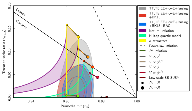
Figure 1: Marginalized joint $68\%$ and $95\%$ CL regions for $n_{s}$ and $r$ at $k=0.002\,Mpc^{-1}$ from Planck alone and in combination with BK15 or BK15+BAO data, compared to the theoretical predictions of selected inflationary models. This figure has been adapted from [5].

Choosing an arbitrary pivot scale $k_{\star}$ that exited the horizon, the scalar ($\mathcal{P}_{\zeta}$) and tensor ($\mathcal{P}_{T}$) power spectra can be written as

$$\mathcal{P}_{\zeta}(k)=A_{s}\left(\frac{k}{k_{\star}}\right)^{n_{s}-1},\qquad A_{s}\simeq\frac{1}{24\pi^{2}}\frac{V(\phi_{\star})}{\epsilon_{V}(\phi_{\star})}\qquad\mbox{and}\qquad\mathcal{P}_{T}(k)\simeq\frac{2V(\phi_{\star})}{3\pi^{2}}\left(\frac{k}{k_{\star}}\right)^{n_{t}}\,,$$ (1)

where the scale-dependence of the power spectra is defined by the scalar ($n_{s}$) and tensor ($n_{t}$) spectral indices given by

$$n_{s}-1=\frac{{\rm d}\ln\mathcal{P}_{\zeta}(k)}{{\rm d}\ln k}=-6\epsilon_{V}+2\eta_{V}\qquad\mbox{and}\qquad n_{t}=\frac{{\rm d}\ln\mathcal{P}_{T}(k)}{{\rm d}\ln k}\,.$$ (2)

In these we have used the potential slow-roll parameters (note that in most formulas we use $M_{\rm P}^{2}=1$ except when we want the dimensionality to be explicit)

$$\epsilon_{V}=\frac{1}{2}\left(\frac{V^{\prime}(\phi)}{V(\phi)}\right)^{2}\qquad\mbox{and}\qquad\eta_{V}=\frac{V^{\prime\prime}(\phi)}{V(\phi)}\,.$$ (3)

The tensor-to-scalar ratio is defined as

$$r=\frac{\mathcal{P}_{T}(k)}{\mathcal{P}_{\zeta}(k)}=16\epsilon_{V}.$$ (4)

The Planck collaboration [5] has set the following bounds on the values of the observables:

$$A_{s}=(2.10\pm 0.03)\times 10^{-9},\qquad n_{s}=0.9649\pm 0.0042\quad(1\sigma\mbox{ region}),\qquad r<0.056\,.$$ (5)

During inflation the variation of the scalar field is related to the so-called number of $e$-folds $N_{\star}$ which has to be between $50$ and $60$ for the horizon and flatness problems to be solved. Following [5, 6] the number of $e$-folds is given by

$$N_{\star}\simeq\int_{\phi_{\rm end}}^{\phi_{\star}}\frac{{\rm d}\phi}{\sqrt{2\epsilon_{V}}}=\ln\left[\left(\frac{\pi^{2}}{30}\right)^{\frac{1}{4}}\frac{(g_{s,0})^{\frac{1}{3}}}{\sqrt{3}}\frac{T_{0}}{H_{0}}\right]-\ln\left[\frac{k_{\star}}{a_{0}H_{0}}\right]+\frac{1}{4}\ln\left[\frac{V^{2}(\phi_{\star})}{\rho_{\rm end}}\right]-\frac{1}{12}\ln\left[g_{s,{\rm reh}}\right]\,,$$ (6)

where the subscripts $``0"$, $``{\rm reh}"$ and $``{\rm end}"$ denote quantities at the present epoch, at the reheating phase and at the end of inflation respectively. The energy density is denoted by $\rho$. The entropy density degrees of freedom (DOF) have the values $g_{s,0}=43/11$ and $g_{s,{\rm reh}}=\mathcal{O}(100)$ for $T_{\rm reh}\sim 1\,\mathrm{TeV}$ or higher. At the present epoch the CMB temperature and the Hubble constant are $T_{0}=2.725\,\mathrm{K}$ and $H_{0}=67.6\,\mathrm{km/s/Mpc}$ respectively and we fix the pivot scale to $k_{\star}=0.05\,\mbox{Mpc}^{-1}$ or $k_{\star}=0.002\,\mbox{Mpc}^{-1}$.

Starobinsky [7] and Higgs [8] inflation are two of the simplest and most successful models of inflation. In the Starobinsky model a $\mathcal{R}^{2}$ is added in the usual Einstein-Hilbert action which after a Weyl rescaling of the metric and a field redefinition is converted to a scalar DOF. If initially a scalar field is contained in the action, then two-field inflation takes place. In Higgs inflation a nonminimal coupling between gravity and the Higgs field $h$ is added in the action. The actions in the Jordan frame (JF) read

$$S_{JF}^{\rm S} = \int\mathrm{d}^{4}x\sqrt{-g}\left(\frac{M^{2}_{\rm Pl}\mathcal{R}}{2}+\frac{\mathcal{R}^{2}}{12M^{2}}\right)\,,$$ (7)

$$S_{JF}^{\rm H} = \int\mathrm{d}^{4}x\sqrt{-g}\left(\frac{(M^{2}_{\rm Pl}+\xi_{h}h^{2})\mathcal{R}}{2}-\frac{1}{2}(\partial h)^{2}-\frac{\lambda_{h}}{4}(h^{2}-v_{h}^{2})^{2}\right)\,,$$ (8)

while the corresponding EF inflationary potentials for the canonical normalized scalar fields are

$$\bar{U}^{\rm S}(\phi)=\frac{3M^{2}M^{4}_{\rm Pl}}{4}\left[1-\exp\left(-\sqrt{\frac{2}{3}}\frac{\phi}{M_{\rm Pl}}\right)\right]^{2}\,,\,\bar{U}^{\rm H}(\phi)=\frac{\lambda_{h}M^{4}_{\rm Pl}}{4\xi_{h}^{2}}\left(1+\exp\left(-\sqrt{\frac{2}{3}}\frac{\phi}{M_{\rm Pl}}\right)\right)^{-2}\,.$$ (9)

The parameters $M$ and $\xi_{h}$ are determined by the constraint on the amplitude of the scalar power spectrum. The rest cosmological observables are well within the allowed region in Fig. 1 as for both models $n_{s}=1-2/N_{\star}$ and $r=12/N_{\star}^{2}$.

2 Palatini formulation of gravity

In the context of Palatini gravity [9, 10], which is an interesting alternative to the usual metric theory of gravity, the metric tensor and the connection are treated as independent variables and one has to vary the action with respect to metric and the connection. In Palatini formulation the addition of higher order in curvature terms will not generate a propagating scalar DOF in the EF as in the metric case [11, 12, 13, 14, 15, 16, 17, 18, 19, 20, 21]. The differences between the formulations in the cosmological predictions, as far as inflation is concerned, arise from the nonminimal couplings of the scalars [22, 23, 24, 25, 26, 27, 28, 29, 30, 31, 32, 33, 34, 35, 36, 37, 38, 39, 40, 41, 42, 43, 44, 45, 46, 47, 48, 49, 50, 51, 52, 53, 54, 55, 56, 57, 58] or from higher order in curvature terms [59, 60, 61, 62, 63, 64, 65, 66, 67, 68, 69, 70, 71, 72, 73, 74, 75, 76, 77, 78, 79, 80, 81, 82] and has attracted the interest of many authors. Theories containing scale invariant quadratic terms in the context of metric formulation has recently received a lot of attention as a possible realization of quantum gravity [83, 84, 85, 86, 87, 88, 89, 90, 91, 92]. We will consider similar theories but in the Palatini case.

Starting from the JF Palatini action

$$S_{JF}=\int\mathrm{d}^{4}x\sqrt{-g}\left(\xi_{\phi}\phi^{2}\frac{R}{2}+\frac{\alpha}{2}R^{2}+\frac{\beta}{2}R_{(\mu\nu)}R^{(\mu\nu)}-\frac{1}{2}(\partial\phi)^{2}-V(\phi)\right)$$ (10)

and after a Weyl rescaling of the form $g_{\mu\nu}\rightarrow\Omega^{2}g_{\mu\nu}$ with $\Omega^{2}=\xi_{\phi}\phi^{2}$, we can pass to an intermediate frame (IF)

$$S_{IF}=\int\mathrm{d}^{4}x\sqrt{-g}\left(\frac{R}{2}+\frac{\alpha}{2}R^{2}+\frac{\beta}{2}R_{(\mu\nu)}R^{(\mu\nu)}-\frac{1}{2\Omega^{2}}(\partial\phi)^{2}-U(\phi)\right)\,,$$ (11)

with $U(\phi)=V(\phi)/\Omega^{4}$. Note also that the Planck scale is dynamically generated via the vacuum expectation value (VEV) of the scalar field as $M^{2}_{\rm Pl}=\xi_{\phi}v_{\phi}^{2}$. This is usually achieved in scale-invariant theories [93, 94, 95, 96, 97, 98, 99, 100, 101, 102, 87, 103, 104, 105, 106, 107, 108, 109, 110, 111, 112, 113, 114, 115, 91, 116, 45, 117, 118, 75, 76, 82], where the running of the inflaton quartic coupling induces symmetry breaking à la Coleman–Weinberg. Now, including an auxiliary field and after a conformal (or a disformal transformation [119, 120, 121, 122] in the $\beta\neq 0$ case), we obtain the final EF action

$$S_{EF}=\int\mathrm{d}^{4}x\sqrt{-g}\left(\frac{R}{2}-\frac{1}{2(1+\tilde{\alpha}U(s_{c}))}(\partial s_{c})^{2}-\bar{U}(s_{c})+\mathcal{O}\left((\partial s_{c})^{4}\right)\right)\,,$$ (12)

where $\tilde{\alpha}=2\beta+8\alpha$ and $s_{c}$ is the canonical field in the IF. The EF inflationary potential reads

$$\bar{U}(s_{c})=U(s_{c})/(1+\tilde{\alpha}U(s_{c}))\,.$$ (13)

The potential $\bar{U}(s_{c})$ reaches a plateau $1/\tilde{\alpha}$ for large field values. This flatness is quite capable to reduce the tensor-to-scalar ratio.

3 Nonminimal Coleman-Weinberg inflation in Palatini quadratic gravity

In [75] we considered the nonmimimal Coleman-Weinberg (CW) model [123] with a $R^{2}$ term $(\alpha\neq 0\,,\,\beta=0)$ in the Palatini formulation. The scalar potential contains a running quartic coupling $\lambda(\phi)$ and a cosmological constant $\Lambda$, that is

$$V(\phi)=\frac{1}{4}\lambda(\phi)\phi^{4}+\Lambda^{4}.$$ (14)

At the minimum we require that $V(v_{\phi})=0$, with $v^{2}_{\phi}=M^{2}_{\rm Pl}/\xi_{\phi}$. The minimization condition $\beta(v_{\phi})+4\lambda(v_{\phi})=0$ implies that, a) $\beta(v_{\phi})>0,\ \lambda(v_{\phi})<0$ or b) $\beta(v_{\phi})=\lambda(v_{\phi})=0$, where $\beta(v_{\phi})$ is the beta-function of the quartic coupling. Expanding the quartic coupling around the VEV and using the cases a) and b) we get that

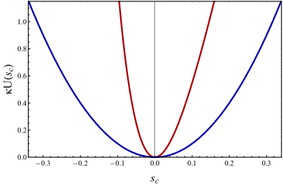
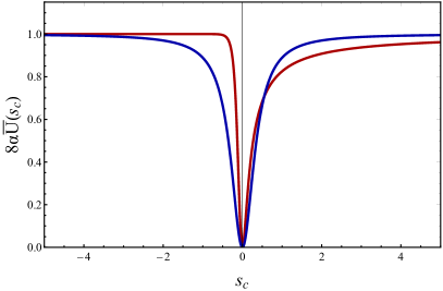
Figure 2: Left: Scalar potential $U(s_{c})$ of Eq.(17) for the 1st order CW model (red line) with $\kappa=\Lambda^{-4}$ and for the 2nd order CW model (blue line) with $\kappa=\xi_{\phi}^{2}/\beta^{\prime}$. Right: Scalar potential $\bar{U}(s_{c})$ of Eq.(13) for the 1st order CW model (red line) and for the 2nd order CW model (blue line).

$$\lambda^{a}(\phi)\simeq\lambda(v_{\phi})+\beta(v_{\phi})\ln\frac{\phi}{v_{\phi}}\,,\qquad\lambda^{b}(\phi)\simeq\frac{\beta^{\prime}(v_{\phi})}{2}\ln^{2}\frac{\phi}{v_{\phi}}\,,$$ (15)

which after substituting in (14) give the 1st and 2nd order JF CW potentials

$$V_{1}(\phi)=\Lambda^{4}\left\{1+\left[4\ln\left(\frac{\phi}{v_{\phi}}\right)-1\right]\frac{\phi^{4}}{v_{\phi}^{4}}\right\}\,,\qquad V_{2}(\phi)=\frac{1}{8}\beta^{\prime}\phi^{4}\ln^{2}\left(\frac{\phi}{v_{\phi}}\right)\,.$$ (16)

In the canonical normalized IF (11) the potentials (16) are of the form

$$U_{1}(s_{c})=\Lambda^{4}\left(4\sqrt{\xi_{\phi}}\frac{s_{c}}{M_{\rm Pl}}+e^{-4\sqrt{\xi_{\phi}}\frac{s_{c}}{M_{\rm Pl}}}-1\right)\,,\qquad U_{2}(s_{c})=\frac{\beta^{\prime}M^{2}_{\rm Pl}}{8\xi_{\phi}}s_{c}^{2}\,.$$ (17)

The 1st order potential behaves like a linear potential $U_{1}(s_{c})\propto s_{c}$ for $\xi_{\phi}\gg 1$ (and $s_{c}>0$) and as a quadratic potential $U_{1}(s_{c})\propto s_{c}^{2}$ for $\xi_{\phi}\ll 1$. The 2nd order is completely quadratic in the IF. Therefore the inflationary potential in the EF (12) after the effect of the $R^{2}$ term is given by (13) with $\tilde{\alpha}=8\alpha$. In Fig. 2 are displayed the IF potentials (17) (left) and the EF potentials (13) (right) for $\xi_{\phi}=10$, $\alpha=10^{10}$, $\beta^{\prime}=10^{-9}$ and $\Lambda=0.0015$. The normalized factor is $\kappa=\Lambda^{-4}$ or $k=\xi_{\phi}^{2}/\beta^{\prime}$ depending on the case. As is obvious the final EF inflationary potentials in the right panel are flat for large field values, approaching the plateau $1/8\alpha$.

Finally, in Fig. 3 we present the inflationary predictions for the 1st (left) and 2nd (right) order potentials, for various values of the parameter $\alpha$. For each curve, in the 1st order potential, the black dot corresponds to the $\xi_{\phi}\rightarrow 0$ limit. The parts of the curves in the left of the black dots correspond to small field inflation (SFI), while the right ones to large field inflation (LFI). The number of $e$-folds are predefined by Eq. (6) for $k_{\star}=0.05\,\mbox{Mpc}^{-1}$.

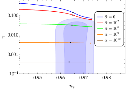
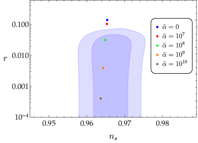
Figure 3: Left: The predictions for the tensor-to-scalar ratio ($r$) and the spectral index ($n_{\rm s}$) for the 1st order CW potential. Right: The predictions for the tensor-to-scalar ratio ($r$) and the spectral index ($n_{\rm s}$) for the 2nd order CW potential.

4 Scale invariant inflation with a $U(1)_{X}$ extension of the Standard Model in Palatini quadratic gravity

In [82] we considered a $U(1)_{X}$ extension of the Standard Model (SM) [124, 125, 126, 127, 128, 129, 130, 131] in which the extra particles are three right-handed (RH) neutrinos $N_{R}$, one gauge boson and one scalar field $\Phi$, which in the unitary gauge is given by $\Phi=(\phi+v_{\phi})/\sqrt{2}$. The relevant Lagrangians of the model are

$$\bullet \mathcal{L}^{\rm BSM}_{\rm Yukawa}=-y_{D}^{ij}\overline{\ell}^{i}_{L}HN^{j}_{R}-\frac{1}{2}y_{M}^{i}\Phi\overline{N}^{iC}_{R}N^{i}_{R}+h.c.\,,$$

$$\bullet \mathcal{L}^{\rm BSM}_{\rm scalar}=-\frac{1}{2}g^{\mu\nu}\partial_{\mu}\phi\partial_{\nu}\phi-\frac{1}{4}\lambda_{\phi}\phi^{4}+\frac{1}{4}\lambda_{h\phi}h^{2}\phi^{2}\,,$$

$$\bullet \mathcal{L}_{\rm SM}\qquad\mbox{with no Higgs mass term}\,,$$

$$\bullet \mathcal{L}_{\rm gravity}=\frac{1}{2}\left(\xi_{\phi}\phi^{2}+\xi_{h}h^{2}\right)g^{\mu\nu}R_{\mu\nu}+\frac{\alpha}{2}R^{2}+\frac{\beta}{2}R_{(\mu\nu)}R^{(\mu\nu)}\,.$$ (18)

The mass of the Higgs and the electroweak scale is generated through a portal coupling of the form $\lambda_{h\phi}h^{2}\phi^{2}$. Thus, the addition of the extra scalar field $\phi$ is necessary to preserve the scale invariance of our model since the known Higgs mass term contained in the SM Lagrangian is not scale invariant. Also, the Planck scale is dynamically generated when $\phi$ and $h$ develop their VEVs, that is $M^{2}_{\rm P}=\xi_{\phi}v_{\phi}^{2}+\xi_{h}v_{h}^{2}$.

The JF tree-level potential

$$V^{(0)}(\phi,h)=\frac{1}{4}\left(\lambda_{\phi}\phi^{4}-\lambda_{h\phi}h^{2}\phi^{2}+\lambda_{h}h^{4}\right)\,,$$ (19)

will be studied with the help of the Gildener-Weinberg formalism [132]. In this approach one first finds the flat direction (FD) of the tree-level potential and then computes the one-loop corrections only along this flat direction, since this is where the corrections play the dominant role. For reasons that will be clear later we will calculate the FD of the IF potential $U^{(0)}(\phi,h)=V^{(0)}(\phi,h)/\left(\xi_{\phi}\phi^{2}+\xi_{h}h^{2}\right)^{2}$. The FD is determined by the conditions $\partial_{\phi}U^{(0)}(\phi,h)=\partial_{h}U^{(0)}(\phi,h)=0$, which give that along the FD

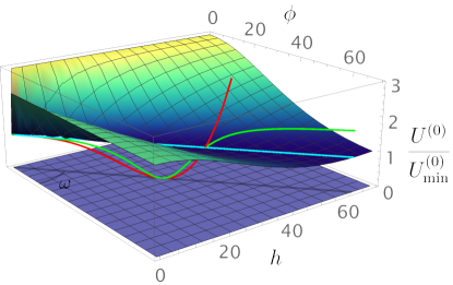
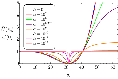
Figure 4: Left: The normalized tree-level potential $U^{(0)}(\phi,h)/U^{(0)}_{\rm min}$ and its flat direction (cyan line). The red curve corresponds to the normalized one-loop corrected IF potential along the flat direction $U_{\rm eff}(s_{c})/U_{\rm eff}(0)$, while the green one to the normalized EF potential $\bar{U}(s_{c})/\bar{U}(0)$. The values of the parameters are $\tilde{\alpha}=10^{9},\,\xi_{s}=0.001,\,$ and $\mathcal{M}\simeq 0.0357$. For illustrative purposes we have chosen the unrealistic value for the mixing angle $\omega\simeq 0.732$. Right: The normalized inflationary EF potential $\bar{U}(s_{c})$ for same $\xi_{s}\,,\,\mathcal{M}$ and various values of the parameter $\tilde{\alpha}$.

$$U^{(0)}_{\rm min}\equiv U^{(0)}(v_{\phi},v_{h})=\frac{\left(4\lambda_{h}\lambda_{\phi}-\lambda_{h\phi}^{2}\right)M^{4}_{\rm P}}{16\left[\lambda_{\phi}\xi_{h}^{2}+\xi_{\phi}\left(\lambda_{h\phi}\xi_{h}+\lambda_{h}\xi_{\phi}\right)\right]}\,.$$ (20)

In order to move from the initial frame of fields $\left(\phi,h\right)$ to the FD frame $\left(s,\sigma\right)$, where the direction of the so-called scalon field $s$ is identified with the FD and $\sigma$ is the perpendicular direction, we perform an orthogonal rotation described by the transformation

$$\left(\begin{array}[]{c}\phi\\ h\end{array}\right)=\begin{pmatrix}\cos{\omega}&-\sin{\omega}\\ \sin{\omega}&\cos{\omega}\end{pmatrix}\left(\begin{array}[]{c}s\\ \sigma\end{array}\right)\,,$$ (21)

where the mixing angle is given by $\omega=\arctan{\left(v_{h}/v_{\phi}\right)}$. Along the FD ($\sigma=0$) the only relevant DOF is the scalon $s$ which is related to $\phi$ and $h$ via $s^{2}=\phi^{2}+h^{2}$. As a consequence an effective nonminimal coupling constant is defined as $\xi_{s}=\xi_{\phi}\cos^{2}\omega+\xi_{h}\sin^{2}\omega$. Finally, we perform the following field redefinition in order to render the kinetic term of $s$ canonical:

$$s_{c}-v_{c}=\int_{v_{s}}^{s}\frac{1}{\sqrt{\xi_{s}}}\frac{{\rm d}s^{\prime}}{s^{\prime}}=\frac{1}{\sqrt{\xi_{s}}}\ln\frac{s}{v_{s}}\,.$$ (22)

The VEV $v_{s}$ of the scalon is related to the Planck mass with the familiar equation $v^{2}_{s}=M^{2}_{\rm P}/\xi_{s}$.

The one-loop corrections along the flat direction for the canonical field $s_{c}$ at the scale $\Lambda$ may be written as

$$U^{(1)}(s_{c})=\mathbb{A}\,s_{c}^{4}+\mathbb{B}\,s_{c}^{4}\ln\frac{s_{c}^{2}}{\Lambda^{2}}\,,$$ (23)

where in our model

$$\mathbb{A} = \frac{1}{64\pi^{2}v_{s}^{4}}\left\{M_{h}^{4}\left(\ln\frac{M_{h}^{2}}{v^{2}_{s}}-\frac{3}{2}\right)+6M_{W}^{4}\left(\ln\frac{M_{W}^{2}}{v^{2}_{s}}-\frac{5}{6}\right)+3M_{Z}^{4}\left(\ln\frac{M_{Z}^{2}}{v^{2}_{s}}-\frac{5}{6}\right)\right.$$ (24)

$$\left.\qquad\ +3M_{X}^{4}\left(\ln\frac{M_{X}^{2}}{v^{2}_{s}}-\frac{5}{6}\right)-6M_{N_{R}}^{4}\left(\ln\frac{M_{N_{R}}^{2}}{v^{2}_{s}}-1\right)-12M_{t}^{4}\left(\ln\frac{M_{t}^{2}}{v^{2}_{s}}-1\right)\right\}\,,$$

$$\mathbb{B} = \frac{\mathcal{M}^{4}}{64\pi^{2}v^{4}_{s}}\,,\qquad\mathcal{M}^{4}\equiv M_{h}^{4}+3M_{X}^{4}+6M_{W}^{4}+3M_{Z}^{4}-6M_{N_{R}}^{4}-12M_{t}^{4}\,.$$ (25)

Minimizing (23), we can determine the scale $\Lambda$ as $\Lambda=v_{s}\exp\left[\frac{\mathbb{A}}{2\mathbb{B}}+\frac{1}{4}\right]$. Then, the one-loop correction can be expressed as

$$U^{(1)}(s_{c})=\frac{\mathcal{M}^{4}}{64\pi^{2}v^{4}_{s}}s_{c}^{4}\left[\ln\frac{s_{c}^{2}}{v^{2}_{s}}-\frac{1}{2}\right]\,.$$ (26)

In order the potential (26) to be bounded from below, the parameter $\mathcal{M}^{4}$ must be positive. This is achieved if $3M_{X}^{4}-6M_{N_{R}}^{4}\gtrsim\left(317\ \rm GeV\right)^{4}$, where $M_{X}$ is the mass of the extra $U(1)_{X}$ gauge boson and $M_{N_{R}}$ are the RH neutrinos masses.

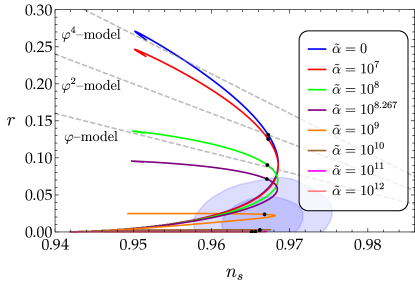
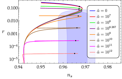
Figure 5: Left: The predictions for the tensor-to-scalar ratio ($r$) and the spectral index ($n_{\rm s}$) as $\xi_{s}$ ranges from $\xi_{s}\ll 1$ to $\xi_{s}\gg 1$ for various values of $\tilde{\alpha}$. For each curve, the black dot corresponds to the $\xi_{s}\rightarrow 0$ limit. Right: The same as the left, but in logarithmic scale.

Requiring that the full one-loop effective potential is zero at $v_{s}$, i.e. $U_{\rm eff}(v_{s})=U^{(0)}_{\rm min}+U^{(1)}(v_{s})=0$ we obtain that

$$U_{\rm eff}(s_{c})=\frac{\mathcal{M}^{4}}{128\pi^{2}}\left[\frac{s^{4}_{c}}{v^{4}_{s}}\left(2\ln\frac{s^{2}_{c}}{v^{2}_{s}}-1\right)+1\right]\,.$$ (27)

Note that we assume that $4\lambda_{h}\lambda_{\phi}-\lambda_{h\phi}^{2}>0$, so that $U^{(0)}_{\rm min}>0$. Had we opted to consider the one-loop corrections in the JF, and not in the IF, the extremization conditions for the tree-level JF potential would fix its value to zero along the flat direction and in conjunction with the fact that at the minimum the one-loop correction (26) is negative, the full one-loop effective potential would correspond to an anti-de Sitter vacuum.

Figure 4 illustrates the various potentials in the different frames of the model. As it is shown in the right panel, in the limit $\tilde{\alpha}\gg 1$ the potential becomes symmetric around its VEV and consequently the predictions for LFI and SFI are identical. This is also visible from Fig. 5, as the upper parts of the curves (LFI) coincide to the lower parts (SFI) as the parameter $\tilde{\alpha}$ becomes larger. In this figure the pivot scale $k_{\star}=0.002\,\mbox{Mpc}^{-1}$ has been used in order to determine the number of $e$-folds from Eq. (6), but the amplitude of the scalar power spectrum is fixed to $2.1\times 10^{-9}$ at the scale $k_{\star}=0.05\,\mbox{Mpc}^{-1}$. Finally, we have seen that for viable inflation $\xi_{s}\lesssim 4\times 10^{-3}$, which in turn implies a lower cutoff, $v_{s}\gtrsim 15\,M_{\rm P}$.

5 Conclusions

In conclusion, in the Palatini formulation, the higher order in curvature terms provide us an effective potential which is asymptotically flat for large field values, and as a consequence the tensor-to-scalar ratio can be significantly reduced. The Planck scale can be dynamically generated through the VEVs of the scalar fields, because of the terms $\xi_{i}\phi_{i}^{2}R$ containing in the action. The Higgs mass and the electroweak scale is generated through a possible portal coupling of the form $\lambda_{h\phi}h^{2}\phi^{2}$.

The research of IDG is co-financed by Greece and the European Union (European Social Fund- ESF) through the Operational Programme “Human Resources Development, Education and Lifelong Learning” in the context of the project “Strengthening Human Resources Research Potential via Doctorate Research - 2nd Cycle” (MIS-5000432), implemented by the State Scholarships Foundation (IKY). This work was supported by the Estonian Research Council grants MOBJD381, MOBTT5, MOBTT86 and PRG1055 and by the EU through the European Regional Development Fund CoE program TK133 “The Dark Side of the Universe”. TDP acknowledges the support of the grant 19-03950S of Czech Science Foundation (GAČR). The research work of VCS was supported by the Hellenic Foundation for Research and Innovation (H.F.R.I.) under the “First Call for H.F.R.I. Research Projects to support Faculty members and Researchers and the procurement of high-cost research equipment grant” (Project Number: 824).

References

References

- [1] Guth A H 1981 Phys. Rev. D23 347–356
- [2] Starobinsky A A 1982 Phys. Lett. 117B 175–178
- [3] Linde A D 1982 Phys. Lett. 108B 389–393
- [4] Albrecht A and Steinhardt P J 1982 Phys. Rev. Lett. 48 1220–1223
- [5] Akrami Y et al. (Planck) 2020 Astron. Astrophys. 641 A10 (Preprint 1807.06211)
- [6] Liddle A R and Leach S M 2003 Phys. Rev. D 68 103503 (Preprint astro-ph/0305263)
- [7] Starobinsky A A 1980 Phys. Lett. 91B 99–102
- [8] Bezrukov F L and Shaposhnikov M 2008 Phys. Lett. B659 703–706 (Preprint 0710.3755)
- [9] Palatini A 1919 Rendiconti del Circolo Matematico di Palermo (1884-1940) 43 203–212 ISSN 0009-725X
- [10] Ferraris M, Francaviglia M and Reina C 1982 General Relativity and Gravitation 14 243–254 ISSN 1572-9532
- [11] Kaiser D I and Sfakianakis E I 2014 Phys. Rev. Lett. 112 011302 (Preprint 1304.0363)
- [12] Kaneda S and Ketov S V 2016 Eur. Phys. J. C 76 26 (Preprint 1510.03524)
- [13] Myrzakulov R, Sebastiani L and Vagnozzi S 2015 Eur. Phys. J. C 75 444 (Preprint 1504.07984)
- [14] Odintsov S D and Oikonomou V K 2016 Phys. Rev. D94 124026 (Preprint 1612.01126)
- [15] Ema Y 2017 Phys. Lett. B 770 403–411 (Preprint 1701.07665)
- [16] Mori T, Kohri K and White J 2017 JCAP 10 044 (Preprint 1705.05638)
- [17] He M, Starobinsky A A and Yokoyama J 2018 JCAP 05 064 (Preprint 1804.00409)
- [18] Gundhi A and Steinwachs C F 2020 Nucl. Phys. B 954 114989 (Preprint 1810.10546)
- [19] Elizalde E, Odintsov S, Oikonomou V and Paul T 2019 JCAP 02 017 (Preprint 1810.07711)
- [20] He M, Jinno R, Kamada K, Park S C, Starobinsky A A and Yokoyama J 2019 Phys. Lett. B 791 36–42 (Preprint 1812.10099)
- [21] Canko D D, Gialamas I D and Kodaxis G P 2020 Eur. Phys. J. C 80 458 (Preprint 1901.06296)
- [22] Bauer F and Demir D A 2008 Phys. Lett. B 665 222–226 (Preprint 0803.2664)
- [23] Bauer F 2011 Gen. Rel. Grav. 43 1733–1757 (Preprint 1007.2546)
- [24] Tamanini N and Contaldi C R 2011 Phys. Rev. D 83 044018 (Preprint 1010.0689)
- [25] Bauer F and Demir D A 2011 Phys. Lett. B 698 425–429 (Preprint 1012.2900)
- [26] Rasanen S and Wahlman P 2017 JCAP 11 047 (Preprint 1709.07853)
- [27] Tenkanen T 2017 JCAP 12 001 (Preprint 1710.02758)
- [28] Racioppi A 2017 JCAP 12 041 (Preprint 1710.04853)
- [29] Markkanen T, Tenkanen T, Vaskonen V and Veermäe H 2018 JCAP 03 029 (Preprint 1712.04874)
- [30] Järv L, Racioppi A and Tenkanen T 2018 Phys. Rev. D 97 083513 (Preprint 1712.08471)
- [31] Fu C, Wu P and Yu H 2017 Phys. Rev. D 96 103542 (Preprint 1801.04089)
- [32] Racioppi A 2018 Phys. Rev. D 97 123514 (Preprint 1801.08810)
- [33] Carrilho P, Mulryne D, Ronayne J and Tenkanen T 2018 JCAP 06 032 (Preprint 1804.10489)
- [34] Kozak A and Borowiec A 2019 Eur. Phys. J. C 79 335 (Preprint 1808.05598)
- [35] Rasanen S and Tomberg E 2019 JCAP 01 038 (Preprint 1810.12608)
- [36] Rasanen S 2019 Open J. Astrophys. 2 (Preprint 1811.09514)
- [37] Almeida J P B, Bernal N, Rubio J and Tenkanen T 2019 JCAP 03 012 (Preprint 1811.09640)
- [38] Shimada K, Aoki K and Maeda K i 2019 Phys. Rev. D 99 104020 (Preprint 1812.03420)
- [39] Takahashi T and Tenkanen T 2019 JCAP 04 035 (Preprint 1812.08492)
- [40] Jinno R, Kaneta K, Oda K y and Park S C 2019 Phys. Lett. B 791 396–402 (Preprint 1812.11077)
- [41] Rubio J and Tomberg E S 2019 JCAP 04 021 (Preprint 1902.10148)
- [42] Bostan N 2020 Phys. Lett. B 811 135954 (Preprint 1907.13235)
- [43] Bostan N 2020 Commun. Theor. Phys. 72 085401 (Preprint 1908.09674)
- [44] Tenkanen T and Visinelli L 2019 JCAP 08 033 (Preprint 1906.11837)
- [45] Racioppi A 2021 JHEP 21 011 (Preprint 1912.10038)
- [46] Tenkanen T 2020 Gen. Rel. Grav. 52 33 (Preprint 2001.10135)
- [47] Borowiec A and Kozak A 2020 JCAP 07 003 (Preprint 2003.02741)
- [48] Järv L, Karam A, Kozak A, Lykkas A, Racioppi A and Saal M 2020 Phys. Rev. D 102 044029 (Preprint 2005.14571)
- [49] Karam A, Raidal M and Tomberg E 2021 JCAP 03 064 (Preprint 2007.03484)
- [50] McDonald J 2021 JCAP 04 069 (Preprint 2007.04111)
- [51] Gialamas I D, Karam A, Lykkas A and Pappas T D 2020 Phys. Rev. D 102 063522 (Preprint 2008.06371)
- [52] Verner S 2020 (Preprint 2010.11201)
- [53] Enckell V M, Nurmi S, Räsänen S and Tomberg E 2021 JHEP 04 059 (Preprint 2012.03660)
- [54] Reyimuaji Y and Zhang X 2021 JCAP 03 059 (Preprint 2012.14248)
- [55] Karam A, Karamitsos S and Saal M 2021 (Preprint 2103.01182)
- [56] Mikura Y, Tada Y and Yokoyama S 2021 Phys. Rev. D 103 L101303 (Preprint 2103.13045)
- [57] Kubota M, Oda K Y, Shimada K and Yamaguchi M 2021 JCAP 03 006 (Preprint 2010.07867)
- [58] Sáez-Chillón Gómez D 2021 (Preprint 2103.16319)
- [59] Olmo G J 2011 Int. J. Mod. Phys. D 20 413–462 (Preprint 1101.3864)
- [60] Bombacigno F and Montani G 2019 Eur. Phys. J. C 79 405 (Preprint 1809.07563)
- [61] Enckell V M, Enqvist K, Rasanen S and Wahlman L P 2019 JCAP 02 022 (Preprint 1810.05536)
- [62] Antoniadis I, Karam A, Lykkas A and Tamvakis K 2018 JCAP 11 028 (Preprint 1810.10418)
- [63] Antoniadis I, Karam A, Lykkas A, Pappas T and Tamvakis K 2019 JCAP 03 005 (Preprint 1812.00847)
- [64] Tenkanen T 2019 Phys. Rev. D 99 063528 (Preprint 1901.01794)
- [65] Edery A and Nakayama Y 2019 Phys. Rev. D 99 124018 (Preprint 1902.07876)
- [66] Giovannini M 2019 Class. Quant. Grav. 36 235017 (Preprint 1905.06182)
- [67] Tenkanen T 2020 Phys. Rev. D 101 063517 (Preprint 1910.00521)
- [68] Gialamas I D and Lahanas A 2020 Phys. Rev. D 101 084007 (Preprint 1911.11513)
- [69] Antoniadis I, Karam A, Lykkas A, Pappas T and Tamvakis K 2020 PoS CORFU2019 073 (Preprint 1912.12757)
- [70] Tenkanen T and Tomberg E 2020 JCAP 04 050 (Preprint 2002.02420)
- [71] Lloyd-Stubbs A and McDonald J 2020 Phys. Rev. D 101 123515 (Preprint 2002.08324)
- [72] Antoniadis I, Lykkas A and Tamvakis K 2020 JCAP 04 033 (Preprint 2002.12681)
- [73] Ghilencea D M 2020 Eur. Phys. J. C 80 1147 (Preprint 2003.08516)
- [74] Das N and Panda S 2021 JCAP 05 019 (Preprint 2005.14054)
- [75] Gialamas I D, Karam A and Racioppi A 2020 JCAP 11 014 (Preprint 2006.09124)
- [76] Ghilencea D M 2021 Eur. Phys. J. C 81 510 (Preprint 2007.14733)
- [77] Bekov S, Myrzakulov K, Myrzakulov R and Gómez D S C 2020 Symmetry 12 1958 (Preprint 2010.12360)
- [78] Dimopoulos K and Sánchez López S 2021 Phys. Rev. D 103 043533 (Preprint 2012.06831)
- [79] Gómez D S C 2021 Phys. Lett. B 814 136103 (Preprint 2011.11568)
- [80] Karam A, Tomberg E and Veermäe H 2021 JCAP 06 023 (Preprint 2102.02712)
- [81] Lykkas A and Tamvakis K 2021 (Preprint 2103.10136)
- [82] Gialamas I D, Karam A, Pappas T D and Spanos V C 2021 (Preprint 2104.04550)
- [83] Stelle K 1977 Phys. Rev. D 16 953–969
- [84] Biswas T, Mazumdar A and Siegel W 2006 JCAP 03 009 (Preprint hep-th/0508194)
- [85] Salvio A and Strumia A 2014 JHEP 06 080 (Preprint 1403.4226)
- [86] Edery A and Nakayama Y 2014 Phys. Rev. D 90 043007 (Preprint 1406.0060)
- [87] Farzinnia A and Kouwn S 2016 Phys. Rev. D 93 063528 (Preprint 1512.05890)
- [88] Salvio A and Strumia A 2018 Eur. Phys. J. C78 124 (Preprint 1705.03896)
- [89] Salvio A 2018 Front. in Phys. 6 77 (Preprint 1804.09944)
- [90] Edery A and Nakayama Y 2019 JHEP 11 169 (Preprint 1908.08778)
- [91] Ghilencea D 2019 JHEP 10 209 (Preprint 1906.11572)
- [92] Salvio A and Veermäe H 2020 JCAP 02 018 (Preprint 1912.13333)
- [93] Shaposhnikov M and Zenhausern D 2009 Phys. Lett. B671 187–192 (Preprint 0809.3395)
- [94] Garcia-Bellido J, Rubio J, Shaposhnikov M and Zenhausern D 2011 Phys. Rev. D 84 123504 (Preprint 1107.2163)
- [95] Khoze V V 2013 JHEP 1311 215 (Preprint 1308.6338)
- [96] Steele T G, Wang Z W, Contreras D and Mann R B 2014 Phys. Rev. Lett. 112 171602 (Preprint 1310.1960)
- [97] Ren J, Xianyu Z Z and He H J 2014 JCAP 06 032 (Preprint 1404.4627)
- [98] Kannike K, Racioppi A and Raidal M 2014 JHEP 1406 154 (Preprint 1405.3987)
- [99] Csaki C, Kaloper N, Serra J and Terning J 2014 Phys. Rev. Lett. 113 161302 (Preprint 1406.5192)
- [100] Kannike K, Hütsi G, Pizza L, Racioppi A, Raidal M et al. 2015 JHEP 1505 065 (Preprint 1502.01334)
- [101] Kannike K, Racioppi A and Raidal M 2016 JHEP 01 035 (Preprint 1509.05423)
- [102] Wang Z W, Steele T G, Hanif T and Mann R B 2016 JHEP 08 065 (Preprint 1510.04321)
- [103] Rinaldi M and Vanzo L 2016 Phys. Rev. D94 024009 (Preprint 1512.07186)
- [104] Marzola L, Racioppi A, Raidal M, Urban F R and Veermäe H 2016 JHEP 03 190 (Preprint 1512.09136)
- [105] Ferreira P G, Hill C T and Ross G G 2016 Phys. Lett. B 763 174–178 (Preprint 1603.05983)
- [106] Kannike K, Racioppi A and Raidal M 2017 Nucl. Phys. B918 162–177 (Preprint 1605.09378)
- [107] Marzola L and Racioppi A 2016 JCAP 1610 010 (Preprint 1606.06887)
- [108] Kannike K, Raidal M, Spethmann C and Veermäe H 2017 JHEP 04 026 (Preprint 1610.06571)
- [109] Ferreira P G, Hill C T and Ross G G 2017 Phys. Rev. D 95 043507 (Preprint 1610.09243)
- [110] Karam A, Pappas T and Tamvakis K 2017 Phys. Rev. D96 064036 (Preprint 1707.00984)
- [111] Karam A, Marzola L, Pappas T, Racioppi A and Tamvakis K 2018 JCAP 05 011 (Preprint 1711.09861)
- [112] Racioppi A 2018 Phys. Rev. D 97 123514 (Preprint 1801.08810)
- [113] Ferreira P G, Hill C T, Noller J and Ross G G 2018 Phys. Rev. D 97 123516 (Preprint 1802.06069)
- [114] Wetterich C 2019 (Preprint 1901.04741)
- [115] Vicentini S, Vanzo L and Rinaldi M 2019 Phys. Rev. D 99 103516 (Preprint 1902.04434)
- [116] Salvio A 2019 Eur. Phys. J. C 79 750 (Preprint 1907.00983)
- [117] Benisty D, Guendelman E, Nissimov E and Pacheva S 2020 Symmetry 12 481 (Preprint 2002.04110)
- [118] Tang Y and Wu Y L 2020 Phys. Lett. B 809 135716 (Preprint 2006.02811)
- [119] Bekenstein J D 1993 Phys. Rev. D 48 3641–3647 (Preprint gr-qc/9211017)
- [120] Zumalacárregui M and Garcia-Bellido J 2014 Phys. Rev. D 89 064046 (Preprint 1308.4685)
- [121] Afonso V I, Bejarano C, Beltran Jimenez J, Olmo G J and Orazi E 2017 Class. Quant. Grav. 34 235003 (Preprint 1705.03806)
- [122] Annala J 2020 (Preprint 2106.09438)
- [123] Coleman S R and Weinberg E J 1973 Phys.Rev. D7 1888–1910
- [124] Hempfling R 1996 Phys.Lett. B379 153–158 (Preprint hep-ph/9604278)
- [125] Chang W F, Ng J N and Wu J M S 2007 Phys. Rev. D 75 115016 (Preprint hep-ph/0701254)
- [126] Iso S, Okada N and Orikasa Y 2009 Phys.Lett. B676 81–87 (Preprint 0902.4050)
- [127] Englert C, Jaeckel J, Khoze V and Spannowsky M 2013 JHEP 1304 060 (Preprint 1301.4224)
- [128] Khoze V V and Ro G 2013 JHEP 1310 075 (Preprint 1307.3764)
- [129] Benic S and Radovcic B 2015 JHEP 01 143 (Preprint 1409.5776)
- [130] Das A, Okada N and Papapietro N 2017 Eur. Phys. J. C 77 122 (Preprint 1509.01466)
- [131] Marzo C, Marzola L and Vaskonen V 2019 Eur. Phys. J. C 79 601 (Preprint 1811.11169)
- [132] Gildener E and Weinberg S 1976 Phys. Rev. D 13 3333