Block Bregman Majorization Minimization with Extrapolation

Abstract

In this paper, we consider a class of nonsmooth nonconvex optimization problems whose objective is the sum of a block relative smooth function and a proper and lower semicontinuous block separable function. Although the analysis of block proximal gradient (BPG) methods for the class of block $L$-smooth functions have been successfully extended to Bregman BPG methods that deal with the class of block relative smooth functions, accelerated Bregman BPG methods are scarce and challenging to design. Taking our inspiration from Nesterov-type acceleration and the majorization-minimization scheme, we propose a block alternating Bregman Majorization-Minimization framework with Extrapolation (BMME). We prove subsequential convergence of BMME to a first-order stationary point under mild assumptions, and study its global convergence under stronger conditions. We illustrate the effectiveness of BMME on the penalized orthogonal nonnegative matrix factorization problem.

90C26, 49M37, 65K05, 15A23, 15A83

1 Introduction

In this paper, we consider the following nonsmooth nonconvex optimization problem

(1) $$\begin{split}\displaystyle\operatorname{minimize}_{\begin{subarray}{c}x=(x_{1},\ldots,x_{m})\end{subarray}}\quad&F(x):=f(x)+\sum_{i=1}^{m}g_{i}(x_{i})\\ \text{ subject to }\quad&x_{i}\in\mathcal{X}_{i}\text{ for }i=1,\ldots,m,\end{split}$$

where $\mathcal{X}_{i}$ is a closed convex set of a finite dimensional real linear space $\mathbb{E}_{i}$ for $i\in[m]:=\{1,2,\ldots,m\}$, $x$ can be decomposed into $m$ blocks $x=(x_{1},\ldots,x_{m})$ with $x_{i}\in\mathcal{X}_{i}$, $f$ is a continuously differentiable function, and $g_{i}$ is a proper and lower semicontinuous function (possibly with extended values), and $\mathcal{X}_{i}\cap\mathbf{dom}\,g_{i}\neq\emptyset$. We denote $\mathcal{X}:=\prod_{i=1}^{m}\mathcal{X}_{i}$. We assume $F$ is bounded from below throughout the paper.

1.1 Related works

The composite separable optimization problem (CSOP) (1) has been widely studied. It covers many applications including compressed sensing [7], sparse dictionary learning [1, 36], nonnegative tensor factorization [35, 19], and regularized sparse regression problems [11, 26]. When $f$ has the block Lipschitz smooth property (that is, for all $i\in[m]$ and fixing the values of $x_{j}$ for $j\neq i$, the block function $x_{i}\mapsto f(x)$ admits an $L_{i}$-Lipschitz continuous gradient), then the nonconvex CSOP can be efficiently solved by block proximal gradient (BPG) methods [10, 13, 32, 34]. These methods update each block $i$, while fixing the value of blocks $x_{j}$ for $j\neq i$, by minimizing over $x_{i}\in\mathcal{X}_{i}$ the block Lipschitz gradient surrogate function (see [20, Section 4]) as follows

(2) $$x_{i}^{k+1}\in\operatorname*{argmin}_{x_{i}\in\mathcal{X}_{i}}\left\langle{\nabla f_{i}^{k}(x_{i}^{k})},{x_{i}-x_{i}^{k}}\right\rangle+\frac{1}{2\gamma_{i}^{k}}\|x_{i}-x_{i}^{k}\|^{2}+g_{i}(x_{i}),$$

where $x_{i}^{k}$ is the value of block $i$ at iteration $k$, $f_{i}^{k}(\cdot)$ denotes the value of the block function $x_{i}\to f(x_{1}^{k+1},\ldots,x_{i-1}^{k+1},x_{i},x_{i+1}^{k},\ldots,x_{m}^{k})$, and $\gamma_{i}^{k}$ is a step-size. To accelerate the BPG methods, several inertial versions have been proposed, including

• the heavy ball type acceleration methods in [29] that calculate an extrapolation point $\bar{x}_{i}^{k}=x_{i}^{k}+\beta_{i}^{k}(x_{i}^{k}-x_{i}^{k-1})$, then solving (2) by replacing the proximal term $\frac{1}{2\gamma_{i}^{k}}\|x_{i}-x_{i}^{k}\|^{2}$ by $\frac{1}{2\gamma_{i}^{k}}\|x_{i}-\bar{x}_{i}^{k}\|^{2}$,

• the Nesterov-type acceleration methods in [35, 37] that takes the same step as the heavy ball acceleration but also replace $\nabla f_{i}^{k}(x_{i}^{k})$ in (2) by $\nabla f_{i}^{k}(\bar{x}_{i}^{k})$, and

• the acceleration methods using two extrapolation points in [19, 30] that evaluate the gradient $\nabla f_{i}^{k}$ in (2) at an extrapolation point different from $\bar{x}_{i}^{k}$.

These methods were proved to have convergence guarantees when solving the nonconvex CSOP. The analysis of BPG methods has been extended to Bregman BPG methods [3, 18, 33] that replace the proximal term $\frac{1}{2}\|x_{i}-x_{i}^{k}\|^{2}$ in (2) by a Bregman divergence $D_{\psi_{i}}(x_{i},x_{i}^{k})$ associated with a kernel function $\psi_{i}$ (see Definition 2.2) as follows

(3) $$\min_{x_{i}\in\mathcal{X}_{i}}\left\langle{\nabla f_{i}^{k}(x_{i}^{k})},{x_{i}-x_{i}^{k}}\right\rangle+\frac{1}{\gamma_{i}^{k}}D_{\psi_{i}}(x_{i},x_{i}^{k})+g_{i}(x_{i}).$$

The Bregman BPG methods can deal with a larger class of nonconvex CSOP in which the block function $x_{i}\mapsto f(x)$ may not have a $L_{i}$-Lipschitz continuous gradient, but is a relative smooth function (also known as a smooth adaptable function) [9, 22, 14]. Although the convergence analysis of BPG methods has been successfully extended to Bregman BPG methods, the convergence guarantees of their inertial versions for solving the nonconvex CSOP have not been studied much. In fact, to the best of our knowledge, there are only two papers addressing the convergence of inertial versions of Bregman BPG methods for solving (1), namely [2] and [20]. In [2], the authors consider an inertial Bregman BPG method that adds to $\nabla f_{i}^{k}(x_{i}^{k})$ in (3) a weak inertial force, $\alpha_{i}^{k}(x_{i}^{k}-x_{i}^{prev})$, where $\alpha_{i}^{k}$ is some extrapolation parameter and $x_{i}^{prev}$ is the previous value of $x_{i}^{k}$. In [20, Section 4.3], the authors introduce a heavy ball type acceleration with backtracking. The analysis of this method can be extended to a Nesterov-type acceleration with backtracking; however, the back-tracking procedure in [20, Section 4.3] for the Nesterov-type acceleration would be quite expensive since the computation of $f_{i}^{k}(\bar{x}_{i}^{k})$ and $\nabla f_{i}^{k}(\bar{x}_{i}^{k})$ would be required in the back-tracking process. Furthermore, there are no experiments in [2] and [20] to justify the efficacy of the inertial versions for Bregman BPG methods.

BPG and Bregman BPG methods belong to the block majorization minimization framework [20, 32] that updates one block $x_{i}$ of $x$ by minimizing a block surrogate function of the objective function. In [20, Section 6.2], the matrix completion problem (MCP), which also has the form of Problem (1), illustrates the advantage of using suitable block surrogate functions and the efficacy of TITAN, the inertial block majorization minimization framework proposed in [20]. Specifically, each subproblem that minimizes the block surrogate function used in TITAN has a closed-form solution while each proximal gradient step in the BPG method does not. Furthermore, TITAN outperforms BPG for the MCP. This motivates us to design an algorithm that allows using surrogate functions of $g_{i}$ to replace $g_{i}$, in contrast to the current Bregman BPG methods which do not change $g_{i}$ in the sub-problems; see (3).

1.2 Contribution and organization of the paper

After having introduced some preliminary notions of the Bregman distances and block relative smooth functions in Section 2, we propose in Section 3 a block alternating Bregman Majorization Minimization framework with Extrapolation (BMME) that uses Nesterov-type acceleration to solve Problem (1) in which $f$ is assumed to be a block relative smooth function with respect to $(\varphi_{1},\ldots,\varphi_{m})$; see Definition 2.4. This means that the gradient and the Bregman divergence in (3) are replaced with $\nabla f_{i}^{k}(\bar{x}_{i}^{k})$ and $D_{\varphi^{k}_{i}}(x_{i},\bar{x}_{i}^{k})$, respectively; see Algorithm 1. We use a line-search strategy proposed in [25] to determine the extrapolation point $\bar{x}_{i}^{k}$. We remark that the inertial Bregman BPG method proposed in [25], named CoCaIn, is for solving the CSOP with $m=1$ while BMME is for solving (1) with multiple blocks. Furthermore, CoCaIn requires its subproblem, which is Problem (3) with the gradient and the Bregman divergence being replaced by $\nabla f_{i}^{k}(\bar{x}_{i}^{k})$ and $D_{\varphi^{k}_{i}}(x_{i},\bar{x}_{i}^{k})$ (note that we can omit the index $i$ as $m=1$ for CoCaIn), to be solved exactly (in other words, to have a closed-form solution). This requirement would be restrictive in applications where the nonsmooth part $g_{i}$ is nonconvex and does not allow a closed form solution for the subproblem. In contrast, BMME employs surrogate functions for $g_{i}$, $i\in[m]$, that may lead to closed-form solutions for its subproblem, see an example in Appendix D. We note that CoCaIn requires $g_{i}(\cdot)+\alpha/2\|\cdot\|^{2}$ to be convex for some constant $\alpha\geq 0$ (see [25, Assumption C]) while BMME requires $x_{i}\mapsto u_{i}(x_{i},y_{i})$ to be convex for any $y_{i}\in\mathcal{X}_{i}$, where $u_{i}(\cdot,\cdot)$ is a surrogate function of $g_{i}$ (see Definition 3.1). And as such, our analysis may allow a larger class of $g_{i}$ than CoCaIn since $u_{i}$ with $u_{i}(x_{i},y_{i})=g_{i}(x_{i})+\alpha/2\|x_{i}-y_{i}\|^{2}$ is a surrogate function of $g_{i}$. It is important noting that the convexity assumption for the surrogate of $g_{i}$ allows BMME to use stepsizes that only depend on the relative smooth constants of $f$. In contrast, CoCaIn needs to start with an initial relative smooth constant that linearly depends on the value of $\alpha$ that makes $g_{i}(\cdot)+\alpha/2\|\cdot\|^{2}$ convex. This initial relative smooth constant could be very large and lead to a very small stepsizes which results in a slow convergence. To illustrate this fact, we provide an experiment in Appendix D to compare the performance of BMME and CoCaIn on the matrix completion problem.

In Section 4, we prove subsequential convergence of the sequence generated by BMME to a first-order stationary point of (1) under mild assumptions, and prove the global convergence under stronger conditions. Furthermore, the analysis in [25] does not consider the subsequential convergence but only proves the global convergence for $F$ satisfying the Kurdyka-Łojasiewicz (KL) property [21], and under the assumption that the domains of the kernel functions are the full space. In our convergence analysis, we assume that every limit point $x^{*}$ of the generated sequence by BMME satisfying the condition that $x_{i}^{*}$ lies in the interior of the domain of $x_{i}\mapsto\varphi_{i}(x_{1}^{*},\ldots,x_{i-1}^{*},x_{i},x_{i+1}^{*},x_{m}^{*})$ for $i\in[m]$. This assumption is naturally satisfied when the $\varphi_{i}$’s have a full domain or $\mathcal{X}\subset{\rm int\,dom\,}\varphi_{i}$. For example, the feasible set $\mathcal{X}=\{x:x_{i}\in\mathbb{R}^{d_{i}},x_{i}\geq\varepsilon>0\}$ (that is, each component of $x_{i}$ is lower bounded by a positive constant $\varepsilon$) and the Burg entropy $\varphi_{i}(x)=-\sum_{j=1}^{d_{i}}\log x_{ij}$ satisfy our assumption; see for example the perturbed Kullback-Leibler nonnegative matrix factorization in [18]. We then prove subsequential convergence without the assumption that $F$ satisfies the KL property, and prove global convergence with this assumption.

In Section 5, we apply BMME to solve a penalized orthogonal nonnegative matrix factorization problem (ONMF). We conclude the paper in Section 6.

2 Preliminaries: Bregman distances and relative smoothness

In this section, we present preliminaries of Bregman distances and relative smoothness. We adopt [14, Definition 2.1] to define a kernel generating distance which, for simplicity, we refer to as “kernel function”.

Definition 2.1 (Kernel generating distance).

Let $C$ be a nonempty, convex and open subset of $\mathbb{E}_{i}$. A function $\psi:\mathbb{E}_{i}\to\bar{\mathbb{R}}:=(-\infty,+\infty]$ associated with $C$ is called a kernel generating distance if it satisfies the following:

(i)

$\psi$ is proper, lower semicontinuous and convex with ${\rm dom\,}\psi\subset\bar{C}$, where $\bar{C}$ is the closure of $C$, and ${\rm dom\,}\partial\psi=C$.

(ii)

$\psi$ is continuously differentiable on ${\rm int\,dom\,}\psi\equiv C$.

Let us denote the class of kernel generating distances by $\mathcal{G}(C)$.

Definition 2.2.

Given $\psi\in\mathcal{G}(C)$, we define $D_{\psi}:{\rm dom\,}\psi\times{\rm int\,dom\,}\psi\to\mathbb{R}_{+}$ as the Bregman divergence associated with the kernel function $\psi$ as follows

$$D_{\psi}(x_{i},y_{i}):=\psi(x_{i})-\psi(y_{i})-\left\langle{\nabla\psi(y_{i})},{x_{i}-y_{i}}\right\rangle.$$

Definition 2.3 ($(L,l)$-relative smooth function).

Given $\psi\in\mathcal{G}(C)$, let $\phi:\mathbb{E}_{i}\to(-\infty,+\infty]$ be a proper and lower semicontinuous function with ${\rm dom\,}\psi\subset{\rm dom\,}\phi$, which is continuously differentiable on $C={\rm int\,dom\,}\psi$. We say $\phi$ is $(L,l)$-relative smooth to $\psi$ if there exist $L>0$ and $l\geq 0$ such that for any $x_{i},y_{i}\in C$,

(4) $$\phi(x_{i})-\phi(y_{i})-\left\langle{\nabla\phi(y_{i})},{x_{i}-y_{i}}\right\rangle\leq LD_{\psi}(x_{i},y_{i}),$$

and

(5) $$-lD_{\psi}(x_{i},y_{i})\leq\phi(x_{i})-\phi(y_{i})-\left\langle{\nabla\phi(y_{i})},{x_{i}-y_{i}}\right\rangle.$$

Whenever $\phi$ is convex, we may take $l=0$ and Definition 2.3 recovers [22, Definition 1.1]. In the case $l=L$, Definition 2.3 recovers [14, Definition 2.2].

Given a function $f:\mathbb{E}\to(-\infty,+\infty]$, for each $i\in[m]$ and any fixed $y_{j}$ for $j\neq i$, we define a block function $f(\cdot,y_{\neq i}):\mathbb{E}_{i}\to(-\infty,+\infty]$ by

(6) $$x_{i}\mapsto f(x_{i},y_{\neq i}):=f(y_{1},\ldots,y_{i-1},x_{i},y_{i+1},\ldots,y_{m}).$$

Definition 2.4 (Block relative smooth function).

We say that $f:\mathbb{E}\to(-\infty,+\infty]$ is a block relative smooth function with respect to $(\varphi_{1},\ldots,\varphi_{m})$, where $f$ is continuously differentiable on $\mathcal{C}={\rm int\,dom\,}\varphi_{1}=\cdots={\rm int\,dom\,}\varphi_{m}$ and ${\rm dom\,}\varphi_{1}=\ldots={\rm dom\,}\varphi_{m}\subset{\rm dom\,}f$, if, for any $y\in{\rm dom\,}\varphi_{i}$ we have $\varphi_{i}(\cdot,y_{\neq i})$ is a kernel generating function and the function $f(\cdot,y_{\neq i})$ is a $(L^{y_{\neq i}}_{i},l^{y_{\neq i}}_{i})$-relative smooth to $\varphi_{i}(\cdot,y_{\neq i})$, where $(L^{y_{\neq i}}_{i},l^{y_{\neq i}}_{i})$ may depend on $y_{j}$, $j\neq i$.

Throughout this paper we will assume the following.

Assumption 1.

We suppose $\mathcal{C}=\mathbf{int}\,\,\mathbf{dom}\,\varphi_{1}=\cdots=\mathbf{int}\,\,\mathbf{dom}\,\varphi_{m}$, $\mathbf{dom}\,\varphi_{1}=\ldots=\mathbf{dom}\,\varphi_{m}\subset\mathbf{dom}\,f$, $\mathcal{X}\cap\mathbf{dom}\,\varphi_{1}\neq\emptyset$, the function $f$ in (1) is a block relative smooth function with respect to $(\varphi_{1},...,\varphi_{m})$.

Let us make an important remark regarding Definition 2.4.

Flexibility of Definition 2.4.

Let us consider the notion of block relative smoothness in Definition 2.4 without $l^{y_{\neq i}}_{i}$, that is, the condition (5) is discarded. Similar definitions have been considered in [3] and [2]. In [3], the authors first define a multi-block kernel function $\psi:\mathbb{E}_{1}\times\ldots\mathbb{\times}E_{m}\to\bar{\mathbb{R}}$ [3, Definition 3.1], and then define multi-block relative smoothness of $f$ with respect to this multi-block kernel function with the relative smooth constants $(L_{1},\ldots,L_{m})$ [3, Definition 3.4]. In [2], the authors define the block relative smoothness of $f$ with respect to $(\psi_{1},\ldots,\psi_{m})$, where $\psi_{i}:\mathbb{E}_{1}\times\ldots\mathbb{E}_{m}\to\bar{\mathbb{R}}$ is an $i$-th block kernel function [2, Definition 2.1], with the relative smooth constants $(L_{1},\ldots,L_{m})$ [2, Definition 2.2]. It is crucial to note that $L_{1},\ldots,L_{m}$ in these definitions are constants and the stepsize used in the algorithms proposed in [3] and [2] to update each block $i$ is strictly less than $1/L_{i}$. In contrast, our Definition 2.4 allows the block $i$ relative smooth constant to change in the iterative process, that is, $L_{i}^{y_{\neq i}}$ and $l_{i}^{y_{\neq i}}$ are not constants but vary with respect to the values of the other blocks $y_{j}$ for $j\neq i$. This flexibility in Definition 2.4 will lead to more flexible choices for the block kernel functions, and also leads to variable step-sizes in designing Bregman BPG algorithms for solving the multi-block CSOP. In fact, as we will see in Algorithm 1, the stepsize to update block $i$ is $1/L_{i}^{k}$ which changes in the course of the iterative process. We will illustrate this crucial advantage of Algorithm 1 for solving the penalized ONMF problem in Section 5. Furthermore, it is important noting that if $f$ satisfies [2, Definition 2.1] or [3, Definition 3.4], then $f$ satisfies Definition 2.4 with the corresponding $L_{i}^{y_{\neq i}}$ being the constant $L_{i}$ for all $i\in[m]$. However, the converse does not hold; see an example in Section 5.1. Hence Algorithm 1 applies to a broader class of problems, while allowing a more flexible choice of the step-sizes which will lead to faster convergence; see Section 5.2.

3 Block Alternating Majorization Minimization with Extrapolation

Before introducing BMME, let us first recall the definition of a surrogate function as follows.

Definition 3.1.

A function $u_{i}:\mathcal{X}_{i}\times\mathcal{X}_{i}\to\bar{\mathbb{R}}$ is called a surrogate function of $g_{i}:\mathcal{X}_{i}\to\bar{\mathbb{R}}$ if the following conditions are satisfied:

(a)

$u_{i}(y_{i},y_{i})=g_{i}(y_{i})$ for all $y_{i}\in\mathcal{X}_{i}$,

(b)

$u_{i}(x_{i},y_{i})\geq g_{i}(x_{i})$ for all $x_{i},y_{i}\in\mathcal{X}_{i}$.

The approximation error is defined as $h_{i}(x_{i},y_{i}):=u_{i}(x_{i},y_{i})-g_{i}(x_{i})$.

For example, $u_{i}(x_{i},y_{i})=g_{i}(x_{i})+\frac{\alpha}{2}\|x_{i}-y_{i}\|^{2}$, where $\alpha$ is a nonnegative constant, is always a surrogate function of $g_{i}$. In this case, $h_{i}(x_{i},y_{i})=\frac{\alpha}{2}\|x_{i}-y_{i}\|^{2}$. We refer the readers to [20, 32, 23] for more examples.

Denote $x^{k,0}=x^{k}$ and

$$x^{k,i}=(x^{k+1}_{1},\ldots,x^{k+1}_{i},x^{k}_{i+1},\ldots,x^{k}_{m}).$$

For notation succinctness, we denote $\varphi_{i}^{k}(\cdot):=\varphi_{i}(\cdot,x^{k,i-1}_{\neq i})$, $L_{i}^{k}:=L_{i}^{x^{k,i-1}_{\neq i}}$, and $l_{i}^{k}:=l_{i}^{x^{k,i-1}_{\neq i}}$.

We can now introduce our BMME algorithm; see Algorithm 1. In particular, at iteration $k$, for each block $i$, BMME chooses a surrogate function $u_{i}$ of $g_{i}$ such that $x_{i}\mapsto u_{i}(x_{i},y_{i})$ is convex (as mentioned in the introduction, this condition is satisfied by the requirement that $g_{i}(\cdot)+\alpha/2\|\cdot\|^{2}$ is convex for some constant $\alpha\geq 0$ of [25]) and computes an extrapolated point $\bar{x}^{k}_{i}=x_{i}^{k}+\beta^{k}_{i}(x^{k}_{i}-x^{k-1}_{i})\in\mathbf{int}\,\,\mathbf{dom}\,\varphi_{i}^{k}$, where $\beta^{k}_{i}$ is an extrapolation parameter satisfying

$$D_{\varphi^{k}_{i}}(x^{k}_{i},\bar{x}^{k}_{i})\leq\frac{\delta_{i}L^{k-1}_{i}}{L^{k}_{i}+l^{k}_{i}}D_{\varphi^{k-1}_{i}}(x^{k-1}_{i},x^{k}_{i}),$$

for some $\delta_{i}\in(0,1)$. BMME then updates $x^{k,i}$ by

$$\begin{split}x^{k,i}_{i}&\in\operatorname*{argmin}_{x_{i}\in\mathcal{X}_{i}}\biggl{\{}L^{k}_{i}D_{\varphi^{k}_{i}}(x_{i},\bar{x}^{k}_{i})+\biggl{\langle}\nabla_{i}f(\bar{x}^{k}_{i},x^{k,i-1}_{\neq i}),x_{i}\biggr{\rangle}+u_{i}(x_{i},x_{i}^{k})\biggr{\}}\\ &=\operatorname*{argmin}_{x_{i}\in\mathbb{E}_{i}}\biggl{\{}L^{k}_{i}D_{\varphi^{k}_{i}}(x_{i},\bar{x}^{k}_{i})+\biggl{\langle}\nabla_{i}f(\bar{x}^{k}_{i},x^{k,i-1}_{\neq i}),x_{i}\biggr{\rangle}+\big{(}u_{i}(x_{i},x_{i}^{k})+I_{\mathcal{X}_{i}}(x_{i})\big{)}\biggr{\}},\end{split}$$

where $I_{\mathcal{X}_{i}}$ is the indicator function of $\mathcal{X}_{i}$. We make the following standard assumption for $\{x^{k}\}$, see for example [14, Assumption C]. Note that the initial points $x^{-1}$ and $x^{0}$ are chosen in the interior domain of $\varphi_{i}$, $i\in[m]$.

Assumption 2.

We have $x^{k}\in{\rm int\,dom\,}\varphi_{i}$, $i\in[m]$.

Assumption 2 is naturally satisfied when the domain of $\varphi_{i}$ is full space. See [14, Lemma 3.1] and  [14, Remark 3.1] for a sufficient condition that ensures (8) to produce $x_{i}^{k+1}\in\mathbf{int}\,\,\mathbf{dom}\,\varphi_{i}^{k}$, which implies that Assumption 2 holds.

Algorithm 1 BMME

1:  Choose $x^{-1},x^{0}\in{\rm int\,dom\,}\varphi_{i}$, $\delta_{i}\in(0,1)$, and set $k=0$. Let $u_{i}$ be a surrogate function of $g_{i}$ such that $x_{i}\mapsto u_{i}(x_{i},y_{i})$ is convex for any $y_{i}\in\mathcal{X}_{i}$.

2:  repeat

3:     for  $i=1,...,m$ do

4:        Compute an extrapolation parameter $\beta^{k}_{i}$ such that

(7) $$D_{\varphi^{k}_{i}}(x^{k}_{i},\bar{x}^{k}_{i})\leq\frac{\delta_{i}L^{k-1}_{i}}{L^{k}_{i}+l^{k}_{i}}D_{\varphi^{k-1}_{i}}(x^{k-1}_{i},x^{k}_{i}),$$

where $\bar{x}^{k}_{i}=x_{i}^{k}+\beta^{k}_{i}(x^{k}_{i}-x^{k-1}_{i})\in{\rm int\,dom\,}\varphi_{i}^{k}$.

5:        Update $x^{k,i}$ by

(8) $$\begin{split}x^{k+1}_{i}\in\operatorname*{argmin}_{x_{i}\in\mathcal{X}_{i}}\biggl{\{}L^{k}_{i}D_{\varphi^{k}_{i}}(x_{i},\bar{x}^{k}_{i})+\biggl{\langle}\nabla_{i}f(\bar{x}^{k}_{i},x^{k,i-1}_{\neq i}),x_{i}\biggr{\rangle}+u_{i}(x_{i},x_{i}^{k})\biggr{\}}.\end{split}$$

6:     end for

7:     $k\leftarrow k+1$.

8:  until Stopping criterion.

Choice of the extrapolation parameters.

BMME needs to adequately choose the extrapolation parameters $\beta^{k}_{i}$’s. Let us mention some special choices.

When $x_{i}\mapsto f(x_{i},y_{\neq i})$ admits an $L^{y_{\neq i}}_{i}$-Lipschitz continuous gradient, that is, $\varphi(\cdot,y_{\neq i})=\frac{1}{2}\|\cdot\|^{2}$, Condition (7) becomes

$$(\beta^{k}_{i})^{2}\|x^{k}_{i}-x^{k-1}_{i}\|^{2}\leq\frac{\delta_{i}L_{i}^{k-1}}{L_{i}^{k}+l_{i}^{k}}\|x^{k}_{i}-x^{k-1}_{i}\|^{2}.$$

Therefore, we can choose any $\beta^{k}_{i}$ such that $\beta^{k}_{i}\leq\sqrt{\frac{\delta_{i}L_{i}^{k-1}}{L_{i}^{k}+l_{i}^{k}}}$. Moreover, if $f(\cdot,y_{\neq i})$ is convex, we can take $l_{i}^{k}=0$ and hence we can choose any $\beta^{k}_{i}\leq\sqrt{\frac{\delta_{i}L_{i}^{k-1}}{L_{i}^{k}}}$.

In general, [25, Lemma 4.2] showed that if the symmetry coefficient of $\varphi_{i}^{k}$, which is defined by $\inf\Big{\{}\frac{D_{\varphi_{i}^{k}}(x_{i},y_{i})}{D_{\varphi_{i}^{k}}(y_{i},x_{i})}:x_{i},y_{i}\in\mathbf{int}\,\,\mathbf{dom}\,\varphi_{i}^{k}\Big{\}}$, is positive then, for a given

$$\kappa=\frac{\delta_{i}L^{k-1}_{i}}{L^{k}_{i}+l^{k}_{i}}D_{\varphi^{k-1}_{i}}(x^{k-1}_{i},x^{k}_{i})/D_{\varphi^{k}_{i}}(x^{k-1}_{i},x^{k}_{i})>0,$$

there always exists $\gamma^{k}_{i}>0$ such that the following condition is satisfied for all $\beta^{k}_{i}\in[0,\gamma_{i}^{k}]$

(9) $$D_{\varphi^{k}_{i}}(x^{k}_{i},\bar{x}^{k}_{i})\leq\kappa D_{\varphi^{k}_{i}}(x^{k-1}_{i},x^{k}_{i}),$$

which is equivalent to the condition (7). Therefore, $\beta_{i}^{k}$ can be determined by a line search as follows. At each iteration, we initialize $\beta_{i}^{k}=\frac{\nu_{i}^{k-1}-1}{\nu_{i}^{k}}$, where $\nu_{i}^{k}=\frac{1}{2}\left(1+\sqrt{1+4(\nu_{i}^{k-1})^{2}}\right)$ and $\nu_{i}^{0}=1$ as in Nesterov [27], and, while the inequality (7) does not hold, we decrease $\beta_{i}^{k}$ by a constant factor $\eta_{i}\in(0,1)$, that is, $\beta_{i}^{k}\leftarrow\beta_{i}^{k}\eta_{i}$.

Before proceeding to the convergence analysis, we make an important remark: the relative smoothness constants $L_{i}^{k}$ and $l_{i}^{k}$ in Algorithm 1 are assumed to be known at the moment of updating $x^{k}_{i}$. In case these values are unknown (or their known lower/upper bounds are too loose), we can employ the convex-concave backtracking strategy as in the algorithm CoCaIn BPG proposed in [25, Section 3.1] to determine these values as well as the extrapolation parameter $\beta_{i}^{k}$. The upcoming convergence analysis would be similar in that case. In Appendix D, we consider the matrix completion problem (MCP) which has the form of Problem (1) with $m=1$, and we illustrate BMME with the backtracking strategy on this problem when the values of the relative smooth constants are too small/large. The experiment presented in Appendix D on the MCP shows the backtracking strategy significantly improves the performance of BMME, and also outperforms CoCaIn BPG. However, to simplify the presentation, we will only consider the convergence analysis of BMME for solving the multi-block Problem (1) when the relative smooth constants are assumed to be known.

4 Convergence analysis

In this section, we study the subsequential convergence as well as the global convergence of BMME. For our upcoming analysis, we need the following first-order optimality condition of (1): $x^{*}$ is a first-order stationary point of (1) if

(10) $$\left\langle{p(x^{*})},{x-x^{*}}\right\rangle\geq 0\,\text{ for all }\,x\in\mathcal{X}\text{ and for some }\,p(x^{*})\in\partial F(x^{*}).$$

As $f$ is continuously differentiable folowing Assumption 1, $\partial F(x^{*})=\left\{\partial_{x_{1}}F(x^{*})\right\}\times\ldots\times\left\{\partial_{x_{m}}F(x^{*})\right\}$, where $\partial F(x^{*})$ is the limiting-subdifferential of $F$ at $x^{*}$, see Definition A.1 in Appendix A. Therefore, (10) is equivalent to

(11) $$\left\langle{p_{i}(x^{*})},{x_{i}-x_{i}^{*}}\right\rangle\geq 0\text{ for all }x_{i}\in\mathcal{X}_{i},\text{for some }p_{i}(x^{*})\in\partial_{x_{i}}F(x^{*})\text{ for }i\in[m].$$

If $x^{*}$ is in the interior of $\mathcal{X}$ or $\mathcal{X}_{i}=\mathbb{E}_{i}$ then (10) reduces to the condition $0\in\partial F(x^{*})$, that is, $x^{*}$ is a critical point of $F$.

4.1 Subsequential convergence

The following theorem presents the subsequential convergence of the sequence generated by Algorithm 1 under an additional assumption on the surrogate function of $g_{i}$.

Assumption 3.

• For $i\in[m]$, the surrogate function $u_{i}(\cdot,\cdot)$ of $g_{i}$ used in (8) in Algorithm 1 satisfies that $x_{i}\mapsto u_{i}(x_{i},y_{i})$ is convex.

• For $i\in[m]$, $u_{i}(x_{i},y_{i})$ is continuous in $y_{i}$ and lower semicontinuous in $x_{i}$.

• For $i\in[m]$, given $y_{i}\in\mathcal{X}_{i}$, there exists a function $x_{i}\mapsto\bar{h}_{i}(x_{i},y_{i})$ such that $\bar{h}_{i}(\cdot,y_{i})$ is continuously differentiable at $y_{i}$ and $\nabla_{x_{i}}\bar{h}_{i}(y_{i},y_{i})=0$, and the approximation error $x_{i}\mapsto h_{i}(x_{i},y_{i}):=u_{i}(x_{i},y_{i})-g_{i}(x_{i})$ satisfies

  (12) $$h_{i}(x_{i},y_{i})\leq\bar{h}_{i}(x_{i},y_{i})\;\text{ for all }\;x_{i}\in\mathcal{X}_{i}.$$

For example, if $g_{i}(\cdot)+\frac{\alpha}{2}\|\cdot\|^{2}$ is convex for some constant $\alpha\geq 0$ then the surrogate $u_{i}(x_{i},y_{i})=g_{i}(x_{i})+\frac{\alpha}{2}\|x_{i}-y_{i}\|^{2}$ satisfies Assumption 3 with $\bar{h}_{i}(x_{i},y_{i})=h_{i}(x_{i},y_{i})=\frac{\alpha}{2}\|x_{i}-y_{i}\|^{2}$. More examples can be found in [20].

Theorem 4.1.

Let $\{x^{k}\}$ be the sequence generated by Algorithm 1, and let Assumptions 1-3 be satisfied. The following statements hold.

• For $k=0,1,...$ we have

  (13) $$F(x^{k,i})\leq F(x^{k,i-1})-L^{k}_{i}D_{\varphi^{k}_{i}}(x^{k}_{i},x_{i}^{k+1})+\delta_{i}L^{k-1}_{i}D_{\varphi^{k-1}_{i}}(x_{i}^{k-1},x^{k}_{i}).$$

• If there exists a positive number $\underline{L}$ such that $\min_{k,i}L^{k}_{i}\geq\underline{L}$, we have

  (14) $$\sum_{k=0}^{+\infty}\sum_{i=1}^{m}D_{\varphi^{k}_{i}}(x_{i}^{k},x^{k+1}_{i})<+\infty.$$

• Assume that $\nabla_{x_{i}}\varphi_{i}(\cdot,y_{\neq i})$ for $i\in[m]$ is continuous in $y_{\neq i}$, $\{L_{i}^{k}\}$ for $i\in[m]$ and $\{x^{k}\}$ are bounded, and $\{\rho^{k}_{i}\}$ for $i\in[m]$ is bounded from below by $\rho>0$, where $\rho^{k}_{i}$ is the modulus of the strong convexity of $\varphi_{i}^{k}$. If $x^{*}$ is a limit point of $\{x^{k}\}$ and $x^{*}_{i}\in{\rm int\,dom\,}\varphi_{i}(\cdot,x_{\neq i}^{*})$, then $x^{*}$ is a first-order stationary point of Problem (1).

Proof 4.2.

A) Since $x^{k+1}_{i}$ is a solution to the convex problem (8), it follows from [28, Theorem 3.1.23] that for every $x_{i}\in\mathcal{X}_{i}$ we have

(15) $$\begin{split}\biggl{\langle}L^{k}_{i}(\nabla\varphi^{k}_{i}(x^{k+1}_{i})-\nabla\varphi^{k}_{i}(\bar{x}_{i}^{k}))+\nabla f(\bar{x}^{k}_{i},x^{k,i-1}_{\neq i}),x_{i}-x_{i}^{k+1}\biggr{\rangle}\\ +u_{i}(x_{i},x^{k}_{i})\geq u_{i}(x_{i}^{k+1},x^{k}_{i}).\end{split}$$

By choosing $x_{i}=x_{i}^{k}$, we obtain

(16) $$\begin{split}\biggl{\langle}L^{k}_{i}(\nabla\varphi^{k}_{i}(x^{k+1}_{i})-\nabla\varphi^{k}_{i}(\bar{x}_{i}^{k}))+\nabla f(\bar{x}^{k}_{i},x^{k,i-1}_{\neq i}),x_{i}^{k}-x_{i}^{k+1}\biggr{\rangle}\\ +u_{i}(x_{i}^{k},x^{k}_{i})\geq u_{i}(x_{i}^{k+1},x^{k}_{i}).\end{split}$$

Substituting $u_{i}(x_{i}^{k+1},x^{k}_{i})\geq g_{i}(x^{k+1}_{i})$ and $u_{i}(x_{i}^{k},x^{k}_{i})=g_{i}(x^{k}_{i})$ into this inequality gives

$$\begin{split}\biggl{\langle}L^{k}_{i}(\nabla\varphi^{k}_{i}(x^{k+1}_{i})-\nabla\varphi^{k}_{i}(\bar{x}_{i}^{k}))+\nabla f(\bar{x}^{k}_{i},x^{k,i-1}_{\neq i}),x_{i}^{k}-x_{i}^{k+1}\biggr{\rangle}+g_{i}(x^{k}_{i})\geq g_{i}(x^{k+1}_{i}).\end{split}$$

On the other hand, since $f$ is a block relative smooth function, we have

$$\begin{split}f(x^{k,i})\leq f(\bar{x}^{k}_{i},x^{k,i-1}_{\neq i})+\langle\nabla f(\bar{x}^{k}_{i},x^{k,i-1}_{\neq i}),x_{i}^{k+1}-\bar{x}^{k}_{i}\rangle+L^{k}_{i}D_{\varphi^{k}_{i}}(x_{i}^{k+1},\bar{x}^{k}_{i}),\end{split}$$

and

$$\begin{split}f(\bar{x}^{k}_{i},x^{k,i-1}_{\neq i})+\langle\nabla f(\bar{x}^{k}_{i},x^{k,i-1}_{\neq i}),x_{i}^{k}-\bar{x}^{k}_{i}\rangle\leq f(x^{k,i-1})+l^{k}_{i}D_{\varphi^{k}_{i}}(x_{i}^{k},\bar{x}^{k}_{i}),\end{split}$$

By summing the three inequalities above, we obtain

(17) $$\begin{split}F(x^{k,i})\leq F(x^{k,i-1})+L^{k}_{i}\biggl{\langle}\nabla\varphi^{k}_{i}(x^{k+1}_{i})-\nabla\varphi^{k}_{i}(\bar{x}_{i}^{k}),x_{i}^{k}-x_{i}^{k+1}\biggr{\rangle}\\ +L^{k}_{i}D_{\varphi^{k}_{i}}(x_{i}^{k+1},\bar{x}^{k}_{i})+l^{k}_{i}D_{\varphi^{k}_{i}}(x_{i}^{k},\bar{x}^{k}_{i}).\end{split}$$

Moreover, we have

(18) $$\begin{split}L^{k}_{i}\biggl{\langle}\nabla\varphi^{k}_{i}(x^{k+1}_{i})-\nabla\varphi^{k}_{i}(\bar{x}_{i}^{k}),x_{i}^{k}-x_{i}^{k+1}\biggr{\rangle}+L^{k}_{i}D_{\varphi^{k}_{i}}(x_{i}^{k+1},\bar{x}^{k}_{i})\\ =-L^{k}_{i}D_{\varphi^{k}_{i}}(x^{k}_{i},x_{i}^{k+1})+L^{k}_{i}D_{\varphi^{k}_{i}}(x_{i}^{k},\bar{x}^{k}_{i}),\end{split}$$

Therefore, we obtain

(19) $$\begin{split}F(x^{k,i})\leq F(x^{k,i-1})-L^{k}_{i}D_{\varphi^{k}_{i}}(x^{k}_{i},x_{i}^{k+1})+\biggl{(}L^{k}_{i}+l^{k}_{i}\biggr{)}D_{\varphi^{k}_{i}}(x_{i}^{k},\bar{x}^{k}_{i})\\ \leq F(x^{k,i-1})-L^{k}_{i}D_{\varphi^{k}_{i}}(x^{k}_{i},x_{i}^{k+1})+\delta_{i}L^{k-1}_{i}D_{\varphi^{k-1}_{i}}(x_{i}^{k-1},x^{k}_{i}),\end{split}$$

where the second inequality holds by (7). This implies A).

B) Summing (13) over $i=1,..,m$ gives

(20) $$F(x^{k+1})\leq F(x^{k})-\sum_{i=1}^{m}L^{k}_{i}D_{\varphi^{k}_{i}}(x^{k}_{i},x_{i}^{k+1})+\sum_{i=1}^{m}\delta_{i}L^{k-1}_{i}D_{\varphi^{k-1}_{i}}(x_{i}^{k-1},x^{k}_{i}).$$

By summing up this inequality from $k=0$ to $K-1$, we obtain

$$\begin{split}F(x^{K})+\sum_{i=1}^{m}\delta_{i}L^{K-1}_{i}D_{\varphi^{K-1}_{i}}(x_{i}^{K-1},x^{K}_{i})+\sum_{k=0}^{K-1}\sum_{i=1}^{m}(1-\delta_{i})L^{k}_{i}D_{\varphi^{k}_{i}}(x^{k}_{i},x_{i}^{k+1})\\ \leq F(x^{0})+\sum_{i=1}^{m}\delta L^{-1}_{i}D_{\varphi^{-1}_{i}}(x_{i}^{-1},x^{0}_{i}),\end{split}$$

which gives the result.

C) Let $x^{*}$ be a limit point of $\{x^{k}\}$. There exists a subsequence $\{x^{k_{n}}\}$ of $\{x^{k}\}$ converging to $x^{*}$. We have $D_{\varphi_{i}^{k}}(x_{i}^{k},x_{i}^{k+1})\geq\frac{\rho_{i}^{k}}{2}\|x_{i}^{k}-x_{i}^{k+1}\|^{2}$ since $\varphi_{i}^{k}$ is $\rho_{i}^{k}$-strongly convex. Together with the assumption $\rho_{i}^{k}\geq\rho>0$ and (14) we have $\|x^{k}-x^{k+1}\|$ converges to 0. Hence, $\{x^{k_{n}+1}\}$ and $\{x^{k_{n}-1}\}$ converge to $x^{*}$. Substituting $x_{i}=x^{*}_{i}$ and $k=k_{n}$ into (15) gives

(21) $$\begin{split}\biggl{\langle}L^{k_{n}}_{i}(\nabla\varphi^{k_{n}}_{i}(x^{k_{n}+1}_{i})-\nabla\varphi^{k_{n}}_{i}(\bar{x}_{i}^{k_{n}}))+\nabla f(\bar{x}^{k_{n}}_{i},x^{k_{n},i-1}_{\neq i}),x_{i}^{*}-x_{i}^{k_{n}+1}\biggr{\rangle}\\ +u_{i}(x_{i}^{*},x^{k_{n}}_{i})\geq u_{i}(x_{i}^{k_{n}+1},x^{k_{n}}_{i}).\end{split}$$

By taking $n\to+\infty$, we have

(22) $$\limsup_{n\to+\infty}u_{i}(x_{i}^{k_{n}+1},x^{k_{n}}_{i})\leq g_{i}(x_{i}^{*}),$$

where we have used the boundedness of $L^{k_{n}}_{i}$, the continuity of $u_{i}(x_{i},\cdot)$, $\nabla\varphi_{i}$, and $\nabla f$, $x^{*}_{i}\in{\rm int\,dom\,}\varphi_{i}(\cdot,x_{\neq i}^{*})$, and the fact that $x^{k_{n}+1}\to x^{*}$ as $n\to+\infty$. From this and the lower semi-continuity of $u_{i}(x_{i},y_{i})$, we have

(23) $$\lim_{n\to+\infty}u_{i}(x_{i}^{k_{n}+1},x^{k_{n}}_{i})=g_{i}(x_{i}^{*}).$$

Choosing $k=k_{n}$ in (15) and letting $n\to+\infty$ implies that, for all $x_{i}\in\mathcal{X}_{i}$,

(24) $$g_{i}(x^{*}_{i})\leq u_{i}(x_{i},x^{*}_{i})+\biggl{\langle}\nabla f(x^{*}_{i},x^{*}_{\neq i}),x_{i}-x_{i}^{*}\biggr{\rangle}.$$

Note that $u_{i}(x_{i},x^{*}_{i})=g_{i}(x_{i})+h_{i}(x_{i},x_{i}^{*})$ and $f(\cdot,x^{*}_{\neq i})$ is $(L_{i}^{*},l_{i}^{*})$-relative smooth to $\varphi_{i}^{*}(\cdot)=\varphi_{i}(\cdot,x^{*}_{\neq i})$ for some constant $L_{i}^{*},l_{i}^{*}$. Therefore, from (24) we have for all $x_{i}\in\mathcal{X}_{i}$ that

(25) $$\begin{split}F(x^{*})\leq F(x_{i},x^{*}_{\neq i})+l_{i}^{*}D_{\varphi^{*}_{i}}(x_{i},x^{*}_{i})+h_{i}(x_{i},x^{*}_{i})\\ \leq F(x_{i},x^{*}_{\neq i})+l_{i}^{*}D_{\varphi^{*}_{i}}(x_{i},x^{*}_{i})+\bar{h}_{i}(x_{i},x^{*}_{i}),\end{split}$$

where $\bar{h}_{i}$ satisfies Assumption B (3). This implies that $x^{*}_{i}$ is a minimizer of the following problem

(26) $$\min_{x_{i}\in\mathcal{X}_{i}}F(x_{i},x^{*}_{\neq i})+l_{i}^{*}D_{\varphi^{*}_{i}}(x_{i},x^{*}_{i})+\bar{h}_{i}(x_{i},x^{*}_{i}).$$

The result follows the optimality condition of (26) and $\nabla\bar{h}_{i}(x_{i}^{*},x^{*})=0$.

4.2 Global convergence

In order to prove the global convergence of Algorithm 1, we need to make an additional assumption.

Assumption 4.

For every iteration $k$ of Algorithm 1, $f(\cdot,x_{\neq i}^{k,i-1})$ is relative smooth with respect to $\varphi_{i}^{k}$ with constants $(L^{k}_{i},l_{i}^{k})$ for $i\in[m]$. We will assume the following:

(A)

There exist a positive integer number $N$, and $\underline{L}_{i},\bar{L}_{i}>0$ such that

• $\underline{L}_{i}\leq\min_{k\geq N}L^{k}_{i}\leq\max_{k\geq N}L^{k}_{i}\leq\bar{L}_{i}$ and $\delta_{i}<\underline{L}_{i}/\bar{L}_{i}$;

• for $i\in[m]$, $\varphi_{i}^{k}$ is $\rho_{i}^{k}$- strongly convex and there exists $\rho>0$ such that $\min_{k\geq N}\rho^{k}_{i}\geq\rho$.

(B)

$\nabla f$ and $\nabla\varphi_{i}$, for $i\in[m]$, are Lipschitz continuous on any bounded subsets of $\mathbb{E}$.

We remark that Assumption 4 (A) on the boundedness of $L_{i}^{k}$ is considered to be standard in the literature of inertial block coordinate methods, see [35, Assumption 2], [37, Assumption 2], [19, Assumption 3] for similar assumptions when considering block Lipschitz smooth problems. Assumptions 4 (B) is naturally satisfied when $f$ and $\varphi_{i}$ are twice continuously differentiable.

The global convergence of Algorithm 1 now can be stated for $F$ satisfying the KL property, see Definition A.3 in Appendix A.

Theorem 4.3.

Assume that Assumptions 1 to 4 hold. Let $\{x^{k}\}$ be the sequence generated by Algorithm 1. We further assume that (i) $\{x^{k}\}$ is bounded, (ii) for any $x_{i},y_{i}$ in a bounded subset of $\mathcal{X}_{i}$ if $s_{i}\in\partial_{x_{i}}(I_{\mathcal{X}_{i}}(x_{i})+u_{i}(x_{i},y_{i}))$, there exists $\xi_{i}\in\partial(I_{\mathcal{X}_{i}}(x_{i})+g_{i}(x_{i}))$ such that $\|\xi_{i}-s_{i}\|\leq A_{i}\|x_{i}-y_{i}\|$ for some constant $A_{i}$, and (iii) $F$ satisfies the KL property at any point $x^{*}\in\rm{dom\,}\partial F$. Then the whole sequence $\{x^{k}\}$ converges to a critical point $\Phi(x)=F(x)+\sum_{i=1}^{m}I_{\mathcal{X}_{i}}(x_{i})$.

Proof 4.4.

Consider the following auxiliary function

(27) $$\begin{split}&\Phi^{\gamma}(x,y)=\\ &\Phi(x)+\sum_{i=1}^{m}\gamma_{i}D_{\varphi_{i}}\big{(}(x_{1},\ldots,x_{i-1},y_{i},\ldots,y_{m}),(x_{1},\ldots,x_{i},y_{i+1},\ldots,y_{m})\big{)}\end{split}$$

where $\gamma_{i}=(\underline{L}_{i}+\delta_{i}\bar{L}_{i})/2$, and let us denote $z^{k}=(x^{k},x^{k-1})$. Then we have $\Phi^{\gamma}(z^{k})=\Phi(x^{k})+\sum_{i=1}^{m}\gamma_{i}D_{\varphi^{k-1}_{i}}(x^{k-1}_{i},x^{k}_{i})$. Here we only need to prove that the sequence $\{z^{k}\}$ satisfies the three conditions $\mathbf{H}1,\mathbf{H}2$, and $\mathbf{H}3$ in [8] since the result can be derived by using these conditions and the same arguments of the proof for [8, Theorem 2.9].

($\mathbf{H}1$) Sufficient decrease condition. It follows from (20) that for all $k\geq N+1$

(28) $$\sum_{i=1}^{m}\underline{L}_{i}D_{\varphi_{i}^{k}}(x^{k}_{i},x_{i}^{k+1})+F(x^{k+1})\leq F(x^{k})+\sum_{i=1}^{m}\delta_{i}\bar{L}_{i}D_{\varphi^{k-1}_{i}}(x_{i}^{k-1},x^{k}_{i}).$$

Therefore, we have

$$\begin{split}\Phi^{\gamma}(z^{k})-\Phi^{\gamma}(z^{k+1})&\geq\sum_{i=1}^{m}\frac{\underline{L}_{i}-\delta_{i}\bar{L}_{i}}{2}\biggl{(}D_{\varphi_{i}^{k-1}}(x_{i}^{k-1},x^{k}_{i})+D_{\varphi_{i}^{k}}(x^{k}_{i},x_{i}^{k+1})\biggr{)}\\ &\geq\sum_{i=1}^{m}\frac{(\underline{L}_{i}-\delta_{i}\bar{L}_{i})\rho_{i}}{4}\biggl{(}\|x_{i}^{k-1}-x^{k}_{i}\|^{2}+\|x^{k}_{i}-x_{i}^{k+1}\|^{2}\biggr{)}\\ &\geq\tau\|z^{k+1}-z^{k}\|^{2},\end{split}$$

where $\tau=\min_{i}(\underline{L}_{i}-\delta_{i}\bar{L}_{i})\rho_{i}/4>0$ due to Assumption 4.

($\mathbf{H}2$) Relative error condition. By using the optimal condition of the subproblem (8) in BMME, we have for all $k\geq N+1$

$$s_{i}^{k+1}:=L_{i}^{k}(\nabla\varphi^{k}_{i}(\bar{x}_{i}^{k})-\nabla\varphi_{i}^{k}(x_{i}^{k+1}))-\nabla_{i}f(\bar{x}_{i}^{k},x^{k,i-1}_{\neq i})\in\partial(I_{\mathcal{X}_{i}}(x_{i}^{k+1})+u_{i}(x_{i}^{k+1},x_{i}^{k})).$$

Hence, there exists $\xi_{i}^{k+1}\in\partial(I_{\mathcal{X}_{i}}(x_{i}^{k+1})+g_{i}(x^{k+1}_{i}))$ such that

(29) $$\|\xi_{i}^{k+1}-s_{i}^{k+1}\|\leq A_{i}\|x^{k+1}_{i}-x^{k}_{i}\|,$$

for some $A_{i}$. Therefore, we have $d^{k+1}_{i}:=\nabla_{x_{i}}f(x^{k+1})+\xi_{i}^{k+1}\in\partial_{x_{i}}\Phi(x^{k+1})$ and

$$\begin{split}\left\|d^{k+1}_{i}\right\|=\left\|\nabla_{x_{i}}f(x^{k+1})+s_{i}^{k+1}+\xi_{i}^{k+1}-s_{i}^{k+1}\right\|\leq\left\|L_{i}^{k}(\nabla\varphi^{k}_{i}(\bar{x}_{i}^{k})-\nabla\varphi^{k}_{i}(x_{i}^{k+1}))\right\|\\ +\left\|\nabla_{x_{i}}f(x^{k+1})-\nabla_{i}f(\bar{x}_{i}^{k},x^{k,i-1}_{\neq i})\right\|+\left\|\xi_{i}^{k+1}-s_{i}^{k+1}\right\|\\ \leq\left(\left(\bar{L}_{i}L^{\varphi_{i}}+L_{i}^{f}\right)\left(1+\beta_{i}^{k}\right)+A_{i}\right)\left(\left\|x^{k+1}_{i}-x^{k}_{i}\right\|+\left\|x^{k}_{i}-x^{k-1}_{i}\right\|\right),\end{split}$$

where the second inequality holds by (29), the boundedness of $\{x^{k}\}$, and the local Lipschitz continuity of $\nabla\varphi_{i}$ and $\nabla f$. On the other hand, $\partial\Phi^{\gamma}(z^{k+1})=\Big{(}\partial_{x}\Phi^{\gamma}(z^{k+1}),\partial_{y}\Phi^{\gamma}(z^{k+1})\Big{)}$, where

(30) $$\begin{split}\partial_{x_{i}}\Phi^{\gamma}(z^{k+1})&=\partial_{x_{i}}\Phi(x^{k+1})+\sum_{j=i+1}^{m}\gamma_{j}\big{(}\nabla_{i}\varphi_{j}(x^{k,j-1})-\nabla_{i}\varphi_{j}(x^{k,j})\big{)}\\ &\qquad-\sum_{j=i}^{m}\gamma_{j}\nabla^{2}_{ij}\varphi_{j}(x^{k,j})(x^{k}_{j}-x^{k+1}_{j})\end{split}$$

and

(31) $$\begin{split}\partial_{y_{i}}\Phi^{\gamma}(z^{k+1})&=\sum_{j=1}^{i-1}\gamma_{j}\big{(}\nabla_{i}\varphi_{j}(x^{k,j-1})-\nabla_{i}\varphi_{j}(x^{k,j})\big{)}-\sum_{j=1}^{i}\gamma_{j}\nabla^{2}_{ij}\varphi_{j}(x^{k,j})(x^{k}_{j}-x^{k+1}_{j}).\end{split}$$

Therefore, we can deduce the relative error condition from the results above.

($\mathbf{H}3$) Continuity condition. Let $x^{*}$ be a limit point of $\{x^{k}\}$. Since $\{x^{k}\}$ is bounded, there exists a subsequence $\{x^{k_{n}}\}$ of $\{x^{k}\}$ converging to $x^{*}$. Similarly to the proof of Theorem 4.1 (C), we can show that $u_{i}(x_{i}^{k_{n}},x^{k_{n}-1}_{i})\to g_{i}(x_{i}^{*})$ as $n\to+\infty$. Therefore, we have

(32) $$\begin{split}\limsup_{n\to+\infty}F(x^{k_{n}})\leq\limsup_{n\to+\infty}f(x^{k_{n}})+\sum_{i=1}^{m}u_{i}(x_{i}^{k_{n}},x^{k_{n}-1}_{i})\\ =f(x^{*})+\sum_{i=1}^{m}g_{i}(x^{*}_{i}).\end{split}$$

On the other hand, since $\{\Phi^{\gamma}(x^{k},x^{k-1})\}$ is non-increasing and bounded below, there exists $F^{*}=\lim_{k\to+\infty}\Phi^{\gamma}(x^{k},x^{k-1})$. Moreover, $\lim_{k\to+\infty}D_{\varphi^{k-1}_{i}}(x_{i}^{k-1},x^{k}_{i})=0$. This implies that $\lim_{k\to+\infty}F(x^{k})=\lim_{k\to+\infty}\Phi^{\gamma}(x^{k},x^{k-1})=F^{*}$. By the uniqueness of the limit, we have $F^{*}=F(x^{*})$.

By [8, Theorem 2.9] we have $z^{k}$ converges to a critical point $(x^{*},x^{*})$ of $\Phi^{\gamma}$. Note that $\partial\Phi^{\gamma}(x^{*},x^{*})=(\partial\Phi(x^{*}),0)$. The result follows then.

Convergence rate.

We end this section by a remark on the convergence rate of BMME. By using the same arguments of the proof for [6, Theorem 2] we can derive a convergence rate for the generated sequence of BMME (see also [2, Theorem 3.14], [3, Theorem 4.7], [19, Theorem 3] and [35, Theorem 2.9]). We note that the convergence rate appears to be the same in different papers using the technique in [6]. Specifically, suppose $\mathbf{a}$ be a constant such that $\xi(s)=cs^{1-\mathbf{a}}$, where $c$ is a constant, see Definition A.3. Then if $\mathbf{a}=0$, BMME converges after a finite number of steps; if $\mathbf{a}\in(0,1/2]$, BMME has linear convergence; and if $\mathbf{a}\in(1/2,1)$, BMME has sublinear convergence. Determining the KŁ exponent $\mathbf{a}$ is out of the scope of this paper.

5 Numerical results

In this section, we apply BMME to solve the following penalized orthogonal nonnegative matrix factorization (NMF) [3, 31]

(33) $$\min_{U\in\mathbb{R}_{+}^{\mathbf{m}\times\mathbf{r}},V\in\mathbb{R}_{+}^{\mathbf{r}\times\mathbf{n}}}f(U,V):=\tfrac{1}{2}\|X-UV\|_{F}^{2}+\tfrac{\lambda}{2}\|I_{r}-VV^{\top}\|_{F}^{2},$$

where $X\in\mathbb{R}^{\mathbf{m}\times\mathbf{n}}_{+}$ is a given input nonnegative data matrix and $\lambda>0$ is a penalty parameter. We implement all of the algorithms in MATLAB R2018a and run the experiments on a laptop with 1.8 GHz Intel Core i7 CPU and 16 GB RAM. The codes are available at https://github.com/LeThiKhanhHien/BMME.

5.1 Kernel functions and block updates of BMME

To implement BMME (Algorithm 1), we use the following kernel functions

(34) $$\begin{split}\varphi_{1}(U,V)&=\frac{1}{2}\|U\|_{F}^{2},\\ \varphi_{2}(U,V)&=\tfrac{6\lambda}{4}\|V\|_{F}^{4}+\tfrac{1}{2}\varepsilon(U)\|V\|_{F}^{2},\end{split}$$

where $\varepsilon(U)>0$ may depend on $U$. Let us choose $\varepsilon(U)=\max\{\|U^{\top}U\|,2\lambda\}$. Note that $U\mapsto\varphi_{1}(U,V)$ and $V\mapsto\varphi_{2}(U,V)$ are strongly convex. Let us show that $f$ is block relative smooth with respect to these kernel functions.

Proposition 5.1.

Fixing $V$, the function $f(\cdot,V)$ is $(L_{1}(V),l_{1})$-relatively smooth with respect to $\varphi_{1}(\cdot,V)$, with $L_{1}(V)=\|VV^{\top}\|$ and $l_{1}=0$. Fixing $U$, $f(U,\cdot)$ is $(L_{2},l_{2})$- relatively smooth with respect to $\varphi_{2}(U,\cdot)$, with $L_{2}=1$ and $l_{2}=1$.

Proof 5.2.

The first statement is straightforward. Let us prove the second one. From [3, Proposition 5.1], we have

$$\nabla_{V}^{2}f(U,V)[Z]=U^{\top}UZ+2\lambda(ZV^{\top}V+VZ^{\top}V+VV^{\top}Z-Z).$$

Note that

(35) $$\left|\left\langle{ZV^{\top}V+VZ^{\top}V+VV^{\top}Z},{Z}\right\rangle\right|\leq 3\|V\|_{F}^{2}\|Z\|_{F}^{2}.$$

Hence

$$\left\langle\nabla_{V}^{2}f(U,V)[Z],Z\right\rangle\leq\left\|U^{\top}U\right\|\left\|Z\right\|_{F}^{2}+6\lambda\left\|V\right\|_{F}^{2}\left\|Z\right\|_{F}^{2}.$$

Furthermore, we have

$$\nabla_{V}^{2}\varphi_{2}(U,V)[Z]=6\lambda\left(\|V\|_{F}^{2}Z+2\left\langle V,Z\right\rangle V\right)+\max\{\|U^{\top}U\|,\varepsilon\}Z,$$

which implies

$$L_{2}\left\langle\nabla_{V}^{2}\varphi_{2}(U,V)[Z],Z\right\rangle =\max\{\left\|U^{\top}U\right\|,2\lambda\}\left\|Z\right\|^{2}+6\lambda\left(\|V\|_{F}^{2}\left\|Z\right\|_{F}^{2}+2\left\langle V,Z\right\rangle^{2}\right)$$

$$\geq\left\|U^{\top}U\right\|\left\|Z\right\|_{F}^{2}+6\lambda\|V\|_{F}^{2}\left\|Z\right\|_{F}^{2}\geq\left\langle\nabla_{V}^{2}f(U,V)[Z],Z\right\rangle.$$

On the other hand, since $\max\{\|U^{\top}U\|,2\lambda\}\geq 2\lambda$ we have

$$\left\langle\nabla_{V}^{2}f(U,V)[Z],Z\right\rangle+l_{2}\left\langle\nabla_{V}^{2}\varphi_{2}(U,V)[Z],Z\right\rangle$$

$$\geq\left\langle U^{\top}UZ+2\lambda(ZV^{\top}V+VZ^{\top}V+VV^{\top}Z),Z\right\rangle+6\lambda\|V\|_{F}^{2}\|Z\|_{F}^{2}\geq 0,$$

where we have used (35) for the last inequality. The result follows, see [22, Proposition 1.1], [4, Proposition 2.6].

Proposition 5.1 shows that the kernel functions in (34) allow $f$ to satisfy Definition 2.4, that is, $f$ is block relative smooth with respect to these kernels. This would not hold for the block relative smoothness definitions from [2, Definition 2] and [3, Definition 3.4]. In fact, $L_{1}(V)$ depends on $V$ so [2, Definition 2] does not apply, while $\varphi_{1}$ and $\varphi_{2}$ are two different functions so [3, Definition 3.4] does not apply either as it requires a sole multi-block kernel function to define block relative smoothness.

In the following we provide closed-form solutions of the sub-problems in (8) for the penalized ONMF problem.

Proposition 5.3.

Let $\varphi_{1}$ and $\varphi_{2}$ be defined in (34). Given $\bar{U}$, $V$, and $L_{1}$, we have

$$\arg\min_{U\geq 0}\left\langle\nabla_{U}f(\bar{U},V),U\right\rangle+L_{1}D_{\varphi_{1}(\cdot,V)}(U,\bar{U})=\max\left(\bar{U}-\frac{1}{L_{1}}\left(\bar{U}VV^{\top}-XV^{\top}\right),0\right).$$

Given $\bar{V}$, $U$, and $L_{2}$ we have

$$\arg\min_{V\geq 0}\left\langle\nabla_{U}f(U,\bar{V}),V\right\rangle+L_{2}D_{\varphi_{2}(U,\cdot)}(V,\bar{V})\;=\;\frac{1}{\rho}\max(G(\bar{V}),0),$$

where

$$G(\bar{V}) =\nabla_{V}\varphi_{2}(U,\bar{V})-\frac{1}{L_{2}}\nabla_{V}f(U,\bar{V})$$

$$=(6\lambda\|\bar{V}\|^{2}_{F}+\varepsilon(U))\bar{V}-\frac{1}{L_{2}}\big{(}U^{\top}U\bar{V}-U^{\top}X+2\lambda(\bar{V}\bar{V}^{\top}\bar{V}-\bar{V})\big{)},$$

and $\rho$ is the unique real solution of the equation $\rho^{2}(\rho-a)=c$, where $a=\varepsilon(U)$ and $c=6\lambda\|\max(G(\bar{V}),0)\|^{2}$, so that $\rho$ has the following closed form

$$\rho=\frac{a}{3}+\sqrt[3]{\frac{c+\sqrt{\Delta}}{2}+\frac{a^{3}}{27}}+\sqrt[3]{\frac{c-\sqrt{\Delta}}{2}+\frac{a^{3}}{27}},$$

where $\Delta=c^{2}+\frac{4}{27}ca^{3}$.

Proof 5.4.

For the update of $U$, we have

$$\arg\min_{U\geq 0}\left\langle\nabla_{U}f(\bar{U},V),U\right\rangle+L_{1}D_{\varphi_{1}(\cdot,V)}(U,\bar{U})$$

$$=\arg\min_{U\geq 0}\left\langle\nabla_{U}f(\bar{U},V),U\right\rangle+L_{1}\left(\varphi_{1}(U,V)-\varphi_{1}(\bar{U},V)-\left\langle\nabla_{U}\varphi_{1}(\bar{U},V),U-\bar{U}\right\rangle\right)$$

$$=\arg\min_{U\geq 0}\varphi_{1}(U,V)-\left\langle\nabla_{U}\varphi_{1}(\bar{U},V)-\frac{1}{L_{1}}\nabla_{U}f(\bar{U},V),U\right\rangle$$

$$=\max\left(\nabla_{U}\varphi_{1}(\bar{U})-\frac{1}{L_{1}}\nabla_{U}f(\bar{U},V),0\right)$$

$$=\max\left(\bar{U}-\frac{1}{L_{1}}\left(\bar{U}VV^{\top}-XV^{\top}\right),0\right).$$

For the update of $V$, we have

$$\arg\min_{V\geq 0}\left\langle\nabla_{V}f(U,\bar{V}),V\right\rangle+L_{2}D_{\varphi_{2}(U,\cdot)}(V,\bar{V})$$

$$=\arg\min_{V\geq 0}\left\langle\nabla_{V}f(U,\bar{V}),V\right\rangle+L_{2}\left(\varphi_{2}(U,V)-\varphi_{2}(U,\bar{V})-\left\langle\nabla_{V}\varphi_{2}(U,\bar{V}),V\right\rangle\right)$$

$$=\arg\min_{V\geq 0}\varphi_{2}(U,V)-\left\langle G(\bar{V}),V\right\rangle.$$

Using the same technique as in the proof of [3, Theorem 5.2], we obtain the result.

Computational cost of BMME for Penalized ONMF

The updates of BMME for (33) are given by Proposition 5.3. The main cost of the update of $U$ is to compute $U(VV^{\top})$ and $XV^{\top}$ which require $O((\mathbf{m}+\mathbf{n})\mathbf{r}^{2})$ and $O(\mathbf{m}\mathbf{n}\mathbf{r})$ operations, respectively. Since $\mathbf{r}\ll\min(m,n)$, the update of $U$ costs $O(\mathbf{m}\mathbf{n}\mathbf{r})$ operations, and is linear in the dimensions of the input matrix, as most NMF algorithms. The main cost of the update of $V$ is to compute $(U^{\top}U)\bar{V}$, $U^{\top}X$, and $\bar{V}(\bar{V}^{\top}\bar{V})$ which require $O((\mathbf{m}+\mathbf{n})\mathbf{r}^{2})$, $O(\mathbf{m}\mathbf{n}\mathbf{r})$ and $O(\mathbf{n}\mathbf{r}^{2})$ operations, respectively. Evaluating $D(\cdot,\cdot)$ in the backtracking line search to compute the extrapolation parameter costs $O(\mathbf{n}\mathbf{r})$ operations. In summary, BMME requires $O(\mathbf{m}\mathbf{n}\mathbf{r})$ operations per iteration. Note that, if $X$ is sparse, the cost per iteration reduces to $O(\text{nnz}(X)\mathbf{r})$ operations where $\text{nnz}(X)$ is the number of nonzero entries of $X$.

In summary, BMME has the same computational cost per iteration as most NMF algorithms, requiring $O(\text{nnz}(X)\mathbf{r})$ operations per iteration, the main cost being the computation of $U(VV^{\top})$, $XV^{\top}$, $(U^{\top}U)V$, and $U^{\top}X$; see [15, Chapter 8] for a discussion.

5.2 Experiments on synthetic and real data sets

In the following, we compare the following algorithms on the penalized ONMF problem:

• BMME with the kernel functions defined in (34). At iteration $k$ and for updating the blocks $U$ and $V$, we find the extrapolation parameter $\beta_{i}^{k}$ for BMME by starting from $\nu_{k}$, where $\nu_{0}=1$ and $\nu_{k}=1/2(1+\sqrt{1+4\nu_{k-1}})$ for $k\geq 1$, and then reducing it by a factor $0.9$ until the condition (7) is satisfied.

• BMM, the non-extrapolated version of BMME.

• A-BPALM proposed in [3].

• BIBPA proposed in [2].

We use the kernel function $\varphi(U,V)=\frac{\alpha}{2}\|U\|_{F}^{2}\|V\|_{F}^{2}+\frac{\beta}{4}\|V\|_{F}^{4}+\frac{\varepsilon_{1}}{2}\|U\|_{F}^{2}+\frac{\varepsilon_{2}}{2}\|V\|_{F}^{2}$, where $\alpha,\beta,\varepsilon_{1}$ and $\varepsilon_{2}$ are positive constants, for A-BPALM and BIBPA as proposed in [3, Proposition 5.1], and choose the default values for the parameters of A-BPALM and BIBPA in the upcoming experiments. All of these algorithms have convergence guarantee for solving the penalized ONMF problem (33), and have roughly the same computational cost per iteration, requiring $O(\text{nnz}(X)\mathbf{r})$ operations. We will display the evolution of the objective function values with respect to time; the evolution with respect to the iterations being very similar.

In the following four sections, we compare the four algorithms above on four types of data sets: synthetic data sets (Section 5.2.1), facial images (Section 5.2.2), and document data sets (Section 5.2.3).

5.2.1 Synthetic data sets

Let us compare the algorithms on synthetic data sets, as done in [3]. We use $(\mathbf{m},\mathbf{n},\mathbf{r})=(500,500,10)$ and $(\mathbf{m},\mathbf{n},\mathbf{r})=(500,2000,10)$. For each choice of $(\mathbf{m},\mathbf{n},\mathbf{r})$, we generate 30 synthetic data sets; each data set is generated as in. Specifically, we generate randomly the factor $U\in\mathbb{R}_{+}^{\mathbf{m}\times\mathbf{r}}$ and the noise matrix $R\in\mathbb{R}_{+}^{\mathbf{m}\times\mathbf{n}}$ using the MATLAB command $\mathsf{rand}$. We generate an orthogonal nonnegative matrix $V\in\mathbb{R}_{+}^{\mathbf{r}\times\mathbf{n}}$ with a single nonzero entry in each column of $V$ as follows. The position of the nonzero entry is picked at random (with probability $1/r$ for each position), then the nonzero entry is generated using the uniform distribution in the interval $[0,1]$, and finally we normalize each row of $V$. Then we construct $X$, adding 5% of noise, as follows

$$X\;=\;UV+0.05\frac{\|X\|_{F}}{\|R\|_{F}}R.$$

For each data set, we run each algorithm for 15 seconds and use the same initialization for all algorithms, namely the successive projection algorithm (SPA) [5, 17] as done in [3]. We set the penalty parameter $\lambda=1000$ in our experiments. We report the evolution of the objective function with respect to time in Figure 1.

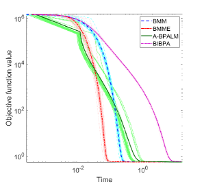
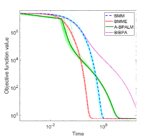
Figure 1: Evolution of the objective functions with respect to the running time for 30 synthetic data sets with $(\mathbf{m},\mathbf{n},\mathbf{r})=(500,500,10)$ (left) and $(\mathbf{m},\mathbf{n},\mathbf{r})=(500,2000,10)$ (right), in a log-log scale. The average curve is plotted in bold.

We observe that BMME consistently outperforms the other algorithms in term of convergence speed, followed by BMM and A-BPALM. Note that the results are very consistent among various runs on different input matrices.

These experiments illustrate two facts:

1. Using extrapolation in BMME is useful and accelerates the convergence, as BMME outperforms BMM.

2. The flexibility of Definition 2.4 allows BMME to choose the kernel functions in  (34) that also leads to a significant speedup as BMME outperforms A-BPALM and BIBPA. This illustrates our arguments in the paragraph “Flexibility of Definition 2.4” at the end of Section 2 (page 2).

In the next sections, we perform numerical experiments on real data sets to further validate these two key observations.

5.2.2 Facial images

In the second experiment, we compare the algorithms on four facial image data sets widely used in the NMF community: CBCL (2429 images of dimension 19 $\times$ 19), Frey (1965 images of dimension $28\times 20$), ORL (400 images of dimension $92\times 112$), and Umist (575 images of dimension $92\times 112$). We construct $X$ as an image-by-pixel matrix, that is, each row of $X$ is a vectorized facial image. As we will see, this allows ONMF to extract disjoint facial features as the rows of $V$. We set $\mathbf{r}=25$ and use SPA initialization in all runs. We choose the penalty parameter $\lambda=\|X-U_{0}V_{0}\|_{F}^{2}/\mathbf{r}$, where $(U_{0},V_{0})$ is the SPA initialization. We run each algorithm 100 seconds for each data set. The evolution of the scaled objective function values, which equal the objective function values divided by $\|X\|_{F}^{2}$, with respect to time is reported in Figure 2.

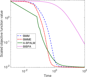
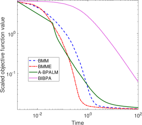
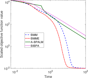
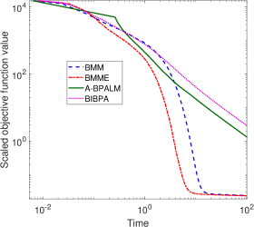
Figure 2: Evolution of the scaled objective function values with respect to running time on the CBCL (top left), Frey (top right), Umist (bottom left) and ORL (bottom right) data sets, in loglog scale.

We observe a similar behavior as for the synthetic data sets: BMME converges the fastest, followed by BMM. Figures 3 and 4 display the reshaped rows of $V$, corresponding to facial features, obtained by the different algorithms for the CBCL and ORL data sets, respectively. For the other data sets, Frey and Umist; see Appendix B.

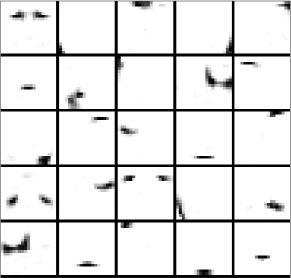
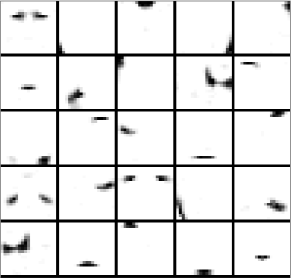
BMM	BMME
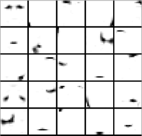
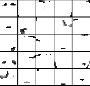
A-BPALM	BIBPA

Figure 3: Display of the rows of the matrix $V$ as facial features, computed by BMM, BMME, A-BPALM, and BIBPA on the CBCL facial images.

In Figure 3, we observe that the solutions obtained by the 4 algorithms are similar. Because BIBPA did not have time to converge (see Figure 2), it generates slightly worse facial features, with some isolated pixels, and edges of the facial features being sharper.

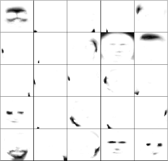
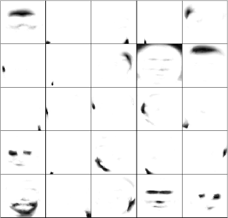
BMM	BMME
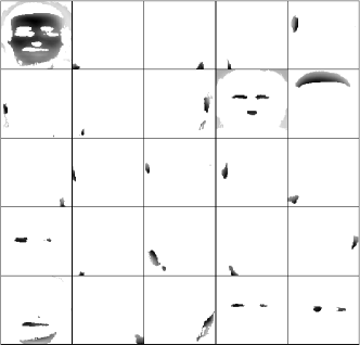
A-BPALM	BIBPA

Figure 4: Display of the rows of the matrix $V$ as facial features, computed by BMM, BMME, A-BPALM, and BIBPA on the ORL facial images.

In Figure 4, as BMM and BMME both converged to similar objective function values (see Figure 2), they provide very similar facial features; although slightly different. For example, the first facial feature of BMME is sparser than that of BMM. A-BPALM and BIBPA were not able to converge within the 100 seconds, and hence provide worse facial features. For example, the first facial feature is much denser than for BMM and BMME, overlapping with other facial features (meaning that the orthogonality constraints is not well satisfied). (A very similar observation holds for the Umist data set; see Appendix B.)

5.2.3 Document data sets

In the fourth experiment, we compare the algorithms on 12 sparse document data sets from [38], as in [31]. For such data sets, SPA does not provide a good initialization, because of outliers and gross corruptions. Hence we initialize $U_{0}$ with the procedure provided by H2NMF from [16], while $V_{0}$ is initialized by minimizing $\|X-U_{0}V_{0}\|_{F}^{2}$ while imposing $V_{0}$ to have a single nonzero entry per column. The penalty parameter $\lambda$ is chosen as before, namely $\lambda=\|X-U_{0}V_{0}\|_{F}^{2}/\mathbf{r}$. We run each algorithm 200 seconds for each data set. Table 1 reports the clustering accuracy obtained by the algorithms, which is defined as follows. Given the true clusters, $C_{k}$ for $k=1,2,\dots,\mathbf{r}$, and the clusters computed by an algorithm, $C^{\prime}_{k}$ for $k=1,2,\dots,\mathbf{r}$ (in ONMF, a data point is assigned to the cluster corresponding to the largest entry in the corresponding column of $V$), the accuracy of the algorithm is defined as

$$\text{Accuracy}\quad=\max_{\pi,\text{ a permutation of $[\mathbf{r}]$}}\frac{1}{\mathbf{n}}\left(\sum_{k=1}^{\mathbf{r}}\left|C_{k}\cap C^{\prime}_{\pi(k)}\right|\right).$$

Table 1: Accuracy in percent obtained by the different algorithms on 12 document data sets. The best accuracy is highlighted in bold.

Data set	rank $\mathbf{r}$	BMM	BMME	A-BPALM	BIBPA
hitech	6	39.94	39.93	38.98	37.07
reviews	5	73.56	73.53	66.70	66.31
sports	7	50.09	50.13	42.93	42.93
ohscal	10	31.70	31.52	27.25	27.25
la1	6	49.86	53.37	41.32	41.32
la2	6	53.43	52.46	54.83	50.34
classic	4	60.74	61.43	50.70	50.10
k1b	6	79.19	79.19	71.41	71.41
tr11	9	37.44	37.44	37.44	41.30
tr23	6	41.67	41.67	41.67	40.20
tr41	10	38.61	38.61	38.61	35.08
tr45	10	35.51	35.51	35.51	37.82
average		49.31	49.57	45.61	45.09

We observe on Table 1 that BMM and BMME provide, on average, better clustering accuracies than A-BPALM and BIBPA. In fact, in terms of accuracy, BMM performs similarly as BMME as both algorithms were able to converge within the allotted time (see Figure 5 and Appendix C). When A-BPALM or BIBPA have a better clustering accuracy, it is only by a small margin (less than 4% in all cases), while BMM and/or BMME sometimes outperform A-BPALM and BIBPA; in particular, by 6.8% for reviews, 7.2% for sports, 12% for la1, 10.7% for classic, and 7.8% for k1b.

The scaled objective function values with respect to time for the hitech and reviews data set are reported in Figure 5; the results for the other data sets are similar, and can be found in Appendix C. As before, BMME is the fastest, followed by BMM, A-BPALM and BIBPA (in that order).

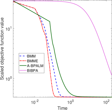
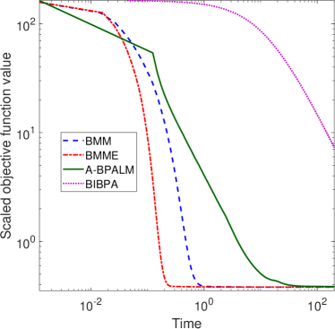
Figure 5: Evolution of the scaled objective function values with respect to running time on the hitech (left) and review (right) data sets, in loglog scale.

6 Conclusion

In this paper, we have developed BMME, a block alternating Bregman Majorization Minimization framework with Extrapolation that uses the Nesterov acceleration technique, for a class of nonsmooth nonconvex optimization problems that does not require the global Lipschitz gradient continuity. We have proved the subsequential and global convergence of BMME to first-order stationary points; see Theorems 4.1 and 4.3, respectively. We have evaluated the performance of BMME on the penalized orthogonal nonnegative matrix factorization problem on synthetic data sets, facial images, and documents. The numerical results have shown that (1) Using extrapolation improves the convergence of BMME, and (2) BMME converges faster than previously introduced the Bregman BPG methods, A-BPALM [3] and BIBPA [2], because BMME allows a much more flexible choice of the kernel functions and uses Nesterov-type extrapolation.

Appendix A Preliminaries of nonconvex nonsmooth optimization

Let $g:\mathbb{E}\to\mathbb{R}\cup\{+\infty\}$ be a proper lower semicontinuous function.

Definition A.1.

• For each $x\in{\rm dom}\,g,$ we denote $\hat{\partial}g(x)$ as the Frechet subdifferential of $g$ at $x$ which contains vectors $v\in\mathbb{E}$ satisfying

  $$\liminf_{y\neq x,y\to x}\frac{1}{\left\|y-x\right\|}\left(g(y)-g(x)-\left\langle v,y-x\right\rangle\right)\geq 0.$$

  If $x\not\in{\rm dom}\>g,$ then we set $\hat{\partial}g(x)=\emptyset.$

• The limiting-subdifferential $\partial g(x)$ of $g$ at $x\in{\rm dom}\>g$ is defined as follows.

  $$\partial g(x):=\left\{v\in\mathbb{E}:\exists x^{k}\to x,\,g\big{(}x^{k}\big{)}\to g(x),\,v^{k}\in\hat{\partial}g\big{(}x^{k}\big{)},\,v^{k}\to v\right\}.$$

Definition A.2.

We call $x^{*}\in\rm{dom}\,F$ a critical point of $F$ if $0\in\partial F\left(x^{*}\right).$

We note that if $x^{*}$ is a local minimizer of $F$ then $x^{*}$ is a critical point of $F$.

Definition A.3.

A function $\phi(x)$ is said to have the KL property at $\bar{x}\in{\rm dom}\,\partial\,\phi$ if there exists $\eta\in(0,+\infty]$, a neighborhood $U$ of $\bar{x}$ and a concave function $\xi:[0,\eta)\to\mathbb{R}_{+}$ that is continuously differentiable on $(0,\eta)$, continuous at $0$, $\xi(0)=0$, and $\xi^{\prime}(s)>0$ for all $s\in(0,\eta),$ such that for all $x\in U\cap[\phi(\bar{x})<\phi(x)<\phi(\bar{x})+\eta],$ we have

(36) $$\xi^{\prime}\left(\phi(x)-\phi(\bar{x})\right)\,\operatorname*{dist}\left(0,\partial\phi(x)\right)\geq 1.$$

$\operatorname*{dist}\left(0,\partial\phi(x)\right)=\min\left\{\|y\|:y\in\partial\phi(x)\right\}$. If $\phi(x)$ has the KL property at each point of ${\rm dom}\,\partial\phi$ then $\phi$ is a KL function.

Many nonconvex nonsmooth functions in practical applications belong to the class of KL functions, for examples, real analytic functions, semi-algebraic functions, and locally strongly convex functions [12, 13].

Appendix B Facial features extracted by the ONMF algorithms on the Frey and Umist facial images

Figures 6, and 7 display the facial features extracted by BMM, BMME, A-BPALM and BIBPA for the Frey and Umist facial images, respectively.

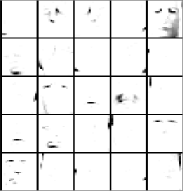
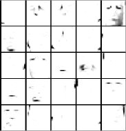
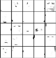
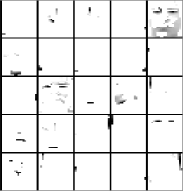
BMM	BMME	A-BPALM	BIBPA

Figure 6: Display of the rows of the matrix $V$ as facial features, computed by BMM, BMME, A-BPALM, and BIBPA on the Frey facial images.

In Figure 6, facial features are rather similar, although BMM and BMME obtained smaller objective function values.

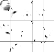
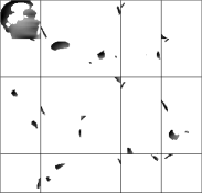
BMM	BMME	A-BPALM	BIBPA

Figure 7: Display of the rows of the matrix $V$ as facial features, computed by BMM, BMME, A-BPALM, and BIBPA on the Umist facial images.

In Figure 7, as BMM and BMME both converged to similar objective function values (see Figure 2), they provide very similar facial features. A-BPALM and BIBPA were not able to converge within the 100 seconds, and hence provide worse facial features. For example, the first facial feature is much denser than for BMM and BMME, overlapping with other facial features (meaning that the orthogonality constraints is not well satisfied).

Appendix C Scaled objective function values for document data sets

Figures 8 and 9 display the scaled objective function values for the document data sets on the penalized ONMF problem. We observe that, except for tr41 and tr45 where A-BPALM is able to compete with BMM and BMME, BMM and BMME outperform A-BPALM and BIBPA which performs particularly badly on these sparse data sets.

sports	ohscal
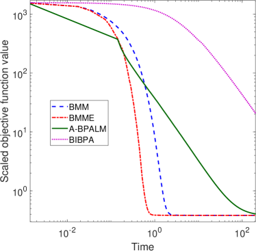
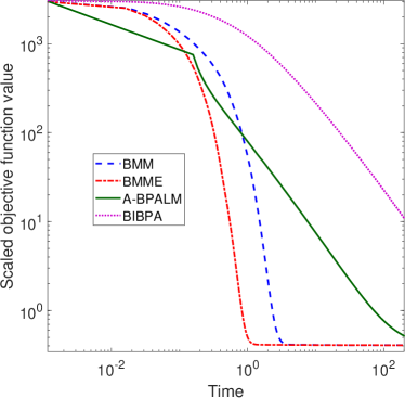
la1	la2

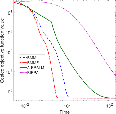
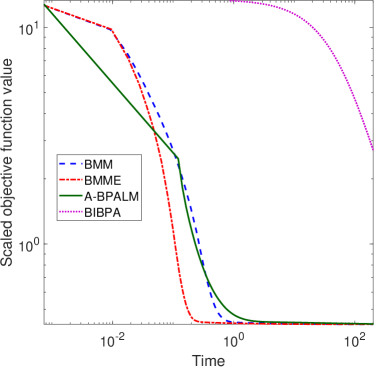
Figure 8: Evolution of scaled objective function values with respect to time on document data sets.

classic	k1bl
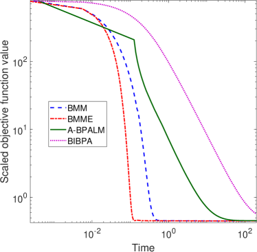
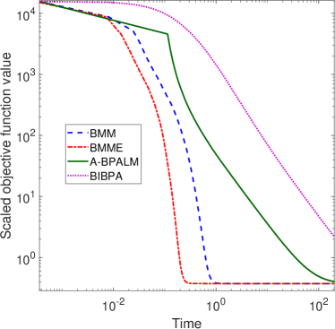
tr11	tr23
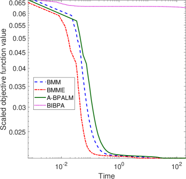
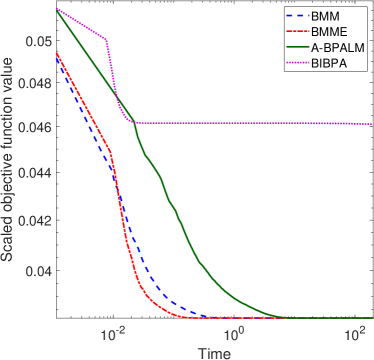
tr41	tr45

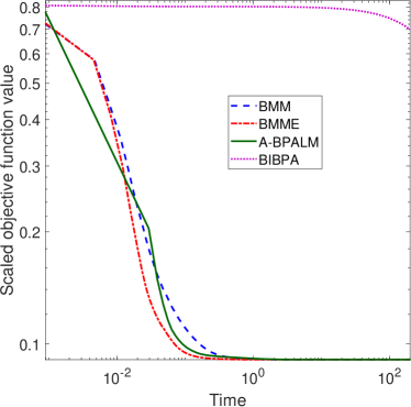
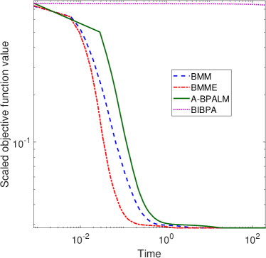
Figure 9: Evolution of scaled objective function values with respect to time on document data sets.

Appendix D Comparison between BMME and CoCaIn on the matrix completion problem

In this section, we consider BMME for solving the CSOP (1) with $m=1$. As $m=1$, we can omit the index $i$. In addition, the relative smooth parameters and the kernel generating distance do not depend on $k$. Therefore, the condition (7) can be rewritten as follows

$$D_{\varphi}(x^{k},\bar{x}^{k})\leq\frac{\delta L}{L+l}D_{\varphi}(x^{k-1},x^{k}),$$

and the update (8) becomes

$$\begin{split}x^{k+1}\in\operatorname*{argmin}_{x\in\mathcal{X}}\biggl{\{}LD_{\varphi}(x,\bar{x}^{k})+\biggl{\langle}\nabla f(\bar{x}^{k}),x\biggr{\rangle}+u(x,x^{k})\biggr{\}}.\end{split}$$

In some applications, the constants $L,l$ might be very large, leading to a slow convergence. Hence, like CoCaIn [25] we incorporate a backtracking line search for $L$ and $l$ into BMME. In particular, BMME with backtracking computes the extrapolation point $\bar{x}^{k}=x^{k}+\beta^{k}(x^{k}-x^{k-1})\in{\rm int\,dom\,}\varphi$, where $\beta^{k}$ satisfies the following condition

$$D_{\varphi}(x^{k},\bar{x}^{k})\leq\frac{\delta L^{k-1}}{L^{k-1}+l^{k}}D_{\varphi}(x^{k-1},x^{k}),$$

where $l^{k}$ is updated via backtracking such that

$$D_{f}(x^{k},\bar{x}^{k})\geq-l^{k}D_{\varphi}(x^{k},\bar{x}^{k}).$$

The update $x^{k+1}$ is computed by solving the following convex nonsmooth sub-problem

$$\min_{x\in\mathcal{X}}\biggl{\{}L^{k}D_{\varphi}(x,\bar{x}^{k})+\biggl{\langle}\nabla f(\bar{x}^{k}),x\biggr{\rangle}+u(x,x^{k})\biggr{\}},$$

where $L^{k}$ is chosen via backtracking such that $L^{k}\geq L^{k-1}$ and

$$D_{f}(x^{k+1},\bar{x}^{k})\leq L^{k}D_{\varphi}(x^{k+1},\bar{x}^{k}).$$

We now conduct an additional experiment on the following matrix completion problem (MCP) to demonstrate the advantages of using proper convex surrogate functions:

(37) $$\min_{U\in\mathbb{R}^{\mathbf{m}\times\mathbf{r}},V\in\mathbb{R}^{\mathbf{r}\times\mathbf{n}}}\biggl{\{}\frac{1}{2}\|\mathcal{P}(A-UV)\|_{F}^{2}+g(U,V)\biggr{\}},$$

where $A\in\mathbb{R}^{\mathbf{m}\times\mathbf{n}}$ is a given data matrix, $\mathcal{P}(Z)_{ij}$ is equal to $Z_{ij}$ if $A_{ij}$ is observed and is equal to $0$ otherwise, and $g$ is a regularization term. Here, we are interested in an exponential regularization $g$ defined by

$$g(U,V)=\lambda\Big{(}\sum_{ij}\big{(}1-\exp(-\theta|U_{ij}|)\big{)}+\sum_{ij}\big{(}1-\exp(-\theta|U_{ij}|)\big{)}\Big{)},$$

where $\lambda$ and $\theta$ are tuning parameters. We consider the problem (37) as the form of (1) with $m=1$, $\mathcal{X}_{1}=\mathcal{X}=\mathbb{R}^{\mathbf{m}\times\mathbf{r}}\times\mathbb{R}^{\mathbf{r}\times\mathbf{n}}$, $f(U,V)=\frac{1}{2}\|\mathcal{P}(A-UV)\|_{F}^{2}$, and $g_{1}(U,V)=g(U,V)$. We now investigate BMME for solving the problem (37) by choosing a kernel generating distance $\varphi$ given by

$$\varphi(U,V)=c_{1}\biggl{(}\frac{\|U\|^{2}_{F}+\|V\|^{2}_{F}}{2}\biggr{)}^{2}+c_{2}\frac{\|U\|^{2}_{F}+\|V\|^{2}_{F}}{2},$$

where $c_{1}=3$ and $c_{2}=\|\mathcal{P}(A)\|_{F}$. In [24], the authors showed that $f$ is $(L,l)$-relative smooth to $\varphi$ for all $L,l\geq 1$. BMME iteratively chooses a convex surrogate function $u$ of $g$ as follows:

$$u(U,V,U^{k},V^{k})=g(U^{k},V^{k})+\langle W^{U^{k}},|U|\rangle+\langle W^{V^{k}},|V|\rangle,$$

where $W^{U^{k}}_{ij}=\lambda\theta\exp(-\theta|U_{ij}^{k}|)$. BMME with backtracking updates $(U^{k+1},V^{k+1})$ by solving the following convex nonsmooth sub-problem

(38) $$\min_{U,V}\biggl{\{}u(U,V,U^{k},V^{k})+\langle P^{k},U\rangle+\langle Q^{k},V\rangle+L^{k}\varphi(U,V)\biggr{\}},$$

where $P^{k}=\nabla_{U}f(\bar{U}^{k},\bar{V}^{k})-L^{k}\nabla_{U}\varphi(\bar{U}^{k},\bar{V}^{k})$, $Q^{k}=\nabla_{V}f(\bar{U}^{k},\bar{V}^{k})-L^{k}\nabla_{V}\varphi(\bar{U}^{k},\bar{V}^{k})$, and $L^{k}$ is chosen via a backtracking line search. The solution to the problem (38) is defined by $U^{k+1}=-\tau^{*}\mathcal{S}(P^{k},W^{U^{k}})/L^{k}$ and $V^{k+1}=-\tau^{*}\mathcal{S}(Q^{k},W^{V^{k}})/L^{k}$, where $\mathcal{S}(A,B)_{ij}=[|A_{ij}|-B_{ij}]_{+}\text{sign}(A_{ij})$, and $\tau^{*}$ is the unique positive real root of

$$c_{1}\biggl{(}\|\mathcal{S}(P^{k},W^{U^{k}})/L^{k}\|^{2}_{F}+\|\mathcal{S}(Q^{k},W^{V^{k}})/L^{k}\|^{2}_{F}\biggr{)}\tau^{3}+c_{2}\tau-1=0.$$

Since CoCaIn [25] does not use the MM step and requires the weakly convexity of $g$, it is different from BMME for updating $(U^{k+1},V^{k+1})$ and initializing $L^{0}$. In particular, CoCaIn iteratively solves the following nonconvex sub-problem

$$\min_{U,V}\biggl{\{}g(U,V)+\langle P^{k},U\rangle+\langle Q^{k},V\rangle+L^{k}\varphi(U,V)\biggr{\}},$$

which does not have closed-form solutions. We therefore employ an MM scheme to solve this sub-problem. For initializing the step-size, CoCaIn requires $L^{0}>\frac{\lambda\theta^{2}}{(1-\delta-\epsilon)c_{2}}$ that might be quite large, where $\epsilon\in(0,1)$ such that $\delta+\epsilon<1$. Unlike CoCaIn, our BMME with backtracking can use any $L^{0}$. The flexibility of the initialization $L^{0}$ may lead to a faster convergence.

In the experiment, we set $\lambda=0.1$, $\theta=5$, $\delta=0.99$, and $l^{0}=0.001$. We initialize $L^{0}=1.0001\frac{\lambda\theta^{2}}{(1-\delta-\epsilon)c_{2}}$ with $\epsilon=0.009$ for CoCaIn while we choose $L^{0}=0.01$ for BMME with backtracking. We carry out the experiment on MovieLens 1M that contains $999,714$ ratings of $6,040$ different users. We choose $\mathbf{r}=5$ and randomly use 70% of the observed ratings for training and the rest for testing. The process is repeated twenty times. We run each algorithm 20 seconds. We are interested in the root mean squared error on the test set: $RMSE=\sqrt{\|\mathcal{P}_{T}(A-UV)\|^{2}/N_{T}}$, where $\mathcal{P}_{T}(Z)_{ij}=Z_{ij}$ if $A_{ij}$ belongs to the test set and $0$ otherwise, $N_{T}$ is the number of ratings in the test set. We plotted the curves of the average value of RMSE and the objective function value versus training time in Figure 10.

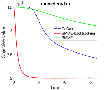
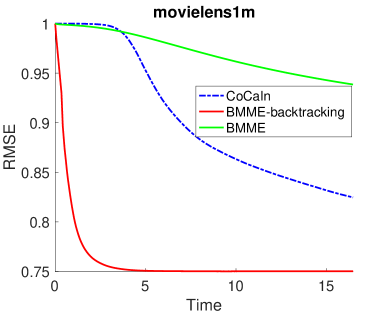
Figure 10: BMME and CoCaIn applied on the MCP (37). Evolution of the average value of the RMSE on the test set and the objective function value with respect to time.

We observe that BMME with backtracking converges much faster than CoCaIn and BMME without backtracking (BMME). This illustrates the usefulness of properly choosing the convex surrogate function and the backtracking line search for the relative smooth constants.

References

- [1] M. Aharon, M. Elad, A. Bruckstein, et al., K-svd: An algorithm for designing overcomplete dictionaries for sparse representation, IEEE Transactions on Signal Processing, 54 (2006), p. 4311.
- [2] M. Ahookhosh, L. T. K. Hien, N. Gillis, and P. Patrinos, A block inertial Bregman proximal algorithm for nonsmooth nonconvex problems with application to symmetric nonnegative matrix tri-factorization, Journal of Optimization Theory and Applications, (2021).
- [3] M. Ahookhosh, L. T. K. Hien, N. Gillis, and P. Patrinos, Multi-block Bregman proximal alternating linearized minimization and its application to sparse orthogonal nonnegative matrix factorization, Computational Optimization and Application, 79 (2021), p. 681–715.
- [4] M. Ahookhosh, A. Themelis, and P. Patrinos, Bregman forward-backward splitting for nonconvex composite optimization: superlinear convergence to nonisolated critical points, SIAM Journal on Optimization, 31 (2021), pp. 653–685.
- [5] U. Araújo, B. Saldanha, R. Galvão, T. Yoneyama, H. Chame, and V. Visani, The successive projections algorithm for variable selection in spectroscopic multicomponent analysis, Chemometrics and Intelligent Laboratory Systems, 57 (2001), pp. 65–73.
- [6] H. Attouch and J. Bolte, On the convergence of the proximal algorithm for nonsmooth functions involving analytic features, Mathematical Programming, 116 (2009), pp. 5–16, https://doi.org/10.1007/s10107-007-0133-5.
- [7] H. Attouch, J. Bolte, P. Redont, and A. Soubeyran, Proximal alternating minimization and projection methods for nonconvex problems: An approach based on the Kurdyka-Łojasiewicz inequality, Mathematics of Operations Research, 35 (2010), pp. 438–457, https://doi.org/10.1287/moor.1100.0449.
- [8] H. Attouch, J. Bolte, and B. F. Svaiter, Convergence of descent methods for semi-algebraic and tame problems: proximal algorithms, forward–backward splitting, and regularized gauss–seidel methods, Mathematical Programming, 137 (2013), pp. 91–129.
- [9] H. H. Bauschke, J. Bolte, and M. Teboulle, A descent lemma beyond Lipschitz gradient continuity: First-order methods revisited and applications, Mathematics of Operations Research, 42 (2017), pp. 330–348, https://doi.org/10.1287/moor.2016.0817.
- [10] A. Beck and L. Tetruashvili, On the convergence of block coordinate descent type methods, SIAM Journal on Optimization, 23 (2013), pp. 2037–2060.
- [11] T. Blumensath and M. E. Davies, Iterative hard thresholding for compressed sensing, Applied and Computational Harmonic Analysis, 27 (2009), pp. 265 – 274, https://doi.org/10.1016/j.acha.2009.04.002.
- [12] J. Bochnak, M. Coste, and M.-F. Roy, Real Algebraic Geometry, Springer, 1998.
- [13] J. Bolte, S. Sabach, and M. Teboulle, Proximal alternating linearized minimization for nonconvex and nonsmooth problems, Mathematical Programming, 146 (2014), pp. 459–494.
- [14] J. Bolte, S. Sabach, M. Teboulle, and Y. Vaisbourd, First order methods beyond convexity and Lipschitz gradient continuity with applications to quadratic inverse problems, SIAM Journal on Optimization, 28 (2018), pp. 2131–2151, https://doi.org/10.1137/17M1138558.
- [15] N. Gillis, Nonnegative Matrix Factorization, SIAM, Philadelphia, 2020.
- [16] N. Gillis, D. Kuang, and H. Park, Hierarchical clustering of hyperspectral images using rank-two nonnegative matrix factorization, IEEE Transactions on Geoscience and Remote Sensing, 53 (2015), pp. 2066–2078.
- [17] N. Gillis and S. A. Vavasis, Fast and robust recursive algorithms for separable nonnegative matrix factorization, IEEE Transactions on Pattern Analysis and Machine Intelligence, 36 (2013), pp. 698–714.
- [18] L. T. K. Hien and N. Gillis, Algorithms for nonnegative matrix factorization with the Kullback-Leibler divergence, Journal of Scientific Computing, (2021), https://doi.org/10.1007/s10915-021-01504-0.
- [19] L. T. K. Hien, N. Gillis, and P. Patrinos, Inertial block proximal method for non-convex non-smooth optimization, in Thirty-seventh International Conference on Machine Learning (ICML), 2020.
- [20] L. T. K. Hien, D. N. Phan, and N. Gillis, Inertial block majorization minimization framework for nonconvex nonsmooth optimization. arXiv:2010.12133, 2020.
- [21] K. Kurdyka, On gradients of functions definable in o-minimal structures, Annales de l’Institut Fourier, 48 (1998), pp. 769–783, https://doi.org/10.5802/aif.1638.
- [22] H. Lu, R. M. Freund, and Y. Nesterov, Relatively smooth convex optimization by first-order methods, and applications, SIAM Journal on Optimization, 28 (2018), pp. 333–354.
- [23] J. Mairal, Optimization with first-order surrogate functions, in Proceedings of the 30th International Conference on International Conference on Machine Learning - Volume 28, ICML’13, JMLR.org, 2013, pp. 783–791.
- [24] M. C. Mukkamala and P. Ochs, Beyond alternating updates for matrix factorization with inertial Bregman proximal gradient algorithms, in Advances in Neural Information Processing Systems 32: Annual Conference on Neural Information Processing Systems 2019, NeurIPS 2019, December 8-14, 2019, Vancouver, BC, Canada, H. M. Wallach, H. Larochelle, A. Beygelzimer, F. d’Alché-Buc, E. B. Fox, and R. Garnett, eds., 2019, pp. 4268–4278.
- [25] M. C. Mukkamala, P. Ochs, T. Pock, and S. Sabach, Convex-concave backtracking for inertial Bregman proximal gradient algorithms in nonconvex optimization, SIAM Journal on Mathematics of Data Science, 2 (2020), pp. 658–682, https://doi.org/10.1137/19M1298007.
- [26] B. Natarajan, Sparse approximate solutions to linear systems, SIAM Journal on Computing, 24 (1995), pp. 227–234, https://doi.org/10.1137/S0097539792240406.
- [27] Y. Nesterov, A method of solving a convex programming problem with convergence rate O, Soviet Mathematics Doklady, 27 (1983).
- [28] Y. Nesterov, Lectures on Convex Optimization, Springer Publishing Company, Incorporated, 2nd ed., 2018.
- [29] P. Ochs, Unifying abstract inexact convergence theorems and block coordinate variable metric ipiano, SIAM Journal on Optimization, 29 (2019), pp. 541–570, https://doi.org/10.1137/17M1124085.
- [30] T. Pock and S. Sabach, Inertial proximal alternating linearized minimization (iPALM) for nonconvex and nonsmooth problems, SIAM Journal on Imaging Sciences, 9 (2016), pp. 1756–1787, https://doi.org/10.1137/16M1064064.
- [31] F. Pompili, N. Gillis, P.-A. Absil, and F. Glineur, Two algorithms for orthogonal nonnegative matrix factorization with application to clustering, Neurocomputing, 141 (2014), pp. 15–25.
- [32] M. Razaviyayn, M. Hong, and Z. Luo, A unified convergence analysis of block successive minimization methods for nonsmooth optimization, SIAM Journal on Optimization, 23 (2013), pp. 1126–1153, https://doi.org/10.1137/120891009.
- [33] M. Teboulle and Y. Vaisbourd, Novel proximal gradient methods for nonnegative matrix factorization with sparsity constraints, SIAM Journal on Imaging Sciences, 13 (2020), pp. 381–421, https://doi.org/10.1137/19M1271750.
- [34] P. Tseng and S. Yun, A coordinate gradient descent method for nonsmooth separable minimization, Mathematical Programming, 117 (2009), pp. 387–423.
- [35] Y. Xu and W. Yin, A block coordinate descent method for regularized multiconvex optimization with applications to nonnegative tensor factorization and completion, SIAM Journal on Imaging Sciences, 6 (2013), pp. 1758–1789, https://doi.org/10.1137/120887795, https://doi.org/10.1137/120887795.
- [36] Y. Xu and W. Yin, A fast patch-dictionary method for whole image recovery, Inverse Problems & Imaging, 10 (2016), p. 563, https://doi.org/10.3934/ipi.2016012.
- [37] Y. Xu and W. Yin, A globally convergent algorithm for nonconvex optimization based on block coordinate update, Journal of Scientific Computing, 72 (2017), pp. 700–734.
- [38] S. Zhong and J. Ghosh, Generative model-based document clustering: a comparative study, Knowledge and Information Systems, 8 (2005), pp. 374–384.