Continual Learning in the Teacher-Student Setup: Impact of Task Similarity

Abstract

Continual learning—the ability to learn many tasks in sequence—is critical for artificial learning systems. Yet standard training methods for deep networks often suffer from catastrophic forgetting, where learning new tasks erases knowledge of earlier tasks. While catastrophic forgetting labels the problem, the theoretical reasons for interference between tasks remain unclear. Here, we attempt to narrow this gap between theory and practice by studying continual learning in the teacher-student setup. We extend previous analytical work on two-layer networks in the teacher-student setup to multiple teachers. Using each teacher to represent a different task, we investigate how the relationship between teachers affects the amount of forgetting and transfer exhibited by the student when the task switches. In line with recent work, we find that when tasks depend on similar features, intermediate task similarity leads to greatest forgetting. However, feature similarity is only one way in which tasks may be related. The teacher-student approach allows us to disentangle task similarity at the level of readouts (hidden-to-output weights) and features (input-to-hidden weights). We find a complex interplay between both types of similarity, initial transfer/forgetting rates, maximum transfer/forgetting, and long-term transfer/forgetting. Together, these results help illuminate the diverse factors contributing to catastrophic forgetting.

1 Introduction

One of the biggest open challenges in machine learning is the ability to effectively perform continual learning: learning tasks sequentially. A significant hurdle in getting systems to do this effectively is that models trained on task A followed by task B will struggle to learn task B without un-learning task A. This is known as catastrophic interference or catastrophic forgetting (McCloskey & Cohen, 1989; Goodfellow et al., 2013), which occurs because weights that contain important information for the first task are overwritten by information relevant to the second. The harmful effects of catastrophic forgetting are not limited to continual learning. They also play a role in multi-task learning, reinforcement learning and standard supervised learning, for example under distribution shift (Arivazhagan et al., 2019; Toneva et al., 2018).

As a result, the phenomenon has received increased interest in recent years. In neuroscience, much work has been done to understand the brain’s ability to consolidate learning from earlier tasks, thereby making it relatively robust to forgetting (Flesch et al., 2018; Cichon & Gan, 2015; Yang et al., 2014). Similarly, a series of works has started a systematic empirical analysis of this phenomenon in deep networks (Parisi et al., 2019; Mirzadeh et al., 2020; Neyshabur et al., 2020; Nguyen et al., 2019; Ruder & Plank, 2017). These works consistently observed a counter-intuitive role of the similarity between tasks A and B, with intermediate task similarity leading to worst forgetting (Ramasesh et al., 2020; Doan et al., 2020; Nguyen et al., 2019).

The purpose of this work is to tackle continual learning from the complementary perspective of high-dimensional teacher-student models (Gardner & Derrida, 1989; Seung et al., 1992; Biehl & Schwarze, 1993; Zdeborová & Krzakala, 2016). These models are a popular framework for studying machine learning problems in a controlled setting, and have recently seen a surge of interest in attempts to understand generalisation in deep neural networks.

Figure 1: Continual learning in the teacher-student setup (a) Illustration of the vanilla teacher-student setup, in which a “student” network is trained on i.i.d. inputs with labels from a “teacher” network. (b) We model continual learning by training a two-layer student (Eqn. 1), on a succession of two teachers, representing distinct tasks $A$ and $B$. (c) Typical generalisation errors of the student ( Eq. 2) w.r.t. both teachers during vs. training step $s$. The solid lines show theoretical predictions derived in subsection 2.1; the crosses are obtained through a single numerical simulation of a networks with input dimension $N=10^{4}$. We also label the key quantities of interest in this study: forgetting, $\mathcal{F}_{t}$ ( Eq. 3), and transfer, $\mathcal{T}_{t}$, ( Eq. 4). Parameters: $M=2$, $K=1$, $V=1$.

Main contributions

• We analyse continual learning in two-layer neural networks by deriving a closed set of equations which predict the test error of the network trained on a succession of tasks using one-pass (or online) SGD, extending classical work on standard supervised learning by Saad & Solla (1995a); Riegler & Biehl (1995).

• Using these equations, we show that intermediate task similarity leads to greatest forgetting in our model.

• We disentangle task similarity on the level of features (input-to-hidden weights) and readouts (input-to-hidden weights) and describe the effect of both types of similarity on forgetting and transfer in infinitely wide networks. We find that feature and readout similarity contribute in complex and sometimes non-symmetric ways to a range of forgetting and transfer metrics.

We summarise our approach in Fig. 1. In the classical teacher-student setup (illustrated in  Fig. 1a), a “student” neural network is trained on synthetic data where inputs $\mathbf{x}\in\mathbb{R}^{D}$ are drawn element-wise i.i.d. from the normal distribution and labels are generated by a “teacher” network (Gardner & Derrida, 1989). To model continual learning, here we consider a setup with two teachers (denoted by $\dagger$ and ${\ddagger}$), which correspond to two tasks to be learned in succession. Let $\phi(\mathbf{x};\mathbf{W},\mathbf{v})$ denote the output of a two-layer network with $L$ hidden neurons, first and second layer weights $\mathbf{W}\in\mathbb{R}^{L\times D}$ and $\mathbf{v}\in\mathbb{R}^{L}$, and activation $g$ after the hidden layer, i.e.

$$\phi(\mathbf{x};\mathbf{W},\mathbf{v})=\sum_{l=1}^{L}{\mathbf{v}}_{l}g\left(\frac{{\mathbf{W}}_{l}\mathbf{x}}{\sqrt{D}}\right).$$ (1)

We generally use $K$ ($M$) for the number of hidden neurons of the student (teacher). In the first phase of training (left side of Fig. 1b), labels are generated by the first teacher via $y^{\dagger}=\phi(\mathbf{x};\mathbf{W}^{\dagger},\mathbf{v}^{\dagger})$, and student outputs are given by $\hat{y}^{\dagger}=\phi(\mathbf{x};\mathbf{W},\mathbf{h}^{\dagger})$. Training proceeds using Stochastic Gradient Descent (SGD) on the squared error of $y^{\dagger}$, $\hat{y}^{\dagger}$ in the online regime, where at each step of SGD we draw a new sample $(x,y)$ to evaluate the gradients, until the task switch. We follow a standard multi-headed approach to continual learning (Zenke et al., 2017; Farquhar & Gal, 2018), in which the student keeps its first-layer weights for the new task, but adds a set of head weights. Thus in the second phase of training, the error is computed over $y^{\ddagger}$, $\hat{y}^{\ddagger}$. Retaining both heads allows us to continually monitor the performance of the student on both tasks after switch, and in theory permits the student to represent both teachers perfectly if given sufficient hidden units.

The generalisation error of the student on the two tasks can be defined as

$$\epsilon^{*}(\mathbf{W},\mathbf{h}^{*},\mathbf{W}^{*},\mathbf{v}^{*})\equiv\\ \frac{1}{2}\left\langle\right.[\phi(\mathbf{x};\mathbf{W}^{*},\mathbf{v}^{*})\left.-\phi(\mathbf{x};\mathbf{W},\mathbf{h}^{*})]^{2}\right\rangle,$$ (2)

where $*$ denotes either task $\dagger$ or ${\ddagger}$, and the average $\langle\cdot\rangle$ is taken over the input distribution $\mathbf{x}$ for a given set of teacher and student weights. Note in the online SGD setting, there is no distinction between train and test error. We emphasise that the student has the same set of first-layer weights ($\mathbf{W}$) for both tasks, but different head weights $\mathbf{h}^{\dagger}$, $\mathbf{h}^{\ddagger}$.

Our main theoretical contribution is a set of dynamical equations that predict the evolution of the test error Eq. 2 during the course of training in the limit of large input dimension $D\to\infty$ with $K,M\sim O(1)$, see Sec. 2. We plot the theoretical prediction in Fig. 1c together with a single simulation (crosses); even at moderate input size $D=10^{4}$, the agreement is good. We observe that the student error on the first task (green) decreases in the first period of training. After switching tasks at $\tilde{s}=5\cdot 10^{5}$, the error of the student on the second task (yellow) decreases, but the error on the first task increases. We define forgetting and transfer at time $\tilde{s}+t$ as

$$\text{Forgetting: }\mathcal{F}_{t} \equiv\epsilon^{\dagger}|_{\tilde{s}+t}-\epsilon^{\dagger}|_{\tilde{s}},$$ (3)

$$\text{Transfer: }\mathcal{T}_{t} \equiv\epsilon^{\ddagger}|_{\tilde{s}}-\epsilon^{\ddagger}|_{\tilde{s}+t},$$ (4)

see Fig. 1c. An increase in error for the first task after the switch corresponds to positive forgetting, while a reduction in error for the second task corresponds to positive transfer. An alternative definition of transfer would compare the performance of the continual learner on task $B$ to the performance of a student that was trained directly on that task. However, this definition introduces additional hyper-parameters which need to be accounted for, such as the distribution of weights at initialisation and at the switching time. Since our focus in this manuscript is on catastrophic forgetting, we focus on the simpler definition of transfer in (4), and leave an exploration of other transfer measures to future work.

A fundamental question in continual learning is the relationship between forgetting/transfer and the task similarity. While one might expect forgetting to decrease with increasing task similarity, Ramasesh et al. (2020)—through a series of careful experiments on the CIFAR10 and CIFAR100 datasets—observed that intermediate task similarity leads to greatest forgetting. We were able to reproduce their results for the two-layer neural networks (1), see App. A.The primary objective of this work is now to use our multi-teacher-student setup, which gives us full control over teacher similarity, to analyse dependence of forgetting and transfer on task similarity theoretically.

1.1 Further Related Work

The teacher-student framework has a long history in studying the dynamics of learning in neural network models (Gardner & Derrida, 1989; Seung et al., 1992; Watkin et al., 1993; Engel & Van den Broeck, 2001; Zdeborová & Krzakala, 2016) and has recently experienced a surge of activity in the machine learning community (Zimmer et al., 2014; Zhong et al., 2017; Tian, 2017; Du et al., 2018; Soltanolkotabi et al., 2018; Aubin et al., 2018; Saxe et al., 2018; Baity-Jesi et al., 2018; Goldt et al., 2019; Ghorbani et al., 2019; Yoshida & Okada, 2019; Ndirango & Lee, 2019; Gabrié, 2020; Bahri et al., 2020; Zdeborová, 2020; Advani et al., 2020). While this article went to press, a preprint by Asanuma et al. (2021) appeared which analyses continual learning in a teacher-student setup for linear regression.

The teacher-student approach has recently been used to study transfer learning, both in linear networks (Lampinen & Ganguli, 2018) and in non-linear perceptron models (Dhifallah & Lu, 2021), which correspond to the $K=M=1$ case of our setup. While the transfer of knowledge from one task to the next is an important aspect in continual learning, the latter is crucially also interested in the retention–or forgetting–of knowledge about the first task. This can be most clearly seen in the fact that in transfer learning, there is only one set of student head weights. Indeed, we will find an interesting interplay between transfer and forgetting in our models of continual learning.

Continual learning in the NTK regime    Doan et al. (2020) analysed the impact of task similarity, and also found increasing task similarity leads to more forgetting. The key difference to our work is that their study focuses on the neural tangent kernel (NTK) (Jacot et al., 2018) or “lazy” regime (Chizat et al., 2019) of two-layer networks, where the first layer of weights stays approximately constant throughout training. Bennani & Sugiyama (2020) gave guarantees on the error achieved with orthogonal gradient descent in the same regime. Here, we focus on the regime where the weights of the network move significantly and are thus able to learn features, which will be key to our analysis in Sec. 2 and to our disentangling of feature vs. readout similarity in Sec. 3.

The dynamics of two-layer neural networks trained using online SGD in the classic teacher-student setup of Fig. 1a was first studied in a series of classic papers by Biehl & Schwarze (1995) and Saad & Solla (1995a) who derived a set of closed ODEs that track the test error of the student (see also Saad & Solla (1995b); Biehl et al. (1996); Saad (2009) for further results and Goldt et al. (2019) for a recent proof of these equations). Here, we extend this type of analysis to the continual learning model of Fig. 1b. The aforementioned works all consider the limit of large input dimension $D\to\infty$, while the number of neurons is of order 1. The complementary “mean-field” limit of finite input dimension and an infinite number of hidden neurons was analysed (Mei et al., 2018; Chizat & Bach, 2018; Sirignano & Spiliopoulos, 2020; Rotskoff & Vanden-Eijnden, 2018). We will turn to this limit to disentangle the impact of feature and readout similarity in Sec. 3.

Many methods for combating catastrophic interference have been proposed, often taking the form of regularisation, architecture expansion, and/or replay (Parisi et al., 2019; Farquhar & Gal, 2018). Regularisation-based methods constrain weights to retain information about earlier tasks (Zenke et al., 2017; Li & Hoiem, 2017; Kirkpatrick et al., 2017); architectural methods add capacity to the network for each new task (Rusu et al., 2016); and replay methods store data from earlier tasks to interleave when learning new tasks (McClelland et al., 1995; Shin et al., 2017).

2 Continual learning in the large input limit

We begin by studying the impact of task similarity on the dynamics and the performance of learning in the limit of large input dimension $D~{}\to~{}\infty$, while the number of neurons $K,M\sim O(1)$.

Training

We train the student using online stochastic gradient descent on the $L_{2}$ loss. Each new input $\mathbf{x}$ is fed to the teacher to compute the target output via $y^{*}=\phi(\mathbf{x};\mathbf{W}^{*},\mathbf{v}^{*})$, while the student prediction is given by $\hat{y}^{\dagger}=\phi(\mathbf{x};\mathbf{W},\mathbf{h}^{*})$. The student’s weights in both layers are updated through gradient descent on $\frac{1}{2}(\hat{y}^{*}-y^{*})^{2}.$ The SGD weight updates are given by:

$$\mathbf{w}_{k}^{\mu+1} =\mathbf{w}_{k}^{\mu}-\frac{\alpha_{\mathbf{W}}}{\sqrt{D}}v_{k}^{*\mu}g^{\prime}(\lambda_{k}^{\mu})\Delta^{*\mu}\mathbf{x}^{\mu}$$ (5a)

$$h_{k}^{*\mu+1} =h_{k}^{*\mu}-\frac{\alpha_{\mathbf{h}}}{D}g(\lambda_{k}^{\mu})\Delta^{*\mu},$$ (5b)

where $\alpha_{\mathbf{W}}$ is the learning rate for the feature weights, $\alpha_{\mathbf{h}}$ is the learning rate for the head weights, and

$$\Delta^{\dagger\mu} \equiv\sum_{k}h_{k}^{\dagger\mu}g(\lambda_{k}^{\mu})-\sum_{m}v_{m}^{\dagger}g(\rho_{m}^{\mu});$$ (6)

$$\Delta^{{\ddagger}\mu} \equiv\sum_{k}h_{k}^{{\ddagger}\mu}g(\lambda_{k}^{\mu})-\sum_{p}v_{p}^{\ddagger}g(\eta_{p}^{\mu}).$$ (7)

We have also introduced the local fields

$$\rho_{m}\equiv\frac{\mathbf{w}_{m}\mathbf{x}}{\sqrt{D}},\qquad\eta_{p}\equiv\frac{\mathbf{w}_{p}\mathbf{x}}{\sqrt{D}},\qquad\lambda_{k}\equiv\frac{\mathbf{w}_{k}\mathbf{x}}{\sqrt{D}}$$ (8)

of the $m^{\text{th}}$ teacher $\dagger$ unit, $n^{\text{th}}$ teacher ${\ddagger}$ unit, and $k^{\text{th}}$ student unit, respectively. In general, indices $i,j,k,l$ are used for hidden units of the student; $m,n$ for hidden units of $\dagger$; and $p,q$ for hidden units of ${\ddagger}$. Initial weights are taken i.i.d. from the normal distribution with standard deviation $\sigma_{0}$. The different scaling of the learning rates for first and second-layer weights guarantees the existence of a well-defined limit of the SGD dynamics as $D\to\infty$. We make the crucial assumption that at each step of the algorithm, we use a previously unseen sample $(\mathbf{x},y^{*})$. This limit of infinite training data is variously known as online learning or one-shot/single-pass SGD. We note that in general the head weights could also be matrices if a teacher has multiple output nodes, but we focus on the case of a single output here to keep notation light.

The “order parameters” of the problem

The key quantity in our analysis is the test error Eq. 2, which (e.g. for $\dagger$) can be written more explicitly as

$$\epsilon^{\dagger}(\mathbf{W},\mathbf{W}^{\dagger},\mathbf{h}^{\dagger},\mathbf{v}^{\dagger})=\\ \frac{1}{2}\left\langle\left[\sum_{k=1}^{K}h_{k}^{\dagger}g(\lambda_{k})-\sum_{m=1}^{M}v_{m}^{\dagger}g(\rho_{m})\right]^{2}\right\rangle.$$ (9)

To evaluate the average, the input $\mathbf{x}$ only appears via products with the student weights $(\lambda_{k})$ and likewise for the teacher; we can hence replace the high-dimensional averages over $\mathbf{x}$ with an average over the $K+M$ “local fields” $\lambda$ and $\rho$. Since we take the inputs element-wise i.i.d. from the standard Gaussian distribution, we have $\langle x_{i}\rangle=0$ and $\langle x_{i}x_{j}\rangle=\delta_{ij}$. It also follows immediately that the local fields are jointly Gaussian, with mean $\langle\lambda_{k}\rangle=\langle\rho_{m}\rangle=0$. The test error can hence be written as a function of only the second moments of the joint distribution of $(\rho,\lambda)$, which we define as

$$q_{kl}\equiv\langle\lambda_{k}\lambda_{l}\rangle,\quad r_{km}\equiv\langle\lambda_{k}\rho_{m}\rangle,\quad t_{mn}\equiv\langle\rho_{m}\rho_{n}\rangle;$$ (10)

and the second-layer weights of the students. In other words, asymptotically

$$\lim_{D\to\infty}\epsilon^{\dagger}(\mathbf{W},\mathbf{W}^{\dagger},\mathbf{h}^{\dagger},\mathbf{v}^{\dagger})=\epsilon^{\dagger}(\mathbf{Q},\mathbf{R},\mathbf{T},\mathbf{h}^{\dagger},\mathbf{v}^{\dagger}).$$ (11)

where $\mathbf{Q}=(q_{kl})$, etc. Note there is an equivalent formulation for ${\ddagger}$ with the $\eta$ local field and relevant second-layer weights. These overlap matrices, or “order parameters” in statistical physics jargon, have a clear physical interpretation, which can be seen when evaluating the averages explicitly. The so-called teacher-student overlap, $r_{km}$ for example:

$$r_{km}\equiv\langle\lambda_{k}\rho_{m}\rangle=\frac{\mathbf{w}_{k}\mathbf{w}_{m}^{\dagger}}{D},$$ (12)

quantifies the overlap or similarity between the weights of the $k^{\text{th}}$ hidden unit of the student and the $m^{\text{th}}$ hidden unit of the teacher. Similarly, $q_{kl}$ gives the self-overlap of the $k$th and $l$th student nodes, and $t_{mn}$ gives the (static) self-overlap of teacher nodes.

Task similarity

The teacher-student setup gives us precise control over the task similarity via the overlap between the first-layer weights of different teachers,

$$v_{mp}\equiv\langle\rho_{m}\eta_{p}\rangle=\frac{1}{D}\mathbf{w}^{\dagger}_{m}\mathbf{w}^{\ddagger}_{p},$$ (13)

which we can tune to observe its effects on the dynamics of continual learning.

2.1 Results

Figure 2: Asymptotic theory matches finite-sized simulations. Plots of progression of generalisation error (a) and order parameters (b-e) for both neural network simulations (crosses) and ODE solutions (solid lines). In this example, the teachers are fully overlapping as evidenced by the identical trajectories of $\mathbf{U}$ and $\mathbf{R}$, the student-teacher^† and student-teacher^‡ overlaps respectively. There is a teacher switch at step 25,000. There is close agreement between the simulation and differential equations (to within the expected $1/\sqrt{N}$ deviation).

Figure 3: The impact of task similarity on continual learning in the large-input limit. a (b): Generalisation error (2) with respect to first (second) teacher (2) during training on two teachers of overlap $V$ computed from the ODEs of Sec. 2. In the first phase of training the generalisation error trivially follows the same trajectory for all teacher-teacher overlaps since the student only knows about one teacher. Post-switch, the generalisation errors follows different paths depending on the relationship between teachers. c (d): Aggregate forgetting (transfer), $\mathcal{F}_{t}$ ($\mathcal{T}_{t}$), vs. teacher-teacher overlap, $V$, at various intervals after task-switch. $V=0$ corresponds to orthogonal teacher weight vectors, $V=1$ corresponds to identical teacher weight vectors. Here we plot with crosses the results achieved with network simulations on top of the lines representing the ODE solutions. Forgetting is strongest for teachers that are intermediately correlated, while the student is relatively robust to forgetting for aligned or orthogonal teachers. Transfer is initially monotonically better for higher overlaps; in the long time limit higher overlap appears to lead to long saddle points that are avoided in lower overlap regimes. Here and throughout, graphs with cold colour tones (greens to blues) refer to the first teacher ($\dagger$), while graphs with warm colour tones (yellows to reds) refer to the second teacher (${\ddagger}$). The deviation of theory and simulation in the top left of (c) is a finite-size effect; the deviation is smaller than $1/\sqrt{N}$. Parameters: $N=10000,M=1,K=2$.

2.1.1 An asymptotically exact theory for the dynamics of continual learning

The test error Eq. 2 can be written in terms of the order parameters Eq. 10, so to compute the test error at all times we need to describe the evolution of $\mathbf{Q}$ etc. during training of the student using SGD Eq. 5. Such equations were derived in the vanilla teacher-student setup by Saad & Solla (1995a); Riegler & Biehl (1995), and here we extend this approach to our continual learning model. We illustrate their derivation for the teacher-student overlap $r_{km}$ Eq. 12. Taking the inner product of Eq. 5a (in the case of $*=\dagger$) with $\mathbf{w}_{n}^{\dagger}$ and substituting the SGD update Eq. 5a yields

$$\mathrm{d}r_{km}^{\mu}\equiv r_{km}^{\mu+1}-r_{km}^{\mu} =\frac{\mathbf{w}_{k}^{\mu+1}\mathbf{w}_{m}^{\dagger}}{D}-\frac{\mathbf{w}_{k}^{\mu}\mathbf{w}_{m}^{\dagger}}{D}$$ (14)

$$=-\frac{\alpha_{\mathbf{W}}}{D}h_{k}^{\dagger\mu}g^{\prime}(\lambda_{k}^{\mu})\Delta^{\dagger\mu}\rho_{m}^{\mu}~{}$$ (15)

In the thermodynamic limit $D\to\infty$, the normalised number of steps $\tau\equiv\mu/D$ becomes a continuous, time-like variable and we can write:

$$\frac{\mathrm{d}r_{kn}}{\mathrm{d}\tau}=-\alpha_{\mathbf{W}}h_{k}^{\dagger}\langle g^{\prime}(\lambda_{k})\Delta^{\dagger}\rho_{n}\rangle.$$ (16)

The remaining averages like $\langle g^{\prime}(\lambda_{k})\lambda_{\ell}g(\rho_{n})\rangle$ are simple three-dimensional integrals over the Gaussian random variables $(\lambda_{k},\lambda_{\ell},\rho_{m})$ and can be evaluated analytically for $g(x)=\mathrm{erf}(x/\sqrt{2})$ and for linear networks with $g(x)=x$. Furthermore, these averages can be expressed only in term of the order parameters, and so the equations close. The ODEs for $\mathbf{Q}$ (Eq. D.9), $\mathbf{U}$ (Eq. D.10), as well as the student head weights, $\mathbf{h}^{\dagger}$, and $\mathbf{h}^{\ddagger}$ (Eq. D.11), are given in App. C.

In Fig. 2, we show test errors and order parameters obtained from numerically solving the ODEs (lines) and from a single simulation (crosses). We find that the agreement between theory and simulations is very good both for the test error and on the level of individual order parameters even at intermediate system size ($D=10^{4}$).

2.1.2 Impact of task similarity

We integrated the ODEs in the simplest possible case to analyse the impact of task similarity. A student with $K=2$ neurons is trained on two teachers with $M=1$ neuron each, all having sigmoidal activation $g(x)=\mathrm{erf}(x/\sqrt{2})$. A subset of the experiments was also carried out on Rectified Linear Unit (ReLU) networks (purely with network simulations) with broadly similar result; details are discussed in App. I. For $M=1$, the task similarity $\mathbf{V}$ (Eq. 13) becomes a scalar quantity that we denote $V$, which is the cosine angle between the teachers’ input-to-hidden weights. We parametrically generate teachers with specified similarities using the procedure described in App. F. The teacher head weights are $\pm{1}$ and the input-hidden weights are normalised. For odd activation functions like the scaled error function, the sign of the input-to-hidden weights can be compensated for by the readout weights so it is sufficient to show results for $V\in[0,1]$. Note that the student has enough capacity to learn both teachers. Fig. 3a shows the generalisation error of the student on the first task, which decays exponentially after an initial period of stationary error. After the switch at $\tilde{s}=1\times 10^{6}$, the learning curves separate depending on the task similarity.

We plot the forgetting Eq. 3 at different times after the switch vs. $V$ in panel c. For teachers with orthogonal first-layer weights ($V=0$), performance on the first task degrades after an initial period of no forgetting. For identical first-layer weights ($V=1$), the initial rate of forgetting is large, but the student recovers and the error on the first task plateaus at a relatively low value. In both cases, forgetting is small compared to teachers with intermediate correlations. Our model thus reproduces the empirical findings on deep networks for image classification from Ramasesh et al. (2020). We hypothesise that while it is intuitive that similar teachers lead to small forgetting, orthogonal teachers can be more easily separated by the student by specialising to the respective teacher units. This separation is made harder by correlations between the weights of the teachers, akin to the problem of source separation in signal processing.

To analyse transfer, we look at the generalisation on the second task ${\ddagger}$ after the switch Fig. 3b. Just after the switch, higher overlap allows faster transfer. All students then reach a second plateau. Only students trained on tasks that are close to orthogonal break away form this second plateau and achieve an exponentially decaying generalisation error, whereas the other students remain stuck. This is a remarkable result, since the same student starting from random initial weights would converge to the second teacher without problem. Indeed, for orthogonal teachers, a student trained to convergence on the first task will have the equivalent of random initial weights for the second task (up to the scaling of the networks), explaining its better performance. Students trained on correlated tasks also converge to the teachers of the first, but this correlated initialisation leads to a loss of performance on the second task. We thus find that task similarity aids short-term transfer but harms long-term transfer in this setting.

3 Disentangling Feature and Read-out Similarity

In the previous sections, the task similarity is measured by the teacher-teacher overlap $V$, which is a metric over the input to hidden weights of the teachers. There is however another notion of task similarity that is relevant for two-layer networks: the read-out similarity, which is a metric over the hidden to output weights. A diagram showing the distinction between these similarities for a toy image task is shown in Fig. 4. Most previous studies (Goodfellow et al., 2013; Ramasesh et al., 2020) have not directly studied this distinction, although Ramasesh et al. (2020) provided evidence that the layers of a deep network that are closer to the input are more responsible to forgetting, pointing to the fact that different layers in a network might have different impact on forgetting. The teacher-student framework allows us to disentangle these different aspects of task similarity in detail.

Figure 4: Distinction between feature similarity and read-out similarity. In a toy image task, a model consists of a set of feature extractors, which produce a feature representation vector from the input. This representation is fed into a subsequent readout function (top). This distinction between feature extractors and readouts leads to two related notions of task similarity: feature similarity (bottom left), which is captured by $\mathbf{V}$ in our framework Eq. 13, and read-out similarity, which we describe using $\tilde{V}$ Eq. 18. Some tasks may require the same features with different read-outs while others require different features but similar read-outs. For concrete examples of these similariity notiions, consider a continual learning task setting involving binary classification on MNIST images where the first task requires distinguishing between odd digits and even digits and the second requires distinguishing between digits less than or equal to 4 and digits greater than 4. Both tasks could be achieved with the same features but different readout functions. On the other hand two tasks where the first consists of counting blue squares and the second counting red circles will require different features but could use the same readout function.

3.1 The Mean-Field Limit of Neural Networks

In the large input-limit networks we were considering previously, the hidden dimensions were small and there was no meaningful way of defining a similarity over the hidden to output weights. For this reason, in this section we consider networks in the mean-field limit of large hidden dimension,

$$\phi(\mathbf{x};\mathbf{W},\mathbf{v})=\frac{1}{M}\sum_{m}^{M}\mathbf{v}_{m}g(\mathbf{W}_{m}\mathbf{x}),$$ (17)

where we let the number of neurons $M\to\infty$ while the input dimension $D$ remains finite. Note the scaling is different here from the definition in Eq. 1. In analogy to Eq. 13, let us define the teacher-teacher read-out similarity as:

$$\tilde{V}=\mathbf{h}^{\dagger}\cdot\mathbf{h}^{\ddagger}.$$ (18)

We can thus control both the feature and readout similarities of the teachers, and measure forgetting and transfer of the student in the $(V,\tilde{V})$ plane. However, the student dynamics cannot be described by the simple set of ODEs from above; instead, the dynamics of the student are captured by the time-evolution of the density $\rho(\bm{\theta})$ of the full set of parameters $\bm{\theta}$ of the network (Mei et al., 2018; Rotskoff & Vanden-Eijnden, 2018; Chizat & Bach, 2018; Sirignano & Spiliopoulos, 2019). This density obeys a partial differential equation,

$$\partial_{t}\rho_{t}(\bm{\theta})=\nabla_{\bm{\theta}}\cdot\left(\rho_{t}(\bm{\theta})\nabla_{\bm{\theta}}\Psi\left(\bm{\theta};\rho_{t}\right)\right)$$ (19)

where $\Psi(\bm{\theta})$ can be thought of as a potential for the dynamics. This PDE is hard to analyse, so for the remainder of the paper, we resort to numerical experiments. Since the output dimension of the regression tasks is 1, we can construct teacher readout weights for a given $\tilde{V}$ with the same procedure as was used for the feature weights in previous sections. For the feature weights in the mean-field regime, we first draw a weight matrix for the first teacher element-wise i.i.d from the normal distribution and orthonormalise it: $\mathbf{W}^{\dagger}=(\mathbf{w}^{\dagger})\in\mathbb{R}^{D\times M}$. For the second teacher, the feature weights are obtained from

$$\mathbf{W}^{\ddagger}=\alpha\mathbf{W}^{\dagger}+(1-\alpha^{2})\mathbf{Z},$$ (20)

where $\mathbf{Z}$ is another $D\times M$ matrix with i.i.d. Gaussian elements, and $0<\alpha<1$ is an interpolation parameter. It can be easily verified that $\alpha$ also can be interpreted as an overlap between the two feature weight matrices, where 0 corresponds to orthogonal features and 1 corresponds to identical features. To make this link clear, we abuse notation slightly and refer to $\alpha$ as $V$ in analogy with previous sections.

3.2 Results

Our results are presented in Fig. 5, where we show (i) the initial rate of forgetting/transfer, (ii) the maximum amount of forgetting/transfer and (iii) the long-time values of forgetting/transfer (the value measured at the end of our training). Details of the procedure used for computing these measures are given in App. L.

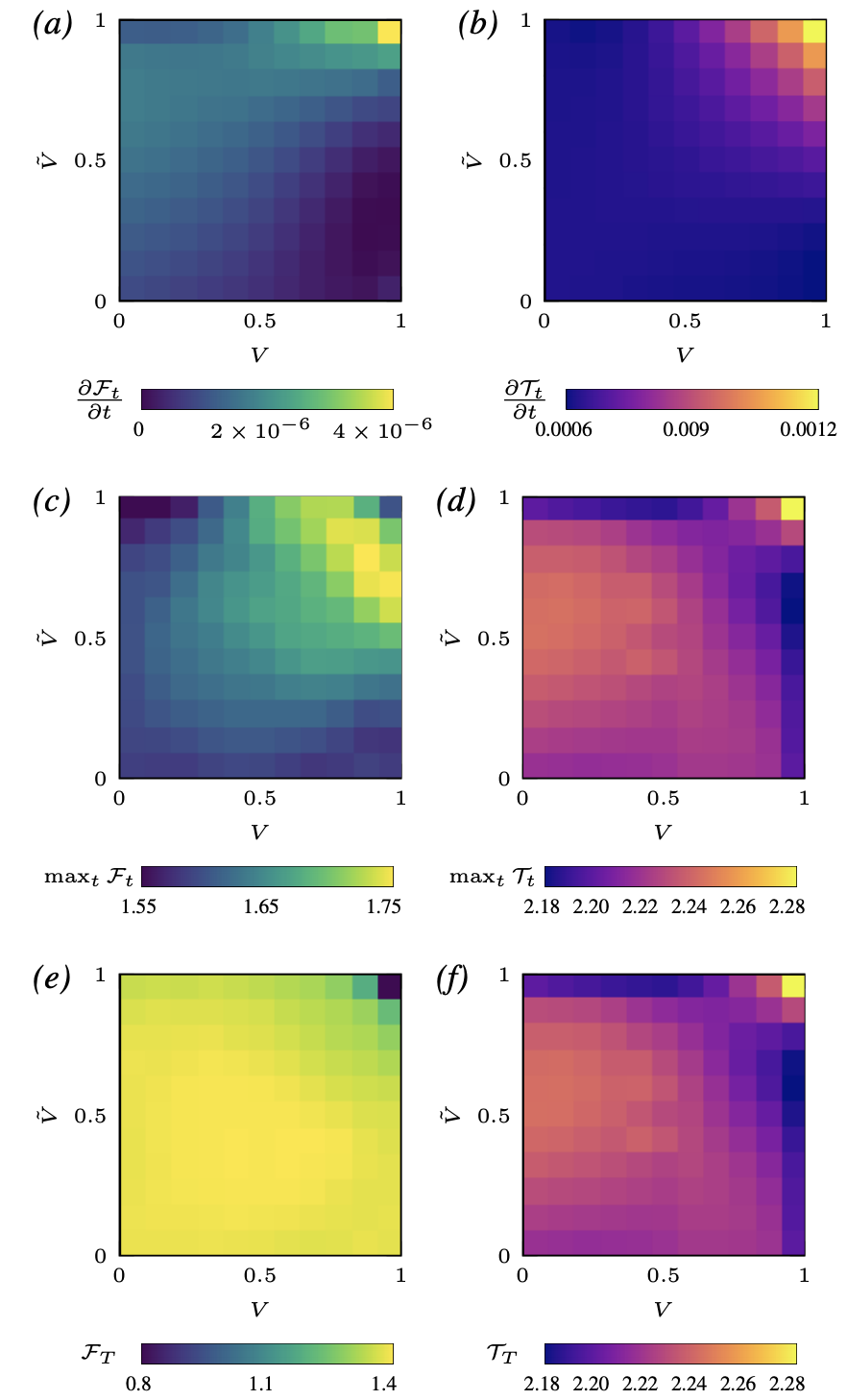
Figure 5: The interplay of transfer and forgetting as a function of feature and readout similarity. (a): Initial rate of forgetting, $\partial\mathcal{F}_{t}/\partial t$; (b): Initial rate of transfer, $\partial\mathcal{T}_{t}/\partial t$; (c): Aggregate (long-time) forgetting, $\mathcal{F}_{T}$; (d): Aggregate (long-time) transfer, $\mathcal{T}_{T}$; (e): Max forgetting reached, $\max_{t}{\mathcal{F}_{t}}$; (f): Max transfer reached, $\max_{t}{\mathcal{T}_{t}}$. All quantities are plotted on a 2D grid of readout similarity $\tilde{V}$ vs. feature similarity $V$ in two-layer networks in the mean-field limit. Parameters: $N=15,M=1000,K=250$.

As a check on our setup, we observe that our results are consistent with the preceding ODE limit simulations, as can be seen from the non-monotonic amount of forgetting for the maximum forgetting metric as a function of input similarity $V$ for full readout similarity ($\tilde{V}=1$, Fig. 5c top row); and the same positive relationship between feature similarity and transfer observed in the early phase of transfer in the ODE limit (Fig. 5d top row). We now turn to describing behaviour in the full space of feature and readout similarities.

3.2.1 Initial Forgetting & Transfer Rate

First, we examine the rate of forgetting and transfer at the moment the tasks are switched (Fig. 5a-b). The transfer rate is approximately constant along each diagonal, such that it is an approximate function of the summed feature and readout similarity $\tilde{V}+V$, indicating that both similarities are roughly interchangeable. By contrast, the forgetting rate shows a differential effect of each similarity type, with high readout similarity causing faster forgetting.

3.2.2 Max & Long-Time Forgetting & Transfer

The results in Fig. 5c-f demonstrate an intricate relationship between each type of task similarity and forgetting/transfer dynamics. We make several observations. First, the maximum and long-time metrics differ substantially for forgetting. For instance, the best scenario for limiting maximum forgetting is orthogonal features and fully aligned readouts ($V=0,\tilde{V}=1$), whereas for long-time forgetting it is complete task overlap ($\tilde{V}=1,V=1$). Intuitively, learning the same task twice might cause transient forgetting, but eventually will converge to the correct features for both tasks. Maximum forgetting is worst in a narrow band of high summed similarity, whereas long-time forgetting is worst at more moderate levels of summed similarity. Intuitively, very similar but subtly different tasks can produce large transient errors which are ultimately corrected at long times. Finally, for a fixed summed similarity $\tilde{V}+V$, forgetting is worst when both similarities are approximately equal. This finding generalises the observation that intermediate task similarity is most harmful to forgetting. For transfer, by contrast, the maximum and long-time metrics are highly correlated and often coincide (the point of maximum transfer is the long-time cutoff in our experiment). Outside of tasks that overlap completely, there is a slight trend for better transfer at moderate readout similarity and low feature similarity.

For a constant feature or readout similarity (that is, isolating any column or row with fixed $V$ or $\tilde{V}$ respectively), we typically observe a non-monotonic relationship between similarity and forgetting that peaks at some intermediate level of similarity. Hence the finding that intermediate amounts of similarity cause greatest forgetting, observed in the ODE limit, holds true at most fixed similarities (see App. M for details).

Finally, we note that transfer depends on readout similarity even for teachers with identical features. Readout similarity has a non-monotonic effect, as can be seen in the column corresponding to full feature similarity ($V=1$). This finding occurs despite the fact that the student network uses a distinct readout head for each task. We surmise that the readout weights bias the solution found by the student for the feature weights during training on the first task. This bias can have the effect of favouring subsequent learning with respect to a second teacher with readout weights that are more similar to those of the first. We show further empirical evidence for this phenomenon in App. N.

4 Conclusion

Overall, our results depict a complex relationship between task similarity, forgetting, and transfer dynamics. The degree of readout and feature similarity, as well as the timing and form of measurements, all matter in determining the outcome even qualitatively. By characterising the continual learning behaviour of simple gradient descent, we hope our experiments and theoretical framework will serve as a useful foundation for future investigations into the effect of proposed solutions for continual learning in the teacher-student setup, ultimately leading to improved algorithms.

Appendix A Reproducing the results of Ramasesh et al. with two-layer neural networks

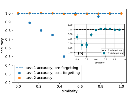
Figure 6: Task similarity in deep vs. shallow networks We plot the accuracy of a two-layer ReLU network with 8 neurons trained on two tasks. The first task is discriminating T-shirts from high-heels on Fashion MNIST (task 1). The second task is a linear interpolation in both inputs and labels between task 1 and long-sleeve shirts vs trainers. In the inset, we reproduce Fig. 5b of Ramasesh et al. (2020) when training various deep networks on two tasks obtained by linearly interpolation of CIFAR10 images. Parameters of our experiment: learning rate 0.01, $D=784$.

We report in Fig. 6 a reproduction of an experiment showing that the two-layer networks trained on FashionMNIST (Xiao et al., 2017) reproduce a key observation of (Ramasesh et al., 2020) made for VGG, ResNet and DenseNet on CIFAR10: intermediate task similarity leads to worst forgetting. To that end, we trained a two-layer ReLU network with 8 neurons to discriminate T-shirts from high-heels on Fashion MNIST (task 1). The second task was a linear interpolation in both inputs and labels between task 1 and long-sleeve shirts vs trainers. We see that at intermediate task similarity, or halfway along the linear interpolation between the two datasets, forgetting of the first task is the worst. This is the same behaviour Ramasesh et al. (2020) found consistently for VGG, ResNet and DenseNet when linearly interpolating CIFAR10 images (we reproduce their Fig. 5b in the inset). Hence the toy model studied here reproduces this behaviour of more realistic setups.

Appendix B Order Parameters

The full set of order parameters for the two-teacher student-teacher networks in the large input limit is given by:

$$\text{\footnotesize Student-Student Overlap, }\mathbf{Q}:q_{kl} \equiv\langle\lambda_{k}\lambda_{l}\rangle=\frac{1}{N}\mathbf{w}_{k}\mathbf{w}_{l};$$ (B.1)

$$\text{\footnotesize Teacher}^{\dagger}\text{\footnotesize-Teacher}^{\dagger}\text{\footnotesize Overlap, }\mathbf{T}:t_{nm} \equiv\langle\rho_{m}\rho_{n}\rangle=\frac{1}{N}\mathbf{w}^{\dagger}_{m}\mathbf{w}^{\dagger}_{n};$$ (B.2)

$$\text{\footnotesize Student-Teacher}^{\dagger}\text{\footnotesize Overlap, }\mathbf{R}:r_{km} \equiv\langle\lambda_{k}\rho_{m}\rangle=\frac{1}{N}\mathbf{w}_{k}\mathbf{w}^{\dagger}_{m};$$ (B.3)

$$\text{\footnotesize Teacher}^{\ddagger}\text{\footnotesize-Teacher}^{\ddagger}\text{\footnotesize Overlap, }\mathbf{S}:s_{pq} \equiv\langle\eta_{p}\eta_{q}\rangle=\frac{1}{N}\mathbf{w}^{\ddagger}_{p}\mathbf{w}^{\ddagger}_{q};$$ (B.4)

$$\text{\footnotesize Student-Teacher}^{\ddagger}\text{\footnotesize Overlap, }\mathbf{U}:u_{kp} \equiv\langle\lambda_{k}\eta_{p}\rangle=\frac{1}{N}\mathbf{w}_{k}\mathbf{w}^{\ddagger}_{p};$$ (B.5)

$$\text{\footnotesize Teacher}^{\dagger}\text{\footnotesize-Teacher}^{\ddagger}\text{\footnotesize Overlap, }\mathbf{V}:v_{mp} \equiv\langle\rho_{m}\eta_{p}\rangle=\frac{1}{N}\mathbf{w}^{\dagger}_{m}\mathbf{w}^{\ddagger}_{p}.$$ (B.6)

Appendix C ODE Derivation

This section presents the derivation of the ODE formulation of the generalisation error for the student-multi-teacher continual learning framework.

C.1 Generalisation Error in terms of Order Parameters

Our aim is to formulate the generalisation error in terms of the macroscopic order parameters. Let us begin by multiplying out Eq. 2,

$$\epsilon_{g}^{\dagger}=\frac{1}{2}\left\langle\left[\sum_{i,k}h_{i}^{\dagger}h_{k}^{\dagger}g(\lambda_{i})g(\lambda_{k})+\sum_{m,n}v_{m}^{\dagger}v_{n}^{\dagger}g(\rho_{m})g(\rho_{n})-2\sum_{i,n}h_{i}^{\dagger}v_{n}^{\dagger}g(\lambda_{i})g(\rho_{n})\right]\right\rangle.$$ (C.1)

and similarly for the second student. These generalisation errors involve averages of local fields, which can be computed as integrals over a joint multivariate Gaussian probability distribution, all of the form

$$\mathcal{P}(\beta,\gamma)=\frac{1}{\sqrt{(2\pi)^{F+H}|\tilde{\mathbf{C}}|}}\exp{\left\{-\frac{1}{2}(\beta,\gamma)^{T}\tilde{\mathbf{C}}^{-1}(\beta,\gamma)\right\}},$$ (C.2)

where $\beta$ and $\gamma$ are local fields with number of units $F$ and $H$ respectively, and $\tilde{\mathbf{C}}$ is a covariance matrix suitably projected down from

$$\mathbf{C}=\begin{pmatrix}\mathbf{Q}&\mathbf{R}&\mathbf{U}\\ \mathbf{R}^{T}&\mathbf{T}&\mathbf{V}\\ \mathbf{U}^{T}&\mathbf{V}^{T}&\mathbf{S}\end{pmatrix}.$$

We define

$$I_{2}(f,h)\equiv\langle g(\beta)g(\gamma)\rangle,$$ (C.3)

where $f,h$ are the indices corresponding to the units of the local fields $\beta$ and $\gamma$. This allows us to write the generalisation errors as

$$\epsilon_{g}^{\dagger} =\frac{1}{2}\sum_{i,k}h^{\dagger}_{i}h^{\dagger}_{k}I_{2}(i,k)+\frac{1}{2}\sum_{n,m}v^{\dagger}_{n}v^{\dagger}_{m}I_{2}(n,m)-\sum_{i,n}h^{\dagger}_{i}v^{\dagger}_{n}I_{2}(i,n)$$ (C.4)

$$\epsilon_{g}^{\ddagger} =\frac{1}{2}\sum_{i,k}h^{\ddagger}_{i}h^{\ddagger}_{k}I_{2}(i,k)+\frac{1}{2}\sum_{p,q}v^{\ddagger}_{p}v^{\ddagger}_{q}I_{2}(p,q)-\sum_{i,p}h^{\ddagger}_{i}v^{\ddagger}_{p}I_{2}(i,p).$$ (C.5)

C.1.1 Sigmoidal Activation

For the scaled error activation function, $g(x)=\text{erf}(x/\sqrt{2})$, there is an analytic expression for the $I_{2}$ integral purely in terms of the order parameters (Saad & Solla, 1995a):

$$I_{2}(i,k)=\frac{1}{\pi}\arcsin{\frac{q_{ik}}{\sqrt{(1+q_{ii})(1+q_{kk})}}}.$$ (C.6)

In turn, we can similarly write the generalisation errors in terms of the order parameters only:

$$\epsilon_{g}^{\dagger}=\frac{1}{\pi}\sum_{i,k}h^{\dagger}_{i}h^{\dagger}_{k}\arcsin{\frac{q_{ik}}{\sqrt{(1+q_{ii})(1+q_{kk})}}}+\frac{1}{\pi}\sum_{n,m}v^{\dagger}_{n}v^{\dagger}_{m}\arcsin{\frac{t_{nm}}{\sqrt{(1+t_{nn})(1+t_{mm})}}}\\ +\frac{2}{\pi}\sum_{i,n}h^{\dagger}_{i}v^{\dagger}_{n}\arcsin{\frac{r_{in}}{\sqrt{(1+q_{ii})(1+t_{nn})}}}$$ (C.7)

$$\epsilon_{g}^{\ddagger}=\frac{1}{\pi}\sum_{i,k}h^{\ddagger}_{i}h^{\ddagger}_{k}\arcsin{\frac{q_{ik}}{\sqrt{(1+q_{ii})(1+q_{kk})}}}+\frac{1}{\pi}\sum_{p,q}v^{\ddagger}_{p}v^{\ddagger}_{q}\arcsin{\frac{s_{pq}}{\sqrt{(1+s_{pp})(1+s_{qq})}}}\\ +\frac{2}{\pi}\sum_{i,p}h^{\ddagger}_{i}v^{\ddagger}_{p}\arcsin{\frac{u_{ip}}{\sqrt{(1+q_{ii})(1+s_{pp})}}}.$$ (C.8)

C.2 Order Parameter Evolution (Training on $\dagger$)

Having arrived at expressions for the generalisation error of both teachers in terms of the order parameters, we want to determine equations of motion for these order parameters from the weight update equations (Eq. 5a & Eq. 5b). Trivially, the order parameters associated with the two teachers, $\mathbf{T}$ and $\mathbf{S}$ are constant over time, as are the head weights of the teachers, $\mathbf{v}^{\dagger},\mathbf{v}^{\ddagger}$. When training on $\dagger$, the student head weights corresponding to ${\ddagger}$ are also stationary; it remains for us to find equations of motion for $\mathbf{R},\mathbf{Q},\mathbf{U}$ and $\mathbf{h}^{\dagger}$, which we derive below. The equivalent derivations when training on teacher ${\ddagger}$ can be made by using the update in Eq. 5b instead.

C.2.1 ODE for $\mathbf{R}$

Consider the inner product of Eq. 5a (in the case of * = $\dagger$) with $\mathbf{w}_{n}^{\dagger}$:

$$\mathbf{w}_{k}^{\mu+1}\mathbf{w}_{n}^{\dagger}-\mathbf{w}_{k}^{\mu}\mathbf{w}_{n}^{\dagger} =-\frac{\alpha_{\mathbf{W}}}{\sqrt{D}}h_{k}^{\dagger\mu}g^{\prime}(\lambda_{k}^{\mu})\Delta^{\dagger\mu}\mathbf{x}^{\mu}\mathbf{w}_{n}^{\dagger}$$ (C.9)

$$=-\alpha_{\mathbf{W}}h_{k}^{\dagger\mu}g^{\prime}(\lambda_{k}^{\mu})\Delta^{\dagger\mu}\rho_{n}^{\mu}$$ (C.10)

$$r_{kn}^{\mu+1}-r_{kn}^{\mu} =-\frac{\alpha_{\mathbf{W}}}{D}h_{k}^{\dagger\mu}g^{\prime}(\lambda_{k}^{\mu})\Delta^{\dagger\mu}\rho_{n}^{\mu}$$ (C.11)

If we let $\tau\equiv\mu/D$ and take the thermodynamic limit of $D\to\infty$, the time parameter becomes continuous and we can write:

$$\frac{dr_{in}}{d\tau}=-\alpha_{\mathbf{W}}h_{i}^{\dagger}\langle g^{\prime}(\lambda_{i})\Delta^{\dagger}\rho_{n}\rangle,$$ (C.12)

where we have re-indexed $k\to i$.

C.2.2 ODE for $\mathbf{Q}$

Consider squaring Eq. 5a (here we can simply use * to denote training on either teacher).

$$\mathbf{w}_{k}^{\mu+1}\mathbf{w}_{i}^{\mu+1}-\mathbf{w}_{k}^{\mu}\mathbf{w}_{i}^{\mu} =-\frac{\alpha_{\mathbf{W}}}{\sqrt{D}}h_{i}^{*\mu}g^{\prime}(\lambda_{i}^{\mu})\Delta^{*\mu}\mathbf{x}^{\mu}\mathbf{w}_{k}^{\mu}-\frac{\alpha_{\mathbf{W}}}{\sqrt{D}}h_{k}^{*\mu}g^{\prime}(\lambda_{k}^{\mu})\Delta^{*\mu}\mathbf{x}^{\mu}\mathbf{w}_{i}^{\mu}$$

$$\quad\quad+\frac{\alpha_{\mathbf{W}}^{2}}{D}h_{i}^{*\mu}g^{\prime}(\lambda_{i}^{\mu})h_{k}^{*\mu}g^{\prime}(\lambda_{k}^{\mu})(\Delta^{*\mu}\mathbf{x}^{\mu})^{2}$$ (C.13)

$$=-\alpha_{\mathbf{W}}h_{i}^{*\mu}g^{\prime}(\lambda_{i}^{\mu})\Delta^{*\mu}\lambda_{k}^{\mu}-\alpha_{\mathbf{W}}h_{k}^{*\mu}g^{\prime}(\lambda_{k}^{\mu})\Delta^{*\mu}\lambda_{i}^{\mu}$$

$$\quad\quad+\frac{\alpha_{\mathbf{W}}^{2}}{D}h_{i}^{*\mu}g^{\prime}(\lambda_{i}^{\mu})h_{k}^{*\mu}g^{\prime}(\lambda_{k}^{\mu})(\Delta^{*\mu}\mathbf{x}^{\mu})^{2}$$ (C.14)

$$q^{\mu+1}_{ki}-q^{\mu}_{ki} =-\frac{\alpha_{\mathbf{W}}}{D}h_{i}^{*\mu}g^{\prime}(\lambda_{i}^{\mu})\Delta^{*\mu}\lambda_{k}^{\mu}-\frac{\alpha_{\mathbf{W}}}{D}h_{k}^{*\mu}g^{\prime}(\lambda_{k}^{\mu})\Delta^{*\mu}\lambda_{i}^{\mu}$$

$$\quad\quad+\frac{\alpha_{\mathbf{W}}^{2}}{D^{2}}h_{i}^{*\mu}g^{\prime}(\lambda_{i}^{\mu})h_{k}^{*\mu}g^{\prime}(\lambda_{k}^{\mu})(\Delta^{*\mu}\mathbf{x}^{\mu})^{2}.$$ (C.15)

Performing the same reparameterisation of $\mu$ and the same thermodynamic limit, we get:

$$\frac{dq_{ik}}{d\tau}=-\alpha_{\mathbf{W}}h_{i}^{*}\langle g^{\prime}(\lambda_{i})\Delta^{*}\lambda_{k}\rangle-\alpha_{\mathbf{W}}h_{k}^{*}\langle g^{\prime}(\lambda_{k})\Delta^{*}\lambda_{i}\rangle+\alpha_{\mathbf{W}}^{2}h_{i}^{*}h_{k}^{*}\langle g^{\prime}(\lambda_{i})g^{\prime}(\lambda_{k})\Delta^{*2}\rangle.$$ (C.16)

Note: in the limit, $(\mathbf{x}^{\mu})^{2}\to D$ since individual samples are taken from a unit normal. Hence the $1/D$ limit remains the same decay rate for each term.

C.2.3 ODE for $\mathbf{U}$

Consider the inner product of Eq. 5a (in the case of * = $\dagger$) with $\mathbf{w}_{p}^{\ddagger}$:

$$\mathbf{w}_{k}^{\mu+1}\mathbf{w}_{p}^{\ddagger}-\mathbf{w}_{k}^{\mu}\mathbf{w}_{p}^{\ddagger} =-\frac{\alpha_{\mathbf{W}}}{\sqrt{D}}h_{k}^{\dagger\mu}g^{\prime}(\lambda_{k}^{\mu})\Delta^{\dagger\mu}\mathbf{x}^{\mu}\mathbf{w}_{p}^{\ddagger}$$ (C.17)

$$=-\alpha_{\mathbf{W}}h_{k}^{\dagger\mu}g^{\prime}(\lambda_{k}^{\mu})\Delta^{\dagger\mu}\eta_{p}^{\mu}$$ (C.18)

$$u_{kp}^{\mu+1}-u_{kp}^{\mu} =-\frac{\alpha_{\mathbf{W}}}{D}h_{k}^{\dagger\mu}g^{\prime}(\lambda_{k}^{\mu})\Delta^{\dagger\mu}\eta_{p}^{\mu}.$$ (C.19)

If we let $\tau\equiv\mu/D$ and take the thermodynamic limit of $D\to\infty$:

$$\frac{du_{ip}}{d\tau}=-\alpha_{\mathbf{W}}h_{i}^{*}\langle g^{\prime}(\lambda_{i})\Delta^{*}\eta_{p}\rangle.$$ (C.20)

C.2.4 ODE for $\mathbf{h}^{*}$

Here, we simply take the thermodynamic limit of Eq. 5b (for * = $\dagger$):

$$\frac{dh_{i}^{\dagger}}{d\tau}=-\alpha_{h}\langle\Delta^{\dagger}g(\lambda_{i})\rangle$$ (C.21)

Appendix D Explicit Formulation

We can go one step further and write the right hand sides of the ODEs in terms of more concise integrals. Recall that for no noise

$$\Delta^{\dagger\mu}\equiv\sum_{k}h_{k}^{\dagger\mu}g(\lambda_{k}^{\mu})-\sum_{m}v_{m}^{\dagger}g(\rho_{m}^{\mu}).$$ (D.1)

Substituting this term into the ODEs above gives us the expanded versions below:

$$\frac{dr_{in}}{d\tau} =-\alpha_{\mathbf{W}}h_{i}^{\dagger}\left\langle g^{\prime}(\lambda_{i})\left[\sum_{k}h_{k}^{\dagger}g(\lambda_{k})-\sum_{m}v_{m}^{\dagger}g(\rho_{m})\right]\rho_{n}\right\rangle;$$ (D.2)

$$\frac{dq_{ik}}{d\tau} =-\alpha_{\mathbf{W}}h_{i}^{\dagger}\left\langle g^{\prime}(\lambda_{i})\left[\sum_{j}h_{j}^{\dagger}g(\lambda_{j})-\sum_{m}v_{m}^{\dagger}g(\rho_{m})\right]\lambda_{k}\right\rangle$$

$$\quad\quad-\alpha_{\mathbf{W}}h_{k}^{\dagger}\left\langle g^{\prime}(\lambda_{k})\left[\sum_{j}h_{j}^{\dagger}g(\lambda_{j})-\sum_{m}v_{m}^{\dagger}g(\rho_{m})\right]\lambda_{i}\right\rangle$$

$$\quad\quad\quad+\alpha_{\mathbf{W}}^{2}h_{i}^{\dagger}h_{k}^{\dagger}\left\langle g^{\prime}(\lambda_{i})g^{\prime}(\lambda_{k})\left[\sum_{j}h_{j}^{\dagger}g(\lambda_{j})-\sum_{m}v_{m}^{\dagger}g(\rho_{m})\right]^{2}\right\rangle;$$ (D.3)

$$\frac{du_{ip}}{d\tau} =-\alpha_{\mathbf{W}}h_{i}^{\dagger}\left\langle g^{\prime}(\lambda_{i})\left[\sum_{k}h_{k}^{\dagger}g(\lambda_{k})-\sum_{m}v_{m}^{\dagger}g(\rho_{m})\right]\eta_{p}\right\rangle;$$ (D.4)

$$\frac{dh_{i}^{\dagger}}{d\tau} =-\alpha_{\mathbf{h}}\left\langle\left[\sum_{k}h_{k}^{\dagger}g(\lambda_{k})-\sum_{m}v_{m}^{\dagger}g(\rho_{m})\right]g(\lambda_{i})\right\rangle.$$ (D.5)

Similarly to the $I_{2}$ integral defined in Eq. C.3, we further define:

$$I_{3}(d,f,h)=\langle g^{\prime}(\zeta)\beta g(\gamma)\rangle,$$ (D.6)

$$I_{4}(d,e,f,h)=\langle g^{\prime}(\zeta)g^{\prime}(\iota)g(\beta)g(\gamma)\rangle;$$ (D.7)

where $\zeta,\iota$ are local fields of the student with indices $d,e$; and $\beta,\gamma$ can be local fields of either student or teacher with indices $f,h$. Substituting these definitions into the expanded ODE formulations gives:

$$\frac{dr_{in}}{d\tau} =\alpha_{\mathbf{W}}h_{i}^{\dagger}\left[\sum_{m}^{M}v_{m}^{*}I_{3}(i,n,m)-\sum_{k}^{K}h_{k}^{\dagger}I_{3}(i,n,k)\right];$$ (D.8)

$$\frac{dq_{ik}}{d\tau} =\alpha_{\mathbf{W}}h_{i}^{\dagger}\left[\sum_{m}^{M}v^{\dagger}_{m}I_{3}(i,k,m)-\sum_{j}^{K}h^{\dagger}_{j}I_{3}(i,k,j)\right]$$

$$\quad+\alpha_{\mathbf{W}}h_{k}^{\dagger}\left[\sum_{m}^{M}v^{\dagger}_{m}I_{3}(k,i,m)-\sum_{j}^{K}h^{\dagger}_{j}I_{3}(k,i,j)\right]$$

$$\quad\quad+\alpha_{\mathbf{W}}^{2}h_{i}^{\dagger}h_{k}^{\dagger}\left[\sum_{j,l}^{K}h^{\dagger}_{j}h^{\dagger}_{l}I_{4}(i,k,j,l)+\sum_{m,n}^{M}v^{\dagger}_{m}v^{\dagger}_{n}I_{4}(i,k,m,n)\right.$$

$$\quad\quad\quad\quad\quad\quad\left.-2\sum_{j}^{K}\sum_{m}^{M}v^{\dagger}_{m}h^{\dagger}_{j}I_{4}(i,k,j,m)\right];$$ (D.9)

$$\frac{du_{ip}}{d\tau} =\alpha_{\mathbf{W}}h_{i}^{\dagger}\left[\sum_{m}^{M}v^{\dagger}_{m}I_{3}(i,p,m)-\sum_{k}^{K}h^{\dagger}_{k}I_{3}(i,p,k)\right];$$ (D.10)

$$\frac{dh_{i}^{\dagger}}{d\tau} =\alpha_{\mathbf{h}}\left[\sum_{m}^{M}v^{\dagger}_{m}I_{2}(m,i)-\sum_{k}^{K}h^{\dagger}_{k}I_{2}(k,i)\right].$$ (D.11)

This completes the picture for the dynamics of the generalisation error. It can be expressed purely in terms of the head weights and the $I$ integrals. For the case of the scaled error function we can evaluate the $I_{2},I_{3}$, and $I_{4}$ analytically meaning we have an exact formulation of the generalisation error dynamics of the student with respect to both teachers in the thermodynamic limit. Further details on the integrals can be found in App. E. The next chapter introduces the experimental framework that compliments the theoretical formalism presented above.

Appendix E Gaussian Integrals under Scaled Error Function

In the derivations of App. C, we introduce a set of integrals over multivariate Gaussian distributions, labelled $I_{2}$, $I_{3}$ and $I_{4}$. They are defined as:

$$I_{2}(f,h) \equiv\langle g(\beta)g(\gamma)\rangle,$$ (E.1)

$$I_{3}(d,f,h) \equiv\langle g^{\prime}(\zeta)\beta g(\gamma)\rangle,$$ (E.2)

$$I_{4}(d,e,f,h) \equiv\langle g^{\prime}(\zeta)g^{\prime}(\iota)g(\beta)g(\gamma)\rangle;$$ (E.3)

where $\zeta,\iota$ are local fields of the student with indices $d,e$; and $\beta,\gamma$ can be local fields of either student or teacher with indices $f,h$; and $g$ is the activation function.

These integrals do not have closed form solutions for the ReLU activation. For the scaled error function however, they can all be solved analytically. They are given by:

$$I_{2} =\frac{1}{\pi}\arcsin{\frac{c_{12}}{\sqrt{(1+c_{11})(1+c_{22})}}};$$ (E.4)

$$I_{3} =\frac{2c_{23}(1+c_{11})-2c_{12}c_{13}}{\sqrt{\Lambda_{3}}(1+c_{11})};$$ (E.5)

$$I_{4} =\frac{4}{\pi^{2}\sqrt{\Lambda_{4}}}\arcsin{\frac{\Lambda_{0}}{\sqrt{\Lambda_{1}\Lambda_{2}}}};$$ (E.6)

where

$$\Lambda_{0} =\Lambda_{4}c_{34}-c_{23}c_{24}(1+c_{11})-c_{13}c_{14}(1+c_{22})+c_{12}c_{13}c_{24}+c_{12}c_{14}c_{23};$$ (E.7)

$$\Lambda_{1} =\Lambda_{4}(1+c_{33})-c_{23}^{2}(1+c_{11})-c_{13}^{2}(1+c_{22})+2c_{12}c_{13}c_{23};$$ (E.8)

$$\Lambda_{2} =\Lambda_{4}(1+c_{44})-c_{24}^{2}(1+c_{11})-c_{14}^{2}(1+c_{22})+2c_{12}c_{14}c_{24};$$ (E.9)

$$\Lambda_{3} =(1+c_{11})(1+c_{33})-c_{13}^{2};$$ (E.10)

and where $c$ is the relevant projected down covariance matrix.

Appendix F Overlap Generation

In subsubsection 2.1.2, we investigate the effect of task similarity on forgetting. In our framework, the teachers act as tasks. From App. C, we know that the learning dynamics in the student can be fully described by the overlap parameters, which includes the teacher-teacher overlap matrix, $V$. For our investigation we need a method to generate teachers with specific overlaps; specifically— in the normalised teachers Ansatz, and for teachers with a single hidden unit—we perform simulations over the full range of $V$ from 0 to 1. In this configuration we simply need a procedure to generate two $N$-dimensional vectors, $\mathbf{v}_{1}$, $\mathbf{v}_{2}$, with an angle $\theta$ between them such that:

$$\mathbf{v}_{1}\cdot\mathbf{v}_{2}=\theta.$$ (F.1)

Fortunately there is a standard algorithm for this. First we define two vectors

$$\tilde{\mathbf{v}}_{1}=\begin{pmatrix}0\\ 1\end{pmatrix};\quad\tilde{\mathbf{v}}_{2}=\begin{pmatrix}\sin{\theta}\\ \cos{\theta}\end{pmatrix}.$$

Second, we generate an $N\times N$ orthogonal matrix, $R$. There is a standard sicpy implementation for this based on QR decomposition of a random Gaussian matrix.

Finally, multiply the first two columns of $R$ with either vector to generate the rotated vectors:

$$\mathbf{v}_{1}=R[:,1:2]\cdot\tilde{\mathbf{v}}_{1};$$ (F.2)

$$\mathbf{v}_{2}=R[:,1:2]\cdot\tilde{\mathbf{v}}_{2}.$$ (F.3)

Appendix G Experiment Details

In this section we provide details of experimental procedures used to obtain the graphs and figures presented in this work.

In the ODE limit investigation, the following parameters were used:

• Input dimension = 10,000;

• Test set size = 50,000;

• SGD optimiser;

• Mean squared error loss;

• Teacher weight initialisation: normal distribution with variance 1;

• Student weight initialisation: normal distribution with variance 0.001;

• Student hidden dimension: 2;

• Teacher hidden dimension: 1;

• Learning rate: 1

In the mean-field limit investigation the following parameters were used:

• Input dimension = 15;

• Test set size = 25,000;

• SGD optimiser;

• Mean squared error loss;

• Teacher weight initialisation: normal distribution with variance 1;

• Student weight initialisation: normal distribution with variance 0.001;

• Student hidden dimension: 1000;

• Teacher hidden dimension: 250;

• Learning rate: 5

Appendix H Forgetting vs. $V$ at Multiple Intervals

In Fig. 3, we show the cross section of forgetting vs. $V$ at a set of intervals after the task boundary. In Fig. 7, we show this cross-section at a greater range of time delays after the switch.

Figure 7: Aggregate forgetting, $\mathcal{F}_{t}$, vs. teacher-teacher overlap, $V$, at different time intervals post task-switch. A teacher-teacher overlap of 0 corresponds to orthogonal teacher weight vectors, whereas a teacher-teacher overlap of 1 corresponds to aligned teacher weight vectors. Forgetting is strongest for teachers that are intermediately correlated, while the student is relatively robust to forgetting for aligned or orthogonal teachers. The distribution of error changes moves significantly as time spent training on the new task increases.

Appendix I Forgetting vs. Feature Similarity, ReLU Networks

This sections contains the same experiments as those presented in subsubsection 2.1.2, but for networks with ReLU nonlinearities. Fig. 8 shows for various values of $V$ the generalisation error of the first teacher over time. Fig. 9 shows the cross sections of forgetting vs. $V$ at various time intervals after the task switch.

Figure 8: Generalisation error with respect to first teacher, $\log{\epsilon^{\dagger}}$, vs. timestep, $s$, for a range of teacher-teacher overlaps for ReLU networks. Task switches occur at steps 50,000 and 100,000. This plot is the ReLU equivalent of Fig. 3 in subsubsection 2.1.2

Figure 9: Aggregate forgetting, $\mathcal{F}_{t}$, vs. teacher-teacher overlap, $V$, at different time intervals post task-switch for ReLU networks. The distribution of error changes moves faster compared to the sigmoid case in subsubsection 2.1.2. By the second task switch, the function is monotonic.

Appendix J Effect of Activation & Distribution Evolution

The learning dynamics and corresponding forgetting/transfer distributions for varying teacher-teacher overlaps presented above are for sigmoidal activation functions. In our investigations we found that different activation functions can have a strong impact on how the forgetting vs. teacher-teacher overlap distributions change over time. In particular, in the ReLU case, the distribution moves relatively quickly from a hump curve (seen in the sigmoidal case) to a monotonic function, where the higher overlaps lead to less forgetting. Detailed plots for the ReLU case are shown in App. I. Forgetting and transfer are not stationary attributes, hence the inclusion of a time component in our definitions of these quantities. The unsurprising observation that the distribution of forgetting over different overlaps changes as time progresses beyond the switch point is not discussed in previous research. The nature of this evolution and its contributing factors are worthy of further investigation.

Appendix K First Task Convergence

The setting we work in throughout our experimentation is one in which good convergence has been achieved on the first task before the switch. Some of the observations we make are therefore conditional on this convergence. We show below in Fig. 10 one example of a phenomenon (higher rate of forgetting for greater task similarity) we observed in the main results that does not hold in settings where lesser convergence is achieved on the first task.

Figure 10: Generalisation error with respect to first teacher, $\log{\epsilon^{*}}$, vs. timestep, $s$, for a range of teacher-teacher overlaps, $V$. Here the task switch occurs relatively early—before convergence on the first task. Unlike in settings where better convergence has been achieved the initial rate of forgetting is not largest for highest overlap. In fact here there is a period of co-learning just after the task-switch.

Appendix L Forgetting/Transfer Metrics Procedure (Mean-Field Limit)

In Fig. 5, we present metrics of forgetting and transfer for various task similarity configurations averaged over 50 random seeds. Specifically we give the initial rates, maxima, and long-time values. Here we provide details on how these are evaluated.

L.1 Initial Rate

Let $\tilde{s}$ be the training step at which the teacher switches. We approximate the initial rate of forgetting as:

$$\frac{1}{N}\sum_{i=1}^{N}\epsilon^{\dagger}|_{\tilde{s}+i}-\epsilon^{\dagger}|_{t=\tilde{s}+i-1},$$ (L.1)

where $N$ is the number of steps over which we take the average change ($N=20$ for experiments shown in Fig. 5). Since we are not using the ODE solutions but pure simulation of the mean-field limit in Fig. 5, such a sampling is necessary to accurately approximate the rates. Likewise the initial rate of transfer is computed via:

$$\frac{1}{N}\sum_{i=1}^{N}\epsilon^{\ddagger}|_{\tilde{s}+i-1}-\epsilon^{\ddagger}|_{t=\tilde{s}+i}.$$ (L.2)

L.2 Maxima

The maximum forgetting and transfer amounts are computed with

$$\max_{t}(\epsilon^{\dagger}|_{\tilde{s}+t})-\epsilon^{\dagger}|_{\tilde{s}}\quad\text{and}\quad\epsilon^{\dagger}|_{\tilde{s}}-\min_{t}(\epsilon^{\ddagger}|_{\tilde{s}+t}).$$ (L.3)

L.3 Long-Time Limit

Initially we computed the long-time limits simply as the differences in generalisation error at the end of training with those at the switch point. However, for forgetting we needed to adjust this procedure slightly. Fig. 11 shows a run associated with a single task configuration in the mean-field limit—in particular, this run is for tasks with full feature overlap.

Figure 11: Generalisation errors, $\log\epsilon$, vs. training step, $s$ for both teacher 1 ($\dagger$) and teacher 2 (${\ddagger}$) for the mean-field limit with full feature similarity between teachers. In the second task phase, there is sharp initial forgetting. This is followed by a period of co-learning. Then at around two million steps there is a second turn of forgetting. This corresponds with the point at which the performance on the second task matches the best performance attained by the student with respect to the first teacher in the first phase.

Appendix M $\tilde{V}=0$ Row in Mean-Field Limit

We noted in Fig. 5 that the orthogonal readout row, $\tilde{V}$, displays similar trends to the results of varying the feature similarity in the ODE limit. Here we show more details plots from the row beyond the coarse heatmap in Fig. 5. Fig. 12 shows cross sections of forgetting vs. $\alpha$ at different intervals after the switch. They are the equivalent plots of Fig. 3 but for the orthogonal readout row runs of Fig. 5. They show that as for the feature similarity variation in the ODE limit, there is a non-mnotonic relationship between similarity and forgetting such that the intermediate similarity is worst. The development of the shape of the cross-section is also similar. Trivially it begins flat. The non-monoticity is sharpest at intermediate intervals after the switch, and in the long-time limit flattens out again with a wide peak and very little forgetting for large overlap.

Figure 12: Aggregate forgetting, $\mathcal{F}_{t}$, vs. teacher-teacher feature overlap, $\alpha$, for constant zero readout overlap, $\tilde{V}=0$ in the mean-field limit, at different time intervals post task-switch.

Appendix N Readout Bias on Feature Solution

One of the interesting results we found from the experiment shown in Fig. 5 was that for full feature overlap there was still variation in transfer ability for different readout similarities. After the switch in our multi-head student setup, the student is given a new set of randomly initialised head weights. The previously learned readout weights for the first task are (as far as the transfer ability is concerned) discarded. This newly initialised student head will be (approximately) orthogonal to all of the second teacher head weights, regardless of the relationship between the second teacher head weights and the first teacher head weights. Despite this, there is better transfer for the tasks where there is overlap in the teacher readouts. We hypothesis that this is due to a bias in SGD dynamics: during the first task phase, the local minimum that the solution finds within the feature space is biased by the readout weights it is concurrently trying to optimise. Taking an extreme example, suppose you have two hidden nodes and teacher 1 has readout weight = 1 on node 1, and 0 on node 2. While training on task 1, the network will not learn the input-to-hidden node 2 weights since this node does not impact the output. Therefore there will be a transfer cost if the second task relies on both nodes, which arises from the requirement to learn the input-to-hidden weights that were unimportant for task 1. We verify this idea empirically by tracking the movement of the feature weights after the task switch for different readout similarities. The results are shown in Fig. 13 and demonstrate that the feature weights move more (further away from the solution found for task 1, which has identical features to task 2) for task configurations with lower readout similarity.

Figure 13: (Normalised) mean squared error between the student feature weights at a given step of training and the student feature weights at the switch point, $\mathbf{W}|_{s},\mathbf{W}|_{\tilde{s}})$, vs. training step, $s$ for full feature similarity and various readout similarity configurations in the mean-field limit. Trivially the MSE is 0 at the switch. After the switch, despite moving onto a new teacher with the same features as the first teacher, the student feature weights move. However they move more for task configurations in which the second readout weights are more dissimilar from the first.

References

- Advani et al. (2020) Advani, M., Saxe, A., and Sompolinsky, H. High-dimensional dynamics of generalization error in neural networks. Neural Networks, 132:428 – 446, 2020.
- Arivazhagan et al. (2019) Arivazhagan, N., Bapna, A., Firat, O., Lepikhin, D., Johnson, M., Krikun, M., Chen, M. X., Cao, Y., Foster, G., Cherry, C., et al. Massively multilingual neural machine translation in the wild: Findings and challenges. arXiv preprint arXiv:1907.05019, 2019.
- Asanuma et al. (2021) Asanuma, H., Takagi, S., Nagano, Y., Yoshida, Y., Igarashi, Y., and Okada, M. Statistical mechanical analysis of catastrophic forgetting in continual learning with teacher and student networks. arXiv preprint arXiv:2105.07385, 2021.
- Aubin et al. (2018) Aubin, B., Maillard, A., Barbier, J., Krzakala, F., Macris, N., and Zdeborová, L. The committee machine: Computational to statistical gaps in learning a two-layers neural network. In Advances in Neural Information Processing Systems 31, pp. 3227–3238, 2018.
- Bahri et al. (2020) Bahri, Y., Kadmon, J., Pennington, J., Schoenholz, S., Sohl-Dickstein, J., and Ganguli, S. Statistical Mechanics of Deep Learning. Annual Review of Condensed Matter Physics, 11(1):501–528, 2020.
- Baity-Jesi et al. (2018) Baity-Jesi, M., Sagun, L., Geiger, M., Spigler, S., Arous, G., Cammarota, C., LeCun, Y., Wyart, M., and Biroli, G. Comparing Dynamics: Deep Neural Networks versus Glassy Systems. In Proceedings of the 35th International Conference on Machine Learning, 2018.
- Bennani & Sugiyama (2020) Bennani, M. A. and Sugiyama, M. Generalisation guarantees for continual learning with orthogonal gradient descent. arXiv preprint arXiv:2006.11942, 2020.
- Biehl & Schwarze (1993) Biehl, M. and Schwarze, H. Learning drifting concepts with neural networks. Journal of Physics A: Mathematical and General, 26(11):2651, 1993.
- Biehl & Schwarze (1995) Biehl, M. and Schwarze, H. Learning by on-line gradient descent. J. Phys. A. Math. Gen., 28(3):643–656, 1995.
- Biehl et al. (1996) Biehl, M., Riegler, P., and Wöhler, C. Transient dynamics of on-line learning in two-layered neural networks. Journal of Physics A: Mathematical and General, 29(16), 1996.
- Chizat & Bach (2018) Chizat, L. and Bach, F. On the global convergence of gradient descent for over-parameterized models using optimal transport. In Advances in Neural Information Processing Systems 31, pp. 3040–3050, 2018.
- Chizat et al. (2019) Chizat, L., Oyallon, E., and Bach, F. On lazy training in differentiable programming. In Advances in Neural Information Processing Systems 33, pp. forthcoming, 2019.
- Cichon & Gan (2015) Cichon, J. and Gan, W.-B. Branch-specific dendritic ca 2+ spikes cause persistent synaptic plasticity. Nature, 520(7546):180–185, 2015.
- Dhifallah & Lu (2021) Dhifallah, O. and Lu, Y. M. Phase transitions in transfer learning for high-dimensional perceptrons. arXiv preprint arXiv:2101.01918, 2021.
- Doan et al. (2020) Doan, T., Bennani, M., Mazoure, B., Rabusseau, G., and Alquier, P. A theoretical analysis of catastrophic forgetting through the ntk overlap matrix. arXiv preprint arXiv:2010.04003, 2020.
- Du et al. (2018) Du, S., Lee, J., Tian, Y., Singh, A., and Poczos, B. Gradient descent learns one-hidden-layer CNN: Don’t be afraid of spurious local minima. In Proceedings of the 35th International Conference on Machine Learning, volume 80, pp. 1339–1348, 2018.
- Engel & Van den Broeck (2001) Engel, A. and Van den Broeck, C. Statistical mechanics of learning. Cambridge University Press, 2001.
- Farquhar & Gal (2018) Farquhar, S. and Gal, Y. Towards robust evaluations of continual learning. arXiv preprint arXiv:1805.09733, 2018.
- Flesch et al. (2018) Flesch, T., Balaguer, J., Dekker, R., Nili, H., and Summerfield, C. Comparing continual task learning in minds and machines. Proceedings of the National Academy of Sciences, 115(44):E10313–E10322, 2018.
- Gabrié (2020) Gabrié, M. Mean-field inference methods for neural networks. Journal of Physics A: Mathematical and Theoretical, 53(22):223002, 2020.
- Gardner & Derrida (1989) Gardner, E. and Derrida, B. Three unfinished works on the optimal storage capacity of networks. Journal of Physics A: Mathematical and General, 22(12):1983–1994, 1989.
- Ghorbani et al. (2019) Ghorbani, B., Mei, S., Misiakiewicz, T., and Montanari, A. Limitations of lazy training of two-layers neural network. In Advances in Neural Information Processing Systems 32, pp. 9111–9121, 2019.
- Goldt et al. (2019) Goldt, S., Advani, M., Saxe, A. M., Krzakala, F., and Zdeborová, L. Dynamics of stochastic gradient descent for two-layer neural networks in the teacher-student setup. In Advances in Neural Information Processing Systems, pp. 6979–6989, 2019.
- Goodfellow et al. (2013) Goodfellow, I. J., Mirza, M., Xiao, D., Courville, A., and Bengio, Y. An empirical investigation of catastrophic forgetting in gradient-based neural networks. arXiv preprint arXiv:1312.6211, 2013.
- Jacot et al. (2018) Jacot, A., Gabriel, F., and Hongler, C. Neural tangent kernel: Convergence and generalization in neural networks. In Advances in Neural Information Processing Systems 32, pp. 8571–8580, 2018.
- Kirkpatrick et al. (2017) Kirkpatrick, J., Pascanu, R., Rabinowitz, N., Veness, J., Desjardins, G., Rusu, A. A., Milan, K., Quan, J., Ramalho, T., Grabska-Barwinska, A., et al. Overcoming catastrophic forgetting in neural networks. Proceedings of the national academy of sciences, 114(13):3521–3526, 2017.
- Lampinen & Ganguli (2018) Lampinen, A. K. and Ganguli, S. An analytic theory of generalization dynamics and transfer learning in deep linear networks. arXiv preprint arXiv:1809.10374, 2018.
- Li & Hoiem (2017) Li, Z. and Hoiem, D. Learning without forgetting. IEEE transactions on pattern analysis and machine intelligence, 40(12):2935–2947, 2017.
- McClelland et al. (1995) McClelland, J., McNaughton, B., and O’Reilly, R. Why there are complementary learning systems in the hippocampus and neocortex: insights from the successes and failures of connectionist models of learning and memory. Psychological review, 102(3):419–57, July 1995.
- McCloskey & Cohen (1989) McCloskey, M. and Cohen, N. J. Catastrophic interference in connectionist networks: The sequential learning problem. In Psychology of learning and motivation, volume 24, pp. 109–165. Elsevier, 1989.
- Mei et al. (2018) Mei, S., Montanari, A., and Nguyen, P.-M. A mean field view of the landscape of two-layer neural networks. Proceedings of the National Academy of Sciences, 115(33):E7665–E7671, 2018.
- Mirzadeh et al. (2020) Mirzadeh, S. I., Farajtabar, M., Pascanu, R., and Ghasemzadeh, H. Understanding the role of training regimes in continual learning. arXiv preprint arXiv:2006.06958, 2020.
- Ndirango & Lee (2019) Ndirango, A. and Lee, T. Generalization in multitask deep neural classifiers: a statistical physics approach. In Advances in Neural Information Processing Systems, pp. 15862–15871, 2019.
- Neyshabur et al. (2020) Neyshabur, B., Sedghi, H., and Zhang, C. What is being transferred in transfer learning? In Advances in neural information processing systems, volume 33, 2020.
- Nguyen et al. (2019) Nguyen, C. V., Achille, A., Lam, M., Hassner, T., Mahadevan, V., and Soatto, S. Toward understanding catastrophic forgetting in continual learning. arXiv preprint arXiv:1908.01091, 2019.
- Parisi et al. (2019) Parisi, G. I., Kemker, R., Part, J. L., Kanan, C., and Wermter, S. Continual lifelong learning with neural networks: A review. Neural Networks, 2019.
- Ramasesh et al. (2020) Ramasesh, V. V., Dyer, E., and Raghu, M. Anatomy of catastrophic forgetting: Hidden representations and task semantics. arXiv preprint arXiv:2007.07400, 2020.
- Riegler & Biehl (1995) Riegler, P. and Biehl, M. On-line backpropagation in two-layered neural networks. Journal of Physics A: Mathematical and General, 28(20):L507, 1995.
- Rotskoff & Vanden-Eijnden (2018) Rotskoff, G. and Vanden-Eijnden, E. Parameters as interacting particles: long time convergence and asymptotic error scaling of neural networks. In Advances in neural information processing systems, pp. 7146–7155, 2018.
- Ruder & Plank (2017) Ruder, S. and Plank, B. Learning to select data for transfer learning with bayesian optimization. arXiv preprint arXiv:1707.05246, 2017.
- Rusu et al. (2016) Rusu, A. A., Rabinowitz, N. C., Desjardins, G., Soyer, H., Kirkpatrick, J., Kavukcuoglu, K., Pascanu, R., and Hadsell, R. Progressive neural networks. arXiv preprint arXiv:1606.04671, 2016.
- Saad (2009) Saad, D. On-line learning in neural networks, volume 17. Cambridge University Press, 2009.
- Saad & Solla (1995a) Saad, D. and Solla, S. A. Exact solution for on-line learning in multilayer neural networks. Physical Review Letters, 74(21):4337, 1995a.
- Saad & Solla (1995b) Saad, D. and Solla, S. A. On-line learning in soft committee machines. Physical Review E, 52(4):4225, 1995b.
- Saxe et al. (2018) Saxe, A., Bansal, Y., Dapello, J., Advani, M., Kolchinsky, A., Tracey, B., and Cox, D. On the information bottleneck theory of deep learning. In ICLR, 2018.
- Seung et al. (1992) Seung, H. S., Sompolinsky, H., and Tishby, N. Statistical mechanics of learning from examples. Physical review A, 45(8):6056, 1992.
- Shin et al. (2017) Shin, H., Lee, J. K., Kim, J., and Kim, J. Continual learning with deep generative replay. In Advances in Neural Information Processing Systems, pp. 2990–2999, 2017.
- Sirignano & Spiliopoulos (2019) Sirignano, J. and Spiliopoulos, K. Mean field analysis of neural networks: A central limit theorem. Stochastic Processes and their Applications, 2019.
- Sirignano & Spiliopoulos (2020) Sirignano, J. and Spiliopoulos, K. Mean field analysis of neural networks: A central limit theorem. Stochastic Processes and their Applications, 130(3):1820–1852, 2020.
- Soltanolkotabi et al. (2018) Soltanolkotabi, M., Javanmard, A., and Lee, J. Theoretical insights into the optimization landscape of over-parameterized shallow neural networks. IEEE Transactions on Information Theory, 65(2):742–769, 2018.
- Tian (2017) Tian, Y. An analytical formula of population gradient for two-layered relu network and its applications in convergence and critical point analysis. In Proceedings of the 34th International Conference on Machine Learning - Volume 70, pp. 3404–3413, 2017.
- Toneva et al. (2018) Toneva, M., Sordoni, A., Combes, R. T. d., Trischler, A., Bengio, Y., and Gordon, G. J. An empirical study of example forgetting during deep neural network learning. arXiv preprint arXiv:1812.05159, 2018.
- Watkin et al. (1993) Watkin, T., Rau, A., and Biehl, M. The statistical mechanics of learning a rule. Reviews of Modern Physics, 65(2):499–556, 1993.
- Xiao et al. (2017) Xiao, H., Rasul, K., and Vollgraf, R. Fashion-mnist: a novel image dataset for benchmarking machine learning algorithms. 2017.
- Yang et al. (2014) Yang, G., Lai, C. S. W., Cichon, J., Ma, L., Li, W., and Gan, W.-B. Sleep promotes branch-specific formation of dendritic spines after learning. Science, 344(6188):1173–1178, 2014.
- Yoshida & Okada (2019) Yoshida, Y. and Okada, M. Data-dependence of plateau phenomenon in learning with neural network — statistical mechanical analysis. In Advances in Neural Information Processing Systems 32, pp. 1720–1728, 2019.
- Zdeborová (2020) Zdeborová, L. Understanding deep learning is also a job for physicists. Nature Physics, 2020.
- Zdeborová & Krzakala (2016) Zdeborová, L. and Krzakala, F. Statistical physics of inference: Thresholds and algorithms. Advances in Physics, 65(5):453–552, 2016.
- Zenke et al. (2017) Zenke, F., Poole, B., and Ganguli, S. Continual learning through synaptic intelligence. In Precup, D. and Teh, Y. W. (eds.), Proceedings of the 34th International Conference on Machine Learning, volume 70 of Proceedings of Machine Learning Research, pp. 3987–3995, International Convention Centre, Sydney, Australia, 06–11 Aug 2017. PMLR.
- Zhong et al. (2017) Zhong, K., Song, Z., Jain, P., Bartlett, P., and Dhillon, I. Recovery guarantees for one-hidden-layer neural networks. In Proceedings of the 34th International Conference on Machine Learning-Volume 70, pp. 4140–4149, 2017.
- Zimmer et al. (2014) Zimmer, M., Viappiani, P., and Weng, P. Teacher-student framework: a reinforcement learning approach. In AAMAS Workshop Autonomous Robots and Multirobot Systems, 2014.