Casimir densities induced by a sphere in the hyperbolic
vacuum of de Sitter spacetime

Abstract

Complete set of modes and the Hadamard function are constructed for a scalar field inside and outside a sphere in $(D+1)$-dimensional de Sitter spacetime foliated by negative constant curvature spaces. We assume that the field obeys Robin boundary condition on the sphere. The contributions in the Hadamard function induced by the sphere are explicitly separated and the vacuum expectation values (VEVs) of the field squared and energy-momentum tensor are investigated for the hyperbolic vacuum. In the flat spacetime limit the latter is reduced to the conformal vacuum in the Milne universe and is different from the maximally symmetric Bunch-Davies vacuum state. The vacuum energy-momentum tensor has a nonzero off-diagonal component that describes the energy flux in the radial direction. The latter is a purely sphere-induced effect and is absent in the boundary-free geometry. Depending on the constant in Robin boundary condition and also on the radial coordinate, the energy flux can be directed either from the sphere or towards the sphere. At early stages of the cosmological expansion the effects of the spacetime curvature on the sphere-induced VEVs are weak and the leading terms in the corresponding expansions coincide with those for a sphere in the Milne universe. The influence of the gravitational field is essential at late stages of the expansion. Depending on the field mass and the curvature coupling parameter, the decay of the sphere-induced VEVs, as functions of the time coordinate, is monotonic or damping oscillatory. At large distances from the sphere the fall-off of the sphere-induced VEVs, as functions of the geodesic distance, is exponential for both massless and massive fields.

1 Introduction

The quantum field-theoretical effects in background of de Sitter (dS) spacetime (for geometrical properties and coordinate systems see, for instance, [1, 2]) continue to be the subject of active research. There are several motivations for that. First of all, the high symmetry of dS spacetime allows to obtain closed analytic solutions in numerous physical problems with important applications in cosmology of the early Universe. On the basis of this, one can reveal the features of the influence of gravitational fields on quantum effects in more complicated geometries, including those describing more general class of cosmological models and black hole physics. The most inflationary models for the expansion of the early Universe are based on an approximately dS geometry sourced by slowly evolving scalar fields. The short period of the corresponding quasi-exponential expansion provides a natural solution to a number of problems in Big Bang cosmology [3, 4]. An important effect of the rapid expansion during the inflation is the magnification of quantum fluctuations of fields, including those for inflaton, to macroscopic scales. The related inhomogeneities in the distribution of the energy density act as seeds for subsequent large-scale structure formation in the Universe. This mechanism for the galaxy formation has been supported by the observational data on the temperature anisotropies of the cosmic microwave background radiation. Another important discovery based on those data, in combination with observations of high redshift supernovae and galaxy clusters, is the accelerated expansion of the Universe at the present epoch. The observational data are well approximated by the Lambda-CDM model with a positive cosmological constant responsible for the accelerated expansion. The dS spacetime is the future attractor of this model. In addition to the above, interesting topics related to the physics in dS geometry are the string-theoretical models of dS inflation and the holographic duality between quantum gravity on dS spacetime and a quantum field theory living on its timelike infinity (dS/CFT correspondence, see [5, 6, 7] and references therein).

In the present paper we consider the effect of a spherical boundary on dS bulk, foliated by negative constant curvature spaces, on the local properties of quantum vacuum for a massive scalar field with general curvature coupling parameter. The influence of the sphere originates from the modification of the spectrum for the vacuum fluctuations, induced by the boundary condition on the field operator. This type of boundary-induced effects are widely investigated in the literature for different bulk and boundary geometries and are known under the general name of the Casimir effect (see for reviews [8]-[12]). For quantum fields in a given curved background, closed analytic expressions for the characteristics of the vacuum, such as the vacuum energy, the Casimir forces and vacuum expectation values (VEVs) of the energy-momentum tensor, are obtained for geometries with high symmetry. In particular, motivated by radion stabilization and generation of the cosmological constant on branes, the investigation of boundary-induced quantum effects in anti-de Sitter (AdS) spacetime has attracted a great deal of attention (see references given in [13, 14]).

The Casimir effect for planar boundaries in dS spacetime has been discussed in [15]-[21] for scalar and electromagnetic fields. It has been shown that the influence of the gravitational field on the local characteristics of the vacuum state is essential at distance from the boundaries larger than the curvature radius of the background geometry. The VEVs of the field squared and energy-momentum tensor for scalar and electromagnetic fields induced by a cylindrical boundary in dS bulk have been investigated in [22, 23]. Another class of exactly solvable problems correspond to spherical boundaries. The corresponding Casimir densities were discussed in [24, 25] for a conformally coupled massless scalar field and in [26] for a massive field with general coupling to the curvature. In the conformally coupled massless case the VEVs in the dS spacetime are obtained from the corresponding results for a spherical boundary in the Minkowski bulk by a conformal transformation. By using the conformal relation between dS (described in static coordinates) and Rindler spacetimes, the vacuum densities for a more complicated boundary have been studied in [27]. The VEVs in geometries with spherical dS bubbles have been investigated in [28]. The topological Casimir effect induced by toroidal compactification of a part of spatial dimensions and by the presence of topological defects in locally dS spacetime was discussed in [29]-[37].

An important step to quantize fields in curved spacetimes is the choice of a coordinate system and related complete set of mode functions being solutions of the classical field equations. In general, the different sets of mode functions will lead to different Fock spaces, in particular, to inequivalent vacuum states. A well known example of this kind in flat spacetime is the quantization of fields in Cartesian coordinates, relevant for inertial observers, and in Rindler coordinates, adapted for uniformly accelerated observers. These two ways of quantization give rise to different vacuum states, the Minkowski and Fulling-Rindler vacua for inertial and uniformly accelerated observers, respectively. In dS spacetime, depending on the specific physical problem, different coordinate systems have been used. The global coordinates, with spatial sections being spheres, cover the whole dS spacetime. In planar (or inflationary) coordinates the spatial sections are flat and they only cover half of dS spacetime. These coordinates are the most suitable for cosmological applications, in particular, in models of inflation. Though the dS spacetime has timelike isometries, the metric tensor in both the global and planar coordinates is time-dependent. The existence of time isometries is explicit in static coordinates with time-independent metric tensor. These coordinates are analogue of the Schwarzschild coordinates for black holes and cover the region in dS spacetime accessible to a single observer. They are well-adapted for discussions of thermal aspects of dS spacetime. Another coordinate system with spatial sections having constant negative curvature has been employed in recent investigations of the entanglement entropy in dS spacetime (see [38]-[42] and references therein). These hyperbolic coordinates provide a natural setup to discuss long range quantum correlations between causally disconnected regions (L and R regions in the discussion below) separated by another finite region (region C below).

In the present paper we investigate the influence of a spherical boundary on the vacuum fluctuations of a massive scalar field in background of $(D+1)$-dimensional dS spacetime with negative curvature spatial foliation for the general curvature coupling. The paper is organized as follows. In Section 2 we describe the bulk and boundary geometries and the boundary condition imposed on the scalar field operator. The general form of the mode functions is obtained by solving the field equation. In Section 3 the mode functions are specified for the special case of the hyperbolic vacuum. It is shown that the latter coincides with the conformal vacuum. In Section 4 the Hadamard functions for the boundary-free geometry and for the regions outside and inside a spherical boundary are evaluated. The eigenvalues of the radial quantum number are specified inside the spherical shell. The sphere-induced contributions in the Hadamard function are separated explicitly for both the exterior and interior regions. In the case of the hyperbolic vacuum, representations for those contributions, well-adapted for the investigation of local VEVs, are provided. The VEVs of the field squared inside and outside a spherical shell are studied in Section 5. The results of numerical analysis are presented. The corresponding investigations for the VEVs of the energy-momentum tensor are presented in Section 6. The main results of the paper are summarized in Section 7. In Appendix A the coordinates in different regions of the dS spacetime, foliated by negative curvature spaces, and their relations to the global and inflationary coordinates are discussed. In Appendix B the expression for the Hadamard function in the boundary-free dS spacetime with negative curvature spatial foliation is presented without specifying the vacuum state.

2 Problem setup and the scalar modes

We consider $(D+1)$-dimensional dS spacetime with negative curvature spatial foliation. The relations between the coordinates realizing the foliation and the global conformal coordinates $(\eta_{g},\chi,\vartheta,\phi)=(\eta_{g},\chi,\theta_{1},\ldots\theta_{n},\phi)$, $n=D-2$, are discussed in Appendix A. Here, $(\vartheta,\phi)=(\theta_{1},\ldots\theta_{n},\phi)$ are the angular coordinates on a sphere $S^{D-1}$. The corresponding Penrose diagram, mapped on the square $(0\leqslant\eta_{g}/\alpha\leqslant\pi,0\leqslant\chi\leqslant\pi)$, is presented in Figure 1. The five regions designated by LI, LII, RI, RII and C are separated by the line segments $\eta_{g}/\alpha=\pi/2\pm\chi$, $\eta_{g}/\alpha=3\pi/2-\chi$, $\eta_{g}/\alpha=\chi-\pi/2$. In what follows the discussion will be presented for the LI-region defined by (A.10). The corresponding line element reads

$$ds^{2}=dt^{2}-\alpha^{2}\sinh^{2}\left(t/\alpha\right)(dr^{2}+\sinh^{2}rd\Omega_{D-1}^{2}),$$ (2.1)

where $0\leq t<\infty$, $0\leq r<\infty$ and $d\Omega_{D-1}^{2}$ is the line element on a sphere $S^{D-1}$ with unit radius. The metric tensors in the regions LII, RI, RII have similar forms. Note that the radial coordinate $r$ is dimensionless. The line element (2.1) is conformally related to the line element of static spacetime with negative constant curvature space. In order to see that we introduce a new time coordinate $\eta$, $-\infty<\eta\leq 0$, in accordance with

$$e^{\eta/\alpha}=\tanh\left(t/2\alpha\right).$$ (2.2)

The line element takes the form

$$ds^{2}=\frac{d\eta^{2}-\alpha^{2}\left(dr^{2}+\sinh^{2}rd\Omega_{D-1}^{2}\right)}{\sinh^{2}\left(\eta/\alpha\right)}.$$ (2.3)

Note that we have the relations $\sinh\left(\eta/\alpha\right)=-1/\sinh\left(t/\alpha\right)$ and $\coth\left(\eta/\alpha\right)=-\cosh\left(t/\alpha\right)$ between the conformal and synchronous time coordinates.

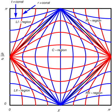
Figure 1: The Penrose diagram for dS spacetime covered by the coordinates corresponding to the negative curvature spatial foliation.

We are interested in effects of a spherical boundary with radius $r=r_{0}$ on the local characteristics of the vacuum state for a scalar field $\varphi(x)$ with curvature coupling parameter $\xi$. The corresponding field equation has the form

$$\left(\nabla_{\mu}\nabla^{\mu}+m^{2}+\xi R\right)\varphi=0,$$ (2.4)

where $\nabla_{\mu}$ is the covariant derivative operator and the Ricci scalar is given by $R=D\left(D+1\right)/\alpha^{2}$. On the sphere the field obeys the Robin boundary condition

$$\left(A-\delta_{\mathrm{(j)}}B\partial_{r}\right)\varphi(x)=0,\;r=r_{0},$$ (2.5)

where $\mathrm{j}=\mathrm{i}$ and $\mathrm{j}=\mathrm{e}$ correspond to the interior ($r\leq r_{0}$) and exterior ($r\geq r_{0}$) regions with $\delta_{\mathrm{(i)}}=1$ and $\delta_{\mathrm{(e)}}=-1$. It is of interest to have the radius of the sphere $r_{\mathrm{I}0}$ in inflationary coordinates. By using the relations (A.19), we can see that

$$r_{\mathrm{I}0}/\alpha=\coth r_{0}-\sqrt{\sinh^{-2}r_{0}+e^{-2t_{\mathrm{I}}/\alpha}}.$$ (2.6)

As seen, in inflationary coordinates the radius of the sphere is time-dependent. One has $r_{\mathrm{I}0}=0$ for $t_{\mathrm{I}}=0$. With increasing $t_{\mathrm{I}}$ the radius $r_{\mathrm{I}0}$ increases and in the limit $t_{\mathrm{I}}\rightarrow\infty$ it tends to the value $\lim_{t_{\mathrm{I}}\rightarrow\infty}r_{\mathrm{I}0}=\alpha\tanh(r_{0}/2)$.

The VEVs of the physical quantities bilinear in the field operator are obtained from the two-point functions or their derivatives in the coincidence limit of the arguments. As a two-point function we will consider the Hadamard function $G(x,x^{\prime})=\langle 0|\varphi(x)\varphi(x^{\prime})+\varphi(x^{\prime})\varphi(x)|0\rangle$, where $|0\rangle$ stands for the vacuum state and $x=\left(t,r,\vartheta,\phi\right)$. For the evaluation of the Hadamard function we will employ the mode sum formula

$$G(x,x^{\prime})=\sum_{\sigma}\left[\varphi_{\sigma}\left(x\right)\varphi_{\sigma}^{\ast}\left(x^{\prime}\right)+\varphi_{\sigma}\left(x^{\prime}\right)\varphi_{\sigma}^{\ast}\left(x\right)\right],$$ (2.7)

where $\{\varphi_{\sigma}\left(x\right),\varphi_{\sigma}^{\ast}\left(x^{\prime}\right)\}$ is a complete set of solutions to the classical field equation obeying the boundary condition and the collective index $\sigma$ specifies the quantum numbers. The symbol $\sum_{\sigma}$ includes the summation over discrete quantum numbers and the integration over the continuous ones. Given the Hadamard function, the VEVs of the field squared, $\langle 0|\varphi^{2}(x)|0\rangle\equiv\left\langle\varphi^{2}(x)\right\rangle$, and of the energy-momentum tensor, $\langle 0|T_{ik}(x)|0\rangle\equiv\left\langle T_{ik}(x)\right\rangle$, are found in the coincidence limit of the arguments as follows:

$$\left\langle\varphi^{2}(x)\right\rangle = \frac{1}{2}\underset{x^{\prime}\rightarrow x}{\lim}G\left(x,x^{\prime}\right),$$

$$\left\langle T_{ik}(x)\right\rangle = \frac{1}{2}\underset{x^{\prime}\rightarrow x}{\lim}\partial_{i^{\prime}}\partial_{k}G\left(x,x^{\prime}\right)+\left(\xi-\frac{1}{4}\right)g_{ik}\nabla_{p}\nabla^{p}\left\langle\varphi^{2}\right\rangle-\xi\nabla_{i}\nabla_{k}\left\langle\varphi^{2}\right\rangle-\xi R_{ik}\left\langle\varphi^{2}\right\rangle,$$ (2.8)

where $R_{ik}$ is the Ricci tensor. Of course, the expressions in the right-hand sides diverge and a renormalization is required. Here we are interested in the contributions to the VEVs induced by the spherical boundary. In the discussion below the corresponding contribution in the Hadamard function will be extracted explicitly. The divergences are determined by the local geometry and for points away from the sphere they are the same in the problems without and with spherical boundary. This means that for those points the renormalization in (2.8) is reduced to the one in the problem where the spherical boundary is absent.

As the first step we need to specify the mode functions $\varphi_{\sigma}\left(x\right)$. In accordance with the symmetry of the problem the solution of the field equation (2.4) can be presented in the form (for a discussion of the scalar field mode function in $D=3$ dS spacetime with negative curvature spatial sections see also [43, 44])

$$\varphi\left(x\right)=f\left(t/\alpha\right)g\left(r\right)Y\left(m_{p};\vartheta,\phi\right),$$ (2.9)

where $Y(m_{p};\vartheta,\phi)$ are hyperspherical harmonics of degree $l=0,1,2,\ldots$. For the set of quantum numbers $m_{p}$ one has $m_{p}=(m_{0}\equiv l,m_{1},\ldots,m_{n})$, with $m_{1},m_{2},\ldots,m_{n}$ being integers such that $-m_{n-1}\leqslant m_{n}\leqslant m_{n-1}$ and

$$0\leqslant m_{n-1}\leqslant m_{n-2}\leqslant\cdots\leqslant m_{1}\leqslant l.$$ (2.10)

The angular part in (2.9) obeys the equation

$$\Delta_{\vartheta,\phi}Y\left(m_{p};\vartheta,\phi\right)=-l\left(l+n\right)Y\left(m_{p};\vartheta,\phi\right),$$ (2.11)

with $\Delta_{\vartheta,\phi}$ being the Laplace operator on a unit sphere. Substituting (2.9) into the field equation we get separate equations for the functions $f(t/\alpha)$ and $g(r)$:

$$\frac{\partial_{\tau}\left[\sinh^{D}\tau\partial_{\tau}f\left(\tau\right)\right]}{\sinh^{D}\tau}+\left[m^{2}\alpha^{2}+\xi D\left(D+1\right)+\frac{\gamma^{2}}{\sinh^{2}\tau}\right]f\left(\tau\right) = 0,$$

$$\frac{\partial_{r}\left[\sinh^{D-1}r\partial_{r}g\left(r\right)\right]}{\sinh^{D-1}r}+\left[\gamma^{2}-\frac{l\left(l+n\right)}{\sinh^{2}r}\right]g\left(r\right) = 0,$$ (2.12)

where $\tau=t/\alpha$ and $\gamma^{2}$ is the separation constant.

The equations (2.12) have the same structure and the corresponding solutions are expressed in terms of the associated Legendre functions $P_{\nu}^{\mu}\left(u\right)$ and $Q_{\nu}^{\mu}\left(u\right)$ (for the properties of the associated Legendre functions see [45, 46]). The solutions are presented in the form

$$f\left(\tau\right) = \frac{X_{\nu}^{iz}\left(\cosh\tau\right)}{\sinh^{(D-1)/2}\tau},$$

$$g\left(r\right) = \frac{Z_{iz-1/2}^{-\mu}\left(\cosh r\right)}{\sinh^{D/2-1}r},$$ (2.13)

with the functions

$$X_{\nu}^{iz}\left(y\right) = d_{1}P_{\nu-1/2}^{iz}\left(y\right)+d_{2}Q_{\nu-1/2}^{iz}\left(y\right),$$

$$Z_{iz-1/2}^{-\mu}\left(u\right) = c_{1}P_{iz-1/2}^{-\mu}\left(u\right)+c_{2}Q_{iz-1/2}^{-\mu}\left(u\right),$$ (2.14)

and notations

$$\mu = l+\frac{D}{2}-1,$$

$$\nu = \sqrt{\frac{D^{2}}{4}-\xi D\left(D+1\right)-m^{2}\alpha^{2}}.$$ (2.15)

The separation constant is expressed in terms of $z$ as $\gamma^{2}=z^{2}+\left(D-1\right)^{2}/4$. The parameter $\nu$ can be either real or purely imaginary.

On the base of (2.13), the mode functions are presented in the form

$$\varphi_{\sigma}\left(x\right)=\frac{X_{\nu}^{iz}\left(\cosh(t/\alpha)\right)}{\sinh^{(D-1)/2}(t/\alpha)}\frac{Z_{iz-1/2}^{-\mu}\left(\cosh r\right)}{\sinh^{D/2-1}r}Y\left(m_{p};\vartheta,\phi\right),$$ (2.16)

where the set of quantum numbers is specified by $\sigma=(z,m_{p})$. The coefficients $c_{1},c_{2},d_{1},d_{2}$ in the linear combinations of the associated Legendre functions are determined by the choice of the vacuum state and by the boundary and normalization conditions. The latter is given by

$$\int d^{D}x\sqrt{\left|g\right|}\varphi_{\sigma}\left(x\right)\overleftrightarrow{\partial_{t}}\varphi_{\sigma^{\prime}}^{\ast}\left(x\right)=i\delta_{\sigma\sigma^{\prime}},$$ (2.17)

where $\delta_{\sigma\sigma^{\prime}}$ is understood as Kronecker delta for discrete quantum numbers and Dirac delta function for continuous ones. Note that we can also present the function $X_{\nu}^{iz}\left(y\right)$ as a linear combination of the functions $P_{\nu-1/2}^{\pm iz}\left(y\right)$:

$$X_{\nu}^{iz}\left(y\right)=\sum_{j=+,-}b_{j}P_{\nu-1/2}^{jiz}\left(y\right).$$ (2.18)

By using the relation between the functions $Q_{\nu-1/2}^{iz}\left(y\right)$ and $P_{\nu-1/2}^{\pm iz}\left(y\right)$, for the corresponding coefficients one gets

$$b_{+} = d_{1}-\frac{i\pi e^{-\pi z}}{2\sinh\left(\pi z\right)}d_{2},$$

$$b_{-} = \frac{i\pi e^{-\pi z}}{2\sinh\left(\pi z\right)}\frac{\Gamma\left(\nu+iz+1/2\right)}{\Gamma\left(\nu-iz+1/2\right)}d_{2},$$ (2.19)

where $\Gamma(x)$ is the gamma function. Note that one has the relation

$$P_{\nu^{\ast}-1/2}^{-iz}\left(y\right)=P_{\nu-1/2}^{-iz}\left(y\right),$$ (2.20)

for both real and purely imaginary $\nu$.

We impose an additional condition

$$W\left\{f\left(\tau\right),f^{\ast}\left(\tau\right)\right\}=f\left(\tau\right)\partial_{\tau}f^{\ast}\left(\tau\right)-\partial_{\tau}f\left(\tau\right)f^{\ast}\left(\tau\right)=\frac{i}{\sinh^{D}\tau},$$ (2.21)

on the function $f\left(\tau\right)$ in (2.13), where $W\left\{f_{1}\left(\tau\right),f_{2}\left(\tau\right)\right\}$ stands for the Wronskian. This imposes a constraint on the coefficients of the linear combination of the associated Legendre functions in the expression for the function $X_{\nu}^{iz}\left(y\right)$. In order to obtain that constraint it is convenient to employ the representation (2.18). By using (2.20) and the Wronskian

$$W\left\{P_{\nu-1/2}^{iz}\left(y\right),P_{\nu-1/2}^{-iz}\left(y\right)\right\}=\frac{2i}{\pi}\frac{\sinh\left(\pi z\right)}{y^{2}-1},$$ (2.22)

the following relation is obtained for the coefficients in (2.18):

$$\left|b_{+}\right|^{2}-\left|b_{-}\right|^{2}=\frac{\pi}{2\sinh\left(\pi z\right)}.$$ (2.23)

In deriving this relation we have assumed that $z$ is real. In the case of purely imaginary $z$ the condition (2.21) is reduced to

$$b_{+}b_{-}^{\ast}-b_{+}^{\ast}b_{-}=\frac{\pi}{2\sinh\left(\pi z\right)}.$$ (2.24)

Having the condition (2.21) and by taking into account the formula

$$\int d\Omega\,\,Y(m_{p};\vartheta,\phi)Y^{\ast}(m_{p}^{\prime};\vartheta,\phi)=N(m_{p})\delta_{m_{p}m_{p}^{\prime}},$$ (2.25)

for the integral over the angular coordinates, the normalization condition (2.17) is written in terms of the radial functions:

$$\int du\,Z_{iz-1/2}^{-\mu}\left(u\right)[Z_{iz^{\prime}-1/2}^{-\mu}\left(u\right)]^{\ast}=\frac{\alpha^{1-D}}{N\left(m_{p}\right)}\delta_{zz^{\prime}}.$$ (2.26)

Here, the integration goes over the region $[1,\cosh r_{0}]$ for the mode functions inside the sphere and over the region $[\cosh r_{0},\infty)$ for the exterior modes. The explicit expression for $N(m_{p})$ is not required in the following discussion and can be found, for example, in [47].

An alternative representation of the time-dependent part in the mode functions is obtained by using the relation

$$P_{\nu-1/2}^{\pm iz}\left(\cosh(t/\alpha)\right)=\frac{\sqrt{2/\pi}e^{i\nu\pi}Q_{\mp iz-1/2}^{-\nu}\left(\coth(t/\alpha)\right)}{\Gamma\left(1/2-\nu\mp iz\right)\sqrt{\sinh(t/\alpha)}},$$ (2.27)

between the associated Legendre functions. For the function in (2.16) this gives

$$X_{\nu}^{iz}\left(\cosh(t/\alpha)\right)=\frac{\sqrt{2/\pi}e^{i\nu\pi}}{\sqrt{\sinh(t/\alpha)}}\sum_{j=+,-}\frac{b_{j}Q_{-jiz-1/2}^{-\nu}\left(\coth(t/\alpha)\right)}{\Gamma\left(1/2-\nu-jiz\right)}.$$ (2.28)

Equivalently, we can use the formula

$$e^{i\pi\nu}Q_{\pm iz-1/2}^{-\nu}(y)=-\frac{\pi}{2\sin\left(\pi\nu\right)}\left[P_{iz-1/2}^{-\nu}(y)-\frac{\Gamma\left(\pm iz-\nu+1/2\right)}{\Gamma\left(\pm iz+\nu+1/2\right)}P_{iz-1/2}^{\nu}(y)\right],$$ (2.29)

in order to express the modes in terms of the functions $P_{iz-1/2}^{\pm\nu}(y)$:

$$X_{\nu}^{iz}\left(\cosh(t/\alpha)\right)=\frac{\sqrt{\pi/2}}{\sin\left(\pi\nu\right)}\sum_{j=+,-}jc_{j}\frac{P_{iz-1/2}^{j\nu}(\coth(t/\alpha))}{\sqrt{\sinh(t/\alpha)}},$$ (2.30)

with the coefficients

$$c_{\pm}=\sum_{j=+,-}\frac{b_{j}}{\Gamma\left(1/2\pm\nu-jiz\right)}.$$ (2.31)

3 Vacuum states

The coefficients in the linear combination (2.18) are related by (2.23) and (2.24) for modes with real and purely imaginary $z$, respectively. The remaining degree of freedom is fixed by the choice of the vacuum state. In order to discuss the vacuum states let us consider special and limiting cases. For a conformally coupled massless scalar field one has $\xi=\xi_{D}=(D-1)/(4D)$ and $\nu=1/2$. For the associated Legendre functions in the expressions of the scalar modes we get

$$P_{0}^{\pm iz}\left(\cosh\left(t/\alpha\right)\right)=\frac{e^{\mp iz\eta/\alpha}}{\Gamma\left(1\mp iz\right)},$$ (3.1)

and, hence,

$$X_{1/2}^{iz}\left(\cosh\left(t/\alpha\right)\right)=\sum_{j=+,-}\frac{b_{j}e^{-jiz\eta/\alpha}}{\Gamma\left(1-jiz\right)},$$ (3.2)

where the conformal time $\eta$ is defined by (2.2). The modes realizing the conformal vacuum are related to the mode functions $\varphi_{\sigma}^{\mathrm{(st)}}\left(x\right)$ in static spacetime with a negative constant curvature space (with the line element given by the expression in the square brackets of (2.3)) by the formula $\varphi_{\sigma}\left(x\right)=\Omega^{\left(1-D\right)/2}\varphi_{\sigma}^{\mathrm{(st)}}\left(x\right)$ with the conformal factor $\Omega^{2}=\sinh^{-2}\left(\eta/\alpha\right)$.

For a conformally coupled massless field the static spacetime positive energy mode functions are expressed as

$$\varphi_{\sigma}^{\mathrm{(st)}}(x)=\frac{Z_{iz-1/2}^{-\mu}\left(\cosh r\right)}{\sinh^{D/2-1}r}Y\left(m_{k};\vartheta,\phi\right)e^{-iz\eta/\alpha},$$ (3.3)

with the energy $E=z/\alpha\geq 0$. Comparing (3.3) with (3.2), we see that for the conformal vacuum the quantum number $z$ is real and $b_{-}=0$. The other coefficient $b_{+}$ is found from the relation (2.23):

$$\left|b_{+}\right|^{2}=\frac{\pi}{2\sinh\left(z\pi\right)}.$$ (3.4)

The corresponding mode functions in dS spacetime are given by

$$\varphi_{\sigma}\left(t,r,\vartheta,\phi\right)=\sinh^{\frac{D-1}{2}}\left(|\eta|/\alpha\right)e^{-iz\eta/\alpha}\frac{Z_{iz-1/2}^{-\mu}\left(\cosh r\right)}{\sinh^{D/2-1}r}Y\left(m_{p};\vartheta,\phi\right),$$ (3.5)

where we have used $1/\sinh(t/\alpha)=-\sinh\left(\eta/\alpha\right)$ and have excluded the factor $b_{+}/\Gamma\left(1-iz\right)$ by redefining the coefficients $c_{1}$ and $c_{2}$ in (2.14). For a massive field with general curvature coupling the mode functions corresponding to the conformal vacuum are obtained from (2.16) with $b_{-}=0$ and $b_{+}$ given by (3.4). The corresponding eigenvalues of the quantum number $z$ are real.

In order to discuss the adiabatic vacuum we introduce the function $h(\eta)$ of the conformal time in accordance with $h(\eta)=$ $\sinh^{(D-1)/2}(t/\alpha)f\left(t/\alpha\right)$, where the function $t=t(\eta)$ is given by (2.2). This function obeys the equation

$$\partial_{\eta}^{2}h\left(\eta\right)+\omega^{2}\left(z,\eta\right)h\left(\eta\right)=0,$$ (3.6)

with time-dependent frequency

$$\omega\left(z,\eta\right)=\frac{1}{\alpha}\left[z^{2}-\frac{\nu^{2}-1/4}{\sinh^{2}\left(\eta/\alpha\right)}\right]^{1/2}.$$ (3.7)

From here it follows that the limit $\eta\rightarrow-\infty$ corresponds to asymptotically static region (static in-region). In terms of the proper time $t$ this corresponds to the region $t/\alpha\ll 1$. In the zeroth adiabatic order, for the modes realizing the in-vacuum one has $h^{(0)}(\eta)\sim e^{-iz\eta/\alpha}$, $\eta\rightarrow-\infty$. Let us consider the behavior of the mode functions (2.16) in that region. By using the asymptotics for the associated Legendre functions one gets

$$X_{\nu}^{iz}\left(\cosh(t/\alpha)\right)\approx\sum_{j=+,-}\frac{b_{j}e^{-jiz\eta/\alpha}}{\Gamma\left(1-jiz\right)},\;t/\alpha\ll 1.$$ (3.8)

From here it follows that for the mode functions that are reduced to the positive energy modes in static spacetime we should take $b_{-}=0$ and, hence, the conformal and adiabatic vacua coincide. The corresponding state is also known as hyperbolic vacuum. Note that the latter is different from the maximally symmetric Bunch-Davies vacuum state (for the relation between the hyperbolic and Bunch-Davies vacua in the special case of $D=3$ boundary-free dS spacetime see also [43, 44]).

Now let us consider the flat spacetime limit $\alpha\rightarrow\infty$. The line element takes the form

$$ds^{2}=dt^{2}-t^{2}(dr^{2}+\sinh^{2}rd\Omega_{D-1}^{2}),$$ (3.9)

which corresponds to the Milne universe. In order to find the limiting form of the scalar mode functions (2.16) we note that in the limit under consideration $\nu\approx im\alpha$ and $|\nu|$ is large. We can use the relation

$$\underset{\alpha\rightarrow\infty}{\lim}\left[\left(m\alpha\right)^{\pm iz}P_{im\alpha-1/2}^{\mp iz}\left(\cosh(t/\alpha)\right)\right]=J_{\pm iz}\left(mt\right),$$ (3.10)

where $J_{\nu}(x)$ is the Bessel function. For the scalar modes one gets $\lim_{\alpha\rightarrow\infty}\varphi_{\sigma}\left(x\right)=\varphi_{\sigma}^{\mathrm{(Milne)}}\left(x\right)$, where the mode functions in the Milne universe are given by

$$\varphi_{\sigma}^{\mathrm{(Milne)}}\left(x\right)=c\frac{\tilde{b}_{+}J_{-iz}(mt)+\tilde{b}_{-}J_{iz}(mt)}{t^{\left(D-1\right)/2}}\frac{P_{iz-1/2}^{-\mu}\left(\cosh r\right)}{\sinh^{D/2-1}r}Y(m_{p};\vartheta,\phi),$$ (3.11)

with $|\tilde{b}_{j}|=|b_{j}|$ and

$$|c|^{2}=\frac{z\sinh(\pi z)}{\pi N\left(m_{p}\right)}|\Gamma(iz+\mu+1/2)|.$$ (3.12)

These mode functions have been discussed in [48]. In the Milne universe the conformal and adiabatic vacua are different. The conformal vacuum corresponds to the special case $\tilde{b}_{-}=0$ with $|\tilde{b}_{+}|^{2}=\pi/[2\sinh\left(\pi z\right)]$ and for the adiabatic vacuum in the Milne universe

$$\tilde{b}_{+}=\frac{\sqrt{\pi}e^{\pi z/2}}{2\sinh\left(\pi z\right)},\;\tilde{b}_{-}=-\tilde{b}_{+}e^{-\pi z}.$$ (3.13)

For the adiabatic vacuum the time-dependence in the corresponding mode function (3.11) is expressed in terms of the function $t^{\left(1-D\right)/2}H_{iz}^{\left(2\right)}\left(mt\right)$ with the Hankel function $H_{iz}^{\left(2\right)}\left(x\right)$.

4 Hadamard function

Having specified the general structure of the mode functions we turn to the construction of the Hadamard function in accordance with (2.7). The boundary-free, exterior and interior geometries will be considered separately.

4.1 Boundary-free geometry

We start with the problem where the sphere is absent. For the modes regular at the origin $r=0$ one should take $c_{2}=0$ in (2.14) and the corresponding mode functions take the form

$$\varphi_{\sigma}^{(0)}\left(x\right)=C_{0}\frac{X_{\nu}^{iz}\left(\cosh(t/\alpha)\right)}{\sinh^{(D-1)/2}(t/\alpha)}\frac{P_{iz-1/2}^{-\mu}\left(\cosh r\right)}{\sinh^{D/2-1}r}Y\left(m_{p};\vartheta,\phi\right),$$ (4.1)

with $0\leq r<\infty$. The spectrum of the quantum number $z$ is continuous, $0\leq z<\infty$, and in the right-hand side of the normalization condition (2.26) we take $\delta_{zz^{\prime}}=\delta(z-z^{\prime})$ with the integration range $u\in[1,\infty)$. By using the result

$$\int_{1}^{\infty}duP_{iz-1/2}^{-\mu}\left(u\right)P_{iz^{\prime}-1/2}^{-\mu}\left(u\right)=\frac{\pi\delta\left(z-z^{\prime}\right)}{z\sinh\left(\pi z\right)\left|\Gamma\left(iz+\mu+1/2\right)\right|^{2}},$$ (4.2)

for the normalization coefficient one gets

$$\left|C_{0}\right|^{2}=\frac{z\sinh\left(\pi z\right)}{\pi N\left(m_{p}\right)}\frac{\left|\Gamma\left(\mu+iz+1/2\right)\right|^{2}}{\alpha^{D-1}}.$$ (4.3)

Substituting the mode functions (4.1) into the corresponding mode sum formula (2.7) and by using the addition theorem

$$\sum_{m_{k}}\frac{Y\left(m_{p};\vartheta,\phi\right)}{N\left(m_{p}\right)}Y^{\ast}\left(m_{p};\vartheta^{\prime},\phi^{\prime}\right)=\frac{2l+n}{nS_{D}}C_{l}^{n/2}\left(\cos\theta\right),$$ (4.4)

for spherical harmonics, for the Hadamard function in the boundary-free geometry we find

$$G_{0}(x,x^{\prime}) = \frac{2\alpha^{1-D}}{\pi nS_{D}}\overset{\infty}{\sum_{l=0}}\mu C_{l}^{n/2}\left(\cos\theta\right)\int_{0}^{\infty}dz\text{\thinspace}z\sinh\left(\pi z\right)\left|\Gamma\left(\mu+iz+1/2\right)\right|^{2}$$ (4.5)

$$\times\frac{X_{\nu}^{iz}\left(y\right)\left[X_{\nu}^{iz}\left(y^{\prime}\right)\right]^{\ast}+X_{\nu}^{iz}\left(y^{\prime}\right)\left[X_{\nu}^{iz}\left(y\right)\right]^{\ast}}{\left[\sinh(t/\alpha)\sinh(t^{\prime}/\alpha)\right]^{\frac{D-1}{2}}}\frac{P_{iz-1/2}^{-\mu}\left(u\right)P_{iz-1/2}^{-\mu}\left(u^{\prime}\right)}{\left(\sinh r\sinh r^{\prime}\right)^{\frac{D}{2}-1}},$$

with $\mu$ defined in (2.15) and

$$y = \cosh(t/\alpha),\;y^{\prime}=\cosh(t^{\prime}/\alpha),$$

$$u = \cosh r,\;u^{\prime}=\cosh r^{\prime}.$$ (4.6)

In this expression, $S_{D}=2\pi^{D/2}/\Gamma(D/2)$ is the surface area of the unit sphere in $D$-dimensional space, $C_{l}^{n/2}(\cos\theta)$ is the Gegenbauer polynomial and $\theta$ is the angle between the directions determined by $(\vartheta,\phi)$ and $(\vartheta^{\prime},\phi^{\prime})$.

For the hyperbolic vacuum

$$X_{\nu}^{iz}\left(y\right)=\sqrt{\frac{\pi}{2\sinh\left(\pi z\right)}}P_{\nu-1/2}^{iz}\left(y\right),$$ (4.7)

and the function (4.5) is reduced to

$$G_{0}\left(x,x^{\prime}\right) = \frac{\alpha^{1-D}}{nS_{D}}\sum_{l=0}^{\infty}\mu C_{l}^{n/2}\left(\cos\theta\right)\int_{0}^{\infty}dz\,z\left|\Gamma\left(\mu+iz+1/2\right)\right|^{2}$$ (4.8)

$$\times\frac{P_{iz-1/2}^{-\mu}\left(u\right)P_{iz-1/2}^{-\mu}\left(u^{\prime}\right)}{\left(\sinh r\sinh r^{\prime}\right)^{\frac{D}{2}-1}}\frac{\sum_{j=+,-}P_{\nu-1/2}^{jiz}\left(y\right)P_{\nu-1/2}^{-jiz}\left(y^{\prime}\right)}{\left[\sinh(t/\alpha)\sinh(t^{\prime}/\alpha)\right]^{\frac{D-1}{2}}}.$$

The further transformation of the Hadamard function in the boundary-free geometry is presented in Appendix B. In particular, the corresponding expression for the hyperbolic vacuum is obtained from (B.3) with the function $X_{\nu}^{ix}\left(y\right)$ from (4.7):

$$G_{0}\left(x,x^{\prime}\right) = \frac{\alpha^{1-D}}{2(2\pi)^{D/2}}\int_{0}^{\infty}dz\,z\left|\Gamma\left(\frac{D-1}{2}+iz\right)\right|^{2}$$ (4.9)

$$\times\frac{\sum_{j=+,-}P_{\nu-1/2}^{jiz}\left(y\right)P_{\nu-1/2}^{-jiz}\left(y^{\prime}\right)}{\left[\sinh(t/\alpha)\sinh(t^{\prime}/\alpha)\right]^{\frac{D-1}{2}}}\frac{P_{iz-1/2}^{1-D/2}\left(\bar{u}\right)}{\left(\bar{u}^{2}-1\right)^{\frac{D-2}{4}}},$$

where

$$\bar{u}=\cosh r\cosh r^{\prime}-\sinh r\sinh r^{\prime}\cos\theta.$$ (4.10)

In the limit $\alpha\rightarrow\infty$, by using the relation (3.10), from (4.9) we obtain the Hadamard function for the conformal vacuum in the Milne universe:

$$G_{0}^{\mathrm{(Milne)}}\left(x,x^{\prime}\right) = \frac{(tt^{\prime})^{(1-D)/2}}{2(2\pi)^{D/2}}\int_{0}^{\infty}dz\,z\left|\Gamma\left(\frac{D-1}{2}+iz\right)\right|^{2}$$ (4.11)

$$\times\frac{P_{iz-1/2}^{1-D/2}\left(\bar{u}\right)}{\left(\bar{u}^{2}-1\right)^{\frac{D-2}{4}}}\sum_{j=+,-}J_{jiz}\left(mt\right)J_{-jiz}\left(mt^{\prime}\right).$$

It can be checked that this formula is obtained from the corresponding expression in [48] by making use of the addition theorem (B.2).

4.2 Region outside the sphere

In the region outside the sphere, $r>r_{0}$, the mode functions have the form (2.16) where the function $Z_{iz-1/2}^{-\mu}\left(u\right)$ is given by (2.14). For the exterior region it is more convenient to take the linear combination of the functions $Q_{iz-1/2}^{-\mu}\left(u\right)$ and $Q_{-iz-1/2}^{-\mu}\left(u\right)$ by using the relation

$$P_{iz-1/2}^{-\mu}\left(u\right)=\frac{ie^{i\mu\pi}}{\pi\sinh\left(\pi z\right)}\sum_{j=+,-}j\cos\left[\pi\left(\mu-jiz\right)\right]Q_{jiz-1/2}^{-\mu}\left(u\right).$$ (4.12)

For the modes with real values of $z$ the ratio of the coefficients in that combination is determined by the boundary condition (2.5) and is expressed as $-\bar{Q}_{-iz-1/2}^{-\mu}\left(u_{0}\right)/\bar{Q}_{iz-1/2}^{-\mu}\left(u_{0}\right)$ with

$$u_{0}=\cosh r_{0}.$$ (4.13)

Here and below, for a given function $F(u)$, the notation with bar is defined as

$$\bar{F}\left(u\right)=\left[B\left(u\right)\partial_{u}+A\left(u\right)\right]F\left(u\right),$$ (4.14)

where the functions $A(u)$ and $B(u)$ are expressed in terms of the Robin coefficients:

$$A\left(u\right) = A\sqrt{u^{2}-1}+\left(\frac{D}{2}-1\right)\delta_{\mathrm{(j)}}Bu,$$

$$B\left(u\right) = -\delta_{\mathrm{(j)}}B\left(u^{2}-1\right).$$ (4.15)

Here, $\mathrm{j=e}$ and $\mathrm{j=i}$ for the regions outside and inside the sphere, respectively, with $\delta_{\mathrm{(e)}}=-1$ and $\delta_{\mathrm{(i)}}=1$. For the corresponding scalar modes one obtains

$$\varphi_{\sigma}^{\mathrm{(e)}}\left(x\right)=C_{\mathrm{(e)}}\frac{X_{\nu}^{iz}\left(\cosh(t/\alpha)\right)}{\sinh^{(D-1)/2}(t/\alpha)}\frac{W_{iz}^{-\mu}\left(\cosh r\right)}{\sinh^{D/2-1}r}Y\left(m_{p};\vartheta,\phi\right),$$ (4.16)

where we have defined the function

$$W_{iz}^{-\mu}\left(u\right)=\bar{Q}_{iz-1/2}^{-\mu}\left(u_{0}\right)Q_{-iz-1/2}^{-\mu}\left(u\right)-\bar{Q}_{-iz-1/2}^{-\mu}\left(u_{0}\right)Q_{iz-1/2}^{-\mu}\left(u\right).$$ (4.17)

Similar to the case of the boundary-free geometry, in the exterior region the eigenvalues for $z$ are continuous.

From (2.26) the following orthonormalization condition is obtained in terms of the function (4.17):

$$\left|C_{\mathrm{(e)}}\right|^{2}\int_{u_{0}}^{\infty}duW_{iz}^{-\mu}\left(u\right)[W_{iz^{\prime}}^{-\mu}\left(u\right)]^{\ast}=\frac{\delta\left(z-z^{\prime}\right)}{\alpha^{D-1}N\left(m_{p}\right)}.$$ (4.18)

The $u$-integral diverges in the upper limit for $z=z^{\prime}$ and, hence, the contribution from the integration range with large $u$ dominates. So, in order to evaluate this integral, we can replace the associated Legendre functions $Q_{\pm iz-1/2}^{-\mu}\left(u\right)$ in (4.17) by their asymptotic expressions for large values of the argument:

$$Q_{\pm iz-1/2}^{-\mu}\left(u\right)\approx\sqrt{\pi}e^{-i\mu\pi}\frac{\Gamma\left(1/2\pm iz-\mu\right)}{\Gamma\left(1\pm iz\right)}\frac{e^{\mp iz\ln\left(2u\right)}}{\sqrt{2u}}.$$ (4.19)

This leads to the following result

$$\left|C_{\mathrm{(e)}}\right|^{2}=\frac{z\left|\Gamma\left(1/2+iz-\mu\right)\bar{Q}_{iz-1/2}^{-\mu}\left(u_{0}\right)\right|^{-2}}{\pi\alpha^{D-1}N\left(m_{p}\right)\sinh\left(\pi z\right)},$$ (4.20)

for the normalization coefficient.

With the mode functions (4.16), from the mode sum formula (2.7), by using the addition theorem (4.4), the following representation is obtained for the Hadamard function in the exterior region:

$$G(x,x^{\prime}) = \frac{2\alpha^{1-D}}{\pi nS_{D}}\frac{\left(\sinh r\sinh r^{\prime}\right)^{1-\frac{D}{2}}}{\left[\sinh(t/\alpha)\sinh(t^{\prime}/\alpha)\right]^{\frac{D-1}{2}}}\sum_{l=0}^{\infty}\mu C_{l}^{n/2}\left(\cos\theta\right)\int_{0}^{\infty}dz\,z$$ (4.21)

$$\times\frac{X_{\nu}^{iz}\left(y\right)W_{iz}^{-\mu}\left(u\right)[X_{\nu}^{iz}\left(y^{\prime}\right)W_{iz}^{-\mu}\left(u^{\prime}\right)]^{\ast}+\left\{(y,u)\rightleftarrows(y^{\prime},u^{\prime})\right\}}{\sinh\left(\pi z\right)\left|\Gamma\left(1/2+iz-\mu\right)\right|^{2}\left|\bar{Q}_{iz-1/2}^{-\mu}\left(u_{0}\right)\right|^{2}}.$$

We can also write this expression in terms of the function

$$Y_{iz-1/2}^{-\mu}\left(u\right)=\bar{Q}_{iz-1/2}^{-\mu}\left(u_{0}\right)P_{iz-1/2}^{-\mu}\left(u\right)-\bar{P}_{iz-1/2}^{-\mu}\left(u_{0}\right)Q_{iz-1/2}^{-\mu}\left(u\right),$$ (4.22)

by using the relation

$$W_{iz}^{-\mu}\left(u\right)=\frac{i\pi e^{-i\mu\pi}\sinh\left(\pi z\right)}{\cos\left[\pi\left(\mu+iz\right)\right]}Y_{iz-1/2}^{-\mu}\left(u\right).$$ (4.23)

The corresponding expression takes the form

$$G(x,x^{\prime}) = \frac{2\alpha^{1-D}}{\pi nS_{D}}\overset{\infty}{\sum_{l=0}}\mu C_{l}^{n/2}\left(\cos\theta\right)\int_{0}^{\infty}dz\,z\sinh\left(\pi z\right)\frac{\left|\Gamma\left(\mu+iz+1/2\right)\right|^{2}}{\left|\bar{Q}_{iz-1/2}^{-\mu}\left(u_{0}\right)\right|^{2}}$$ (4.24)

$$\times\frac{X_{\nu}^{iz}\left(y\right)Y_{iz-1/2}^{-\mu}\left(u\right)[X_{\nu}^{iz}\left(y^{\prime}\right)Y_{iz-1/2}^{-\mu}\left(u^{\prime}\right)]^{\ast}+\left\{(y,u)\rightleftarrows(y^{\prime},u^{\prime})\right\}}{\left[\sinh(t/\alpha)\sinh(t^{\prime}/\alpha)\right]^{\frac{D-1}{2}}\left(\sinh r\sinh r^{\prime}\right)^{\frac{D}{2}-1}}.$$

Depending on the ratio of the coefficients in the Robin boundary condition, in addition to the modes with real $z$, one can have exterior modes with purely imaginary $z=\pm i\chi$, $\chi>0$. The radial dependence of the corresponding normalizable mode functions is expressed in terms of the function $Q_{\chi-1/2}^{-\mu}(u)/\sinh^{D/2-1}r$ and they correspond to bound states. From the boundary condition (2.5) we get the equation $\bar{Q}_{\chi-1/2}^{-\mu}(u_{0})=0$ that determines the eigenvalues for $\chi$. As it has been already discussed in [49], one has a critical value $\beta_{l}^{\mathrm{(e)}}(u_{0})$ for the ratio $\beta=A/B$ such that there are no roots for this equation in the range $\beta\leq\beta_{l}^{\mathrm{(e)}}(u_{0})$ and a single root exists in the region $\beta>\beta_{l}^{\mathrm{(e)}}(u_{0})$. In [49] it has been shown that $\beta_{l}^{\mathrm{(e)}}(u_{0})$ is an increasing function of $l$ and a decreasing function of $u_{0}$. In addition, we have $\beta_{l}^{\mathrm{(e)}}(u_{0})\geq(D-1)/2$. For the hyperbolic vacuum the corresponding function $X_{\nu}^{iz}\left(y\right)$ is given by (4.7) and the allowed values for $z$ are real. In order to exclude the modes with $z=\pm i\chi$, it will be assumed that $\beta\leq\beta_{0}^{\mathrm{(e)}}(u_{0})$. Note that the Neumann boundary condition ($\beta=0$) belongs to this range. In the special case $D=3$, by using

$$Q_{\chi-1/2}^{-1/2}(u_{0})=-i\frac{\sqrt{\pi/2}e^{-\chi r_{0}}}{\chi\sqrt{\sinh r_{0}}},$$ (4.25)

for the bound state corresponding to the mode $l=0$ we get $\chi=\beta-\coth r_{0}$. From here it follows that $\beta_{0}^{\mathrm{(e)}}(u_{0})=\coth r_{0}$ for $D=3$.

We are interested in the effects of the sphere on the properties of the hyperbolic vacuum. The corresponding Hadamard function outside the sphere is given by (4.24) with the function (4.7). By taking into account the expression (4.8) for the boundary-free geometry, the corresponding sphere-induced contribution $G_{\mathrm{s}}\left(x,x^{\prime}\right)=G\left(x,x^{\prime}\right)-G_{0}\left(x,x^{\prime}\right)$ is presented as

$$G_{\mathrm{s}}\left(x,x^{\prime}\right) = \frac{\alpha^{1-D}}{nS_{D}}\overset{\infty}{\sum_{l=0}}\mu C_{l}^{n/2}\left(\cos\theta\right)\int_{0}^{\infty}dz\,z\left|\Gamma\left(\mu+iz+1/2\right)\right|^{2}$$ (4.26)

$$\times\frac{P_{\nu-1/2}^{iz}\left(y\right)P_{\nu-1/2}^{-iz}\left(y^{\prime}\right)U_{iz-1/2}^{-\mu}(u,u^{\prime})+\left\{(y,u)\rightleftarrows(y^{\prime},u^{\prime})\right\}}{\left[\sinh(t/\alpha)\sinh(t^{\prime}/\alpha)\right]^{\frac{D-1}{2}}\left(\sinh r\sinh r^{\prime}\right)^{\frac{D}{2}-1}},$$

with the notation

$$U_{iz-1/2}^{-\mu}(u,u^{\prime})=\frac{Y_{iz-1/2}^{-\mu}\left(u\right)[Y_{iz-1/2}^{-\mu}\left(u^{\prime}\right)]^{\ast}}{\left|\bar{Q}_{iz-1/2}^{-\mu}\left(u_{0}\right)\right|^{2}}-P_{iz-1/2}^{-\mu}\left(u\right)P_{iz-1/2}^{-\mu}\left(u^{\prime}\right).$$ (4.27)

For the further transformation of the function (4.26) it is convenient to use the relation

$$U_{iz-1/2}^{-\mu}(u,u^{\prime})=\frac{-ie^{i\mu\pi}}{\pi\sinh\left(\pi z\right)}\underset{j=+,-}{\sum}j\cos\left[\pi\left(\mu-jiz\right)\right]\frac{\bar{P}_{iz-1/2}^{-\mu}\left(u_{0}\right)}{\bar{Q}_{jiz-1/2}^{-\mu}\left(u_{0}\right)}Q_{jiz-1/2}^{-\mu}\left(u\right)Q_{jiz-1/2}^{-\mu}\left(u^{\prime}\right).$$ (4.28)

The term with $j=-$ ($j=+$) exponentially decreases in the upper (lower) half-plane of the complex variable $z$ in the limit $\mathrm{Im}\,z\rightarrow+\infty$ ($\mathrm{Im}\,z\rightarrow-\infty$). On the base of these properties, in (4.26), with substitution (4.28), we can rotate the contour of the integration in the complex plane $z$ by the angles $\pi/2$ and $-\pi/2$ for the terms with $j=-$ and $j=+$, respectively. This leads to the representation

$$G_{\mathrm{s}}\left(x,x^{\prime}\right) = -\frac{2\alpha^{1-D}}{nS_{D}}\overset{\infty}{\sum_{l=0}}\mu C_{l}^{n/2}\left(\cos\theta\right)\int_{0}^{\infty}dz\,\frac{ze^{-i\mu\pi}}{\sin\left(\pi z\right)}\frac{\bar{P}_{z-1/2}^{-\mu}\left(u_{0}\right)}{\bar{Q}_{z-1/2}^{\mu}\left(u_{0}\right)}$$ (4.29)

$$\times\frac{Q_{z-1/2}^{\mu}\left(u\right)Q_{z-1/2}^{\mu}\left(u^{\prime}\right)}{\left(\sinh r\sinh r^{\prime}\right)^{\frac{D}{2}-1}}\frac{\sum_{j=+,-}P_{\nu-1/2}^{-jz}\left(y\right)P_{\nu-1/2}^{jz}\left(y^{\prime}\right)}{\left[\sinh(t/\alpha)\sinh(t^{\prime}/\alpha)\right]^{\frac{D-1}{2}}}.$$

Hence, the Hadamard function in the region outside the sphere is presented as

$$G\left(x,x^{\prime}\right)=G_{0}\left(x,x^{\prime}\right)+G_{\mathrm{s}}\left(x,x^{\prime}\right),$$ (4.30)

where the boundary-free contribution for the hyperbolic vacuum is given by (4.9). In the flat spacetime limit, corresponding to $\alpha\rightarrow\infty$, by using the relation

$$\lim_{\alpha\rightarrow\infty}\left[P_{\nu-1/2}^{-jz}\left(y\right)P_{\nu-1/2}^{jz}\left(y^{\prime}\right)\right]=J_{jz}(mt)J_{-jz}(mt^{\prime}),$$ (4.31)

from (4.29) the boundary-induced Hadamard function is obtained outside the sphere in the Milne universe [48].

4.3 Hadamard function inside the sphere

For the interior region, $r<r_{0}$, the regularity condition at the sphere center fixes $c_{2}=0$ in (2.14). The corresponding mode functions are expressed as

$$\varphi_{\sigma}^{\mathrm{(i)}}\left(t,r,\vartheta,\phi\right)=C_{\mathrm{(i)}}\frac{X_{\nu}^{iz}\left(\cosh(t/\alpha)\right)}{\sinh^{(D-1)/2}(t/\alpha)}\frac{P_{iz-1/2}^{-\mu}\left(\cosh r\right)}{\sinh^{D/2-1}r}Y\left(m_{p};\vartheta,\phi\right).$$ (4.32)

From the boundary condition (2.5) with $\mathrm{j}=\mathrm{i}$ we obtain the equation that determines the allowed values of the quantum number $z$:

$$\bar{P}_{iz-1/2}^{-\mu}(u_{0})=0,$$ (4.33)

with $u_{0}$ defined by (4.13). For the region under consideration the notation with bar in (4.33) is defined by (4.14) where now $\delta_{\mathrm{(j)}}=\delta_{\mathrm{(i)}}=1$ in (4.15). Hence, unlike the exterior region, inside the sphere the eigenvalues of $z$ form a discrete set. The positive solutions of the eigenvalue equation (4.33) we will denote as $z=z_{k}$, $k=1,2,\ldots$, assuming that $z_{k+1}>z_{k}$. These solutions do not depend on the curvature coupling parameter and on the field mass. In the special case $D=3$, by taking into account that

$$P_{iz-1/2}^{-1/2}\left(u_{0}\right)=\sqrt{\frac{2}{\pi}}\frac{\sin\left(zr_{0}\right)}{z\sqrt{\sinh r_{0}}},$$ (4.34)

the eigenvalue equation for the mode $l=0$ is simplified to

$$\left(\beta+\coth r_{0}\right)\sin\left(zr_{0}\right)/z=\cos\left(zr_{0}\right),$$ (4.35)

with the notation $\beta=A/B$.

The normalization coefficient $C_{\mathrm{(i)}}$ in (4.32) is determined by the condition (2.26) with $Z_{iz-1/2}^{-\mu}(u)=C_{\mathrm{(i)}}P_{iz-1/2}^{-\mu}\left(u\right)$, $z=z_{k}$, where the integration goes over the region $[1,u_{0}]$ and in the right-hand side $\delta_{zz^{\prime}}=\delta_{kk^{\prime}}$. The corresponding procedure is similar to that considered in [49]. By using the integral

$$\int_{1}^{u_{0}}du\,\left[P_{iz-1/2}^{\mu}\left(u\right)\right]^{2}=\frac{u_{0}^{2}-1}{2z}\left[\partial_{z}P_{iz-1/2}^{-\mu}\left(u_{0}\right)\partial_{u}P_{iz-1/2}^{-\mu}\left(u_{0}\right)-P_{iz-1/2}^{-\mu}\left(u_{0}\right)\partial_{z}\partial_{u}P_{iz-1/2}^{-\mu}\left(u_{0}\right)\right],$$ (4.36)

and the eigenvalue equation (4.33), we can show that

$$\left|C_{\mathrm{(i)}}\right|^{2}=\frac{2\alpha^{1-D}e^{i\mu\pi}z}{\pi N\left(m_{p}\right)}\left|\Gamma\left(\mu+iz+1/2\right)\right|^{2}T_{\mu}\left(z,u_{0}\right),$$ (4.37)

with $z=z_{k}$. Here we have introduced the notation

$$T_{\mu}\left(z,u\right)=\frac{\bar{Q}_{iz-1/2}^{-\mu}\left(u\right)}{\partial_{z}\bar{P}_{iz-1/2}^{-\mu}\left(u\right)}\cos\left[\pi\left(\mu-iz\right)\right].$$ (4.38)

With (4.37), the scalar mode functions inside the sphere are completely determined. Substituting the modes (4.32) into the mode sum (2.7) and making use of (4.4), the Hadamard function inside the sphere is presented in the form

$$G(x,x^{\prime}) = \frac{4\alpha^{1-D}}{\pi nS_{D}}\sum_{l=0}^{\infty}\mu C_{l}^{n/2}\left(\cos\theta\right)e^{i\mu\pi}\sum_{k=1}^{\infty}T_{\mu}\left(z,u_{0}\right)z\left|\Gamma\left(\mu+iz+1/2\right)\right|^{2}$$ (4.39)

$$\left.\times\frac{X_{\nu}^{iz}\left(y\right)\left[X_{\nu}^{iz}\left(y^{\prime}\right)\right]^{\ast}+X_{\nu}^{iz}\left(y^{\prime}\right)\left[X_{\nu}^{iz}\left(y\right)\right]^{\ast}}{\left[\sinh(t/\alpha)\sinh(t^{\prime}/\alpha)\right]^{\frac{D-1}{2}}}\frac{P_{iz-1/2}^{-\mu}\left(u\right)P_{iz-1/2}^{-\mu}\left(u^{\prime}\right)}{\left(\sinh r\sinh r^{\prime}\right)^{\frac{D}{2}-1}}\right|_{z=z_{k}}.$$

As in the previous discussion for the exterior region, we will assume that the field is prepared in the hyperbolic vacuum state with the function (4.7). It has been already emphasized that for the hyperbolic vacuum the eigenvalues of the quantum number $z$ are real. However, depending on the ratio $\beta=A/B$, the eigenvalue equation (4.33) may have purely imaginary roots. The conditions for the presence of those roots have been specified in [49]. For given values of $u_{0}$ and $l$ there exists a critical value of $\beta$, denoted here by $\beta_{l}^{\mathrm{(i)}}(u_{0})$, such that all the roots are real for $\beta\leq\beta_{l}^{\mathrm{(i)}}(u_{0})$ and a pair of purely imaginary roots $z_{\pm}=\pm i|z_{\pm}|$ appears for $\beta>\beta_{l}^{\mathrm{(i)}}(u_{0})$. For the critical value one has $\beta_{l}^{\mathrm{(i)}}(u_{0})>-(D-1)/2$ and it is an increasing function of $l$ and a decreasing function of $u_{0}$. For the critical values of the Robin coefficient in the exterior and interior regions one has the relation $\beta_{l}^{\mathrm{(e)}}(u_{0})>\beta_{l}^{\mathrm{(i)}}(u_{0})$. In the case $D=3$ from (4.35) we get

$$\beta_{0}^{\mathrm{(i)}}(u_{0})=\frac{1}{r_{0}}-\coth r_{0}.$$ (4.40)

In the discussion below, for the interior region we will assume the values of $\beta$ in the range $\beta\leq\beta_{0}^{\mathrm{(i)}}(u_{0})$, where all the roots of the equation (4.33) are real.

For the Hadamard function corresponding to the hyperbolic vacuum we get the representation

$$G(x,x^{\prime}) = \frac{2\alpha^{1-D}}{nS_{D}}\sum_{l=0}^{\infty}\mu C_{l}^{n/2}\left(\cos\theta\right)e^{i\mu\pi}\sum_{k=1}^{\infty}zT_{\mu}\left(z,u_{0}\right)\frac{\left|\Gamma\left(\mu+iz+1/2\right)\right|^{2}}{\sinh\left(\pi z\right)}$$ (4.41)

$$\left.\times\frac{P_{iz-1/2}^{-\mu}\left(u\right)P_{iz-1/2}^{-\mu}\left(u^{\prime}\right)}{\left(\sinh r\sinh r^{\prime}\right)^{\frac{D}{2}-1}}\frac{\sum_{j=+,-}P_{\nu-1/2}^{jiz}\left(y\right)P_{\nu-1/2}^{-jiz}\left(y^{\prime}\right)}{\left[\sinh(t/\alpha)\sinh(t/\alpha)^{\prime}\right]^{\frac{D-1}{2}}}\right|_{z=z_{k}},$$

where the relation (2.20) has been used. The summation in this formula goes over the eigenvalues $z_{k}$ that are defined implicitly, as roots of the equation (4.33). A more convenient representation is found by using the formula [48]

$$\sum_{k=1}^{\infty}T_{\mu}\left(z_{k},w\right)h\left(z_{k}\right) = \frac{e^{-i\mu\pi}}{2}\int_{0}^{\infty}dx\,\sinh\left(\pi x\right)h\left(x\right)$$ (4.42)

$$+\sum_{k}\cos\left[\pi\left(\mu-x_{k}\right)\right]\frac{\bar{Q}_{x_{k}-1/2}^{-\mu}\left(w\right)}{\bar{P}_{x_{k}-1/2}^{-\mu}\left(w\right)}\sum_{j=+,-}\mathrm{Res}_{z=jix_{k}}h(z)$$

$$-\frac{1}{2\pi}\int_{0}^{\infty}dx\,\frac{\bar{Q}_{x-1/2}^{-\mu}\left(w\right)}{\bar{P}_{x-1/2}^{-\mu}\left(w\right)}\cos\left[\pi\left(x-\mu\right)\right]\sum_{j=+,-}h\left(xe^{j\pi i/2}\right),$$

with a function $h(z)$ analytic in the half-plane $\mathrm{Re}\,z>0$. In (4.42), the points $\pm ix_{k}$ are possible poles of the function $h(z)$ on the imaginary axis. In the presence of these poles, it is assumed that the last integral is convergent in the sense of the principal value. The corresponding formula in the case when the poles on the imaginary axis are absent has been derived in [49, 50] by using the generalized Abel-Plana formula [51]. Additional conditions on the function $h(z)$ can be found in those references. The function $h(z)$ corresponding to the representation (4.41) of the Hadamard function is real for real values of $z$ and is expressed as

$$h\left(z\right)=z\frac{\Gamma\left(\mu+iz+1/2\right)}{\sinh\left(\pi z\right)}\Gamma\left(\mu-iz+1/2\right)P_{iz-1/2}^{-\mu}\left(u\right)P_{iz-1/2}^{-\mu}\left(u^{\prime}\right)\sum_{j=+,-}P_{\nu-1/2}^{jiz}\left(y\right)P_{\nu-1/2}^{-jiz}\left(y^{\prime}\right).$$ (4.43)

It is an even function of $z$ and has simple poles at $z=\pm ix_{k}=\pm i\pi k$ with $k=1,2,\ldots$. In this special case the residue term in the right-hand side of (4.42) vanishes. Note that the poles coming from the gamma function in the integrand of the last integral are cancelled by the zeros of the function $\cos\left[\pi\left(x-\mu\right)\right]$.

The contribution to the Hadamard function coming from the first term in the right-hand side of (4.42) gives the corresponding function in the boundary-free geometry and the Hadamard function inside the sphere is decomposed as (4.30). The sphere-induced part comes from the last integral in (4.42) and is given by the expression

$$G_{\mathrm{s}}\left(x,x^{\prime}\right) = -\frac{2\alpha^{1-D}}{nS_{D}}\sum_{l=0}^{\infty}\mu C_{l}^{n/2}\left(\cos\theta\right)\int_{0}^{\infty}dz\frac{ze^{-i\mu\pi}}{\sin\left(\pi z\right)}\frac{\bar{Q}_{z-1/2}^{\mu}\left(u_{0}\right)}{\bar{P}_{z-1/2}^{-\mu}\left(u_{0}\right)}$$ (4.44)

$$\times\frac{P_{z-1/2}^{-\mu}\left(u\right)P_{z-1/2}^{-\mu}\left(u^{\prime}\right)}{\left(\sinh r\sinh r^{\prime}\right)^{\frac{D}{2}-1}}\frac{\sum_{j=+,-}P_{\nu-1/2}^{jz}\left(y\right)P_{\nu-1/2}^{-jz}\left(y^{\prime}\right)}{\left[\sinh(t/\alpha)\sinh(t/\alpha)^{\prime}\right]^{\frac{D-1}{2}}},$$

with $r,r^{\prime}<r_{0}$. Here, for the transformation of the integrand, the relation

$$\Gamma\left(\mu+z+1/2\right)\Gamma\left(\mu-z+1/2\right)Q_{z-1/2}^{-\mu}\left(u_{0}\right)=\pi\frac{e^{-2i\mu\pi}Q_{z-1/2}^{\mu}\left(u_{0}\right)}{\cos\left[\pi\left(\mu-z\right)\right]}$$ (4.45)

has been used. By taking into account the asymptotics of the functions $P_{z-1/2}^{-\mu}\left(u\right)$, $Q_{z-1/2}^{\mu}\left(u\right)$, $P_{\nu-1/2}^{\pm z}\left(y\right)$ (see, for instance, [46]) it can be seen that for large values of $z$ the integrand in (4.44) behaves as $e^{z[r+r^{\prime}+\left|\eta^{\prime}-\eta\right|/\alpha-2r_{0}]}/z$. From here it follows that the representation (4.44) is valid in the range $r+r^{\prime}+\left|\eta^{\prime}-\eta\right|/\alpha<2r_{0}$. We recall that the integral in (4.44) is understood in the sense of the principal value. Comparing with (4.29), we see that the sphere-induced contributions inside and outside the sphere are obtained from each other by the replacements

$$Q_{z-1/2}^{\mu}\left(w\right)\rightleftarrows P_{z-1/2}^{-\mu}\left(w\right),\;w=u,u_{0},$$ (4.46)

of the associated Legendre functions.

In the limit $r_{0}\rightarrow\infty$ for the associated Legendre functions in the integrand of (4.44) one has the asymptotics

$$P_{x-1/2}^{-\mu}\left(u_{0}\right) \sim \frac{x^{-\mu-1/2}e^{r_{0}x}}{\sqrt{2\pi\sinh r_{0}}},$$

$$Q_{x-1/2}^{-\mu}\left(u_{0}\right) \sim \frac{\pi e^{i\mu\pi}x^{-\mu-1/2}e^{-r_{0}x}}{\sqrt{2\pi\sinh r_{0}}}.$$ (4.47)

From here it follows that in that limit, as expected, the part $G_{\mathrm{s}}\left(x,x^{\prime}\right)$ tends to zero. In the limit of large curvature radius for the background spacetime, by making use of (4.31), the sphere-induced contribution (4.44) is reduced to the corresponding two-point function inside the sphere in the Milne universe, given in [48].

5 VEV of the field squared

We start the consideration of the local characteristics of the vacuum state from the VEV of the field squared. By using (2.8) and (4.30), the VEV is presented in the decomposed form

$$\left\langle\varphi^{2}\right\rangle=\left\langle\varphi^{2}\right\rangle_{0}+\left\langle\varphi^{2}\right\rangle_{\mathrm{s}},$$ (5.1)

where $\left\langle\varphi^{2}\right\rangle_{0}$ is the VEV in the boundary-free geometry and $\left\langle\varphi^{2}\right\rangle_{\mathrm{s}}=\lim_{x^{\prime}\rightarrow x}G_{\mathrm{s}}\left(x,x^{\prime}\right)/2$ is the contribution induced by the sphere. For the part depending on the angular coordinates one has $\lim_{x^{\prime}\rightarrow x}2\mu C_{l}^{n/2}\left(\cos\theta\right)=D_{l}$, where

$$D_{l}=\frac{\left(2l+n\right)\Gamma\left(l+n\right)}{l!\Gamma\left(n+1\right)}$$ (5.2)

determines the degeneracy of the angular mode with fixed $l$. We consider the properties of the VEVs outside and inside the sphere separately.

5.1 Interior region

For the region inside the sphere from (4.44) we get

$$\left\langle\varphi^{2}\right\rangle_{\mathrm{s}} = -\frac{\alpha^{1-D}\sinh^{2-D}r}{S_{D}\sinh^{D-1}\left(t/\alpha\right)}\sum_{l=0}^{\infty}D_{l}\int_{0}^{\infty}dx\,\frac{xe^{-i\mu\pi}}{\sin\left(\pi x\right)}$$ (5.3)

$$\times\,\frac{\bar{Q}_{x-1/2}^{\mu}\left(u_{0}\right)}{\bar{P}_{x-1/2}^{-\mu}\left(u_{0}\right)}P_{\nu-1/2}^{x}\left(y\right)P_{\nu-1/2}^{-x}\left(y\right)[P_{x-1/2}^{-\mu}\left(u\right)]^{2}.$$

As it has been already mentioned, for $r<r_{0}$ ($u<u_{0}$) the renormalization is required for the part $\left\langle\varphi^{2}\right\rangle_{0}$ only. The integral in (5.3) (understood in the sense of the principal value) can be presented in the form where the integrand has no poles. That is done by using the formula (see [48])

$$\int_{0}^{\infty}dx\,\frac{f(x)}{\sin\left(\pi x\right)}=\frac{2}{\pi}\sideset{}{{}^{\prime}}{\sum}_{k=0}^{\infty}(-1)^{k}\int_{0}^{\infty}dx\,\frac{xf(x)-kf(k)}{x^{2}-k^{2}},$$ (5.4)

where the prime on the sign of summation means that the term $k=0$ is taken with an additional coefficient 1/2. This replacement is convenient in the numerical evaluations of the sphere-induced VEVs. In the flat spacetime limit, corresponding to $\alpha\rightarrow\infty$, by using the relation (4.31) with $t^{\prime}=t$, from (5.3) the VEV of the field squared is obtained inside a sphere in background of the Milne universe [48].

For a conformally coupled massless field one has $\nu=1/2$ and, by using (3.1) with $z=ix$, we get

$$\left\langle\varphi^{2}\right\rangle_{\mathrm{s}}=\frac{\left\langle\varphi^{2}\right\rangle_{\mathrm{s}}^{\mathrm{(st)}}}{\sinh^{D-1}\left(t/\alpha\right)},$$ (5.5)

where

$$\left\langle\varphi^{2}\right\rangle_{\mathrm{s}}^{\mathrm{(st)}}=-\frac{\alpha^{1-D}}{\pi S_{D}}\sum_{l=0}^{\infty}e^{-i\mu\pi}D_{l}\int_{0}^{\infty}dx\,\,\frac{\bar{Q}_{x-1/2}^{\mu}\left(u_{0}\right)}{\bar{P}_{x-1/2}^{-\mu}\left(u_{0}\right)}\frac{[P_{x-1/2}^{-\mu}\left(u\right)]^{2}}{\sinh^{D-2}r},$$ (5.6)

is the VEV for a massless conformally coupled scalar field induced by a sphere with radius $r_{0}$ in a static negative constant curvature space with the curvature radius $\alpha$ (see [49]). Equation (5.5) is the standard relation between two conformally related problems.

The general formula (5.3) is rather complicated and in order to clarify the behavior of the sphere-induced VEV we consider asymptotic regions of the parameters. We start with the region $t/\alpha\ll 1$. In this region the argument of the functions $P_{\nu-1/2}^{\pm x}\left(y\right)$ in the integrand of (5.3) is close to 1 and for $\sigma\neq 1,2,\ldots$ we use the asymptotic formula

$$P_{\rho}^{\sigma}\left(y\right)\approx\frac{1}{\Gamma\left(1-\sigma\right)}\left(\frac{2}{y-1}\right)^{\sigma/2},\;0<y-1\ll 1.$$ (5.7)

For the time-dependent part in (5.3) this gives

$$\frac{P_{\nu-1/2}^{x}\left(y\right)P_{\nu-1/2}^{-x}\left(y\right)}{\alpha^{D-1}\sinh^{D-1}\left(t/\alpha\right)}\approx\frac{\sin\left(\pi x\right)}{\pi xt^{D-1}}.$$ (5.8)

Substituting this into (5.3), to the leading order we get

$$\left\langle\varphi^{2}\right\rangle_{\mathrm{s}}\approx-\frac{t^{1-D}}{\pi S_{D}}\sum_{l=0}^{\infty}e^{-i\mu\pi}D_{l}\int_{0}^{\infty}dx\,\frac{\bar{Q}_{x-1/2}^{\mu}\left(u_{0}\right)}{\bar{P}_{x-1/2}^{-\mu}\left(u_{0}\right)}\frac{[P_{x-1/2}^{-\mu}\left(u\right)]^{2}}{\sinh^{D-2}r}.$$ (5.9)

The expression in the right-hand side coincides with the VEV of the field squared for the conformal vacuum of a massless scalar field in the Milne universe [48]. Of course, this result is natural, because, for a given $t$, the limit under consideration corresponds to large values of the curvature radius $\alpha$ and the effects of gravity are weak. Comparing (5.9) with (5.6), we see that in the limit $t/\alpha\ll 1$ one has the relation $\left\langle\varphi^{2}\right\rangle_{\mathrm{s}}\approx\left(\alpha/t\right)^{D-1}\left\langle\varphi^{2}\right\rangle_{\mathrm{s}}^{\mathrm{(st)}}$ with $\left\langle\varphi^{2}\right\rangle_{\mathrm{s}}^{\mathrm{(st)}}$ being the corresponding VEV for a conformally coupled massless field in static spacetime with negative constant curvature space.

The late stages of the expansion correspond to the opposite limit $t/\alpha\gg 1$ and the argument of the functions $P_{\nu-1/2}^{\pm x}\left(y\right)$ is large. In this case we use the asymptotic

$$P_{\nu-1/2}^{\sigma}\left(y\right)\approx\frac{\Gamma\left(\nu\right)\left(2y\right)^{\nu-1/2}}{\pi^{1/2}\Gamma\left(\nu-\sigma+1/2\right)},$$ (5.10)

with $\nu>0$ and $\sigma-\nu+1/2\neq 1,2,\ldots$. For the sphere-induced VEV this gives

$$\left\langle\varphi^{2}\right\rangle_{\mathrm{s}} \approx -\frac{2^{D-1}\Gamma^{2}\left(\nu\right)e^{-\left(D-2\nu\right)t/\alpha}}{\pi\alpha^{D-1}S_{D}\sinh^{D-2}r}\sum_{l=0}^{\infty}D_{l}\int_{0}^{\infty}dx\,\frac{xe^{-i\mu\pi}}{\sin\left(\pi x\right)}$$ (5.11)

$$\times\,\frac{\bar{Q}_{x-1/2}^{\mu}\left(u_{0}\right)}{\bar{P}_{x-1/2}^{-\mu}\left(u_{0}\right)}\frac{[P_{x-1/2}^{-\mu}\left(u\right)]^{2}}{\Gamma\left(\nu-x+1/2\right)\Gamma\left(\nu+x+1/2\right)}.$$

For $\nu=0$ by using the asymptotic expression of the function $P_{-1/2}^{x}\left(y\right)$ for large $y$ one gets

$$P_{-1/2}^{x}(y)P_{-1/2}^{-x}(y)\approx\frac{2\cos\left(\pi x\right)}{\pi^{2}y}\ln^{2}y.$$ (5.12)

With this result from (5.3) we obtain

$$\left\langle\varphi^{2}\right\rangle_{\mathrm{s}}\approx-\frac{2^{D+1}t^{2}e^{-Dt/\alpha}}{\pi^{2}\sinh^{D-2}r}\sum_{l=0}^{\infty}\frac{e^{-i\mu\pi}D_{l}}{S_{D}\alpha^{D+1}}\int_{0}^{\infty}dx\,x\cot\left(\pi x\right)\,\frac{\bar{Q}_{x-1/2}^{\mu}\left(u_{0}\right)}{\bar{P}_{x-1/2}^{-\mu}\left(u_{0}\right)}[P_{x-1/2}^{-\mu}\left(u\right)]^{2},$$ (5.13)

for $t/\alpha\gg 1$. In the same limit and for imaginary values of $\nu$ we need the asymptotic of the function $P_{\rho}^{\sigma}\left(y\right)$ for large values of $y$ and for $\mathrm{Re}\,\rho=-1/2$, $\mathrm{Im}\,\rho>0$. In [46] the asymptotics are given for $\mathrm{Re}\,\rho=-1/2$. In order to find the required estimate we use the asymptotic formula

$$Q_{\rho}^{x}(y)\approx\frac{\sqrt{\pi}e^{ix\pi}\Gamma(\rho+x+1)}{\Gamma(\rho+3/2)(2y)^{\rho+1}}.$$ (5.14)

The asymptotic expression for the function $P_{\rho}^{x}(y)$ is obtained by using the formula that relates this function with the functions $Q_{\rho}^{x}(y)$ and $Q_{-\rho-1}^{x}(y)$. In this way we can see that for large $y$

$$P_{\rho}^{\pm x}(y)\approx\frac{2}{\sqrt{\pi}}\mathrm{Re}\left[\frac{\Gamma\left(\rho+1/2\right)\left(2y\right)^{\rho}}{\Gamma\left(\rho\mp x+1\right)}\right].$$ (5.15)

By using this result in (5.3), for $t/\alpha\gg 1$ and $\nu=i|\nu|$ one gets

$$\left\langle\varphi^{2}\right\rangle_{\mathrm{s}} \approx -\frac{2^{D}\alpha^{1-D}e^{-Dt/\alpha}}{\pi S_{D}\sinh^{D-2}r}\sum_{l=0}^{\infty}D_{l}\int_{0}^{\infty}dx\,\frac{xe^{-i\mu\pi}}{\sin\left(\pi x\right)}\,\frac{\bar{Q}_{x-1/2}^{\mu}\left(u_{0}\right)}{\bar{P}_{x-1/2}^{-\mu}\left(u_{0}\right)}$$ (5.16)

$$\times\left[P_{x-1/2}^{-\mu}\left(u\right)\right]^{2}\left\{\frac{\coth\left(\pi|\nu|\right)}{|\nu|}\cos\left(\pi x\right)+B_{\nu}(x)\cos\left[\phi(t,x)\right]\right\},$$

where we have introduced the notation

$$\phi(t,x)=2|\nu|t/\alpha+\phi_{\nu}(x).$$ (5.17)

The functions $B_{\nu}(x)>0$ and $\phi_{\nu}(x)$ are defined by the relation

$$B_{\nu}(x)e^{i\phi_{\nu}(x)}=\frac{\Gamma^{2}\left(\nu\right)}{\Gamma\left(1/2+x+\nu\right)\Gamma\left(1/2-x+\nu\right)}.$$ (5.18)

In this case one has an oscillatory damping behavior.

Now let us consider the asymptotic regions with respect to the radial coordinate. For points near the sphere center one has $r\ll 1$ and the argument of the function $P_{x-1/2}^{-\mu}\left(u\right)$ is close to 1. By using the asymptotic relation (5.7) we can see that the contribution of term with a given $l$ to the VEV (5.3) is of the order $r^{l}$. The dominant contribution comes from the $l=0$ mode with the leading term

$$\left\langle\varphi^{2}\right\rangle_{\mathrm{s}}\approx-\frac{e^{-i\pi\left(D/2-1\right)}\left(2\alpha\right)^{1-D}}{\pi^{D/2}\Gamma\left(D/2\right)\sinh^{D-1}\left(t/\alpha\right)}\int_{0}^{\infty}dx\frac{x}{\sin\left(\pi x\right)}\,\frac{\bar{Q}_{x-1/2}^{D/2-1}\left(u_{0}\right)}{\bar{P}_{x-1/2}^{1-D/2}\left(u_{0}\right)}P_{\nu-1/2}^{x}\left(y\right)P_{\nu-1/2}^{-x}\left(y\right).$$ (5.19)

Note that in the special case $D=3$, for a non-Dirichlet boundary condition (i.e., $B\neq 0$), this expression is further simplified as

$$\left\langle\varphi^{2}\right\rangle_{\mathrm{s}}\approx-\frac{\sinh^{-2}\left(t/\alpha\right)}{2\pi\alpha^{2}}\int_{0}^{\infty}dx\,\frac{x^{2}P_{\nu_{0}-1/2}^{x}\left(y\right)P_{\nu_{0}-1/2}^{-x}\left(y\right)}{\sin\left(\pi x\right)\left(\frac{\beta-x+\coth r_{0}}{\beta+x+\coth r_{0}}e^{2xr_{0}}-1\right)},$$ (5.20)

where we have used the notation

$$\nu_{0}=\sqrt{\frac{9}{4}-m^{2}\alpha^{2}-12\xi}.$$ (5.21)

In the same spatial dimension and for the Dirichlet boundary condition near the sphere center one gets

$$\left\langle\varphi^{2}\right\rangle_{\mathrm{s}}\approx-\frac{\sinh^{-2}\left(t/\alpha\right)}{2\pi\alpha^{2}}\int_{0}^{\infty}dx\frac{x^{2}P_{\nu_{0}-1/2}^{x}\left(y\right)P_{\nu_{0}-1/2}^{-x}\left(y\right)}{\sin\left(\pi x\right)\left(e^{2xr_{0}}-1\right)}\,.$$ (5.22)

The boundary-induced contribution (5.3) diverges on the sphere. For points near the sphere the dominant contribution to the integral comes from large values of $x$. By using the asymptotic expressions for the functions $P_{\nu-1/2}^{\pm x}\left(y\right)$ [46] it can be seen

$$P_{\nu-1/2}^{x}\left(y\right)P_{\nu-1/2}^{-x}\left(y\right)\approx\frac{\sin\left(\pi x\right)}{\pi x},\;x\gg 1.$$ (5.23)

Substituting this into (5.3), to the leading order we get

$$\left\langle\varphi^{2}\right\rangle_{\mathrm{s}}\approx\frac{\left\langle\varphi^{2}\right\rangle_{\mathrm{s}}^{\mathrm{(st)}}}{\sinh^{D-1}\left(t/\alpha\right)},$$ (5.24)

where $\left\langle\varphi^{2}\right\rangle_{\mathrm{s}}^{\mathrm{(st)}}$ is given by (5.6). Taking the near-sphere asymptotic for $\left\langle\varphi^{2}\right\rangle_{\mathrm{s}}^{\mathrm{(st)}}$ from [49], we find the leading order term in the corresponding asymptotic expansion for (5.3):

$$\left\langle\varphi^{2}\right\rangle_{\mathrm{s}}\approx\frac{\left(1-2\delta_{0B}\right)\Gamma\left(\left(D-1\right)/2\right)}{\left(4\pi\right)^{\left(D+1\right)/2}\left[\alpha\sinh\left(t/\alpha\right)\left(r_{0}-r\right)\right]^{D-1}}.$$ (5.25)

Note that $\alpha\sinh\left(t/\alpha\right)\left(r_{0}-r\right)$ is the proper distance from the sphere. The leading term (5.25) coincides with the corresponding term for a sphere in Minkowski spacetime with the distance from the sphere replaced by the proper distance. As seen from (5.24), near the sphere the boundary-induced VEV is negative for Dirichlet boundary condition and positive for non-Dirichlet boundary conditions. From the problem symmetry we expect the renormalized VEV $\left\langle\varphi^{2}\right\rangle_{0}$ for the boundary-free geometry will depend on the time coordinate only and near the sphere the total VEV is dominated by the sphere-induced part.

5.2 Exterior region

Similar to the interior region, the VEV of the field squared outside the sphere is decomposed into the boundary-free and sphere-induced contributions (see (5.1)). For points $r>r_{0}$ the latter is directly obtained from (4.29) in the coincidence limit $x^{\prime}\rightarrow x$ and is expressed as

$$\left\langle\varphi^{2}\right\rangle_{\mathrm{s}} = -\frac{\alpha^{1-D}\sinh^{2-D}r}{S_{D}\sinh^{D-1}\left(t/\alpha\right)}\sum_{l=0}^{\infty}D_{l}\int_{0}^{\infty}dx\,\frac{xe^{-i\mu\pi}}{\sin\left(\pi x\right)}$$ (5.26)

$$\times\,\frac{\bar{P}_{x-1/2}^{-\mu}\left(u_{0}\right)}{\bar{Q}_{x-1/2}^{\mu}\left(u_{0}\right)}P_{\nu-1/2}^{x}\left(y\right)P_{\nu-1/2}^{-x}\left(y\right)[Q_{x-1/2}^{\mu}\left(u\right)]^{2}.$$

For a conformally coupled massless field this VEV is related to the corresponding VEV outside a spherical boundary in static spacetime with a negative constant curvature space by the formula (5.5), where the expression for $\left\langle\varphi^{2}\right\rangle_{\mathrm{s}}^{\mathrm{(st)}}$ is obtained from (5.6) by the replacements (4.46). The VEV outside a sphere in the Milne universe is obtained from (5.26) in the limit $\alpha\rightarrow\infty$. The latter limit is reduced to the replacements (4.31) and $\alpha\sinh\left(t/\alpha\right)\rightarrow t$.

At early stages of the expansion, corresponding to $t/\alpha\ll 1$, the leading order term in the expansion of (5.26) coincides with the boundary-induced VEV for a massless scalar field in the conformal vacuum outside the sphere in the Milne universe and the influence of the gravitational field is weak. The corresponding expression is given by the right-hand side of (5.9) with the replacements (4.46). The effect of gravity is essential at late stages of the expansion, corresponding to $t/\alpha\gg 1$. The time dependence in the sphere-induced VEVs for the interior and exterior regions appears through the same functions and the investigation of the behavior of the VEV (5.26) is similar to that presented in the previous subsection for the region inside the sphere. The asymptotic behavior for $\left\langle\varphi^{2}\right\rangle_{\mathrm{s}}$ in the cases $\nu>0$, $\nu=0$ and $\nu=i|\nu|$ is given by the formulas (5.11), (5.13) and (5.16), respectively, with the replacements (4.46). Note that in the last case the fall-off of the sphere-induced VEV, as a function of $t/\alpha$, is damped oscillatory.

The leading term in the asymptotic expansion of (5.26) with respect to the distance from the sphere is given by (5.25) with the replacement $r_{0}-r\rightarrow r-r_{0}$. In the opposite limit of large distances from the sphere, $r\gg 1$, we use the asymptotic

$$Q_{x-1/2}^{\mu}\left(\cosh r\right)\approx\frac{\sqrt{\pi}e^{i\mu\pi}\Gamma\left(x+\mu+1/2\right)}{\Gamma\left(x+1\right)e^{\left(x+1/2\right)r}},$$ (5.27)

for the associated Legendre function. With this asymptotic, the integral in (5.26) is dominated by the contribution coming from the region near the lower limit and to the leading order we get

$$\left\langle\varphi^{2}\right\rangle_{\mathrm{s}}\approx-\frac{2^{D-3}\alpha^{1-D}[P_{\nu-1/2}^{0}\left(y\right)]^{2}}{S_{D}\sinh^{D-1}\left(t/\alpha\right)re^{(D-1)r}}\sum_{l=0}^{\infty}\frac{D_{l}\bar{P}_{-1/2}^{-\mu}\left(u_{0}\right)}{e^{-i\mu\pi}\bar{Q}_{-1/2}^{\mu}\left(u_{0}\right)}\Gamma^{2}(\mu+1/2).$$ (5.28)

Thus, for large values of $r$ the sphere-induced VEV is exponentially small. Note that for large $r$ and for a fixed $t$, the geodesic distance from the sphere is proportional to $\alpha r$ (see (B.5)). The exponential suppression takes place for both massive and massless fields. Note that for a spherical boundary in flat spacetime the decay of the boundary-induced VEVs at large distances from the sphere is power-law for a massless field. At large distances, the total renormalized VEV $\left\langle\varphi^{2}\right\rangle$ is dominated by the boundary-free contribution $\left\langle\varphi^{2}\right\rangle_{0}$. By using the relations (A.19), we can see that in the limit $r\rightarrow\infty$, for fixed $t$, one has $r_{\mathrm{I}}\rightarrow\alpha$ and this corresponds to the near-horizon limit for an observer located at $r=0$.

It is of interest to compare the sphere-induced VEVs in the problem under consideration with the VEVs for a sphere having constant radius $r_{\mathrm{I}}=r_{\mathrm{I}}^{(0)}$ in inflationary coordinates (see Appendix A). The corresponding problem for the Bunch-Davies vacuum state has been considered in [26]. Due to the maximal symmetry of the Bunch-Davies vacuum, the VEVs in the latter problem depend on the sphere radius and on the time and radial coordinates in the form of the ratios $r_{\mathrm{I}}^{(0)}/\eta_{\mathrm{I}}$ and $r_{\mathrm{I}}/\eta_{\mathrm{I}}$, where $\eta_{\mathrm{I}}=-\alpha e^{-t_{\mathrm{I}}/\alpha}$ is the corresponding conformal time coordinate. Note that $r_{\mathrm{I}}/|\eta_{\mathrm{I}}|$ is the proper distance from the sphere, in units of the curvature radius, measured by an observer with fixed $r_{\mathrm{I}}$. The hyperbolic vacuum is not maximally symmetric and the mentioned feature does not take place for the VEVs in the problem under consideration. An essential difference between two problems is seen also in the behavior of the VEVs at large distances from the sphere. For the problem in [26], at large distances the sphere-induced VEV of the field squared behaves as $(r_{\mathrm{I}}/|\eta_{\mathrm{I}}|)^{2-2\nu-2D}$ for real $\nu$ and like $(r_{\mathrm{I}}/|\eta_{\mathrm{I}}|)^{2-2D}\cos[2|\nu|\ln(r_{\mathrm{I}}/|\eta_{\mathrm{I}}|)+\phi_{0}]$ for imaginary $\nu$. In the second case the decay of the VEV, as a function of the radial coordinate, is damping oscillatory. In the problem we consider here the decay of the VEV is always monotonic, as $e^{(1-D)r}/r$.

5.3 Numerical analysis

In the discussion below the numerical results will be presented for the most important special cases of $D=3$ minimally and conformally coupled fields. In Figure 2, we have plotted the sphere-induced contributions in the VEV of the field squared inside and outside a spherical shell versus the radial coordinate $r$ for Dirichlet boundary condition (curve Dir) and for Robin boundary conditions with $\beta=-3,-0.5$ (the numbers near the curves). The graphs are plotted for $r_{0}=1.5$, $m\alpha=1$, $t/\alpha=1$. The left and right panels correspond to minimal and conformal couplings, respectively. In accordance with the asymptotic analysis given above, near the sphere the boundary-induced VEV of the field squared behaves as $(r-r_{0})^{-2}$. It is negative for Dirichlet boundary condition and positive for non-Dirichlet boundary conditions. At large distances from the sphere, the VEV $\left\langle\varphi^{2}\right\rangle_{\mathrm{s}}$ is suppressed by the factor $e^{-2r}$ and is negative for all graphs in Figure 2. Near the sphere center the leading terms in the asymptotic are given by (5.20) and (5.22).

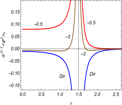
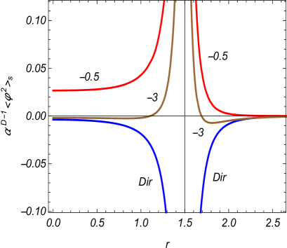
Figure 2: The sphere-induced VEV of the field squared for $D=3$ scalar field as a function of the radial coordinate in the cases of minimally (left panel) and conformally (right panel) coupled fields for Dirichlet boundary condition and for Robin conditions with $\beta=-3,-0.5$. The graphs are plotted for $r_{0}=1.5$, $m\alpha=1$, $t/\alpha=1$.

Figure 3 displays the time-dependence of the sphere-induced contribution in the VEV of the field squared for fixed $r$ (numbers near the curves) and for $r_{0}=1.5$, $m\alpha=1$. The full curves correspond to Dirichlet boundary condition and the dashed curves correspond to Robin boundary condition with $\beta=-0.5$. The graphs for minimal and conformal couplings are presented on the left and right panels, respectively. According to the asymptotic analysis given above, for $D=3$ and in the region $t/\alpha\ll 1$ the boundary-induced VEV of the field squared behaves as $t^{-2}$. In the opposite limit $t/\alpha\gg 1$ the corresponding approximation for minimal coupling (left panel) is obtained from (5.11), according to which $\left\langle\varphi^{2}\right\rangle_{\mathrm{s}}$ behaves as nearly $e^{-(3-\sqrt{5})t/\alpha}$. Contrary to this, in the case of conformal coupling (right panel) the parameter $\nu$ is purely imaginary, $\nu=i\sqrt{3}/2$, and the late time asymptotic is found from (5.16). In this case the field squared decays oscillatory and this behavior is displayed on the right panel as inset for $10^{6}\alpha^{D-1}\left\langle\varphi^{2}\right\rangle_{\mathrm{s}}$.

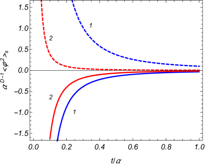
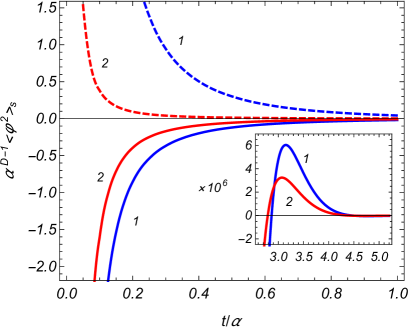
Figure 3: The sphere-induced VEV of the field squared for $D=3$ scalar field as a function of the time coordinate in the cases of minimal (left panel) and conformal (right panel) couplings. The graphs are plotted for $r_{0}=1.5$, $m\alpha=1$ and the numbers near the curves correspond to the values of the radial coordinate. The full and dashed curves present the cases of Dirichlet and Robin (with $\beta=-0.5$) boundary conditions, respectively.

The dependence of the sphere-induced VEV on the coefficient $\beta$ in Robin boundary condition is displayed in Figure 4 for minimally (left panel) and conformally (right panel) coupled fields. The graphs are plotted for $D=3$, $m\alpha=t/\alpha=1$, $r_{0}=1.5$ and the numbers near the curves correspond to the values of the coordinate $r$. The vertical dashed lines correspond to the critical values $\beta_{0}^{\mathrm{(i)}}(u_{0})$ and $\beta_{0}^{\mathrm{(e)}}(u_{0})$ for the Robin coefficient. As seen, depending on the values of the Robin coefficient, the boundary-induced VEV changes the sign. For $\beta\ll-1$ ($\beta=-\infty$ corresponds to Dirichlet boundary condition) $\left\langle\varphi^{2}\right\rangle_{\mathrm{s}}$ is negative and it becomes positive with increasing $\beta$. The VEV increases rapidly when $\beta$ approaches the critical values $\beta_{0}^{(\mathrm{i})}(u_{0})$ and $\beta_{0}^{(\mathrm{e})}(u_{0})$ for the interior and exterior regions, respectively. For $\beta$ near the critical values of $\beta$ the main contribution to the VEV $\left\langle\varphi^{2}\right\rangle_{\mathrm{s}}$ comes from the mode $l=0$.

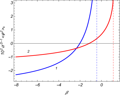
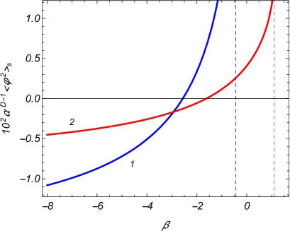
Figure 4: The sphere-induced contribution in the VEV of the field squared for $D=3$ scalar field versus the Robin coefficient in the cases of minimal (left panel) and conformal (right panel) couplings. The graphs are plotted for $m\alpha=t/\alpha=1$, $r_{0}=1.5$ and the numbers near the curves are the values of the coordinate $r$.

6 VEV of the energy-momentum tensor

For the evaluation of the VEV of the energy-momentum tensor we use the formula (2.8). On the base of (4.30) the VEV is decomposed as

$$\left\langle T_{ik}\right\rangle=\left\langle T_{ik}\right\rangle_{0}+\left\langle T_{ik}\right\rangle_{\mathrm{s}},$$ (6.1)

with the boundary-free and sphere-induced contributions $\left\langle T_{ik}\right\rangle_{0}$ and $\left\langle T_{ik}\right\rangle_{\mathrm{s}}$. For points away from the sphere the sphere-induced part is finite and is obtained directly by using the formula that is the analog of (2.8) for sphere-induced contributions. From the symmetry of the problem we expect that the angular stresses are isotropic:

$$\left\langle T_{2}^{2}\right\rangle_{\mathrm{s}}=\left\langle T_{3}^{3}\right\rangle_{\mathrm{s}}=\cdots=\left\langle T_{D}^{D}\right\rangle_{\mathrm{s}}.$$ (6.2)

In addition, we have the trace relation

$$\left\langle T_{k}^{k}\right\rangle_{\mathrm{s}}=\left[D\left(\xi-\xi_{D}\right)\nabla_{k}\nabla^{k}+m^{2}\right]\left\langle\varphi^{2}\right\rangle_{\mathrm{s}}.$$ (6.3)

In the case of a conformally coupled massless field the sphere-induced energy-momentum tensor is traceless. The trace anomaly is contained in the boundary-free part $\left\langle T_{ik}\right\rangle_{0}$.

From the symmetry of the problem we expect that the renormalized VEV $\left\langle T_{ik}\right\rangle_{0}$ is diagonal with isotropic stresses, $\left\langle T_{1}^{1}\right\rangle_{0}=\left\langle T_{2}^{2}\right\rangle_{0}=\cdots=\left\langle T_{D}^{D}\right\rangle_{0}$, and the components $\left\langle T_{i}^{k}\right\rangle_{0}$ are functions of the time coordinate only. The continuity equation $\nabla_{k}\left\langle T_{i}^{k}\right\rangle_{0}=0$ leads to the relation

$$\left\langle T_{1}^{1}\right\rangle_{0}=\frac{\partial_{t/\alpha}\left[\sinh^{D}(t/\alpha)\left\langle T_{0}^{0}\right\rangle_{0}\right]}{D\sinh^{D-1}(t/\alpha)\cosh\left(t/\alpha\right)},$$ (6.4)

between the energy density and stress. For the Bunch-Davies vacuum state one has $\left\langle T_{i}^{k}\right\rangle_{0}^{\mathrm{(BD)}}=\mathrm{const}\cdot\delta_{i}^{k}$. The divergences are determined by the local geometry of the background spacetime and are the same in the unrenormalized VEVs $\left\langle T_{i}^{k}\right\rangle_{0}$ and $\left\langle T_{i}^{k}\right\rangle_{0}^{\mathrm{(BD)}}$ for the hyperbolic and Bunch-Davies vacua. From here it follows that the difference $\Delta\left\langle T_{i}^{k}\right\rangle_{0}=\left\langle T_{i}^{k}\right\rangle_{0}-\left\langle T_{i}^{k}\right\rangle_{0}^{\mathrm{(BD)}}$ needs no renormalization and can be directly evaluated by applying the procedure similar to (2.8) for $G(x,x^{\prime})-G_{\mathrm{BD}}(x,x^{\prime})$, where $G_{\mathrm{BD}}(x,x^{\prime})$ is the Hadamard function for the Bunch-Davies vacuum. In this way, the renormalization of the VEV $\left\langle T_{i}^{k}\right\rangle_{0}$ is reduced to the one for the Bunch-Davies vacuum. The latter procedure has been widely discussed in the literature. For a conformally coupled massless field the tensor $\Delta\left\langle T_{i}^{k}\right\rangle_{0}$ is traceless and from (6.4) it follows that

$$\Delta\left\langle T_{i}^{k}\right\rangle_{0}=\mathrm{const}\frac{\mathrm{diag}\left(1,-1/D,\cdots,-1/D\right)}{\alpha^{D+1}\sinh^{D+1}(t/\alpha)}.$$ (6.5)

A special case of (6.5) for $D=3$, with $\mathrm{const}=-1/(480\pi^{2})$, is considered in [52]. Here, we are mainly interested in the sphere-induced effects and they will be discussed for the interior and exterior regions separately.

6.1 Interior region

By making use of the expression (4.44) for the sphere-induced Hadamard function in (2.8), after long but straightforward calculations, for the diagonal components of the sphere-induced vacuum energy-momentum tensor in the interior region one finds (no summation over $k$)

$$\left\langle T_{k}^{k}\right\rangle_{\mathrm{s}}=-\frac{\sinh^{-2}\left(t/\alpha\right)}{\alpha^{D+1}S_{D}}\sum_{l=0}^{\infty}D_{l}\int_{0}^{\infty}dx\frac{xe^{-i\mu\pi}}{\sin\left(\pi x\right)}\,\frac{\bar{Q}_{x-1/2}^{\mu}\left(u_{0}\right)}{\bar{P}_{x-1/2}^{-\mu}\left(u_{0}\right)}\left[\hat{F}_{k}^{(0)}(y)-\hat{F}_{k}^{(1)}(u)\right]F^{\mathrm{(i)}}\left(x,y,u\right),$$ (6.6)

where the notation

$$F^{\mathrm{(i)}}\left(x,y,u\right)=\frac{P_{\nu-1/2}^{x}\left(y\right)P_{\nu-1/2}^{-x}\left(y\right)}{\left(y^{2}-1\right)^{(D-1)/2}}\frac{[P_{x-1/2}^{-\mu}\left(u\right)]^{2}}{(u^{2}-1)^{D/2-1}}$$ (6.7)

is introduced. The operators $\hat{F}_{0}^{(0)}(y)$ and $\hat{F}_{k}^{(0)}(y)$, $k=1,2,\ldots D$, are defined as

$$\hat{F}_{0}^{(0)}(y) = \left(y^{2}-1\right)\left\{\frac{1}{4}\left(y^{2}-1\right)\partial_{y}^{2}+\left[D\left(\xi+\xi_{D}\right)+\frac{1}{2}\right]y\partial_{y}+m^{2}\alpha^{2}+\xi D^{2}\right\}$$

$$+\frac{\left(D-1\right)^{2}}{4}-x^{2},$$

$$\hat{F}_{k}^{(0)}(y) = \left(y^{2}-1\right)\left\{\left(\xi-\frac{1}{4}\right)\left(y^{2}-1\right)\partial_{y}^{2}+\left[D\left(\xi-\xi_{D}\right)-\frac{1}{2}\right]y\partial_{y}-\xi D\right\}$$ (6.8)

$$+\delta_{1k}\left[x^{2}-\frac{\left(D-1\right)^{2}}{4}\right].$$

The operators $\hat{F}_{k}^{(1)}(u)$ act on the functions of the argument $u$ and are given by the expressions

$$\hat{F}_{0}^{(1)}(u) = \left(\xi-\frac{1}{4}\right)\left[\left(u^{2}-1\right)\partial_{u}^{2}+Du\partial_{u}\right],$$

$$\hat{F}_{1}^{(1)}(u) = \frac{1}{4}\left(u^{2}-1\right)\partial_{u}^{2}+\left[\xi\left(D-1\right)+\frac{D}{4}\right]u\partial_{u}-\frac{l\left(l+n\right)}{u^{2}-1},$$

$$\hat{F}_{k}^{(1)}(u) = \hat{F}_{0}^{(1)}-\xi u\partial_{u}+\frac{1}{D-1}\frac{l\left(l+n\right)}{u^{2}-1},$$ (6.9)

where $k=2,3,\ldots D$. As an additional check for the formula (6.6) we can see that the trace relation (6.3) is obeyed.

The only nonzero off-diagonal component of the vacuum energy-momentum tensor corresponds to $\left\langle T_{0}^{1}\right\rangle_{\mathrm{s}}$ that describes energy flux directed along the radial direction. The corresponding expression reads

$$\left\langle T_{0}^{1}\right\rangle_{\mathrm{s}} = \frac{\sinh^{-3}\left(t/\alpha\right)}{\alpha^{D+2}S_{D}}\sum_{l=0}^{\infty}D_{l}\int_{0}^{\infty}dx\frac{xe^{-i\mu\pi}}{\sin\left(\pi x\right)}\frac{\bar{Q}_{x-1/2}^{\mu}\left(u_{0}\right)}{\bar{P}_{x-1/2}^{-\mu}\left(u_{0}\right)}$$ (6.10)

$$\times\,\left[\left(1/4-\xi\right)\left(y^{2}-1\right)\partial_{y}+\xi y\right]\partial_{r}F^{\mathrm{(i)}}\left(x,y,u\right).$$

With this result, it can be seen that the components given by (6.6) and (6.10) obey the covariant conservation equation $\nabla_{k}\left\langle T_{i}^{k}\right\rangle_{\mathrm{s}}=0$. For the geometry described by (2.1) the latter is reduced to the equations

$$\sum_{k=0,1}\partial_{k}\left\langle T_{0}^{k}\right\rangle_{\mathrm{s}}+\left(D-1\right)\left\langle T_{0}^{1}\right\rangle_{\mathrm{s}}\coth r+\frac{1}{\alpha}\left[\left(D+1\right)\left\langle T_{0}^{0}\right\rangle_{\mathrm{s}}-\left\langle T_{k}^{k}\right\rangle_{\mathrm{s}}\right]\coth\left(t/\alpha\right) = 0,$$

$$\sum_{k=0,1}\partial_{k}\left\langle T_{1}^{k}\right\rangle_{\mathrm{s}}+\frac{D}{\alpha}\left\langle T_{1}^{0}\right\rangle_{\mathrm{s}}\coth\left(t/\alpha\right)+\left(D-1\right)\left(\left\langle T_{1}^{1}\right\rangle_{\mathrm{s}}-\left\langle T_{2}^{2}\right\rangle_{\mathrm{s}}\right)\coth r = 0.$$ (6.11)

The vacuum energy induced by the sphere in volume $V$ is expressed as $E_{\mathrm{(s)}V}=\int_{V}d^{D}x\,\sqrt{|g|}\left\langle T_{0}^{0}\right\rangle_{\mathrm{s}}$. For the spherical layer $r_{1}\leq r\leq r_{2}$ it is presented in the form

$$E_{\mathrm{(s)}V}=\alpha\sinh(t/\alpha)\int_{r_{1}}^{r_{2}}dr\,S_{\mathrm{p}}(r)\left\langle T_{0}^{0}\right\rangle_{\mathrm{s}}.$$

where $S_{\mathrm{p}}(r)=S_{D}\left[\alpha\sinh\left(t/\alpha\right)\sinh r\right]^{D-1}$ is the proper surface area of the sphere with radius $r$. From the first equation (6.11) it follows that

$$\partial_{0}E_{\mathrm{(s)}V}=-\alpha\sinh\left(t/\alpha\right)S_{\mathrm{p}}(r)\left\langle T_{0}^{1}\right\rangle_{\mathrm{s}}|_{r=r_{1}}^{r=r_{2}}+\cosh\left(t/\alpha\right)\int_{r_{1}}^{r_{2}}dr\,S_{\mathrm{p}}(r)\sum_{k=1}^{D}\left\langle T_{k}^{k}\right\rangle_{\mathrm{s}}.$$ (6.12)

This relation shows that the quantity

$$\left\langle\tilde{T}_{0}^{1}\right\rangle_{\mathrm{s}}=\alpha\sinh\left(t/\alpha\right)\left\langle T_{0}^{1}\right\rangle_{\mathrm{s}}$$ (6.13)

is the energy flux density per unit proper surface area. The latter can be written as $\left\langle\tilde{T}_{0}^{1}\right\rangle_{\mathrm{s}}=n_{k}\left\langle T_{0}^{k}\right\rangle_{\mathrm{s}}$, where $n_{k}$ is the unit spatial vector normal to the sphere (external with respect to the volume $V$). For the spherical layer corresponding to (6.12) one has $n_{k}=\pm\delta_{k}^{1}\alpha\sinh\left(t/\alpha\right)$, where the upper and lower signs stand for the spheres $r=r_{2}$ and $r=r_{1}$, respectively.

Let us consider some limiting cases of the general result for the sphere-induced VEV of the energy-momentum tensor. In the flat spacetime limit $\alpha\rightarrow\infty$, by using the relation (4.31) for the product of the associated Legendre functions, it can be seen that from (6.6) and (6.10) the boundary-induced VEV for the conformal vacuum inside a sphere in background of the Milne universe is obtained (see [48]).

Another special case corresponds to a conformally coupled massless scalar field. In this case one has $\nu=1/2$ and the function (6.7) is simplified to

$$F^{\mathrm{(i)}}\left(x,y,u\right)=\frac{\sin\left(\pi x\right)/(\pi x)}{(y^{2}-1)^{(D-1)/2}}\frac{[P_{x-1/2}^{-\mu}\left(u\right)]^{2}}{(u^{2}-1)^{D/2-1}}.$$ (6.14)

With this function, the off-diagonal component (6.10) vanishes for $\xi=\xi_{D}$. For the diagonal components we find (no summation over $k$)

$$\left\langle T_{k}^{k}\right\rangle_{\mathrm{s}}=\frac{\left\langle T_{k}^{k}\right\rangle_{\mathrm{s}}^{\mathrm{(st)}}}{\sinh^{D+1}(t/\alpha)},$$ (6.15)

where

$$\left\langle T_{k}^{k}\right\rangle_{\mathrm{s}}^{\mathrm{(st)}}=\sum_{l=0}^{\infty}\frac{e^{-i\mu\pi}D_{l}}{\pi\alpha^{D+1}S_{D}}\int_{0}^{\infty}dx\,\frac{\bar{Q}_{x-1/2}^{\mu}\left(u_{0}\right)}{\bar{P}_{x-1/2}^{-\mu}\left(u_{0}\right)}\hat{F}_{k}^{\mathrm{(st)}}(u)\frac{[P_{x-1/2}^{-\mu}\left(u\right)]^{2}}{(u^{2}-1)^{D/2-1}}.$$ (6.16)

with the operators

$$\hat{F}_{0}^{\mathrm{(st)}}(u) = -\frac{u^{2}-1}{4D}\partial_{u}^{2}-\frac{u}{4}\partial_{u}+x^{2},$$

$$\hat{F}_{1}^{\mathrm{(st)}}(u) = \frac{u^{2}-1}{4}\partial_{u}^{2}+\frac{D^{2}-D+1/2}{2D}u\partial_{u}+\frac{\left(D-1\right)^{3}}{4D}-\frac{l\left(l+n\right)}{u^{2}-1}-x^{2},$$

$$\hat{F}_{2}^{\mathrm{(st)}}(u) = -\frac{u^{2}-1}{4D}\partial_{u}^{2}-\frac{2D-1}{4D}u\partial_{u}-\frac{\left(D-1\right)^{2}}{4D}+\frac{l}{D-1}\frac{l+n}{u^{2}-1}.$$ (6.17)

The quantity (6.16) is the boundary-induced VEV of the energy-momentum tensor for a conformally coupled massless scalar field inside a sphere with radius $r_{0}$ in background of a static negative constant curvature space with the curvature radius $\alpha$. It is obtained from the more general result in [49] in the special case $m=0$ and $\xi=\xi_{D}$ (see also [48]).

Let us consider the asymptotics with respect to the ratio $t/\alpha$. At the early stages of the expansion, corresponding to $t/\alpha\ll 1$, by using the relation (5.8) we find (no summation over $k$)

$$\left\langle T_{k}^{k}\right\rangle_{\mathrm{s}}\approx\sum_{l=0}^{\infty}\frac{e^{-i\mu\pi}D_{l}}{\pi S_{D}t^{D+1}}\int_{0}^{\infty}dx\,\frac{\bar{Q}_{x-1/2}^{\mu}\left(u_{0}\right)}{\bar{P}_{x-1/2}^{-\mu}\left(u_{0}\right)}\hat{R}_{k}(u)\frac{[P_{x-1/2}^{-\mu}\left(u\right)]^{2}}{(u^{2}-1)^{D/2-1}},$$ (6.18)

where the operators $\hat{R}_{k}(u)$ are defined by

$$\hat{R}_{0}(u) = \left(\xi-\frac{1}{4}\right)\left[\left(u^{2}-1\right)\partial_{u}^{2}+Du\partial_{u}\right]+x^{2}+D\left(D-1\right)\left(\xi-\xi_{D}\right),$$

$$\hat{R}_{1}(u) = \frac{1}{4}\left(u^{2}-1\right)\partial_{u}^{2}+\left[\left(D-1\right)\xi+\frac{D}{4}\right]u\partial_{u}-\frac{l\left(l+n\right)}{u^{2}-1}-x^{2}-\frac{D-1}{4}\left(4\xi-D+1\right),$$

$$\hat{R}_{2}(u) = \left(\xi-\frac{1}{4}\right)\left(u^{2}-1\right)\partial_{u}^{2}+\left[\left(D-1\right)\xi-\frac{D}{4}\right]u\partial_{u}+\frac{l}{D-1}\frac{l+n}{u^{2}-1}-\xi\left(D-1\right).$$ (6.19)

We note that the sphere-induced VEV of the energy-momentum tensor for a scalar field in the static spacetime with negative constant curvature spatial sections is expressed in terms of the operators (6.19) as (see [49], no summation over $k$)

$$\langle T_{i}^{k}\rangle_{\mathrm{s}}^{\mathrm{(st)}}=\delta_{i}^{k}\sum_{l=0}^{\infty}\frac{e^{-i\mu\pi}D_{l}}{\pi S_{D}\alpha^{D+1}}\int_{x_{m}}^{\infty}dx\,x\frac{\bar{Q}_{x-1/2}^{\mu}(u_{0})}{\bar{P}_{x-1/2}^{-\mu}(u_{0})}\frac{\hat{R}_{k}(u)-m^{2}a^{2}\delta_{k}^{0}}{\sqrt{x^{2}-x_{m}^{2}}}\frac{P_{x-1/2}^{-\mu}(u)}{(u^{2}-1)^{D/2-1}},$$ (6.20)

where $x_{m}=\sqrt{m^{2}\alpha^{2}-D(D-1)\left(\xi-\xi_{D}\right)}$. For $\xi=\xi_{D}$ the operators (6.19) are reduced to the ones in (6.17): $\hat{R}_{k}(u)=\hat{F}_{k}^{\mathrm{(st)}}(u)$. In the same limit, $t/\alpha\ll 1$, for the off-diagonal component we get

$$\left\langle T_{0}^{1}\right\rangle_{\mathrm{s}}\approx D\left(\xi-\xi_{D}\right)\sum_{l=0}^{\infty}\frac{e^{-i\mu\pi}D_{l}}{\pi S_{D}t^{D+2}}\int_{0}^{\infty}dx\,\frac{\bar{Q}_{x-1/2}^{\mu}\left(u_{0}\right)}{\bar{P}_{x-1/2}^{-\mu}\left(u_{0}\right)}\partial_{r}\frac{[P_{x-1/2}^{-\mu}\left(u\right)]^{2}}{(u^{2}-1)^{D/2-1}}.$$ (6.21)

The energy flux density per unit proper surface area is given as $\left\langle\tilde{T}_{0}^{1}\right\rangle_{\mathrm{s}}\approx t\left\langle T_{0}^{1}\right\rangle_{\mathrm{s}}$ and for non-conformally coupled fields it is of the same order as the diagonal components. The expressions in the right-hand sides of (6.18) and (6.21) coincide with the leading terms in the expansions of the corresponding VEVs for a sphere in the Milne universe at early stages $mt\ll 1$. This is related to the fact that the effects of curvature of dS spacetime are weak in the range $t/\alpha\ll 1$.

At late stages of the expansion, $t/\alpha\gg 1$, we use the asymptotic (5.10). In the case $\nu>0$, to the leading order, for the diagonal components we get (no summation over $k$)

$$\left\langle T_{k}^{k}\right\rangle_{\mathrm{s}}\approx\frac{a_{k}}{\alpha^{2}}\left\langle\varphi^{2}\right\rangle_{\mathrm{s}}\,,$$ (6.22)

where the VEV of the field squared is estimated as (5.11) and

$$a_{0} = \frac{D}{4}\left[D-2\nu-4\xi\left(D+1-2\nu\right)\right],$$

$$a_{1} = a_{2}=\frac{2\nu}{D}a_{0}.$$ (6.23)

In this limit the sphere-induced VEV is suppressed by the factor $e^{-\left(D-2\nu\right)t/\alpha}$. The corresponding asymptotic for the off-diagonal component has the form

$$\left\langle T_{0}^{1}\right\rangle_{\mathrm{s}}\approx\frac{4a_{0}}{D\alpha^{3}}e^{-2t/\alpha}\partial_{r}\left\langle\varphi^{2}\right\rangle_{\mathrm{s}},$$ (6.24)

and the suppression is stronger, by the factor $e^{-\left(D+2-2\nu\right)t/\alpha}$. Note that at late stages of the expansion we have the relation

$$\left\langle\tilde{T}_{0}^{1}\right\rangle_{\mathrm{s}}=\frac{2}{D}e^{-t/\alpha}\partial_{r}\left\langle T_{0}^{0}\right\rangle_{\mathrm{s}},$$ (6.25)

between the energy and the energy flux densities. The asymptotics (6.22) and (6.24) are also valid for $\nu=0$ but now the behavior of $\left\langle\varphi^{2}\right\rangle_{\mathrm{s}}$ is described by (5.13). Note that in this case the leading terms in the vacuum stresses vanish and we have (no summation over $k$) $|\left\langle T_{k}^{k}\right\rangle_{\mathrm{s}}|\ll|\left\langle T_{0}^{0}\right\rangle_{\mathrm{s}}|$, where $k=1,2,\ldots,D$.

For $t/\alpha\gg 1$ and purely imaginary $\nu$, $\nu=i|\nu|$, we use the asymptotic formula (5.15). To the leading order this gives

$$\left\langle T_{0}^{0}\right\rangle_{\mathrm{s}} \approx m^{2}\left\langle\varphi^{2}\right\rangle_{\mathrm{s}}+\frac{2^{D}|\nu|e^{-Dt/\alpha}}{\pi S_{D}\alpha^{D+1}}\overset{\infty}{\sum_{l=0}}D_{l}\int_{0}^{\infty}dx\frac{xe^{-i\mu\pi}}{\sin\left(\pi x\right)}\,\frac{\bar{Q}_{x-1/2}^{\mu}\left(u_{0}\right)}{\bar{P}_{x-1/2}^{-\mu}\left(u_{0}\right)}$$ (6.26)

$$\times\frac{[P_{x-1/2}^{-\mu}\left(u\right)]^{2}}{\sinh^{D-2}r}B_{\nu}(x)\left\{2D\left(\xi-\frac{1}{4}\right)\sin\left[\phi(t,x)\right]+|\nu|\cos\left[\phi(t,x)\right]\right\},$$

for the energy density and

$$\left\langle T_{k}^{k}\right\rangle_{\mathrm{s}} \approx -\frac{2^{D}|\nu|e^{-Dt/\alpha}}{\pi S_{D}\alpha^{D+1}}\sum_{l=0}^{\infty}D_{l}\int_{0}^{\infty}dx\frac{xe^{-i\mu\pi}}{\sin\left(\pi x\right)}\,\frac{\bar{Q}_{x-1/2}^{\mu}\left(u_{0}\right)}{\bar{P}_{x-1/2}^{-\mu}\left(u_{0}\right)}\frac{[P_{x-1/2}^{-\mu}\left(u\right)]^{2}}{\sinh^{D-2}r}B_{\nu}(x)$$ (6.27)

$$\times\left\{\left(1-4\xi\right)|\nu|\cos\left[\phi(t,x)\right]+2\left[\left(D+1\right)\xi-\frac{D}{4}\right]\sin\left[\phi(t,x)\right]\right\},$$

for the stresses (no summation over $k$) $k=1,2,\ldots,D$. Here, the phase $\phi(t,x)$ is defined in (5.17). The asymptotic expression for the energy flux density takes the form

$$\left\langle\tilde{T}_{0}^{1}\right\rangle_{\mathrm{s}} \approx \frac{D-4\left(D+1\right)\xi}{2\alpha^{2}e^{t/\alpha}}\partial_{r}\left\langle\varphi^{2}\right\rangle_{\mathrm{s}}+\frac{2^{D}|\nu|\left(4\xi-1\right)}{\pi\alpha^{D+1}S_{D}e^{(D+1)t/\alpha}}\sum_{l=0}^{\infty}D_{l}\int_{0}^{\infty}dx\frac{xe^{-i\mu\pi}}{\sin\left(\pi x\right)}$$ (6.28)

$$\times\,\frac{\bar{Q}_{x-1/2}^{\mu}\left(u_{0}\right)}{\bar{P}_{x-1/2}^{-\mu}\left(u_{0}\right)}\partial_{r}\frac{[P_{x-1/2}^{-\mu}\left(u\right)]^{2}}{\sinh^{D-2}r}B_{\nu}(x)\sin\left[\phi(t,x)\right].$$

The expression for $\left\langle\varphi^{2}\right\rangle_{\mathrm{s}}$ in (6.26) and (6.28) is given by (5.16) and $B_{\nu}(x)$, $\phi_{\nu}(x)$ are defined by (5.18). For purely imaginary $\nu$ the decay of the vacuum energy-momentum tensor at late stages is damping oscillatory.

Now we turn to the asymptotics with respect to the radial coordinate. Near the center the dominant contributions come from the terms with $l=0,1$ and to the leading order we get (no summation over $k$)

$$\left\langle T_{k}^{k}\right\rangle_{\mathrm{s}}\approx\frac{2\sinh^{-2}\left(t/\alpha\right)}{\left(4\pi\right)^{D/2}\alpha^{D+1}\Gamma\left(D/2\right)}\int_{0}^{\infty}dx\sum_{l=0,1}\frac{xe^{-i\mu\pi}}{\sin\left(\pi x\right)}\frac{\bar{Q}_{x-1/2}^{\mu}\left(u_{0}\right)}{\bar{P}_{x-1/2}^{-\mu}\left(u_{0}\right)}\hat{F}_{\left(k\right)l}\frac{P_{\nu-1/2}^{x}\left(y\right)P_{\nu-1/2}^{-x}\left(y\right)}{(y^{2}-1)^{(D-1)/2}},$$ (6.29)

where $\hat{F}_{\left(k\right)0}=\hat{F}_{k}^{(0)}(y)$, with the operators from (6.8), and

$$\hat{F}_{\left(0\right)1} = 2\xi-\frac{1}{2},$$

$$\hat{F}_{\left(1\right)1} = \hat{F}_{\left(2\right)1}=\frac{2}{D}\left[\left(D-1\right)\xi-\frac{D-2}{4}\right].$$ (6.30)

The dominant contribution to the off-diagonal component comes from $l=1$ term and one finds

$$\left\langle T_{0}^{1}\right\rangle_{\mathrm{s}} \approx \frac{e^{-i\pi D/2}r\sinh^{-3}\left(t/\alpha\right)}{\left(4\pi\right)^{D/2}\alpha^{D+2}D\Gamma\left(D/2\right)}\int_{0}^{\infty}dx\frac{x}{\sin\left(\pi x\right)}\,\frac{\bar{Q}_{x-1/2}^{D/2}\left(u_{0}\right)}{\bar{P}_{x-1/2}^{-D/2}\left(u_{0}\right)}$$ (6.31)

$$\times\left[\left(1-4\xi\right)\left(y^{2}-1\right)\partial_{y}+4\xi y\right]\frac{P_{\nu-1/2}^{x}\left(y\right)P_{\nu-1/2}^{-x}\left(y\right)}{(y^{2}-1)^{(D-1)/2}},$$

and it linearly vanishes at the sphere center.

For points near the sphere the main contribution to the integral and series in (6.6) comes from large $l$ and $x$. By using the large $x$ asymptotic (5.23) we see that the dependence on $y$ in the function (6.7) appears in the form $(y^{2}-1)^{(1-D)/2}$ and the derivatives in (6.8) with respect to $y$ are easily evaluated. Keeping the leading terms in $x$ we can see that for the components $\left\langle T_{k}^{k}\right\rangle_{\mathrm{s}}$, $k=0,2,\ldots,D$, the leading terms in the asymptotic expansions over the distance from the sphere are expressed in terms of the corresponding components $\left\langle T_{k}^{k}\right\rangle_{\mathrm{s}}^{\mathrm{(st)}}$ for a sphere in static spacetime with negative constant curvature space as $\left\langle T_{k}^{k}\right\rangle_{\mathrm{s}}\approx\left\langle T_{k}^{k}\right\rangle_{\mathrm{s}}^{\mathrm{(st)}}/\sinh^{D+1}\left(t/\alpha\right)$. By using the asymptotics for $\left\langle T_{k}^{k}\right\rangle_{\mathrm{s}}^{\mathrm{(st)}}$ from [49] we find (no summation over $k$)

$$\left\langle T_{k}^{k}\right\rangle_{\mathrm{s}}\approx\frac{(2\delta_{0B}-1)D\Gamma((D+1)/2)\left(\xi-\xi_{D}\right)}{2^{D}\pi^{(D+1)/2}\left[\alpha\sinh(t/\alpha)(r_{0}-r)\right]^{D+1}},$$ (6.32)

for $k=0,2,\ldots,D$. In order to find the asymptotics for the radial stress and the off-diagonal component it is more convenient to use the covariant conservation equations (6.11). From the first equation it follows that

$$\left\langle T_{0}^{1}\right\rangle_{\mathrm{s}}\approx\frac{1}{\alpha}\coth\left(t/\alpha\right)\left(r_{0}-r\right)\left\langle T_{0}^{0}\right\rangle_{\mathrm{s}}.$$ (6.33)

With this result, from the second equation in (6.11) we get

$$\left\langle T_{1}^{1}\right\rangle_{\mathrm{s}}\approx\frac{D-1}{D}\coth\left(r_{0}\right)\left(r_{0}-r\right)\left\langle T_{0}^{0}\right\rangle_{\mathrm{s}}.$$ (6.34)

The leading terms do not depend on the mass. For a conformally coupled field they vanish and one needs to keep the next-to-leading order terms. Note that the leading terms in the VEVs of the field squared and of the diagonal components, given by (5.25) and (6.32), are obtained from the corresponding terms for a sphere in the Minkowski bulk (see [53]) replacing the distance from the sphere by the proper distance $\alpha\sinh(t/\alpha)(r_{0}-r)$ for the geometry at hand.

6.2 Exterior region

The VEV of the energy-momentum tensor outside the sphere is decomposed as (6.1), where the sphere-induced contribution is obtained from (2.8) and (4.29). The expression for the diagonal components reads (no summation over $k$):

$$\left\langle T_{k}^{k}\right\rangle_{\mathrm{s}}=-\frac{\sinh^{-2}\left(t/\alpha\right)}{\alpha^{D+1}S_{D}}\sum_{l=0}^{\infty}D_{l}\int_{0}^{\infty}dx\frac{e^{-i\mu\pi}x}{\sin\left(\pi x\right)}\frac{\bar{P}_{x-1/2}^{-\mu}\left(u_{0}\right)}{\bar{Q}_{x-1/2}^{\mu}\left(u_{0}\right)}\,\left[\hat{F}_{k}^{(0)}(y)-\hat{F}_{k}^{(1)}(u)\right]F^{\mathrm{(e)}}\left(x,y,u\right),$$ (6.35)

with the function

$$F^{\mathrm{(e)}}\left(x,y,u\right)=\frac{P_{\nu-1/2}^{x}\left(y\right)P_{\nu-1/2}^{-x}\left(y\right)}{\sinh^{D-1}\left(t/\alpha\right)}\frac{[Q_{x-1/2}^{\mu}\left(u\right)]^{2}}{\sinh^{D-2}r},$$ (6.36)

and the operators $\hat{F}_{k}^{(0)}(y)$ and $\hat{F}_{k}^{(1)}(u)$ are defined by (6.8) and (6.9). The nonzero off-diagonal component is expressed as

$$\left\langle T_{0}^{1}\right\rangle_{\mathrm{s}} = \frac{\sinh^{-3}\left(t/\alpha\right)}{\alpha^{D+2}S_{D}}\sum_{l=0}^{\infty}D_{l}\int_{0}^{\infty}dx\frac{xe^{-i\mu\pi}}{\sin\left(\pi x\right)}\,\frac{\bar{P}_{x-1/2}^{-\mu}\left(u_{0}\right)}{\bar{Q}_{x-1/2}^{\mu}\left(u_{0}\right)}$$ (6.37)

$$\times\left[\left(1/4-\xi\right)\left(y^{2}-1\right)\partial_{y}+\xi y\right]\partial_{r}F^{\mathrm{(e)}}\left(x,y,u\right).$$

Recall that the energy flux density per unit proper surface area is given by (6.13). One can check that the components (6.35) and (6.37) obey the trace relation (6.3) and covariant conservation equations (6.11).

For a conformally coupled massless field the off-diagonal component is zero and for the diagonal components we have the relation (6.15), where the VEV outside a sphere in static spacetime with a constant negative curvature space is given by [49]

$$\left\langle T_{i}^{k}\right\rangle_{\mathrm{s}}^{\mathrm{(st)}}=\delta_{i}^{k}\sum_{l=0}^{\infty}\frac{e^{-i\mu\pi}D_{l}}{\pi\alpha^{D+1}S_{D}}\int_{0}^{\infty}dx\,\frac{\bar{P}_{x-1/2}^{-\mu}\left(u_{0}\right)}{\bar{Q}_{x-1/2}^{\mu}\left(u_{0}\right)}\hat{F}_{k}^{\mathrm{(st)}}\frac{[Q_{x-1/2}^{\mu}\left(u\right)]^{2}}{(u^{2}-1)^{D/2-1}},$$ (6.38)

with the operators $\hat{F}_{k}^{\mathrm{(st)}}$ defined in (6.17). In the limit $\alpha\rightarrow\infty$ and for the case of a massive field with general curvature coupling parameter, from (6.35) and (6.37) we obtain the corresponding VEVs for the conformal vacuum outside a spherical boundary in the Milne universe.

At early stages of the expansion, $t/\alpha\ll 1$, the leading terms of the asymptotic expansion of the sphere-induced VEV $\left\langle T_{i}^{k}\right\rangle_{\mathrm{s}}$ in the exterior region are obtained from (6.18) and (6.21) by the replacements (4.46). For a conformally coupled scalar field, to the leading order, we have the relation $\left\langle T_{i}^{k}\right\rangle_{\mathrm{s}}\approx\left(\alpha/t\right)^{D+1}\left\langle T_{i}^{k}\right\rangle_{\mathrm{s}}^{\mathrm{(st)}}$, with $\left\langle T_{i}^{k}\right\rangle_{\mathrm{s}}^{\mathrm{(st)}}$ given by (6.38). At late stages, $t/\alpha\gg 1$, and for $\nu\geq 0$, the asymptotic expressions for the components of the energy-momentum tensor are related to the corresponding asymptotic for the VEV of the field squared by the formulas (6.22) and (6.24). For purely imaginary $\nu$, the behavior of the sphere-induced parts in the VEV of the energy-momentum tensor is described by the formulas (6.26)-(6.28) with the replacements (4.46). In this limit, to the leading order, the stresses are isotropic.

For points near the sphere the leading terms in the asymptotic expansions of the energy density and stresses $\left\langle T_{k}^{k}\right\rangle_{\mathrm{s}}$, $k=0,2,\ldots,D$, are given by (6.32) with the replacement $r_{0}-r\rightarrow r-r_{0}$. For points near the sphere these components have the same sign in the interior and exterior regions. The relations (6.33) and (6.34) for the off-diagonal component and the radial stress remain the same and, hence, near the sphere these components have opposite signs outside and inside the sphere. For large distances from sphere the diagonal components of sphere-induced VEV of energy-momentum tensor and the energy flux density are approximately given by (no summation over $k$)

$$\left\langle T_{k}^{k}\right\rangle_{\mathrm{s}} \approx \frac{\hat{G}_{k}(y)\left\langle\varphi^{2}\right\rangle_{\mathrm{s}}}{\alpha^{2}\sinh^{2}\left(t/\alpha\right)},\text{ }k=0,1,\ldots,D,$$

$$\left\langle T_{0}^{1}\right\rangle_{\mathrm{s}} \approx \frac{D-1}{\alpha^{3}\sinh^{3}\left(t/\alpha\right)}\left[\left(1/4-\xi\right)\left(y^{2}-1\right)\partial_{y}+\xi y\right]\left\langle\varphi^{2}\right\rangle_{\mathrm{s}},$$ (6.39)

where $\left\langle\varphi^{2}\right\rangle_{\mathrm{s}}$ is described by the asymptotic expression (5.28). The operators in (6.39) are defined as

$$\hat{G}_{0}(y) = \hat{F}_{0}^{(0)}(y)|_{x=0},\;\hat{G}_{1}(y)=\hat{F}_{2}^{(0)}(y)|_{x=0}+\left(D-1\right)^{2}\left(\xi-1/4\right),$$

$$\;\hat{G}_{k}(y) = \hat{F}_{2}^{(0)}(y)|_{x=0}-\left(D-1\right)\xi,\;k=2,\ldots,D.$$ (6.40)

Hence, at large distances from the sphere we have an exponential suppression of the sphere-induced VEVs by the factor $e^{-(D-1)r}/r$. For a conformally coupled massless field the leading terms vanish. The corresponding behavior is obtained by using the conformal relation (6.15) and the results from [49] for static background. In this special case the energy flux vanishes and the decay of the sphere-induced VEVs in the diagonal components is stronger, like $e^{-(D-1)r}/r^{2}$.

6.3 Numerical results

As before, the numerical results for the sphere-induced energy density and energy flux will be presented for $D=3$ minimally and conformally coupled scalar fields. In Figure 5, the boundary-induced energy (left panel) and energy flux (right panel) densities are displayed as functions of the radial coordinate for a minimally coupled scalar field. The graphs are plotted for $m\alpha=t/\alpha=1$, $r_{0}=1.5$ in the cases of Dirichlet boundary condition and for Robin conditions with $\beta=-3,-0.5$ (the numbers near the curves). The same graphs for a conformally coupled scalar field are presented in Figure 6. For both minimally and conformally coupled fields, the energy flux in the interior and exterior egions is directed from the boundary for Dirichlet boundary condition and towards the boundary for Robin conditions.

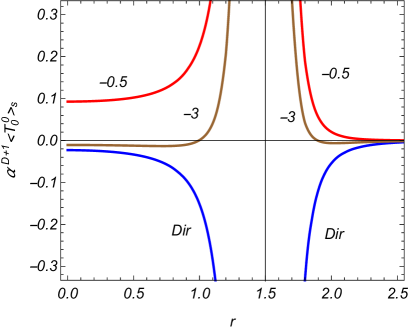
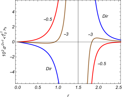
Figure 5: The sphere-induced energy density and the flux density as functions of the radial coordinate for $D=3$ minimally coupled scalar field with Dirichlet and Robin boundary conditions ($\beta=-3,-0.5$). The graphs are plotted for $m\alpha=t/\alpha=1$, $r_{0}=1.5$.

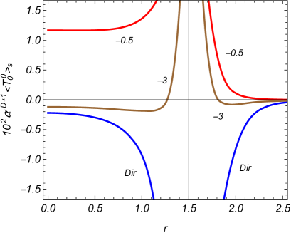
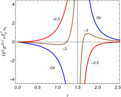
Figure 6: The same as in Figure 5 for a conformally coupled field.

The leading term for the energy density in the expansion near the sphere center is given by (6.29). The energy flux linearly vanishes at the center as a function of the radial coordinate (see (6.31)). For a minimally coupled field the leading term in the asymptotic expansion of the energy density near the sphere is given by (6.32) and the sphere-induced VEV behaves as $(r-r_{0})^{-4}$. Near the sphere it has the same sign for the interior and exterior regions. The leading term for the energy flux is obtained from (6.33) and it has opposite signs inside and outside the sphere. The corresponding divergence on the sphere is weaker, like $(r-r_{0})^{-3}$. The same is the case for the radial stress (see (6.34)). For a conformally coupled field the leading terms in the near-sphere expansions vanish and the energy density and energy flux diverge as $(r-r_{0})^{-3}$ and $(r-r_{0})^{-2}$, respectively. At large distances from the sphere, the boundary-induced contributions in both the energy density and energy flux are suppressed by the factor $e^{-2r}$.

Figure 7 displays the time-dependence of the sphere-induced VEVs in the energy density (left panel) and energy flux (right panel) for a minimally coupled scalar field. The graphs are plotted for $r_{0}=1.5$, $m\alpha=1$ and the numbers near the curves are the values of the radial coordinate $r$. The full curves correspond to Dirichlet boundary condition and the dashed curves correspond to Robin boundary condition with $\beta=-0.5$. The same graphs for a conformally coupled field are depicted in Figure 8. According to (6.18), the boundary-induced contribution in the energy density is nearly proportional to $1/t^{4}$ for $t/\alpha\ll 1$. For the energy flux density and for a minimally coupled field one has the behavior $\left\langle\tilde{T}_{0}^{1}\right\rangle_{\mathrm{s}}\propto 1/t^{4}$. For a conformally coupled field the leading term in the corresponding asymptotic expansion vanishes and $|\left\langle\tilde{T}_{0}^{1}\right\rangle_{\mathrm{s}}|\ll|\left\langle T_{0}^{0}\right\rangle_{\mathrm{s}}|$ in the range $t/\alpha\ll 1$. This is seen from Figure 8. In the opposite limit, $t/\alpha\gg 1$, the corresponding approximation for minimal coupling is obtained from (6.22), according to which $\left\langle T_{0}^{0}\right\rangle_{\mathrm{s}}$, as a function of $t$, behaves similar to the sphere-induced VEV of the field squared. The corresponding approximation for a conformally coupled scalar field is given by (6.26). The oscillatory damping of the sphere-induced VEVs in the case of a conformally coupled field is separately displayed as insets (for $10^{7}\alpha^{D+1}\left\langle T_{0}^{0}\right\rangle_{\mathrm{s}}$ and $10^{8}\alpha^{D+1}\left\langle\tilde{T}_{0}^{1}\right\rangle_{\mathrm{s}}$).

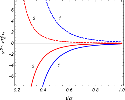
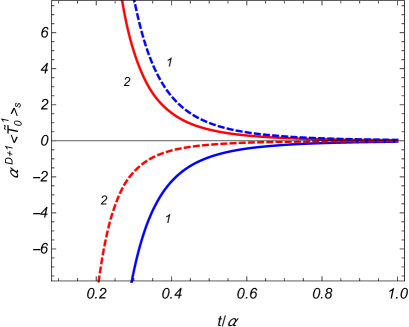
Figure 7: The sphere-induced energy density (left panel) and the energy flux (right panel) for a minimally coupled field versus the time coordinate at fixed values of the radial coordinate (the numbers near the curves). For the sphere radius we have taken $r_{0}=1.5$ and for the field mass $m\alpha=1$.

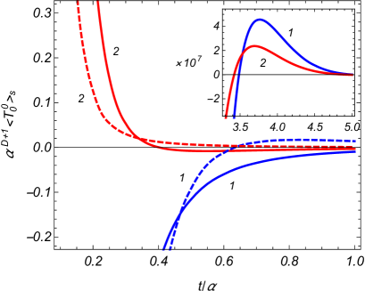
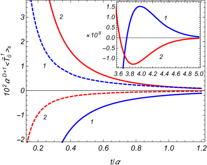
Figure 8: The same as in Figure 7 for a conformally coupled scalar field.

Figure 9 presents the dependence of the sphere-induced VEV in the energy density (left panel) and energy flux (right panel) on the coefficient $\beta$ in Robin boundary condition for a minimally coupled scalar fields. The graphs are plotted for $D=3$, $m\alpha=t/\alpha=1$, $r_{0}=1.5$. The numbers near the curves represent the values of the radial coordinate $r$. For the interior region we have taken $r=1$ and for the exterior region $r=2$. The vertical dashed lines correspond to the critical values of the Robin coefficient in the interior and exterior regions. The same graphs for a conformally coupled field are presented in Figure 10. For the values of the parameter $\beta$ close to the critical values the sphere-induced energy density is positive. For large values of $-\beta$, the VEVs tend to the values corresponding to Dirichlet boundary condition and the energy density is negative. For some intermediate value of $\beta$ the sphere-induced contribution vanishes.

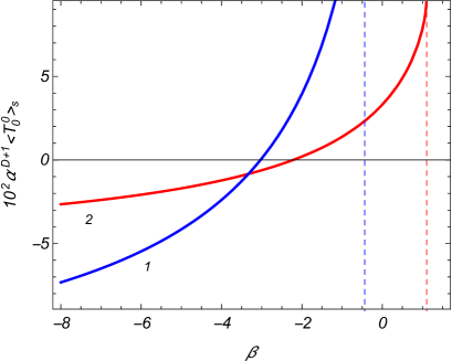
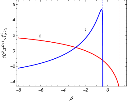
Figure 9: The boundary-induced energy density (left panel) and energy flux (right panel) for $D=3$ minimally coupled scalar field as functions of the coefficient $\beta$ in Robin boundary condition. The graphs are plotted for $m\alpha=1$, $t/\alpha=1$, $r_{0}=1.5$ and the numbers near the curves correspond to the values of $r$.

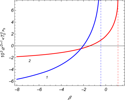
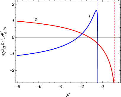
Figure 10: The same as in Figure 9 for a conformally coupled field.

7 Conclusion

For a given spacetime geometry, the quantum field theoretical vacuum is an observer dependent notion. Among the interesting directions in the investigations of the Casimir effect is the dependence of the physical characteristics on the choice of the vacuum state. The previous studies of the boundary and topology induced effects in dS spacetime mainly consider the dS invariant Bunch-Davies vacuum state. The present paper concerns the boundary induced effects on the local VEVs of a scalar field with general curvature coupling for the hyperbolic vacuum in dS spacetime. As a boundary we have considered a spherical shell with a constant comoving radius in hyperbolic spatial coordinates. In inflationary coordinates this corresponds to a spherical shell with time dependent radius, given by (2.6). Note that the Casimir effect for a spherical boundary with constant comoving radius in inflationary coordinates and for the Bunch-Davies vacuum state has been investigated in [26].

As the first step in the investigation of the local VEVs we have constructed the complete set of mode functions in hyperbolic coordinates without specifying the vacuum state. Then, the mode functions are specified for the conformal (hyperbolic) vacuum. It has been shown that the latter coincides with the adiabatic vacuum. By using the complete set of mode functions, the Hadamard functions are evaluated in the boundary-free geometry, outside the spherical shell and inside the shell. For both regions in the problem with a sphere, the contributions in the Hadamard function induced by the boundary are separated explicitly. Inside the sphere, the eigenvalues of the quantum number $z$ are given implicitly, as roots of the equation (4.33), and for the extraction of the sphere-induced part we have used the summation formula (4.42). The corresponding contribution in the Hadamard function is given by (4.44) and the explicit knowledge of the eigenvalues for $z$ is not required. Similar representations can be obtained for other two-point functions (for example, for the Wightman function).

As a local characteristic of the hyperbolic vacuum, the VEV of the field squared is considered. The latter is obtained taking the coincidence limit of the arguments in the Hadamard function. In that limit divergences arise and a renormalization is required. Having the decomposed representation of the Hadamard function, for points away from the sphere the renormalization is reduced to the one in the boundary-free geometry. The VEVs of the field squared inside and outside the sphere are expressed as (5.3) and (5.26). The corresponding expressions for the VEVs of the diagonal components of the energy-momentum tensor are given by the expressions (6.6) and (6.35). Note that the expressions for the interior and exterior regions are obtained from each other by the replacements (4.46). An interesting feature in the problem under consideration is the presence of the vacuum energy flux along the radial direction. The latter is described by the off-diagonal component of the energy-momentum tensor, given by (6.10) and (6.37). Depending on the value of the Robin coefficient and also on the radial coordinate, that component may change the sign. This shows that the energy flux can be directed either from the sphere or towards the sphere.

The general formulas for the VEVs are complicated and in order to clarify the qualitative features we have considered limiting cases and various asymptotic regions of the parameters. In the flat spacetime limit, corresponding to $\alpha\rightarrow\infty$, the line element (2.1) is reduced to the line element (3.9) for the Milne universe. It is checked that, in this limit, from the results given above the corresponding VEVs are obtained for a sphere in the Milne universe (see [48]), assuming that the scalar field is prepared in the conformal vacuum. For a conformally coupled massless scalar field the problem under consideration is conformally related to the problem with a spherical boundary in static spacetime with constant negative curvature space. As another check, we have shown that the VEVs in those problems are connected by the standard conformal relation. Note that in this special case the energy flux vanishes.

In early stages of the expansion, corresponding to $t/\alpha\ll 1$, the effects of the spacetime curvature on the sphere-induced VEVs are weak and, to the leading order, they coincide with the corresponding VEVs for a sphere in the Milne universe. The effects of gravity are essential for $t/\alpha\gtrsim 1$. In particular, at late stages, $t/\alpha\gg 1$, the behavior of the VEVs is qualitatively different for positive and purely imaginary values of the parameter $\nu$ in (2.15). For $\nu>0$ the decay of the sphere-induced VEVs, as functions of the time coordinate, is monotonic, as $e^{-\left(D-2\nu\right)t/\alpha}$ for $\left\langle\varphi^{2}\right\rangle_{\mathrm{s}}$, $\left\langle T_{k}^{k}\right\rangle_{\mathrm{s}}$, and like $e^{-\left(D+1-2\nu\right)t/\alpha}$ for the energy flux density $\left\langle\tilde{T}_{0}^{1}\right\rangle_{\mathrm{s}}$. For imaginary $\nu$ the decay is oscillatory with the leading terms given by (5.16), (6.26), (6.27), and (6.28) in the interior region. The corresponding asymptotics outside the sphere are obtained by the replacements (4.46).

For points near the sphere the dominant contribution to the VEVs comes from the modes with large values of the angular momentum. The influence of the gravitational field on those modes is weak and the leading terms in the expansions of the VEVs for the field squared and for the energy density and azimuthal stresses coincide with those for a spherical boundary in flat spacetime with the distance from the sphere replaced by the proper distance $\alpha\sinh\left(t/\alpha\right)|r-r_{0}|$ in dS bulk. They behave as $|r-r_{0}|^{1-D}$ for the field squared and as $|r-r_{0}|^{-D-1}$ for the energy density and azimuthal stresses. Near the sphere these VEVs have the same sign in the exterior and interior regions. The leading terms for the energy flux and radial stress are obtained by using the relations (6.33) and (6.34). These components behave like $|r-r_{0}|^{-D}$ and have opposite signs inside and outside the sphere. The leading terms do not depend on the mass. In the case of the energy-momentum tensor they vanish for a conformally coupled field. In the exterior region, at large distances from the sphere, the sphere-induced VEVs are suppressed by the factor $e^{-(D-1)r}/r$. For a conformally coupled massless field the leading terms vanish and the suppression at large distances is stronger, like $e^{-(D-1)r}/r^{2}$.

Appendix A Coordinate systems in dS spacetime

The dS spacetime is defined as a hyperboloid

$$\eta_{MN}Z^{M}Z^{N}=-\alpha^{2},\;M,N=0,1,\ldots,D+1,$$ (A.1)

in $(D+2)$-dimensional Minkowski spacetime with the line element $ds_{D+2}^{2}=\eta_{MN}dZ^{M}dZ^{N}$, where $\eta_{MN}=\mathrm{diag}(1,-1,\ldots,-1)$. The global coordinates $(t_{g},\chi,\theta_{1},\ldots,\theta_{n},\phi)$ on the hyperboloid are defined by the relations

$$Z^{0} = \alpha\sinh(t_{g}/\alpha),$$

$$Z^{1} = \alpha\cosh(t_{g}/\alpha)\cos\chi,$$

$$Z^{i} = \alpha w^{i-1}\cosh(t_{g}/\alpha)\sin\chi,$$ (A.2)

where $i=2,3,\ldots,D+1$, $-\infty<t_{g}<+\infty$, $0<\chi<\pi$, $0\leqslant\theta_{k}\leqslant\pi$, $k=1,2,\ldots,n$, $0\leqslant\phi\leqslant 2\pi$, and

$$w^{1} = \cos\theta_{1},\;w^{2}=\sin\theta_{1}\cos\theta_{2},\ldots,$$

$$w^{D-2} = \sin\theta_{1}\sin\theta_{2}\cdots\sin\theta_{D-3}\cos\theta_{n},$$

$$w^{D-1} = \sin\theta_{1}\sin\theta_{2}\cdots\sin\theta_{n}\cos\phi,$$

$$w^{D} = \sin\theta_{1}\sin\theta_{2}\cdots\sin\theta_{n}\sin\phi.$$ (A.3)

The line element on the hyperboloid takes the form

$$ds^{2}=dt_{g}^{2}-\alpha^{2}\cosh^{2}(t_{g}/\alpha)\left(d\chi^{2}+\sin^{2}\chi d\Omega_{D-1}^{2}\right).$$ (A.4)

The spatial sections with the global coordinates are spheres $S^{D-1}$.

Introducing the conformal time coordinate $\eta_{g}$ in accordance with

$$\cosh(t_{g}/\alpha)=\frac{1}{\sin(\eta_{g}/\alpha)},\;0<\eta_{g}/\alpha<\pi,$$ (A.5)

the line element is written in a conformally static form

$$ds^{2}=\frac{d\eta_{g}^{2}-\alpha^{2}\left(d\chi^{2}+\sin^{2}\chi d\Omega_{D-1}^{2}\right)}{\sin^{2}(\eta_{g}/\alpha)}.$$ (A.6)

The Penrose diagram for the dS spacetime is presented by the square

$$0\leqslant\eta_{g}/\alpha\leqslant\pi,\;0\leqslant\chi\leqslant\pi,$$ (A.7)

in the plane $(\chi,\eta_{g}/\alpha)$.

The coordinates $(t,r,\theta_{1},\ldots,\theta_{n},\phi)$ corresponding to the negative curvature spatial foliation are defined as

$$Z^{0} = \alpha\sinh(t/\alpha)\cosh r,$$

$$Z^{1} = \alpha\cosh(t/\alpha),$$

$$Z^{i} = \alpha w^{i-1}\sinh(t/\alpha)\sinh r,$$ (A.8)

with $i=2,3,\ldots,D+1$. The corresponding line element is presented as (2.1) or in a conformally static form (2.3). In order to clarify the region in the Penrose diagram corresponding to the coordinates (A.8) it is useful to have the relations with conformal global coordinates:

$$\cosh(t/\alpha) = \frac{\cos\chi}{\sin(\eta_{g}/\alpha)},$$

$$\tanh r = -\frac{\sin\chi}{\cos\left(\eta_{g}/\alpha\right)}.$$ (A.9)

Two separate regions are obtained. The region LI corresponds to $0<r<\infty$ and is given by

$$\mathrm{LI}=\{(\chi,\eta_{g}/\alpha):\chi\in(0,\pi/2),\;\eta_{g}/\alpha\in(\pi/2,\pi),\;\eta_{g}/\alpha\geqslant\chi+\pi/2\}.$$ (A.10)

From the relation

$$\sinh(t/\alpha)=-\frac{\cot\left(\eta_{g}/\alpha\right)}{\cosh r},$$ (A.11)

it follows that for this region $0<t<\infty$. The region LII, corresponding to $-\infty<r<0$, is presented as

$$\mathrm{LII}=\{(\chi,\eta_{g}/\alpha):\chi\in(0,\pi/2),\;\eta_{g}/\alpha\in(0,\pi/2),\;\eta_{g}/\alpha\leqslant\pi/2-\chi\},$$ (A.12)

and in this region $-\infty<t<0$. The other two triangular regions of the Penrpose diagram, RI and RII, are covered by the coordinates $(t_{\mathrm{R}},r_{\mathrm{R}},\theta_{1},\ldots,\theta_{n},\phi)$, defined in accordance with

$$Z^{0} = \alpha\sinh(t_{\mathrm{R}}/\alpha)\cosh r_{\mathrm{R}},$$

$$Z^{1} = -\alpha\cosh(t_{\mathrm{R}}/\alpha),$$

$$Z^{i} = \alpha w^{i-1}\sinh(t_{\mathrm{R}}/\alpha)\sinh r_{\mathrm{R}},$$ (A.13)

with $-\infty<t_{\mathrm{R}}<+\infty$, $-\infty<r_{\mathrm{R}}<+\infty$. The relations to the global conformal coordinates are given as

$$\cosh(t_{\mathrm{R}}/\alpha) = -\frac{\cos\chi}{\sin(\eta_{g}/\alpha)},$$

$$\tanh r_{\mathrm{R}} = -\frac{\sin\chi}{\cos\left(\eta_{g}/\alpha\right)}.$$ (A.14)

The regions RI and RII in the Penrose diagram correspond to the ranges $0<r_{\mathrm{R}}<\infty$ and $-\infty<r_{\mathrm{R}}<0$, respectively and are defined by

$$\mathrm{RI} = \{(\chi,\eta_{g}/\alpha):\chi\in(\pi/2,\pi),\;\eta_{g}/\alpha\in(\pi/2,\pi),\;\eta_{g}/\alpha\geqslant 3\pi/2-\chi\},$$

$$\mathrm{RII} = \{(\chi,\eta_{g}/\alpha):\chi\in(\pi/2,\pi),\;\eta_{g}/\alpha\in(0,\pi/2),\;\eta_{g}/\alpha\leqslant\chi-\pi/2\}.$$ (A.15)

For the time coordinate in those regions we have the relation (A.11) with $t$ replaced by $t_{\mathrm{R}}$ and $r$ replaced by $r_{\mathrm{R}}$. From here it follows that $0<t_{\mathrm{R}}<\infty$ and $-\infty<t_{\mathrm{R}}<0$ in the RI- and RII-regions, respectively.

The remaining region (C-region) of the Penrose diagram is covered by the coordinates

$$Z^{0} = \alpha\cos(t_{\mathrm{C}}/\alpha)\sinh r_{\mathrm{C}},$$

$$Z^{1} = \alpha\sin(t_{\mathrm{C}}/\alpha),$$

$$Z^{i} = \alpha w^{i-1}\cos(t_{\mathrm{C}}/\alpha)\cosh r_{\mathrm{C}},$$

with $i=2,3,\ldots,D+1$ and $-\pi/2\leqslant t_{\mathrm{C}}/\alpha\leqslant\pi/2$, $-\infty<r_{\mathrm{C}}<+\infty$. The corresponding line element takes the form

$$ds^{2}=-dt_{\mathrm{C}}^{2}+\alpha^{2}\cos^{2}\left(t_{\mathrm{C}}/\alpha\right)(dr_{\mathrm{C}}^{2}-\cosh^{2}r_{\mathrm{C}}d\Omega_{D-1}^{2}).$$ (A.16)

We have the following relations with the global conformal coordinates:

$$\sin(t_{\mathrm{C}}/\alpha) = \frac{\cos\chi}{\sin(\eta_{g}/\alpha)},$$

$$\tanh r_{\mathrm{C}} = -\frac{\cos(\eta_{g}/\alpha)}{\sin\chi}.$$ (A.17)

The coordinate lines in all the regions of the Penrose diagram discussed above are depicted in Figure 1.

It is also of interest to have the relations between the coordinates $(t,r,\vartheta,\phi)$ and inflationary coordinates $(t_{\mathrm{I}},r_{\mathrm{I}},\vartheta,\phi)$, with the line element

$$ds^{2}=dt_{\mathrm{I}}^{2}-e^{2t_{\mathrm{I}}/\alpha}\left(dr_{\mathrm{I}}^{2}+r_{\mathrm{I}}^{2}d\Omega_{D-1}^{2}\right).$$ (A.18)

These relations are given by

$$\frac{t_{\mathrm{I}}}{\alpha} = \ln\left[\cosh(t/\alpha)+\sinh(t/\alpha)\cosh r\right],$$

$$\frac{r_{\mathrm{I}}}{\alpha} = e^{-t_{\mathrm{I}}/\alpha}\sinh(t/\alpha)\sinh r.$$ (A.19)

One has $t_{\mathrm{I}}=0$, $r_{\mathrm{I}}=0$ for $t=0$.

Appendix B Transformation of the Hadamard function in the boundary-free geometry

In this section we will further transform the expression (4.5) for the Hadamard function in the boundary-free geometry. In [54] the following addition theorem was proved for the associated Legendre functions of the first kind (there is a misprint in formula (80) of [54]: instead of $P_{\lambda}^{-\lambda-l}\left(\tau\right)$ should be $P_{\lambda}^{-\gamma-l}\left(\tau\right)$):

$$\frac{P_{\lambda}^{-\gamma}\left(\rho_{1}\right)}{\rho_{1}^{\prime\gamma}} = \frac{2^{\gamma}\Gamma\left(\gamma\right)}{\rho^{\prime\gamma}\tau^{\prime\gamma}}\overset{\infty}{\underset{l=0}{\sum}}\left(-1\right)^{l}\left(\lambda+\gamma+1\right)_{l}\left(\gamma-\lambda\right)_{l}$$ (B.1)

$$\times\left(l+\gamma\right)C_{l}^{\gamma}\left(\beta\right)P_{\lambda}^{-\gamma-l}\left(\rho\right)P_{\lambda}^{-\gamma-l}\left(\tau\right),$$

where $(a)_{l}$ is Pochhammer’s symbol, $\rho_{1}=\rho\tau+\rho^{\prime}\tau^{\prime}\beta$ and $\chi^{\prime}=(\chi^{2}-1)^{1/2}$ for $\chi=\rho,\tau,\rho_{1}$. Taking in this formula $\gamma=n/2$, $\lambda=ix-1/2$, $\rho=u$, $\tau=u^{\prime}$, and $\beta=-\cos\theta$, it can be rewritten in the form

$$\overset{\infty}{\underset{l=0}{\sum}}\left(l+\frac{n}{2}\right)C_{l}^{n/2}\left(\cos\theta\right)\left|\Gamma\left(\frac{D-1}{2}+l+ix\right)\right|^{2}P_{ix-1/2}^{-l-n/2}\left(u\right)P_{ix-1/2}^{-l-n/2}\left(u^{\prime}\right)$$

$$\qquad=\frac{2^{-n/2}}{\Gamma\left(n/2\right)}\left[\left(u^{2}-1\right)\left(u^{\prime 2}-1\right)\right]^{n/4}\left|\Gamma\left(\frac{D-1}{2}+ix\right)\right|^{2}\frac{P_{ix-1/2}^{-n/2}\left(\bar{u}\right)}{\left(\bar{u}^{2}-1\right)^{n/4}},$$ (B.2)

where $\bar{u}$ is defined by (4.10). The summation over $l$ in formula (4.5) can be done by using the addition theorem (B.2) with $n=D-2$ and $l+n/2=\mu$. This gives

$$G_{0}\left(x,x^{\prime}\right) = \frac{\alpha^{1-D}}{2^{D/2}\pi^{D/2+1}}\int_{0}^{\infty}dz\,z\sinh\left(\pi z\right)\left|\Gamma\left(\frac{D-1}{2}+iz\right)\right|^{2}$$ (B.3)

$$\times\frac{X_{\nu}^{iz}\left(y\right)\left[X_{\nu}^{iz}\left(y^{\prime}\right)\right]^{\ast}+X_{\nu}^{iz}\left(y^{\prime}\right)\left[X_{\nu}^{iz}\left(y\right)\right]^{\ast}}{\left[\sinh(t/\alpha)\sinh(t^{\prime}/\alpha)\right]^{\frac{D-1}{2}}}\frac{P_{iz-1/2}^{1-D/2}\left(\bar{u}\right)}{\left(\bar{u}^{2}-1\right)^{\frac{D-2}{4}}}.$$

This function depends on the spatial coordinates through the combination (4.10). This property is a consequence of the maximal symmetry of the spatial geometry. For the adiabatic vacuum one should take the function $X_{\nu}^{iz}\left(y\right)$ in the form (4.7) and the Hadamard function is expressed as (4.9).

Note that the geodesic distance $d(x,x^{\prime})$ between the points $x$ and $x^{\prime}$ is expressed in terms of $\bar{u}$. Considering the inner product $\eta_{MN}Z^{M}Z^{\prime N}$ between the points $Z$ and $Z^{\prime}$ in the embedding space, the geodesic distance is given by $\cosh\left[d(x,x^{\prime})/\alpha\right]=\eta_{MN}Z^{M}Z^{\prime N}/\alpha^{2}$ or by $\cos\left[d(x,x^{\prime})/\alpha\right]=\eta_{MN}Z^{M}Z^{\prime N}/\alpha^{2}$, depending on the separation between $x$ and $x^{\prime}$. In the hyperbolic coordinates, by using (A.8), we get

$$\eta_{MN}Z^{M}Z^{\prime N}/\alpha^{2}=\sinh(t/\alpha)\sinh(t^{\prime}/\alpha)\bar{u}-\cosh(t/\alpha)\cosh(t^{\prime}/\alpha).$$ (B.4)

For the special case of the maximally symmetric Bunch-Davies vacuum, the function $G_{0}\left(x,x^{\prime}\right)$ depends on $x$ and $x^{\prime}$ through the geodesic distance (see, for example, the discussion in [43] for $D=3$). In general, this is not the case for (B.3). For points with $t=t^{\prime}$, $\theta=0$ we get

$$\eta_{MN}Z^{M}Z^{\prime N}/\alpha^{2}=2\sinh^{2}(t/\alpha)\sinh^{2}\left[(r-r^{\prime})/2\right]-1$$ (B.5)

and for large radial separations $e^{d(x,x^{\prime})/\alpha}\approx\sinh^{2}(t/\alpha)e^{r-r^{\prime}}$.

For a conformally coupled massless field one has $\nu=1/2$ and the functions $P_{\nu-1/2}^{\pm iz}\left(\cosh\left(t/\alpha\right)\right)$ are given by (3.1). In the special case $D=3$, by taking into account that

$$P_{iz-1/2}^{-1/2}\left(\bar{u}\right)=\sqrt{\frac{2}{\pi}}\frac{\sin\left(z\zeta\right)}{z\sqrt{\sinh\zeta}},$$ (B.6)

with $\zeta$ defined by $\bar{u}=\cosh\zeta$, from (4.9) for the Hadamard function one gets

$$G_{0}\left(x,x^{\prime}\right)=\frac{\sinh(\eta/\alpha)\sinh(\eta^{\prime}/\alpha)}{2\pi^{2}\alpha^{2}\sinh\zeta}\frac{\zeta}{\zeta^{2}-\left(\eta-\eta^{\prime}\right)^{2}/\alpha^{2}}.$$ (B.7)

Note that in this expression $\zeta=\ln(\bar{u}+\sqrt{\bar{u}^{2}-1})$. For points with $\theta=0$ we have $\zeta=r-r^{\prime}$ and the expression (B.7) is specified as

$$G_{0}\left(x,x^{\prime}\right)|_{\theta=0}=\frac{\sinh(\eta/\alpha)\sinh(\eta^{\prime}/\alpha)}{2\pi^{2}\sinh\left(r-r^{\prime}\right)}\frac{r-r^{\prime}}{\alpha^{2}\left(r-r^{\prime}\right)^{2}-\left(\eta-\eta^{\prime}\right)^{2}}.$$ (B.8)

This expression is conformally related (with the conformal factor $\sinh(\eta/\alpha)\sinh(\eta^{\prime}/\alpha)$) to the corresponding result in static hyperbolic universes found in [55].

References

- [1] S. W. Hawking and G. F. R. Ellis, The Large Scale Structure of Space-Time (Cambridge University Press, Cambridge, England, 1994).
- [2] J. B. Griffiths and J. Podolsky, Exact Space-Times in Einstein’s General Relativity (Cambridge University Press, 2009).
- [3] B. A. Bassett, S. Tsujikawa, and D. Wands, Inflation dynamics and reheating, Rev. Mod. Phys. 78, 537 (2006).
- [4] J. Martin, C. Ringeval, and V. Vennin, Encyclopædia Inflationaris, Phys. Dark. Univ. 5-6, 75 (2014).
- [5] A. Strominger, The dS/CFT correspondence, JHEP 10 (2001) 034.
- [6] S. Nojiri and S. D. Odintsov, Quantum cosmology, inflationary brane-world creation and dS/CFT correspondence, JHEP 12 (2002) 033.
- [7] D. Anninos, T. Hartman, and A. Strominger, Higher spin realization of the dS/CFT correspondence, Class. Quantum Grav. 34, 015009 (2017).
- [8] V. M. Mostepanenko and N. N. Trunov, The Casimir Effect and Its Applications (Clarendon,Oxford, 1997).
- [9] K. A. Milton, The Casimir Effect: Physical Manifestation of Zero-Point Energy (World Scientific, Singapore, 2002).
- [10] V. A. Parsegian, Van der Waals Forces: A Handbook for Biologists, Chemists, Engineers, and Physicists (Cambridge University Press, Cambridge, England, 2005).
- [11] M. Bordag, G. L. Klimchitskaya, U. Mohideen, and V. M. Mostepanenko, Advances in the Casimir Effect (Oxford University Press, New York, 2009).
- [12] Casimir Physics, edited by D. Dalvit, P. Milonni, D. Roberts, and F. da Rosa, Lecture Notes in Physics Vol. 834 (Springer-Verlag, Berlin, 2011).
- [13] A. A. Saharian, Quantum vacuum effects in braneworlds on AdS bulk, Universe 6, 181 (2020).
- [14] A. A. Saharian, A. S. Kotanjyan, and H. G. Sargsyan, Electromagnetic field correlators and the Casimir effect for planar boundaries in AdS spacetime with application in braneworlds, Phys. Rev. D 102, 105014 (2020).
- [15] E. Elizalde, S. Nojiri, S.D. Odintsov, and S. Ogushi, Casimir effect in de Sitter and Anti-de Sitter braneworlds, Phys. Rev. D 67, 063515 (2003).
- [16] A. A. Saharian and T. A. Vardanyan, Casimir densities for a plate in de Sitter spacetime, Class. Quantum Grav. 26, 195004 (2009).
- [17] E. Elizalde, A. A. Saharian, and T. A. Vardanyan, Casimir effect for parallel plates in de Sitter spacetime, Phys. Rev. D 81, 124003 (2010).
- [18] A. A. Saharian, Casimir effect in de Sitter spacetime, Int. J. Mod. Phys. A 26, 3833 (2011).
- [19] P. Burda, Casimir effect for a massless minimally coupled scalar field between parallel plates in de Sitter spacetime, JETP Lett. 93, 632 (2011).
- [20] G. Esposito and G. M. Napolitano, Towards obtaining Green functions for a Casimir cavity in de Sitter spacetime, Phys. Scr. 90, 074013 (2015).
- [21] A. S. Kotanjyan, A. A. Saharian, and H. A. Nersisyan, Electromagnetic Casimir effect for conducting plates in de Sitter spacetime, Phys. Scr. 90, 065304 (2015).
- [22] A. A. Saharian and V. F. Manukyan, Scalar Casimir densities induced by a cylindrical shell in de Sitter spacetime, Class. Quantum Grav. 32, 025009 (2015).
- [23] A. A. Saharian, V. F. Manukyan, and N. A. Saharyan, Electromagnetic Casimir densities for a cylindrical shell on de Sitter space, Int. J. Mod. Phys. A 31, 1650183 (2016).
- [24] M. R. Setare and R. Mansouri, Casimir effect for a spherical shell in de Sitter space, Class. Quantum Grav. 18, 2331 (2001).
- [25] M. R. Setare, Casimir stress for concentric spheres in de Sitter space, Class. Quantum Grav. 18, 4823 (2001).
- [26] K. A. Milton and A. A. Saharian, Casimir densities for a spherical boundary in de Sitter spacetime, Phys. Rev. D 85, 064005 (2012).
- [27] A. A. Saharian and M. R. Setare, Casimir energy-momentum tensor for a brane in de Sitter spacetime, Phys. Lett. B 584, 306 (2004).
- [28] S. Bellucci, A. A. Saharian, and A. H. Yeranyan, Casimir densities from coexisting vacua, Phys. Rev. D 89, 105006 (2014).
- [29] A. A. Saharian and M. R. Setare, Casimir effect in de Sitter spacetime with compactified dimension, Phys. Lett. B 659, 367 (2008).
- [30] A. A. Saharian, The fermionic Casimir effect in toroidally compactified de Sitter spacetime, Class. Quantum Grav. 25, 165012 (2008).
- [31] S. Bellucci and A. A. Saharian, Wightman function and vacuum densities in de Sitter spacetime with toroidally compactified dimensions, Phys. Rev. D 77, 124010 (2008).
- [32] E. R. Bezerra de Mello and A. A. Saharian, Fermionic vacuum densities in higher-dimensional de Sitter spacetime, J. High Energy Phys. 12 (2008) 081.
- [33] A. A. Saharian, Casimir effect in toroidally compactified de Sitter spacetime, Int. J. Mod. Phys. A 24, 1813 (2009).
- [34] E. R. Bezerra de Mello and A. A. Saharian, Vacuum polarization by a cosmic string in de Sitter spacetime, J. High Energy Phys. 04 (2009) 046.
- [35] A. Mohammadi, E. R. Bezerra de Mello, and A. A. Saharian, Induced fermionic currents in de Sitter spacetime in the presence of a compactified cosmic string, Class. Quantum Grav. 32, 135002 (2015).
- [36] A. A. Saharian, V. F. Manukyan, and N. A. Saharyan, Electromagnetic vacuum fluctuations around a cosmic string in de Sitter spacetime, Eur. Phys. J. C 77, 478 (2017).
- [37] A. A. Saharian, D. H. Simonyan, and A. S. Kotanjyan, Vacuum polarization induced by a boundary in de Sitter space with compact dimensions, J. Contemp. Phys. 54, 1 (2019).
- [38] J. Maldacena and G. L. Pimentel, Entanglement entropy in de Sitter space, J. High Energy Phys. 02 (2013) 038.
- [39] S. Kanno, J. Murugan, J. P. Shock, and J. Soda, Entanglement entropy of -vacua in de Sitter space, J. High Energy Phys. 07 (2014) 072.
- [40] N. Iizuka, T. Noumi, and N. Ogawa, Entanglement entropy of de Sitter space -vacua, Nucl. Phys. B 910, 23 (2016).
- [41] S. Kanno, M. Sasaki, and T. Tanaka, Vacuum state of the Dirac field in de Sitter space and entanglement entropy, J. High Energy Phys. 03 (2017) 068.
- [42] S. Bhattacharya, S. Chakrabortty, and S. Goyal, Emergent -like fermionic vacuum structure and entanglement in the hyperbolic de Sitter spacetime, Eur. Phys. J. C 79, 799 (2019).
- [43] M. Sasaki, T. Tanaka, and K. Yamamoto, Euclidean vacuum mode functions for a scalar field on open de Sitter space, Phys. Rev. D 51, 2979 (1995).
- [44] F. V. Dimitrakopoulos, L. Kabir, B. Mosk, M. Parikh, and J. P. van der Schaar, Vacua and correlators in hyperbolic de Sitter space, J. High Energy Phys. 06 (2015) 095.
- [45] Handbook of Mathematical Functions, edited by M. Abramowitz and I. A. Stegun (Dover, New York, 1972).
- [46] F.W. Olver et al, NIST Handbook of Mathematical Functions (Cambridge University Press, USA, 2010).
- [47] A. Erdélyi et al, Higher Transcendental Functions (McGraw Hill, New York, 1953), Vol.2.
- [48] A. A. Saharian and T. A. Petrosyan, The Casimir densities for a sphere in the Milne universe, Symmetry 12, 619 (2020).
- [49] S. Bellucci, A. A. Saharian, and N. A. Saharyan, Wightman function and the Casimir effect for a Robin sphere in a constant curvature space, Eur. Phys. J. C 74, 3047 (2014).
- [50] A. A. Saharian, A summation formula over the zeros of the associated Legendre function with a physical application, J. Phys. A Math. Theor. 41, 415203 (2008).
- [51] A. A. Saharian, The Generalized Abel-Plana Formula with Applications to Bessel Functions and Casimir Effect (Yerevan State University Publishing House, Yerevan, 2008); Report No. ICTP/2007/082; arXiv:0708.1187.
- [52] J. D. Pfautsch, A new vacuum state in de Sitter space, Phys. Lett. B 117, 283 (1982).
- [53] A. A. Saharian, Scalar Casimir effect for D-dimensional spherically symmetric Robin boundaries, Phys. Rev. D 63, 125007 (2001).
- [54] P. Henrici, Addition theorems for teneral Legendre and Gegenbauer tunctions, Journal of Rational Mechanics and Analysis 4, 983 (1955).
- [55] T. S. Bunch, Stress tensor of massless conformal quantum fields in hyperbolic universes, Phys. Rev. D 18, 1844 (1978).