Electric field driven flat bands: Enhanced magnetoelectric and electrocaloric effects in frustrated quantum magnets

Abstract

The $J_{1}$-$J_{2}$ quantum spin sawtooth chain is a paradigmatic one-dimensional frustrated quantum spin system exhibiting unconventional ground-state and finite-temperature properties. In particular, it exhibits a flat energy band of one-magnon excitations accompanied by an enhanced magnetocaloric effect for two singular ratios of the basal interactions $J_{1}$ and the zigzag interactions $J_{2}$. In our paper, we demonstrate that one can drive the spin system into a flat-band scenario by applying an appropriate electric field, thus overcoming the restriction of fine-tuned exchange couplings $J_{1}$ and $J_{2}$ and allowing one to tune more materials towards flat-band physics, that is to show a macroscopic magnetization jump when crossing the magnetic saturation field, a residual entropy at zero temperature as well as an enhanced magnetocaloric effect. While the magnetic field acts on the spin system via the ordinary Zeeman term, the coupling of an applied electric field with the spins is given by the sophisticated Katsura-Nagaosa-Balatsky (KNB) mechanism, where the electric field effectively acts as a Dzyaloshinskii-Moriya spin-spin interaction. The resulting novel features are corresponding reciprocal effects: We find a magnetization jump driven by the electric field as well as a jump of the electric polarization driven by the magnetic field, i.e. the system exhibits an extraordinarily strong magnetoelectric effect. Moreover, in analogy to the enhanced magnetocaloric effect the system shows an enhanced electrocaloric effect.

I Introduction.

The magnetoelectric effect (MEE) allows to manipulate magnetic materials by electric fields mee1 . Such an approach promises several fundamental advantages since electric fields can be manipulated on shorter time scales and can be confined to smaller regions compared to magnetic fields. To drive future quantum devices by means of electric control is thus at the focus of substantial research activities in fields such as energy transformation, sensors, magnetic storage, and spintronics Ederer2008 ; Spaldin2008 ; GBB:S10 ; dong15 ; mee1 ; wang2014 ; mee2 ; fie16 ; spa19 ; don19 ; app1 ; app2 ; MEE_PRL2020 ; LLI:SA21 .

Related to the aspect of energy conversion is the electrocaloric effect (ECE), i.e. the ability to change temperature by changing the electric field similar to the more familiar magnetocaloric effect (MCE) ECE-review . The renewed interest is mainly stimulated by materials research on ferroelectric thin films showing a strongly enhanced ECE science2006 ; science2008 ; nano2019 which opens the window for future solid-state refrigeration technologies based on the ECE science2017 ; science2020 .

Quantum systems hosting flat bands in their energy spectrum, on the other hand, constitute realizations of materials that already exhibit enhanced magnetocaloric effects thanks to the special frustrated nature of their interactions. These systems appear in different branches of physics such as highly frustrated magnetism, strongly correlated electronic systems, cold atoms in optical lattices, photonic lattices as well as twisted graphene bilayers Tsui1982 ; 25 ; 26 ; 27 ; 2 ; spin-peierls ; lm2 ; huber2010 ; kastura2010 ; kastura2011 ; JGT:PRL12 ; SOW:PRL12 ; bergholtz2013 ; sondhi2013 ; leykam2013 ; VCM:PRL15 ; MSC:PRL15 ; lm6 ; leykam2018 ; graphene2018 ; photonic ; mag_cryst_exp ; prl2020 ; graphene2020a ; graphene2020b ; graphene2020c . Not only the enhanced MCE, but many intriguing phenomena such as macroscopic magnetization jumps 2 ; lm2 ; lm6 or fractional quantum Hall physics Tsui1982 ; sondhi2013 are related to flat bands.

In the present paper we bring together flat-band phenomena and magnetoelectric coupling. In particular, we demonstrate that one can drive systems into the flat-band scenario by means of electric fields and that one can thus achieve novel phenomena such as a magnetization jump driven by the electric field as well as a jump of the electric polarization driven by the magnetic field, and in analogy to the enhanced magnetocaloric effect we find an enhanced electrocaloric effect.

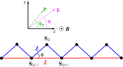
Figure 1: (Color online) Sketch of the sawtooth chain together with the electric field $\mathbf{E}$, the $z$-aligned magnetic field $\mathbf{B}=B\mathbf{e}_{z}$ and the resulting electric polarization $\mathbf{P}$. For the plane defined by the sawtooth geometry the $x$-$y$ plane is chosen.

The MEE in most common terms can be described as the magnetic-field dependence of dielectric polarization and vice versa the electric-field dependence of the magnetization in solids. The origin of the coupling between spins and the dielectric polarization can be very different mee1 ; mee2 ; dong15 ; don19 . The one to be considered in the present paper is based on the so-called spin-current model or inverse Dzyaloshinskii-Moriya (DM) model and is called the Katsura-Nagaosa-Balatsky (KNB) mechanism KNB1 ; KNB2 ; KNB3 . According to the KNB mechanism an electric field can induce a DM term. This term can be obtained by a second-order perturbation theory starting from a Hubbard-like model with spin-orbit coupling.  The electric field leads to a modification of the hopping terms and to the emergence of new hopping paths.  As a result, the KNB mechanism links the dielectric polarization corresponding to a pair of spins at adjacent lattice sites with the following expression:

$$\mathbf{P}_{ij}=\gamma_{ij}\;\mathbf{e}_{ij}\times\mathbf{S}_{i}\times\mathbf{S}_{j},$$ (1.1)

where $\mathbf{e}_{ij}$ is the unit vector pointing from site $i$ to site $j$ and $\gamma_{ij}$ is a microscopic parameter characterizing the quantum chemical features of the bond between two ions with spins $\mathbf{S}_{i}$ and $\mathbf{S}_{j}$ KNB1 ; KNB3 ; KNB2 . Over the past 15 years numerous theoretical studies on quantum spin models with KNB mechanism have been published, see, e.g., bro13 ; Berakdar2014 ; Berakdar2016 ; Berakdar2017 ; thakur18 ; XYZ ; White2020 ; mench15 ; sznajd18 ; sznajd19 ; baran18 ; oles ; stre20 ; oha20 . Interestingly, for various one-dimensional unfrustrated models with the KNB-mechanism an exact solution is possible, see bro13 ; XYZ ; oha20 ; mench15 ; baran18 ; oles .

In recent years, there is a growing interest in the realization of the magnetoelectric effect in low-dimensional magnetic compounds. A prominent class of these (quasi-)one-dimensional materials is given by edge-shared cuprates with ferromagnetic (FM) nearest-neighbor ($J_{1}<0$) and antiferromagnetic (AFM) next-nearest neighbor ($J_{2}>0$) interactions between the Cu²⁺ ions carrying spin $1/2$, see, e.g., Refs. mee2 ; LiCuO21 ; LiCu2O21 ; LiCu2O22 ; LiCuVO44 ; LiVCuO41 ; LiVCuO42 ; LiCuO23 ; Enderle2005 ; KBK:PRB06 ; Drechsler2007 ; LiCuVO43 .

At the same time, many different frustrated spin-lattice models in dimension $D=1,2,3$ were found, where the lowest band of one-magnon excitations above the FM vacuum is dispersionless (flat) lm5 ; lm5a . Caused by the flat band a number of unconventional features emerge in magnetic fields, such as a magnetization jump at the saturation field $B_{\rm sat}$ 2 ; lm4 , a magnetic-field driven spin-Peierls instability spin-peierls , magnon-crystallization in $D=2$ lm2 ; lm2a ; prl2020 , a finite residual entropy at $B_{\rm sat}$ lm2 ; lm3 ; lm2a ; lm5 ; lm5a , a very strong magnetocaloric effect lm2a ; cool2004 ; lm5 , and an additional low-temperature maximum of the specific heat signaling the occurrence of an additional low-energy scale lm5 ; lm5a . Below we will demonstrate that due to the magnetoelectric coupling there are electric analogues to the above mentioned magnetization jump and the enhanced magnetocaloric effect.

A prototype flat-band model is the sawtooth (or delta) chain that has been widely investigated for different realizations such as frustrated quantum spin systems, see, e.g. 2 ; lm2 ; lm3 ; lm4 ; lm5 ; sawt2008 ; FAF1 ; lm8 ; lm9 ; FAF2 ; dre20 ; McClarty2020 ; Pujol2020 ; Hatsugai2020 , electronic systems, see, e.g., Refs. 25 ; 26 ; 27 ; 28 ; 29 ; hubb2010 ; 31 ; 32 ; maimaiti2017 ; 33 ; Katsura_delta1 ; Katsura_delta2 as well as photonic lattices, see, e.g. Refs. photonic ; 34 .

In the present paper we consider the Heisenberg spin-half sawtooth chain coupled to a $z$-aligned magnetic field $\mathbf{B}$ (Zeeman term) and to an electric field $\mathbf{E}$ (KNB term) with arbitrary direction but located within the plane defined by the sawtooth geometry. The corresponding Hamiltonian is given by

$$\mathcal{H} = J_{1}\sum_{j=1}^{N/2}\mathbf{S}_{2j-1}\cdot\mathbf{S}_{2j+1}+J_{2}\sum_{j=1}^{N/2}\mathbf{S}_{2j}\cdot\left(\mathbf{S}_{2j-1}+\mathbf{S}_{2j+1}\right)$$ (1.2)

$$-BM-\mathbf{E}\cdot\mathbf{P}\;,\;\mathbf{B}=B\mathbf{e}_{z}\;,\;M=S_{z}=\sum_{j=1}^{N}S_{j}^{z},$$

$$\mathbf{P} = \sum_{j=1}^{N/2}\mathbf{P}_{2j-1,2j+1}+\sum_{j=1}^{N/2}\left(\mathbf{P}_{2j-1,2j}+\mathbf{P}_{2j,2j+1}\right),$$ (1.3)

see Fig. 1 for the arrangement of spins and bonds as well as the electric and magnetic fields. While we consider AFM $J_{1}$, the zigzag bond $J_{2}$ can be AFM or FM, however, restricted to the region $2J_{1}\leq J_{2}\leq-2J_{2}$, where flat-band physics is possible. In case of zero electric field, for this model two flat-band scenarios are known: For the AFM sawtooth chain, $J_{1},J_{2}>0$, the lowest band of one-magnon excitations above the fully polarized FM state $|\rm FM\rangle=|\uparrow\uparrow\uparrow\ldots\rangle$ is dispersionless for $J_{2}=2J_{1}$ (flat-band point) lm2 ; lm3 ; lm4 ; lm5 ; lm6 ; lm8 ; lm9 . As a result there exist localized multi-magnon states (also called flat-band states) for $N/4\leq S_{z}<N/2$, which are the lowest states in the respective sectors of $S_{z}$. At half of the saturation magnetization, $S_{z}=N/4$, there is a wide plateau and the plateau state is a magnon-crystal state 2 . All the flat-band states are linearly independent lin_indep and their number growths exponentially with the number of sites $N$. In magnetic fields close to saturation the flat-band states dominate the low-temperature thermodynamics of the model lm2 ; lm3 ; lm4 ; lm5 ; lm6 ; lm8 ; lm9 . The experimental observation is not straightforward because the relevant physics typically takes place at (very) high magnetic fields. For a possible experimental realization of an alternative flat-band spin system, where the saturation field is accessible, see Tanaka2014 ; bil2018 .

The second flat-band scenario is realized for the sawtooth Heisenberg chain with FM bonds between the apical and basal spins ($J_{2}<0$) and AFM bonds ($J_{1}>0$) within the basal line FAF1 ; FAF4 ; FAF5 ; FAF3 ; FAF_field . Here, the flat-band point where the lowest band of one-magnon excitations above the fully polarized FM state is dispersionless is given by $J_{2}=-2J_{1}$ FAF1 . Notably, the flat-band states exist here in all magnetization sectors $0\leq S_{z}<N/2$, and again they are the lowest states in the respective magnetization sectors. The number of flat-band states growths even faster exponentially with $N$ than for the first (purely AFM) flat-band scenario leading again to the dominance of these states at low $T$ FAF1 ; FAF3 ; lm9 . A striking difference to scenario 1 is that flat-band physics takes place at zero-magnetic field which enhances the chance to observe the flat-band physics in an experiment. Indeed, there are magnetic compounds which are well described by the FM-AFM sawtooth spin chain, such as malonate-bridged copper complexes FAF7 ; FAF8 and the very recently synthesized and studied magnetic molecule Fe₁₀Gd₁₀ FeGd . While the parameter situation in the former one is not very close to the flat-band point, the Fe₁₀Gd₁₀ molecule exhibits exchange parameters close to the flat-band point FeGd , and, therefore signatures of flat-band physics are well seen in this system FeGd ; FAF3 ; FAF_field .

Further examples for magnetic compounds with sawtooth chain geometry of exchange bonds are the atacamite Cu₂Cl(OH)₃ atacamite , the fluoride Cs₂LiTi₃F₁₂ fluoride , the euchroite Cu₂(AsO₄)(OH)$\cdot$3H₂O euchroite , the sawtooth spin ring Mo₇₅V₂₀ Mo75V20 , the frustrated [Mn₁₈] magnetic wheel-of-wheels molecule Mn18 and the iron compound Fe₂Se₂O₇ sawtooth_exp_2021 .

I.1 Summary of results

The key target of the present paper is the study of the interplay of the KNB mechanism and magnetic frustration at and in the vicinity of a flat-band point. As mentioned above, for the model at hand at zero electric field the realization of flat-band physics requires fine tuning of the exchange parameters, i.e., the very existence of a strictly flat one-magnon band appears only at two singular ratios $J_{2}/J_{1}$. Naively, one may expect that the presence of the electric field leading to additional DM terms in the Hamiltonian eliminates flat-band phenomena.

• A crucial finding of our work is that actually just the electric field via the KNB mechanism may dissolve the fine tuning of $J_{1}$ and $J_{2}$ and can lead to a large variety of $J_{1}$-$J_{2}$ ratios, where for appropriate direction and magnitude of $\mathbf{E}$ the lowest one-magnon band is flat.

• Thus, for a certain system at hand with given values of $J_{1}$ and $J_{2}$ we can achieve flat-band physics by application of an appropriate value of the electric field $E_{\rm f}(J_{1},J_{2})$ (flat-band field).

• Moreover, the saturation field $B_{\rm sat}$ in the vicinity of which the flat-band physics can be observed is lower in the presence of an electric field than for the previously studied flat-band situation at zero electric field 2 ; lm2 ; lm5 ; lm5a , this way leading to a better access to flat-band physics in experiments.

• The flat-band effects known from previous studies 2 ; lm2 ; lm5 ; lm5a without electric field, such as a macroscopic magnetization jump at saturation field, the huge degeneracy of the ground states at the flat-band point leading to a residual entropy, the emergence of an extra-low energy scale in the vicinity the flat-band point as well as an enhanced magnetocaloric effect are also present in case of the electric-field driven flat-band physics.

• In addition to these flat-band phenomena, the presence of an electric field leads to intriguing reciprocal effects: macroscopic jumps in the electric polarization $P$ driven by magnetic field $B$ and macroscopic jumps in the magnetization $M$ driven by the electric field $E$, i.e., there is an extraordinary MEE.

• Last but not least, besides an enhanced magnetocaloric effect known for flat-band magnets there is an enhanced electrocaloric effect. If considering adiabatic cooling for isentropes with entropy $s$ below the residual entropy $s_{\rm res}\sim 0.24$, the temperature drops quickly to zero when approaching $E=E_{\rm f}(J_{1},J_{2})$.

II KNB mechanism for the sawtooth chain

In this section we specify the KNB mechanism for the sawtooth-chain geometry. We choose the $x$ axis along the basal line of $J_{1}$ bonds and the $x$-$y$ plane for the location of the $J_{1}$-$J_{2}$-$J_{2}$ triangle, where the angle between $J_{1}$ and $J_{2}$ bonds is $\theta$, see Fig. 1. The unit vectors along the exchange bonds entering Eq. (1.1) read

$$\mathbf{e}_{2j-1,2j+1}=\mathbf{e}_{x},$$ (2.4)

$$\mathbf{e}_{2j-1,2j}=\cos\theta\;\mathbf{e}_{x}+\sin\theta\;\mathbf{e}_{y},$$

$$\mathbf{e}_{2j,2j+1}=\cos\theta\;\mathbf{e}_{x}-\sin\theta\;\mathbf{e}_{y}.$$

Then the corresponding local polarization vectors are given by

$$\mathbf{P}_{2j-1,2j}=\gamma\left(\cos\theta\mathbf{e}_{x}+\sin\theta\mathbf{e}_{y}\right)\times\mathbf{S}_{2j-1}\times\mathbf{S}_{2j},$$

$$\mathbf{P}_{2j,2j+1}=\gamma\left(\cos\theta\mathbf{e}_{x}-\sin\theta\mathbf{e}_{y}\right)\times\mathbf{S}_{2j}\times\mathbf{S}_{2j+1},$$

$$\mathbf{P}_{2j-1,2j+1}=\gamma^{\prime}\mathbf{e}_{x}\times\mathbf{S}_{2j-1}\times\mathbf{S}_{2j+1},$$ (2.5)

where a different KNB parameter $\gamma^{\prime}=\alpha\gamma$ is considered for the polarization in the basal line taking care of the possibility to have different microscopic quantum-chemical parameters of the KNB mechanism for different exchange bonds. We can merge the first two relations of the Eqs. (II) by rewriting them appropriately in one equation:

$$\mathbf{P}_{j,j+1}=\gamma\left(\cos\theta\;\mathbf{e}_{x}-(-1)^{j}\sin\theta\;\mathbf{e}_{y}\right)\times\mathbf{S}_{j}\times\mathbf{S}_{j+1}.\quad$$ (2.6)

Note that this expression coincides with the one considered for the $XY$ zigzag chain in Ref. baran18 . For an electric field $\mathbf{E}=(E_{x},E_{y},0)$ residing in the $x$-$y$ plane, see Fig. 1, the interaction between the polarization and the electric field entering the Hamiltonian (1.2) reads

$$- \mathbf{E}\cdot\mathbf{P}$$

$$= \sum_{j=1}^{N}\left(\gamma E_{y}\cos\theta+(-1)^{j}\gamma E_{x}\sin\theta\right)\left(S_{j}^{x}S_{j+1}^{y}-S_{j}^{y}S_{j+1}^{x}\right)$$

$$+ \alpha\gamma E_{y}\sum_{j=1}^{N/2}\left(S_{2j-1}^{x}S_{2j+1}^{y}-S_{2j-1}^{y}S_{2j+1}^{x}\right).$$

Note that for this specific combination of the $x$- and $y$-components of the spin operator $\mathbf{S}_{i}$ the Hamiltonian (1.2) commutes with the $z$-component of the total spin, $S_{z}$.

For convenience, we absorb the KNB constant $\gamma$ in $\mathbf{E}$, which in turn is measured in appropriate units. The observables relevant for the MEE are the expectation values of the $x$ and $y$ components of total polarization and the $z$-aligned magnetization:

$$P_{x} = \frac{\sin\theta\langle\sum_{j=1}^{N}(-1)^{j}\left(S_{j}^{y}S_{j+1}^{x}-S_{j}^{x}S_{j+1}^{y}\right)\rangle}{N},$$

$$P_{y} = \frac{\cos\theta\langle\sum_{j=1}^{N}\left(S_{j}^{y}S_{j+1}^{x}-S_{j}^{x}S_{j+1}^{y}\right)\rangle}{N},$$

$$-\alpha\;\frac{\langle\sum_{j=1}^{N/2}\left(S_{2j-1}^{x}S_{2j+1}^{y}-S_{2j-1}^{y}S_{2j+1}^{x}\right)\rangle}{N},$$

$$M = M_{z}=\frac{\langle\sum_{j=1}^{N}S_{j}^{z}\rangle}{N},$$ (2.8)

where $\langle\cdot\rangle$ denotes either the expectation value with respect to a specific state or the thermal average.

Let us mention here, that the considered interaction term (II) can be also understood as DM interaction $\mathbf{D}_{i}=D_{i}\mathbf{e}_{z}$, $i=1,2,3$, with

$$D_{1}=\alpha E\sin\phi,$$ (2.9)

$$D_{2}=E(\sin\phi\cos\theta-\cos\phi\sin\theta),$$

$$D_{3}=E(\sin\phi\cos\theta+\cos\phi\sin\theta),$$

where $D_{1}$ belongs to the basal bonds, and $D_{2}$ and $D_{3}$ belong to the two zigzag bonds, respectively. Such a DM term could be relevant for spin lattices with low symmetry.

III Electric field induced flat bands

In this section we will figure out how the lowest one-magnon band can be flat also in the presence of an electric field. We start with the fully polarized FM state $|FM\rangle=|\uparrow\uparrow\ldots\uparrow\rangle$ which is the ground state for strong enough magnetic field $B$. Imposing periodic boundary conditions we construct one-magnon excitations above the magnon vacuum $|FM\rangle$

$$|1_{k}\rangle=\sum_{l=0,1}a_{l}\sum_{j=1}^{N/2}e^{i\;jk}S_{2j+l}^{-}|FM\rangle,$$ (3.10)

where $k$ is the quasi-momentum. The calculation of the two branches (according to the two sites per unit cell) of the one-magnon spectrum is straightforward:

$$\varepsilon^{\pm}(k)=B-\frac{J_{1}+2J_{2}}{2}+\frac{1}{2}\left[\widetilde{J}_{1}\cos(k-k_{1})\pm\sqrt{\left(J_{1}-\widetilde{J}_{1}\cos(k-k_{1})\right)^{2}+2\widetilde{J}_{2}\widetilde{J}_{3}\cos(k-k_{2}-k_{3})+\widetilde{J}_{2}^{2}+\widetilde{J}_{3}^{2}}\right]\;$$ (3.11)

$$\widetilde{J}_{1}=\sqrt{J_{1}^{2}+D_{1}^{2}},\widetilde{J}_{2}=\sqrt{J_{2}^{2}+D_{2}^{2}},\widetilde{J}_{3}=\sqrt{J_{2}^{2}+D_{3}^{2}},k_{1}=\arctan\frac{D_{1}}{J_{1}},k_{2}=\arctan\frac{D_{2}}{J_{2}},k_{3}=\arctan\frac{D_{3}}{J_{2}}.$$ (3.12)

Because the expression for the spectrum (3.11) is a bit cumbersome due to the phase shifts $k_{i}$, we will consider two special cases for which simplified expressions for $\varepsilon^{\pm}(k)$ are obtained that enable to extract criteria in analytical form for the very existence of flat-band physics.

III.1 Flat-band case I

Here we consider an electric field pointing along the $x$-axis, i.e., $\phi=0$. In this case we have $D_{1}=0$, $D_{2}=-D_{3}=-E\sin\theta$ yielding for the phase shifts $k_{1}=0$ and $k_{2}=-k_{3}$, and the one-magnon dispersion then reads

$$\varepsilon^{\pm}(k)=B-\frac{J_{1}+2J_{2}}{2}+\frac{1}{2}\Big{(}J_{1}\cos k$$ (3.13)

$$\pm\sqrt{J_{1}^{2}(1-\cos k)^{2}+2(J_{2}^{2}+E^{2}\sin^{2}\theta)(1+\cos k)}\Big{)}.$$

Obviously, this expression is very similar to the known standard cases, namely replacing $J_{2}^{2}+E^{2}\sin^{2}\theta$ by an effective coupling $J_{2,\text{eff}}^{2}$ we just obtain the expression for the $k$-dependent term for the pure Heisenberg model without KNB terms, see, e.g., Eq. (3) in sawt2008 . Thus, one gets a flat band if the $x$-aligned electric field obeys the relation

$$E=E_{\rm f}=\pm\frac{\sqrt{4J_{1}^{2}-J_{2}^{2}}}{\sin\theta}.$$ (3.14)

This equation also implies that a flat band driven by an electric field does exist for arbitrary values of $J_{1}$ and $J_{2}$ with the constraint $4J_{1}^{2}\geq J_{2}^{2}$.

Inserting (3.14) in Eq. (3.13) we obtain:

$$\varepsilon^{+}(k) = B+J_{1}-J_{2}+J_{1}\cos k$$

$$\varepsilon^{-}(k) = B-2J_{1}-J_{2}.$$ (3.15)

This yields for the saturation (flat-band) field

$$B_{\rm f}=B_{\rm sat}=2J_{1}+J_{2},$$ (3.16)

which is lower than the corresponding value $B_{\rm sat}=4J_{1}$ for the standard AFM flat-band case. Let us mention that the above discussed flat-band scenario also corresponds to a purely magnetic system without electric field, i.e., for the $J_{1}$-$J_{2}$ Heisenberg sawtooth chain with a staggered DM-interaction term in $z$-direction along the zigzag $J_{2}$ bonds, $D\sum_{j=1}^{N}(-1)^{j}\left(S_{j}^{x}S_{j+1}^{y}-S_{j}^{y}S_{j+1}^{x}\right)$, if $D=\sqrt{4J_{1}^{2}-J_{2}^{2}}$.

We conclude that the above outlined case I for the model at hand opens the window for a flexible access to flat-band physics via the KNB mechanism, because no fine-tuning of the exchange parameters $J_{1}$ and $J_{2}$ is necessary. Moreover, the reduced saturation field also improves the possibility to have experimental access to flat-band physics.

III.2 Flat-band case II

Let us consider a second specific case allowing a simplification of Eq. (3.11). It is given if the electric field is directed parallel to the zigzag bonds, i.e., either $\phi=\pm\theta$ or $\phi=\pm(\pi-\theta)$. Without loss of generality we will take the sign to be plus. The corresponding DM terms become $D_{1}=\alpha E\sin\theta$, $D_{2}=0$, and $D_{3}=2E\sin\theta\cos\theta$ which leads to $\widetilde{J}_{2}=J_{2}$ and $k_{2}=0$ in Eqs. (3.11) and (3.12). A flat band is possible if the remaining phase shifts $k_{1}$ and $k_{2}$ in Eq. (3.11) are equal, i.e.,

$$J_{2}=\frac{2\cos\theta}{\alpha}J_{1}.$$ (3.17)

Finally, the lower band of the one-magnon excitations becomes flat for

$$E=\pm\frac{2J_{1}\sqrt{\cos^{2}\theta-\alpha^{2}}}{\alpha^{2}\sin\theta}\;,\;|\alpha|\leq|\cos\theta|.$$ (3.18)

Obviously, the possible values for $\alpha$ are restricted by the bond angle $\theta$. As in the previous case the two signs of $E$ correspond to the symmetry $\theta\rightarrow-\theta$, $E\rightarrow-E$. Note, however, that for $\phi=-\theta$, the DM-terms in the zigzag part of the chain will be non-zero for odd zigzag-bonds, and we have $D_{1}=-\alpha E\sin\theta$, $D_{2}=-2E\sin\theta\cos\theta$, and $D_{3}=0$.

Again it is appropriate to mention that the above discussed flat-band scenario also corresponds to a purely magnetic system without electric field, i.e., for the $J_{1}$-$J_{2}$ Heisenberg sawtooth chain with specific DM terms, namely uniform DM-interaction along the basal line and non-zero DM-terms only for the even bond on the zigzag line,

$$D_{a}\sum_{j=1}^{N}(1\pm(-1)^{j})\left(S_{j}^{x}S_{j+1}^{y}-S_{j}^{y}S_{j+1}^{x}\right)$$ (3.19)

$$+D_{b}\sum_{j=1}^{N/2}\left(S_{2j-1}^{x}S_{2j+1}^{y}-S_{2j-1}^{y}S_{2j+1}^{x}\right)\;,\;\frac{D_{a}}{D_{b}}=\frac{J_{2}}{J_{1}}.$$

Then the flat band is realized for $D_{a}=\pm\sqrt{J_{2}^{2}-4J_{1}^{2}}$.

We may conclude that by contrast to case I the above outlined flat-band scenario II is less promising with respect to a possible experimental realization because the precondition of fine-tuning of the exchange parameters $J_{1}$ and $J_{2}$ is not removed.

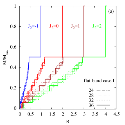
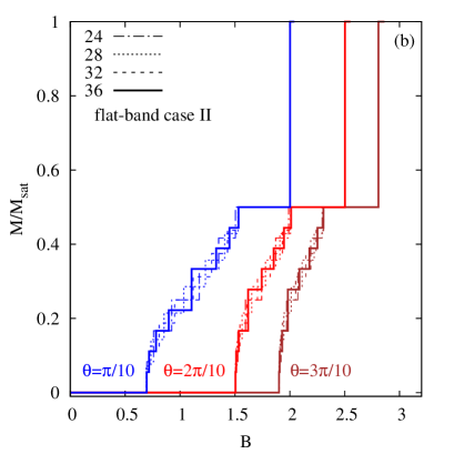
Figure 2: (Color online) GS data of the magnetization $M/M_{\rm sat}$ as a function of the magnetic field $B$ for $N=24,28,32,36$. (a) Flat-band case I (i.e., $\phi=0$) with $\theta=\pi/8$, $J_{1}=1$ and various values of $J_{2}$. (b) Flat-band case II (i.e., $\phi=\theta$) with $\alpha=1/2$ and three values of $\theta$ (obeying $|\alpha|\leq|\cos\theta|$, see Eq. (3.18)) and $\sqrt{J_{1}^{2}+J_{2}^{2}}=1$.

IV Numerical results

We will focus here on case I as the promising case that does not require fine-tuning of $J_{1}$ and $J_{2}$. Case II will be discussed only secondarily. Having in mind, that for case I the value of the bond angle enters the Hamiltonian via $E\sin\theta$ only, cf. Eqs. (2.9) and (3.14), we will show in what follows numerical data for one example of the bond angle, namely $\theta=\pi/8$.

We use the exact diagonalization method (ED) to determine the ground state (GS) as well as finite-temperature properties for finite chains with periodic boundary conditions. To exploit translational symmetry we perform the ED calculations using Jörg Schulenburg’s spinpack code 49 ; 50 .

The ED is a well established quantum many-body technique which is widely applied to frustrated quantum spin systems. It is especially appropriate for one-dimensional systems, because one can apply the ED to a set of finite systems with various numbers of spins $N$. Thus, by comparing systems with different $N$ the finite-size effects can be controlled. Moreover, from previous studies 2 ; FAF1 ; Accuracy2020 it is known that finite-size effects can be particularly small for the sawtooth spin chain. In the present paper we calculate the GS up to $N=36$ by using the Lanczos method and the thermodynamics by calculating the full spectrum up to $N=20$.

In addition to the ED we apply the approximate finite-temperature Lanczos method (FTLM) to calculate thermodynamic properties of larger chains $N>20$. FTLM is a Monte-Carlo like extension of the full ED. Thermodynamic quantities are determined using trace estimators 51 ; 52 ; 53 ; 54 ; 55 ; 56 ; 57 ; 58 ; 59 ; 61 ; 62 . The partition function $Z$ is approximated by a Monte-Carlo like representation of $Z$, i.e., the sum over a complete set of $(2s+1)^{N}$ basis states entering $Z$ is replaced by a much smaller sum over $R$ random vectors $\,|\,{\nu}\,\rangle$ for each subspace ${\mathcal{H}}(S_{z})$ of the Hilbert space.

Figure 3: (Color online) MEE for flat-band case I (i.e., $\phi=0$) with $\theta=\pi/8$, $J_{1}=1$ and various values of $J_{2}$. The numbers in the legend denote the system size $N$. (a) Electric polarization $P=\sqrt{P_{x}^{2}+P_{y}^{2}}$ as function of the magnetic field $B$ for $E=E_{\rm f}$. (b) Magnetization $M$ as function of the electric field $E$ for $B=1.01B_{\rm sat}$.

IV.1 Ground-state properties

We start with the flat-band case I and consider the magnetization curve $M(B)$ first, see Fig. 2(a). $M(B)$ is typical for the known standard (i.e., $E=0$) AFM flat-band case 2 ; sawt2008 : There is a wide plateau at $M/M_{\rm sat}=1/2$ preceeding the jump to saturation. The jump is size-independent. Moreover, the dependence of the width of the plateau on the system size is very weak. Only when approaching the standard FM-AFM flat-band case (i.e., $J_{2}\to-2J_{1}$) FAF1 the plateau shrinks and finally the jump takes place directly from $M=0$ to $M=M_{\rm sat}$. Below the plateau the finite-size steps in $M(B)$ become smaller with growing $N$, and the magnetization curve gets finally smooth without peculiarities as $N\to\infty$.

As for the standard AFM flat-band case there is a massively degenerated ground-state manifold at the saturation field which is built by the localized localized multi-magnon (flat-band) states leading to a residual entropy per site of $s_{\rm res}=\frac{1}{2}\ln\frac{1+\sqrt{5}}{2}=0.240606$ lm2 ; lm3 . Thus we conclude that the GS properties of the flat-band system driven by an electric field $E$ are identical to those of the well-studied AFM flat-band system in absence of $E$.

We mention here that for the flat-band case II the GS flat-band physics at $B=B_{\rm sat}$ is identical to case I, i.e., the magnetization jump and the magnon-crystal plateau are also present, see Fig. 2(b). Moreover, the residual entropy at $B=B_{\rm sat}$ is the same for cases I and II.

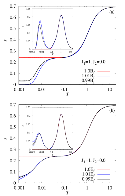
Figure 4: (Color online) Entropy $s=S/N$ (main panel) and specific heat $c=C/N$ (inset) for the flat-band case I with $J_{1}=1$, $J_{2}=0$, $\phi=0$, and $\theta=\pi/8$ for $N=20$ (full ED, short dashes), $N=28$ (FTLM, long dashes) and $N=36$ (FTLM, solid) at and near the flat-band point $B=B_{\rm f}=B_{\rm sat}=2.0$ and $E=E_{\rm f}=2/\sin(\theta)$. (a): $E=E_{\rm f}$, $B=1.01B_{\rm f}$, $1.0B_{\rm f}$, and $B=0.99B_{\rm f}$. (b) $B=B_{\rm f}=2$, $E=1.01E_{\rm f}$, $1.0E_{\rm f}$, and $E=0.99E_{\rm f}$. Note, that the curves for different $N$ almost coincide.

The flat-band induced size-independent discontinuous change of $M(B)$ upon crossing $B_{\rm f}$ leads to similar abrupt changes of $P(B)$ when $B$ traverses the flat-band point $B_{\rm f}$. On the other hand, the electric field $E$ drives a jump-like behavior of the magnetization $M(E)$. Since all these jumps are related to the very existence of a flat-band we may expect that also the jumps in $P(B)$ and $M(E)$ will exhibit at most only small finite-size effects. We demonstrate this in Fig. 3. In the upper panel (a) we show the electric polarization $P$ as a function of the magnetic field $B$ for $J_{1}=1$, $\theta=\pi/8$ and various $J_{2}$ values, where the electric field $E$ is set to the flat-band value $E_{\rm f}$ given by Eq. (3.14). Indeed, we observe a jump of $P$ at $B=B_{\rm sat}$ that amounts to more than 50% of the initial value $P$ at $B=0$. As expected, finite-size effects are very small. In the lower panel (b) we show the magnetization $M$ as a function of the electric field $E$ for $J_{1}=1$, $\theta=\pi/8$ and various $J_{2}$ values, where the magnetic field is set to $B=1.01B_{\text{sat}}$, i.e., for values of the electric field below the flat-band value $E_{\rm f}$ the GS is the fully polarized FM state. When $E$ crosses $E_{\rm f}$ we find a jump down to about 60% of saturation. Interestingly, the jump is even larger for larger $N$. We may conclude that discontinuous changes in $M(E)$ and $P(H)$ most likely remain for $N\to\infty$. Thus, we found evidence of an extraordinarily enhanced MEE with an abrupt change of $M$ (resp. $P$) when varying the electric (resp. magnetic) field due to the very existence of a flat band in the spin system at hand. This provides the opportunity of switching the magnetization by an electric field or the electric polarization by a magnetic field.

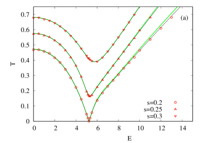
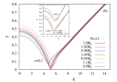
Figure 5: (Color online) (a) Finite-size effects of the electrocaloric effect for the flat-band case I ($\phi=0$, $\theta=\pi/8$, $B=B_{\rm f}$) for $J_{1}=1$ and $J_{2}=0$ (green lines – $N=12$, black lines – $N=16$, red symbols – $N=24$). Isentropes are shown for $s=S/N=0.2$, $0.25$, and $0.3$. (b) Main panel: The electrocaloric effect (isentropes for $s=S/N=0.2$) for the flat-band case I shown for magnetic field $B$ at various values below and above the flat-band value $B_{\rm f}$ for a chain of size $N=12$. Inset: Finite-size effects of the electrocaloric effect shown for isentropes for $s=S/N=0.2$ and $0.3$ (lines – $N=12$, red symbols – $N=24$).

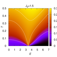
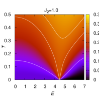
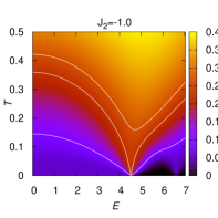
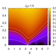
Figure 6: (Color online) Electrocaloric effect (ECE) for the flat-band case I ($\phi=0$, $\theta=\pi/8$, $B=B_{\rm f}$) $J_{1}=1$ and $J_{2}=1.5$, $1.0$, $-1.0$, $-1.5$. The white lines represent isentropes for $s=S/N=0.27$, $0.23$ and $0.1$.

IV.2 Finite-temperature properties

Again, we focus on flat-band case I. As shown by previous studies lm2 ; sawt2008 ; lm5 ; lm5a ; FAF1 ; FAF3 ; lm9 the flat-band states dominate the low-temperature thermodynamics at the flat-band point $E=E_{\rm f}$ and $B=B_{\rm f}=B_{\rm sat}$ as well as in the vicinity of it. This is related to the fact that the flat-band (localized multi-magnon) states build a massively degenerate GS manifold at the flat-band point, and, that in a sizeable parameter region around $E=E_{\rm f}$ and $B=B_{\rm f}$ this former GS manifold acts as a huge manifold of low-lying excitations setting an extra low-energy scale.

This is evident by the temperature profile of the entropy as shown exemplarily in the main panels of Fig. 4, (a) and (b), for $J_{1}=1$, $J_{2}=0$ and a few values of $B$ (resp. $E$) at and in the vicinity of the flat-band value $B_{\rm f}$ (resp. $E_{\rm f}$). The pronounced low-temperature plateaus in $s(T)$ are caused by the manifold of flat-band states, where the width of these plateaus depends on the distance to $B_{\rm f}$ and $E_{\rm f}$, i.e. on $|B-B_{\rm f}|$ and on $|E-E_{\rm f}|$, respectively. The curves for $N=20$, $28$ and $36$ practically coincide down to very low temperatures $T$. Only below $T\sim 0.005$ small finite-size effects appear, i.e. the $s(T)$ profiles shown for various chain length $N$ are slightly different. The small magnitude of finite-size effects can be attributed to the set of flat-band states which scale systematically with system size lm5 ; lm5a . Note that for $N\to\infty$ we get $s(T\to 0)=0$ except for the flat-band point, where the system exhibits a non-zero residual entropy. The different temperature regimes in the $s(T)$ profile are also obvious in the specific heat $c(T)=T\left({\frac{\partial S}{\partial T}}\right)$, see the insets in Fig. 4, (a) and (b). At $E=E_{\rm f}$, $B=B_{\rm f}$ (red curves in Fig. 4) the huge ground-state manifold leads to a vanishing specific heat at low $T$, whereas slightly away from the flat-band point the additional Schottky-like peak in the $c(T)$ profile indicates the extra low-energy scale. It is worth mentioning that, interestingly, for the contribution of the flat-band states to the partition function explicit analytical formulas can be found which describe the low-temperature physics near the flat-band point very well lm2 ; sawt2008 ; lm5 ; lm5a ; FAF1 ; lm9 .

Next, we study the electrocaloric effect (ECE) which currently attracts enormous attention as a promising new approach for refrigeration technologies science2006 ; science2008 ; science2017 ; nano2019 ; science2020 . From previous studies we know that due to the large residual entropy at the flat-band point an enhanced magnetocaloric effect is observed when traversing the saturation field (flat-band point) FAF1 ; cool2004 ; lm2 ; lm5 ; lm5a ; 63 ; 64 ; 65 . Consequently, we may expect an extraordinary ECE when pinning the magnetic field at $B=B_{\rm f}$ and varying the electric field $E$ through the flat-band value $E_{\rm f}$. To verify this we study adiabatic cooling, i.e., the isentropic variation of the temperature when changing the electric field. Computationally that is demanding, since an extensive $T-E$ scan is needed to pin the entropy $s=S/N$ at a predefined value. Fortunately, again the finite-size effects are very small as demonstrated in Fig. 5. Thus we performed extensive simulations of adiabatic cooling for a small system of $N=12$ to create contour plots of the ECE, see Fig. 6. As already shown in Fig. 5 and in more detail demonstrated by the contour plots for $J_{2}=1.5,1.0,-1.0,-1.5$, the variation of the electric field through the flat-band value $E_{\rm f}$ leads to a strong change of temperature. In particular, when considering isentropes with $s$ below the residual entropy $s_{\rm res}\sim 0.24$, the temperature rapidly drops to zero when approaching $E=E_{\rm f}$. Obviously, the general shape of the isentropes does not depend on $J_{2}$. However, the flat-band values $B_{\rm f}$ and $E_{\rm f}$ depend on $J_{2}$, see Eqs. (3.16) and (3.14). With respect to a possible realization of such a flat-band induced enhanced ECE in magnetic compounds the question arises whether there is still an extraordinary ECE, even if the ideal flat-band condition is not fulfilled. For that we show in Fig. 5(b) adiabatic cooling by varying the electric field when pinning the magnetic field $B$ at various values below and above the flat-band value $B_{\rm f}$. Obviously, the ECE remains enhanced; varying the electric field around $E_{\rm f}$ leads to a pronounced downturn of the temperature.

V Conclusion

This paper connects frustrated quantum magnetism (a traditional research field in solid state physics) and the Katsura-Nagaosa-Balatsky (KNB) mechanism to couple spin degrees of freedom to an electric field (a more recent research field in solid state physics) hereby opening the possibility to study flat-band effects in quantum magnets by applying an appropriate electric field. Prominent effects related to the interplay of frustration and the KNB mechanism are strongly enhanced magnetoelectric and electrocaloric effects.

As an example, we consider a specific quantum spin model, the spin-half $J_{1}$-$J_{2}$ sawtooth Heisenberg chain (see Fig. 1). The sawtooth spin chain is a paradigmatic frustrated quantum spin model that can serve as the relevant spin model for various magnetic compounds FAF7 ; FAF8 ; FeGd ; atacamite ; fluoride ; euchroite ; Mo75V20 ; Mn18 such as the recently studied Fe₁₀Gd₁₀ FeGd , Cu₂Cl(OH)₃ atacamite and Fe₂Se₂O₇ sawtooth_exp_2021 .

Although, we consider a idealized strictly one-dimensional model we know from experimental studies azurite_exp_2005 ; azurite_exp_2005_b ; Tanaka2014 that the discussed flat-band effects, such as magnetization jumps, can be seen in real magnetic compounds. Moreover, several theoretical studies for models violating the flat-band condition, i.e. models with (slightly) dispersive bands, demonstrate that flat-band effects are present in considerable parameter region around the flat-band point Jeschke_azurit2011 ; azurite_Hon2011 ; azurite_Derzhko2012 ; beyond_flat2014 ; hubbard_nearly_flat2016 ; richter_sawtooth2020 .

The large variety of frustrated quantum magnetic insulators as well as the progress in synthesizing new magnetic molecules and compounds with predefined spin lattices may open the window to get access to the observation of the discussed phenomena. We expect that the strength of the electric field necessary for that can be achieved since typical exchange couplings are of the order of a few to a hundred kelvin which corresponds to $1\dots 10$ meV. Depending on the KNB constant $\gamma$ this could translate into field strengths applicable to the typically insulating quantum spin materials where a breakdown voltage of 10-30 MV/m could possibly be achieved. We mention here the very recent experimental study of Kocsis et al. switsching2021 for LiCoPO₄ in an electric field of $E\sim 1$ MV/m, where a switching of magnetic states in LiCoPO₄ has been reported.

Further we mention that the discussed electric-field driven flat-band physics also exists for more general sawtooth-chain models, e.g. models with two different zigzag bonds $J_{2}$ and $J_{3}$ including different XXZ anisotropies on all three bonds. Moreover, the flat one-magnon band is also present for corresponding models with $s>1/2$ work_in_progress . The investigation of the generalized sawtooth model and of other flat-band spin systems, e.g. lm5 ; lm5a , promises a rich future of combined effects of frustration and KNB mechanism.

VI Acknowledgments

We thank Hoshu Katsura for illuminating comments on the applicability of the KNB mechanism on spin systems. We also thank Paul McClarty and Alexei Andreanov for critical reading the manuscript. We thank Hiroyuki Nojiri for sharing his knowledge on breakdown voltages with us. V.O. expresses his deep gratitude to the MPIPKS for warm hospitality during his two-month stay in Dresden. V. O. also acknowledges the partial financial support form ANSEF (grant PS-condmatth-2462) and CS RA MESCS (grant 21AG-1C047). J.R. and J.S. thank the DFG for financial support (grants RI 615/25-1 and SCHN 615/28-1).

References

- (1) M. Fiebig, Journal of Physics D: Applied Physics 38, R123 (2005).
- (2) N. A. Spaldin, M. Fiebig and M. Mostovoy, J. Phys.: Condens. Matter 20, 434203 (2008).
- (3) C. Ederer and C. J. Fennie, J. Phys.: Condens. Matter 20, 434219 (2008).
- (4) V. Garcia, M. Bibes, L. Bocher, S. Valencia, F. Kronast, A. Crassous, X. Moya, S. Enouz-Vedrenne, A. Gloter, D. Imhoff, C. Deranlot, N. D. Mathur, S. Fusil, K. Bouzehouane, A. Barthélémy, Science 327, 1106 (2010).
- (5) Y. Tokura, S. Seki, and N. Nagaosa, Rep. Prog. Phys. 77, 076501 (2014).
- (6) Y. Wang, J. Li, D. Viehland, Mater. Today 17, 269 (2014).
- (7) Sh. Dong, J.-M. Liu, S.-W. Cheong, Zh. Ren, Adv. Phys. 64, 519 (2015).
- (8) M. Fiebig, T. Lottermoser, D. Meier, and M. Trassin, Nat. Rev. Mater. 1, 16046 (2016).
- (9) N. A. Spaldin, R. Ramesh, Nat. Mater. 18, 203 (2019).
- (10) Sh. Dong, H. Xiang, and E. Dagotto, Nat. Sci. Rev. 6, 629 (2019).
- (11) S.-W. Cheong and M. Mostovoy, Nature Materials 6, 13 (2007).
- (12) Y. Tokura and S. Seki, Advanced Materials 22, 1554 (2010).
- (13) J. Liu, V. V. Laguta, K. Inzani, W. Huang, S. Das, R. Chatterjee, E. Sheridan, S. M. Griffin, A. Ardavan, R. Ramesh, Sci. Adv. 7, eabf8103 (2021).
- (14) P. Mellado, A. Concha, and S. Rica, Phys. Rev. Lett. 125, 237602 (2020).
- (15) J. F. Scott, Annu. Rev. Mater. Res. 41, 229 (2011).
- (16) A.S. Mischenko, Q. Zhang, J.F. Scott, R.W. Whatmore, N.D. Mathur, Science 311, 1270 (2006).
- (17) B. Neese, B.J. Chu, S.G. Lu, Y. Wang, E. Furman, Q.M. Zhang, Science 321, 821 (2008).
- (18) Mengwei Si, Atanu K. Saha, Pai-Ying Liao, Shengjie Gao, Sabine M. Neumayer, Jie Jian, Jingkai Qin, Nina Balke, Haiyan Wang, Petro Maksymovych, Wenzhuo Wu, Sumeet K. Gupta, and Peide D. Ye, ACS Nano 13, 8760 (2019).
- (19) R. Ma, Z. Zhang, K. Tong, D. Huber, R. Kornbluh, Y. S. Ju, Q. Pei, Science 357, 1130 (2017).
- (20) Y. Wang, Z. Zhang, T.Usui, M. Benedict, S. Hirose, J. Lee, J. Kalb, D. Schwartz, Science 370, 129 (2020).
- (21) D.C. Tsui, H.L. Stormer, and AS.C. Gossard, Phys. Rev. Lett. 48, 1559 (1982).
- (22) H. Tasaki, Phys. Rev. Lett., 69, 1608 (1992).
- (23) A. Mielke, H. Tasaki, Commun. Math. Phys., 158, 341 (1993).
- (24) H. Tasaki, J. Stat. Phys., 84, 535 (1996).
- (25) J. Schulenburg, A. Honecker, J. Schnack, J. Richter, and H.-J. Schmidt, Phys. Rev. Lett. 88, 167207 (2002).
- (26) J. Richter, O. Derzhko, and J. Schulenburg, Phys. Rev. Lett. 93, 107206 (2004).
- (27) M. E. Zhitomirsky and H. Tsunetsugu, Phys. Rev. B 70, 100403(R) (2004).
- (28) S. D. Huber and E. Altman, Phys. Rev. B 82, 184502 (2010).
- (29) H. Katsura, I. Maruyama, A. Tanaka, and H. Tasaki, EPL 91, 57007 (2010).
- (30) K. Sun, Z. Gu, H. Katsura, and S. DasSarma, Phys. Rev. Lett. 106 236803 (2011).
- (31) Gyu-Boong Jo, J. Guzman, C.K. Thomas, P. Hosur, A. Vishwanath, and D.M. Stamper-Kurn, Phys. Rev. Lett. 108, 045305 (2012).
- (32) J. Struck, C. Ölschläger, M. Weinberg, P. Hauke, J. Simonet, A. Eckardt, M. Lewenstein, K. Sengstock, and P. Windpassinger, Phys. Rev. Lett. 108, 225304 (2012).
- (33) E.J. Bergholtz and Zhao Liu, Int. J. Mod. Phys. B 27, 1330017 (2013).
- (34) S. A. Parameswaran, R. Roy, and S. L. Sondhi, C. R. Phys. 14, 816 (2013).
- (35) D. Leykam, S. Flach, O. Bahat-Treidel, and A. S. Desyatnikov, Phys. Rev. B 88, 224203 (2013).
- (36) O. Derzhko, J. Richter, and M. Maksymenko, Int. J. Mod. Phys. 29, 1530007 (2015).
- (37) R.A. Vicencio, C. Cantillano, L. Morales-Inostroza, B. Real, C. Mejía-Cortés, S. Weimann, A.Szameit, and M.I. Molina, Phys. Rev. Lett. 114, 245503 (2015).
- (38) S. Mukherjee, A. Spracklen, D. Choudhury, N. Goldman, P. Öhberg, E. Andersson, and R.R. Thomson, Phys. Rev. Lett. 114, 245504 (2015).
- (39) Y. Cao, V. Fatemi, S. Fang, K. Watanabe, T. Taniguchi, E. Kaxiras, and P. Jarillo-Herrero, Nature 556, 43 (2018).
- (40) D. Leykam, A. Andreanov, and S. Flach, Adv. Phys.: X 3, 1473052 (2018).
- (41) L. Tang, D. Song, S. Xia, Shiqiang Xia, J. Ma, W. Yan, Yi Hu, J. Xu, D. Leykam, and Z. Chen, Nanophotonics 9, 1161 (2020).
- (42) M. Serlin, C. L. Tschirhart, H. Polshyn, Y. Zhang, J. Zhu, K. Watanabe, T. Taniguchi, L. Balents, A.F. Young, Science 367, 900 (2020).
- (43) L. Balents, C. R. Dean, D. K. Efetov, and A. F. Young Nat. Phys. 16, 725 (2020).
- (44) P. Stepanov, I. Das, X. Lu, A. Fahimniya, K. Watanabe, T. Taniguchi, F. H. L. Koppens, J. Lischner, L. Levitov, and D. K. Efetov Nature 583, 375 (2020).
- (45) R. Okuma, D. Nakamura, T. Okubo, A. Miyake, A. Matsuo, K. Kindo, M. Tokunaga, N. Kawashima, S. Takeyama, and Z. Hiroi, Nat. Commun. 10, 1229 (2019).
- (46) J. Schnack, J. Schulenburg, A. Honecker, and J. Richter Phys. Rev. Lett. 125, 117207 (2020).
- (47) H. Katsura, N. Nagaosa, and A. V. Balatsky, Phys. Rev. Lett. 95, 057205 (2005).
- (48) H. Katsura, Nevill F. Mott Prize Lecture at the SCES 2016, Hangshou (May 2016).
- (49) C. Jia, S. Onoda, N. Nagaosa, and J. H. Han, Phys. Rev. B 74, 224444 (2006).
- (50) M. Brockmann, A. Klümper, and V. Ohanyan, Phys. Rev. B 87, 054407 (2013).
- (51) M. Azimi, L. Chotorlishvili, S. K. Mishra, S. Greschner, T. Vekua, and J. Berakdar, Phys. Rev. B 89, 024424 (2014).
- (52) M. Azimi, M. Sekania, S. K. Mishra, L. Chotorlishvili, Z. Toklikishvili, and J. Berakdar, Phys. Rev. B 94, 064423 (2016).
- (53) S. Stagraczynski, L. Chotorlishvili, M. Schüler, M. Mierzejewski, and J. Berakdar, Phys. Rev. B 96, 054440 (2017).
- (54) P. Thakur, P. Durganandini, Phys. Rev. B 97, 064413 (2018).
- (55) T.-Ch. Yi, W.-L. You, N. Wu, and A. M. Oleś, Phys. Rev. B 100, 024423 (2019).
- (56) N. Reynolds, A. Mannig, H. Luetkens, C. Baines, T. Goko, R. Scheuermann, L. Keller, M. Bartkowiak, A. Fujimura, Y. Yasui, Ch. Niedermayer, and J. S. White, Phys. Rev. B 99, 214443 (2019).
- (57) V. Ohanyan, Condens. Matter Phys. 23, 43704 (2020).
- (58) O. Menchyshyn, V. Ohanyan, T. Verkholyak, T. Krokhmalskii, and O. Derzhko, Phys. Rev. B 92, 184427 (2015).
- (59) J. Sznajd, Phys. Rev. B 97, 214410 (2018).
- (60) J. Sznajd, J. Magn. Magn. Mater. 479, 254 (2019).
- (61) O. Baran, V. Ohanyan, and T. Verkholyak, Phys. Rev. B 98, 064415 (2018).
- (62) W.-L. You, G.-H. Liu, P. Horsch, and A. M. Oleś, Phys. Rev. B 90, 094413 (2014).
- (63) J. Strečka, L. Gálisová, and T. Verkholyak, Phys. Rev. E 101, 012103 (2020).
- (64) M. Enderle, C. Mukherjee, B. Fak, R.K. Kremer, J.-M. Broto, H. Rosner, S.-L. Drechsler, J. Richter, J. Malek, A. Prokofiev, W. Assmus, S. Pujol, J.-L. Raggazoni, H. Rakato, M. Rheinstädter, and H.M. Ronnow, EPL 70, 237 (2005).
- (65) R. Klingeler, B. Büchner, K.-Y. Choi, V. Kataev, U. Ammerahl, A. Revcolevschi, J. Schnack, Phys. Rev. B 73, 014426 (2006).
- (66) S. Park, Y. J. Choi, C. L. Zhang, and S.-W. Cheong, Phys. Rev. Lett. 98, 057601 (2007).
- (67) S.-L. Drechsler, O. Volkova, A.N. Vasiliev, N. Tristan, J. Richter, M. Schmitt, H. Rosner, J. Málek, R. Klingeler, A.A. Zvyagin, and B. Büchner, Phys. Rev. Lett. 98, 077202 (2007).
- (68) Y. Yasui, Y. Naito, K. Sato, T. Moyoshi, M. Sato, and K. Kakurai, J. Phys. Soci. Japan 77, 023712 (2008).
- (69) F. Schrettle, S. Krohns, P. Lunkenheimer, J. Hemberger, N. Büttgen, H.-A. Krug von Nidda, A. V. Prokofiev, and A. Loidl, Phys. Rev. B 77, 144101 (2008).
- (70) S. Seki, Y. Yamasaki, M. Soda, M. Matsuura, K. Hirota, and Y. Tokura, Phys. Rev. Lett. 100, 127201 (2008).
- (71) A. S. Moskvin, Yu. D. Panov, S.-L. Drechsler, Phys. Rev. B 79, 104112 (2009).
- (72) A. S. Moskvin, S.-L. Drechsler, EPL 81, 57004 (2008).
- (73) Y. Yasui, K. Sato, Y. Kobayashi, and M. Sato, J. Phys. Soc. Jpn. 78, 084720 (2009).
- (74) Y. Qi and A. Du, Phys. Lett. A 378, 1417 (2014).
- (75) O. Derzhko, J. Richter, Eur. Phys. J. B 52, 23 (2006).
- (76) O. Derzhko, J. Richter, A. Honecker, and H.-J. Schmidt, Low Temp. Phys. 33, 745 (2007).
- (77) J. Richter, J. Schulenburg, A. Honecker, J. Schnack, and H. J. Schmidt, J. Phys.: Condens. Matter 16, S779 (2004).
- (78) M. E. Zhitomirsky and H. Tsunetsugu, Prog. Theor. Phys. Suppl. 160, 361 (2005).
- (79) O. Derzhko and J. Richter, Phys. Rev. B 70, 104415 (2004).
- (80) M. E. Zhitomirsky and A. Honecker, J. Stat. Mech., P07012 (2004).
- (81) J. Richter, O. Derzhko, A. Honecker, Int. J. Modern Phys. B 22, 4418 (2008).
- (82) V. Ya. Krivnov, D. V. Dmitriev, S. Nishimoto, S.-L. Drechsler, and J. Richter, Phys. Rev. B 90, 014441 (2014).
- (83) A. Metavitsiadis, C. Psaroudaki, and W. Brenig, Phys. Rev. B 101, 235143 (2020).
- (84) O. Derzhko, J. Schnack, D. V. Dmitriev, V. Ya. Krivnov, J. Richter, Eur. Phys. J. B 93, 161 (2020).
- (85) T. Yamaguchi , S.-L. Drechsler, Y. Ohta , and S. Nishimoto, Phys. Rev. B 101, 104407 (2020).
- (86) P. A. McClarty, M. Haque, A. Sen, and J. Richter, Phys. Rev. B 102, 224303 (2020).
- (87) Y. Kuno, T. Mizoguchi, and Y. Hatsugai Phys. Rev. B 102, 241115(R) (2020).
- (88) S. Acevedo, P. Pujol, C.A. Lamas Phys. Rev. B 102, 195139 (2020).
- (89) D. V. Dmitriev and V. Ya. Krivnov, J. Phys.: Condens. Matter 28, 506002 (2016).
- (90) Y. Watanabe and S. Miyashita, J. Phys. Soc. Jpn., 66, 2123 (1997).
- (91) R. Arita, Y. Shimoi, K. Kuroki, and H. Aoki, Phys. Rev. B, 57, 10609 (1998).
- (92) O. Derzhko, J. Richter, A. Honecker, M. Maksymenko, and R. Moessner, Phys. Rev. B 81, 014421 (2010).
- (93) M. Maksymenko, A. Honecker, R. Moessner, J. Richter, and O. Derzhko, Phys. Rev. Lett., 109, 096404 (2012).
- (94) S. Flach, D. Leykam, J. D. Bodyfelt, P. Matthies, and A. S. Desyatnikov, EPL, 105, 30001 (2014).
- (95) W. Maimaiti, A. Andreanov, H. C. Park, O. Gendelman, and S. Flach, Phys. Rev. B 95, 115135 (2017).
- (96) W. Zhang, R. Liu, and W. Nie, Science Bulletin, 64, 1490 (2019).
- (97) K. Tamura and H. Katsura, Phys. Rev. B 100, 214423 (2019).
- (98) K. Tamura and H. Katsura, J. Stat. Phys. 182, 16 (2021).
- (99) S. Weimann, L. Morales-Inostroza, B. Real, C. Cantillano, A. Szameit, and R. A. Vicencio, Opt. Lett. 41, 2414 (2016).
- (100) H.-J. Schmidt, J. Richter, R. Moessner, J. Phys. A.: Math. Gen. 39, 10673 (2006).
- (101) H. Tanaka, N. Kurita, M. Okada, E. Kunihiro, Y. Shirata, K. Fujii, H. Uekusa, A. Matsuo, K. Kindo, and H. Nojiri, J. Phys. Soc. Jpn. 83, 103701 (2014).
- (102) J. Richter, O. Krupnitska, V. Baliha, T. Krokhmalskii, and O. Derzhko, Phys. Rev. B 97, 024405 (2018).
- (103) T. Tonegawa and M. Kaburagi, J. Magn. Magn. Mater. 272-276, 898 (2004).
- (104) M. Kaburagi, T. Tonegawa, and M. Kang, J. Appl. Phys. 97, 10B306 (2005).
- (105) D. V. Dmitriev, V. Ya. Krivnov, J. Richter, and J. Schnack, Phys. Rev. B 99, 094410 (2019).
- (106) D. V. Dmitriev, V. Ya. Krivnov, J. Schnack, and J. Richter, Phys. Rev. B 101, 054427 (2020).
- (107) C. Ruiz-Perez, M. Hernandez-Molina, P. Lorenzo-Luis, F. Lloret, J. Cano, and M. Julve, Inorg. Chem. 39, 3845 (2000).
- (108) Yuji Inagaki, Yasuo Narumi, Koichi Kindo, Hikomitsu Kikuchi, Tomohisa Kamikawa, Takashi Kunimoto, Susumu Okubo, Hitoshi Ohta, Takashi Saito, Masaki Azuma, Mikio Takano, Hiroyuki Nojiri, Makoto Kaburagi, and Takashi Tonegawa, J. Phys. Soc. Jpn. 74, 2831 (2005).
- (109) A. Baniodeh, N. Magnani, Y. Lan, G. Buth, C. E. Anson, J. Richter, M. Affronte, J. Schnack, and A. K. Powell, npj Quantum Mater. 3, 10 (2018).
- (110) L. Heinze, H. O. Jeschke, I. I. Mazin, A. Metavitsiadis, M. Reehuis, R. Feyerherm, J.-U. Hoffmann, M. Bartkowiak, O. Prokhnenko, A. U. B. Wolter, X. Ding, V. S. Zapf, C. Corvalan Moya, F. Weickert, M. Jaime, K. C. Rule, D. Menzel, R. Valenti, W. Brenig, S. Süllow, Phys. Rev. Lett. 126, 207201 (2021).
- (111) R. Shirakami, H. Ueda, H. O. Jeschke, H. Nakano, S. Kobayashi, A. Matsuo, T. Sakai, N. Katayama, H. Sawa, K. Kindo, C. Michioka, and K. Yoshimura, Phys. Rev. B 100, 174401 (2019).
- (112) H. Kikuchi, Y. Fujii, D. Takahashi, M. Azuma, Y. Shimakawa, T. Taniguchi, A. Matsuo and K. Kindo, J. Phys. Conf. Series 320, 12045 (2011).
- (113) Y. Oshima, H. Nojiri, J. Schnack, P. Kögerler, M. Luban, Phys. Rev. B 85, 024413 (2012).
- (114) M. Coletta, T. G. Tziotzi, M. Gray, G. S. Nichol, M. K. Singh, C. J. Milios and E. K. Brechin, Chemical Communications (2021) DOI:10.1039/D1CC00185J.
- (115) K. Nawa, M. Avdeev, P. Berdonosov, A. Sobolev I. Presniakov, A. Aslandukova, E. Kozlyakova, A. Vasiliev, I. Shchetinin, and T. J. Sato, Sci. Rep. 11, 24049 (2021).
- (116) J. Schulenburg, spinpack-2.59 , Magdeburg University (2019).
- (117) J. Richter and J. Schulenburg, Eur. Phys. J. B 73, 117 (2010).
- (118) J. Schnack, J. Richter, and R. Steinigeweg, Phys. Rev. Research 2, 013186 (2020).
- (119) J. Jaklic and P. Prelovsek, Phys. Rev. B 49, 5065 (1994).
- (120) J. Jaklic and P. Prelovsek, Adv. Phys. 49, 1 (2000).
- (121) A. Hams and H. De Raedt, Phys. Rev. E 62, 4365 (2000).
- (122) J. Schnack and O. Wendland, Eur. Phys. J. B 78, 535 (2010).
- (123) P. Prelovsek and J. Bonca, "Ground State and Finite Temperature Lanczos Methods", in "Strongly Correlated Systems, Numerical Methods", eds. A. Avella and F. Mancini, Springer Series in Solid-State Sciences 176 (Berlin, 2013)
- (124) O. Hanebaum and J. Schnack, Eur. Phys. J. B 87, 194 (2014).
- (125) B. Schmidt and P. Thalmeier, Phys. Rep. 703, 1 (2017).
- (126) E. Pavarini, E. Koch, R. Scalettar, and R. M. Martin, eds., ’The physics of correlated insulators, metals, and superconductors’, (2017) Chap. ’The Finite Temperature Lanczos Method and its Applications’ by P. Prelovsek, ISBN 978-3-95806-224-5, http://hdl.handle.net/2128/15283.
- (127) J. Schnack, J. Schulenburg, and J. Richter, Phys. Rev. B 98, 094423 (2018).
- (128) K. Seki and S. Yunoki, Phys. Rev. B 101, 235115 (2020).
- (129) K. Morita and T. Tohyama, Phys. Rev. Research 2, 013205 (2020).
- (130) M. E. Zhitomirsky, Phys. Rev. B 67, 104421 (2003).
- (131) J. Schnack, R. Schmidt, and J. Richter, Phys. Rev. B 76, 054413 (2007).
- (132) B. Wolf, A. Honecker, W. Hofstetter, U. Tutsch, and M. Lang, Int. J. Mod. Phys. B 28, 1430017 (2014).
- (133) H. Kikuchi, Y. Fujii, M. Chiba, S. Mitsudo, T. Idehara, T. Tonegawa, K. Okamoto, T. Sakai, T. Kuwai, and H. Ohta, Phys. Rev. Let. B 94, 227201 (2005).
- (134) H. Kikuchi, Y. Fujii, M. Chiba, S. Mitsudo, T. Idehara, T. Tonegawa, K. Okamoto, T. Sakai, T. Kuwai, K. Kindo, A. Matsuo, W. Higemoto, K. Nishiyama, M. Horvatic and C. Berthier, Prog. Theor. Phys. Suppl. 159, 1 (2005).
- (135) H. Jeschke, I. Opahle, H. Kandpal, R. Valenti, H. Das, T. Saha-Dasgupta, O. Janson, H. Rosner, A. Bruhl, B. Wolf, M. Lang, J. Richter, S. Hu, X. Wang, R. Peters, T. Pruschke, and A. Honecker, Phys. Rev. Lett. 106, 217201 (2011).
- (136) A. Honecker, S. Hu, R. Peters, and J. Richter, J. Phys.: Condens. Matter 23 164211 (2011).
- (137) O. Derzhko, J. Richter, O. Krupnitska, Cond. Matter Phys. 15, 43702 (2012).
- (138) O. Derzhko, J. Richter, O. Krupnitska, and T. Krokhmalski, Low Temp. Phys. 40, 662 (2014).
- (139) P. Müller, J. Richter, and O. Derzhko, Phys. Rev. B 93, 144418 (2016).
- (140) J. Richter, J. Schulenburg, D.V. Dmitriev, V.Ya. Krivnov, and J. Schnack, Cond. Matter Phys. 23, 43710 (2020).
- (141) V. Kocsis, Y. Tokunaga, Y. Tokura, and Y. Taguchi, Phys. Rev. B 104, 054426 (2021).
- (142) V. Ohanyan, J. Richter, and A.Andreanov, work in progress.