Most Classic Problems Remain NP-hard on Relative Neighborhood Graphs and their Relatives

Abstract

Proximity graphs have been studied for several decades, motivated by applications in computational geometry, geography, data mining, and many other fields. However, the computational complexity of classic graph problems on proximity graphs mostly remained open. We now study 3-Colorability, Dominating Set, Feedback Vertex Set, Hamiltonian Cycle, and Independent Set on the proximity graph classes relative neighborhood graphs, Gabriel graphs, and relatively closest graphs. We prove that all of the problems remain $\operatorname{NP}$-hard on these graphs, except for 3-Colorability and Hamiltonian Cycle on relatively closest graphs, where the former is trivial and the latter is left open. Moreover, for every $\operatorname{NP}$-hard case we additionally show that no $2^{o(n^{1/4})}$-time algorithm exists unless the ETH fails, where $n$ denotes the number of vertices.

1 Introduction

Proximity graphs describe the distance relationships between points in the plane or higher-dimensional structures. They are mostly studied in computational geometry, yet arise in several fields of science and engineering [31, 43]: most obviously in geography, less obviously in data mining [18, 29], computer vision [47], the design of mobile ad-hoc networks [3, 39], the design of crowd-movement sensors [14], analyzing road traffic [46], and describing the spread of a species of mold [1]. In this paper, we study the computational complexity of classic NP-complete problems on three specific proximity graphs: relative neighborhood graphs (RNGs) [42], Gabriel graphs (GGs) [23], and relatively closest graphs (RCGs) [34]. All three are subgraphs of the better-known Delaunay triangulation (DT). For DTs, the restrictions of some classic $\operatorname{NP}$-complete graph problems have already been studied [16, 20] and we extend this research to these three classes.

RNGs, GGs, and RCGs are examples of empty region graphs [12]. Every pair of points is associated with a region in the plane, their region of influence, and is connected by an edge if there is no other point in that region (see Fig. 1).

Figure 1: (a) Set $P$ of four points $p_{1}=(0,2)$, $p_{2}=(2,0)$, $p_{3}=(2,3)$, and $p_{4}=(5,3/2)$. (b) RCG on $P$. Point $p_{4}$ is not adjacent with $p_{2}$, since $p_{3}$ lies in the region of influence indicated with green (dashdotted) and red (dashed). (c) RNG on $P$. Points $p_{2}$ and $p_{3}$ are not adjacent since $p_{1}$ is their region of influence indicated with red (dashed) and blue (dotted). (d) GG on $P$. Points $p_{1}$ and $p_{4}$ are not adjacent since $p_{2}$ is in their region of influence indicated with magenta (dashdotted).

In RNGs (RCGs), two points’ region of influence is the intersection of open (closed) circles centered on each of the points with a radius equal to their distance. In a GG, two points’ region of influence is a circle whose center is midway between them and whose diameter is their distance.

Motivation.

In a railway network, it may make sense to build a track directly from one city to another, if there is no third city in between. If we interpret the area between two cities as a region of influence, then this makes proximity graphs such as RNGs plausible models for such networks. One might want to build as few maintenance facilities for the network as possible such that every track has a facility at one of its endpoints. This is an instance of the Vertex Cover (VC) problem (closely related to Independent Set (IS)). While VC is $\operatorname{NP}$-hard on general graphs, one wonders whether it might be easier on proximity graphs. We will show that the problem remains $\operatorname{NP}$-hard on RCGs, RNGs, and GGs.

Related Work.

Existing combinatorial results on the three graph classes include listing forbidden subgraphs, permitted graphs, and bounds on the edge density [8, 17, 31, 37, 45]. Much algorithmic research on proximity graphs has focused on devising algorithms that efficiently compute the proximity graph from a point set (see [38] for an overview). On Delaunay triangulations, Hamiltonian Cycle is $\operatorname{NP}$-hard [20], whereas 3-Colorability is polynomial-time solvable [16]. Cimikowski conjectured 3-Colorability to be NP-hard on RNGs and GGs [15]. Furthermore, he proposed a heuristic for coloring GGs and a linear-time algorithm for computing a $4$-coloring in RNGs, [16] but the latter has some issues, which we will discuss in Section 3.

Our Contributions.

Table 1 summarizes our results.

Table 1: Overview of our results. Herein, $\Delta$ denotes the maximum vertex degree.
^† no $2^{o(n^{1/4})}$-time algorithm exists unless the ETH fails, where $n$ denotes the number of vertices

	RCGs	RNGs	GGs
3-Colorability (3-Col)	trivial	$\operatorname{NP}$-hard†, even if $\Delta=7$  (Thm. 2)
Dominating Set (DS)	$\operatorname{NP}$-hard†, even if $\Delta=4$  (Thm. 6)
Feedback Vertex Set (FVS)	$\operatorname{NP}$-hard†, even if $\Delta=4$  (Thm. 3)
Hamiltonian Cycle (HC)	open	$\operatorname{NP}$-hard†, even if $\Delta=4$  (Thm. 4)
Independent Set (IS)	$\operatorname{NP}$-hard†, even if $\Delta=4$ (Thm. 5)

We prove that 3-Colorability (3-Col), Dominating Set (DS), Feedback Vertex Set (FVS), Hamiltonian Cycle (HC), and Independent Set (IS) are $\operatorname{NP}$-hard on RNGs and GGs, in particular confirming the aforementioned conjecture by Cimikowski [15]. On RCGs 3-Col is trivial, but we prove that DS, FVS, and IS remain $\operatorname{NP}$-hard. All our $\operatorname{NP}$-hardness results hold true even for graphs of fairly small maximum degree (at most seven in the case of 3-Col, and four in all other cases). We complement each $\operatorname{NP}$-hardness result with a running-time lower bound of $2^{o(n^{1/4})}$ based on the Exponential-Time Hypothesis, where $n$ is the number of vertices.

Our Technique.

In our NP-hardness proofs (see Table 1), we give polynomial-time many-one reductions from each problem’s restriction to planar graphs with maximum degree three or four. We proceed as follows (see Fig. 2 for an illustration). We exploit the fact that for any planar graph with maximum degree at most four, we can compute in polynomial time a $2$-page book embedding [5], a very structured representation of the input graph. Then, we translate the book embedding’s structure into a grid-like structure. Each reduction uses three types of gadgets: to represent vertices, to represent edges, and to fill the space between them in order to prevent the appearance of unwanted edges between the other gadgets.

Figure 2: (a) A graph $G$ with vertex set $\{v_{1},\dots,v_{4}\}$. (b) A 1-page book embedding of $G$. (c) and (d) Illustration of our technique, where black rectangles correspond to vertex gadgets, thick gray lines to edge/connector gadgets, and light gray areas indicate filler gadgets.

2 Preliminaries

Let $\mathbb{N}\coloneqq\{1,2,3,\dots\}$ and $\mathbb{N}_{0}\coloneqq\{0\}\cup\mathbb{N}$. We use basic notions from graph theory [19].

Proximity graphs.

Let $\operatorname{d}\colon\mathbb{R}^{2}\times\mathbb{R}^{2}\rightarrow\mathbb{R}$ denote the Euclidean distance between two points. The open and closed ball with radius $r>0$ and center $p\in\mathbb{R}^{2}$ are $B_{r}(p)\coloneqq\{q\in\mathbb{R}^{2}\mid\operatorname{d}(p,q)<r\}$ and $\overline{B}_{r}(p)\coloneqq\{q\in\mathbb{R}^{2}\mid\operatorname{d}(p,q)\leq r\}$. The Delaunay triangulation of $P\subseteq\mathbb{R}^{2}$ (see, e.g., [6, Ch. 9]) is denoted by $\operatorname{DT}(P)$.

A template region [12] is a function $R\colon\binom{\mathbb{R}^{2}}{2}\rightarrow 2^{\mathbb{R}^{2}}$ that assigns a region of the plane, called the region of influence, to each pair of points in the plane. Given a template region $R_{\mathcal{C}}$ and points $p_{1},p_{2}\in\mathbb{R}^{2}$, a third point $p_{3}\in\mathbb{R}^{2}\setminus\{p_{1},p_{2}\}$ is a $\mathcal{C}$-blocker for $\{p_{1},p_{2}\}$ if $p_{3}\in R_{\mathcal{C}}(p_{1},p_{2})$. For a finite set of points $P=\{p_{1},\ldots,p_{n}\}\subseteq\mathbb{R}^{2}$, the $\mathcal{C}$-graph induced by $P$ is $\mathcal{C}(P)\coloneqq(\{v_{1},\ldots,v_{n}\},E_{\mathcal{C}(P)})$ with $E_{\mathcal{C}(P)}\coloneqq\{\{v_{i},v_{j}\}\mid(R_{\mathcal{C}}(p_{i},p_{j})\cap P)\setminus\{p_{i},p_{j}\}=\emptyset\text{ and }i\neq j\}$. The class $\mathcal{C}$ contains a graph $G$ if there is a finite set of points $P\subseteq\mathbb{R}^{2}$ with $\mathcal{C}(P)=G$.

We are interested in three template regions and the graph classes defined by them:

Relatively closest graphs (RCGs):

Defined by

$$R_{\operatorname{RCG}}(p_{1},p_{2}) \coloneqq\{p_{3}\in\mathbb{R}^{2}\mid\operatorname{d}(p_{1},p_{2})\geq\max\{\operatorname{d}(p_{1},p_{3}),\operatorname{d}(p_{2},p_{3})\}\}$$

$$=\overline{B}_{\operatorname{d}(p_{1},p_{2})}(p_{1})\cap\overline{B}_{\operatorname{d}(p_{1},p_{2})}(p_{2}).$$

Relative neighborhood graphs (RNGs):

Defined by

$$R_{\operatorname{RNG}}(p_{1},p_{2}) \coloneqq\{p_{3}\in\mathbb{R}^{2}\mid\operatorname{d}(p_{1},p_{2})>\max\{\operatorname{d}(p_{1},p_{3}),\operatorname{d}(p_{2},p_{3})\}\}$$

$$=B_{\operatorname{d}(p_{1},p_{2})}(p_{1})\cap B_{\operatorname{d}(p_{1},p_{2})}(p_{2}).$$

Gabriel graphs (GGs):

Defined by

$$R_{\operatorname{GG}}(p_{1},p_{2}) \coloneqq\{p_{3}\in\mathbb{R}^{2}\mid\operatorname{d}(p_{1},p_{2})^{2}\geq\operatorname{d}(p_{1},p_{3})^{2}+\operatorname{d}(p_{2},p_{3})^{2}\}$$

$$=\overline{B}_{\operatorname{d}(p_{1},p_{2})/2}(q),$$

where $q$ is the midpoint between $p_{1}$ and $p_{2}$.

A $\mathcal{C}$-embedding of a graph $G=(V,E)$ is a map $\operatorname{emb}\colon V\rightarrow\mathbb{R}^{2}$ such that $\mathcal{C}(\operatorname{emb}(V))=G$. Of course, $G\in\mathcal{C}$ if and only if $G$ admits a $\mathcal{C}$-embedding.

For any finite point set $P$, it holds that $E_{\operatorname{RCG}(P)}\subseteq E_{\operatorname{RNG}(P)}\subseteq E_{\operatorname{GG}(P)}\subseteq\operatorname{DT}(P)$ [17]. RCGs cannot contain $C_{3}$ as a subgraph and none of the three can contain $K_{4}$ or $K_{2,3}$ [17, 37, 45]. Moreover, $p_{3}\in R_{\operatorname{GG}}(p_{1},p_{2})$ if and only if the angle at $p_{3}$ formed by the lines to $p_{1}$ and $p_{2}$ is at least $90\degree$ [37]. Finally, the following lemma will be used to prove that graphs are in each graph class:

Lemma 1 ([37]).

Let $P$ be a set of points in the plane and $G$ the RCG, RNG or GG induced by $P$. Then, the straight-line drawing of $G$ induced by $P$ is planar.

Book embeddings.

Our $\operatorname{NP}$-hardness proofs use 2-page book embeddings. A $k$-page book embedding of a graph $G=(V,E)$ consists of (i) an edge partition $E=E_{1}\uplus\dots\uplus E_{k}$, and (ii) for every $i\in\{1,\ldots,k\}$, a planar embedding $\operatorname{emb}_{i}$ of $(V,E_{i})$ in $\mathbb{R}\times\mathbb{R}_{\geq 0}$, where $\operatorname{emb}_{i}(v)=\operatorname{emb}_{j}(v)\in\mathbb{R}\times\{0\}$ for every $v\in V$, $i,j\in\{1,\ldots,k\}$. The following result due to Bekos et al. [5] will play an important role in this work:

Theorem 1 ([5]).

Every planar graph with maximum degree at most four admits a 2-page book embedding. Such an embedding can be computed in quadratic time.

The following terminology will be useful in our NP-hardness proofs. Consider a graph $G=(V,E)$ and a 2-page book embedding of $G$. Let $v_{1},\ldots,v_{n}$ be the vertices of the graph ordered in such a way that $\operatorname{emb}_{i}(v_{j})<\operatorname{emb}_{i}(v_{j+1})$ for $i\in\{1,2\}$ and every $j\in\{1,\ldots,n-1\}$. We will say that $v_{1},\ldots,v_{n}$ is the order in which the vertices appear on the spine. Let $r\in\{1,2\}$. We will use $N_{r}(v)\coloneqq\{v^{\prime}\,|\,\{v,v^{\prime}\}\in E_{r}\}$ to denote $v$’s $E_{r}$-neighborhood and $\deg_{r}(v)\coloneqq|N_{r}(v)|$ to denote $v$’s $E_{r}$-degree. For an edge $e=\{v_{i},v_{j}\}$, $i<j$, define its length as $\ell(e)\coloneqq j-i$. The interior of $e\in E_{r}$ is

$$\operatorname{int}(e)\coloneqq\{e^{\prime}=\{v_{i^{\prime}},v_{j^{\prime}}\}\in E_{r}\mid i\leq i^{\prime}<j^{\prime}\leq j,e^{\prime}\neq e\}.$$

The $E_{r}$-height of a vertex $v$ is

$$h_{r}(v)\coloneqq\max\{0,h(e)\mid v\in e\in E_{r}\},\quad\text{where}\quad h(e)\coloneqq 1+\max\{0,h(e^{\prime})\mid e^{\prime}\in\operatorname{int}(e)\}$$

denotes the height of $e$. Let $h_{r}(G)\coloneqq\max\{h_{r}(v_{i})\,|\,i\in\{1,\ldots,n\}\}$. Note that, because the height of any edge only depends on the height of shorter edges, edge height is well-defined. The length and height of an edge are both in $\mathcal{O}(n)$. For every vertex $v_{i}$, we order its incident edges in $E_{r}$ as follows. If $N_{r}(v_{i})=\{v_{j_{1}},\ldots,v_{j_{k}}\}$ with $j_{1}<\ldots<j_{c}<i<j_{c+1}<\ldots<j_{k}$, then the order of the edges is $\{v_{i},v_{j_{c}}\}<\ldots<\{v_{i},v_{j_{1}}\}<\{v_{i},v_{j_{k}}\}<\ldots<\{v_{i},v_{j_{c+1}}\}$.

Grid structure.

The graphs we build in our reductions will all have a grid-like structure. With the exception of the reduction for Hamiltonian Cycle, we group their vertices into $(x,y)$-corners with $(x,y)\in\mathbb{Z}^{2}$ and there will be a corner for every $(x,y)$ within certain bounds, which depend on the problem in question as well as the size and structure of the input graph. In the embedding, the vertices forming the $(x,y)$-corner will be in $\overline{B}_{r}(x,y)$ for a suitable $r>0$. Some vertices are not part of any corner and are called intermediate vertices. They are usually located midway between two corners. Each corner can have one or multiple dedicated right, top, left, and bottom connecting vertices. If a corner consists of a single vertex, that vertex always simultaneously acts as the right, top, left and bottom connecting vertex of that corner. The connecting vertices of a corner are the only ones that may have neighbors outside of that corner. For any $(x,y)\in\mathbb{Z}^{2}$, we say that the vertices in the $(x,y)$, $(x+1,y)$, $(x,y+1)$, and $(x+1,y+1)$-corners along with any intermediate vertices that are adjacent to vertices in two of the aforementioned corners jointly form a grid face.

Exponential-Time Hypothesis.

Hypothesis 1 (Exponential-Time Hypothesis (ETH) [30]).

There is some fixed $c>0$ such that 3-CNF-Sat is not solvable in $2^{cn}\cdot(n+m)^{\mathcal{O}(1)}$ time, where $n$ and $m$ denote the numbers of variables and clauses, respectively.

The ETH implies lower bounds for numerous problems. We start by deriving one for Vertex Cover, which is defined as:

Problem 1.

Vertex Cover (VC)

Input: An undirected graph $G=(V,E)$ and $k\in\mathbb{N}_{0}$.

Question: Is there a vertex set $X\subseteq V$ with $\lvert X\rvert\leq k$ such that $G-X$ is edgeless?

We prove an ETH-based lower bound for the following restriction of Vertex Cover.

Lemma 2.

Vertex Cover restricted to planar graphs with maximum degree three admits no $2^{o(n^{1/2})}$-time algorithm where $n$ is number of vertices, unless the ETH fails.

Proof.

Unless the ETH fails, Vertex Cover on planar graphs admits no $2^{o(n^{1/2})}$-time algorithm where $n$ is the number of vertices [35]. There is a reduction [24] from Vertex Cover on planar graphs to the restriction of the same problem to planar graphs with maximum degree three. We present a slightly modified version of this reduction which only changes the number of vertices linearly, thereby proving the claim.

Let $G=(V,E)$ be a planar graph and $k\in\mathbb{N}$. We construct a planar graph $G^{\prime}$ with maximum degree three and an integer $k^{\prime}\in\mathbb{N}$ as follows. For every $v\in V$, let $d\coloneqq\deg_{G}(v)$ and $w_{1},\ldots,w_{d}$ be the neighbors of $v$ in the cyclic order in which the corresponding edges enter $v$. We replace $v$ with a cycle consisting of the vertices $u_{1}^{v},\ldots,u^{v}_{2d}$ in that order and add an additional vertex $z^{v}$. In addition to the edges in the cycle, we add the edges $\{z^{v},u^{v}_{1}\}$ and $\{u^{v}_{2i},w_{i}\}$ for every $i\in\{1,\ldots,d\}$. We set $k^{\prime}\coloneqq k+\sum_{v\in V}\deg_{G}(v)=k+2|E|$. Note that the maximum degree in $G^{\prime}$ is three, that the planarity of $G^{\prime}$ follows from the planarity of $G$, and that both $G^{\prime}$ and $k^{\prime}$ can be computed in polynomial time.

We must show that $G$ contains a vertex cover of size $k$ if and only if $G^{\prime}$ contains a vertex cover size $k^{\prime}$. If $X\subseteq V$ is a vertex cover of size at most $k$, then

$$X^{\prime}\coloneqq\{u^{v}_{1}\mid v\in V\} \cup\{u^{v}_{2i+1}\mid i\in\{1,\ldots,\deg_{G}(v)-1\},v\in V\setminus X\}$$

$$\cup\{u^{v}_{2i}\mid i\in\{1,\ldots,\deg_{G}(v)\},v\in X\}$$

is a vertex cover of size

$$|V|+\sum_{v\in V\setminus X}(\deg_{G}(v)-1)+\sum_{v\in X}\deg_{G}(v) =|V|-|V\setminus X|+\sum_{v\in V}\deg_{G}(v)$$

$$=|X|+\sum_{v\in V}\deg_{G}(v)\leq k^{\prime}.$$

Conversely, suppose that $X^{\prime}$ is a vertex cover of size $k^{\prime}$ in $G^{\prime}$. Then, let $X\coloneqq\{v\in V\mid u^{v}_{2i}\in X\text{ for any }i\in\{1,\ldots,\deg_{G}(v)\}\}$. We claim that $X$ is a vertex cover in $G$. If $\{v,w\}\in E$, then $u_{2i}^{v}$ or $u_{2i^{\prime}}^{w}$ for some $i,i^{\prime}$ must be in $X^{\prime}$ and, hence, $v$ or $w$ is in $X$. It remains to show that $|X|\leq k$. We may assume that $u_{1}^{v}\in X^{\prime}$ for all $v\in V$, since the edge $\{u_{1}^{v},z^{v}\}$ must be covered. For every $v\in V$, let $X^{\prime}_{v}\coloneqq X^{\prime}\cap\{u^{v}_{1},\ldots,u^{v}_{2\deg_{G}(v)}\}$. Because every edge in the cycle representing $v$ is covered, it follows that $|X^{\prime}_{v}|\geq\deg_{G}(v)$. Since $\sum_{v\in V}\lvert X^{\prime}_{v}\rvert=\lvert\bigcup_{v\in V}X^{\prime}_{v}\rvert\leq k^{\prime}=k+\sum_{v\in V}\deg_{G}(v)$, there are at most $k$ vertices with $\lvert X^{\prime}_{v}\rvert>\deg_{G}(v)$. Since $u_{1}^{v}\in X^{\prime}_{v}$ holds, $\lvert X^{\prime}_{v}\rvert=\deg_{G}(v)$ implies that $X^{\prime}_{v}=\{u_{1}^{v},u_{3}^{v},\ldots,u_{2\deg_{G}(v)-1}^{v}\}$. Hence, $\lvert X\rvert\leq k$.

The output graph $G^{\prime}$ contains

$$\sum_{v\in V}(2\deg_{G}(v)+1)=|V|+2\sum_{v\in V}\deg_{G}(v)=|V|+4|E|\in\mathcal{O}(|V|)$$

vertices. Thus, if Vertex Cover on planar graphs with maximum degree three is solvable in $2^{o(n^{1/2})}$ time, then Vertex Cover on arbitrary planar graphs is solvable in $2^{o(n^{1/2})}$ time. ∎

3 3-Colorability

In this section we study the following problem on RCGs, RNGs, and GGs.

Problem 2.

3-Colorability (3-Col)

Input: An undirected graph $G=(V,E)$.

Question: Is there a function $c\colon V\rightarrow\{1,2,3\}$ such that $c(u)\neq c(v)$ for all $\{u,v\}\in E$?

Every RCG is 3-colorable [17] because RCGs do not contain any $3$-cycles and every planar graph without $3$-cycles is $3$-colorable by Grötzsch’s theorem [28]. As a result, 3-Col is trivial when restricted to RCGs. Regarding RNGs and GGs, we prove the following.

Theorem 2.

3-Colorability on RNGs and on GGs is $\operatorname{NP}$-hard, even if the maximum degree is seven. It admits no $2^{o(n^{1/4})}$-time algorithm where $n$ is the number of vertices unless the ETH fails.

This confirms a conjecture by Cimikowski [15]. Our proof is based on a polynomial-time many-one reduction from the $\operatorname{NP}$-hard [25] 3-Colorability on planar graphs with maximum degree four.

Figure 3: A coloring path of length $3$.

We will use so-called coloring paths (see Fig. 3 for an illustration), which essentially allows us to copy the color of a vertex. The coloring path of length $k$ from $u^{1}_{0}$ to $u^{1}_{k}$ is the graph $\tilde{P}_{k}\coloneqq(V_{k},E_{k})$ with:

$$V_{k} \coloneqq\{u^{1}_{0}\}\cup\{u^{1}_{i},u^{2}_{i},u^{3}_{i}\,|\,i\in\{1,\ldots,k\}\}\text{ and }$$

$$E_{k} \coloneqq\{\{u^{1}_{i-1},u^{2}_{i}\},\{u^{1}_{i-1},u^{3}_{i}\},\{u^{2}_{i},u^{3}_{i}\},\{u^{2}_{i},u^{1}_{i}\},\{u^{3}_{i},u^{1}_{i}\}\,|\,i\in\{1,\ldots,k\}\}.$$

We will call $u^{1}_{i}$ the $i$-th center vertex, $u^{2}_{i}$ the $i$-th left vertex, and $u^{3}_{i}$ the $i$-th right vertex.

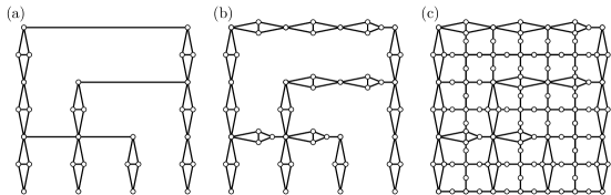
Figure 4: Construction 1 applied to the example graph in Fig. 2. (a) The graph after steps 1–2. (b) The graph after steps 1–3. (c) The final graph.

Construction 1.

Let $G=(V,E)$ be an undirected planar graph of maximum degree four. We will construct a graph $G^{\prime}=(V^{\prime},E^{\prime})$ and subsequently show that $G^{\prime}$ is both an RNG and a GG and that $G$ is $3$-colorable if and only if $G^{\prime}$ is (see Fig. 4 for an illustration). The vertex set of $G^{\prime}$ will mostly consist of groups of vertices called $(x,y)$-corners where $2\leq x\leq 2n$ and $-2h_{2}(G)\leq y\leq 2h_{1}(G)$. Each corner consists of either a single vertex or of a pair of adjacent vertices. Corners can have dedicated top, left, right, and bottom connecting vertices, some of which may coincide. For example, if a corner consists of a single vertex, that vertex simultaneously forms all four connecting vertices. Finally, there will be some intermediate vertices that are not part of any corner. We start with $G^{\prime}\coloneqq G$.

Step 1: Compute a 2-page book embedding of $G$. Let $v_{1},\ldots,v_{n}$ be the vertices of $G$ enumerated in the order in which they appear on the spine, and let $\{E_{1},E_{2}\}$ denote the partition of $E$.

Step 2: Replace every vertex $v_{i}$ with a coloring path of length $h_{1}(v_{i})+h_{2}(v_{i})$. Every edge $e$ of $G$ incident to $v_{i}$ is now instead attached to the $(h_{2}(v_{i})+h(e))$-th center vertex, if $e\in E_{1}$, or the $(h_{2}(v_{i})-h(e))$ if $e\in E_{2}$. For $r=0,\ldots,h_{1}(v_{i})+h_{2}(v_{i})$, the $r$-th center vertex of that path forms the $(2i,2r-2h_{2}(v_{i}))$-corner. For $r=1,\ldots,h_{1}(v_{i})$, the $r$-th left and right vertices jointly form the $(2i,2r-1-2h_{2}(v_{i}))$-corner. The left vertex is the left connecting vertex of this corner and the right vertex is the right connecting vertex.

Step 3: For every edge $e=\{v_{i},v_{j}\}\in E_{1}$, $i<j$, replace the corresponding edge of $G^{\prime}$ with a coloring path of length $\ell(e)$. Identify the first vertex of that path with the $(2i,2h(e))$-corner (which consists of a single vertex). Denote the last vertex of that path by $w$. Add an edge from $w$ to the $(2j,2h(e))$-corner. For $r=1,\ldots,\ell(e)-1$, the $r$-th center vertex of that path is the $(2i+2r,2h(e))$-corner. The vertex $w$, which is the $\ell(e)$-th center vertex, is an intermediate vertex. For $r=1,\ldots,\ell(e)$, the $r$-th left and right vertices jointly form the $(2i+2r-1,2h(e))$-corner. The left vertex is the top connecting vertex of this corner and the right vertex is the bottom connecting vertex.

Step 4: For every $(x,y)$ with $2\leq x\leq 2n$ and $0\leq y\leq 2h_{1}(G)$, if an $(x,y)$-corner was not added in one of the previous two steps, then add a single vertex, which becomes the $(x,y)$-corner, to $G^{\prime}$. In that case add an edge from the $(x,y)$-corner to the top connecting vertex of the $(x,y-1)$-corner, to the left connecting vertex of the $(x+1,y)$-corner, and so on. Subdivide each of these edges once, introducing four new intermediate vertices.

Note that steps 3 and 4 take only $E_{1}$ into account. These steps must be repeated analogously for $E_{2}$, using negative $y$-coordinates. $\diamond$

Lemma 3.

Let $G=(V,E)$ and $G^{\prime}$ be graphs.

1. If $G^{\prime}$ is obtained from $G$ by replacing a vertex $v\in V$ with a coloring path of any length and connecting each $u\in N_{G}(v)$ with one of the center vertices of that coloring path, then $G$ is $3$-colorable if and only if $G^{\prime}$ is.

2. If $G^{\prime}$ is obtained from $G$ by replacing an edge $e=\{u,v\}\in E$ with a coloring path of any length, identifying the first vertex of that path with $u$ and connecting the last vertex of that path to $v$, then $G$ is $3$-colorable if and only if $G^{\prime}$ is.

3. If $v_{1},\ldots,v_{k}\in V$ and $G^{\prime}$ is obtained from $G$ by adding $k+1$ vertices $w,u_{1},\ldots,u_{k}$ and the edges $\{v_{i},u_{i}\}$ and $\{u_{i},w\}$ for every $i=1,\ldots,k$, then, $G$ is $3$-colorable if and only if $G^{\prime}$ is.

4. If $G^{\prime}$ is obtained from $G$ by applying Construction 1 and $n$ is the number of vertices in $G$, then $G^{\prime}$ contains $\mathcal{O}(n^{2})$ vertices.

Proof.

1. Let $\tilde{P}_{k}=(V_{k},E_{k})$ be the coloring path that replaces $v$.

   Suppose that $c\colon V\rightarrow\{1,2,3\}$ is a $3$-coloring of $G$. Without loss of generality assume that $c(v)=1$. Then, $c^{\prime}\colon V^{\prime}\rightarrow\{1,2,3\}$, with $c^{\prime}(u)\coloneqq c(u)$ for all $u\in V\setminus\{v\}$, $c^{\prime}(u_{i}^{1})=1$ for all center vertices $u_{i}^{1}$, $c^{\prime}(u_{i}^{2})\coloneqq 2$ for all left vertices $u_{i}^{2}$, and $c^{\prime}(u_{i}^{3})\coloneqq 3$ for all right vertices $u_{i}^{3}$, is a valid $3$-coloring of $G^{\prime}$.

   Conversely, suppose that $c^{\prime}\colon V^{\prime}\rightarrow\{1,2,3\}$ is a $3$-coloring of $G^{\prime}$. Without loss of generality, assume that $c^{\prime}(u_{0}^{1})=1$. Then, $\{c^{\prime}(u_{1}^{2}),c^{\prime}(u_{1}^{3})\}=\{2,3\}$. Since $u_{1}^{1}$ is adjacent to $u_{1}^{2}$ and $u_{1}^{3}$, it follows that $c^{\prime}(u_{1}^{1})=1$. By induction then $c^{\prime}(u_{i}^{1})=1$ for all $i=1,\ldots,k$. Hence, $c^{\prime}(u)\neq 1~{}$ for all vertices $u\in V\setminus\{v\}$ that are adjacent to $v$ in $G$, since they are adjacent to a center vertex in $G^{\prime}$. Then, $c\colon V\rightarrow\{1,2,3\}$ with $c(v)\coloneqq 1$ and $c(u)\coloneqq c^{\prime}(u)$ for all $u\in V\setminus\{v\}$ is a valid $3$-coloring of $G$.

2. Follows from (i).

3. Suppose that $c\colon V\rightarrow\{1,2,3\}$ is a $3$-coloring of $G$. Let $c^{\prime}\colon V^{\prime}\rightarrow\{1,2,3\}$ with $c^{\prime}(v)\coloneqq c(v)$ for all $v\in V$, $c(w)\coloneqq 3$, and:

   $$c^{\prime}(u_{i})\coloneqq\begin{cases}1,&\text{ if }c(v_{i})\neq 1,\\ 2,&\text{ if }c(v_{i})=1.\end{cases}$$

   Then, $c^{\prime}$ is a valid $3$-coloring of $G^{\prime}$.

   If $G^{\prime}$ is $3$-colorable, then so is $G$, since $G$ is a subgraph of $G^{\prime}$.

4. The graph $G^{\prime}$ contains $\mathcal{O}(n^{2})$ corners each containing $\mathcal{O}(1)$ vertices and $\mathcal{O}(n^{2})$ intermediate vertices.

∎

Proof of Theorem 2.

Steps 2, 3, and 4 of Construction 1 preserve the $3$-colorability of $G^{\prime}$ by Lemma 3(i), (ii), and (iii), respectively. By Lemma 3(iv), the size of the graph $G^{\prime}$ output by the reduction is polynomial in the size of the input graph and it is easy to see that the computations in the construction may be performed in polynomial time. The degree restriction follows from the fact that the construction does not generate any vertices with degree above 7.

It remains to show that $G^{\prime}$ is an RNG and a GG. We start by giving an embedding of $G^{\prime}$. If the $(x,y)$-corner is a single vertex, then its position is $(x,y)$. If the $(x,y)$-corner consists of a left and right vertex that are part of a coloring path added in step 2, then they are embedded at $(x-\varepsilon,y)$ and $(x+\varepsilon,y)$, respectively. If this corner consists of left and right vertices from a coloring path added in step 3, then their embedding is $(x,y+\varepsilon)$ and $(x,y-\varepsilon)$, respectively. Note that each intermediate vertex is adjacent to vertices in exactly two corners. If it is adjacent to the $(x,y)$- and $(x^{\prime},y^{\prime})$-corner, then it is embedded halfway in between, at $(\frac{x+x^{\prime}}{2},\frac{y+y^{\prime}}{2})$.

Figure 5: Grid faces created by Construction 1.

We now show that the RNG and GG induced by the vertices of any grid face is in fact the subgraph of $G^{\prime}$ induced by those vertices. To this end, we show for any pair of vertices sharing a grid face that there is no RNG blocker if they are adjacent and that there is a GG blocker if they are not adjacent. We do this by examining the grid faces individually. Fig. 5 pictures all types of grid faces that may occur in $G^{\prime}$ (up to symmetry).

In the case of the grid face pictured in Fig. 5.(a) the claim is obvious.

In the case of Fig. 5.(b), the vertex $a$ is not an RNG blocker for the edge $\{b,c\}$, because

$$\operatorname{d}(b,c)^{2} =1+\varepsilon^{2}$$

$$\operatorname{d}(a,c)^{2} =1+\left(\frac{1}{2}-\varepsilon\right)^{2}=1+\frac{1}{4}-2\varepsilon+\varepsilon^{2}.$$

Hence, if $\varepsilon>0$ is sufficiently small then $\operatorname{d}(b,c)^{2}<\operatorname{d}(a,c)^{2}$, implying that $a$ is not an RNG blocker for $\{b,c\}$. Similarly,

$$\operatorname{d}(d,b)^{2}=\operatorname{d}(e,b)^{2}=1+\frac{1}{4},$$

implies that $d$ and $e$ also are not an RNG blockers for this edge if $\varepsilon$ is sufficiently small.

For the other grid faces, the claim follows along the same lines.

By Lemma 1, there can be no edges between vertices that do not share a grid face. Thus, we have proven that the given embedding induces $G^{\prime}$ as its RNG and GG.

ETH-lower bound. 3-Col on planar graphs with maximum degree four cannot be solved in $2^{o(n^{1/2})}$ time where $n$ is the number of vertices unless the ETH fails. To show this, we inspect the reduction by [25]. First, it reduces 3-SAT to 3-Col (on arbitrary graphs). This reduction maps formulas with $m$ clauses and $n$ variables to graphs with $\mathcal{O}(m+n)$ vertices and $\mathcal{O}(m+n)$ edges. 3-Col on arbitrary graphs is then reduced to planar 3-Col, mapping graphs with $n$ vertices and $m$ edges to graphs with $\mathcal{O}(n+m^{2})$ vertices and $\mathcal{O}(m^{2})$ edges. Then, 3-Col on arbitrary planar graphs is reduced to 3-Col on planar graphs with maximum degree four. This reduction replaces each vertex $v$ with a subgraph containing $\mathcal{O}(\deg(v))$ vertices and edges. Hence, this reduction maps graphs containing $n$ vertices and $m$ edges to graphs with $\mathcal{O}(m)$ vertices and edges. The composition of these reductions yields a reduction from 3-SAT to 3-Col on planar graph with maximum degree four that maps a formula with $m$ clauses and $n$ variables to a graph containing $\mathcal{O}(m^{2}+n^{2})$ vertices and edges. ∎

We remark that RNGs and GGs with maximum degree three are always $3$-colorable. This follows from Brooks’ theorem [11, 36], which states that any graph with maximum degree $\Delta\geq 3$ which contains no $(\Delta+1)$-clique, is $\Delta$-colorable. RNGs and GGs contain no $4$-cliques (see Section 2). It remains open whether 3-Col can be solved in polynomial time on RNGs or GGs with maximum degree between four and six.

By the well-known $4$-color theorem, all planar graphs are $4$-colorable. The fastest known algorithm to compute a $4$-coloring of a planar graph has quadratic running time [40]. For RNGs, Cimikowski [16] proposed an algorithm for computing $4$-colorings in linear time. However, this algorithm is based on the claim [45] that the wheel graph $W_{6}$ cannot occur as subgraph of an RNG. This claim was disproved by Bose et al. [8]. Cimikowski’s algorithm additionally implicitly assumes that RNGs are closed under minors, since the algorithm sometimes merges two adjacent vertices. This can lead to graphs that are not RNGs. Thus, it remains open whether or not a linear-time algorithm for this task exists.

4 Feedback Vertex Set

In this section, we will study the following problem:

Problem 3.

Feedback Vertex Set (FVS)

Input: An undirected graph $G=(V,E)$ and $k\in\mathbb{N}_{0}$.

Question: Is there a vertex set $X\subseteq V$ with $|X|\leq k$ such that $G-X$ is a forest?

We will show:

Theorem 3.

Feedback Vertex Set on RCGs, on RNGs, and on GGs is $\operatorname{NP}$-hard, even if the maximum degree is four. Unless the ETH fails, it admits no $2^{o(n^{1/4})}$-time algorithm where $n$ is the number of vertices.

Our proof is based on a polynomial-time many-one reduction from the $\operatorname{NP}$-complete [41] Feedback Vertex Set on planar graphs of maximum degree four.

The second part of Theorem 3 is derived from the following.

Observation 1.

Unless the ETH fails, Feedback Vertex Set on planar graphs of maximum degree four admits no $2^{o(n^{1/2})}$-time algorithm where $n$ is the number of vertices.

Proof.

Speckenmeyer [41] proves that FVS is $\operatorname{NP}$-hard on planar graphs with maximum degree four using a series of reductions starting from Vertex Cover on planar graphs with maximum degree four and each of these reductions only introduces a linear change in the number of vertices. Using Lemma 2, this implies that FVS on planar graphs with maximum degree four admits no $2^{o(n^{1/2})}$-time algorithm where $n$ is the number of vertices unless the ETH fails. ∎

Figure 6: Buffer at position $(x,y)\in\mathbb{R}^{2}$ with highlighted outer vertices.

In the reduction, we will use the graph pictured in Fig. 6, which we call a buffer. The highlighted vertices are called outer vertices. We will also use several gadgets to represent vertices in the input graph. The $(4,0)$-, $(3,1)$-, and $(2,2)$-vertex gadgets are pictured in Fig. 7. Each of them contains several buffers. The highlighted vertices in each vertex gadget are called outlets. When referring to them, we will order the outlets in the top and bottom half from left to right, calling them the first top outlet, second top outlet, etc.

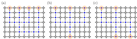
Figure 7: The (a) $(4,0)$-, (b) $(3,1)$-, and (c) $(2,2)$-vertex gadget with highlighted outlets.

We will now give the construction of the reduction from FVS on planar graphs with maximum degree four to FVS on RCGs, RNGs, and GGs.

Figure 8: Construction 2 applied to the graph in Fig. 2. The large blue vertices form a subdivision of the original graph. The bottom half consists of four vertex gadgets, colored alternatingly orange and yellow.

Construction 2.

Let $G=(V,E)$ be a planar graph with maximum degree four and let $k\in\mathbb{N}_{0}$. We will construct a graph $G^{\prime}=(V^{\prime},E^{\prime})$ that is an RCG, an RNG, and a GG, and $k^{\prime}\in\mathbb{N}_{0}$ such that $G$ contains a feedback vertex set of size $k$ if and only if $G^{\prime}$ contains a feedback vertex set of size $k^{\prime}$ (see Fig. 8 for an illustration). The vertex set $V^{\prime}$ will mostly consist of groups of vertices called $(x,y)$-corners, where $5\leq x\leq 9n+4$ and $-2h_{2}(G)-3\leq y\leq 2h_{1}(G)+3$. Each corner consists of either a single vertex or a buffer. In the embedding of $G^{\prime}$, the vertices forming the $(x,y)$-corner will be embedded roughly around the coordinate $(x,y)$. In the case of a buffer, only its outer vertices will have edges to vertices outside of that corner. We refer to them as the top, bottom, left, and right connecting vertices of the corner. If a corner consists of a single vertex, then that vertex itself simultaneously forms the top, bottom, left, and right connecting vertex of that corner. We start with $G^{\prime}\coloneqq G$ and $k^{\prime}\coloneqq k$ and then perform the following steps in order.

Step 1: Compute a 2-page book embedding of $G$. Let $v_{1},\ldots,v_{n}$ be the vertices of $G$ enumerated in the order in which they appear on the spine, and let $\{E_{1},E_{2}\}$ denote the partition of $E$.

Step 2: For each $v_{i}$ add an $(a,b)$-vertex gadget to $G^{\prime}$ such that $a+b=4$, $a\geq\deg_{1}(v_{i})$, and $b\geq\deg_{2}(v_{i})$. Increase $k^{\prime}$ by $4b$ where $b$ is the number of buffers in the vertex gadget. Connect the vertices on the boundary of each gadget to the adjacent gadgets as pictured in the lower half of Fig. 8. The vertices of the gadget representing $v_{i}$ are organized into $(x,y)$-corners where $9i-4\leq x\leq 9i+4$ and $-3\leq y\leq 3$, with the central vertex of that gadget forming the $(9i,0)$-corner. In particular, the $a$ outlets and $9-a$ buffers along the top of the gadget form the $(x,3)$-corners where $9i-4\leq x\leq 9i+4$. Similarly, the $b$ outlets and $9-b$ buffers along the bottom of the gadget form the $(x,-3)$-corners. Recall the order of edges incident to a vertex defined in Section 2. Let $e_{1}<\ldots<e_{\deg_{1}(v_{i})}$ be the edges in $E_{1}$ incident to $v_{i}$ in that order. Then, edge $e_{i}$ is attached to the $i$-th top outlet. The edges in $E_{2}$ are attached to the bottom outlets in the same manner.

Step 3: For every edge $e=\{v_{i},v_{j}\}\in E_{1}$, $i<j$, do the following: Suppose $e$ is $v_{i}$’s $r$-th edge and $v_{j}$’s $s$-th edge according to the order. After $e$ is attached to vertex gadgets in the previous step, $e$ starts at the top connecting vertex of the $(9i+\alpha,3)$-corner and ends at the $(9j+\beta,3)$-corner, where

$$\alpha\coloneqq\begin{cases}2r-5,&\text{ if }\deg_{1}(v_{i})=4,\\ 3r-6,&\text{ if }\deg_{1}(v_{i})\in\{2,3\},\\ 0,&\text{ if }\deg_{1}(v_{i})=1,\end{cases}\qquad\text{and}\qquad\beta\coloneqq\begin{cases}2s-5,&\text{ if }\deg_{1}(v_{j})=4,\\ 3s-6,&\text{ if }\deg_{1}(v_{j})\in\{2,3\},\\ 0,&\text{ if }\deg_{1}(v_{j})=1.\end{cases}$$

Let $L\coloneqq 9\ell(e)-\alpha+\beta-1$ and $d\coloneqq 4h(e)+L$. Subdivide the edge $2d-1$ times and let $w_{1},\ldots,w_{2d-1}$ be the vertices introduced by the subdivision. For every $t\in\{1,\ldots,2h(e)\}$, the vertex $w_{2t}$ is the $(9i+\alpha,3+t)$-corner, and if $t<2h(e)$, the vertex $w_{4h(e)+2L+2t}$ is the $(9j+\beta,3+2h(e)-t+1)$-corner. For every $t\in\{1,\ldots,L\}$, the vertex $w_{4h(e)+2t}$ is the $(9i+\alpha+t,3+2h(e))$-corner. If $t$ is odd, then $w_{t}$ is an intermediate vertex.

Step 4: Add buffers to $G^{\prime}$ as depicted in Fig. 8. More precisely, for each $(x,y)\in\mathbb{N}^{2}$ with $5\leq x\leq 9n+4$ and $4\leq y\leq 2h_{1}(G)+3$, if no $(x,y)$-corner was added in step 3, do the following. Add a buffer, which becomes the $(x,y)$-corner, increase $k^{\prime}$ by $4$, and add an edge connecting the top connecting vertex of the $(x,y)$-corner with the bottom connecting vertex of the $(x,y+1)$-corner, the left connecting vertex of the $(x,y)$-corner with the right connecting vertex of the $(x-1,y)$-corner, and so on. Subdivide each of these edges once, each resulting is an intermediate vertex.

In steps 3 and 4, we have only taken $E_{1}$ into account. These steps must be repeated analogously for the edges in $E_{2}$, using negative $y$-coordinates. $\diamond$

In order to prove the correctness of the reduction, we will need several observations.

Lemma 4.

Let $G$ and $G^{\prime}$ be graphs and let $\varphi(G)$ and $\varphi(G^{\prime})$ denote the size of a smallest feedback vertex set in each graph.

1. If $G^{\prime}$ is obtained from $G$ by subdividing an edge, then $\varphi(G)=\varphi(G^{\prime})$.

2. If $G^{\prime}$ is obtained from $G$ by adding vertices of degree at most one, then $\varphi(G)=\varphi(G^{\prime})$.

3. If $G^{\prime}$ is obtained from $G$ by adding a copy of the buffer graph and connecting each of the outer vertices of the buffer to at most one vertex in $G$, then $\varphi(G^{\prime})=\varphi(G)+4$.

4. If $G^{\prime}$ is the graph obtained by applying Construction 2 to $G$, and $n$ is the number of vertices in $G$, then $G^{\prime}$ contains $\mathcal{O}(n^{2})$ vertices.

Proof.

Parts (i) and (ii) are immediately obvious.

1. Let $X$ be a feedback vertex set in $G$. Then we obtain a feedback vertex set $X^{\prime}$ in $G^{\prime}$ by adding the four degree-4 vertices of the buffer to $X$. Thus $\varphi(G^{\prime})\leq\varphi(G)+4$. Conversely, any feedback vertex set $X^{\prime}$ in $G^{\prime}$ must contain at least 4 vertices from the buffer, as the buffer contains 4 vertex-disjoint cycles. As none of these 4 vertices intersects any cycle in $G$, deleting them from $X^{\prime}$ yields a feedback vertex set for $G$. Thus $\varphi(G)\leq\varphi(G^{\prime})-4$.

2. The graph $G^{\prime}$ contains $\mathcal{O}(n)$ vertex gadgets (each containing a constant number of vertices) and $\mathcal{O}(n^{2})$ corners, each consisting of $\mathcal{O}(1)$ vertices, and $\mathcal{O}(n^{2})$ vertices obtained from the subdivisions in step 5. ∎

We are set to prove the main result of this section.

Proof of Theorem 3.

Each vertex gadget consists of paths from a central vertex to the outlets as well as numerous buffers in addition to vertices that can be introduced by subdividing edges within the gadget. Hence, by Lemma 4, step 2 of Construction 2 is correct. For steps 3 and 4, this also follows from the lemma.

As noted in the same lemma, the size of $G^{\prime}$ is polynomial in the size of $G$. It is easy to see that the computations in Construction 2 can be performed in polynomial time and that there is no vertex of degree greater than 4.

We will argue that $G^{\prime}$ is an RNG. We embed the vertices in the following manner: The vertex gadget representing the vertex $v_{i}$ is embedded using the coordinates given in Fig. 7 with the center vertex located at $(9i,0)$. The $(x,y)$-corner is embedded as shown in Fig. 6 with its center vertex located at $(x,y)$. Intermediate vertices are adjacent to vertices in at most two corners and are embedded halfway between those two corners.

Figure 9: The four types of grid faces in $G^{\prime}$

We must show that there is no RCG blocker for any edge in $G^{\prime}$ and that there is a GG blocker for every pair of non-adjacent vertices. For any $(x,y)\in\mathbb{Z}^{2}$ with $5\leq x<9n+4$ and $-2h_{2}(G)-3\leq y<2h_{1}(G)+3$, the subgraph of $G^{\prime}$ induced by the vertices in the corners $(x,y)$, $(x+1,y)$, $(x,y+1)$, and $(x+1,y+1)$ along with the intermediate vertices adjacent to vertices in those corners will be called a grid face. We start by proving the claim for any two vertices that share a grid face. There are four types of grid faces (up to symmetry), depending on how many of its corners . They are pictured in Fig. 9. In each case, the intermediate vertices are GG blockers for any edges between corners. ∎

Note that FVS is polynomial-time solvable on graphs with maximum degree three [44].

5 Hamiltonian Cycle

In this section, we study the Hamiltonian Cycle problem on RNGs and GGs (for RCGs the complexity will be left open). This problem is defined by:

Problem 4.

Hamiltonian Cycle (HC)

Input: An undirected graph $G=(V,E)$.

Question: Is there a cycle in $G$ visiting every vertex in $V$ exactly once?

We will prove the following:

Theorem 4.

Hamiltonian Cycle on RNGs and on GGs is $\operatorname{NP}$-hard, even if the maximum degree is four. Moreover, unless the ETH fails, it admits no $2^{o(n^{1/4})}$-time algorithm where $n$ is the number of vertices.

To prove Theorem 4, we give a polynomial-time many-one reduction from the restriction of Hamiltonian Cycle to $3$-regular planar graphs, for which we have the following.

Proposition 1 ([26],[35]).

Hamiltonian Cycle on $3$-regular planar graphs is $\operatorname{NP}$-hard and admits no $2^{o(n^{1/2})}$-time algorithm unless the ETH fails.

The reduction in the proof of Theorem 4 consists of two Hamiltonicity-preserving modifications: gadget expansion (Section 5.1) and face filling (Section 5.2).

5.1 Gadget Expansion

Figure 10: The ladder path $L_{4,2}$ with (a) selected vertex labels and inside/outside edges highlighted in dark green / light blue; (b) a traversal; (c) a partial/full cover (light blue / dark green).

The gadgets that will replace the edges are called ladder paths. For $k_{1},k_{2}\in\mathbb{N}$, the ladder path with length $(k_{1},k_{2})$ is the graph $L_{k_{1},k_{2}}=(V_{k_{1},k_{2}},E_{k_{1},k_{2}})$, where

$$V_{k_{1},k_{2}}=\{u^{1}_{i},\tilde{u}^{1}_{i},u^{3}_{i},\tilde{u}^{3}_{i}\mid i\in\{0,\ldots,k_{1}-1\}\}\cup\{u^{2}_{i},\tilde{u}^{2}_{i}\mid i\in\{0,\ldots,k_{2}-1\}\}\cup\{w_{1},\ldots,w_{7}\}$$

and the edges are given using the example pictured in Fig. 10(a). The vertices $u^{j}_{i},\tilde{u}^{j}_{i}$ with $j\in\{1,2\}$ along with $w_{1}$ and $w_{2}$ form the first half of the ladder path and those with $j=3$ along with $w_{4},\ldots,w_{7}$ form the second half. The vertex $w_{3}$ is the transitional vertex. The vertices $w_{1},\ldots,w_{7}$ form the switch. The vertices $u_{0}^{1}$ and $\tilde{u}_{0}^{1}$ form the end of the first half, while $u_{0}^{3}$ and $\tilde{u}_{0}^{3}$ form the end of the second half. The edges highlighted in light blue in Fig. 10(a) will be called outside edges, while the edges highlighted in dark green are inside edges. An edge $\{u^{i}_{j},u^{i}_{j+1}\}$ or $\{\tilde{u}^{i}_{j},\tilde{u}^{i}_{j+1}\}$ is called even if $j$ is even.

A traversal of a ladder path is a path that begins in either vertex at one end of the ladder path, terminates in either vertex at the other end, and visits every vertex on the ladder path and no other vertex. A partial cover of a half of a ladder path is a path that begins in either vertex in the end of the half, terminates in the other vertex in that end, and visits every vertex of that half, but no other vertex. A full cover of a half additionally visits the transitional vertex. Examples of a traversal, a partial, and a full cover are pictured in Fig. 10(b) and (c). The main property of ladder paths is that any Hamiltonian cycle must either contain a traversal, or a full and a half cover of each ladder path.

We will use the following minor technical lemma:

Lemma 5.

Suppose $v_{0},\ldots,v_{n-1}$ is a Hamiltonian cycle in $G$. Then, for any $i,j\in\{1,\ldots,n-2\}$, $i\leq j$, the graph $G-\{v_{i},\ldots,v_{j}\}$ contains no vertex of degree zero or one, except possibly $v_{i-1}$ and $v_{j+1}$.

Proof.

Let $i,j\in\{1,\ldots,n-2\}$, $i\leq j$. Any $v_{k}$, $k\in\{0,\ldots,n-1\}\setminus\{i-1,\ldots,j+1\}$, has at least two neighbors in $G-\{v_{i},\ldots,v_{j}\}$. ∎

Lemma 6.

Suppose that the Hamiltonian graph $G=(V,E)$ contains a ladder, that the only vertices on the ladder path with neighbors outside of the ladder path are on its ends, and that the vertices on the ends each have no more than one neighbor outside of the ladder path. Then, any Hamiltonian cycle in $G$ contains either:

• a traversal of the ladder path or

• a partial cover of one of its halves and a full cover of the other half.

Proof.

Consider any Hamiltonian cycle $C$ in $G$ and any copy of the ladder path $L_{k_{1},k_{2}}$ in $G$. In this Hamiltonian cycle, the vertex $w_{3}$ is succeeded by $w_{1}$, $w_{2}$, $w_{4}$, or $w_{5}$. By symmetry, we assume without loss of generality that the successor is $w_{1}$ or $w_{2}$. We will only deal with $w_{1}$ being the successor as the argument for $w_{2}$ is very similar. The successor of $w_{1}$ is in turn either $w_{2}$ or $u_{k_{2}-1}^{2}$.

For the first case, assume that $w_{1}$’s successor is $w_{2}$. Then $w_{2}$ must be succeeded by $\tilde{u}^{2}_{k_{2}-1}$, Since its only other neighbor is $w_{3}$. By Lemma 5, the successor of $\tilde{u}^{2}_{k_{2}-1}$ must then be $u^{2}_{k_{2}-1}$. By iterating this argument, we can show that $C$ visits every vertex of the first half of the ladder path before leaving it at $u^{1}_{0}$ or $\tilde{u}^{1}_{0}$.

If we look from $w_{3}$ into the other direction, the transitional vertex $w_{3}$ is preceded in $C$ by either $w_{4}$ or $w_{5}$. By the same argument employed above, we see that $C$ enters the second half of the ladder path at $u^{3}_{0}$ or $\tilde{u}^{3}_{0}$ and then visits every vertex of the second half before reaching $w_{3}$.

Taking the two halves together, this shows that $C$ contains a traversal of the ladder path.

Now, for the second case, assume that $w_{1}$’s successor in $C$ is $u^{2}_{k_{2}-1}$. Then, by Lemma 5, $w_{3}$’s predecessor must be $w_{2}$ and $w_{2}$’s predecessor in turn $\tilde{u}^{2}_{k_{2}-1}$. From here it becomes clear that this argument can be continued to show that $C$ contains a full cover of the first half of the ladder path. By similar reasoning, $C$ must also contain a partial cover of the second half. ∎

For a ladder path and a Hamiltonian cycle in a graph, we say that the ladder path is traversed if the Hamiltonian cycle contains a traversal of the ladder path. Otherwise, it is covered.

Next, we discuss the vertex gadgets. Recall that the graph $G$ is assumed to be 3-regular. We will use four types of vertex gadgets. Each vertex gadget consist of a grid of size $2\times 10$, with the only difference being the position of their three outlets, which are designated vertex pairs to which the ladder paths representing the edges will be connected. The $(3,0)$-vertex gadget and the $(2,1)$-vertex gadget are pictured in Fig. 11 with the three outlets highlighted. The $(0,3)$-vertex gadget and the $(1,2)$-vertex gadget are obtained from the former two by mirroring along the horizontal axis. The value $(i,j)$ will be called the type of the gadget.

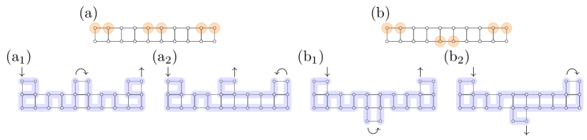
Figure 11: (a) $(3,0)$-vertex gadget and (b) $(2,1)$-vertex gadget, with highlighted outlets. (a₁), (a₂) and (b₁), (b₂) show two generic ways a Hamiltonian cycle can pass through each vertex gadget.

We will refer to the outlets as top or bottom outlets, as well as the left, middle or right outlet, with the obvious meaning. The left and right outlets are also called the outer outlets.

We will now define the gadget expansion of a 3-regular graph $G$, consisting of a graph $G^{\prime}$ and a straight-line embedding $\operatorname{emb}$ resulting from applying the following steps to $G$.

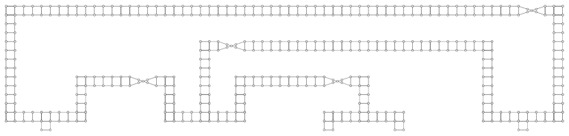
Figure 12: Gadget expansion of the graph pictured in Fig. 2. This graph is not 3-regular, but we may assume that there are further edges in $E_{2}$.

Construction 3 (Gadget expansion).

Start with $G^{\prime}$ being the empty graph (see Fig. 12 for an illustration).

Step 1: Compute a 2-page book embedding of $G$ and let $v_{1},\ldots,v_{n}$ be the vertices of $G$ in the order in which they appear on the spine, and let $\{E_{1},E_{2}\}$ denote the partition of $E$.

Step 2: For every vertex $v_{i}\in V$ add to $G^{\prime}$ a $(\deg_{1}(v_{i}),\deg_{2}(v_{i}))$-vertex gadget. Position the vertices of this gadget at $(18i+x,y)$ with $x\in\{0,\ldots,9\}$ and $y\in\{0,1\}$, as in Fig. 11.

Step 3: For every edge $e=\{v_{i},v_{j}\}$ in $E_{1}$, $i<j$, add to $G^{\prime}$ a ladder path $L_{k_{1},k_{2}}$ connected to an outlet in $v_{i}$’s vertex gadget and an outlet in $v_{j}$’s vertex gadget as follows. Recall the ordering of the edges incident to a vertex defined in the preliminaries. If $e$ is the $r$-th edge at $v_{i}$ and the $s$-th edge at $v_{j}$, then attach said ladder path to the $r$-th top outlet from the left of $v_{i}$’s vertex gadget and to the $s$-th top outlet from the left of $v_{j}$’s vertex gadget. If only one of these two outlets is an outer outlet, then attach the end of the first half to that outlet and the end of the second half to the other (middle) outlet. (If the outlets are both outer or both middle outlets, then it does not matter which end of the ladder path is connected to which outlet.) This is done by adding two disjoint edges which connect the two vertices forming an end of the ladder path to the two vertices forming the corresponding outlet as in Fig. 12.

The value of $k_{1}$ is chosen as $k_{1}\coloneqq 6h(e)$ and the value of $k_{2}$ as follows. Define $\alpha$ to be $0,4$ or $8$, if the ladder path is attached to the left, middle or right outlet of $v_{i}$’s vertex gadget, respectively. Define $\beta$ in the same manner for $v_{j}$. Set $k_{2}\coloneqq 18(j-i)-\alpha+\beta-5$. Note that $k_{2}\geq 5$ always holds. Finally, we will give the embedding of the ladder path’s vertices, using the designations introduced in the definition of a ladder path. We only state the case where the first half is attached to $v_{i}$, for the other case the coordinates are to be mirrored at a suitable vertical axis. The positions of the vertices in the first half are (with $S_{i}^{\alpha}\coloneqq 18i+\alpha$):

$$\operatorname{emb}(u_{r}^{1}) \coloneqq(S_{i}^{\alpha},r+2), \operatorname{emb}(\tilde{u}_{r}^{1}) \coloneqq(S_{i}^{\alpha}+1,r+2),\quad\,r=0,\ldots,k_{1}-1$$

$$\operatorname{emb}(u_{r}^{2}) \coloneqq(S_{i}^{\alpha}+2+r,k_{1}+1), \operatorname{emb}(\tilde{u}_{r}^{2}) \coloneqq(S_{i}^{\alpha}+2+r,k_{1}),\quad r=0,\ldots,k_{2}-1$$

$$\operatorname{emb}(w_{1}) \coloneqq(S_{i}^{\alpha}+k_{2}+2,k_{1}+2/3), \operatorname{emb}(w_{2}) \coloneqq(S_{i}^{\alpha}+k_{2}+2,k_{1}+1/3),$$

$$\operatorname{emb}(w_{3}) \coloneqq(S_{i}^{\alpha}+k_{2}+2.5,k_{1}+1/2), \operatorname{emb}(w_{4}) \coloneqq(S_{i}^{\alpha}+k_{2}+3,k_{1}+2/3),$$

$$\operatorname{emb}(w_{5}) \coloneqq(S_{i}^{\alpha}+k_{2}+3,k_{1}+1/3), \operatorname{emb}(w_{6}) \coloneqq(S_{i}^{\alpha}+k_{2}+4,k_{1}+1),$$

$$\operatorname{emb}(w_{7}) \coloneqq(S_{i}^{\alpha}+k_{2}+4,k_{1}).$$

Compare Fig. 10. The positions of the vertices in the second half are analogous to the first.

Step 3 must be repeated for $E_{2}$ using negative $y$-coordinates. $\diamond$

This construction is useful due to the following:

Lemma 7.

Gadget expansion preserves Hamiltonicity.

Proof.

First, assume that $G^{\prime}$ contains a Hamiltonian cycle $C^{\prime}$. By Lemma 6, $C^{\prime}$ contains either a traversal or a partial and a full cover of each ladder path. We obtain a Hamiltonian cycle in $G$ by including each edge $e$ if and only if $C^{\prime}$ contains a traversal of the ladder path representing $e$.

Conversely, assume that $G$ contains a Hamiltonian cycle $C$. We construct a Hamiltonian cycle $C^{\prime}$ in $G^{\prime}$ by including a traversal of each ladder path representing an edge contained in $C$ as well as a full cover of one half of each ladder path representing an edge not contained in $C$ and a partial cover of the other half. We additionally add several edges in the vertex gadgets to $C^{\prime}$. Which edges we pick depends on the type of the vertex gadget and which of the attached ladder paths are traversed and which are covered. There are four main cases (note that at each gadget there must be exactly two traversed ladder paths):

• a $(3,0)$-vertex gadget with both outer ladder paths traversed;

• a $(3,0)$-vertex gadget with the middle and one outer ladder path traversed;

• a $(2,1)$-vertex gadget with both outer ladder paths traversed;

• a $(2,1)$-vertex gadget with the middle and one outer ladder path traversed.

Other cases are symmetric to one of these four. In each case, the edges included in $C^{\prime}$ are highlighted in Fig. 11. ∎

5.2 Face Filling

In order to turn the gadget expansion of a graph into an RNG and GG, we need to add buffers. The challenge is doing this in a way that preserves Hamiltonicity. We call an edge $e$ of $G$ permissible if $G$ is not Hamiltonian or if $G$ contains a Hamiltonian cycle that passes through $e$.

Lemma 8.

Subdividing a permissible edge preserves Hamiltonicity. Moreover, both edges resulting from the subdivision are permissible in the resulting graph.

Proof.

Let $e$ be a permissible edge of $G$ and $G^{\prime}$ be obtained from $G$ by subdividing $e$. If $G$ is not Hamiltonion, then clearly $G^{\prime}$ is neither. Otherwise, if the edge $e$ is contained in a Hamiltonian cycle $C$, then $C$ induces a Hamiltonian cycle $C^{\prime}$ in $G^{\prime}$ which contains the two edges created by the subdivision. ∎

Figure 13: An example of a permissible cycle addition with a cycle of length 12.

Our main tool for adding buffers to a graph is called permissible cycle addition. Let $\{u_{1},u_{2}\}$ be a permissible edge of $G=(V,E)$. We say that $G^{\prime}=(V^{\prime},E^{\prime})$ is obtained from $G$ by attaching a permissible cycle to $\{u_{1},u_{2}\}$ if (see Fig. 13 for an illustration)

• $V^{\prime}=V\uplus\{v_{1},\ldots,v_{k}\}$, $k\geq 4$, and $v_{1},\ldots,v_{k}$ induce a cycle in that order, that is, $\{v_{i},v_{j}\}\in E^{\prime}$ if and only if $|i-j|=1$ or $\{i,j\}=\{1,k\}$;

• $E^{\prime}\cap\binom{V}{2}=E$;

• for all $i\in\{2,\ldots,k-1\}$, if $\deg_{G^{\prime}}(v_{i})\geq 3$, then $\deg_{G^{\prime}}(v_{i-1})=\deg_{G^{\prime}}(v_{i+1})=2$; and

• $\deg_{G^{\prime}}(v_{1})=\deg_{G^{\prime}}(v_{k})=3$, and $\{\{v_{1},u_{1}\},\{v_{k},u_{2}\}\}\subseteq E^{\prime}$.

Fig. 13 pictures an example of such a cycle addition. This modification is useful due to:

Lemma 9.

Permissible cycle addition preserves Hamiltonicity. Moreover, if $v_{1},\ldots,v_{k}$ is the added cycle, then the edges $\{v_{i},v_{i+1}\}$, $1\leq i<k$, are all permissible in the resulting graph.

Proof.

Suppose that $G^{\prime}=(V^{\prime},E^{\prime})$ is obtained by permissible cycle addition from $G=(V,E)$ with $v_{1},\ldots,v_{k}$ being the cycle added and $\{u_{1},u_{2}\}$ the permissible edge in $G$ to which it is attached.

First, suppose that $G^{\prime}$ contains a Hamiltonian cycle. Due to Lemma 5, this cycle cannot pass through any edge $\{w,v_{i}\}$, $w\in V\setminus\{u_{1},u_{2}\}$. Hence, it must pass through $u_{1},v_{1},\ldots,v_{k},u_{2}$ in that order or in reversed order. Thus, all edges on the cycle except for possibly $\{v_{1},v_{k}\}$ are permissible. Removing $v_{1},\ldots,v_{k}$ from this cycle and adding the edge $\{u_{1},u_{2}\}$ yields a Hamiltonian cycle in $G$.

Conversely, suppose that $G$ contains a Hamiltonian cycle. Because edge $\{u_{1},u_{2}\}$ is permissible, $G$ contains a Hamiltonian cycle that passes through $\{u_{1},u_{2}\}$. By inserting $v_{1},\ldots,v_{k}$ between $u_{1}$ and $u_{2}$ we obtain a Hamiltonian cycle in $G^{\prime}$. ∎

In order to be able to apply permissible cycle addition to the gadget expansion $G^{\prime}$ of a graph $G$, we need to know permissible edges of $G^{\prime}$. For this, we have the following lemma.

Lemma 10.

Let $G$ be a 3-regular graph, $G^{\prime}$ the gadget expansion of $G$, and $L$ any ladder path of $G^{\prime}$ whose first half is attached to an outer outlet (of a vertex gadget). Then, $L$ contains two even inside and two even outside edges, all of which are permissible. Furthermore, these edges can be determined in linear time.

Proof.

We give the proof for the outside edges, for the inside edges everything works analogously. Write $L=L_{k_{1},k_{2}}$. By construction of the gadget expansion, we have $k_{1}\geq 6$ and $k_{2}\geq 4$. Thus, using the vertex names from the definition of a ladder path, the edges $\{u^{1}_{0},u^{2}_{1}\},\{u^{1}_{2},u^{1}_{3}\},\{u^{2}_{0},u^{2}_{1}\}$, and $\{u^{2}_{2},u^{2}_{3}\}$ are even outside edges.

It remains to show that at least two of these are permissible. So assume that $G^{\prime}$ (and thus $G$) is Hamiltonian (otherwise we are done) and let $C$ be a Hamiltonian cycle of $G$ and $C^{\prime}$ the corresponding Hamiltonian cycle of $G^{\prime}$ as given by Lemma 7. By Lemma 6, $L$ is either covered or traversed by $C^{\prime}$. If it is covered, then $C^{\prime}$ contains every inside and outside edge of $L$. If it is traversed, then the case analysis in Fig. 11 reveals that $C^{\prime}$ contains either $\{u^{1}_{0},u^{2}_{1}\}$ or $\{\tilde{u}^{1}_{0},\tilde{u}^{1}_{1}\}$ (which one depends on the type of the vertex gadget). In former case, $C^{\prime}$ also contains $\{u^{1}_{2},u^{1}_{3}\}$. In the latter case, $C^{\prime}$ contains $\{u^{2}_{0},u^{2}_{1}\}$ and $\{u^{2}_{2},u^{2}_{3}\}$ (cf. Fig. 10.(b)). This proves the claim. Note that determining the two permissible edges does not require knowledge of $C^{\prime}$ but only of the vertex gadget type. ∎

We are set to give the construction in our polynomial-time many-one reduction from HC on $3$-regular planar graphs to HC on RNGs or GGs.

Construction 4.

Let $G=(V,E)$ be a $3$-regular planar graph. We will construct an RNG and GG $G^{\prime}=(V^{\prime},E^{\prime})$ that is Hamiltonian if and only if $G^{\prime}$ is. We will give the embedding of the vertices directly in the reduction.

We start with ($G^{\prime}$, $\operatorname{emb}$), the gadget expansion of $G$. We add one buffer for every $(x,y)\in\mathbb{Z}^{2}$ where $14\leq x\leq 16n+10$ and $-6h_{2}(G)-2\leq y\leq 6h_{1}(G)+2$ are both even, except when $G^{\prime}$ already contains a vertex $v$ with $\operatorname{emb}(v)\in\{(x,y),(x+1,y)\}$. The buffer then consists of a 4-cycle whose vertices are embedded at $(x,y),(x+1,y),(x+1,y+1)$, and $(x,y+1)$ and whose edges are then further subdivided. We call it the $(x,y)$-buffer and refer to the four (subdivided) edges as its sides. For each side, if $G^{\prime}$ previously already contained a (possibly subdivided) edge running parallel to that side at distance 1, then we say that this side adjoins that (possibly subdivided) edge. For example, the side from $(x,y+1)$ to $(x+1,y+1)$ would adjoin an existing edge from $(x,y+2)$ to $(x+1,y+2)$. A side may also adjoin an edge in a switch to which it is not parallel. For example, the side from $(x,y+1)$ to $(x+1,y+1)$ could adjoin an existing edge from $(x,y+2)$ to $(x+1,y+2+1/3)$. Finally, exactly one of the four sides will be designated as the docking side. The docking side must adjoin either a side of a previously added buffer or a permissible edge of the gadget expansion.

When adding a buffer, if its sides adjoin existing sides or edges, then we also add edges connecting the buffer to other vertices and possibly also subdivide the adjoined edges or sides. There are four cases, depending on whether the newly added side is docking or non-docking and whether it adjoins a side of another buffer or an edge of the gadget expansion. These four cases are illustrated in Fig. 14. In particular,

• the docking side of the added buffer is always subdivided four times and has four edges connecting it to the side or edge it adjoins (see Fig. 14(a) and (b));

• a non-docking side adjoining an edge of the gadget expansion is subdivided once and has two connecting edges (see Fig. 14(c));

• a non-docking side adjoining another buffer’s side is subdivided thrice and has three connecting edges (see Fig. 14(d));

• a (non-docking) side which does not adjoin anything, then it is only subdivided once.

Figure 14: Construction of the sides of a cycle (left) with (a) a docking side adjoined to an edge, (b) a docking side adjoined to a previously existing non-docking side, (c) a non-docking side adjoined to an edge, and (d) a non-docking side adjoined to an existing side. In each picture, an edge or previously existing side to adjoin is on the right. The vertices and edges that result from the addition of the cycle are marked in blue while previously existing vertices and edges are in black.

Fig. 14 explains the positions of the sides’ subdivisions by way of an example for the right-side case. For the case of the other three sides, the coordinates are obtained by rotating around $(x+1/2,y+1/2)$.

The docking side must adjoin another buffer’s side or a permissible edge. We will now discuss a strategy to achieve this. First, observe that every position $(x,y)$ at which we intend to add a buffer lies in a face of $(G^{\prime},\operatorname{emb})$ that borders more than four vertices (possibly the unbounded face). We call these faces the regions and will add the buffers region-by-region. Next, note that once a buffer has been added to a region, then any subsequent buffer in that region can have its docking side adjoined to a (non-docking) side of another buffer added before it, as all edges on non-docking sides of a buffer are permissible by Lemma 9. (The gadget expansion is “surrounded” with buffers, so this works for the unbounded face.) Thus, it suffices to show how to add the first buffer for each region.

To this end, we must examine the structure of the gadget expansion. Let $R$ be any region. Clearly, $R$ borders some vertex gadget, and thus also a ladder path $L$ attached to an outside outlet of that vertex gadget. More precisely, $R$ borders either every inside or every outside edge of $L$. By construction of the gadget expansion, the first half of $L$ is attached to an outside outlet of some vertex gadget. Thus, we can find two permissible edges of $L$ that border $R$ by Lemma 10. Because we have two permissible edges to choose from, we can ensure that we never adjoin the docking sides of two buffers to two “parallel” edges of $L$ (i.e., to $\{u^{j}_{i},u^{j}_{i+1}\}$ and $\{\tilde{u}^{j}_{i},\tilde{u}^{j}_{i+1}\}$), as every ladder path only borders two regions. $\diamond$

We are now prepared to prove the main result of this section.

Proof of Theorem 4.

The proof builds on Construction 4. By Lemma 7, gadget expansion preserves Hamiltonicity. Each addition of a cycle involves subdividing a permissible edge (preserving Hamiltonicity by Lemma 8), and then adding a permissible cycle (preserving Hamiltonicity by Lemma 9). It follows that the construction preserves Hamiltonicity.

The construction already describes an embedding of the resulting graph $G^{\prime}$. So it only remains to show that this embedding induces $G^{\prime}$ as its RNG and GG. Let $\mathcal{A}\coloneqq\{(x,y)\in\mathbb{Z}^{2}\mid 14\leq x\leq 16n+11,\,-6h_{2}(G)-2\leq y\leq 6h_{1}(G)+3\}$. Note that for most $(x,y)\in\mathcal{A}$ there is a vertex embedded at $(x,y)$. The only exceptions are positions surrounding switches. For any $(x,y)\in\mathcal{A}$ we will call the vertices embedded at $(x,y)$, $(x+1,y)$, $(x,y+1)$, and $(x+1,y+1)$ along with any vertices embedded on the line segments between those four points a grid face. There are three classes of grid faces: grid faces within ladder paths or vertex gadgets, buffers, and grid faces between the aforementioned ones.

Within ladder paths, only two grid faces, which are shown in Fig. 15 ($A$ and $B$), can occur. For these, it is easy to see that all nonadjacent vertex pairs have a GG blocker. Within buffers, more variations are possible (e.g. $C$ and $D$ in Fig. 15). However, the vertices in the corners and in the center of each side serve as GG blockers for all nonadjacent pairs. All grid faces between cycles or between cycles and vertex gadgets are pictured in Fig. 14. Again, it is easy to see that all pairs of non-adjacent vertices have GG blockers and no pair of adjacent vertices has an RNG blocker.

Figure 15: An excerpt of the graph $G^{\prime}$ produced by the reduction: Grid faces in $G^{\prime}$: (A) Grid face within a ladder path or a vertex gadget with no docking side adjoined to its edges. (B) Grid face within a ladder path or a vertex gadget with a docking side adjoined to one of its edges. (C) + (D) Grid faces within buffers with the docking side on the right.

We now consider the area surrounding a switch. This area is pictured in Fig. 15. The vertex $e$ is not a GG blocker for $\{a,b\}$, because $\operatorname{d}(a,b)^{2}=1/9$ and $\operatorname{d}(a,e)^{2}=\operatorname{d}(b,e)^{2}=5/18$. The vertex marked $d$ is also not a GG blocker for $\{b,c\}$, since $\operatorname{d}(b,c)^{2}=16/9$, $\operatorname{d}(b,d)^{2}=10/9$, and $\operatorname{d}(c,d)^{2}=2$. Other cases are analogous or easy to see. Vertices that do not share a grid face are not adjacent by Lemma 1.

If $n$ is the number of vertices in the input graph $G$, then the graph $G^{\prime}$ output by the construction contains $n$ vertex gadgets each containing $\mathcal{O}(1)$ vertices, $\mathcal{O}(n)$ ladder paths with $\mathcal{O}(n)$ vertices, and $\mathcal{O}(n^{2})$ cycles with $\mathcal{O}(1)$ vertices. It is easy to see that each step in both constructions can be computed in polynomial time. Along with Proposition 1, this implies that HC is $\operatorname{NP}$-hard on RNGs and on GGs. Moreover, it also implies that HC cannot be decided by a $2^{o(n^{1/4})}$-time algorithm on RNGs or GGs, unless the ETH fails. ∎

The computational complexity of Hamiltonian Cycle on RCGs and that of HC on RNGs and GGs with maximum degree three is left open.

6 Independent Set

In this section, we will investigate the restriction of the following problem to RNGs, RCGs, and Gabriel graphs:

Problem 5.

Independent Set (IS)

Input: An undirected graph $G=(V,E)$ and $k\in\mathbb{N}_{0}$.

Question: Is there a vertex set $X\subseteq V$ with $|X|\geq k$ such that $G[X]$ is edgeless?

We will show:

Theorem 5.

Independent Set on RCGs, on RNGs, and on GGs is $\operatorname{NP}$-hard, even if the maximum degree is four. Moreover, unless the ETH fails, it admits no $2^{o(n^{1/4})}$-time algorithm where $n$ is the number of vertices.

Our proof is based on a polynomial-time many-one reduction from the $\operatorname{NP}$-hard [24] Independent Set on planar graphs with maximum degree three.

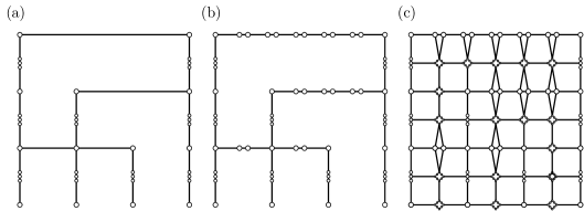
Figure 16: Construction 5 applied to the example graph in Fig. 2. (a) The graph after steps 1–2. (b) The graph after steps 1–3. (c) The final graph.

Construction 5.

Let $G=(V,E)$ be a planar graph with maximum degree three and let $k\in\mathbb{N}_{0}$. We construct a graph $G^{\prime}=(V^{\prime},E^{\prime})$’ and $k^{\prime}\in\mathbb{N}_{0}$ such that $G^{\prime}$ is an RNG and a GG (we will discuss RCGs later), and $G$ contains an independent set of size $k$ if and only if $G^{\prime}$ contains one of size $k^{\prime}$ (see Fig. 16 for an illustration).

We start with $G^{\prime}\coloneqq G$ and $k^{\prime}\coloneqq k$.

Step 1: Compute a 2-page book embedding of $G$ and let $v_{1},\ldots,v_{n}$ be the vertices of $G$ enumerated in the order in which they appear on the spine, and let $\{E_{1},E_{2}\}$ denote the partition of $E$.

Step 2: Replace every vertex $v_{i}\in V$ with a path consisting of $4h_{1}(v_{i})+4h_{2}(v_{i})+1$ vertices $w_{-4h_{2}(v_{i})},\ldots,w_{4h_{1}(v_{i})}$ and increase $k^{\prime}$ by $2h_{1}(v_{i})+2h_{2}(v_{i})$. For $j=-h_{2}(v_{i}),\ldots,h_{1}(v_{i})$, the vertex $w_{4j}$ forms the $(2i,2j)$-corner. For $j=-h_{2}(v_{i}),\ldots,h_{1}(v_{i})-1$, the vertices $w_{4j+1},w_{4j+2},w_{4j+3}$ jointly form the $(2i,2j+1)$-corner, with $w_{4j+2}$ being both the left and right connecting vertex.

Every edge $e$ of $G$ incident to $v_{i}$ is now instead attached to $w_{4h(e)}$ (if $e\in E_{1}$) or $w_{-4h(e)}$ (if $e\in E_{2}$).

Step 3: For every edge $e=\{v_{i},v_{j}\}\in E_{1}$, $i<j$, subdivide the corresponding edge of $G^{\prime}$ a total of $4\ell(e)-2$ times and increase $k^{\prime}$ by $2\ell(e)-1$. Suppose that $w_{1},\ldots,w_{4\ell(e)-2}$ are the vertices introduced in the subdivision. For every $x\in\{1,\ldots,2\ell-1\}$, the vertices $w_{2x-1}$ and $w_{2x}$ jointly form the $(2i+x,2h(e))$-corner, with each being both top and bottom connecting vertex.

Repeat this step for $E_{2}$ using negative $y$-coordinates instead.

Step 4: For every $(x,y)\in\mathbb{Z}^{2}$ with $2\leq x\leq 2n$ and $-4h_{2}(G)\leq y\leq 4h_{1}(G)$, if no $(x,y)$-corner was added in any of the previous steps, then add a copy of $C_{8}$, call it the $(x,y)$-corner, and increase $k^{\prime}$ by $4$. The first, third, fifth, and seventh vertex on the cycle are the top, left, bottom, and right connecting vertex of that corner, respectively. Make the top connecting vertex of the $(x,y)$-corner adjacent with the bottom connecting vertices of the $(x,y+1)$-corner, the left connecting vertex of the $(x,y)$-corner adjacent with the right connecting vertices of the $(x-1,y)$-corner, and so on. $\diamond$

Lemma 11.

Let $G=(V,E)$ and $G^{\prime}=(V^{\prime},E^{\prime})$ be graphs and let $\alpha(G)$ and $\alpha(G^{\prime})$ denote the size of a largest independent set in each graph.

1. If $G^{\prime}$ is obtained from $G$ by replacing a vertex $v\in V$ with a path consisting of $2k+1$ new vertices $v_{1},\ldots,v_{2k+1}$ in that order and connecting each $u\in N_{G}(v)$ to an arbitrary vertex in $\{v_{2i+1}\mid 0\leq i\leq k\}$, then $\alpha(G^{\prime})=\alpha(G)+k$.

2. If $G^{\prime}$ is obtained from $G$ by subdividing an edge $e\in E$ a total of $2k$ times, then $\alpha(G^{\prime})=\alpha(G)+k$.

3. If $G^{\prime}$ is obtained from $G$ by adding a copy of the cycle $C_{8}$ such that no two consecutive vertices in the cycle have a neighbor outside of the cycle, then $\alpha(G^{\prime})=\alpha(G)+4$.

4. If $G^{\prime}$ is obtained from $G$ using Construction 5 and $n$ is the number of vertices in $G$, then $G^{\prime}$ contains at most $\mathcal{O}(n^{2})$ vertices.

Proof.

1. Define $V_{\textnormal{odd}}:=\{v_{2i+1}\mid 0\leq i\leq k\}$ and $V_{\textnormal{even}}:=\{v_{2i}\mid 1\leq i\leq k\}$.

   Let $X\subseteq V$ be an independent set in $G$. If $v\in X$, then $(X\setminus\{v\})\cup V_{\textnormal{odd}}$ is an independent set of size $|X|+k$ in $G^{\prime}$. If $v\notin X$, then $X\cup V_{\textnormal{even}}$ is an independent set of that size. Conversely, let $X^{\prime}\subseteq V^{\prime}$ be an independent set in $G^{\prime}$. Note that $\lvert X^{\prime}\cap\{v_{1},\dots,v_{2k+1}\}\rvert\leq k+1$ with equality if and only if $V_{\textnormal{odd}}\subseteq X^{\prime}$. If $V_{\textnormal{odd}}\subseteq X^{\prime}$, then $(X^{\prime}\setminus V_{\textnormal{odd}})\cup\{v\}$ is an independent set of $G$ of size $\lvert X^{\prime}\rvert-k$. Otherwise, $X^{\prime}\setminus\{v_{1},\dots,v_{2k+1}\}$ is an independent set of $G$ of size at least $\lvert X^{\prime}\rvert-k$.

2. Follows from (i).

3. Let $X\subseteq V$ be an independent set in $G$. The added copy of $C_{8}$ contains at least four pairwise non-adjacent vertices without any neighbors in $G$. Adding these four vertices to $X$ yields an independent set in $G^{\prime}$ of size $|X|+4$. Conversely, let $X^{\prime}\subseteq V^{\prime}$ be an independent set in $G^{\prime}$. Since $X^{\prime}$ can contain at most four vertices from the copy of $C_{8}$, removing any such vertices yields an independent set in $G$ of size at least $|X^{\prime}|-4$.

4. The graph $G^{\prime}$ contains $\mathcal{O}(n^{2})$ corners each containing $\mathcal{O}(1)$ vertices.

∎

We are now ready to prove the main result of this section:

Proof of Theorem 5.

The correctness of steps 2 to 4 follows from Lemma 11(i) to (iii), respectively. By Lemma 11(iv), the size of the output graph of the reduction is polynomial in the size of the input graph and it is easy to see that the computations in the construction may be carried out in polynomial time. The degree restriction follows from the fact that the reduction does not generate any vertices with degree greater than $4$.

We will now argue that the graph $G^{\prime}$ output by Construction 5 is an RNG and a GG. We begin by giving an embedding of the graph. If the $(x,y)$-corner is a single vertex, then its embedding is $(x,y)$. If the $(x,y)$-corner consists of three vertices added in step 2, then they are embedded at $(x,y-\varepsilon)$, $(x,y)$, and $(x,y+\varepsilon)$. If the $(x,y)$-corner consists of two vertices added in step 3, then their positions are $(x\pm\varepsilon,y)$. Finally, if the $(x,y)$-corner is a copy of $C_{8}$, then the vertices in this cycle are embedded at $(x\pm\varepsilon,y),(x\pm\frac{\varepsilon}{2},y\pm\frac{\varepsilon}{2}),(x,y\pm\varepsilon)$.

We must show that this embedding induces $G^{\prime}$ as its RNG and as its GG.

For any $(x,y)\in\mathbb{Z}^{2}$ with $2\leq x<2n$ and $-4h_{2}(G)\leq y<4h_{1}(G)$, the $(x,y)$-grid face is the set of all vertices contained in the corners $(x,y)$, $(x+1,y)$, $(x,y+1)$, and $(x+1,y+1)$. By Lemma 1, vertices that do not share a grid face are non-adjacent in the GG induced by the embedding, implying that they are also non-adjacent in the RNG. It remains to show that there is a GG blocker for each pair of non-adjacent vertices that do share a grid face, but no RNG blocker for any edge. Fig. 17 pictures all types of grid faces that may occur in $G^{\prime}$ (up to symmetry).

Figure 17: Grid faces created by Construction 5.

In most cases, the claim is obvious. We consider the face pictured in Fig. 17(a). The vertex labeled $b$ is a GG for $\{a,c\}$, because $\operatorname{d}(a,c)^{2}=1$, $\operatorname{d}(a,b)^{2}=2\varepsilon^{2}$, and $\operatorname{d}(b,c)^{2}=(1-\varepsilon)^{2}+\varepsilon^{2}$ implies that for sufficiently small $\varepsilon$ (i.e., $\varepsilon\leq(\sqrt{5}-1)/4$) we get $\operatorname{d}(a,c)^{2}-\operatorname{d}(a,b)^{2}-\operatorname{d}(b,c)^{2}=1-2\varepsilon-4\varepsilon^{2}\geq 0$.

Similarly, $a$ is a GG blocker for $\{d,e\}$, since

$$\operatorname{d}(d,e)^{2}=(1-\varepsilon)^{2},\quad\operatorname{d}(d,a)^{2}=\frac{\varepsilon^{2}}{2},\quad\text{and}\quad\operatorname{d}(a,e)^{2}=\left(1-\frac{3\varepsilon}{2}\right)^{2}+\frac{\varepsilon^{2}}{4}$$

implies that for sufficiently small $\varepsilon$ (i.e., $\varepsilon\leq 1/2$)

$$\operatorname{d}(d,e)^{2}-\operatorname{d}(d,a)^{2}-\operatorname{d}(a,e)^{2}=\varepsilon-2\varepsilon^{2}\geq 0.$$

The other cases are either obvious or follow along the same lines as these two.

Relatively closest graphs. In the RCG induced by the embedding described above, the edges highlighted in Fig. 17(d)–(f), which connect a $C_{8}$ to a corner added in step 3, do not exist. This is not an issue, however, since the proof of the correctness of the reduction does not rely on the existence of those edges. Hence, an adjusted reduction that omits these edges proves the $\operatorname{NP}$-hardness of the problem on RCGs.

ETH-based lower bound. By Lemma 2, Vertex Cover does not admit a $2^{o(n^{1/2})}$-time algorithm on planar graphs with maximum degree three where $n$ is the number of vertices unless the ETH fails, and neither does Independent Set. By Lemma 11(iv), the reduction only increases the number of vertices quadratically. Thus, IS on RCGs, RNGs, and GGs does not admit a $2^{o(n^{1/4})}$ time algorithm unless the ETH fails. ∎

7 Dominating Set

In this section, we will investigate the restriction of the following problem to RNGs, RCGs, and Gabriel graphs:

Problem 6.

Dominating Set (DS)

Input: An undirected graph $G=(V,E)$ and $k\in\mathbb{N}_{0}$.

Question: Is there a vertex set $X\subseteq V$ with $|X|\leq k$ such that $N_{G}[X]=V$?

We will show:

Theorem 6.

Dominating Set on RCGs, on RNGs, and on GGs is $\operatorname{NP}$-hard, even if the maximum degree is four, Moreover, unless the ETH fails, it admits no $2^{o(n^{1/4})}$-time algorithm where $n$ is the number of vertices.

Dominating Set on $3$-regular planar graphs is claimed [27, 32] to be $\operatorname{NP}$-hard, but we do not know of a published full proof. We give a proof sketch for the following related statement:

Lemma 12.

Dominating Set on planar graphs with maximum degree three is $\operatorname{NP}$-hard and, unless the ETH fails, admits no $2^{o(n^{1/2})}$-time algorithm where $n$ is the number of vertices.

Proof.

By Lemma 2, the Vertex Cover problem on planar graphs with maximum degree three does not admit a $2^{o(n^{1/2})}$-time algorithm where $n$ is the number of vertices, unless the ETH fails. Vertex Cover on planar graphs with maximum degree three can be reduced to Dominating Set on planar graphs with maximum degree six using a standard reduction that involves deleting isolated vertices and replacing every edge with a $3$-cycle. This reduction only changes the size of the graph linearly. Hence, the same claim applies to Dominating Set on planar graphs with maximum degree six. The vertex expansion operation employed by Chen et al. [13, Sect. 3.2] in a similar context may be used to reduce the maximum degree to three while also only changing the size of the graph linearly. Hence, unless the ETH fails, Dominating Set cannot be solved in time $2^{o(n^{1/2})}$ on planar graphs with maximum degree three. where $n$ is the number of vertices. ∎

We will now present the construction of a polynomial-time many-one reduction from DS on planar graphs with maximum degree three to DS restricted to graphs that are RCGs, RNGs, and GGs.

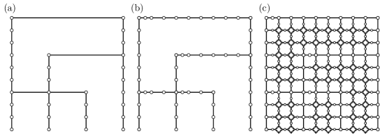
Figure 18: Construction 6 applied to the example graph in Fig. 2. (a) The graph after steps 1–2. (b) The graph after steps 1–3. (c) The final graph.

Construction 6.

Let $G=(V,E)$ be a planar graph with maximum degree three and let $k\in\mathbb{N}_{0}$. We will construct a graph $G^{\prime}=(V^{\prime},E^{\prime})$ and $k^{\prime}\in\mathbb{N}_{0}$ such that $G^{\prime}$ is an RCG, an RNG, and a GG, and $G$ contains a dominating set of size $k$ if and only if $G^{\prime}$ contains one of size $k^{\prime}$ (see Fig. 18 for an illustration).

The vertex set $V^{\prime}$ will mostly consist of groups of vertices called $(x,y)$-corners, where $3\leq x\leq 3n$ and $-3h_{2}(G)\leq y\leq 3h_{1}(G)$. Each corner consists of either a single vertex or a copy of the cycle $C_{12}$. In the RNG-embedding of $G^{\prime}$, the vertices forming the $(x,y)$-corner will be embedded roughly around the coordinate $(x,y)$. If $u_{1},\ldots,u_{12}$ are the vertices in a copy of $C_{12}$ in the order in which they appear on the cycle, then we refer to $u_{1},u_{4},u_{7},u_{10}$ as the top, right, bottom, and left connecting vertices. The connecting vertices will be the only vertices in a copy of $C_{12}$ with neighbors outside of that cycle. If a corner consists of a single vertex, then that vertex itself simultaneously forms the top, bottom, left, and right connecting vertex of that corner. We start with $G^{\prime}\coloneqq G$ and $k^{\prime}\coloneqq k$.

Step 1: Compute a 2-page book embedding of $G$. Let $v_{1},\ldots,v_{n}$ be the vertices of $G$ enumerated in the order in which they appear on the spine, and let $\{E_{1},E_{2}\}$ denote the partition of $E$.

Step 2: Replace each vertex $v_{i}$ with a path of length $3h_{1}(v_{i})+3h_{2}(v_{i})$. The vertices on this paths form the corners $(3i,-3h_{2}(v_{i})),(3i,-3h_{2}(v_{i})+1),\dots,(3i,3h_{1}(v_{i}))$. Every edge $e$ of $G$ incident to $v_{i}$ is now instead attached to the $(3i,3h(e))$-corner if $e\in E_{1}$ or the $(3i,-3h(e))$-corner if $e\in E_{2}$. Increase $k^{\prime}$ by $h_{1}(v_{i})+h_{2}(v_{i})$.

Step 3: For every edge $e=\{v_{i},v_{j}\}\in E_{1}$, subdivide the corresponding edge in $G^{\prime}$ a total of $3\ell(e)$ times and increase $k^{\prime}$ by $\ell(e)$. Suppose that $w_{0},\ldots,w_{3\ell(e)-1}$ are the vertices introduced in the subdivision, where $w_{0}$ is adjacent with the $(3i,3h(e))$-corner. Then, $w_{0}$ is not a corner, but for every $x\in\{1,\ldots,3\ell(e)-1\}$, $w_{x}$ is the $(3i+x,3h(e))$-corner.

Step 4: For every $(x,y)$ with $3\leq x\leq 3n$ and $0\leq y\leq 3h_{1}(G)$, if an $(x,y)$-corner was not added in the previous two steps, then add a copy of $C_{12}$ and call it the $(x,y)$-corner. Then add an edge connecting the top connecting vertex of the $(x,y)$-corner with the bottom connecting vertex of the $(x,y+1)$-corner, the left connecting vertex of the $(x,y)$ corner with the right connecting vertex of the $(x-1,y)$-corner, and so on. Subdivide each of these edges once.

Steps 2 to 4, take only $E_{1}$ into account. These steps must be repeated analogously for the edges in $E_{2}$ using negative $y$-coordinates. $\diamond$

Lemma 13.

Let $G=(V,E)$ and $G^{\prime}$ be graphs and let $\gamma(G)$ and $\gamma(G^{\prime})$ denote the size of a smallest dominating set in each graph. Let $k\in\mathbb{N}_{0}$.

1. If $G^{\prime}$ is obtained from $G$ by replacing a vertex $v\in V$ with a path consisting of $3k+1$ new vertices $v_{1},\ldots,v_{3k+1}$ in that order and connecting each $u\in N_{G}(v)$ to an arbitrary vertex in $\{v_{3i+1}\mid 0\leq i\leq k\}$, then $\gamma(G^{\prime})=\gamma(G)+k$.

2. If $G^{\prime}$ is obtained from $G$ by subdividing an edge $e\in E$ a total of $3k$ times, then $\gamma(G^{\prime})=\gamma(G)+k$.

3. If $G^{\prime}$ is obtained from $G$ by adding a copy of the cycle $C_{12}$ and connecting a subset of its connecting vertices each to at most one existing vertex via a path of length two, then $\gamma(G^{\prime})=\gamma(G)+4$.

4. If $G^{\prime}$ is obtained from $G$ using Construction 6 and $n$ is the number of vertices in $G$, then $G^{\prime}$ contains at most $\mathcal{O}(n^{2})$ vertices.

Proof.

1. It suffices to prove the claim for $k=1$. The general case then follows by induction.

   Suppose that $X\subseteq V$ is a dominating set in $G$. If $v\in X$, then $X^{\prime}\coloneqq(X\setminus\{v\})\cup\{v_{1},v_{4}\}$ is a dominating set of size $|X|+1$ in $G^{\prime}$. If $v\not\in X$, then $v$ has a neighbor $u\in X$. In $G^{\prime}$, $u$ must be adjacent to either $v_{1}$ or $v_{4}$. In the first case, $X^{\prime}\coloneqq X\cup\{v_{3}\}$ is a dominating set of size $|X|+1$ in $G^{\prime}$. In the second case, $X^{\prime}\coloneqq X\cup\{v_{2}\}$ is. Hence, $\gamma(G^{\prime})\leq\gamma(G)+1$.

   Now suppose that $X^{\prime}$ is a dominating set in $G^{\prime}$. First, assume that $X^{\prime}$ contains $v_{1}$. Then, $X^{\prime}$ must also contain at least one of $v_{2}$, $v_{3}$, or $v_{4}$ in order to dominate $v_{3}$. Then, $X\coloneqq(X^{\prime}\setminus\{v_{1},v_{2},v_{3},v_{4}\})\cup\{v\}$ is a dominating set in $G$ of size at most $|X^{\prime}|-1$. If we assume that $X^{\prime}$ contains $v_{4}$, then an analogous argument holds. So, assume that $X^{\prime}$ contains neither $v_{1}$ nor $v_{4}$. It must then contain one of the following:

   1. $v_{2}$ and a vertex $u\neq v_{3}$ that is adjacent to $v_{4}$,

   2. $v_{3}$ and a vertex $u\neq v_{2}$ that is adjacent to $v_{1}$, or

   3. both, $v_{2}$ and $v_{3}$.

   In the first case, set $X\coloneqq X^{\prime}\setminus\{v_{2}\}$. In the second case, let $X\coloneqq X^{\prime}\setminus\{v_{3}\}$. In the third case, choose $X\coloneqq(X^{\prime}\setminus\{v_{2},v_{3}\})\cup\{v\}$. In each case, $X$ is a dominating set in $G$ of size at most $|X^{\prime}|-1$. Hence, $\gamma(G^{\prime})\geq\gamma(G)+1$.

2. Let $e=\{u,v\}\in E$. Subdividing $e$ is tantamount to replacing $u$ with a path of length $3k+1$, while connecting $v$ to the last vertex on this path and all of $u$’s other neighbors to the first vertex on this path. Due to (i), this implies that $\gamma(G^{\prime})=\gamma(G)+k$.

3. Suppose that $X$ is a dominating set in $G$. Then, $X^{\prime}$ containing $X$ and all connecting vertices of the copy of $C_{12}$ is a dominating set in $G^{\prime}$ and $|X^{\prime}|=|X|+4$. Hence, $\gamma(G^{\prime})\leq\gamma(G)+4$.

   Now suppose that $X^{\prime}$ is a dominating set in $G^{\prime}$. It is easy to see that $X^{\prime}$ must contain at least four vertices in the copy of $C_{12}$. We obtain $X$ from $X^{\prime}$ by removing all vertices of $C_{12}$ and, if $X^{\prime}$ contains any of the intermediate vertices on the paths from the connecting vertices to vertices in $G$, then we replace them by their sole neighbors in $G$. Then, $X$ is a dominating set in $G$ of size at most $|X^{\prime}|-4$. Hence, $\gamma(G^{\prime})\geq\gamma(G)+4$.

4. The graph $G^{\prime}$ contains $\mathcal{O}(n^{2})$ corners each containing $\mathcal{O}(1)$ vertices in addition to $\mathcal{O}(n^{2})$ intermediate vertices. ∎

We are set to prove the main result of this section.

Proof of Theorem 6.

That Construction 6 is correct follows from Lemma 13(i)-(iii). It is not difficult to see that Construction 6 may be carried out in polynomial time and outputs a graph $G^{\prime}$ with $\mathcal{O}(n^{2})$ vertices, where $n$ denotes the number of vertices in the input graph $G$, and with a maximum degree of four.

Figure 19: Embedding of a $12$-cycle forming the $(x,y)$-corner. The unlabeled vertices are spread equidistantly between the vertices whose positions are given.

It remains to show that the graph $G^{\prime}$ output by Construction 6 is an RCG, an RNG, and a GG. We begin by describing an embedding of $G^{\prime}$. If the $(x,y)$-corner is a single vertex, then its position is $(x,y)$. If the $(x,y)$-corner is a copy of $C_{12}$, then the vertices in the corner as well as the degree-2 vertices connecting the corner to its surrounding corners are embedded as pictured in Fig. 19. The first vertex $w_{0}$ of each path added in step 3 to replace an edge $e=\{v_{i},v_{j}\}\in E_{1}$, $i<j$, is embedded at $(3i+\frac{1}{2},3h(e))$, and analogously for $E_{2}$.

Figure 20: The grid faces created by Construction 6.

We now show that the RCG, RNG, and GG induced by the vertices of any grid face is in fact the subgraph of $G^{\prime}$ induced by those vertices. For this we must show, for any pair of vertices sharing a grid face, that there is no RCG blocker if they are adjacent and that there is a GG blocker if they are not adjacent. We do this by examining the grid faces individually. Fig. 20 pictures all types of grid faces that may occur in $G^{\prime}$ (up to symmmetry).

We start with the grid pictured in Fig. 20(a). The vertex $b$ is a GG blocker for $\{a,c\}$, since

$$\operatorname{d}(a,c)^{2}=\left(1-\frac{\varepsilon}{3}\right)^{2}+\left(1-\frac{2\varepsilon}{3}\right)^{2},\ \operatorname{d}(a,b)^{2}=1+\frac{1}{4},\ \text{and}\ \operatorname{d}(b,c)^{2}=\left(\frac{1}{2}-\frac{2\varepsilon}{3}\right)^{2}+\frac{\varepsilon^{2}}{9}.$$

Hence, if $\varepsilon>0$ is sufficiently small (i.e., $\varepsilon<3/8$):

$$\operatorname{d}(a,c)^{2}-\operatorname{d}(a,b)^{2}-\operatorname{d}(b,c)^{2}=\frac{1}{2}-\frac{4\varepsilon}{3}>0$$

It follows that $b$ is a GG blocker for $\{a,c\}$. Similarly, $c$ is a GG blocker for $\{b,d\}$, since

$$\operatorname{d}(b,d)^{2}=\frac{1}{2},\ \operatorname{d}(b,c)^{2}=\left(\frac{1}{2}-\frac{2\varepsilon}{3}\right)^{2}+\frac{\varepsilon^{2}}{9},\ \text{and}\ \operatorname{d}(c,d)^{2}=\left(\frac{1}{2}-\frac{\varepsilon}{3}\right)^{2}+\frac{4\varepsilon^{2}}{9}.$$

Hence, if $\varepsilon>0$ is sufficiently small (i.e., $\varepsilon<9/10$):

$$\operatorname{d}(b,d)^{2}-\operatorname{d}(b,c)^{2}-\operatorname{d}(c,d)^{2}=\varepsilon-\frac{10\varepsilon^{2}}{9}>0.$$

It follows that $c$ is a GG blocker for $\{b,d\}$. In all other cases, the claim is either obvious or follows along the same lines as the two cases we have proved.

By Lemma 1, there can be no edges between vertices that do not share a grid face. Thus, we have proven that the given embedding induces $G^{\prime}$ as its RCG, RNG, and GG.

ETH-lower bound. Follows from Lemma 12 and Lemma 13(iv). ∎

It remains open whether DS or IS can be solved in polynomial time when restricted to RCGs, RNGs, or GGs with maximum degree three.

8 Conclusion

We have shown that problems that are NP-hard on planar graphs typically remain NP-hard on the three proximity graph classes we study. This suggests that the main tools of algorithm theory to attack these problems shall be parameterized and approximation algorithms. IS, DS, and FVS all admit polynomial-time approximation schemes on planar graphs [4, 33]. FVS is fixed-parameter tractable on arbitrary graphs [7], while DS and IS are so on planar graphs [2, 21]. We are not aware of any improvements to these results that are specific to RCGs, RNGs, or GGs.

It remains an important open question whether or not RCGs, RNGs or GGs can be recognized in polynomial time and whether an embedding for a given graph can be computed [9, 10, 22]. If not, then one might suspect that the graph problems we have investigated might be easier if one is given an embedding rather than just the graph. Our reductions, however, prove that they do not, since we also give embeddings for the output graphs.

We showed that FVS is NP-hard on proximity graphs with maximum degree four, and it was already known to be polynomial-time solvable on any graph with maximum degree three. For the other problems, we did not prove tight bounds on the maximum degree and open questions remain in this respect. We proved ETH-based lower bounds of $2^{o(n^{1/4})}$ for each of these problems on RCGs, RNGs, and GGs (with the exceptions of 3-Col and HC on RCGs). On general graphs, these problems can be solved in time $2^{\mathcal{O}(n^{1/2})}$ on planar graphs and this running time is optimal unless the ETH fails [35]. However, it might be possible to solve these problems on RCGs, RNGs, and GGs with a time bound strictly between $2^{o(n^{1/4})}$ and $2^{\mathcal{O}(n^{1/2})}$.

More generally, we are not aware of any problem that is know to be easier on these graph classes than on arbitrary planar graphs (excluding trivial cases like 3-Col on RCGs). Any such example would be of interest.

References

- [1] Andrew Adamatzky. Developing proximity graphs by Physarum polycephalum: Does the plasmodium follow the Toussaint hierarchy? Parallel Processing Letters, 19(01):105–127, 2009. doi:10.1142/S0129626409000109.
- [2] Jochen Alber, Hans L. Bodlaender, Henning Fernau, Ton Kloks, and Rolf Niedermeier. Fixed parameter algorithms for dominating set and related problems on planar graphs. Algorithmica, 33(4):461–493, 2002. doi:10.1007/s00453-001-0116-5.
- [3] E. Baccelli, J. A. Cordero, and P. Jacquet. Using relative neighborhood graphs for reliable database synchronization in manets. In Proceedings of the 5th IEEE Workshop on Wireless Mesh Networks (WiMesh), pages 1–6, 2010. doi:10.1109/WIMESH.2010.5507907.
- [4] Brenda S. Baker. Approximation algorithms for NP-complete problems on planar graphs. Journal of the ACM, 41(1):153–180, January 1994. doi:10.1145/174644.174650.
- [5] Michael A. Bekos, Martin Gronemann, and Chrysanthi N. Raftopoulou. Two-page book embeddings of 4-planar graphs. Algorithmica, 75(1):158–185, 2016. doi:10.1007/s00453-015-0016-8.
- [6] Mark de Berg, Otfried Cheong, Marc van Kreveld, and Mark Overmars. Computational Geometry. Springer, 2008. doi:10.1007/978-3-540-77974-2.
- [7] Hans L. Bodlaender. On disjoint cycles. International Journal of Foundations of Computer Science, 5(1):59–68, 1994. doi:10.1142/S0129054194000049.
- [8] Prosenjit Bose, Vida Dujmović, Ferran Hurtado, John Iacono, Stefan Langerman, Henk Meijer, Vera Sacristán, Maria Saumell, and David R Wood. Proximity graphs: , , , and . International Journal of Computational Geometry & Applications, 22(05):439–469, 2012. doi:10.1142/S0218195912500112.
- [9] Prosenjit Bose, William Lenhart, and Giuseppe Liotta. Characterizing proximity trees. Algorithmica, 16(1):83–110, 1996. doi:10.1007/BF02086609.
- [10] Franz Brandenburg, David Eppstein, Michael T. Goodrich, Stephen Kobourov, Giuseppe Liotta, and Petra Mutzel. Selected open problems in graph drawing. In Proceedings of the 11th International Symposium on Graph Drawing (GD), pages 515–539. Springer, 2004. doi:10.1007/978-3-540-24595-7_55.
- [11] Rowland Leonard Brooks. On colouring the nodes of a network. In Mathematical Proceedings of the Cambridge Philosophical Society, volume 37, pages 194–197. Cambridge University Press, 1941. doi:10.1017/S030500410002168X.
- [12] Jean Cardinal, Sébastien Collette, and Stefan Langerman. Empty region graphs. Computational Geometry, 42(3):183–195, 2009. doi:10.1016/J.COMGEO.2008.09.003.
- [13] Jianer Chen, Iyad A Kanj, and Ge Xia. On parameterized exponential time complexity. Theoretical Computer Science, 410(27-29):2641–2648, 2009. doi:10.1016/J.TCS.2009.03.006.
- [14] Cristian Chilipirea, Andreea-Cristina Petre, Ciprian Dobre, and Maarten Van Steen. Proximity graphs for crowd movement sensors. In Proceedings of the 10th International Conference on P2P, Parallel, Grid, Cloud and Internet Computing (3PGCIC), pages 310–314, 2015. doi:10.1109/3PGCIC.2015.147.
- [15] Robert Cimikowski. Coloring proximity graphs. In Memoranda in Computer and Cognitive Science: Proceedings of the First Workshop on Proximity Graphs, pages 141–156, 1989. doi:10.21236/ada237250.
- [16] Robert Cimikowski. Coloring certain proximity graphs. Computers & Mathematics with Applications, 20(3):69–82, 1990. doi:10.1016/0898-1221(90)90032-F.
- [17] Robert J Cimikowski. Properties of some Euclidean proximity graphs. Pattern Recognition Letters, 13(6):417–423, 1992. doi:10.1016/0167-8655(92)90048-5.
- [18] Natalie Jane de Vries, Ahmed Shamsul Arefin, Luke Mathieson, Benjamin Lucas, and Pablo Moscato. Relative neighborhood graphs uncover the dynamics of social media engagement. In Proceedings of the 12th International Conference on Advanced Data Mining and Applications (ADMA), pages 283–297, 2016. doi:10.1007/978-3-319-49586-6_19.
- [19] Reinhard Diestel. Graph Theory. Springer, 5th edition, 2016. doi:10.1007/978-3-662-53622-3.
- [20] Michael B. Dillencourt. Finding Hamiltonian cycles in Delaunay triangulations is -complete. Discrete Applied Mathematics, 64(3):207–217, 1996. doi:https://doi.org/10.1016/0166-218X(94)00125-W.
- [21] Rodney G. Downey and Michael R. Fellows. Fundamentals of Parameterized Complexity. Springer, 2013. doi:10.1007/978-1-4471-5559-1.
- [22] Peter Eades and Sue Whitesides. Nearest neighbour graph realizability is NP-hard. In Proceedings of the 2nd Latin American Symposium on Theoretical Informatics (LATIN), pages 245–256, 1995. doi:10.1007/3-540-59175-3_93.
- [23] K. Ruben Gabriel and Robert R. Sokal. A new statistical approach to geographic variation analysis. Systematic Biology, 18(3):259–278, 1969. doi:10.2307/2412323.
- [24] M. R. Garey and D. S. Johnson. The rectilinear Steiner tree problem is NP-complete. SIAM Journal on Applied Mathematics, 32:826–834, 1976. doi:10.1137/0132071.
- [25] M. R. Garey, D. S. Johnson, and L. Stockmeyer. Some simplified NP-complete graph problems. Theoretical Computer Science, 1(3):237–267, 1976. doi:10.1016/0304-3975(76)90059-1.
- [26] M. R. Garey, D. S. Johnson, and R. Tarjan. The planar Hamiltonian circuit problem is NP-complete. SIAM Journal on Computing, 5(4):704–714, 1976. doi:10.1137/0205049.
- [27] Michael R. Garey and David S. Johnson. Computers and Intractability. W. H. Freeman and Company, 1979.
- [28] Branko Grünbaum. Grötzsch’s theorem on -colorings. Michigan Mathematical Journal, 10(3):303–310, 1963. doi:10.1307/mmj/1028998916.
- [29] Amaru Cuba Gyllensten and Magnus Sahlgren. Navigating the semantic horizon using relative neighborhood graphs. In Proceedings of the 2015 Conference on Empirical Methods in Natural Language Processing (EMNLP), pages 2451–2460, 2015. doi:10.18653/V1/D15-1292.
- [30] Russell Impagliazzo and Ramamohan Paturi. On the complexity of -SAT. Journal of Computer and System Sciences, 62(2):367–375, 2001. doi:10.1006/jcss.2000.1727.
- [31] J. W. Jaromczyk and G. T. Toussaint. Relative neighborhood graphs and their relatives. Proceedings of the IEEE, 80(9):1502–1517, 1992. doi:10.1109/5.163414.
- [32] David S Johnson. The NP-completeness column: An ongoing guide. Journal of Algorithms, 5(1):147–160, 1984. doi:10.1016/0196-6774(84)90045-2.
- [33] Jon Kleinberg and Amit Kumar. Wavelength conversion in optical networks. Journal of Algorithms, 38(1):25–50, 2001. doi:https://doi.org/10.1006/jagm.2000.1137.
- [34] Philip M Lankford. Regionalization: Theory and alternative algorithms. Geographical Analysis, 1(2):196–212, 1969. doi:10.1111/j.1538-4632.1969.tb00615.x.
- [35] Daniel Lokshtanov, Dániel Marx, and Saket Saurabh. Lower bounds based on the exponential time hypothesis. Bulletin of EATCS, (105):41–71, 2011. URL: http://bulletin.eatcs.org/index.php/beatcs/article/view/92.
- [36] László Lovász. Three short proofs in graph theory. Journal of Combinatorial Theory Series B, 19(3):269–271, 1975. doi:10.1016/0095-8956(75)90089-1.
- [37] David W. Matula and Robert R. Sokal. Properties of Gabriel graphs relevant to geographic variation research and the clustering of points in the plane. Geographical Analysis, 12(3):205–222, 1980. doi:10.1111/j.1538-4632.1980.tb00031.x.
- [38] Joseph SB Mitchell and Wolfgang Mulzer. Proximity algorithms. In Handbook of Discrete and Computational Geometry, chapter 32, pages 849–874. Chapman and Hall/CRC, 3rd edition, 2017.
- [39] Christos Papageorgiou, Panagiotis Kokkinos, and Emmanouel Varvarigos. Energy-efficient unicast and multicast communication for wireless ad hoc networks using multiple criteria. In Mobile Ad Hoc Networks, chapter 8, pages 201–230. CRC Press, 2016. doi:10.1201/b11447-10.
- [40] Neil Robertson, Daniel Sanders, Paul Seymour, and Robin Thomas. Efficiently four-coloring planar graphs. In Proceedings of the 28th Annual ACM Symposium on Theory of Computing (STOC), pages 571–575, 1996. doi:10.1145/237814.238005.
- [41] Ewald Speckenmeyer. Untersuchungen zum Feedback Vertex Set Problem in ungerichteten Graphen [Investigations into the Feedback Vertex Set Problem in Undirected Graphs]. PhD thesis, Universität Paderborn, 1983.
- [42] Godfried T. Toussaint. The relative neighbourhood graph of a finite planar set. Pattern Recognition, 12(4):261–268, 1980. doi:10.1016/0031-3203(80)90066-7.
- [43] Godfried T. Toussaint. Applications of the relative neighbourhood graph. International Journal of Advances in Computer Science and Its Applications, 4(3):77–85, 2014. URL: http://journals.theired.org/journals/paper/details/4323.html.
- [44] Shuichi Ueno, Yoji Kajitani, and Shin’ya Gotoh. On the nonseparating independent set problem and feedback set problem for graphs with no vertex degree exceeding three. Discrete Mathematics, 72(1-3):355–360, 1988. doi:10.1016/0012-365X(88)90226-9.
- [45] Roderick B. Urquhart. Some properties of the planar Euclidean relative neighbourhood graph. Pattern Recognition Letters, 1(5):317–322, 1983. doi:10.1016/0167-8655(83)90070-3.
- [46] Daisuke Watanabe. A study on analyzing the grid road network patterns using relative neighborhood graph. In Proceedings of the 9th International Symposium on Operations Research and Its Applications (ISORA), pages 112–119, 2010.
- [47] Xiaofeng Xu, Ivor W Tsang, Xiaofeng Cao, Ruiheng Zhang, and Chuancai Liu. Learning image-specific attributes by hyperbolic neighborhood graph propagation. In Proceedings of the 28th International Joint Conference on Artificial Intelligence (IJCAI), pages 3989–3995, 2019. doi:10.24963/IJCAI.2019/554.