An Algorithm for Reversible Logic Circuit Synthesis
Based on Tensor Decomposition

Abstract

An algorithm for reversible logic synthesis is proposed. The task is, for a given $n$-bit substitution map $P_{n}:\{0,1\}^{n}\rightarrow\{0,1\}^{n}$, to find a sequence of reversible logic gates that implements the map. The gate library adopted in this work consists of multiple-controlled Toffoli gates denoted by $C^{m}\!X$, where $m$ is the number of control bits that ranges from 0 to $n-1$. Controlled gates with large $m\,\,(>2)$ are then further decomposed into $C^{0}\!X$, $C^{1}\!X$, and $C^{2}\!X$ gates. A primary concern in designing the algorithm is to reduce the use of $C^{2}\!X$ gate (also known as Toffoli gate) which is known to be universal [31].

The main idea is to view an $n$-bit substitution map as a rank-$2n$ tensor and to transform it such that the resulting map can be written as a tensor product of a rank-($2n-2$) tensor and the $2\times 2$ identity matrix. Let $\mathcal{P}_{n}$ be a set of all $n$-bit substitution maps. What we try to find is a size reduction map $\mathcal{A}_{\rm red}:\mathcal{P}_{n}\rightarrow\{P_{n}:P_{n}=P_{n-1}\otimes I_{2}\}$. One can see that the output $P_{n-1}\otimes I_{2}$ acts nontrivially on $n-1$ bits only, meaning that the map to be synthesized becomes $P_{n-1}$. The size reduction process is iteratively applied until it reaches tensor product of only $2\times 2$ matrices.

Time complexity of the algorithm is exponential in $n$ as most previously known algorithms for reversible logic synthesis also are, but it terminates within reasonable time for not too large $n$ which may find practical uses. As stated earlier, our primary concern is the number of Toffoli gates in the output circuit, not the time complexity of the algorithm. Benchmark results show that the circuits obtained in this work outperform that of the previously reported ones in two widely known cost metrics for hard benchmark functions (URF, $n$thPrime) suggested in [24, 17]. A working code written in Python is publicly available from GitHub [1]. The algorithm is applied to find reversible circuits for cryptographic substitution boxes which are being used in some block ciphers.

1 Introduction

Beginning from the mid-twentieth century, studies on reversible computing have been motivated by several factors such as power consumption, debugging, routing, performance issues in certain cases, and so on [27]. The circuit-based quantum computing model is also closely related to reversible computing, where every component of the circuit works as a unitary transformation except the measurement [21]. As in classical logic synthesis where abstract circuit behavior is designed by using a specified set of logic gates such as $\{\rm AND,NOT\}$, quantum logic synthesis is a process of designing a logic circuit in terms of certain reversible gates.

A bijection map of the form $P_{n}:\{0,1\}^{n}\rightarrow\{0,1\}^{n}$ often appears as a target behavior to be synthesized in various computational problems, for example in analyzing cryptographic substitution boxes (S-box) [15] or hidden weighted bit functions [6, 5], or permutation network routing [7]. We can also see that such a map can be interpreted as a permutation, for example, $\sigma=(7,2,0,1,5,3,6,4)$ is a bijection map $\sigma:\{0,1\}^{3}\rightarrow\{0,1\}^{3}$, which gives $\sigma(000)=111$, $\sigma(001)=010$, and so on. Let us call it a permutation map. Reversible logic synthesis on such maps has been studied intensively [18, 28, 34]. For more relevant works, see, benchmark pages [24] and [17], and related references therein. It is especially a nontrivial problem to synthesize a reversible circuit for a permutation behavior that does not have an apparent structure (see, Section 2.2). Most known algorithms for unstructured permutations with $n>4$ are heuristic ones with the runtime exponential in $n$.

One of the well-known methods for synthesizing an $n$-bit permutation is to find a process of transforming $P_{n}$ into $\sigma_{n,{\rm id}}$, where $\sigma_{n,{\rm id}}$ is the $n$-bit identity permutation. See, Section 2.2 for the reason why finding the process is equivalent to design a reversible circuit. A straightforward way to achieve the goal is to rewrite the permutation as a product of at most $2^{n}-1$ transpositions, and to synthesize each transposition in terms of specified gates [21]. This naive approach is easy to implement, but the resulting circuit involves a large number of Toffoli gates. Researchers have introduced various algorithms to improve the method, and what we have noticed is that instead of finding a direct map for identity, one may try a map that reduces the effective size of the permutation such that $P_{n}\mapsto P_{n-1}$ and iteratively apply it.

One of the merits of the proposed algorithm would be that it is applicable to any intermediate-size substitution map, whether or not it is structured. A structured function (for example, some finite field arithmetic operations) can certainly be optimized by putting a human endeavor, but each result can hardly be generalized to other kinds of logic behaviors. From the perspective of productivity, it could be helpful to set a baseline by using automatic tools such as the proposed algorithm, and then look for optimizations.

Table 1: Benchmark results for hard benchmark functions from [24, 17] with depth-2 partial search. The first three subcolumns read the number of input, output, and garbage bits, respectively. QC stands for Quantum Cost which is one of the widely accepted cost metrics [2], and #TOF is the number of Toffoli gates. Ratio columns show the ratios of this work to the previous result in each respective metric. The SRC column shows the source of the circuit with the minimum QC cost previously reported and the year of publication.

Functions	Best reported						This work					Ratio
	#in	#out	#grb	QC	#TOF	SRC	#in	#out	#grb	QC	#TOF	QC	#TOF
URF1	9	9	0	17002	2225	2010[29]	9	9	0	13318	2029	0.78	0.91
URF2	8	8	0	7083	892	2010[29]	8	8	0	5510	803	0.78	0.90
URF3	10	10	0	37517	4997	2010[29]	10	10	0	33541	4898	0.89	0.98
URF4	11	11	0	160020	32004	2008[25]	11	11	0	77616	11706	0.49	0.37
URF5	9	9	0	14549	1964	2010[29]	9	9	0	9863	1366	0.68	0.70
$n$thPrime7	7	7	0	2284	334	2015[33]	7	7	0	1887	281	0.83	0.84
$n$thPrime8	8	8	0	6339	930	2015[33]	8	8	0	5165	691	0.81	0.74
$n$thPrime9	10	9	1	17975	2392	2010[29]	9	9	0	12189	1762	0.68	0.74
$n$thPrime10	11	10	1	40299	5302	2010[29]	10	10	0	28630	4003	0.71	0.76
$n$thPrime11	12	11	1	95431	12579	2010[29]	11	11	0	63314	9269	0.66	0.74

This work is summarized as follows:

• An algorithm for reversible logic circuit synthesis is proposed. The algorithm is designed so that the output circuit involves as small number of Toffoli gates as possible. Comparisons with the best results for two benchmark functions (URF, $n$thPrime) previously reported in [24, 17] are summarized in Table 1. Most circuits we have obtained tend to involve less costs. Wider range of benchmark results is posted on [1].

• The algorithm is applied to AES [23], Skipjack [22], KHAZAD [4], and DES [20] S-boxes. Except AES, all other S-boxes do not have apparent structures where no known polynomial-time algorithm can be applied. Indeed, reversible circuits for these S-boxes have never been suggested prior to this work. It is also worth noting that the output circuits of the algorithm are always garbageless for the permutation maps.

An easy-to-use implementation of the algorithm written in Python is also available from GitHub [1].

The paper is organized as follows. Section 2 briefly covers the basics of reversible logic circuit synthesis and relevant works. Sections 3 and 4 are devoted to bringing out the design criteria of the algorithm. Benchmark results and applications to cryptographic S-boxes are presented in Section 5.

2 Background

Logic circuit synthesis involves a functionally complete set of logic gates such as {AND, NOT}, which we would call a universal gate set. In this section, we first briefly introduce widely adopted reversible gate sets, which are called multiple-controlled Toffoli (MCT) library and NOT, CNOT, Toffoli (NCT) library [24].

While reversible computing deals with any reversible operations, here we focus only on $n$-bit input and $n$-bit output logic behaviors. Therefore we will narrow our attention to the permutation circuit synthesis problem defined in Section 2.2.

Throughout the paper, most numberings are zero-based for example ‘zeroth column of a matrix’, except for bit positions. In referring to the position of a bit we use one-based numbering, such as the ‘first’ for the first bit or the ‘$n$-th’ for the last bit.

2.1 Gate Library

Controlled-NOT, also known as CNOT, takes two input bits, one being control and the other being a target. Similarly, a Toffoli gate takes three input bits, two being controls and the other being a target. See, Fig. 1 for CNOT and Toffoli gates which are clearly reversible. NOT gate is already reversible, and NCT library is known to be a universal set, meaning that any reversible logic can be implemented by using these gates [31].

$ab$	$a^{\prime}b^{\prime}$
00	00
01	01
10	11
11	10

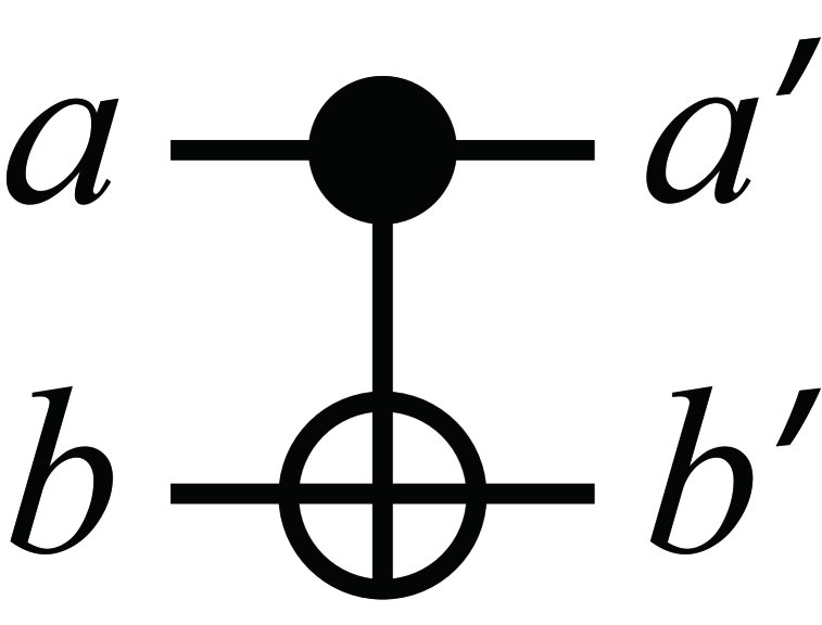
$abc$	$a^{\prime}b^{\prime}c^{\prime}$
000	000
001	001
010	010
011	011
100	100
101	101
110	111
111	110

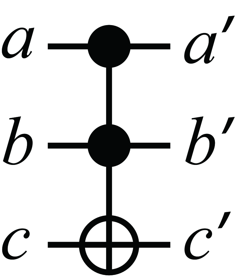
Figure 1: Truth tables and circuit symbols for CNOT (left) and Toffoli (right) gates.

Naturally, CNOT can be generalized to take $m+1$ input bits with $m$ controls and one target. It is sometimes called an MCT gate [24]. Let $C^{m}\!X$ denote such gates where $m$ is a non-negative integer. Since NCT gates are already included in MCT library (as with $m=0,1,2$), MCT library is also a universal set.

A $C^{m}\!X$ gate with $m>2$ can be decomposed into a few NCT gates with various tradeoffs. One may think of it as a conversion formula from an MCT gate to NCT gates. For example, $C^{m}\!X$ can be constructed by using $2m-3$ Toffoli gates with $m-2$ zeroed work bits, or by using $8m-24$ Toffoli gates with one arbitrary work bit [3]. Fig. 2 illustrates the former formula.

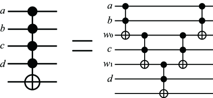
Figure 2: Decomposition of $C^{4}\!X$ into five ($=2\cdot 4-3$) Toffoli gates. Here $a,b,c,d$ are input control bits and $w_{0},w_{1}$ are zeroed work bits.

The number of Toffoli gates presented in a circuit will be regarded as the quality of it. Note that the quality gets better as the number of Toffoli gates decreases. An algorithm we design primarily uses MCT library, but then to measure the number of Toffoli gates, we need a certain conversion formula for all $C^{m}\!X$ gates with $m>2$. For this purpose, we will use a simple formula described in Fig. 2.

2.2 Permutation Circuit Synthesis

Having an appropriate basis, an $n$-bit permutation written in one-line notation $(r_{0},r_{1},\ldots,r_{2^{n}-1})$ can be seen as a matrix in $\{0,1\}^{2^{n}\times 2^{n}}$. For example for $n=3$ with the standard basis ${\bm{b}}_{0}=(1\;0\;0\;0\;0\;0\;0\;0)^{\top}$, ${\bm{b}}_{1}=(0\;1\;0\;0\;0\;0\;0\;0)^{\top},\cdots$, a permutation $P_{3}=(7,2,0,1,5,3,6,4)$ can be written by a truth table and by a matrix

000111001010010000011001100101101011110110111100,P3=(0010000000010000010000000000010000000001000010000000001010000000),fragments 000111001010010000011001100101101011110110111100subscript𝑃30010000000010000010000000000010000000001000010000000001010000000\displaystyle\begin{tabular}[]{c|c}\text{in}&\text{out}\\ \hline\cr 000&111\\ 001&010\\ 010&000\\ 011&001\\ 100&101\\ 101&011\\ 110&110\\ 111&100\\ \end{tabular},\quad P_{3}=\left(\begin{array}[]{>{\centering}p{0.1mm} >{\centering}p{0.1mm} >{\centering}p{0.1mm} >{\centering}p{0.1mm} >{\centering}p{0.1mm} >{\centering}p{0.1mm} >{\centering}p{0.1mm} c}0\@add@centering&0\@add@centering&1\@add@centering&0\@add@centering&0\@add@centering&0\@add@centering&0\@add@centering&0\\ 0\@add@centering&0\@add@centering&0\@add@centering&1\@add@centering&0\@add@centering&0\@add@centering&0\@add@centering&0\\ 0\@add@centering&1\@add@centering&0\@add@centering&0\@add@centering&0\@add@centering&0\@add@centering&0\@add@centering&0\\ 0\@add@centering&0\@add@centering&0\@add@centering&0\@add@centering&0\@add@centering&1\@add@centering&0\@add@centering&0\\ 0\@add@centering&0\@add@centering&0\@add@centering&0\@add@centering&0\@add@centering&0\@add@centering&0\@add@centering&1\\ 0\@add@centering&0\@add@centering&0\@add@centering&0\@add@centering&1\@add@centering&0\@add@centering&0\@add@centering&0\\ 0\@add@centering&0\@add@centering&0\@add@centering&0\@add@centering&0\@add@centering&0\@add@centering&1\@add@centering&0\\ 1\@add@centering&0\@add@centering&0\@add@centering&0\@add@centering&0\@add@centering&0\@add@centering&0\@add@centering&0\end{array}\right),

inoutinout (2.18)

where we have used the same symbol $P_{n}$ interchangeably to denote the one-line notation of an $n$-bit permutation and the corresponding matrix. Having it in mind, we define permutation circuit synthesis as follows:

Definition 2.1

For an $n$-bit permutation $P_{n}$, a finite universal gate set $G$, and a cost metric on a set, permutation circuit synthesis is to find a finite ordered set $R=\{g_{i}\;|\;g_{i}\in G\}$ such that $P_{n}\cdot\left(g_{1}\cdot g_{2}\cdot\cdots\cdot g_{|R|}\right)=I_{2^{n}}$, minimizing the cost on $R$.

Let $X_{i}$ denote a NOT gate acting on $i$-th bit, $C\!X_{ij}$ denote a CNOT gate controlled by $i$-th bit acting on $j$-th, $C\!X_{ijk}$ denote a Toffoli gate controlled by $i$- and $j$-th bits acting on $k$-th bit. One can verify that $P_{3}\cdot C\!X_{13}\cdot C\!X_{312}\cdot X_{2}\cdot C\!X_{23}\cdot C\!X_{231}=I_{2^{3}}$ (see, Eq (3.2) for gate actions), and thus $C\!X_{231}\cdot C\!X_{23}\cdot X_{2}\cdot C\!X_{312}\cdot C\!X_{13}=P_{3}$ since NCT gates are involutory ($A=A^{-1},A\in\text{NCT}$). At this point, a circuit for $P_{3}$ is synthesized but it can be questioned if the circuit is optimal under a certain cost metric. In fact, the optimality of 3- and 4-bit permutations under certain cost metrics has been proved by using exhaustive search [16] or meet-in-the-middle technique [9], but for larger $n$ no known result has claimed it.

When a permutation is structured it is often possible to find an efficient circuit by exploiting its structure. Here by ‘structured’ we mean $r_{i}$ is efficiently computable such that $r_{i}=f(i)$ with some function $f$. If such function is known, one may design a circuit that computes $f$ reversibly. A good example would be an eight-bit S-box used in the symmetric block cipher AES algorithm that can be calculated by arithmetic operations [23, 10].

On the other hand, when a permutation shows no apparent structure there is no known efficient method to synthesize it. The remaining options are to apply heuristic algorithms [27] or reversible lookup table methods [30]. A reversible lookup table is to implement each $r_{i}$ for corresponding $i$ one-by-one, reversibly. Although straightforward and possibly not less efficient than heuristic algorithms asymptotically, the reversible lookup table method is not preferred over heuristic algorithms for the problems at hand to our consideration.

A large number of algorithms for reversible logic circuit synthesis have been proposed. A good review can be found in [27]. Due to the heuristic nature of the algorithms, benchmark pages have been established for performance comparisons [24, 17].

3 Basic Idea

The basic strategy this work has taken is to reduce the effective size of a matrix at each step by looking for a size reduction process, leaving one bit completely excluded from subsequent steps. The size reduction idea can then naturally be resulted in an algorithm for permutation circuit synthesis under a certain assumption. The assumption will be lifted in Section 4 leading to an algorithm that works for any permutation.

3.1 Matrix Size Reduction

Reversible gates acting on $n$ bits can be viewed as rank-$2n$ tensors [32]. Among them, there exist certain gates of which decomposition as a tensor product of smaller tensors can be found. For example, Walsh-Hadamard transformation acting on two bits can be represented as a $4\times 4$ matrix (or equivalently rank-$4$ tensor), which can also be decomposed into two $2\times 2$ matrices such as

$$H^{\otimes 2} =\frac{1}{2}\left(\begin{array}[]{cccc}1&1&1&1\\ 1&-1&1&-1\\ 1&1&-1&-1\\ 1&-1&-1&1\\ \end{array}\right)$$ (3.23)

$$=\frac{1}{\sqrt{2}}\left(\begin{array}[]{cc}1&1\\ 1&-1\\ \end{array}\right)\otimes\frac{1}{\sqrt{2}}\left(\begin{array}[]{cc}1&1\\ 1&-1\\ \end{array}\right)\enspace.$$ (3.28)

However, CNOT cannot be written in terms of a simple tensor product of two smaller tensors.

Now consider a permutation $P_{n}$ that can be written as $P_{n-1}\otimes I_{2}$. It means the gate $P_{n}$ acts nontrivially on $n-1$ bits only, effectively leaving one bit irrelevant from the operation. It is clear that if one is able to find a procedure for transforming an arbitrary rank-$2n$ tensor into one that can be decomposed into one rank-($2n-2$) tensor and one $2\times 2$ identity matrix, the circuit can be synthesized by iterating the procedure at most $n-1$ times.

Somewhat related notion has been examined in synthesizing unitary matrices [19, 26], but apart from the use of the notion block (see, Section 3.2), the design criteria are quite different. In a nutshell, their method is to divide a large circuit into several smaller circuits and each one is recursively divided into even smaller ones, involving gate operations to every bit all the way through to the end. On the contrary, each time the size of the permutation gets smaller in our method, one bit becomes completely irrelevant from the circuit.

3.2 Definitions and Conventions

In $n$-bit permutation circuit synthesis, a gate set we use consists of $C^{m}\!X$ gates, where the number of control bits ranges from 0 to $n-1$.

Dealing with a permutation is probably best comprehensible in matrix representation as in Eq. (2.18), with an obvious downside that it is inconvenient to write down. One-line notation is thus frequently adopted throughout the paper. For example, the action of $X_{1}$, $C\!X_{21}$, and $C\!X_{312}$ on $(7,2,0,1,5,3,6,4)$ reads

$$\overset{X_{1}}{~{}~{}\longmapsto~{}~{}}\left(\hbox{\pagecolor[rgb]{0.7,0.7,0.7}\makebox(30.0,6.0)[]{$5,3,6,4$}},\hbox{\pagecolor[rgb]{0.7,0.7,0.7}\makebox(30.0,6.0)[]{$7,2,0,1$}}\right),$$

$$(7,2,0,1,5,3,6,4) \overset{C\!X_{21}}{~{}~{}\longmapsto~{}~{}}\left(7,2,\hbox{\pagecolor[rgb]{0.7,0.7,0.7}\makebox(11.0,6.0)[]{$6,4$}},5,3,\hbox{\pagecolor[rgb]{0.7,0.7,0.7}\makebox(11.0,6.0)[]{$0,1$}}\right),$$ (3.29)

$$\overset{C\!X_{312}}{~{}~{}\longmapsto~{}~{}}\left(7,2,0,1,5,\hbox{\pagecolor[rgb]{0.7,0.7,0.7}\makebox(1.5,6.0)[]{$4$}},6,\hbox{\pagecolor[rgb]{0.7,0.7,0.7}\makebox(1.5,6.0)[]{$3$}}\right).$$

When a permutation is written by $P_{n}=(r_{0},r_{1},...,r_{2^{n}-1})$, the subscripts $i$ and integers $r_{i}$ are understood as column numbers and row numbers, respectively, in which nonzero values reside in the matrix representation. For example, $r_{0}=7$ means 1 is located at the 0th column and the 7th row in the matrix as in Eq. (2.18). Using these notions, a permutation $P_{n}$ can be viewed as a function of a column number,

$$P_{n}:\{0,1,\cdots,2^{n}-1\}\rightarrow \,\{0,1,\cdots,2^{n}-1\},$$

$$i~{}~{}~{}~{}~{}\mapsto ~{}~{}~{}~{}~{}r_{i}.$$

Column numbers will frequently be read as $n$-bit binary strings. Binary strings will be denoted by vector notation when necessary. In writing an integer $x$ as an $n$-bit binary string ${\bm{x}}\in\{0,1\}^{n}$, we let $x_{i}\in\{0,1\}$ denote the $i$-th bit of ${\bm{x}}$ for $1\leq i\leq n$.

One way to understand the action of a logic gate is to think of it as an operator that exchanges column numbers. When a gate is applied, it first reads column numbers as $n$-bit binary strings. Among the strings (columns), some must meet the condition for the activation of the gate. The row numbers reside in these columns are swapped appropriately. For example in Eq. (3.2), each column number is read as $000,001,\cdots,111$ which are occupied by row numbers $7,2,\cdots,4$, respectively. The gate $C\!X_{132}$ is activated when the value of the first and the third bits are both 1, which correspond to the 5th (101) and the 7th (111) columns. The row numbers 3 and 4 which preoccupied these positions are then swapped by the gate.

In addition to $X_{i}$, $C\!X_{ij}$, and $C\!X_{ijk}$ gates defined in Section 2.2, we introduce a way to specify control and target bits of general $C^{m}\!X$ gates with nonnegative integer $m$. Let $\mathcal{I}$ be a subset of $\{1,\cdots,n\}$. In denoting a controlled gate with an arbitrary number of control bits, an index set $\mathcal{I}$ will be used such that $C\!X_{\mathcal{I}:k}$ has $|\mathcal{I}|$ control bits specified by elements in $\mathcal{I}$ and targets $k$-th bit.

The following definition for block is the central notion in this work, and it is recommended to refer to the example in Eq. (3.46) before comprehending the formal definition.

Definition 3.1

For an $n$-bit permutation $\left(r_{0},\ldots,r_{2^{n}-1}\right)$, a pair of numbers $r_{2i}$ and $r_{2i+1}$ is defined as an even (odd) block if $r_{2i+1}-r_{2i}=1\;(-1)$, where $i\in\{0,1,...,2^{n-1}-1\}$ is called a block-wise position.

It is unlikely that the number of blocks found in an unstructured permutation is large. It is then our task to find a transformation to maximize the number. For example, assume there is a map applied to a permutation matrix in Eq. (2.18) as follows:

$$\left({\begin{array}[]{cccccccc}0&0&1&0&0&0&0&0\\ 0&0&0&1&0&0&0&0\\ 0&1&0&0&0&0&0&0\\ 0&0&0&0&0&1&0&0\\ 0&0&0&0&0&0&0&1\\ 0&0&0&0&1&0&0&0\\ 0&0&0&0&0&0&1&0\\ 1&0&0&0&0&0&0&0\end{array}}\right)\mapsto\left({\begin{array}[]{cc:cc:cc:cc}0&0&0&0&0&0&\pagecolor[rgb]{0.7,0.7,0.7}0&\pagecolor[rgb]{0.7,0.7,0.7}1\\ 0&0&0&0&0&0&\pagecolor[rgb]{0.7,0.7,0.7}1&\pagecolor[rgb]{0.7,0.7,0.7}0\\ \hdashline\pagecolor[rgb]{0.7,0.7,0.7}1&\pagecolor[rgb]{0.7,0.7,0.7}0&0&0&0&0&0&0\\ \pagecolor[rgb]{0.7,0.7,0.7}0&\pagecolor[rgb]{0.7,0.7,0.7}1&0&0&0&0&0&0\\ \hdashline 0&0&0&0&\pagecolor[rgb]{0.7,0.7,0.7}1&\pagecolor[rgb]{0.7,0.7,0.7}0&0&0\\ 0&0&0&0&\pagecolor[rgb]{0.7,0.7,0.7}0&\pagecolor[rgb]{0.7,0.7,0.7}1&0&0\\ \hdashline 0&0&\pagecolor[rgb]{0.7,0.7,0.7}0&\pagecolor[rgb]{0.7,0.7,0.7}1&0&0&0&0\\ 0&0&\pagecolor[rgb]{0.7,0.7,0.7}1&\pagecolor[rgb]{0.7,0.7,0.7}0&0&0&0&0\end{array}}\right).$$ (3.46)

The $2\times 2$ substructures in gray color are called blocks. Even (odd) blocks are $2\times 2$ identity (off-diagonal) structures. In one-line notation of the resulting matrix $(2,3,7,6,4,5,1,0)$, pairwise row numbers 2, 3 and 4, 5 are even blocks and 7, 6 and 1, 0 are odd blocks.

These pairs of row numbers play an important role hereafter, but there is a chance the notions confuse readers. To avoid confusion, let us describe a way to construct an even block ‘$2,3$’ beginning from $(7,2,0,1,5,3,6,4)$. Using the $r_{i}$ notation, initially we have the pair $r_{1}=2$ and $r_{5}=3$. First, we want to put 2 in the 0th column. Applying $X_{1}C\!X_{13}X_{1}$ leads to $(2,7,1,0,5,3,6,4)$. This procedure can be interpreted as moving row number 2 from column position 1 to 0; $r_{1}\mapsto r_{0}$. Similarly, applying $C\!X_{31}$ then results in $(2,3,1,4,5,7,6,0)$; $r_{5}\mapsto r_{1}$. As already explained, applying gates can be interpreted as exchanging column numbers for fixed row numbers. All the algorithms and subroutines introduced below have similar descriptions that, first targeting a certain pair of row numbers, and then changing their column positions. At this point, let us formally define such pairs.

Definition 3.2

A pair of row numbers $2j,2j+1$ for $0\leq j\leq 2^{n-1}-1$ is called a relevant row pair, denoted by $\langle 2j,2j+1\rangle$.

Row numbers comprising a relevant row pair are called relevant row numbers. Constructing a block is thus putting relevant row numbers appropriately side-by-side that are originally located apart.

In addition, we further define the following:

Definition 3.3

For a relevant row pair $\langle r_{i},r_{j}\rangle$, the row numbers $r_{i}$ and $r_{j}$ are said to be occupied at

• normal positions if $r_{i}\equiv i$ and $r_{j}\equiv j\mod 2$.

• inverted positions if $r_{i}\not\equiv i$ and $r_{j}\not\equiv j\mod 2$.

• interrupting positions otherwise.

To better understand the definitions, consider a permutation $(\hbox{\pagecolor[rgb]{0.7,0.7,0.7}\makebox(5.0,6.0)[]{$7$}},\framebox{$2$},\hbox{\pagecolor[rgb]{0.7,0.7,0.7}\makebox(5.0,6.0)[]{$0$}},\framebox{$1$},\hbox{\pagecolor[rgb]{0.7,0.7,0.7}\makebox(5.0,6.0)[]{$5$}},\framebox{$3$},\hbox{\pagecolor[rgb]{0.7,0.7,0.7}\makebox(5.0,6.0)[]{$6$}},\framebox{$4$})$ and examine the relevant row pairs. Relevant row numbers $r_{2}=0$ and $r_{3}=1$ are at normal positions as $2\equiv_{2}0$ and $3\equiv_{2}1$. Another relevant numbers $r_{7}=4$ and $r_{4}=5$ are at inverted positions as $7\not\equiv_{2}4$ and $4\not\equiv_{2}5$. Other numbers are at interrupting positions. In simple terms, 0 and 1 are at normal positions as the small one is in the gray box, 4 and 5 are at inverted positions as the small one is in the white box, and other numbers are at interrupting positions as the numbers are in the same colored boxes.

It may seem plausible that the relevant numbers in normal (inverted) positions in the beginning likely end up in even (odd) blocks in the series of transformations for maximizing the number of blocks. Indeed if we are careful enough, all the row numbers in the normal (inverted) positions in the beginning form even (odd) blocks at the end. A formal description for the observation is as follows:

Remark 3.1

When $C^{m}\!X$ gate is applied, the number of normal, inverted, and interrupting positions is conserved unless the gate is targeting the $n$-th bit.

For example, a permutation $(7,2,0,1,5,3,6,4)$ has four row numbers at interrupting positions; 2, 3 and 7, 6. The action of $C\!X_{32}$ that does not target the 3rd bit leads to the permutation $(7,1,0,2,5,4,6,3)$, which still has four interrupting positions. On the other hand, if $C\!X_{13}$ is applied, the resulting permutation $(7,2,0,1,3,5,4,6)$ will no longer involve any interrupting position, but instead, the number of normal and inverted positions will be increased by two each. Details will not be covered, but we would point out that handling the interrupting positions is typically more expensive than dealing with normal or inverted positions. Therefore in the next section, a preprocess that removes interrupting positions before getting into the main process will be introduced. A way to deal with the inverted positions will also be introduced in the next section. For now, let us restrict our attention to permutations that only have normal positions. It will soon turn out that reversible gates targeting the last bit are not required at all in this section.

A natural way to design an algorithm for the size reduction could be to build blocks one-by-one, without losing already built ones. Remind that in one-line notation for a given permutation $(\framebox{$r_{0},r_{1}$},\framebox{$r_{2},r_{3}$},\framebox{$r_{4},r_{5}$},\framebox{$r_{6},r_{7}$},\cdots)$, a block is a pair of row numbers $r_{i}$ that differ by 1 (with the odd one being larger) and both reside in one of the designated column positions (boxes). Applying reversible gate swaps positions of at least two row numbers as in Eq. (3.2). What we want to do is to construct a new block while maintaining already constructed ones, which very much resembles solving Rubik’s Cube. Each rotation in Rubik’s Cube corresponds to the application of a logic gate. The difference is that while the number of rotations is to be minimized typically in Rubik’s Cube, we try to minimize the number of Toffoli gates.

3.3 Glossary

All necessary definitions and notations have been introduced, which we summarize below.

$X_{i}$, $C\!X_{ij}$, $C\!X_{ijk}$	NCT gates (Section 2.2)
$C\!X_{\mathcal{I}:k}$	MCT gates (Section 2.1)
$R$	An ordered set of gates
$P_{n}$	An $n$-bit substitution map
$(r_{0},r_{1},\ldots,r_{2^{n}-1})$	One-line notation of $P_{n}$
Row number $r_{i}$	Below Eq. (3.2)
Column number $i$ (of $r_{i}$)	Below Eq. (3.2)
Block	Definition 3.1
Block-wise position	Definition 3.1
Relevant row pair	Definition 3.2
Relevant row numbers	Below Definition 3.2
Normal position	Definition 3.3
Inverted position	Definition 3.3
Interrupting position	Definition 3.3
${\bm{x}}$	Binary string of an integer $x$
$x_{i}$	The $i$-th bit of ${\bm{x}}$ for $1\leq i\leq n$
Quality	In Section 2.1

3.4 Size Reduction Algorithm

In this section we restrict our attention to a procedure $\mathcal{A}^{\prime}_{\rm red}:\mathcal{P}^{\prime}_{n}\rightarrow\{P_{n}:P_{n}=P_{n-1}\otimes I_{2}\}\times\mathcal{R}$, where $\mathcal{P}^{\prime}_{n}$ is a set of all $n$-bit permutations of which row numbers are only in normal positions and $\mathcal{R}$ is a set of all ordered set of MCT gates. The algorithm $\mathcal{A}_{\rm red}^{\prime}$ is designed obeying three rules.

• A block is constructed one-by-one.

• The constructed block is allocated to the left in one-line notation.

• The number of left-allocated blocks should not decrease upon the action of any gate.

The meaning of the construction and the allocation is given in an example. Assume a three-bit permutation $P_{3}=(0,1,6,3,2,5,4,7)$ is at hand. The first block is already there, and we target the next block $(4,5)$. Applying $C\!X_{312}$ results in $P_{3}\cdot C\!X_{312}=(0,1,6,3,2,7,\hbox{\pagecolor[rgb]{0.7,0.7,0.7}\makebox(11.0,6.0)[]{$4,5$}})$. One can see that a new block is constructed in the 6th and the 7th columns at the cost of one Toffoli gate. The constructed block is then allocated in the 2nd and the 3rd columns by applying $C\!X_{21}$, i.e., $P_{3}\cdot C\!X_{312}\cdot C\!X_{21}=(0,1,\hbox{\pagecolor[rgb]{0.7,0.7,0.7}\makebox(11.0,6.0)[]{$4,5$}},2,7,6,3)$. In this example, only the construction costs a Toffoli gate whereas the allocation does not, but in general allocation also costs Toffoli gates. In spite of seemingly unnecessary cost for the allocation, we conclude that the left-allocation is more beneficial than leaving a block where it is constructed. Detailed reasonings for the left-allocation will not be covered .

In describing algorithms and subroutines, operations that update the permutation or the gate sequence will be frequently involved. For a permutation $P_{n}$, an ordered set of gates $R=(a_{1},\ldots,a_{|R|})$, and an another ordered set of gates $S=(b_{1},\ldots,b_{|S|})$, define a symbol $\cdot$ such that

$$(P_{n},R)\cdot S =\left(P_{n}\cdot b_{1}\cdot b_{2}\cdot\ldots\cdot b_{|S|},(R;S)\right),$$

$$(R;S) =(a_{1},\ldots,a_{|R|},b_{1},\ldots,b_{|S|}).$$

High-level description of the size reduction algorithm is as follows:

Algorithm 1 $\mathcal{A}_{\rm red}^{\prime}$

Input $P_{n}$ $\triangleright$ $P_{n}\in\mathcal{P}^{\prime}_{n}$
      Output $(P,R)$ $\triangleright$ $P=P_{n-1}\otimes I_{2}$
      Procedure

1:$R\leftarrow\left(~{}\right)$ $\triangleright$ An empty ordered set

2:$P\leftarrow P_{n}$

3:for $i$ from $0$ to $2^{n-1}-1$ do

4:     $\langle a,b\rangle\leftarrow$ PICK$(P,i)$ $\triangleright$ Pick a relevant row pair

5:     $\textit{S}_{C}\leftarrow$ CONS($P$, $i$, $\langle a,b\rangle$)

6:     $(P,R)\leftarrow(P,R)\cdot S_{C}$

7:     $\textit{S}_{A}\leftarrow$ ALLOC($P$, $i$, $a$)

8:     $(P,R)\leftarrow(P,R)\cdot S_{A}$

9:return $(P,R)$

It will be helpful to have some intuition behind the details before describing the subroutines PICK, CONS, and ALLOC. Define $m$ as the smallest positive integer satisfying

$$2l\leq\sum_{j=1}^{m-1}2^{n-j},$$ (3.47)

where $l$ is the number of left-allocated blocks and we define $m=1$ for $l=0$. A pattern how $m$ is determined depending on $l$ is illustrated in Fig. 3. Now notice that a group of left-allocated blocks distinguished by dashed lines in the figure shares the same bit values in their column numbers as $n$-bit binary strings. For example, from $i=0$ to $2^{n-2}-1$ in the figure, the first bit of the column numbers is zero. From $i=2^{n-2}$ to $2^{n-2}+2^{n-3}-1$, the first bit is one and the second bit is zero. The point is, in constructing a new block, the (already) left-allocated blocks have some common properties. The properties can be exploited to build a block without too much cost being paid, which we shall prove in Section 3.5 to be upper bounded by one $C^{m}\!X$ and a few $C\!X$ and $X$ gates.

In constructing a new block in the $i$-th iteration where $i$ is the iterator in Algorithm 1, not all remaining relevant row pairs can be constructed as a block meeting the bound. However, it can be shown that at least one pair that meets the bound always exists for all $i$. Subroutine PICK takes care of passing an appropriate pair to CONS and ALLOC such that the quality bound can be met.

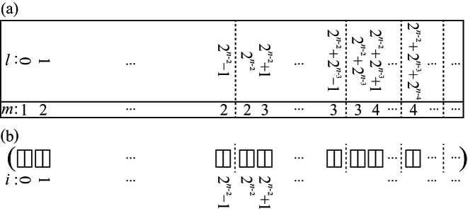
Figure 3: (a) Relation between $m$ and $l$. (b) Column positions (rectangle) and block-wise positions (two conjoined rectangles) in a permutation. Constructed blocks are to be allocated to the left, occupying block-wise positions denoted by $i$. When one tries to construct and allocate a new block at $i$-th position, $l$ equals $i$ and thus $m$ is determined as specified. Dashed vertical lines divide the number of column positions to be as ratios 1:1, 3:1, 7:1, and so on.

Allocation is similar to construction. Let $\oplus$ denote the bit-wise XOR of binary strings. Suppose we are to construct a block by conjoining two relevant row numbers of which column numbers are $\alpha$ and $\beta$, respectively, where ${\bm{\alpha}}\oplus{\bm{\beta}}\in\{0,1\}^{n}$. Construction can be understood as a process of changing $\alpha$ and $\beta$ so that ${\bm{\alpha}}\oplus{\bm{\beta}}=00\cdots 01$, without breaking left-allocated blocks. By breaking, we mean some of the previously left-allocated blocks are no longer left-allocated, or the number of left-allocated blocks decreases. Now, suppose we successfully constructed a block with the aforementioned relevant row pair, and we want to allocate it to the $i$-th block-wise position. Let $c_{i}$ denote one of the column numbers at $i$-th block-wise position (regular squares in Fig. 3). Allocation is a process of changing $\alpha$ so that ${\bm{c}}_{i}\oplus{\bm{\alpha}}=00\cdots 0\!*~{}(*\in\{0,1\})$, without breaking left-allocated blocks and with preserving ${\bm{\alpha}}\oplus{\bm{\beta}}=00\cdots 01$. Therefore ALLOC is more or less the same as CONS, and it will be shown in detail that in allocating a constructed block to $i$-th block-wise position, the cost is upper bounded by $C^{s(i)}\!X$ and a few $C\!X$ and $X$ gates, where $s(i)$ is a function such that $s(i)\leq HW({\bm{i}})$, where $HW({\bm{i}})$ is the hamming weight of ${\bm{i}}$.

We first describe PICK.

Subroutine 1 PICK

Input $P_{n}$, $i$
      Output $\langle a,b\rangle$
      Procedure

1:$m\leftarrow$ FINDM($i$)

2:$k\leftarrow 2^{n}-2^{n-m+1}$

3:for $j$ from $k$ to $2^{n}-2$ do

4:     $a\leftarrow r_{j}$

5:     $b\leftarrow{\bm{a}}\oplus{\bm{1}}$ $\triangleright$ ${\bm{1}}=00\ldots 01$

6:     for $t$ from $j+1$ to $2^{n}-1$ do

7:         $c\leftarrow r_{t}$

8:         if $b=c$ then

9:              return $\langle a,b\rangle$               

Termination of the subroutine will be shown to be guaranteed in the next subsection. In line 1, FINDM computes $m$ from $i$ by letting $l=i$ in Eq. (3.47).

Now we describe CONS.

Subroutine 2 CONS

Input $P_{n},i,\langle a,b\rangle$
      Output $S_{C}$
      Procedure

1:$S_{C}\leftarrow(~{})$ $\triangleright$ An empty ordered set

2:$m\leftarrow$ FINDM($i$)

3:$(\alpha,\beta)\leftarrow$ COL($P_{n},a,b$) $\triangleright$ Find​ column​ numbers

4:${\bm{\gamma}}\leftarrow{\bm{\alpha}}\oplus{\bm{\beta}}$

5:$\delta\leftarrow 0$

6:for $j$ from $1$ to $n$ do

7:     if $\gamma_{j}=1$ then

8:         $\delta\leftarrow j$

9:         break      

10:if $\delta=n$ then

11:     return $S_{C}$ $\triangleright$ Already a block

12:if $i_{\delta}=1$ then

13:     $S_{C}\leftarrow S_{C};X_{\delta}$ $\triangleright$ Append $X_{\delta}$ to $S_{C}$

14:for $j$ from $\delta+1$ to $n-1$ do

15:     if $\gamma_{j}=1$ then

16:         $S_{C}\leftarrow S_{C};C\!X_{\delta j}$      

17:if $i_{\delta}=1$ then

18:     $S_{C}\leftarrow S_{C};X_{\delta}$

19:$\mathcal{I}\leftarrow\{n\}$

20:for $j$ from 1 to $m-1$ do

21:     $\mathcal{I}\leftarrow\mathcal{I}\cup\{j\}$

22:$S_{C}\leftarrow S_{C};C\!X_{\mathcal{I}:\delta}$

23:return $S_{C}$

In line 3, COL outputs column numbers $\alpha,\beta$ corresponding to the relevant row numbers $a,b$. This procedure is necessary since what CONS essentially does is to swap columns as mentioned earlier.

ALLOC is similarly described.

Subroutine 3 ALLOC

Input $P_{n},i,a$
      Output $S_{A}$
      Procedure

1:$S_{A}\leftarrow(~{})$

2:$m\leftarrow$ FINDM($i$)

3:$\alpha\leftarrow$ COL($P_{n},a$)

4:${\bm{\gamma}}\leftarrow{\bm{\alpha}}\oplus{\bm{i}}$

5:$\delta\leftarrow 0$

6:for $j$ from $1$ to $n$ do

7:     if $\gamma_{j}=1$ then

8:         $\delta\leftarrow j$

9:         break      

10:if $\delta=0$ then

11:     return $S_{A}$ $\triangleright$ Already allocated

12:$\mathcal{I}\leftarrow\{~{}\}$

13:for $j$ from $\delta+1$ to $n-1$ do

14:     if $\gamma_{j}=1$ then

15:         $S_{A}\leftarrow S_{A};C\!X_{\delta j}$      

16:     if $i_{j}=1$ then

17:         $\mathcal{I}\leftarrow\mathcal{I}\cup\{j\}$      

18:$S_{A}\leftarrow S_{A};C\!X_{\mathcal{I}:\delta}$

19:return $S_{A}$

3.5 Quality and Complexity

It has been sketched in Section 3.4 how the size reduction algorithm works. Here we evaluate the time complexity and the quality of the output by introducing two lemmas, one for the construction and the other for the allocation.

Proposition 3.1

Let $l$ be the number of left-allocated blocks, and $m$ be the smallest positive integer satisfying Eq. (3.47). Define a function $h_{n}:\mathbb{N}\rightarrow\mathbb{Z}$, $h_{n}(x)=2^{n}-2^{n-(x-1)}$. There exists at least one relevant row pair $r_{\alpha},r_{\beta}$ such that

$$h_{n}(m)<\min(\alpha,\beta),$$ (3.48)

where $\alpha,\beta$ are column numbers of $r_{\alpha},r_{\beta}$, respectively.

• It is nothing more than Pigeonhole principle. It is trivial for $m=1$. For $m>1$, there exist $2^{n}-2l$ row numbers that do not form left-allocated blocks, yet. Let us call them the remaining row numbers (row pairs). Assume there is no remaining row pair satisfying Eq. (3.48). Then at least one relevant row number in every remaining pair has to sit in column numbers no greater than $h_{n}(m)$. However, since $2l$ column numbers are already occupied by left-allocated blocks, there only exist $h_{n}(m)-2l$ columns available for the row numbers to sit in. If we subtract $h_{n}(m)-2l$ from half the number of remaining row numbers $(2^{n}-2l)/2$,

  $$\frac{(2^{n}-2l)}{2}-\left(h_{n}(m)-2l\right) =l-\frac{h_{n}(m-1)}{2}$$

  $$>0,$$

  where the inequality follows from the fact that $h_{n}(m-1)<2l\leq h_{n}(m)$ by the definition of $m$. Therefore the assumption cannot be true and there must exist at least one pair that satisfies Eq. (3.48).

Lemma 3.1

Let $i$ be an iterator used in Algorithm 1, $l$ be the number of left-allocated blocks, and $m$ be the smallest positive integer satisfying Eq. (3.47). For given permutation, a new block can be constructed by using at most $n-m-1$ $C\!X$, two $X$, and one $C^{m}\!X$ gates, without breaking left-allocated blocks.

• Let $\mathcal{C}=\{0,1,\cdots,2^{n-1}-1\}$ be a set of block-wise positions of an $n$-bit permutation, ${\bm{i}}$ be the binary string of $i\in\mathcal{C}$, and $r_{\alpha},r_{\beta}$ be relevant row numbers satisfying Eq. (3.48). Viewing their column numbers as binary strings ${\bm{\alpha}}$ and ${\bm{\beta}}$, the first $m-1$ bits of them are 1 (none if $m=1$),

  $$\alpha_{1}=\beta_{1}=\alpha_{2}=\beta_{2}=\cdots=\alpha_{m-1}=\beta_{m-1}=1.$$ (3.49)

  Let ${\bm{\gamma}}={\bm{\alpha}}\oplus{\bm{\beta}}$ and $\delta$ be the smallest integer such that $\gamma_{\delta}=1$. It can be seen that $\delta>m-1$. Assume $\delta\neq n$, otherwise, the pair is already a block. Let $L_{\delta}$, $R_{\delta}$ be disjoint subsets of $\mathcal{C}$ such that $\mathcal{C}=L_{\delta}\bigcup R_{\delta}$ and the blocks residing in $L_{\delta}$ and $R_{\delta}$ are preserved under the actions of $C\!X_{\delta x}$ and $X_{\delta}C\!X_{\delta x}X_{\delta}$ gates for $x\in\{1,\ldots,\delta-1,\delta+1,\ldots,n\}$, respectively. A few $L_{\delta}$ and $R_{\delta}$ are illustrated in Fig. 4.

  

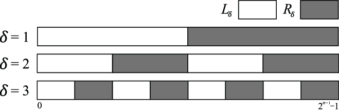
  Figure 4: $L_{\delta}$ and $R_{\delta}$ for $\delta=1,2,3$.

At $i$-th iteration, note that $i$ (as a block-wise number) is either included in $L_{\delta}$ or $R_{\delta}$. If $i\in L_{\delta}$, an action of $C\!X_{\delta x}$, $\delta<x<n$ gate does not break left-allocated blocks since the blocks in $L_{\delta}$ are not affected at all and the blocks in $R_{\delta}$ change their respective positions within $<i$. If on the other hand $i\in R_{\delta}$, similarly an action of $X_{\delta}C\!X_{\delta x}X_{\delta}$, $\delta<x<n$ gate does not break left-allocated blocks since the blocks in $R_{\delta}$ are conserved and the blocks in $L_{\delta}$ change their respective positions within $<i$. Because $i_{\delta}$ tells if it is included in $L_{\delta}$ or $R_{\delta}$, we are able to apply the aforementioned gates without breaking left-allocated blocks.

First $\delta-1$ bits of ${\bm{\gamma}}$ are zeros due to the definition of $\delta$. Since $C\!X_{\delta x}$ or $X_{\delta}C\!X_{\delta x}X_{\delta}$, $\delta<x<n$ gate can be applied without breaking the left-allocated blocks, it is always possible to achieve $\gamma_{\delta}=\gamma_{n}=1$ and $\gamma_{k}=0$ for all $k\not\in\{\delta,n\}$, without involving any Toffoli gate. Once it is achieved, by applying $C\!X_{\mathcal{I}:\delta}$, $\mathcal{I}=\{1,2,\cdots,m-1,n\}$, we have ${\bm{\gamma}}=00\cdots 01$, which is by definition a block. Blocks located left to $i$ are unaffected by $C\!X_{\mathcal{I}:\delta}$ gate since the binary strings of their positions have at least one zero among the first $m-1$ bits.

Lemma 3.2

Let $i$ be an iterator used in Algorithm 1, $l$ be the number of left-allocated blocks, and $m$ be the smallest positive integer satisfying Eq. (3.47). For given permutation with a block constructed by CONS, the block can be allocated to the $i$-th block-wise position by using at most $(n-m)$ $C\!X$ and one $C^{HW({\bm{i}}^{\prime})}\!X$ gates, without breaking left-allocated blocks, where $i^{\prime}=i-h_{n}(m-1)/2$ for $m>1$ and $i^{\prime}=i$ otherwise.

• Let ${\bm{j}}$ be a binary string of the (block-wise) position $j$ of the block constructed by CONS. Assume $j\neq i$, otherwise, the block is already left-allocated. Let ${\bm{\gamma}}={\bm{i}}\oplus{\bm{j}}$ and $\delta$ be the smallest integer such that $\gamma_{\delta}=1$. Due to the property of the column numbers we begin with in CONS, i.e., Eq. (3.48), the first $m-2$ bits of ${\bm{i}}$ and ${\bm{j}}$ are 1 (none if $m\leq 2$),

  $$i_{1}=j_{1}=i_{2}=j_{2}=\cdots=i_{m-2}=j_{m-2}=1,$$ (3.50)

  and thus $\delta>m-2$. Since $i<j$ and $\gamma_{1}=\gamma_{2}=\cdots=\gamma_{\delta-1}=0$, it is guaranteed that $i_{\delta}=0$ and $j_{\delta}=1$. Similar to the technique used in Lemma 3.1, ${\bm{j}}$ can be transformed such that $\gamma_{\delta}=1$ and $\gamma_{k}=0$ for all $k\not\in\{\delta\}$ by using $C\!X_{\delta x}$ gates for $\delta<x<n$. Note that unlike in Lemma 3.1 where ${\bm{\alpha}}$ and ${\bm{\beta}}$ both can be transformed by gates, here only ${\bm{j}}$ is allowed to change. Once it is done, by applying $C\!X_{\mathcal{I}:\delta}$, $\mathcal{I}=\{x\,|\,x>\delta,\;i_{x}=1\}$, the left-allocation is completed. Note that blocks residing in $L_{\sigma}$, $\sigma\in\{x\,|\,x<\delta,\;i_{x}=1\}$ are conserved by an action of a gate whose target is $\delta$-th bit, up to changes of block-wise positions within. In addition, by the definition of $L_{\sigma}$, $i$ cannot be included in any of $L_{\sigma}$. Therefore, $C\!X_{\mathcal{I}:\delta}$ can be applied without breaking the left-allocated blocks.

Upper bounds on the number of Toffoli gates in the output circuit naturally follows from two lemmas. Be reminded that we have adopted the conversion formula $C^{m}\!X:C^{2}\!X=1:2m-3$. By counting the worst-case number of Toffoli gates in CONS and ALLOC for all iterations, it can be summarized as follows:

Theorem 3.1

The number of Toffoli gates in the output $R$ of Algorithm 1 is upper bounded by $\mathcal{N}_{c}(n)+\mathcal{N}_{a}(n)$ for $n\geq 3$, where

$$\mathcal{N}_{c}(n) =\sum_{i=2}^{n-1}\left(2i-3\right)\cdot 2^{n-i},$$

$$\mathcal{N}_{a}(n) =\sum_{j=2}^{n-2}{\sum_{i=2}^{n-j}\left(2i-3\right)\cdot{n-j\choose i}},$$ (3.51)

where $\mathcal{N}_{a}(3)=0$.

Time complexity of Algorithm 1 can also be estimated by the lemmas. Assuming all gates exchange $2^{n}$ column numbers (overestimation for $C^{m}\!X$ for $m>0$), the time complexity of the algorithm simply reads the total number of gates times $2^{n}$. The maximum number of gates applied in each CONS and ALLOC is $O(n)$, and the number of CONS and ALLOC called in Algorithm 1 is $2^{n-1}$ each, and thus the asymptotic time complexity reads $O(n2^{2n})$.

4 Algorithm

Key ideas have been introduced in Section 3. The only downside of Algorithm 1 is its inability to decompose arbitrary permutations. This section is therefore mostly devoted to lifting the assumption that an input permutation consists only of row numbers in normal positions. Lifting the assumption costs an extra number of Toffoli gates which is bounded by

$$5\cdot 2^{n-4}+2n-5+\sum_{i=2}^{n-3}\left(2i-3\right)\cdot{n-3\choose i}.$$ (4.52)

Lifting the assumption takes several independent steps, which we shall separately deal with in each subsection. Details on various formulas appearing in this section are more or less the same as in the previous section, and thus will mostly be dropped.

4.1 Heuristic Mixing

Throughout Section 4 we will frequently refer to the ratio of the number of normal, inverted, and interrupting positions as the ratio $x:y:z$ such that $x+y+z=1$. For example, all permutations handled in Section 3.4 have the ratio $1:0:0$.

The goal of the first step, Heuristic Mixing, is to transform an arbitrary permutation into one with the ratio $x:y:0.5$, where $x$ and $y$ are arbitrary. The method is to apply $C\!X$ gates a few times until the desired ratio is (nearly) achieved. The following assumption is based on an observation: unstructured or randomly chosen permutations have a ratio close to $x:y:0.5$.

Assumption 4.1

There exists a composite gate consisting of at most four $C\!X$ and one $C^{n-1}\!X$ gates that transforms a permutation such that the resulting permutation exhibits the ratio $x:y:0.5$.

Here we count $X_{i}C\!X_{ij}X_{i}$, $j\neq i$ (so called negative controlled gates) as $C\!X$ gate, too. Let us call a composite gate consisting of $t$ $C\!X$ gates a depth-$t$ composite. For example, counting the meaningful composites, there exist no depth-0 composites, $2n-2$ depth-$1$ composites, at most $(2n-2)\cdot 4{n\choose 2}$ depth-2 composites, and so on. As an algorithm, we may apply depth-$t$ composites one-by-one from $t=0$ to $t=4$ until the ratio hits $x:y:0.5$ exactly, or until all the composites are exhausted. When the latter happens, we choose a permutation among the tried ones that are closest to the desired ratio, and then apply one $C^{n-1}\!X$ gate to meet $x:y:0.5$.

We have carried out numerical tests on random samples for $t\in\{0,1,2,3\}$, plotting $\lambda-2^{n-1}$ (or $|\lambda-2^{n-1}|$), where $\lambda$ is the number of interrupting positions in a permutation we can get with depth-$t$ composites that is closest to the desired ratio. As the results in Fig. 5 show, applying a few $C\!X$ composites likely leads to the desired ratio.

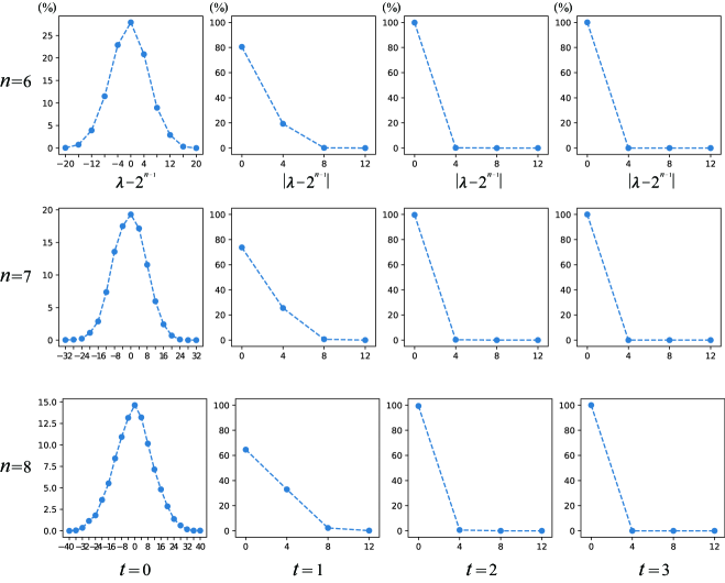
Figure 5: Sampling tests for $n\in\{6,7,8\}$ and $t\in\{0,1,2,3\}$. Each figure shows the percentage of samples as a function of $\lambda-2^{n-1}$ (or $|\lambda-2^{n-1}|$), where $\lambda$ is defined in the main text. In other words, figures show how far the permutations are from the ratio $x:y:0.5$ (and especially $\lambda-2^{n-1}=0$ means the ratio is exactly $x:y:0.5$). For $t=2$ where two CX gates have been applied, we were already able to find the desired permutations with high probability. The margin of error is $\pm 1.55$% at $95$% confidence level.

4.2 Preprocessing

The output of Heuristic Mixing is a permutation with the ratio $x:y:0.5$. It is then further processed by an algorithm $\mathcal{A}_{\rm pre}$ to be the ratio $0.5:0.5:0$.

The idea is simple and we give an example first. Consider the following $4$-bit permutation:

$$(3,\hbox{\pagecolor[rgb]{0.7,0.7,0.7}\makebox(5.0,6.0)[]{$10$}},14,6,\hbox{\pagecolor[rgb]{0.7,0.7,0.7}\makebox(5.0,6.0)[]{$12$}},2,\hbox{\pagecolor[rgb]{0.7,0.7,0.7}\makebox(2.0,6.0)[]{$0$}},15,5,\hbox{\pagecolor[rgb]{0.7,0.7,0.7}\makebox(2.0,6.0)[]{$8$}},\hbox{\pagecolor[rgb]{0.7,0.7,0.7}\makebox(5.0,6.0)[]{$13$}},\hbox{\pagecolor[rgb]{0.7,0.7,0.7}\makebox(2.0,6.0)[]{$9$}},\hbox{\pagecolor[rgb]{0.7,0.7,0.7}\makebox(2.0,6.0)[]{$1$}},4,7,\hbox{\pagecolor[rgb]{0.7,0.7,0.7}\makebox(5.0,6.0)[]{$11$}}),$$

where eight interrupting positions are highlighted. Move four of them to the left by a sequence of gates $C\!X_{13}$, $X_{1}$, $C\!X_{12}$, $C\!X_{13}$, $C\!X_{241}$, $C\!X_{32}$ in order, leading to

$$(\hbox{\pagecolor[rgb]{0.7,0.7,0.7}\makebox(5.0,6.0)[]{$13$}},\hbox{\pagecolor[rgb]{0.7,0.7,0.7}\makebox(2.0,6.0)[]{$9$}},\hbox{\pagecolor[rgb]{0.7,0.7,0.7}\makebox(2.0,6.0)[]{$1$}},\hbox{\pagecolor[rgb]{0.7,0.7,0.7}\makebox(5.0,6.0)[]{$10$}},7,6,5,\hbox{\pagecolor[rgb]{0.7,0.7,0.7}\makebox(2.0,6.0)[]{$8$}},\hbox{\pagecolor[rgb]{0.7,0.7,0.7}\makebox(2.0,6.0)[]{$0$}},15,3,4,14,\hbox{\pagecolor[rgb]{0.7,0.7,0.7}\makebox(5.0,6.0)[]{$11$}},\hbox{\pagecolor[rgb]{0.7,0.7,0.7}\makebox(5.0,6.0)[]{$12$}},2).$$

Applying another sequence $X_{1}$, $X_{2}$, $C\!X_{124}$, $X_{1}$, $X_{2}$ results in

$$(9,13,10,1,7,6,5,8,0,15,3,4,14,11,12,2).$$

Here we only sketch the mechanism, rather than elaborating on it. Due to the way the interrupting position is defined, it can only be an even number; (hypothetical) change of a ‘single’ row number leads to either $-2,+0$, or $+2$ change to the number of interrupting positions. Since at least two row numbers are exchanged by the logic gates, the number of interrupting positions can only vary by multiples of 4. Note that an action of $C^{n-1}\!X$ gate that swaps two row numbers can change the number of interrupting positions by at most 4. Considering along the line, an action of $C^{2}\!X$ gate that swaps $2^{n-2}$ row numbers can change the number by at most $2^{n-1}$. Since the number of interrupting positions of an input permutation is $2^{n-1}$, at best a single Toffoli can achieve the desired ratio. However, the best case hardly happens naturally, and we need to manipulate the input before applying the Toffoli gate. It is complicated to give details, but we claim that a procedure similar to repeating CONS and ALLOC one-quarter times of that of $\mathcal{A}^{\prime}_{\rm red}$ is enough. In addition to its ability to eliminate interrupting positions, the procedure can also fine-tune the number of normal and inverted positions. In fact, $\mathcal{A}_{\rm pre}$ can turn the ratio $x:y:0.5$ into $x\pm\Delta_{x}:y\pm\Delta_{y}:0$ where $0\leq\Delta_{x},\Delta_{y}\leq 0.5$. In the following algorithm $\mathcal{A}_{\rm pre}$, we may simply set the output ratio to be 0.5:0.5:0.

The procedure is described as follows:

Algorithm 2 $\mathcal{A}_{\rm pre}$

Input $P_{n}$ $\triangleright$ The ratio is $x:y:0.5$
      Output $(P,R)$
      Procedure

1:$R\leftarrow\left(~{}\right)$

2:$P\leftarrow P_{n}$

3:for $i$ from $0$ to $2^{n-3}-1$ do

4:     $\langle a,b\rangle\leftarrow$ PRE_PICK$(P,i)$

5:     $\textit{S}_{C}\leftarrow$ CONS($P$, $i$, $\langle a,b\rangle$)

6:     $(P,R)\leftarrow(P,R)\cdot S_{C}$

7:     $\textit{S}_{A}\leftarrow$ ALLOC($P$, $i$, $a$)

8:     $(P,R)\leftarrow(P,R)\cdot S_{A}$

9:$(P,R)\leftarrow(P,R)\cdot(X_{1},X_{2},C\!X_{12n},X_{2},X_{1})$

10:return $(P,R)$

PRE_PICK works in a similar way to PICK, but the output is not a relevant row pair but a certain pair of row numbers at interrupting positions. We will not cover the details on the pair, but with abuse of notation we let $\langle\cdot,\cdot\rangle$ denotes the pair, too. Interested readers may refer to the implemented code [1]. CONS and ALLOC work exactly the same way as in Section 3.4. The number of Toffoli gates involved in Algorithm 2 is bounded by $3\cdot 2^{n-4}-1+\sum_{i=2}^{n-3}\left(2i-3\right)\cdot{n-3\choose i}$.

4.3 Generalized Size Reduction Algorithm

After the mixing and the preprocessing, the permutation has the ratio $0.5:0.5:0$. Now the problem can be thought of as two subproblems. We will first construct and allocate only even blocks out of row numbers that are in normal positions. Since CONS and ALLOC do not require any controlled gate targeting the $n$-th bit, the number of normal or inverted positions is conserved by Remark 3.1. Once $2^{n-2}$ even blocks are left-allocated, the remaining row numbers that are only in inverted positions are constructed and allocated to be odd blocks. In the end, we would have $2^{n-2}$ even blocks on the left half and $2^{n-2}$ odd blocks on the right half. Applying one $C\!X_{1n}$ gate completes the size reduction.

The size reduction algorithm is described as follows:

Algorithm 3 $\mathcal{A}_{\rm red}$

Input $P_{n}$ $\triangleright$ The ratio is $0.5:0.5:0$
      Output $(P,R)$ $\triangleright$ $P=P_{n-1}\otimes I_{2}$
      Procedure

1:$R\leftarrow\left(~{}\right)$

2:$P\leftarrow P_{n}$

3:for $i$ from $0$ to $2^{n-2}-1$ do $\triangleright$ First Part

4:     $\langle a,b\rangle\leftarrow$ N_PICK$(P,i)$ $\triangleright$ Pick a normal pair

5:     $\textit{S}_{C}\leftarrow$ CONS($P$, $i$, $\langle a,b\rangle$)

6:     $(P,R)\leftarrow(P,R)\cdot S_{C}$

7:     $\textit{S}_{A}\leftarrow$ ALLOC($P$, $i$, $a$)

8:     $(P,R)\leftarrow(P,R)\cdot S_{A}$

9:for $i$ from $2^{n-2}$ to $2^{n-1}-1$ do $\triangleright$ Second Part

10:     $\langle a,b\rangle\leftarrow$ PICK$(P,i)$

11:     $\textit{S}_{C}\leftarrow$ CONS($P$, $i$, $\langle a,b\rangle$)

12:     $(P,R)\leftarrow(P,R)\cdot S_{C}$

13:     $\textit{S}_{A}\leftarrow$ ALLOC($P$, $i$, $a$)

14:     $(P,R)\leftarrow(P,R)\cdot S_{A}$

15:$(P,R)\leftarrow(P,R)\cdot(C\!X_{1n})$

16:return $(P,R)$

The first part deals with row numbers in normal positions to construct and allocate even blocks only. Therefore, N_PICK has to output a relevant row pair in normal positions. Accordingly, the working mechanism of N_PICK is a bit different from that of PICK [1]. Quality bounds given by Proposition 3.1, Lemma 3.1, and Lemma 3.2 are no longer valid in the first part, but overall it only adds $2^{n-3}$ to the quality bound of $\mathcal{A}^{\prime}_{\rm red}$. Details on N_PICK and related quality bound are not discussed here. The second part works exactly the same as Algorithm 1 except now the row numbers are only in inverted positions instead of normal positions.

The additional quality factor, $2^{n-3}$, can hardly be met in average instances, and in practice the quality difference between outputs of $\mathcal{A}^{\prime}_{\rm red}$ and $\mathcal{A}_{\rm red}$ is negligible.

Note that the point of mixing and preprocessing is to transform an arbitrary permutation so that the result has an appropriate form for the decomposition. If a given permutation is already well-suited for $\mathcal{A}^{\prime}_{\rm red}$, or $\mathcal{A}_{\rm red}$, or something similar, mixing and preprocessing can be skipped.

4.4 Algorithm for Synthesis

Combining Heuristic Mixing, Preprocessing, and $\mathcal{A}_{\rm red}$, one can easily come up with an algorithm for reversible logic circuit synthesis as follows:

Algorithm 4 $\mathcal{A}_{\rm syn}$

Input $P_{n}$
      Output $R$
      Procedure

1:$R\leftarrow\left(~{}\right)$

2:for $i$ from $n$ to 3 do

3:     $(P_{i},R_{\rm mix})\leftarrow\mathcal{A}_{\rm mix}(P_{i})$$\triangleright$ Heuristic Mixing

4:     $(P_{i},R_{\rm pre})\leftarrow\mathcal{A}_{\rm pre}(P_{i})$

5:     $(P_{i},R_{\rm red})\leftarrow\mathcal{A}_{\rm red}(P_{i})$

6:     $P_{i-1}\leftarrow$ REDUCE$(P_{i})$ $\triangleright$ $P_{i}=P_{i-1}\otimes I_{2}$

7:     $R\leftarrow R$;$R_{\rm mix}$;$R_{\rm pre}$;$R_{\rm red}$ $\triangleright$ Append all

8:$R\leftarrow R$;SEARCH$(P_{2})$ $\triangleright$ Exhaustive search for $P_{2}$

9:return $R$

Let the quality bound given by Theorem 3.1 be $A(n)$ and the cost Eq. (4.52) be $B(n)$ for an $n$-bit permutation. The number of Toffoli gates required for the size reduction $P_{n}\mapsto P_{n-1}$ is upper bounded by

$$A(n)+B(n).$$ (4.53)

Therefore the quality bound on the output $R$ of Algorithm 4 is given by $\sum_{x=n}^{3}\left(A(x)+B(x)\right)$.

Time complexity of $\mathcal{A}_{\rm mix}$ can be estimated by counting the number of composites times $2^{n}$, which reads $O(n^{7}2^{n})$. Preprocessing roughly does one-quarter of what the size reduction performs, thus the time complexity is $O(n2^{2n-2})$. Time complexities of $\mathcal{A}^{\prime}_{\rm red}$ and $\mathcal{A}_{\rm red}$ are the same. In $\mathcal{A}_{\rm syn}$, the first size reduction step dominates the overall running time because each time the effective size gets smaller, time to transform the permutation becomes exponentially faster. The time complexity of size reduction steps in $\mathcal{A}_{\rm syn}$ is dominated by $\mathcal{A}_{\rm red}$ with $O(n2^{2n})$, thus the time complexity of $\mathcal{A}_{\rm syn}$ is $O(n2^{2n})$.

5 Benchmark and Application

Algorithm 4 can be considered as a very basic algorithm that makes use of the size reduction idea. Indeed we have focused on simplifying the algorithm so that the design criteria are as transparently brought out as possible. When it comes to optimizations we have noticed and indeed gone through a number of directions, for example exploiting partial search or statistical properties or undoing and retrying, but then what we confronted at the end was way too complicated descriptions for the algorithm. Most optimization options we have considered earlier thus have been dropped at the end, not only from the paper but also from the source code so that the code can be a natural reflection of the descriptions given in Sections 3 and 4.

Nevertheless, one optimization option is still implemented in our code. Briefly explained, as shown in Subroutines CONS and ALLOC, there is a possibility that a block is already existing at $i$-th iteration. We call such cases free constructions or free allocations, or simply free blocks without distinction. To utilize free blocks, let us review how the algorithm works.

In $i$-th iteration in Algorithm 3, N_PICK or PICK chooses one relevant row pair and it is processed to be a left-allocated block. The resulting permutation may or may not have free blocks in $(i+1)$-th iteration. Notice at this point that instead of specifying only one relevant row pair for the block, we may try all possible relevant row pairs and rank them based on certain criteria, for example by the number of free blocks upon the left-allocation of the candidate pair (block). Let us call it depth-$1$ partial search at $i$-th iteration. Figure 6 shows the number of Toffoli gates resulted from the size reduction of 1000 randomly generated permutations for $n=4,5,6,7,8$ employing depth-1 partial search for all blocks, together with the upper bound for the reference. If computational resources allow, one may try searching for a better pair by considering free blocks upon the construction and allocation of blocks not only at the $i$-th block-wise position but also up to even more later blocks.

To be more specific, define $d(i)$ a search depth at position $i$. For $d(i)=0$, partial search option is off. For $d(i)=1$, we do depth-1 partial search at $i$ as described earlier. For $d(i)>1$, we try all the possible combinations of the blocks up to $i+d(i)-1$ block-wise position and pick the best one, and call it depth-$d(i)$ partial search at $i$. For example, setting $d(i)=2$ for all $i\in\{0,1,\ldots,2^{n-1}-2\}$ is to carry out depth-2 partial search in constructing and allocating each block. The quality of the output circuit gets better as $d(i)$ gets larger, but the time complexity becomes worse. Roughly estimated, for a constant $d(i)=d$ for all $i$, the time complexity reads $O\left(n2^{(2+d)n}\right)$.

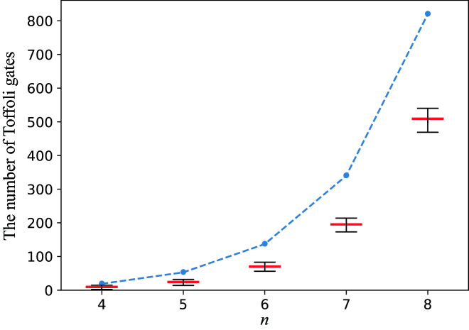
Figure 6: Quality bounds on size reduction of $n$-bit permutations (Eq. (4.53)) joined by dashed lines, and the statistical averages of the output qualities denoted by the red bars for 1000 randomly generated instances for each $n$ with depth-1 partial search. Min-Max values are also marked with black bars.

Since the number of remaining relevant row numbers decreases as the iteration goes, it becomes even easier to do the searching for larger search depth in later iterations. Let $r(i)$ denote the number of remaining relevant row numbers in normal positions at $i$-th iteration. Let $d_{j}$ be a search depth at $i$-th iteration such that $2^{j-1}<r(i)\leq 2^{j}$. In constructing and allocating even blocks, we may apply depth-$d_{j}$ partial search. In early stages, one should set small $d_{j}$ and let $d(i)=d_{j}$ so that the searching is tractable, but in later stages of left-allocating even blocks, $d_{j}$ can be larger. Similar search depth can be defined for odd blocks, and we use the same symbol $d_{j}$ for either cases. In our code, we basically set $d(i)=d_{j}$ and let users control $d_{j}$ as external parameters for each $j\in\{1,\ldots,n\}$, except $d(i)$ for $i\geq 2^{n-1}-9$. When $d_{j}$ is set as a constant $d$ for all $j$, we simply say depth-$d$ partial search is applied.

Reversible logic circuits for known hard benchmark functions [24, 17] have been synthesized by the algorithm, which are summarized in Table 1. Depth-2 partial search option is applied to the functions. Benchmark results with different $d_{j}$ options are to be posted on [1].

Table 2: Comparison of different circuit designs for AES S-box given in [13] and a circuit obtained by the algorithm with depth-4 partial search. OP and IP in the second column stand for out-of-place and in-place, and the third to the sixth columns read the number of CNOT gates, single qubit Clifford gates, T gates, and measurements. TD and W mean T-depth and the number of logical qubits, respectively.

Source	Type	#CX	#1qC	#T	#M	TD	W
[10]	OP	8683	1023	3854	0	217	44
[15]	OP	818	264	164	41	35	41
[13]	OP	654	184	136	34	6	137
This work	IP	12466	1787	5089	0	579	15

The algorithm is applied to find reversible circuits for cryptographic S-boxes. Among various S-boxes, one that has attracted the most attention from the research community is undoubtedly AES S-box. See, previous works [10, 13, 15, 36] and related references therein. Table 1 in Jaques et al.’s work [13] neatly summarizes a few notable circuit designs from the literature, and we add one more entry to it as in Table 2 with the same Q# options being used as the first entry. The design we have added in the table is first obtained by the algorithm proposed, and then it went through manual optimizations [3, 12] before Q# estimates the resources. A detailed circuit can be found in [1]. Note that we could get an even smaller T-depth at the cost of increasing the number of measurements, but we post the one without any measurements. Here we would point out that our design works in-place [8] meaning that it does not need extra bits for writing the outputs. In-place design of the S-box likely leads to a quantum oracle with a minimal number of qubits, but we leave the task of constructing an oracle as one of the future directions to explore. Note however that in Grover’s algorithm it is generally more important to optimize depth than width considering the quadratic speedup [11, 35, 14].

Efficient reversible circuits can be found for S-boxes with algebraic structures, but if an S-box does not have apparent structure, Algorithm 4 can be a good candidate for a solution. We have applied the algorithm to Skipjack [22], KHAZAD [4], and DES S-boxes [20], all of which are known not to have efficient classical implementations other than lookup tables. The results are summarized in Table 3, and the circuits can be found from [1]. To our knowledge, none of them have been analyzed before possibly due to the difficulty of handling unstructured permutation maps. Note that the algorithm is generally applicable to any substitution maps with not too large $n$, giving rise to in-place logic circuits.

Table 3: Costs of reversible circuits for various S-boxes with no structure, obtained by the algorithm with depth-3 partial search. DES has eight different S-boxes, where each takes as input a 6-bit string and outputs a 4-bit string. Two bits of garbage are unavoidable in the reversible implementation of DES S-box.

S-box	#in	#out	#grb	QC	#TOF
Skipjack	8	8	0	5440	771
KHAZAD	8	8	0	5126	742
DES-1	6	4	2	721	95
DES-2	6	4	2	672	92
DES-3	6	4	2	731	104
DES-4	6	4	2	684	94
DES-5	6	4	2	739	101
DES-6	6	4	2	794	112
DES-7	6	4	2	718	101
DES-8	6	4	2	744	100

References

- [1] Algorithm Implementation, https://github.com/ReversibleLogicCircuit/SizeReduction.
- [2] Arabzadeh, Mona and Saeedi, Mehdi, RCViewer+, version 2.5, 2013. http://ceit.aut.ac.ir/QDA/RCV.htm.
- [3] A. Barenco, C. H. Bennett, R. Cleve, D. P. DiVincenzo, N. Margolus, P. Shor, T. Sleator, J. A. Smolin, and H. Weinfurter, Elementary Gates for Quantum Computation, Phys. Rev. A, 52 (1995), pp. 3457–3467.
- [4] P. Barreto and V. Rijmen, The Khazad Legacy-Level Block Cipher, vol. 97, 2000.
- [5] S. Bravyi, T. J. Yoder, and D. Maslov, Efficient Ancilla-Free Reversible and Quantum Circuits for the Hidden Weighted Bit Function, arXiv preprint, (2020).
- [6] R. Bryant, On the Complexity of VLSI Implementations and Graph Representations of Boolean Functions with Application to Integer Multiplication, IEEE Transactions on Computers, 40 (1991), pp. 205–213.
- [7] W. J. Dally and B. P. Towles, Principles and Practices of Interconnection Networks, Morgan Kaufmann Publishers Inc., San Francisco, CA, USA, 2004.
- [8] T. G. Draper, S. A. Kutin, E. M. Rains, and K. M. Svore, A Logarithmic-Depth Quantum Carry-Lookahead Adder, Quantum Info. Comput., 6 (2006), p. 351–369.
- [9] O. Golubitsky, S. M. Falconer, and D. Maslov, Synthesis of the Optimal 4-bit Reversible Circuits, in Design Automation Conference, 2010, pp. 653–656.
- [10] M. Grassl, B. Langenberg, M. Roetteler, and R. Steinwandt, Applying Grover’s Algorithm to AES: Quantum Resource Estimates, in PQCrypto 2016, 2016, pp. 29–43.
- [11] L. K. Grover, Quantum Mechanics Helps in Searching for a Needle in a Haystack, Phys. Rev. Lett., 79 (1997), pp. 325–328.
- [12] Y. He, M.-X. Luo, E. Zhang, H.-K. Wang, and X.-F. Wang, Decompositions of n-Qubit Toffoli Gates with Linear Circuit Complexity, International Journal of Theoretical Physics, 56 (2017), pp. 2350–2361.
- [13] S. Jaques, M. Naehrig, M. Roetteler, and F. Virdia, Implementing Grover Oracles for Quantum Key Search on AES and LowMC, in Advances in Cryptology – EUROCRYPT 2020, A. Canteaut and Y. Ishai, eds., Cham, 2020, Springer International Publishing, pp. 280–310.
- [14] P. Kim, D. Han, and K. C. Jeong, Time-Space Complexity of Quantum Search Algorithms in Symmetric Cryptanalysis: Applying to AES and SHA-2, Quantum Information Processing, 17 (2018), p. 339.
- [15] B. Langenberg, H. Pham, and R. Steinwandt, Reducing the Cost of Implementing the Advanced Encryption Standard as a Quantum Circuit, IEEE Transactions on Quantum Engineering, 1 (2020), pp. 1–12.
- [16] Z. Li, H. Chen, B. Xu, X. Song, and X. Xue, An Algorithm for Synthesis of Optimal 3-qubit Reversible Circuits Based on Bit Operation, in 2008 Second International Conference on Genetic and Evolutionary Computing, 2008, pp. 455–458.
- [17] Maslov, Dmitri, Reversible Logic Synthesis Benchmarks Page. http://webhome.cs.uvic.ca/%7Edmaslov/.
- [18] D. M. Miller, D. Maslov, and G. W. Dueck, A Transformation Based Algorithm for Reversible Logic Synthesis, in Proceedings of the 40th Annual Design Automation Conference, DAC ’03, New York, NY, USA, 2003, Association for Computing Machinery, p. 318–323.
- [19] M. Möttönen, J. J. Vartiainen, V. Bergholm, and M. M. Salomaa, Quantum Circuits for General Multiqubit Gates, Phys. Rev. Lett., 93 (2004), p. 130502.
- [20] National Bureau of Standards, Data Encryption Standard, no. 46, 1977.
- [21] M. A. Nielsen and I. L. Chuang, Quantum Computation and Quantum Information: 10th Anniversary Edition, Cambridge University Press, 2010.
- [22] NIST, Skipjack and KEA Algorithm Specifications, Version 2.0, May 1998.
- [23] NIST, Advanced Encryption Standard, FIPS PUB 197, 2001.
- [24] RevLib, An Online Resources for Reversible Functions and Circuits. http://www.revlib.org/index.php.
- [25] M. Saeedi, QDA Reversible Benchmarks, 2008. http://ceit.aut.ac.ir/qda/benchmarks.htm.
- [26] M. Saeedi, M. Arabzadeh, M. S. Zamani, and M. Sedighi, Block-Based Quantum-Logic Synthesis, Quantum Info. Comput., 11 (2011), p. 262–277.
- [27] M. Saeedi and I. L. Markov, Synthesis and Optimization of Reversible Circuits— a Survey, 45 (2013).
- [28] M. Saeedi, M. S. Zamani, M. Sedighi, and Z. Sasanian, Reversible Circuit Synthesis Using a Cycle-Based Approach, J. Emerg. Technol. Comput. Syst., 6 (2010).
- [29] Saeedi, Mehdi and Zamani, Morteza Saheb and Sedighi, Mehdi and Sasanian, Zahra, Synthesis of Reversible Circuit Using Cycle-Based Approach, J. Emerg. Technol. Comput. Syst, 6 (2010), p. 13.
- [30] A. Shafaei, M. Saeedi, and M. Pedram, Reversible Logic Synthesis of k-input, m-output Lookup Tables, in 2013 Design, Automation Test in Europe Conference Exhibition (DATE), 2013, pp. 1235–1240.
- [31] T. Toffoli, Reversible Computing, in Automata, Languages and Programming, J. de Bakker and J. van Leeuwen, eds., Berlin, Heidelberg, 1980, Springer Berlin Heidelberg, pp. 632–644.
- [32] G. F. Viamontes, I. L. Markov, and J. P. Hayes, Quantum Circuit Simulation, Springer Publishing Company, 2009.
- [33] D. Zakablukov, Application of Permutation Group Theory in Reversible Logic Synthesis, CoRR, abs/1507.04309 (2015).
- [34] D. V. Zakablukov, Application of Permutation Group Theory in Reversible Logic Synthesis, Cham, 2016, Springer International Publishing, pp. 223–238.
- [35] C. Zalka, Using Grover’s Quantum Algorithm for Searching Actual Databases, Phys. Rev. A, 62 (2000), p. 052305.
- [36] J. Zou, Z. Wei, S. Sun, X. Liu, and W. Wu, Quantum Circuit Implementations of AES with Fewer Qubits, in Advances in Cryptology – ASIACRYPT 2020, S. Moriai and H. Wang, eds., Cham, 2020, Springer International Publishing, pp. 697–726.