JPGNet: Joint Predictive Filtering and Generative Network
for Image Inpainting

Abstract.

Image inpainting aims to restore the missing regions of corrupted images and make the recovery result identical to the originally complete image, which is different from the common generative task emphasizing the naturalness or realism of generated images. Nevertheless, existing works usually regard it as a pure generation problem and employ cutting-edge deep generative techniques to address it. The generative networks can fill the main missing parts with realistic contents but usually distort the local structures or introduce obvious artifacts. In this paper, for the first time, we formulate image inpainting as a mix of two problems, i.e., predictive filtering and deep generation. Predictive filtering is good at preserving local structures and removing artifacts but falls short to complete the large missing regions. The deep generative network can fill the numerous missing pixels based on the understanding of the whole scene but hardly restores the details identical to the original ones. To make use of their respective advantages, we propose the joint predictive filtering and generative network (JPGNet) that contains three branches: predictive filtering & uncertainty network (PFUNet), deep generative network, and uncertainty-aware fusion network (UAFNet). The PFUNet can adaptively predict pixel-wise kernels for filtering-based inpainting according to the input image and output an uncertainty map. This map indicates the pixels should be processed by filtering or generative networks, which is further fed to the UAFNet for a smart combination between filtering and generative results. Note that, our method as a novel framework for the image inpainting problem can benefit any existing generation-based methods. We validate our method on three public datasets, i.e., Dunhuang, Places2, and CelebA, and demonstrate that our method can enhance three state-of-the-art generative methods (i.e., StructFlow, EdgeConnect, and RFRNet) significantly with slightly extra time costs. We have released the code at https://github.com/tsingqguo/jpgnet.

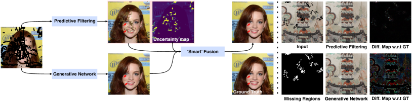
Figure 1. Left: overview of the proposed inpainting framework. Predictive filtering is able to recover the local structures (e.g., the girl’s eye and mouth) while the generative network (e.g., RFRNet (Li et al., 2020)) is good at filling large missing regions according to the understanding of the whole face. Our method takes their respective advantages, preserving the local structure and filling all missing parts naturally. Right: An example of completing the mural image from Mogao Grottoes, Dunhuang (Yu et al., 2019), China via the predictive filtering and another generative network (i.e., StructFlow (Ren et al., 2019)). Although the results of both methods look the same with the ground truth, the generative network may change the intensity of unmissed pixels according to the difference map between the prediction results and ground truth. In contrast, predictive filtering only makes changes around the missing regions. Note that, under the mural restoration task, the fidelity to the ground truth is significantly important.

1. Introduction

Image inpainting is to restore the missing or damaged areas in an image (Bertalmio et al., 2000; Guillemot and Le Meur, 2013), and it has been widely studied in computer vision and computer graphics communities long before this wave of deep generative modeling of the images. There have been numerous applications involving image inpainting such as restoring images from text overlays (Modha and Dave, 2014), occlusion removal for biometrics applications (Juefei-Xu and Savvides, 2016; Juefei-Xu et al., 2014; Juefei-Xu, 2018; Juefei-Xu et al., 2018; Abiantun et al., 2019), object removal or replacement (Criminisi et al., 2004), high-realisticity photo editing (Richard and Chang, 2001) using e.g., Photoshop, etc. Image inpainting itself is a hard problem due to fact that it is ill-posed and does not have a unique solution for any particular inpainting problem, i.e., the infamous one-to-many setting. To this end, priors and/or image-specific assumptions need to be introduced to regulate the solutions.

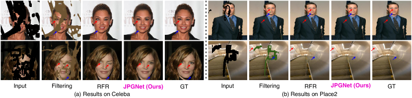
Figure 2. Visualization results of predictive filtering, deep generative network, and joint predictive filtering and generative network (JPGNet) on the CelebA and Place2 datasets. We set the deep generative network as the state-of-the-art method, i.e., RFRNet (Li et al., 2020). The red arrows show the advantages of predictive filtering for handling small missing regions and recovering local structures. The blue arrows present that generative network is good at filling large missing regions. The final results show that the proposed JPGNet share both advantages without the texture artifacts in RFRNet.

In recent years, deep generative image modeling approaches such as generative adversarial networks (GAN) variants (Yu et al., 2018; Juefei-Xu et al., 2018) as well as variational autoencoder (VEA) variants (Yeh et al., 2017; Peng et al., 2021), autoregressive variants (Oord et al., 2016; Salimans et al., 2017), etc., have shown strong performance on the image inpainting problem. These deep generative approaches can learn from a large-scale image corpus and produce novel images that share the similar image distribution as the ones in the training dataset. This strong capability of generating novel images, when conditioned upon some visible regions in the image, naturally gives solutions to the image inpainting problems. Perhaps the most impressive advantage of deep generative approaches is that they are good at dealing with large missing area image inpainting problem because they are originally intended for generating an entire image. Nevertheless, image inpainting is actually an image restoration problem, rather than a pure image generation task. The latter one only cares about whether the generated image is realistic or natural while the former one requires that the recovered regions to be identical to the true ones. Such differences make the state-of-the-art generative network-based methods less perfect for image inpainting task since they may inpaint realistic but less faithful results. For example, even the state-of-the-art method, e.g., RFRNet (Li et al., 2020), can produce distorted local structures (See Fig. 1). Moreover, some real-world applications, e.g., mural restoration (Yu et al., 2019), mainly focus on the recovery fidelity instead of the naturalness. Nevertheless, the generative network-based method (e.g., StructFlow (Ren et al., 2019)) modifies the unmissed pixels significantly (See Right subfigure in Fig. 1) although it also leads to naturally-looking inpainting result.

On a parallel track, deep predictive filtering approaches have showcased its effectiveness on various restoration tasks such as denoising (Bako et al., 2017; Mildenhall et al., 2018; Guo et al., 2013), deraining (Guo et al., 2021), and shadow removal (Fu et al., 2021). The key idea is to generate pixel-wise kernels via a deep CNN, which are then used to guide the reconstruction of each pixel with the support of its neighboring pixels. The main advantage of predictive filtering is that it respects the main information of the input, meeting the high fidelity requirements of the image inpainting. Nevertheless, it falls short to generate missing pixels from nothing or where there is not sufficient nearby pixels to extract information from. To this date, the use of deep predictive filtering for the task of image inpainting has not been explored yet.

In this paper, for the first time, we take the best of both worlds and formulate image inpainting as a mix of two problems, i.e., predictive filtering and deep generation. Predictive filtering is good at preserving local structures and removing artifacts but falls short to complete the large missing regions. The deep generative network, as discussed above, can fill the numerous missing pixels based on the understanding of the whole scene but hardly restores the details identical to the original ones. To make use of their respective advantages, we propose the joint predictive filtering and generative network (JPGNet) that contains three branches: predictive filtering & uncertainty network (PFUNet), deep generative network, and uncertainty-aware fusion network (UAFNet). The PFUNet can adaptively predict pixel-wise kernels for filtering-based inpainting according to the input image and output an uncertainty map. This map indicates the pixels should be processed by filtering or generative networks, which is further fed to the UAFNet for a smart combination between filtering and generative results. Note that, our method as a novel framework for the image inpainting problem can benefit any existing generation-based methods. We validate our method on three public datasets, i.e., Dunhuang, Places2, and CelebA, and demonstrate that our method can enhance three state-of-the-art generative methods (i.e., StructFlow, EdgeConnect, and RFRNet) significantly with slightly extra time cost.

2. Related Work

2.1. Generative Network for Image Inpainting

In recent years, deep neural network (DNN)-based approaches have displayed a promising performance in the image inpainting field (Elharrouss et al., 2020). The early work (Pathak et al., 2016) trained a CNN for completing large holes though context encoders. Then, the method (Iizuka et al., 2017) introduced the globally and locally consistent for image completion through both global and local discriminators as adversarial losses. The global discriminator assesses whether the completed image is coherent as a whole, while the local discriminator focuses on a small area centered at the generated region to enforce the local consistency. Meanwhile, there have been several studies focusing on generative face inpainting. Specifically, Yu et al. (Yu et al., 2018) found that convolutional neural networks are less effective in building long-term correlations for image inpainting. To solve this problem, they proposed contextual attention to borrow features from remote regions. Liu et al. (Liu et al., 2018a) observed that the substituting pixels in the masked holes of the inputs might introduce artifacts to the final results, and they proposed the partial convolution to force the network to use valid pixels only. Nazeri et al. (Nazeri et al., 2019) designed a two-stage adversarial model comprising an edge generator followed by an image completion network. The edge generator hallucinates edges of the missing region of the image, and the image completion network fills in the missing regions using hallucinated edges as a prior. Ren (Ren et al., 2019) also split the inpainting task into two stages, i.e., structure re-construction and texture generation. The first stage completes the missing structures of the inputs. In the second stage, a texture generator yields image details based on the reconstructed structures. More recently, Li (Li et al., 2020) proposed to recurrently infer the hole boundaries of the convolutional feature maps and use them as clues for further inference. The module progressively strengthens the constraints for the hole center and the results become explicit.

Although presenting impressive inpainting results, above works usually regard the image inpainting as a pure generation problem and employ cutting-edge deep generative techniques to address it, which can fill the main missing parts with realistic contents but might fail to get a high identity to the original one. As shown in Fig. 1, the state-of-the-art deep generative networks, i.e., RFRNet (Li et al., 2020) and StructFlow (Ren et al., 2019), might change the local structures or the pixel intensities, making the inpainting images showing obvious difference w.r.t. to ground truth. In this work, for the first time, we formulate the image inpaint as a mix of two tasks, i.e., predictive filtering and deep generation. By taking their respective advantages, our method can not only recover the local structures but also fill all missing parts naturally.

2.2. Background-aware Image Inpainting

A typical idea for image inpainting is to find suitable patches in unmissed regions to fill the hole. The key problem is how to get related patches and how to complete missing regions in a natural way (Barnes et al., 2009). Ružić and Pižurica (Ružić and Pižurica, 2015) searched the well-matched patch via Markov random filed. Jin et al. (Jin and Ye, 2015) and Guo et al. (Guo et al., 2017) utilized the low rank theory for patch searching and filling. Kawai et al. (Kawai et al., 2015) selected patches according to the object and search around background for inpainting. Liu et al. (Liu et al., 2018b) utilized the structure constraint via homograph transformation for effective inpainting. Xue et al. (Xue et al., 2017) studied the depth-based inpainting problem via the low rank. Ding et al. (Ding et al., 2019) proposed to fill missing regions via the non-local texture matching and nonlinear filtering. In this paper, we also employ the filtering for inpainting that utilizes the missing pixels’ neighboring pixels for reconstruction. In contrast to (Ding et al., 2019), our filters are pixel-wise and estimated in a one-step way via a pre-trained encoder-decoder, which is able to adapt to different inputs and regions efficiently. To best of our knowledge, this is the first attempt to adapt the deep predictive filtering for image inpainting.

2.3. Predictive Filtering for Image Restoration

Deep predictive filtering is a recently proposed DNN framework for image processing (Bako et al., 2017; Mildenhall et al., 2018, 2018; Guo et al., 2021; Brooks and Barron, 2019; Guo et al., 2020; Fu et al., 2021; Cheng et al., 2020; Zhai et al., 2020). It is basic idea is to predict the kernels for all pixels via a pre-trained deep network and use the kernels to conduce pixel-wise image filtering. Bako et al. (Bako et al., 2017) and Mildenhall et al. (Mildenhall et al., 2018) used the predictive filtering for denoising. Guo et al. (Guo et al., 2021) extended it to the field of deraining while Fu et al. (Fu et al., 2021) regarded it as a tool for fusing multiple exposure images to realize efficient shadow removal. In addition to image restoration problem, Brooks et al. (Brooks and Barron, 2019) and Guo et al. (Guo et al., 2020) employ the predictive filtering for synthesizing the motion blur. In contrast to the degradation like noise, rain streaks, and shadow, the holes (i.e., missing regions) make the image information totally lost. Intuitively, the small holes or the missing pixels at the boundary of a big hole can be reconstructed by their neighboring pixels. Nevertheless, the pixels at the center of the large hole could have diverse possibility and cannot be recovered from the neighboring pixels. These pixels should be ‘guessed’ by understanding the whole scene. Hence, it is difficult to achieve high performance for image inpainting via the naive implementation of predictive filtering. In this work, in contrast to existing predictive filtering-based restoration methods, we propose to combine it with the generative network via a new design fusion network.

3. Intuitive Discussion

Given an image $\mathbf{I}\in\mathds{R}^{H\times W}$ whose partial pixels are missed, we aim to fill these regions with realistic contents and make the processed image identical to the originally completed counterpart (i.e., the ground truth of image inpainting) denoted as $\mathbf{I}^{*}\in\mathds{R}^{H\times W}$. In this section, we first introduce two solutions for image inpainting, i.e., predictive filtering and generative network. Then, we provide some intuitive comparisons between these two solutions, driving the motivation of this work.

3.1. Predictive Filtering for Image Inpainting

Predictive filtering is an advanced image filtering technology that combines the advantages of the classical image filtering and deep learning and has been validated on various tasks, e.g., image denoising (Bako et al., 2017; Mildenhall et al., 2018), deraining (Guo et al., 2021), shadow-removal (Fu et al., 2021), and blurring (Guo et al., 2020). Its basic pipeline is to filter image with pixel-wise kernels predicted from a deep convolutional neural network (CNN). Note that, to best of our knowledge, this is the very first attempt to formulate the image inpainting as a predictive filtering problem.

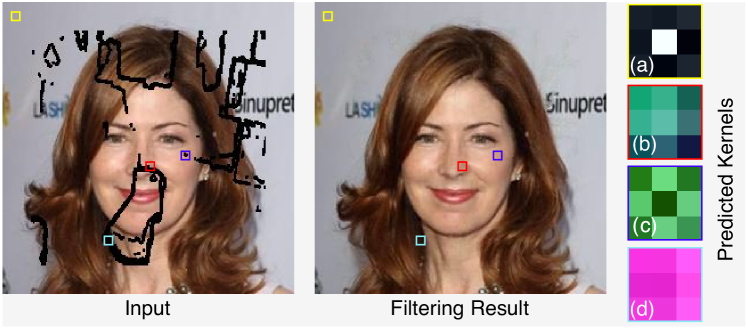
Figure 3. Predicted kernels for different pixels. Clearly, the kernels’ patterns are related to the missing regions, directly.

Specifically, given the input corrupted image $\mathbf{I}$, we process it with pixel-wise kernels by

(1) $$\hat{\mathbf{I}}_{1}(\mathbf{p})=\sum_{\mathbf{q}\in\mathcal{N}_{\mathbf{p}}}\mathbf{K}_{p}(\mathbf{q}-\mathbf{p})\mathbf{I}(\mathbf{q}),$$

where $\mathbf{p}$ and $\mathbf{q}$ represent the pixel coordinates, $\mathcal{N}_{\mathbf{p}}$ denotes the set of neighboring pixels of $\mathbf{p}$, and $\mathbf{K}_{p}\in\mathds{R}^{K\times K}$ is the exclusive kernel for pixel $\mathbf{p}$ with its kernel size being $K$. Intuitively, Eq. (1) is to reconstruct the pixel $\mathbf{p}$ with its neighboring pixels in $\mathcal{N}_{\mathbf{p}}$ and the kernel $\mathbf{K}_{p}(\mathbf{q}-\mathbf{p})$ determines the combination weight on the pixel $\mathbf{q}$. The size of $\mathcal{N}_{\mathbf{p}}$ is $K^{2}$. Different from the traditional image filtering methods (e.g., Sobel) using fixed kernels for all pixels, the predictive filtering employs a deep CNN to adaptively predict the pixel-wise kernels according to the input:

(2) $$\mathbf{K}=\text{UNet1}(\mathbf{I}),$$

where $\mathbf{K}\in\mathds{R}^{H\times W\times K^{2}}$ contains the kernels of all pixels, i.e., $\{\mathbf{K}_{p}\}$ while $\text{UNet1}(\cdot)$ is an UNet architecture (Guo et al., 2021). We can train the network with image quality related loss functions, e.g., $L_{1}$ and SSIM loss functions. As the results shown in the Fig. 2, the predictive filtering method is able to fill the small regions accurately but fails to predict the large missing patches. This is reasonable since the filtering is to reconstruct the missing pixel according to its neighbors while the large missing patches should be filled through the capability of understanding the whole scene.

3.2. Generative Network for Image Inpainting

With the rapid development of deep generative networks, state-of-the-art methods design novel generative networks (Nazeri et al., 2019; Ren et al., 2019) to map the input degraded images to the completed counterparts directly. They usually train their models with the adversarial loss function. Such methods are able to reason the large missing regions since the pre-trained deep generative models can deeply understand the scene in the degraded image and inject the prior information into the miss regions. Nevertheless, these generative models are less effective on filling small regions, which may generate new structures that are not identical to the completed counterpart. As shown in the first case of Fig. 2, the generative method leads to distorted faces, making inpainting results not like the ground truth.

3.3. Observations and Motivations

Observations. We use the predictive filtering in Sec. 3.1 and a state-of-the-art deep generative network, i.e., RFRNet (Li et al., 2020), to conduct the inpainting, respectively. We show visualization results on the CelebA and Place2 datasets in Fig. 2 and observe that: ❶ the predictive filtering is able to recover the small missing structures effectively while the generative network is ease to distort them or introduces artifacts. As shown in the results on CelebA, the predictive filtering can recover the missing eyes that have similar structure (See the opening status and eyeball position) with the ground truth. In contrast, the generative network makes the opening eyes become close and normal eyes be distorted. We have similar observations on the Place2. ❷ The deep generative network is able to fill all missing pixels while the filtering fails on the large missing regions. ❸ The RFRNet has obvious artifacts on the generated regions while the filtering results look clear on restored regions.

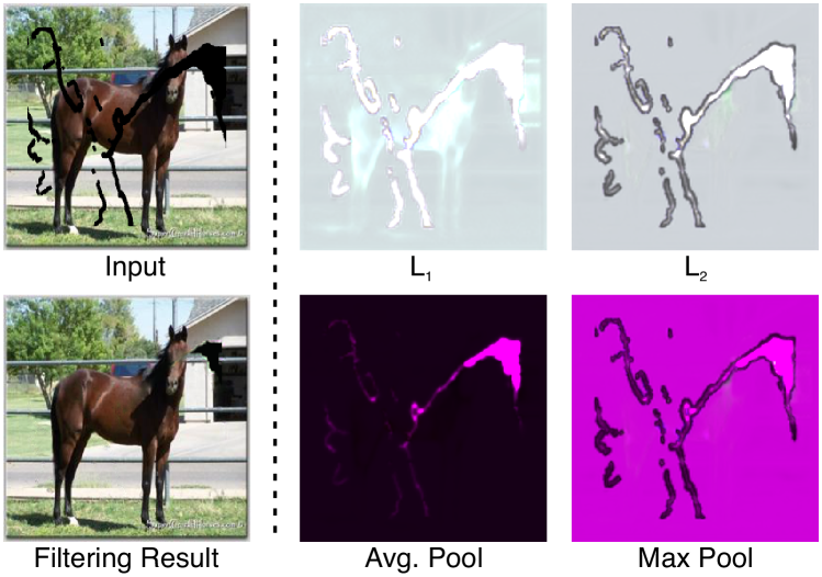
Figure 4. Uncertainty maps based on average pool, max pool, $L_{1}$, and $L_{2}$. We visualize the input and filtering results, showing that the map based on average pool can indicate whether the pixels could be recovered via the filtering.

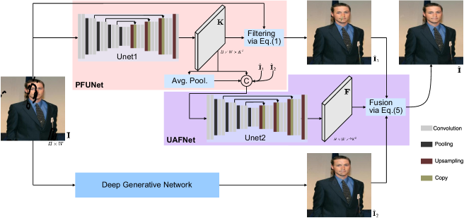
Figure 5. Overview of the joint predictive filtering and generative network (JPGNet) containing three modules, i.e., predictive filtering & uncertainty network (PFUNet), deep generative network, and uncertainty-aware fusion network. The ‘ⓒ’ denotes the concatenation layer. The ‘Avg. Pool.’ represents the averaging pooling along the channel dimension of $\mathbf{K}$, outputting the uncertainty map.

Motivations and Challenges. Clearly, above two solutions have their respective advantages and disadvantages. To let the inpainting be able to restore the small structures while reasoning large missing regions, it is better to make a combination and solve two major issues: ❶ how to identify the regions that can be reconstructed by filtering or generative networks? ❷ how to fuse the results of filtering and generation in a ‘smart’ way ? For the first challenge, we propose the predictive filtering & uncertainty network by extending the predictive filtering without extra costs. It empowers the naive predictive filtering to estimate an uncertainty map which assigns each pixel a score indicating whether the pixel can be or need to be reconstructed by filtering. For the second challenge, we propose the uncertainty-aware fusion network that can fuse the results of predictive filtering and generative network. We will detail the whole framework and contributions in Sec. 4.

4. Joint Predictive Filtering and
Generative Network

4.1. Overview

The proposed method contains three modules, i.e., predictive filtering & uncertainty network (PFUNet), deep generative network (DGNet), and uncertainty-aware fusion network (UAFNet). Intuitively, given a corrupted image $\mathbf{I}$, we feed it to the PFUNet and deep generative network, respectively, and we get two initial inpainting results, i.e., $\hat{\mathbf{I}}_{1}$ and $\hat{\mathbf{I}}_{2}$. Note that, the PFUNet also outputs an uncertainty map $\mathbf{U}$ according to the predicted filters, which assigns each pixel a score indicating whether the pixel can be or need to be reconstructed by filtering. Then, we concatenate the uncertainty map, predicted kernels, and initial restored images and feed them into the UAFNet to guide the fusion of $\hat{\mathbf{I}}_{1}$ and $\hat{\mathbf{I}}_{2}$, leading to the final result $\hat{\mathbf{I}}$ . Please refer to Fig. 5 for understanding the whole pipeline easily. Note that, our method can help any generative inpainting methods by setting them as the deep generative network in our framework. In the following, we detail the PFUNet and UAFNet, respectively.

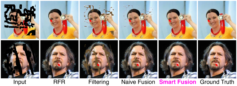
Figure 6. Two examples from CelebA dataset with the inpainting results of the deep generative network (e.g., RFRNet), predictive filtering, naive fusion via Eq. (4), and smart fusion via UAFNet in Sec. 4.3.

4.2. Predictive filtering & uncertainty network

In this section, we first rethink the predictive filtering in Sec. 3 to understand the functionality of predicted kernels, inspiring how to construct an uncertainty map indicating whether a pixel could be reconstructed by neighboring pixels.

Rethinking the functionality of pixel-wise kernels. Considering the filtering function in Eq. (1), we have the following inferences: ❶ when the pixel $\mathbf{p}$ in the input image is not missed, its kernel (i.e., $\mathbf{K}_{p}$) should be specified as

(3) $$\mathbf{K}_{p}(\mathbf{q}-\mathbf{p})=\left\{\begin{matrix}1,~{}\text{if}~{}\mathbf{q}-\mathbf{p}=[\frac{K-1}{2},\frac{K-1}{2}],\\ 0,\quad\quad\quad\quad\quad\text{otherwise}.\end{matrix}\right.$$

to make sure the $\hat{\mathbf{I}}(\mathbf{p})=\mathbf{I}(\mathbf{p})$ (See the kernel (a) in Fig. 3). ❷ when the pixel $\mathbf{p}$ at the boundary of the missing regions, its kernel is definitely different from the one in Eq. (3) and is related to the shape of the regions (See the (b) and (c) kernels in Fig. 3). ❸ Moreover, the kernel of the pixels near to the center of the large missing regions present uniform values, having different patterns to those of other pixels (See the kernel (d) in Fig. 3.). According to above discussion, the patterns of predicted kernels are able to represent the capability of using filtering to reconstruct the missing pixels.

Uncertainty map prediction and naive fusion. To validate above hypothesis, we consider operations including $\{\text{max pool},\\ \text{average pool},L_{1},L_{2}\}$ to process each kernel and get a score for each pixel to indicate whether this pixel could be recovered via the filtering or not. As a result, we can obtain a map that is further normalized to [0,1] and denoted as the uncertainty map $\mathbf{U}$. We show an example in Fig. 4 with four maps based on max pool, average pool, $L_{1}$, and $L_{2}$, respectively. Comparing the four maps with the filtering result, the map based on the average pool is able to represent the capability of pixel-wise filtering to reconstruct the missing pixels effectively. For example, the highlighted regions in ‘Avg. Pool’ is identical to the non-recovered or under-recovered regions in the filtering results.

Intuitively, we can use the uncertainty map to fuse the filtering and generation results (i.e., $\hat{\mathbf{I}}_{1}$ and $\hat{\mathbf{I}}_{2}$) directly, i.e.,

(4) $$\hat{\mathbf{I}}=(1-\mathbf{U})\odot\hat{\mathbf{I}}_{1}+\mathbf{U}\odot\hat{\mathbf{I}}_{2},$$

where ‘$\odot$’ denotes the element-wise multiplication. The above fusion process is to select the results of generative network or filtering as the final counterparts according to the uncertainty map. The pixels with high uncertainty values means they cannot be recovered via the filtering and rely on the deep generative network. In contrast, the pixels with low uncertainty are determined by filtering results. As the results shown in Fig. 6, the naive fusion is able to limit the distortion introduced by the deep generative network as the regions indicated by the red arrows. Nevertheless, such fusion process ignores the potential relationship across neighboring pixels, leading to a lot of remaining uncompleted regions. In the following, we train a uncertainty-aware fusion network to fuse the filtering and generation results in a ‘smart’ way.

4.3. Uncertainty-aware fusion network

Given two initial results, i.e., $\hat{\mathbf{I}}_{1}$ and $\hat{\mathbf{I}}_{2}$, we propose to fuse them by

(5) $$\hat{\mathbf{I}}(\mathbf{p})=\sum_{\mathbf{q}\in\mathcal{N}_{\mathbf{p}}}\mathbf{F}_{p}(\mathbf{q}-\mathbf{p})\odot[\hat{\mathbf{I}}_{1}(\mathbf{q}),\hat{\mathbf{I}}_{2}(\mathbf{q})],$$

where $\mathbf{p}$ and $\mathbf{q}$ are the pixel coordinates, $\mathcal{N}_{\mathbf{p}}$ denotes the set of neighboring pixels of $\mathbf{p}$. The matrix $\mathbf{F}_{p}\in\mathds{R}^{K\times K\times 2}$ contains the fusion parameters with $K^{2}$ being the size of $\mathcal{N}_{\mathbf{p}}$ and $\mathbf{F}_{p}(\mathbf{q}-\mathbf{q})$ and $[\hat{\mathbf{I}}_{1}(\mathbf{q}),\hat{\mathbf{I}}_{2}(\mathbf{p})]$ are vectors with size of $1\times 2$. Comparing with the Eq. (4), the new fusion formulation consider the neighboring pixels. Moreover, we propose to predict the parameters $\mathbf{F}_{p}$ via a network that takes the uncertainty map $\mathbf{U}$, predicted kernels $\mathbf{K}$, and the initial results (i.e., $\hat{\mathbf{I}}_{1}$ and $\hat{\mathbf{I}}_{2}$) as the inputs and outputs

(6) $$\mathbf{F}=\text{UNet2}(\mathbf{U},\mathbf{K},\hat{\mathbf{I}}_{1},\hat{\mathbf{I}}_{2}),$$

$\mathbf{F}\in\mathds{R}^{H\times W\times 2K^{2}}$. It contains all fusion parameters, i.e., $\{\mathbf{F}_{p}\}$. We will detail the network architecture in Sec. 4.4.

4.4. Implementation Details

We implement our method to enhance three state-of-the-art deep generative networks, i.e., StructFlow (Ren et al., 2019), EdgeConnect (Nazeri et al., 2019), and RFRNet (Li et al., 2020), we follow their released code and train their models according respective default setups. In the following, we introduce the details about the proposed PFUNet and UAFNet.

Network Architectures. In PFUNet and UAFNet, the UNet1 and UNet2 are their main architectures and we follow the UNet (Ronneberger et al., 2015) setups in (Guo et al., 2021). They share similar structures but have different input and output channels according to their functionalities. Please refer to Table 1 for details. Note that, in previous subsections, we formulate the method for single-channel images for better understanding. Here, we implement our method for the color images by predicting kernels or fusion parameters for each color channel independently. For example, the size of $\mathbf{K}$ and $\mathbf{F}$ becomes $3K^{2}$ and $2*3K^{2}$. We fix the kernel size $K$ as 3 since it allows efficient training.

Table 1. Architecture of UNet1 or UNet2 for PFUNet or UAFNet, respectively. The ‘Blk’ denotes a block containing three stacked convolution layers. The ‘[$\cdot$]’ denotes the concatenation operation. Each convolution layer is followed by a batch normalization layer and an activation layer. For UNet1, the input is the corrupted image $\mathbf{I}$ with $C_{\text{in}}=3$ for color image and the output is $\mathbf{K}$ with $C_{\text{o}}=3K^{2}=27$ for each pixel in each color channel has a $K\times K$ kernel. For UNet2, the input is [$\mathbf{U}$, $\mathbf{K}$, $\hat{\mathbf{I}}_{1}$, $\hat{\mathbf{I}}_{2}$] and the output is $\mathbf{F}$ with $C_{\text{o}}=2*3K^{2}$.

	input	output	output size	49-layer
Blk1	Input	$\mathbf{x}_{1}$	$256\times 256$	$3\times$ conv(3, $C_{\text{in}}$, 64)
Blk2	$\mathbf{x}_{1}$	$\mathbf{x}_{2}$	$128\times 128$	$3\times$ conv(3, 64, 128)
Blk3	$\mathbf{x}_{2}$	$\mathbf{x}_{3}$	$64\times 64$	$3\times$ conv(3, 128, 256)
Blk4	$\mathbf{x}_{3}$	$\mathbf{x}_{4}$	$32\times 32$	$3\times$ conv(3, 256, 512)
Blk5	$\mathbf{x}_{4}$	$\mathbf{x}_{5}$	$16\times 16$	$3\times$ conv(3, 512, 512)
Blk6	$\mathbf{x}_{5}$	$\mathbf{x}_{6}$	$32\times 32$	$3\times$ conv(3, 512, 512)
Blk7	[$\mathbf{x}_{6}$,$\mathbf{x}_{4}$]	$\mathbf{x}_{7}$	$64\times 64$	$3\times$ conv(3, 512, 256)
Blk8	[$\mathbf{x}_{7}$,$\mathbf{x}_{3}$]	$\mathbf{x}_{8}$	$128\times 128$	$3\times$ conv(3, 256, 27)
Conv	[$\mathbf{x}_{8}$,$\mathbf{x}_{2}$]	$\mathbf{K}$/ $\mathbf{F}$	$256\times 256$	conv(1, 27, $C_{\text{o}}$)

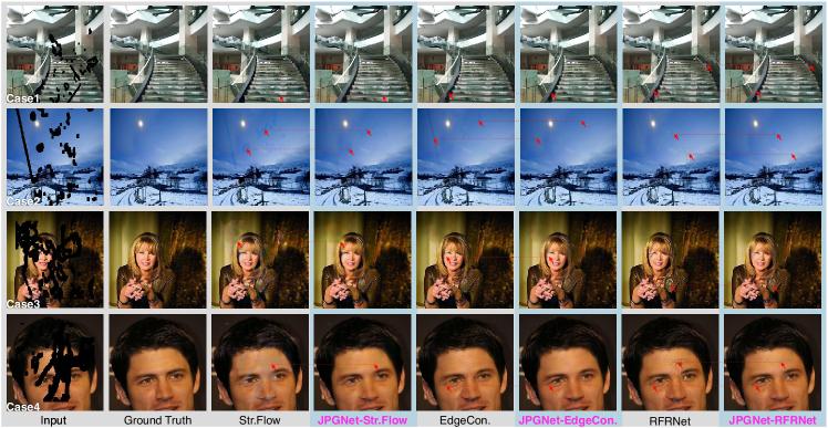
Figure 7. Four visualization results of StructFlow (Str. Flow) (Ren et al., 2019), EdgeConnect (EdgeCon.) (Nazeri et al., 2019), RFRNet (Li et al., 2020), and the JPGNet-enhanced counterparts. The first two cases are from the Place2 dataset while Case3 and Case4 stem from the CelebA dataset. We use red arrows to show the main advantages of the JPGNet.

Loss functions. We train the whole framework with two stages. First, we train the PFUNet by considering two loss functions, i.e., $L_{1}$ and SSIM loss functions. Given the estimated image $\hat{\mathbf{I}}$ and the ground truth $\mathbf{I}^{*}$, we have

(7) $$\mathcal{L}(\hat{\mathbf{I}},\mathbf{I}^{*})=\|\hat{\mathbf{I}}-\mathbf{I}^{*}\|_{1}-\lambda~{}\text{SSIM}(\hat{\mathbf{I}},\mathbf{I}^{*}),$$

where we fix $\lambda=0.2$ during training process. After training the PFUNet and the deep generative networks, we fix them and train the UAFNet through the same loss function.

Training details. We employ Adam as the optimizer with the learning rate of 0.0002. We train PFUNet for 450,000 epochs, and UAFNet for 100,000 epochs. All experiments are implemented on the same platform with a single NVIDIA Tesla V100 GPU.

5. Experimental Results

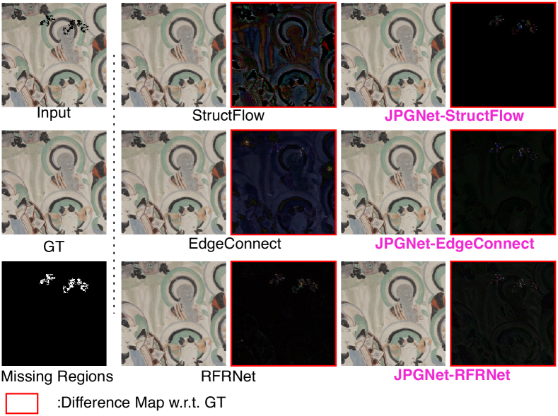
Figure 8. An example from the Dunhuang dataset. In addition to the inpainting results of six methods, we show the difference maps between the predicted results and the ground truth (GT).

5.1. Setups

Datasets. We validate the proposed method on three datasets, i.e., Places2 challenge dataset (Zhou et al., 2017), CelebA dataset (Liu et al., 2015), and Dunhuang Challenge (Yu et al., 2019). We choose the Dunhuang challenge since it is a representative application for image inpainting in the real world, i.e., that is, to automatically recover the missing regions in the paintings that are created by thousands and thousands of artists over 10 centuries. The Places2 dataset contains over eight million images captured under over 365 scenes, which is suitable for validating the methods on natural scenes. The CelebA dataset contains over 180 thousand face images, evaluating the capability of face inpainting.

Metrics. We follow the comment setups in the image inpainting and use the peak signal-to-noise ratio (PSNR) and structural similarity index (SSIM) for the restoration quality evaluation. We also provide the qualitative comparison via diverse visualization.

Mask Setups. For the Places and CelebA datasets, we use the irregular mask dataset (Liu et al., 2018a), which is also a common setup in recent works (Ren et al., 2019). Note that, the mask images are classified to three categories (i.e., $0\%-20\%$, $20\%-40\%$, $40\%-60\%$,) based on the hole sizes relative to the image size. For the Dunhuang dataset, we follow its official setup and use their synthetic method considering the real-world degradation caused by the corrosion and aging.

Baselines. We use our method to enhance three state-of-the-art inpainting methods, i.e., StructFlow (Ren et al., 2019), EdgeConnectnect (Nazeri et al., 2019), RFRNetNet (Li et al., 2020).

5.2. Comparison Results

Table 2. Comparison results on Places2, CelebA, and Dunhuang datasets.

	Datasets	Places2			CelebA			Dunhuang
	Mask Ratio	0%-20%	20%-40%	40%-60%	0%-20%	20%-40%	40%-60%	Default
PSNR	StructFlow (Ren et al., 2019)	29.039	23.111	19.421	31.618	25.283	20.829	35.199
	JPGNet-StructFlow	31.381	24.889	20.783	33.781	26.501	21.477	37.268
	EdgeConnect (Nazeri et al., 2019)	29.909	23.382	19.516	32.781	25.347	20.449	36.419
	JPGNet-EdgeConnect	31.337	24.388	20.283	34.110	26.351	21.195	37.369
	RFRNet (Li et al., 2020)	29.442	22.701	18.647	34.521	26.328	20.994	35.751
	JPGNet-RFRNet	30.834	24.056	19.954	35.898	27.639	22.089	37.646
SSIM	StructFlow (Ren et al., 2019)	0.9335	0.8180	0.6736	0.9487	0.8598	0.7417	0.9559
	JPGNet-StructFlow	0.9493	0.8489	0.7141	0.9640	0.8875	0.8025	0.9682
	EdgeConnect (Nazeri et al., 2019)	0.9398	0.8227	0.6711	0.9586	0.8689	0.7362	0.9635
	JPGNet-EdgeConnect	0.9516	0.8493	0.7114	0.9670	0.8909	0.7725	0.9718
	RFRNet (Li et al., 2020)	0.9297	0.7893	0.6156	0.9674	0.8865	0.7538	0.9616
	JPGNet-RFRNet	0.9465	0.8373	0.6937	0.9740	0.9073	0.7919	0.9686

Table 3. Ablation study results on Places2, CelebA, and Dunhuang datasets. We consider three variants, i.e., predictive filtering, JPGNet with naive fusion (N.F.) defined in Eq. (4), and JPGNet with smart fusion (S.F.) defined in Eq. (6).

	Datasets	Places2			CelebA			Dunhuang
	Mask Ratio	0%-20%	20%-40%	40%-60%	0%-20%	20%-40%	40%-60%	Default
PSNR	Input	16.376	11.271	9.127	16.259	11.051	8.887	15.897
	Predictive Filtering	25.500	17.652	13.764	26.986	18.837	14.777	37.021
	JPGNet-StructFlow-N.F.	25.580	17.665	13.795	29.189	21.551	17.603	36.703
	JGPNet-StructFlow-S.F.	31.381	24.889	20.783	33.781	26.501	21.477	37.268
	JPGNet-EdgeConnect-N.F.	25.513	17.663	13.793	29.315	21.537	17.489	37.265
	JPGNet-EdgeConnect-S.F.	31.337	24.388	20.283	34.110	26.351	21.195	37.369
	JPGNet-RFRNet-N.F.	25.510	17.659	13.764	29.375	21.537	17.489	37.217
	JPGNet-RFRNet-S.F.	30.834	24.056	19.954	35.898	27.639	22.089	37.646
SSIM	Input	0.8366	0.6069	0.4165	0.8365	0.6094	0.4226	0.7661
	Predictive Filtering	0.9180	0.7572	0.5913	0.9281	0.7804	0.6290	0.9692
	JPGNet-StructFlow-N.F.	0.9187	0.7586	0.5930	0.9338	0.7978	0.6468	0.9674
	JPGNet-StructFlow-S.F.	0.9493	0.8489	0.7141	0.9640	0.8875	0.8025	0.9701
	JPGNet-EdgeConnect-N.F.	0.9181	0.7574	0.5902	0.9352	0.7997	0.6447	0.9701
	JPGNet-EdgeConnect-S.F.	0.9516	0.8493	0.7114	0.9670	0.8909	0.7725	0.9718
	JPGNet-RFRNet-N.F.	0.9180	0.7572	0.5894	0.9358	0.8007	0.6464	0.9697
	JPGNet-RFRNet-S.F.	0.9465	0.8373	0.6937	0.9740	0.9073	0.7919	0.9723

Table 4. Average Time cost (ms) per image of JPGNet and its three modules, i.e., predictive filtering & uncertainty network (PFUNet), uncertainty-aware fusion network (UAFNet), and deep generative network (DGNet), on the three datasets. We also report the rate of each module w.r.t. the total cost.

	JPGNet-StructFlow				JPGNet-EdgeConnect				JPGNet-RFRNet
Time (ms)	PFUNet	UAFNet	DGNet	Total	PFUNet	UAFNet	DGNet	Total	PFUNet	UAFNet	DGNet	Total
Places2	4.42	3.33	30.55	38.30	4.69	3.40	15.05	23.14	3.20	3.10	15.95	22.25
Rate (%)	11.54	8.69	79.77	100.0	20.27	14.69	65.03	100.0	14.38	13.93	71.69	100.0
CelebA	4.48	3.39	30.66	38.53	4.80	3.42	15.84	24.06	3.55	3.42	17.00	23.97
Rate (%)	11.63	8.80	79.57	100.0	19.95	14.21	65.84	100.0	14.81	14.27	70.92	100.0
Dunhuang	4.88	3.51	31.26	39.65	4.62	3.37	14.97	22.96	3.32	3.33	16.78	23.43
Rate (%)	12.31	8.85	78.84	100.0	20.12	14.68	65.20	100.0	14.17	14.21	71.62	100.0

Quantitative comparison. We first compare the three deep generative networks, i.e., StructFlow (Ren et al., 2019), EdgeConnect (Nazeri et al., 2019), and RFRNetNet (Li et al., 2020), with the respective enhanced counterparts through the proposed JPGNet in Table 2. We observe that: ❶ With our JPGNet, all deep generative networks are significantly improved on all three different mask ratios and three datasets, referring that our method indeed makes up drawbacks of the generative network to let the output be more identical to the ground truth. ❷ In terms of the time cost, as shown in Table 4, our method only takes slightly more time (around 8ms) than the original deep generative networks (DGNets) (See ‘Total’ column in Table 4) due to the high-efficiency of predictive filtering (Guo et al., 2021) and smart fusion. Overall, our method is able to enhance the generative network-based inpainting methods significantly with slight extra time cost.

Qualitative comparison. We further present the visualization results for the qualitative comparison in Fig. 7. We have the following observations: ❶ JPGNet is able to remove the artifacts of deep generative networks, leading to more natural inpainting results that is more identical to the ground truth. For example, in Case2 and Case3, all of the three baseline methods show obvious artifacts, which are limited by using JPGNet. ❷ JPGNet can help the deep generative networks avoid the structure distortions. For example, in the Case1, the EdgeConnect method makes the edge of steps distorted while the JPGNet-EdgeConnect recovers the arc edge of the steps. In Case4, the EdgeConnect can fill the missing pixels while generating a natural face. Nevertheless, the generated face looks much older than the real one (i.e., ground truth). In contrast, our method can produce a more identical face to the ground truth. To further validate this, we conduct a visualization comparison on Dunhuang dataset. As shown in Fig. 8, all deep generative networks and their JPGNet counterparts can generate visually natural inpainting results that looks identical to the ground truth. Nevertheless, when we compare the difference maps between the completed images and the ground truth, we see that both EdgeConnect and StructFlow lead to obvious intensity variations across all pixels even most of them are not lost. In contrast, JPGNet-enhanced versions only have clear differences on missing regions, which further demonstrates that our method makes the results of deep generative models more identical to the ground truth.

5.3. Ablation Study

Quantitative results. We consider three variants of our method, i.e., predictive filtering in Sec. 3.1, naive fusion for joint predictive filtering and generative network in Sec. 4.2, and the proposed smart fusion based on uncertainty-aware fusion network in Sec. 4.3. We report the results in Table 3 and have the following observations: ❶ Comparing with input images’ PSNR and SSIM, predictive filtering presents obvious quality improvement, demonstrating the effectiveness of filtering for the image inpainting task. ❷ With the naive fusion strategy, the PSNR and SSIM of predictive filtering is slightly enhanced since the deep generative networks introduce more information according the whole understanding of the whole scene. ❸ The proposed smart fusion, i.e., UAFNet, presents significant improvements over the naive fusion on the combination of predictive filtering and deep generative networks. ❹ In terms of the time cost reported in Table 4, the PFUNet and UAFNet only takes around 4.5 ms and 3.4 ms per image on the three datasets, which is significantly less than the deep generative network (DGNet). As a result, JPGNet only leads to slight extra time costs.

Qualitative results. As shown in Fig. 6, the naive fusion based on the uncertainty map fills most of missing pixels but still leave some small missing regions. The UAFNet-based smart fusion can fill all missing pixels with natural appearance while recovering local structures and removing some artifacts introduced by the RFRNet.

6. Conclusion

In this paper, we have formulated the image inpainting as a mix of two problems, i.e., deep predictive image filtering and deep image generation. Predictive filtering excels at preserving local structures and removing artifacts but falls short to complete the large missing regions. The deep generative network can fill the numerous missing pixels based on the understanding of the whole scene but hardly restores the details identical to the original ones. To make use of the best of both worlds, we propose the joint predictive filtering and generative network (JPGNet) that contains three branches: predictive filtering & uncertainty network (PFUNet), deep generative network, and uncertainty-aware fusion network (UAFNet). The PFUNet can adaptively predict pixel-wise kernels for filtering-based inpainting according to the input image and output an uncertainty map. This map indicates the pixels should be processed by filtering or generative networks, which is further fed to the UAFNet for a smart combination between filtering and generative results. We have validated our method on three public datasets, i.e., Dunhuang, Places2, and CelebA, and demonstrated that our method can enhance three state-of-the-art generative methods (i.e., StructFlow, EdgeConnect, and RFRNet) significantly with slightly extra time cost.

- (1)
- Abiantun et al. (2019) Ramzi Abiantun, Felix Juefei-Xu, Utsav Prabhu, and Marios Savvides. 2019. SSR2: Sparse Signal Recovery for Single-Image Super-Resolution on Faces with Extreme Low Resolutions. Pattern Recognition (2019).
- Bako et al. (2017) Steve Bako, Thijs Vogels, Brian McWilliams, Mark Meyer, Jan Novák, Alex Harvill, Pradeep Sen, Tony DeRose, and Fabrice Rousselle. 2017. Kernel-predicting convolutional networks for denoising Monte Carlo renderings. ACM Trans. Graph. 36, 4 (2017), 97:1–97:14.
- Barnes et al. (2009) Connelly Barnes, Eli Shechtman, Adam Finkelstein, and Dan B Goldman. 2009. PatchMatch: A randomized correspondence algorithm for structural image editing. ACM Trans. Graph. 28, 3 (2009), 24.
- Bertalmio et al. (2000) Marcelo Bertalmio, Guillermo Sapiro, Vincent Caselles, and Coloma Ballester. 2000. Image inpainting. In Proceedings of the 27th annual conference on Computer graphics and interactive techniques. 417–424.
- Brooks and Barron (2019) Tim Brooks and Jonathan T Barron. 2019. Learning to synthesize motion blur. In Proceedings of the IEEE/CVF Conference on Computer Vision and Pattern Recognition. 6840–6848.
- Cheng et al. (2020) Yupeng Cheng, Felix Juefei-Xu, Qing Guo, Huazhu Fu, Xiaofei Xie, Shang-Wei Lin, Weisi Lin, and Yang Liu. 2020. Adversarial Exposure Attack on Diabetic Retinopathy Imagery. arXiv preprint arXiv:2009.09231 (2020).
- Criminisi et al. (2004) Antonio Criminisi, Patrick Pérez, and Kentaro Toyama. 2004. Region filling and object removal by exemplar-based image inpainting. IEEE Transactions on image processing 13, 9 (2004), 1200–1212.
- Ding et al. (2019) D. Ding, S. Ram, and J. J. Rodríguez. 2019. Image Inpainting Using Nonlocal Texture Matching and Nonlinear Filtering. IEEE Transactions on Image Processing 28, 4 (2019), 1705–1719.
- Elharrouss et al. (2020) Omar Elharrouss, Noor Almaadeed, Somaya Al-Maadeed, and Younes Akbari. 2020. Image Inpainting: A Review. Neural Processing Letters 51, 2 (2020), 2007–2028.
- Fu et al. (2021) Lan Fu, Changqing Zhou, Qing Guo, Felix Juefei-Xu, Hongkai Yu, Wei Feng, Yang Liu, and Song Wang. 2021. Auto-exposure Fusion for Single-image Shadow Removal. In CVPR.
- Guillemot and Le Meur (2013) Christine Guillemot and Olivier Le Meur. 2013. Image inpainting: Overview and recent advances. IEEE signal processing magazine 31, 1 (2013), 127–144.
- Guo et al. (2013) Qing Guo, Fangmin Dong, Shuifa Sun, Bangjun Lei, and Bruce Z Gao. 2013. Image denoising algorithm based on contourlet transform for optical coherence tomography heart tube image. IET image processing 7, 5 (2013), 442–450.
- Guo et al. (2017) Qiang Guo, Shanshan Gao, Xiaofeng Zhang, Yilong Yin, and Caiming Zhang. 2017. Patch-based image inpainting via two-stage low rank approximation. IEEE transactions on visualization and computer graphics 24, 6 (2017), 2023–2036.
- Guo et al. (2020) Qing Guo, Felix Juefei-Xu, Xiaofei Xie, Lei Ma, Jian Wang, Bing Yu, Wei Feng, and Yang Liu. 2020. Watch out! Motion is Blurring the Vision of Your Deep Neural Networks. Advances in Neural Information Processing Systems 33 (2020).
- Guo et al. (2021) Qing Guo, Jingyang Sun, Felix Juefei-Xu, Lei Ma, Xiaofei Xie, Wei Feng, Jianjun Zhao, and Yang Liu. 2021. EfficientDeRain: Learning Pixel-wise Dilation Filtering for High-Efficiency Single-Image Deraining. In AAAI.
- Iizuka et al. (2017) Satoshi Iizuka, Edgar Simo-Serra, and Hiroshi Ishikawa. 2017. Globally and Locally Consistent Image Completion. ACM Transactions on Graphics 36, 4 (2017), 1–14.
- Jin and Ye (2015) Kyong Hwan Jin and Jong Chul Ye. 2015. Annihilating filter-based low-rank Hankel matrix approach for image inpainting. IEEE Transactions on Image Processing 24, 11 (2015), 3498–3511.
- Juefei-Xu (2018) F. Juefei-Xu. 2018. Unconstrained Periocular Face Recognition: From Reconstructive Dictionary Learning to Generative Deep Learning and Beyond. PhD Dissertation, Carnegie Mellon University (2018).
- Juefei-Xu et al. (2018) Felix Juefei-Xu, Rahul Dey, Vishnu Naresh Bodetti, and Marios Savvides. 2018. RankGAN: A Maximum Margin Ranking GAN for Generating Faces. In Proceedings of the Asian Conference on Computer Vision (ACCV).
- Juefei-Xu et al. (2014) F. Juefei-Xu, Dipan K. Pal, and M. Savvides. 2014. Hallucinating the Full Face from the Periocular Region via Dimensionally Weighted K-SVD. In Proceedings of the IEEE Conference on Computer Vision and Pattern Recognition Workshops (CVPRW). IEEE, 1–8.
- Juefei-Xu and Savvides (2016) F. Juefei-Xu and M. Savvides. 2016. Fastfood Dictionary Learning for Periocular-Based Full Face Hallucination. In Proceedings of the IEEE Seventh International Conference on Biometrics: Theory, Applications, and Systems (BTAS). IEEE, 1–8.
- Kawai et al. (2015) Norihiko Kawai, Tomokazu Sato, and Naokazu Yokoya. 2015. Diminished reality based on image inpainting considering background geometry. IEEE transactions on visualization and computer graphics 22, 3 (2015), 1236–1247.
- Li et al. (2020) Jingyuan Li, Ning Wang, Lefei Zhang, Bo Du, and Dacheng Tao. 2020. Recurrent Feature Reasoning for Image Inpainting. In 2020 IEEE/CVF Conference on Computer Vision and Pattern Recognition (CVPR). 7757–7765.
- Liu et al. (2018a) Guilin Liu, Fitsum A Reda, Kevin J Shih, Ting-Chun Wang, Andrew Tao, and Bryan Catanzaro. 2018a. Image inpainting for irregular holes using partial convolutions. In Proceedings of the European Conference on Computer Vision (ECCV). 85–100.
- Liu et al. (2018b) Jiaying Liu, Shuai Yang, Yuming Fang, and Zongming Guo. 2018b. Structure-guided image inpainting using homography transformation. IEEE Transactions on Multimedia 20, 12 (2018), 3252–3265.
- Liu et al. (2015) Ziwei Liu, Ping Luo, Xiaogang Wang, and Xiaoou Tang. 2015. Deep learning face attributes in the wild. In Proceedings of the IEEE international conference on computer vision. 3730–3738.
- Mildenhall et al. (2018) B. Mildenhall, J. T. Barron, J. Chen, D. Sharlet, R. Ng, and R. Carroll. 2018. Burst Denoising with Kernel Prediction Networks. In CVPR. 2502–2510.
- Mildenhall et al. (2018) Ben Mildenhall, Jonathan T Barron, Jiawen Chen, Dillon Sharlet, Ren Ng, and Robert Carroll. 2018. Burst denoising with kernel prediction networks. In Proceedings of the IEEE Conference on Computer Vision and Pattern Recognition. 2502–2510.
- Modha and Dave (2014) Uday Modha and Preeti Dave. 2014. Image inpainting-automatic detection and removal of text from images. International Journal of Engineering Research and Applications (IJERA), ISSN (2014), 2248–9622.
- Nazeri et al. (2019) Kamyar Nazeri, Eric Ng, Tony Joseph, Faisal Qureshi, and Mehran Ebrahimi. 2019. EdgeConnect: Structure Guided Image Inpainting using Edge Prediction. In The IEEE International Conference on Computer Vision (ICCV) Workshops.
- Oord et al. (2016) Aaron van den Oord, Nal Kalchbrenner, Oriol Vinyals, Lasse Espeholt, Alex Graves, and Koray Kavukcuoglu. 2016. Conditional image generation with pixelcnn decoders. arXiv preprint arXiv:1606.05328 (2016).
- Pathak et al. (2016) Deepak Pathak, Philipp Krahenbuhl, Jeff Donahue, Trevor Darrell, and Alexei A. Efros. 2016. Context Encoders: Feature Learning by Inpainting. In 2016 IEEE Conference on Computer Vision and Pattern Recognition (CVPR). 2536–2544.
- Peng et al. (2021) Jialun Peng, Dong Liu, Songcen Xu, and Houqiang Li. 2021. Generating Diverse Structure for Image Inpainting With Hierarchical VQ-VAE. arXiv preprint arXiv:2103.10022 (2021).
- Ren et al. (2019) Yurui Ren, Xiaoming Yu, Ruonan Zhang, Thomas H. Li, Shan Liu, and Ge Li. 2019. StructureFlow: Image Inpainting via Structure-aware Appearance Flow. In IEEE International Conference on Computer Vision (ICCV).
- Richard and Chang (2001) MMOBB Richard and McKenna Yu-Sung Chang. 2001. Fast digital image inpainting. In Appeared in the Proceedings of the International Conference on Visualization, Imaging and Image Processing (VIIP 2001), Marbella, Spain. 106–107.
- Ronneberger et al. (2015) Olaf Ronneberger, Philipp Fischer, and Thomas Brox. 2015. U-net: Convolutional networks for biomedical image segmentation. In International Conference on Medical image computing and computer-assisted intervention. 234–241.
- Ružić and Pižurica (2015) T. Ružić and A. Pižurica. 2015. Context-Aware Patch-Based Image Inpainting Using Markov Random Field Modeling. IEEE Transactions on Image Processing 24, 1 (2015), 444–456. https://doi.org/10.1109/TIP.2014.2372479
- Salimans et al. (2017) Tim Salimans, Andrej Karpathy, Xi Chen, and Diederik P Kingma. 2017. Pixelcnn++: Improving the pixelcnn with discretized logistic mixture likelihood and other modifications. arXiv preprint arXiv:1701.05517 (2017).
- Xue et al. (2017) Hongyang Xue, Shengming Zhang, and Deng Cai. 2017. Depth image inpainting: Improving low rank matrix completion with low gradient regularization. IEEE Transactions on Image Processing 26, 9 (2017), 4311–4320.
- Yeh et al. (2017) Raymond A Yeh, Chen Chen, Teck Yian Lim, Alexander G Schwing, Mark Hasegawa-Johnson, and Minh N Do. 2017. Semantic image inpainting with deep generative models. In Proceedings of the IEEE conference on computer vision and pattern recognition. 5485–5493.
- Yu et al. (2018) Jiahui Yu, Zhe Lin, Jimei Yang, Xiaohui Shen, Xin Lu, and Thomas S Huang. 2018. Generative image inpainting with contextual attention. In Proceedings of the IEEE conference on computer vision and pattern recognition. 5505–5514.
- Yu et al. (2019) Tianxiu Yu, Shijie Zhang, Cong Lin, Shaodi You, Jian Wu, Jiawan Zhang, Xiaohong Ding, and Huili An. 2019. Dunhuang Grottoes Painting Dataset and Benchmark. arXiv preprint arXiv:1907.04589 (2019).
- Zhai et al. (2020) Liming Zhai, Felix Juefei-Xu, Qing Guo, Xiaofei Xie, Lei Ma, Wei Feng, Shengchao Qin, and Yang Liu. 2020. It’s Raining Cats or Dogs? Adversarial Rain Attack on DNN Perception. arXiv preprint arXiv:2009.09205 (2020).
- Zhou et al. (2017) Bolei Zhou, Agata Lapedriza, Aditya Khosla, Aude Oliva, and Antonio Torralba. 2017. Places: A 10 million image database for scene recognition. IEEE transactions on pattern analysis and machine intelligence 40, 6 (2017), 1452–1464.