Model order reduction for bilinear systems with non-zero initial states – different approaches with error bounds

Abstract

In this paper, we consider model order reduction for bilinear systems with non-zero initial conditions. We discuss choices of Gramians for both the homogeneous and the inhomogeneous parts of the system individually and prove how these Gramians characterize the respective dominant subspaces of each of the two subsystems. Proposing different, not necessarily structure preserving, reduced order methods for each subsystem, we establish several strategies to reduce the dimension of the full system. For all these approaches, error bounds are shown depending on the truncated Hankel singular values of the subsystems. Besides the error analysis, stability is discussed. In particular, a focus is on a new criterion for the homogeneous subsystem guaranteeing the existence of the associated Gramians and an asymptotically stable realization of the system.

Keywords: Model order reduction, bilinear systems, error bounds, stability analysis

MSC classification: 65L05, 93A15, 93C10, 93D20

1 Introduction

In this paper, we study model order reduction (MOR) techniques for the following system with non-zero initial states:

$$\dot{x}(t) =Ax(t)+Bu(t)+\sum_{k=1}^{m}N_{k}x(t)u_{k}(t),\quad x(0)=x_{0}=X_{0}v_{0},$$ (1a)

$$y(t) =Cx(t),\quad t\geq 0,$$ (1b)

where $A,N_{k}\in\mathbb{R}^{n\times n}$, $B\in\mathbb{R}^{n\times m}$, and $C\in\mathbb{R}^{p\times n}$. Moreover, $x$ is the state vector, $y$ the quantity of interest and the columns of $X_{0}\in\mathbb{R}^{n\times q}$ span all initial states $x_{0}$ that are considered here, i.e., there exist $v_{0}\in\mathbb{R}^{q}$ such that $x_{0}=X_{0}v_{0}$. We assume that the matrix $A$ is Hurwitz, meaning that $\sigma(A)\subset\mathbb{C}_{-}=\{z\in\mathbb{C}:\quad\Re(z)<0\}$, where $\sigma(\cdot)$ denotes the spectrum of a matrix and $\Re(\cdot)$ represents the real part of a complex number. Furthermore, let $u=(\begin{matrix}u_{1},u_{2},\dots,u_{m}\end{matrix})^{\top}\in L^{2}$, i.e.,

$$\left\|u\right\|_{L^{2}}^{2}:=\int_{0}^{\infty}\left\|u(s)\right\|^{2}_{2}ds=\int_{0}^{\infty}u^{\top}(s)u(s)ds<\infty.$$

There exist many different MOR techniques for bilinear systems when $x_{0}=0$, e.g., methods that are balancing related (Al-Baiyat  Bettayeb, 1993; Hartmann ., 2013; Redmann, 2018, 20201), optimization/interpolation based (Benner  Breiten, 2012; Flagg  Gugercin, 2015) and data-driven (Antoulas ., 2016). However, many applications involve non-zero initial states such that a study for MOR for (1) is essential. Several approaches in this context have been established for linear systems (Bauer ., 2014; Beattie ., 2017; Daragmeh ., 2019; Heinkenschloss ., 2011; Schröder  Voigt, 2020). There is no straightforward generalization of these techniques to (1), since the study of transfer functions and fundamental solutions is much more involved for bilinear systems. In this work, we choose an approach that relies on estimates for fundamental solutions of bilinear systems that originate in (Redmann, 2021). These estimates enable a detailed theoretical analysis for an ansatz that conceptionally extends the one used in (Beattie ., 2017). The general idea is to split (1) into two subsystems. System

$$\dot{x}_{x_{0}}(t) =Ax_{x_{0}}(t)+\sum_{k=1}^{m}N_{k}x_{x_{0}}(t)u_{k}(t),\quad x_{x_{0}}(0)=X_{0}v_{0},$$ (2a)

$$y_{x_{0}}(t) =Cx_{x_{0}}(t).$$ (2b)

involves the initial condition and

$$\dot{x}_{B}(t) =Ax_{B}(t)+Bu(t)+\sum_{k=1}^{m}N_{k}x_{B}(t)u_{k}(t),\quad x_{B}(0)=0,$$ (3a)

$$y_{B}(t) =Cx_{B}(t)$$ (3b)

captures the inhomogeneous part of (1). Consequently, we have $x=x_{x_{0}}+x_{B}$ and $y=y_{x_{0}}+y_{B}$. The above splitting was considered in (Huang ., 2021), where the authors discuss a balancing approach to produce reduced order models (ROMs). Additionally, MOR of (1) was proposed in (Cao ., 2020) based on a different splitting, that was originally described in (D’Alessandro ., 1974). However, theoretical questions remain open for these approaches such as the error analysis. Our main goal in this work is to propose new MOR schemes for the bilinear systems (1) with general initial conditions possessing computable error bounds based on the neglected singular values of the system. To this aim, we propose and investigate balanced truncation (BT) and the singular perturbation approximation (SPA) method for subsystem (2). As a consequence, we are able to show $L^{2}$-error bounds for those MOR schemes. For reasons of consistency, we use the MOR results available in the literature (in particular from (Redmann, 20202, 20201)) to construct reduced models for subsystem (3) with $L^{2}$-error bounds.

Notice that the need for MOR of bilinear systems with non-zero initial states is higher than for linear systems since there is an essential difference between both cases. For linear systems, it is required that several initial states are of interest in order to motivate applying MOR to the homogeneous equation. However, the homogeneous bilinear system (2) is control dependent such that MOR can already pay off for a single initial condition ($X_{0}=x_{0}$ and $v_{0}=1$) if system evaluations for multiple controls are desired. The individual reduction of (2) and (3) has several advantages. As for linear systems, one subsystem can have a higher reduction potential than the other. Hence, reduced order dimensions can be chosen differently, but the actual benefit of the splitting goes beyond this degree of freedom. In addition, it turns out that using different Gramians and different structures of the reduced systems can be beneficial. In particular, this splitting method combined with the proposed MOR schemes is shown to preserve stability and to possesses computable error bounds depending on truncated singular values, with the price of having to reduce two different subsystems instead of potentially just one. However, is worth noticing that up to our knowledge there is no other system theoretical MOR method for bilinear systems with non-zero initial conditions that does not involve any type of splitting.

In this work, we discuss several Gramian based approaches in which subsystems (2) and (3) are reduced separately. This leads to reduced order models

$$\dot{\tilde{x}}_{x_{0}}(t)=\tilde{A}_{x_{0}}{\tilde{x}}_{x_{0}}(t)+\sum_{k=1}^{m}\tilde{N}_{x_{0},k}\tilde{x}_{x_{0}}(t)u_{k}(t),\quad\tilde{x}_{x_{0}}(0)=\tilde{X}_{0}v_{0},\quad\tilde{y}_{x_{0}}(t)=\tilde{C}_{x_{0}}\tilde{x}_{x_{0}}(t),$$ (4)

($\tilde{A}_{x_{0}},\tilde{N}_{x_{0},k}\in\mathbb{R}^{r_{x_{0}}\times r_{x_{0}}}$, $\tilde{X}_{0}\in\mathbb{R}^{r_{x_{0}}\times q}$ and $\tilde{C}_{x_{0}}\in\mathbb{R}^{p\times r_{x_{0}}}$) approximating (2) and to reduced systems

$$\begin{aligned} \dot{\tilde{x}}_{B}(t)&=\tilde{A}_{B}{\tilde{x}}_{B}(t)+\tilde{B}u(t)+\sum_{k=1}^{m}\left(\tilde{N}_{B,k}{\tilde{x}}_{B}(t)+\tilde{E}_{k}u(t)\right)u_{k}(t),\quad\tilde{x}_{B}(0)=0,\\ \tilde{y}_{B}(t)&=\tilde{C}_{B}{\tilde{x}}_{B}(t)+\tilde{D}u(t),\end{aligned}$$ (5)

($\tilde{A}_{B},\tilde{N}_{B,k}\in\mathbb{R}^{r_{B}\times r_{B}}$, $\tilde{B}\in\mathbb{R}^{r_{B}\times m}$ and $\tilde{C}_{B}\in\mathbb{R}^{p\times r_{B}}$, $\tilde{D}\in\mathbb{R}^{p\times m}$ and $\tilde{E}_{k}\in\mathbb{R}^{r_{B}\times m}$) approximating (3) with $\tilde{x}_{x_{0}}(t)\in\mathbb{R}^{r_{x_{0}}}$ and $\tilde{x}_{B}(t)\in\mathbb{R}^{r_{B}}$, where $r_{x_{0}},r_{B}\ll n$ and all above matrices are of suitable dimension. The goal is to choose (4) and (5) such that $y\approx\tilde{y}_{x_{0}}+\tilde{y}_{B}$. Notice that we will introduce both a structure preserving variant ($\tilde{D},\tilde{E}_{k}=0$) of (5) and a scheme with $\tilde{D},\tilde{E}_{k}\neq 0$ (see Section 4.3). For the second method the additional quadratic control term in (5) is vital. Else, the approximation would be worse and the associated error bound in Theorem 4.4 could not be established.

In this paper, we provide estimates that explain how the considered Gramians characterize dominant subspaces in both (2) and (3). Such a result for (2) has not even been established in the linear case. These estimates give a motivation for different Gramian based MOR techniques proposed in this paper without directly using control concepts such as reachability or observability. Moreover, we prove error bounds for all methods studied within this paper, closing a gap in the analysis of such schemes. However, the main focus is on analyzing (4), since different results on properties of (5) already exist in the literature.

The paper is organized as follows. In Section 2, we recall some basic results on bilinear systems. Therein, the state evolution is characterized using the fundamental solution of a bilinear system. Additionally, we state some intermediate results that will later be required to prove MOR error bounds. In Section 3, we proposed Gramians for the subsystems (2) and (3). Additionally, we show the eigenspaces of those Gramians are associated with dominant subspaces of the subsystem dynamics. Based on these Gramians, in Section 4.1, we propose two different model reduction schemes, namely BT and SPA, for both (2) and (3). Those methodologies were tailored such that the reduced models obtained possess an error bound with respect to the $L^{2}$-norm. Indeed, in Subsection 4.2, we demonstrate that the MOR schemes for (2) possesses an $L^{2}$-error bound depending on the neglected singular values. In Subsection 4.3, we recall variants of the BT and SPA from the literature leading to $L^{2}$-error bounds for (3). It is important to emphasize that the choice of Gramians and MOR schemes were made such that the overall procedure is stability preserving, and an $L^{2}$-error bound depending on the truncated singular values can be established. Finally, in Section 5, numerical experiments are conducted in order to illustrate the efficiency of the algorithms.

2 Solution representation and fundamental solutions

We begin with such essential concepts and estimates in this section that are required to investigate the error and the stability for the particular MOR schemes proposed later.

The fundamental solution $\Phi$ to (1a) will play a very important role in the analysis of the MOR techniques investigated in this paper. $\Phi$ represents a basis for the solution to the homogeneous state equation ($B=0$). Its precise definition is as follows:

Definition 2.1.

Given that $s\leq t$, the fundamental solution to (1a) is a matrix-valued function $\Phi$ satisfying

$$\Phi(t,s)=I+\int_{s}^{t}A\Phi(v,s)dv+\sum_{k=1}^{m}\int_{s}^{t}N_{k}\Phi(v,s)u_{k}(v)dv,$$

where $I$ is the identity matrix. If $s=0$, we set $\Phi(t):=\Phi(t,0)$.

This fundamental solution can now be used to derive an explicit representation for the state variable. It is beneficial since it generally holds in contrast to Volterra series expansions of the state that require more restrictive assumptions in order to ensure convergence. Moreover, working with the fundamental solution is vital in the context of MOR since our error estimates rely on the representation given in the following lemma.

Lemma 2.2.

The solution to (1a) for $0\leq t_{0}\leq t$ is given by

$$x(t)=\Phi(t,t_{0})x(t_{0})+\int_{t_{0}}^{t}\Phi(t,s)Bu(s)ds.$$

Proof.

Using that $\Phi(t,s)=\Phi(t)\Phi^{-1}(s)$, the result follows by applying the product rule to $\Phi(t)g(t)$, where $g(t):=\Phi^{-1}(t_{0})x(t_{0})+\int_{t_{0}}^{t}\Phi^{-1}(s)Bu(s)ds$. ∎

Unfortunately, the fundamental solution of a bilinear system is control dependent and hence we have $\Phi(t,s)\neq\Phi(t-s)$ (no semigroup property of $\Phi(\cdot)$) making it infeasible to directly apply Lemma 2.2 in order to obtain error bounds. Therefore, an estimate on $\Phi$ is needed in order to extract the dependence on $u$. This result is formulated in the lemma below. It is, e.g., the essential ingredient to derive the stability criterion in Theorem 2.4 and to prove the preliminary error bound of Lemma 4.2. In the following, we write $M_{1}\leq M_{2}$ if $M_{2}-M_{1}$ is symmetric positive semidefinite given that $M_{1}$ and $M_{2}$ are symmetric matrices.

Lemma 2.3.

Let $\Phi$ be the fundamental solution according to Definition 2.1, $K\geq 0$ and $\gamma>0$. Then,

$$\Phi(t,s)K\Phi^{\top}(t,s)\leq\exp\left\{\int_{s}^{t}\left\|\gamma u^{0}(v)\right\|_{2}^{2}dv\right\}Z_{\gamma}(t-s),$$

where $Z_{\gamma}(t)$, $t\geq 0$, satisfies the matrix differential equation

$$\dot{Z}_{\gamma}(t)=AZ_{\gamma}(t)+Z_{\gamma}(t)A^{\top}+\frac{1}{\gamma^{2}}\sum_{k=1}^{m}N_{k}Z_{\gamma}(t)N_{k}^{\top},\quad Z_{\gamma}(0)=K,$$ (6)

and $u^{0}$ is the vector of control functions entering the bilinear part

$$u^{0}=(u_{1}^{0}\ u_{2}^{0}\,\ldots\,u_{m}^{0})^{\top}\quad\text{with}\quad u_{k}^{0}\equiv\begin{cases}0,&\text{if }N_{k}=0\\ u_{k},&\text{else}.\end{cases}$$ (7)

Proof.

The proof is stated in Appendix A. ∎

Lemma 2.3 is a variation of the results from Lemmas 2.2, 2.3 and 2.4 in (Redmann, 2021). The constant $\gamma$ in Lemma 2.3 is essential to achieve asymptotic stability of (6). Based on this stability, Gramians for (2) will be introduced in Section 3.1. However, a bit less than asymptotic stability is needed, as the following theorem shows. It contains a sufficient condition for the existence of Gramians that we need to establish error bounds. This criterion is related to a matrix inequality and can be seen as an extended notion of stability for (6). We will also see later that ROMs (4) based on balancing generally satisfy such a condition.

Theorem 2.4.

Let $\gamma>0$ and $Z_{\gamma}(\cdot,X_{0}X_{0}^{\top})$ the solution to (6) with $K=X_{0}X_{0}^{\top}$. If there exists a matrix $X>0$ such that

$$AX+XA^{\top}+\frac{1}{\gamma^{2}}\sum_{k=1}^{m}N_{k}XN_{k}^{\top}\leq-X_{0}X_{0}^{\top}.$$ (8)

Then, (6) is stable meaning that

$$\sigma\left(I\otimes A+A\otimes I+\frac{1}{\gamma^{2}}\sum_{k=1}^{m}N_{k}\otimes N_{k}\right)\subset\overline{\mathbb{C}_{-}}$$ (9)

with $\overline{\mathbb{C}_{-}}$ denoting the closure of ${\mathbb{C}_{-}}$. Moreover, there is a constant $c>0$ such that $\left\|Z_{\gamma}(t,X_{0}X_{0}^{\top})\right\|_{2}\lesssim\operatorname{e}^{-ct}$ , i.e., the initial condition $K=X_{0}X_{0}^{\top}$ yields exponential decay. In particular, we can construct a matrix $V\in\mathbb{R}^{n\times\tilde{n}}$, $\tilde{n}\leq n$, with $V^{\top}V=I$ providing a projected system with coefficients $\tilde{A}=V^{\top}AV$, $\tilde{X}_{0}=V^{\top}X_{0}$ and $\tilde{N}_{k}=V^{\top}{N}_{k}V$. This reduced system with fundamental solution $\tilde{\Phi}$ has an asymptotically stable equation (6), i.e., it holds that

$$\sigma\left(I\otimes\tilde{A}+\tilde{A}\otimes I+\frac{1}{\gamma^{2}}\sum_{k=1}^{m}\tilde{N}_{k}\otimes\tilde{N}_{k}\right)\subset{\mathbb{C}_{-}}$$ (10)

and it has no reduction error in the sense that

$$\Phi(t)X_{0}=V\tilde{\Phi}(t)\tilde{X}_{0}.$$

Proof.

The proof is given in Appendix A. ∎

Theorem 2.4 shows that if (8) is satisfied, the bilinear system represented by the matrices $A,N_{k}$ with initial conditions encoded by the matrix $X_{0}$ can be always reduced to a asymptotically stable system in the sense of (10) with no reduction error. Below, we briefly discuss that asymptotic stability is a stronger concept than the criterion for the existence of the system Gramians given in (8).

Remark 1.

If (6) is asymptotically stable there exists an $X>0$ such that

$$AX+XA^{\top}+\frac{1}{\gamma^{2}}\sum_{k=1}^{m}N_{k}XN_{k}^{\top}=Y$$

given $Y<0$, see (Damm, 2004). Setting $Y=-I-X_{0}X_{0}^{\top}$ now implies (8).

3 Gramians and dominant subspaces

3.1 Gramians and dominant subspaces for (2)

We begin with investigating the homogeneous part of (1a) with non-zero initial states. To do so, we study two Gramians for (2) that provide information concerning the dominant subspaces of (2a) and (2b), respectively.

In order to identify the unimportant directions in (2a) a Gramian $P_{0}$ is introduced below. Let $Z_{\gamma}=Z_{\gamma}(t,X_{0}X_{0}^{\top})$ as in (6) and $K=X_{0}X_{0}^{\top}$. The existence of the Gramians requires the asymptotic stability of (6) which is stronger than $\sigma(A)\subset\mathbb{C}_{-}$. However, we can enforce this stronger type of stability by a sufficiently large $\gamma>0$ providing

$$\sigma(A\otimes I+I\otimes A+\frac{1}{\gamma^{2}}\sum_{k=1}^{m}N_{k}\otimes N_{k})\subset\mathbb{C}_{-}.$$ (11)

The rescaled matrices $\frac{1}{\gamma}N_{k}$ in (11) are associated to the following equivalent reformulation of (2a):

$$\dot{x}_{x_{0}}(t)=Ax_{x_{0}}(t)+\sum_{k=1}^{m}\frac{1}{\gamma}N_{k}x_{x_{0}}(t)\gamma u_{k}(t),\quad x_{x_{0}}(0)=X_{0}v_{0},$$

but it goes along with an enlarged control energy in the bilinearity. Now, we define

$$P_{0}:=\int_{0}^{\infty}Z_{\gamma}(s,X_{0}X_{0}^{\top})ds.$$

The dependence of $P_{0}$ on $\gamma$ is not explicitly indicated to simplify the notation. By definition of $P_{0}$ and the asymptotic stability of (6), we can immediately see that $P_{0}$ solves

$$AP_{0}+P_{0}A^{\top}+\frac{1}{\gamma^{2}}\sum_{k=1}^{m}N_{k}P_{0}N_{k}^{\top}=-X_{0}X_{0}^{\top}.$$ (12)

We are now ready to establish an estimate identifying redundant information in (2a). Therefore, let us introduce an orthonormal basis $(p_{0,i})$ of eigenvectors of $P_{0}$. Consequently, we can write $x_{x_{0}}(t)=\sum_{i=1}^{n}\langle x_{x_{0}}(t),p_{0,i}\rangle_{2}\,p_{0,i}$. The following estimate for $\langle x_{x_{0}}(t),p_{0,i}\rangle_{2}$ allows us to find directions $p_{0,i}$ which barely contribute to the dynamics.

Proposition 3.1.

Let $x_{x_{0}}$ denote the solution to (2a) and $\gamma>0$ such that (11) holds. Then,

$$\left\|\langle x_{x_{0}}(\cdot),p_{0,i}\rangle_{2}\right\|_{L^{2}}\leq\lambda_{0,i}^{\frac{1}{2}}\exp\left\{0.5\left\|\gamma u^{0}\right\|_{L^{2}}^{2}\right\}\left\|v_{0}\right\|_{2},$$ (13)

where $\lambda_{0,i}$ is the eigenvalue associated to $p_{0,i}$.

Proof.

Based on Lemma 2.2 we find that

$$x_{x_{0}}(t)=\Phi(t)x_{0}=\Phi(t)X_{0}v_{0}.$$

Exploiting this leads to

$$\int_{0}^{t}\langle x_{x_{0}}(s),p_{0,i}\rangle_{2}^{2}ds =\int_{0}^{t}\langle\Phi(s)X_{0}v_{0},p_{0,i}\rangle_{2}^{2}ds=\int_{0}^{t}\langle v_{0},X_{0}^{\top}\Phi^{\top}(s)p_{0,i}\rangle_{2}^{2}ds$$

$$\leq\left\|v_{0}\right\|^{2}_{2}p_{0,i}^{\top}\int_{0}^{t}\Phi(s)X_{0}X_{0}^{\top}\Phi^{\top}(s)ds\;p_{0,i}$$

using the inequality of Cauchy-Schwarz. Using Lemma 2.3, we obtain

$$\int_{0}^{t}\langle x_{x_{0}}(s),p_{0,i}\rangle^{2}ds \leq\left\|v_{0}\right\|^{2}_{2}\exp\left\{\int_{0}^{t}\left\|\gamma u^{0}(v)\right\|_{2}^{2}dv\right\}p_{0,i}^{\top}\int_{0}^{t}Z_{\gamma}(s,X_{0}X_{0}^{\top})ds\;p_{0,i}$$

$$\leq\left\|v_{0}\right\|^{2}_{2}\exp\left\{\left\|\gamma u^{0}\right\|_{L^{2}}^{2}\right\}p_{0,i}^{\top}P_{0}\;p_{0,i}=\left\|v_{0}\right\|^{2}_{2}\exp\left\{\left\|\gamma u^{0}\right\|_{L^{2}}^{2}\right\}\lambda_{0,i}.$$

∎

Consequently, $x_{x_{0}}$ is small in the direction of an eigenvector $p_{0,i}=p_{0,i}(\gamma)$ of $P_{0}$ associated to a small eigenvalue $\lambda_{0,i}=\lambda_{0,i}(\gamma)$. This means that eigenspaces corresponding to small eigenvalues of $P_{0}$ are less relevant and hence can be neglected.

Let us now turn our attention to the choice of Gramians and the related dominant subspaces of (2b). We introduce the matrix-valued function $Z_{\gamma}^{*}=Z^{*}_{\gamma}(t,C^{\top}C)$ satisfying

$$\dot{Z}_{\gamma}^{*}(t)=A^{\top}Z_{\gamma}^{*}(t)+Z_{\gamma}^{*}(t)A+\frac{1}{\gamma^{2}}\sum_{k=1}^{m}N_{k}^{\top}Z_{\gamma}^{*}(t)N_{k},\quad Z_{\gamma}^{*}(0)=C^{\top}C,$$ (14)

where the superscript $*$ indicates that the Lyapunov operator defining the right side of (14) is the adjoint operator of the one entering (6). Let us further assume that (11) holds. Then, we define

$$Q:=\int_{0}^{\infty}Z_{\gamma}^{*}(s,C^{\top}C)ds.$$ (15)

By definition of $Q$ and the asymptotic stability of (14), we have

$$A^{\top}Q+QA+\frac{1}{\gamma^{2}}\sum_{k=1}^{m}N_{k}^{\top}QN_{k}=-C^{\top}C.$$ (16)

Let $0\leq t_{0}<\infty$. We now expand $x_{x_{0}}(t_{0})$ using an orthonormal basis $(q_{i})$ of eigenvectors of $Q$, i.e., we write $x_{x_{0}}(t_{0})=\sum_{i=1}^{n}\langle x_{x_{0}}(t_{0}),q_{i}\rangle_{2}q_{i}$. The goal is to identify the directions $q_{i}$ which do not contribute significantly to the output $y_{x_{0}}$ on the interval $(t_{0},\infty)$. We exploit the representation in Lemma 2.2 and obtain for $t\geq t_{0}$ that

$$y_{x_{0}}(t)=C\Phi(t,t_{0})x_{x_{0}}(t_{0})=\sum_{i=1}^{n}C\Phi(t,t_{0})q_{i}\langle x_{x_{0}}(t_{0}),q_{i}\rangle_{2}.$$ (17)

Eigenvectors $q_{i}$ can now be neglected if the respective summand in (17) is small in some norm. These summands are now analyzed in the following theorem.

Proposition 3.2.

Let $(q_{i})$ be an orthonormal basis of eigenvectors of the Gramian $Q$ and $\gamma>0$ such that (11) holds. Then,

$$\left(\int_{t_{0}}^{\infty}\left\|C\Phi(t,t_{0})q_{i}\right\|^{2}_{2}dt\right)^{\frac{1}{2}}\leq\mu_{i}^{\frac{1}{2}}\exp\left\{0.5\left\|\gamma u^{0}\right\|_{L^{2}}^{2}\right\},$$ (18)

where $\mu_{i}$ is the eigenvalue associated to $q_{i}$.

Proof.

With Lemma 2.3, we find

$$\int_{t_{0}}^{\infty}\left\|C\Phi(t,t_{0})q_{i}\right\|^{2}_{2}dt =\int_{t_{0}}^{\infty}q_{i}^{\top}\Phi(t,t_{0})C^{\top}C\Phi(t,t_{0})q_{i}dt$$

$$=\int_{t_{0}}^{\infty}\operatorname{tr}\left(C\Phi(t,t_{0})q_{i}q_{i}^{\top}\Phi^{\top}(t,t_{0})C^{\top}\right)dt$$

$$\leq\int_{t_{0}}^{\infty}\operatorname{tr}\left(C\exp\left\{\int_{t_{0}}^{t}\left\|\gamma u^{0}(v)\right\|_{2}^{2}dv\right\}Z_{\gamma}(t-t_{0},q_{i}q_{i}^{\top})C^{\top}\right)dt$$

$$\leq\exp\left\{\left\|\gamma u^{0}\right\|_{L^{2}}^{2}\right\}\int_{0}^{\infty}\operatorname{tr}\left(CZ_{\gamma}(s,q_{i}q_{i}^{\top})C^{\top}\right)ds$$

$$=\exp\left\{\left\|\gamma u^{0}\right\|_{L^{2}}^{2}\right\}\operatorname{tr}\left(C^{\top}C\int_{0}^{\infty}Z_{\gamma}(s,q_{i}q_{i}^{\top})ds\right).$$

$\int_{0}^{\infty}Z_{\gamma}(s,q_{i}q_{i}^{\top})ds$ solves (12) with right hand side $q_{i}q_{i}^{\top}$. Inserting (16) for $C^{\top}C$ above, we can see that $\operatorname{tr}\left(C^{\top}C\int_{0}^{\infty}Z_{\gamma}(s,q_{i}q_{i}^{\top})ds\right)=q_{i}^{\top}Qq_{i}=\mu_{i}$. This concludes the proof. ∎

Estimate (18) now tells us that $q_{i}=q_{i}(\gamma)$ is an unimportant direction in $x_{x_{0}}(t_{0})$ for each $t_{0}\geq 0$ if $\mu_{i}=\mu_{i}(\gamma)$ is small since these vectors have a low impact on the output $y_{x_{0}}(t)$, $t\geq t_{0}$. Consequently, eigenspaces of $Q$ corresponding to small eigenvalues can be removed from the system.

3.2 Gramians and dominant subspaces for (3)

We introduce a reachability Gramian $P_{B}$ as a positive definite solution to

$$A^{\top}P_{B}^{-1}+P_{B}^{-1}A+\frac{1}{\gamma^{2}}\sum_{k=1}^{m}N^{\top}_{k}P_{B}^{-1}N_{k}\leq-P_{B}^{-1}BB^{\top}P_{B}^{-1}.$$ (19)

Such a solution exists given that (11) holds, see (Damm  Benner, 2014, Lemma III.1) or more generally (Redmann, 2018, Proposition 3.1) Notice that an inequality is considered in (19), since the existence of a positive definite solution of the associated equality is not ensured. $P_{B}$ identifies directions in the state equation (3a) that can be removed from the system. To see this, let $(p_{B,i})$ an orthonormal basis of eigenvectors of $P_{B}$, such that $x_{B}(t)=\sum_{i=1}^{n}\langle x_{B}(t),p_{B,i}\rangle_{2}\;p_{B,i}$. As in Proposition 3.1 an estimate for $\langle x_{B}(t),p_{B,i}\rangle_{2}$ can be found. However, the norm is a different one.

Proposition 3.3.

Let $x_{B}$ denote the solution to (3a) and $\gamma>0$ such that (11) holds. Then,

$$\sup_{t\geq 0}\left|\langle x_{B}(t),p_{B,i}\rangle_{2}\right|\leq\lambda_{B,i}^{\frac{1}{2}}\left\|u\right\|_{L^{2}}\exp\left(0.5\left\|\gamma u^{0}\right\|_{L^{2}}^{2}\right),$$ (20)

where $\lambda_{B,i}$ is the eigenvalue associated to $p_{B,i}$.

Proof.

The result for $\gamma=1$ is a special case of (Redmann, 20201, Section 2.1). Rescaling $N_{k}x_{B}(t)u_{k}(t)\mapsto\frac{1}{\gamma}N_{k}x_{B}(t)\gamma u_{k}(t)$ in (3a) immediately provides the desired estimate for general $\gamma$. ∎

By (20), we can see that $p_{B,i}=p_{B,i}(\gamma)$ is less relevant for the dynamics if $\lambda_{B,i}=\lambda_{B,i}(\gamma)$ is small. For that reason, one is interested in computing a $P_{B}$ with possibly small eigenvalues since such a solution to (19) characterizes the negligible information best. Therefore, determining $P_{B}$ becomes an optimization problem of, e.g., minimizing $\operatorname{tr}(P_{B})$ subject to (19). In Section 4, a MOR procedure is discussed that is based on $P_{B}$ and $Q$ (the relevance of $Q$ for (3b) is presented below). It turns out that the error of such MOR schemes are characterized by the truncated eigenvalues of $P_{B}Q$, see Theorem 4.4, meaning that a large set of small eigenvalues of $P_{B}Q$ yields a low approximation error. For that reason, one may also think of computing $P_{B}$ based on minimizing $\operatorname{tr}(P_{B}Q)$. However, numerical experiments indicate that including $Q$ in the optimization procedure leads to slightly worse results.

The dominant subspace of (3b) can be found with the same Gramian $Q$, defined in (15) as in the case of $y_{x_{0}}$. We expand $x_{B}(t_{0})=\sum_{i=1}^{n}\langle x_{B}(t_{0}),q_{i}\rangle_{2}q_{i}$ for $0\leq t_{0}<\infty$. By Lemma 2.2 we have

$$y_{B}(t) =C\Phi(t,t_{0})x_{B}(t_{0})+\int_{t_{0}}^{t}C\Phi(t,s)Bu(s)ds$$ (21)

$$=\sum_{i=1}^{n}C\Phi(t,t_{0})q_{i}\langle x_{B}(t_{0}),q_{i}\rangle_{2}+\int_{t_{0}}^{t}C\Phi(t,s)Bu(s)ds$$

for $t\geq t_{0}$. Therefore, the direction $q_{i}$ is less relevant if $C\Phi(t,t_{0})q_{i}$ is small. The corresponding estimate for this expression has already been established in Proposition 3.2. Consequently, $q_{i}$ is also negligible for $y_{B}$ if the eigenvalue $\mu_{i}$ is small. That the same $Q$ is used in both subsystems is not surprising since the structural difference of (2) and (3) lies in $Bu$, a term that does not depend on the state itself. Hence, it is irrelevant in the observability context looking at the second summand in (21). One might choose a different parameter $\gamma$ in (16) in each subsystem. However, we believe that no large benefit can be expected by using different scalings. Therefore, we choose $\gamma$ to be the same for both systems below.

4 Gramian-based model order reduction

4.1 Balancing of subsystems (2) and (3)

We have seen in Sections 3.1 and 3.2 that the eigenspaces corresponding to small eigenvalues of $P_{0}$ and $Q$ are not important for subsystem (2) and the ones of $P_{B}$ and $Q$ are less relevant for subsystem (3). Therefore, we construct a state space transformation ensuring that $P_{0}$ and $Q$ are diagonal and equal, meaning that $p_{0,i}=q_{i}=e_{i}$, where $e_{i}$ is the $i$th unit vector in $\mathbb{R}^{n}$. The $i$th diagonal entry of the diagonalized Gramians then determines how much the $i$th component of the state variable contributes to the dynamics. This procedure of simultaneously diagonalizing the Gramians is called balancing. After conducting this procedure for (2), another balancing transformation is constructed for (3), guaranteeing that $P_{B}$ and $Q$ are diagonal and equal as well. Subsequently, the unimportant information in both subsystems can be removed, leading to the reduced models (4) and (5).

The procedure sketched above now works as follows. Based on the assumption that $P_{0},Q>0$, we can construct the following regular matrices and their inverses

$$\mathcal{S}=\Theta^{-\frac{1}{2}}\mathcal{U}^{\top}L^{\top},\quad\mathcal{S}^{-1}=\mathcal{K}\mathcal{V}\Theta^{-\frac{1}{2}}\quad\text{and}\quad S=\Sigma^{-\frac{1}{2}}U^{\top}L^{\top},\quad S^{-1}=KV\Sigma^{-\frac{1}{2}},$$ (22)

where $\Theta=\operatorname{diag}(\theta_{1},\ldots,\theta_{n})>0$ and $\Sigma=\operatorname{diag}(\sigma_{1},\ldots,\sigma_{n})>0$ with $\theta_{i}$ and $\sigma_{i}$ being the square root of the $i$th eigenvalue of $P_{0}Q$ and $P_{B}Q$, respectively. These diagonal entries of $\Theta$ and $\Sigma$ are called Hankel singular values (HSVs) of (2) and (3). The other ingredients in (22) are computed by the factorizations $P_{0}=\mathcal{K}\mathcal{K}^{\top}$, $P_{B}=KK^{\top}$, $Q=LL^{\top}$ and the singular value decompositions of $\mathcal{K}^{\top}L=\mathcal{V}\Theta\mathcal{U}^{\top}$ and $K^{\top}L=V\Sigma U^{\top}$.

Replacing $(A,X_{0},C,N_{k})$ by the transformed matrices

$$\mathcal{S}{A}\mathcal{S}^{-1}=\left[\begin{smallmatrix}{\mathcal{A}}_{11}&{\mathcal{A}}_{12}\\ {\mathcal{A}}_{21}&{\mathcal{A}}_{22}\end{smallmatrix}\right],\quad\mathcal{S}{X_{0}}=\left[\begin{smallmatrix}{X}_{0,1}\\ {X}_{0,2}\end{smallmatrix}\right],\quad{C\mathcal{S}^{-1}}=\left[\begin{smallmatrix}{\mathcal{C}}_{1}&{\mathcal{C}}_{2}\end{smallmatrix}\right],\quad\mathcal{S}{N_{k}}\mathcal{S}^{-1}=\left[\begin{smallmatrix}{\mathcal{N}}_{k,11}&{\mathcal{N}}_{k,12}\\ {\mathcal{N}}_{k,21}&{\mathcal{N}}_{k,22}\end{smallmatrix}\right],$$ (23)

in (2) with ${\mathcal{A}}_{11},\mathcal{N}_{k,11}\in\mathbb{R}^{r_{x_{0}}\times r_{x_{0}}}$, $X_{0,1}\in\mathbb{R}^{r_{x_{0}}\times q}$, and $\mathcal{C}_{1}\in\mathbb{R}^{p\times r_{x_{0}}}$, we obtain the following system

$$\left[\begin{smallmatrix}{\dot{\mathbf{x}}}_{1}(t)\\ {\dot{\mathbf{x}}}_{2}(t)\end{smallmatrix}\right] =\left[\begin{smallmatrix}{\mathcal{A}}_{11}&{\mathcal{A}}_{12}\\ {\mathcal{A}}_{21}&{\mathcal{A}}_{22}\end{smallmatrix}\right]\left[\begin{smallmatrix}{\mathbf{x}}_{1}(t)\\ {\mathbf{x}}_{2}(t)\end{smallmatrix}\right]+\sum_{k=1}^{m}\left[\begin{smallmatrix}{\mathcal{N}}_{k,11}&{\mathcal{N}}_{k,12}\\ {\mathcal{N}}_{k,21}&{\mathcal{N}}_{k,22}\end{smallmatrix}\right]\left[\begin{smallmatrix}{\mathbf{x}}_{1}(t)\\ {\mathbf{x}}_{2}(t)\end{smallmatrix}\right]u_{k}(t),\quad\left[\begin{smallmatrix}{\mathbf{x}}_{1}(0)\\ {\mathbf{x}}_{2}(0)\end{smallmatrix}\right]=\left[\begin{smallmatrix}{X}_{0,1}\\ {X}_{0,2}\end{smallmatrix}\right]v_{0}$$ (24)

$$y_{x_{0}}(t) =\left[\begin{smallmatrix}{\mathcal{C}}_{1}&{\mathcal{C}}_{2}\end{smallmatrix}\right]\left[\begin{smallmatrix}{\mathbf{x}}_{1}(t)\\ {\mathbf{x}}_{2}(t)\end{smallmatrix}\right],\quad t\geq 0,$$

having the same output as (2). Above, we set $\mathcal{S}x_{x_{0}}(t)=\left[\begin{smallmatrix}{\mathbf{x}}_{1}(t)\\ {\mathbf{x}}_{2}(t)\end{smallmatrix}\right]$. The Gramian of (24) are

$$\mathcal{S}P_{0}\mathcal{S}^{\top}=\mathcal{S}^{-\top}Q\mathcal{S}^{-1}=\Theta=\left[\begin{smallmatrix}{\Theta}_{1}&\\ &{\Theta}_{2}\end{smallmatrix}\right]$$ (25)

with ${\Theta}_{1}\in\mathbb{R}^{r_{x_{0}}\times r_{x_{0}}}$ and ${\Theta}_{2}=\operatorname{diag}(\theta_{r_{x_{0}}+1},\ldots,\theta_{n})$ contains the $n-r_{x_{0}}$ smallest HSVs of the subsystem.

The same way, $(A,B,C,N_{k})$ is replaced by

$$S{A}S^{-1}=\left[\begin{smallmatrix}{A}_{11}&{A}_{12}\\ {A}_{21}&{A}_{22}\end{smallmatrix}\right],\quad S{B}=\left[\begin{smallmatrix}{B}_{1}\\ {B}_{2}\end{smallmatrix}\right],\quad{CS^{-1}}=\left[\begin{smallmatrix}{C}_{1}&{C}_{2}\end{smallmatrix}\right],\quad S{N_{k}}S^{-1}=\left[\begin{smallmatrix}{N}_{k,11}&{N}_{k,12}\\ {N}_{k,21}&{N}_{k,22}\end{smallmatrix}\right],$$ (26)

in (3) with ${A}_{11},N_{k,11}\in\mathbb{R}^{r_{B}\times r_{B}}$, $B_{1}\in\mathbb{R}^{r_{B}\times m}$, and $C_{1}\in\mathbb{R}^{p\times r_{B}}$ such that we have

$$\left[\begin{smallmatrix}{\dot{x}}_{1}(t)\\ {\dot{x}}_{2}(t)\end{smallmatrix}\right] =\left[\begin{smallmatrix}{A}_{11}&{A}_{12}\\ {A}_{21}&{A}_{22}\end{smallmatrix}\right]\left[\begin{smallmatrix}{x}_{1}(t)\\ x_{2}(t)\end{smallmatrix}\right]+\left[\begin{smallmatrix}{B}_{1}\\ {B}_{2}\end{smallmatrix}\right]u(t)+\sum_{k=1}^{m}\left[\begin{smallmatrix}{N}_{k,11}&{N}_{k,12}\\ {N}_{k,21}&{N}_{k,22}\end{smallmatrix}\right]\left[\begin{smallmatrix}{x}_{1}(t)\\ x_{2}(t)\end{smallmatrix}\right]u_{k}(t),$$ (27)

$$y_{B}(t) =\left[\begin{smallmatrix}{C}_{1}&{C}_{2}\end{smallmatrix}\right]\left[\begin{smallmatrix}{x}_{1}(t)\\ x_{2}(t)\end{smallmatrix}\right],\quad t\geq 0,$$

where $Sx_{B}(t)=\left[\begin{smallmatrix}{x}_{1}(t)\\ {x}_{2}(t)\end{smallmatrix}\right]$ and the new Gramians are

$$SP_{B}S^{\top}=S^{-\top}QS^{-1}=\Sigma=\left[\begin{smallmatrix}{\Sigma}_{1}&\\ &{\Sigma}_{2}\end{smallmatrix}\right]$$

with ${\Sigma}_{1}\in\mathbb{R}^{r_{B}\times r_{B}}$ and ${\Sigma}_{2}=\operatorname{diag}(\sigma_{r_{B}+1},\ldots,\sigma_{n})$.

Remark 2.

It is important to point out that the balancing transformations $\mathcal{S}$ and $S$ depend on $\gamma$ since the Gramians are functions of this parameter. Consequently, the balancing realizations in (23) and (26), as well as the later ROMs, depend on $\gamma$.

4.2 Model order reduction for subsystem (2)

In this section, we discuss two different MOR techniques for (2) that rely on the balancing procedure described in Section 4.1. We already know that the state variables $\mathbf{x}_{2}$ in the balanced realization (24) are less relevant since they are associated to the small HSVs $\theta_{r_{x_{0}}+1},\ldots,\theta_{n}$. A ROM (4) can now be obtained by neglecting $\mathbf{x}_{2}$. A first option is to truncate the second line of the state equation in (24) and to set $\mathbf{x}_{2}(t)=0$ in the remaining parts of the subsystem. This methods is called balanced truncation and leads to a ROM with

$$\left(\tilde{A}_{x_{0}},\tilde{X}_{0},\tilde{C}_{x_{0}},\tilde{N}_{x_{0},k}\right)=\left(\mathcal{A}_{11},X_{0,1},\mathcal{C}_{1},\mathcal{N}_{k,11}\right).$$ (28)

Alternatively, one can argue that due to (13), $\mathbf{x}_{2}$ is close to its equilibrium (especially if the system is uncontrolled). Hence, it is in a quasi steady state, motivating to set $\dot{\mathbf{x}}_{2}(t)=0$ in (24). If we further neglect ${\mathcal{N}}_{k,21}$ and ${\mathcal{N}}_{k,22}$ in the resulting algebraic constrain in order to avoid a control dependence of the matrices in the ROM, we obtain $\mathbf{x}_{2}(t)=-\mathcal{A}_{22}^{-1}\mathcal{A}_{21}\mathbf{x}_{1}(t)$. Inserting this for $\mathbf{x}_{2}$ in (24) leads to a ROM with

$$\left(\tilde{A}_{x_{0}},\tilde{X}_{0},\tilde{C}_{x_{0}},\tilde{N}_{x_{0},k}\right)=\left(\bar{\mathcal{A}},X_{0,1},\bar{\mathcal{C}},\bar{\mathcal{N}}_{k}\right),$$ (29)

where $\bar{\mathcal{A}}:=\mathcal{A}_{11}-\mathcal{A}_{12}\mathcal{A}_{22}^{-1}\mathcal{A}_{21}$, $\bar{\mathcal{C}}:=\mathcal{C}_{1}-\mathcal{C}_{2}\mathcal{A}_{22}^{-1}\mathcal{A}_{21}$ and $\bar{\mathcal{N}}_{k}:=\mathcal{N}_{k,11}-\mathcal{N}_{k,12}\mathcal{A}_{22}^{-1}\mathcal{A}_{21}$. It is important to point out that both ROMs (28) and (29) share the same initial condition matrix $\tilde{X}_{0}$. Notice that the structure preservation in the ROM is also desired here, which is motivated by the existence of an error bound that we prove later. This bound can only be achieved between systems having the same structure. We refer to a related SPA MOR scheme for (3) in (Hartmann ., 2013), where such a reduced system was derived by an averaging principle representing a more detailed motivation than given here.

Remark 3.

A result on stability preservation for BT has already been established in (Benner ., 2016). Given $\Theta>0$ and $\sigma(\Theta_{1})\cap\sigma(\Theta_{2})=\emptyset$, it was shown that

$$\sigma(\mathcal{A}_{11}\otimes I+I\otimes\mathcal{A}_{11}+\frac{1}{\gamma^{2}}\sum_{k=1}^{m}\mathcal{N}_{k,11}\otimes\mathcal{N}_{k,11})\subset\mathbb{C}_{-}.$$

Whether SPA guarantees this type of stability under the same assumption is an open question. However, for SPA it can be proved that the eigenvalue of the above Kronecker matrix involving the matrices in (29) are in $\overline{\mathbb{C}_{-}}$, see (Redmann  Benner, 2018). Since $\Theta>0$ and $\sigma(\Theta_{1})\cap\sigma(\Theta_{2})=\emptyset$ might not be always given, stability preservation and the existence of Gramians for the two different balancing related methods are discussed in the following, only assuming $\Theta_{1}>0$.

Theorem 4.1.

Let $\mathcal{S}$ be the balanced transformation providing (25) with $\Theta_{1}>0$ and consider the associated balanced realization in (23). Given the matrix differential equations

$$\dot{\tilde{Z}}_{\gamma}(t) =\tilde{A}_{x_{0}}\tilde{Z}_{\gamma}(t)+\tilde{Z}_{\gamma}(t)\tilde{A}_{x_{0}}^{\top}+\frac{1}{\gamma^{2}}\sum_{k=1}^{m}\tilde{N}_{x_{0},k}\tilde{Z}_{\gamma}(t)\tilde{N}_{x_{0},k}^{\top},\quad\tilde{Z}_{\gamma}(0)=\tilde{X}_{0}\tilde{X}_{0}^{\top},$$

$$\dot{\tilde{Z}}_{\gamma}^{*}(t) =\tilde{A}_{x_{0}}^{\top}\tilde{Z}_{\gamma}^{*}(t)+\tilde{Z}_{\gamma}^{*}(t)\tilde{A}_{x_{0}}+\frac{1}{\gamma^{2}}\sum_{k=1}^{m}\tilde{N}_{x_{0},k}^{\top}\tilde{Z}_{\gamma}^{*}(t)\tilde{N}_{x_{0},k},\quad\tilde{Z}_{\gamma}^{*}(0)=\tilde{C}_{x_{0}}^{\top}\tilde{C}_{x_{0}},$$

the Gramians $\tilde{P}:=\int_{0}^{\infty}\tilde{Z}_{\gamma}(s)ds$ and $\tilde{Q}:=\int_{0}^{\infty}\tilde{Z}_{\gamma}^{*}(s)ds$ exist for reduced system (4) with coefficients as in (28) (BT). If instead the ROM by SPA defined in (29) is considered, the existence of $\tilde{Q}$ is ensured.

Proof.

The proof can be found in Appendix B. ∎

Due to Theorem 4.1 technical assumptions like $\theta_{r_{x_{0}}}\neq\theta_{r_{x_{0}}+1}$ can be omitted in the error analysis if BT is considered since the reduced Gramians will still exist. Furthermore, given $\Theta_{1}>0$, Theorem 2.4 and (38) tell us that the ROM by BT can always be reduced to a system satisfying (10) without causing an additional error. Whether $\tilde{P}$ generally exists for SPA remains open and is therefore always assumed below. Now, we establish error bounds for the BT and SPA procedures. Firstly, we prove an intermediate lemma in order to show this result.

Lemma 4.2.

Let $y_{x_{0}}$ be the output of (2) and $\tilde{y}_{x_{0}}$ be the reduced order output of system (4). Then, we have

$$\left\|y_{x_{0}}(t)-\tilde{y}_{x_{0}}(t)\right\|_{2}^{2}\leq\operatorname{tr}\left(\left[\begin{smallmatrix}{C}&-\tilde{C}_{x_{0}}\end{smallmatrix}\right]Z_{\gamma}^{e}(t)\left[\begin{smallmatrix}{C}^{\top}\\ -\tilde{C}_{x_{0}}^{\top}\end{smallmatrix}\right]\right)\exp\left\{\int_{0}^{t}\left\|\gamma u^{0}(v)\right\|_{2}^{2}dv\right\}\left\|v_{0}\right\|_{2}^{2},$$

where $Z_{\gamma}^{e}(t)$, $t\geq 0$, satisfies the matrix differential equation

$$\dot{Z}_{\gamma}^{e}(t) =\left[\begin{smallmatrix}{A}&0\\ 0&\tilde{A}_{x_{0}}\end{smallmatrix}\right]Z_{\gamma}^{e}(t)+Z_{\gamma}^{e}(t)\left[\begin{smallmatrix}{A}^{\top}&0\\ 0&\tilde{A}_{x_{0}}^{\top}\end{smallmatrix}\right]+\frac{1}{\gamma^{2}}\sum_{k=1}^{m}\left[\begin{smallmatrix}{N}_{k}&0\\ 0&\tilde{N}_{x_{0},k}\end{smallmatrix}\right]Z_{\gamma}^{e}(t)\left[\begin{smallmatrix}{N}_{k}^{\top}&0\\ 0&\tilde{N}_{x_{0},k}^{\top}\end{smallmatrix}\right],$$

$$Z_{\gamma}^{e}(0) =\left[\begin{smallmatrix}{X}_{0}\\ \tilde{X}_{0}\end{smallmatrix}\right]\left[\begin{smallmatrix}{X}_{0}^{\top}&\tilde{X}_{0}^{\top}\end{smallmatrix}\right].$$

Proof.

We refer to appendix B for the proof. ∎

Theorem 4.3.

Let $y_{x_{0}}$ be the output of (2) given that (11) holds for a sufficiently large $\gamma>0$. Suppose that $\tilde{y}_{x_{0}}$ is the reduced order output of system (4), where the matrices $\left(\tilde{A}_{x_{0}},\tilde{X}_{0},\tilde{C}_{x_{0}},\tilde{N}_{x_{0},k}\right)$ are either given by BT stated in (28) or by SPA defined in (29) given a balancing transformation $\mathcal{S}$ as in (25) with $\Theta_{1}>0$. We assume that the reduced system Gramian $\tilde{P}$ for SPA exists. Defining $Y=\left[\begin{smallmatrix}{Y}_{1}\\ Y_{2}\end{smallmatrix}\right]$ as the unique solution to

$$\left[\begin{smallmatrix}{\mathcal{A}}_{11}&{\mathcal{A}}_{12}\\ {\mathcal{A}}_{21}&{\mathcal{A}}_{22}\end{smallmatrix}\right]\left[\begin{smallmatrix}{Y}_{1}\\ Y_{2}\end{smallmatrix}\right]+\left[\begin{smallmatrix}{Y}_{1}\\ Y_{2}\end{smallmatrix}\right]\tilde{A}^{\top}_{x_{0}}+\frac{1}{\gamma^{2}}\sum_{k=1}^{m}\left[\begin{smallmatrix}{\mathcal{N}}_{k,11}&{\mathcal{N}}_{k,12}\\ {\mathcal{N}}_{k,21}&{\mathcal{N}}_{k,22}\end{smallmatrix}\right]\left[\begin{smallmatrix}{Y}_{1}\\ Y_{2}\end{smallmatrix}\right]{\tilde{N}}^{\top}_{x_{0}}=-\left[\begin{smallmatrix}{X}_{0,1}\\ {X}_{0,2}\end{smallmatrix}\right]X_{0,1}^{\top},$$ (30)

using the balanced realization in (23), it holds that

$$\left\|y_{x_{0}}-\tilde{y}_{x_{0}}\right\|_{L^{2}}\leq\left(\operatorname{tr}(\Theta_{2}\mathcal{W}_{x_{0}})\right)^{\frac{1}{2}}\exp\left\{0.5\left\|\gamma u^{0}\right\|_{L^{2}}^{2}\right\}\left\|v_{0}\right\|_{2}.$$ (31)

The above weight is

$$\mathcal{W}_{x_{0}}=X_{0,2}X_{0,2}^{\top}+2Y_{2}{\mathbf{A}}_{21}^{\top}+2\left[\begin{smallmatrix}{\mathcal{A}}_{21}&{\mathcal{A}}_{22}\end{smallmatrix}\right]Y{\bar{\mathbf{A}}}_{21}^{\top}+\frac{1}{\gamma^{2}}\sum_{k=1}^{m}2\left[\begin{smallmatrix}{\mathcal{N}}_{k,21}&{\mathcal{N}}_{k,22}\end{smallmatrix}\right]Y{\mathbf{N}}_{k,21}^{\top}-\mathbf{N}_{k,21}\tilde{P}\mathbf{N}_{k,21}^{\top},$$

where $(\mathbf{A}_{21},\bar{\mathbf{A}}_{21},{\mathbf{N}}_{k,21})=(\mathcal{A}_{21},0,\mathcal{N}_{k,21})$ for BT and $(\mathbf{A}_{21},\bar{\mathbf{A}}_{21},{\mathbf{N}}_{k,21})=(0,-{\mathcal{A}}_{22}^{-1}{\mathcal{A}}_{21},{\mathcal{N}}_{k,21}-{\mathcal{N}}_{k,22}{\mathcal{A}}_{22}^{-1}{\mathcal{A}}_{21})$ for SPA.

Proof.

We moved the proof of this theorem to Appendix B in order to improve the readability of the paper. ∎

The result of Theorem 4.3 shows an error bound that depends on the truncated HSVs. Choosing $r_{x_{0}}$ such that $\Theta_{2}$ is small therefore ensures a small error and hence a good approximation.

4.3 Model order reduction for subsystem (3)

In this section, BT and SPA are studied for (3). As for the methods considered in Section 4.2 they rely on the balancing procedure described in Section 4.1. However, these methods are not necessarily structured preserving and rely on a different type of Gramian $P_{B}$. In order to find a ROM for (3), state variables $x_{2}$ in (27) need to be removed. These variables belong to the small HSVs $\sigma_{r_{B}+1},\ldots,\sigma_{n}$ and are hence negligible. A ROM (5) by BT is here obtained by truncating the second line of the state equation in (27) and to set $x_{2}(t)=0$ in the remaining parts of the subsystem. This results in

$$\left(\tilde{A}_{B},\tilde{B},\tilde{C}_{B},\tilde{D},\tilde{E}_{k},\tilde{N}_{B,k}\right)=\left(A_{11},B_{1},C_{1},0,0,N_{k,11}\right).$$ (32)

Using similar arguments as in Section 4.2, $\dot{x}_{2}(t)=0$ can be set alternatively in (27). Additionally ignoring the terms depending on ${N}_{k,21}$ and ${N}_{k,22}$, we obtain $x_{2}(t)=-A_{22}^{-1}\left(A_{21}x_{1}(t)+B_{2}u(t)\right)$. Inserting this for $x_{2}$ in (27), a ROM (5) is obtained that has a different structure than (3). The associated matrices are

$$\left(\tilde{A}_{B},\tilde{B},\tilde{C}_{B},\tilde{D},\tilde{E}_{k},\tilde{N}_{B,k}\right)=\left(\bar{A},\bar{B},\bar{C},\bar{D},\bar{E}_{k},\bar{N}_{k}\right),$$ (33)

where $\bar{A}:=A_{11}-A_{12}A_{22}^{-1}A_{21}$, $\bar{B}:=B_{1}-A_{12}A_{22}^{-1}B_{2}$, $\bar{C}:=C_{1}-C_{2}A_{22}^{-1}A_{21}$, $\bar{D}:=-C_{2}A_{22}^{-1}B_{2}$, $\bar{E}_{k}:=-N_{k,12}A_{22}^{-1}B_{2}$ and $\bar{N}_{k}:=N_{k,11}-N_{k,12}A_{22}^{-1}A_{21}$. It is important to mention that the main motivation behind the ROM given by (33) is an error bound based on the sum of truncated HSVs that we state below. This shows the actual benefit of the structure change.

Remark 4.

Notice that both balancing related methods above preserve the type of stability given in (11). If $\tilde{A}_{B}$ and $\tilde{N}_{B,k}$ are as in (32) or (33) and if additionally $\Sigma>0$ and $\sigma(\Sigma_{1})\cap\sigma(\Sigma_{2})=\emptyset$, we have

$$\sigma(\tilde{A}_{B}\otimes I+I\otimes\tilde{A}_{B}+\frac{1}{\gamma^{2}}\sum_{k=1}^{m}\tilde{N}_{B,k}\otimes\tilde{N}_{B,k})\subset\mathbb{C}_{-}.$$

This was proved in (Benner ., 2017, Theorem II.2) for BT and shown in (Redmann, 2018, Section 4.2) for SPA in the context of stochastic systems.

Theorem 4.4.

Let $y_{B}$ be the output of (3) given that (11) holds for a sufficiently large $\gamma>0$. Suppose that $\tilde{y}_{B}$ is the reduced order output of system (5), where the matrices $\left(\tilde{A}_{B},\tilde{B},\tilde{C}_{B},\tilde{D},\tilde{E}_{k},\tilde{N}_{B,k}\right)$ are either given by BT stated in (32) or by SPA defined in (33). Then, we have

$$\left\|y_{B}-\tilde{y}_{B}\right\|_{L^{2}}\leq\left(2\sum_{i=r_{B}+1}^{n}\sigma_{i}\right)\exp\left\{0.5\left\|\gamma u^{0}\right\|_{L^{2}}^{2}\right\}\left\|u\right\|_{L^{2}},$$

where $\sigma_{r_{B}+1},\ldots,\sigma_{n}$ are the truncated small HSVs of system (3).

Proof.

The above results for $\gamma=1$ are special cases of the ones in (Redmann, 20201, Theorem 3.1) (BT) and (Redmann, 20202, Theorem 3) (SPA). Rescaling $N_{k}x_{B}(t)u_{k}(t)\mapsto\frac{1}{\gamma}N_{k}x_{B}(t)\gamma u_{k}(t)$ in (3a) provides the formulation of this theorem for general $\gamma$. ∎

Theorem 4.4 shows that the truncated HSVs determine the error of the approximation. Hence, these values are a good indicator for the expected error and can be chosen to find a suitable reduced order dimension $r_{B}$. Notice that for the HSVs it holds that $\sigma_{i}=\sigma_{i}(\gamma)$ since the underlying Gramians $P_{B}$ and $Q$ depend on the rescaling factor $\gamma$.

4.4 Model order reduction and an error bound for (1)

In this section, we exploit the results of Sections 4.2 and 4.3 in order to find an error bound between the output $y$ of (1) and some reduced output $\tilde{y}$ which we construct as the sum of the outputs $\tilde{y}_{x_{0}}$ and $\tilde{y}_{B}$ of subsystems (4) and (5). We discussed BT and SPA for the homogeneous and the inhomogeneous part of the bilinear system in order to obtain $\tilde{y}_{x_{0}}$ and $\tilde{y}_{B}$. All approaches are designed to provide an error bound in $L^{2}$, which enables us to combine them in the following theorem.

Theorem 4.5.

Suppose that (11) holds for a sufficiently large $\gamma>0$. Let $y$ be the output of the original system (1) and let us define the reduced output $\tilde{y}=\tilde{y}_{x_{0}}+\tilde{y}_{B}$, where $\tilde{y}_{x_{0}}$ is the quantity of interest in (4) and $\tilde{y}_{B}$ the one of (5). We assume that (4) is the ROM of either BT stated in (28) or by SPA defined in (29) with $\Theta_{1}>0$, state dimension $r_{x_{0}}$ and an existing reduced Gramian $\tilde{P}$ for SPA. Let (5) be an $r_{B}$-dimensional ROM computed by BT with matrices (32) or by SPA defined through (33). Then, there exist a matrix $\mathcal{W}_{x_{0}}$ defined in Theorem 4.3 such that

$$\left\|y-\tilde{y}\right\|_{L^{2}}\leq\left[\left(\operatorname{tr}(\Theta_{2}\mathcal{W}_{x_{0}})\right)^{\frac{1}{2}}\left\|v_{0}\right\|_{2}+\left(2\sum_{i=r_{B}+1}^{n}\sigma_{i}\right)\left\|u\right\|_{L^{2}}\right]\exp\left\{0.5\left\|\gamma u^{0}\right\|_{L^{2}}^{2}\right\}$$

with ${\Theta}_{2}=\operatorname{diag}(\theta_{r_{x_{0}}+1},\ldots,\theta_{n})$, where $\theta_{r_{x_{0}}+1},\ldots,\theta_{n}$ and $\sigma_{r_{B}+1},\ldots,\sigma_{n}$ are the truncated small HSVs of (2) and (3), respectively.

Proof.

Let us recall that $y$ can be written as $y_{x_{0}}+y_{B}$, where $y_{x_{0}}$ is the output of (2) and $y_{B}$ the one of (3). Consequently, we have

$$\left\|y-\tilde{y}\right\|_{L^{2}}=\left\|y_{x_{0}}+y_{B}-(\tilde{y}_{x_{0}}+\tilde{y}_{B})\right\|_{L^{2}}\leq\left\|y_{x_{0}}-\tilde{y}_{x_{0}}\right\|_{L^{2}}+\left\|y_{B}-\tilde{y}_{B}\right\|_{L^{2}}$$

using the triangle inequality. The claim now follows by Theorems 4.3 and 4.4. ∎

Theorem 4.5 indicates that one finds a good approximation $\tilde{y}$ for the output $y$ of the large-scale system (1) with non-zero initial states if each individual subsystem of (1) is reduced such that the associated truncated HSVs are small. Depending on the decay, the number of truncated HSVs can differ in each subsystem leading to reduced order dimensions $r_{x_{0}}\neq r_{B}$. The result of Theorem 4.5 is the generalization of the error bound for the linear case proved in (Beattie ., 2017, Theorem 3.2) if BT is applied to both subsystems (2) and (3). The result for the case of SPA as well as the combination of BT and SPA is new even for linear systems.

The representation of the error bound nicely shows the relation between the error and the truncated HSVs which makes these values a good a-priori criterion for the choice of the reduced order dimensions. However, the first part of the bound is not suitable for practical computation as $\mathcal{W}_{x_{0}}$ depends on the full balanced realization (23) which is not computed in practice. Instead one can use the general representation $\mathcal{E}=\operatorname{tr}(CP_{0}C^{\top})+\operatorname{tr}(\tilde{C}_{x_{0}}\tilde{P}\tilde{C}_{x_{0}}^{\top})-2\operatorname{tr}(C\widehat{P}\tilde{C}_{x_{0}}^{\top})$ from which $\operatorname{tr}(\Theta_{2}\mathcal{W}_{x_{0}})$ was derived at the beginning of the proof of Theorem 4.3. $\mathcal{E}$ is easily available since it involves the Gramian $P_{0}$ (which needs to be computed anyway to derive the reduced system) as well as the reduced Gramian $\tilde{P}$ and the solution $\widehat{P}$ of (41) (both computationally cheap). Of course $\mathcal{E}$ then is an a-posteriori bound but still very powerful in order to determine an estimate for the reduction quality. The representation $\mathcal{E}$ provides another strategy in reducing (2) since $\sqrt{\mathcal{E}}$ is the $\mathcal{H}_{2}$-distance between systems (3) and (5), where $(B,\tilde{B})$ are replaced by $(X_{0},\tilde{X}_{0})$, see (Zhang  Lam, 2002). Necessary conditions for local minimality have been provided in (Zhang  Lam, 2002) and a method called bilinear iterative rational Krylov algorithm (BIRKA) was proposed in (Benner  Breiten, 2012) satisfying these conditions. Therefore, one can also use BIRKA instead of a balancing related scheme in order to keep the first summand of the bound in Theorem 4.5 small.

The second part of the bound in Theorem 4.5 can be calculated once the Gramian $P_{B}$, satisfying the linear matrix inequality (LMI) (19), is computed. At the moment, LMI solver can only solve problems in moderate high dimensions, which might not be sufficient for some practical applications. However, once efficient computational methods are available, considering a Gramian like $P_{B}$ is very useful due to the a-priori $L^{2}$-error bound. In fact, only an $L^{2}$-bound is compatible with the bound in Theorem 4.3. One might also think of choosing a Gramian like $P_{0}$ satisfying (12) for subsystem (3) as proposed in (Al-Baiyat  Bettayeb, 1993). However, an $L^{2}$-error bound does not exist in such a case indicating the relevance of the new approach of choosing some LMI solution as a Gramian.

Remark 5.

The value $\gamma>0$ was introduced in order to ensure (11) which is a condition ensuring the existence of the Gramians. On the other hand, $\gamma$ can also be seen as an optimization parameter since the ROMs, and the HSVs depend on $\gamma$. This value was chosen equally in both subsystems, as one can see in Theorem 4.5 but certainly they can also be different if this leads to a better reduction quality.

We briefly summarize this section by scheming the proposed MOR methods in Algorithm 1.

Algorithm 1 MOR procedure for bilinear systems having non-zero initial conditions.

1:Input: System (1) with matrices matrices $A$, $B$, $N_{k}$, $X_{0}$ and $C$.

2:Output: Two reduced systems of the form (4) and (5) such that $\tilde{y}_{x_{0}}+\tilde{y}_{B}$ approximates the original output $y$ of (1).

3:Split original system (1) into the subsystems (2) and (3).

4:Compute Gramians from (12) and (16) corresponding to (2). Determine associated Hankel singular values $\theta_{i}$ and decide for reduced order $r_{x_{0}}$ with $\theta_{r_{x_{0}}+1},\dots,\theta_{n}$ small ensuring a low error according to Theorem 4.3.

5:Compute Gramians in (19) and (16) corresponding to (3). Determine associated Hankel singular values $\sigma_{i}$ and decide for reduced order $r_{B}$ with $\sigma_{r_{B}+1},\dots,\sigma_{n}$ small ensuring a low error according to Theorem 4.4.

6:Approximation of (2): Apply BT or SPA using the Gramians in (12) and (16) to obtain a reduced order model of the form (4) (see Section 4.2).

7:Approximation of (3): Apply BT or SPA using the Gramians in (19) and (16) to obtain a reduced order model of the form (5) (Section 4.3).

8:(Optional) Compute $L^{2}$-error bound via Theorem 4.5 to measure approximation quality.

5 Numerical results

In this section, we conduct some numerical experiments illustrating the efficiency of the proposed MOR schemes. All the simulations are done on a CPU 2,2 GHz Intel^® Core™i7, 16 GB 2400 MHz DDR4, MATLAB^® 9.1.0.441655 (R2016b).

We consider a standard test case model representing a $2$D boundary controlled heat transfer system as described in (Benner  Damm, 2011). The model is governed by the following boundary value problem

$$\begin{array}[]{rll}\partial_{t}\,X(t,\xi)&=\Delta X(t,\xi),&\text{if}\quad\xi\in(0,1)\times(0,1),\quad\text{and}\quad t>0,\\ X(t,\xi)&=u(t),&\text{if}\quad\xi\in\Gamma_{1},\\ n\cdot\nabla X(t,\xi)&=u(t)X(t,\xi),&\text{if}\quad\xi\in\Gamma_{3},\\ X(t,\xi)&=0,&\text{if}\quad\xi\in\Gamma_{2}\cup\Gamma_{4},\\ \end{array}$$

where $\Gamma_{1}=\{0\}\times(0,1)$, $\Gamma_{2}=(0,1)\times\{0\}$, $\Gamma_{3}=\{1\}\times(0,1)$ and $\Gamma_{4}=(0,1)\times\{1\}$. Here the heat transfer term $u$ acting on $\Gamma_{1}$ and $\Gamma_{3}$ is the input variable. Moreover, we assume that the initial temperature is positive and constant in space, i.e.,

$$X(0,\xi)=0.1, \quad\xi\in(0,1)\times(0,1).$$

A semi-discretization in space using finite differences with $k=10$ equidistant grid points in each direction leads to a bilinear system of dimension $n=k^{2}=100$ having the form

$$\dot{x}(t) =Ax(t)+Nx(t)u(t)+Bu(t),\quad x(0)=X_{0}v_{0},$$ (34a)

$$y(t) =Cx(t),$$ (34b)

where $X_{0}=\begin{bmatrix}1&\dots&1\end{bmatrix}^{\top}$, $v_{0}=0.1$ and $C=\frac{1}{n}\begin{bmatrix}1&\dots&1\end{bmatrix}$ (see (Benner  Damm, 2011) for more details).

Firstly, in order to apply the proposed techniques, one need to compute $P_{0}$, $Q$ and $P_{B}$ satisfying equations (12), (16) and (19), respectively. As shown in (Damm  Benner, 2014), by applying the Schur complement condition, (19) can be equivalently written as the following linear matrix inequality

$$\begin{bmatrix}AP_{B}+P_{B}A^{\top}+BB^{\top}&P_{B}N^{\top}\\ NP_{B}&-P_{B}\end{bmatrix}\leq 0.$$ (35)

Hence, we use the YALMIP toolbox (Lofberg, 2004) to the cost function $\operatorname{tr}(P_{B})$ subject to (35) in order to find a good candidate for the Gramian.

Then, we compute the Hankel singular values associated to subsystems (2) and (3) using, respectively, the pair of Gramians $(P_{x_{0}},Q)$ and $(P_{B},Q)$. The resulting Hankel singular values are depicted in Figure 1. We notice a fast decay of these values, and hence, we expect accurate reduced models already for small reduced order dimensions as a consequence of Theorems 4.3 and 4.4.

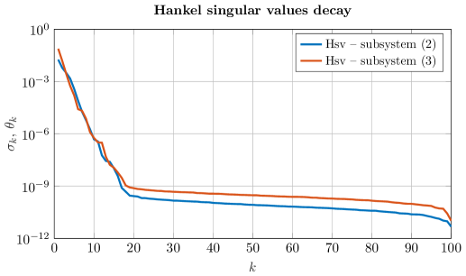
Figure 1: Decay of Hankel singular values for the subsystems (2) and (3).

For subsystem (2), we construct ROMs of orders $5$ and $10$ using balanced truncation (referred here as BT) and SPA (referred here as SPA) based on the Gramians $P_{0}$ and $Q$. Similarly, for subsystem (3), we construct ROMs of order $5$ and $10$ using balanced truncation (referred here as BT_2) and SPA (referred here as SPA_2) based on the Gramians $P_{B}$ and $Q$. In order to compare the quality of ROMs, we simulate the original system and the reduced models using the input $u(t)=e^{-t}\cos(0.5t)$, $t\in[0,1]$. In Figure 2, the pointwise absolute errors for BT and SPA are depicted in semi-log scale, i.e., the function $\epsilon(t)=|y(t)-\tilde{y}(t)|$ is computed, where $y$ and $\tilde{y}$ are, receptively, the original and reduced outputs. One can observe that the results improve once the reduced order is increased. Both methodologies produce ROMs with a similar accuracy. Similarly, in Figure 3 the pointwise absolute error plots for BT_2 and SPA_2 are presented in semi-log scale. We notice that, for this example, SPA_2 produces ROMs with a higher accuracy than BT_2. Additionally, in Tables 1 and 2, the $L^{2}$-error values for the time interval $[0,1]$ together with the corresponding error bounds for the different methods are shown, respectively, for subsystems (2) and (3).

Method	Err. bound $r_{x_{0}}=5$	$L^{2}$-err. $r_{x_{0}}=5$	Err. bound $r_{x_{0}}=10$	$L^{2}$-err. $r_{x_{0}}=10$
BT	$7.64\cdot 10^{-5}$	$2.80\cdot 10^{-5}$	$1.32\cdot 10^{-6}$	$6.76\cdot 10^{-7}$
SPA	$1.53\cdot 10^{-4}$	$5.33\cdot 10^{-5}$	$2.57\cdot 10^{-6}$	$1.77\cdot 10^{-6}$

Table 1: $L^{2}$-errors for subsystem (2): Error bounds in Theorem 4.3 and real errors for BT and SPA for the simulation presented in Figure 2.

Method	Err. bound $r_{B}=5$	$L^{2}$-err. $r_{B}=5$	Err. bound $r_{B}=10$	$L^{2}$-err. $r_{B}=10$
BT_2	$1.69\cdot 10^{-4}$	$3.25\cdot 10^{-5}$	$7.88\cdot 10^{-7}$	$5.31\cdot 10^{-8}$
SPA_2	$1.69\cdot 10^{-4}$	$3.42\cdot 10^{-6}$	$7.88\cdot 10^{-7}$	$4.00\cdot 10^{-9}$

Table 2: $L^{2}$-errors for subsystem (3): Error bound in Theorem 4.4 and real errors for BT_2 and SPA_2 for the simulation presented in Figure 3.

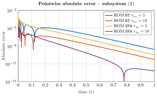
Figure 2: The pointwise absolute error for the approximations of subsystem (2) with input $u(t)=e^{-t}\cos(0.5t)$.

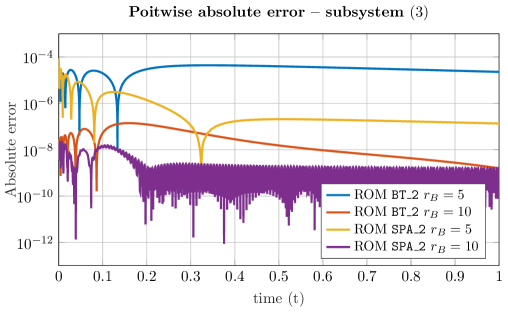
Figure 3: The pointwise absolute error for the approximations of subsystem (3) with input $u(t)=e^{-t}\cos(0.5t)$.

In Figure 4, we depict the decay of normalized $L^{2}$-error bounds from Theorem 4.3 together with the real $L^{2}$-errors produced by the time domain simulations for the subsystem (2) using the methods BT and SPA. Normalized here means to be divided by the $L^{2}$-norm of the original system output, e.g., the normalized $L^{2}$-error for a given order is $\|y-\tilde{y}\|_{L^{2}}/\|y\|_{L^{2}}$, where $\tilde{y}$ is the reduced output. For this example, BT is performing slightly better than SPA. Similarly, in Figure 5 we depict the decay of the normalized $L^{2}$-error bound from Theorem 4.4 together with the normalized $L^{2}$-errors produced by the time domain simulations for the subsystem (3) using the methods BT_2 and SPA_2. As stated before, SPA_2 produces ROMs that are more accurate than BT_2.

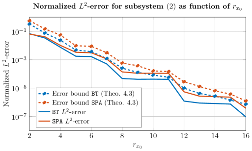
Figure 4: Subsystem (2): Decay of normalized error bound ($\text{Err. Bound}/\|y_{x_{0}}\|_{L^{2}}$) and normalized $L^{2}$-error ($\|y_{x_{0}}-\tilde{y}_{x_{0}}\|_{L^{2}}/\|y_{x_{0}}\|_{L^{2}}$) produced by SPA and BT for different orders $r_{x_{0}}=1,\dots,16$.

.

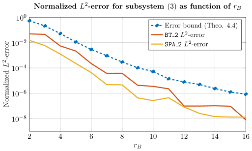
Figure 5: Subsystem (3): Decay of the normalized error bound ($\text{Err. Bound}/\|y_{B}\|_{L^{2}}$) and normalized $L^{2}$-error ($\|y_{B}-\tilde{y}_{B}\|_{L^{2}}/\|y_{B}\|_{L^{2}}$) produced by SPA_2 and BT_2 for different orders $r_{B}=1,\dots,16$.

.

Finally, we illustrate the statement of Remark 5 and show the influence of the parameter $\gamma$ on the approximation performance by means of Figure 6. This figure depicts the error bound from Theorem 4.3 and the real $L^{2}$-error as a function of $\gamma$ (see Equations (12) and (16)) for a reduced dimension $r_{x_{0}}=10$. Furthermore, the simulations are conducted using the input $u(t)=e^{-t}\cos(0.5t)$ on the interval $[0,1]$. We see that different values of $\gamma$ can lead to different qualities of the reduced models. Moreover, we observe numerically that for larger values $\gamma$, in this example $\gamma>6$, the real $L^{2}$- error is increasing again. The choice of the optimal $\gamma$ is still an open problem, but not considered in this work. The numerical example suggests that one possible strategy is to select the $\gamma$ that minimizes the error bound of Theorem 4.3.

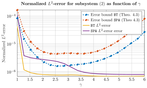
Figure 6: Subsystem (2): Normalized error bound ($\text{Err. Bound}/\|y_{x_{0}}\|_{L^{2}}$) and normalized $L^{2}$-error ($\|y_{x_{0}}-\tilde{y}_{x_{0}}\|_{L^{2}}/\|y_{x_{0}}\|_{L^{2}}$) produced by SPA and BT for different values $\gamma\in[1,6]$ and reduced dimension $r_{x_{0}}=10$.

.

Appendix A Proofs of Section 2

A.1 Proof of Lemma 2.3

Proof of Lemma 2.3.

We factorize $K=FF^{\top}$. Let $f_{i}$ be the $i$th column of the matrix $F$ and $x_{f_{i}}(\cdot,s)$ denote the solution to (2a) with initial state $f_{i}$ and initial time $s$. Then, we have

$$\Phi(t,s)F=[x_{f_{1}}(t,s),x_{f_{2}}(t,s),\ldots,x_{f_{d}}(t,s)],$$

where $d$ is the number of columns of $F$. Using the scaling $\gamma>0$, $x_{f_{i}}(\cdot,s)$ can be interpreted as the solution to $\dot{x}_{f_{i}}(t)=Ax_{f_{i}}(t)+\sum_{k=1}^{m}\frac{1}{\gamma}N_{k}x_{f_{i}}(t)\gamma u_{k}(t)$. Applying the results of (Redmann, 2021, Section 2) on a bound for $x_{f_{i}}(t,s)x_{f_{i}}^{\top}(t,s)$, we obtain

$$\Phi(t,s)K\Phi^{\top}(t,s) =\sum_{k=1}^{m}x_{f_{i}}(t,s)x_{f_{i}}^{\top}(t,s)\leq\exp\left\{\int_{s}^{t}\left\|\gamma u^{0}(v)\right\|_{2}^{2}dv\right\}\sum_{k=1}^{m}Z_{\gamma}(t-s,f_{i}f_{i}^{\top})$$

$$=\exp\left\{\int_{s}^{t}\left\|\gamma u^{0}(v)\right\|_{2}^{2}dv\right\}Z_{\gamma}(t-s,K),$$

where the second argument in $Z_{\gamma}$ denotes the respective initial condition. This concludes the proof. ∎

A.2 Proof of Theorem 2.4

Before we begin with the proof, we want to emphasize that it heavily makes use of relations between the bilinear equation (1a) and the stochastic system that results from setting $u_{k}=\frac{dw_{k}}{dt}$ in the bilinear term, where $\frac{dw_{k}}{dt}$ is white noise. Exploiting this link spares us from conducting relatively long and technical proofs. In particular, the stability analysis of bilinear and stochastic system is based on the same type of Lyapunov equations (Damm, 2004; Redmann, 2018). Therefore, the first part of the Theorem 2.4 follows from the result in (Benner ., 2016). Moreover, the state of a bilinear system can be bounded by the state of the associated stochastic differential equation (Redmann, 2021). This allows to transfer the result of (Redmann  Pontes Duff, 2022), where the existence of a matrix $V$ as in Theorem 2.4 was proved for stochastic systems. It turns out that the same holds true in the bilinear case using the same $V$ as in (Redmann  Pontes Duff, 2022).

Proof of Theorem 2.4.

Condition (8) implies (9) by (Benner ., 2016, Corollary 3.2) or (Redmann, 2016, Lemma 6.12). Now, we can use a stochastic representation for $Z_{\gamma}(\cdot,X_{0}X_{0}^{\top})$, see, e.g., (Damm, 2004; Redmann, 2018) which is $Z_{\gamma}(t,X_{0}X_{0}^{\top})=\mathbb{E}\left[\Phi_{w}(t)X_{0}X_{0}^{\top}\Phi_{w}^{\top}(t)\right]$. Here, the stochastic fundamental solution $\Phi_{w}$ satisfies $\Phi_{w}(t)=I+\int_{0}^{t}A\Phi_{w}(s)ds+\sum_{k=1}^{m}\int_{0}^{t}N_{k}\Phi_{w}(s)dw_{k}(s)$ by definition, where $w_{1},\ldots,w_{m}$ are independent standard Brownian motions. Based on (Redmann  Pontes Duff, 2022, Theorem 4.4, Remark 1), we then find

$$\left\|Z_{\gamma}(t,X_{0}X_{0}^{\top})\right\|_{2}\leq\mathbb{E}\left\|\Phi_{w}(t)X_{0}X_{0}^{\top}\Phi_{w}^{\top}(t)\right\|_{2}\leq\mathbb{E}\left\|\Phi_{w}(t)X_{0}\right\|_{F}^{2}\lesssim\operatorname{e}^{-ct}.$$

Let us finally consider

$$\left\|\Phi(t)X_{0}-V\tilde{\Phi}(t)\tilde{X}_{0}\right\|_{F}^{2} =\left\|\left[\begin{smallmatrix}{I}&-V\end{smallmatrix}\right]\left[\begin{smallmatrix}{\Phi}(t)&0\\ 0&\tilde{\Phi}(t)\end{smallmatrix}\right]\left[\begin{smallmatrix}{X}_{0}\\ \tilde{X}_{0}\end{smallmatrix}\right]\right\|_{F}^{2}$$

$$=\operatorname{tr}\left(\left[\begin{smallmatrix}{I}&-V\end{smallmatrix}\right]\left[\begin{smallmatrix}{\Phi}(t)&0\\ 0&\tilde{\Phi}(t)\end{smallmatrix}\right]\left[\begin{smallmatrix}{X}_{0}\\ \tilde{X}_{0}\end{smallmatrix}\right]\left[\begin{smallmatrix}{X}_{0}^{\top}&\tilde{X}_{0}^{\top}\end{smallmatrix}\right]\left[\begin{smallmatrix}{\Phi}^{\top}(t)&0\\ 0&\tilde{\Phi}^{\top}(t)\end{smallmatrix}\right]\left[\begin{smallmatrix}{I}\\ -V^{\top}\end{smallmatrix}\right]\right).$$

Since $\left[\begin{smallmatrix}{\Phi}(t)&0\\ 0&\tilde{\Phi}(t)\end{smallmatrix}\right]$ is the fundamental solution to a bilinear system with matrices $\left[\begin{smallmatrix}{A}&0\\ 0&\tilde{A}\end{smallmatrix}\right]$ and $\left[\begin{smallmatrix}{N}_{k}&0\\ 0&\tilde{N}_{k}\end{smallmatrix}\right]$, we can apply Lemma 2.3 leading to

$$\left\|\Phi(t)X_{0}-V\tilde{\Phi}(t)\tilde{X}_{0}\right\|_{F}^{2}\leq\operatorname{tr}\left(\left[\begin{smallmatrix}{I}&-V\end{smallmatrix}\right]Z_{\gamma}^{e}(t)\left[\begin{smallmatrix}{I}\\ -V^{\top}\end{smallmatrix}\right]\right)\exp\left\{\int_{0}^{t}\left\|\gamma u^{0}(s)\right\|_{2}^{2}ds\right\},$$

where $Z_{\gamma}^{e}$ is the matrix function solving (6) with coefficients $\left[\begin{smallmatrix}{A}&0\\ 0&\tilde{A}\end{smallmatrix}\right]$, $\left[\begin{smallmatrix}{N}_{k}&0\\ 0&\tilde{N}_{k}\end{smallmatrix}\right]$ and $K=\left[\begin{smallmatrix}{X}_{0}\\ \tilde{X}_{0}\end{smallmatrix}\right]\left[\begin{smallmatrix}{X}_{0}^{\top}&\tilde{X}_{0}^{\top}\end{smallmatrix}\right]$. We exploit the associated stochastic representation which is $Z^{e}(t)=\mathbb{E}\left(\left[\begin{smallmatrix}{\Phi}_{w}(t)&0\\ 0&\tilde{\Phi}_{w}(t)\end{smallmatrix}\right]\left[\begin{smallmatrix}{X}_{0}\\ \tilde{X}_{0}\end{smallmatrix}\right]\left[\begin{smallmatrix}{X}_{0}^{\top}&\tilde{X}_{0}^{\top}\end{smallmatrix}\right]\left[\begin{smallmatrix}{\Phi}^{\top}_{w}(t)&0\\ 0&\tilde{\Phi}^{\top}_{w}(t)\end{smallmatrix}\right]\right)$, where $\tilde{\Phi}_{w}$ is the reduced order stochastic fundamental solution involving the matrices $\tilde{A}$ and $\tilde{N}_{k}$. Consequently, based on the linearity of the trace and the definition of the Frobenius norm, we have

$$\left\|\Phi(t)X_{0}-V\tilde{\Phi}(t)\tilde{X}_{0}\right\|_{F}^{2}\leq\mathbb{E}\left\|\Phi_{w}(t)X_{0}-V\tilde{\Phi}_{w}(t)\tilde{X}_{0}\right\|_{F}^{2}\exp\left\{\int_{0}^{t}\left\|\gamma u^{0}(s)\right\|_{2}^{2}ds\right\}.$$

Due to (Redmann  Pontes Duff, 2022, Corollary 4.5, Remark 1) we know about the existence of $V$ with $V^{\top}V=I$ such that $\Phi_{w}(t)X_{0}=V\tilde{\Phi}_{w}(t)\tilde{X}_{0}$, where $\tilde{\Phi}_{w}$ decays exponentially in the mean square sense. This decay of $\tilde{\Phi}_{w}$ is equivalent to (10), see, e.g., (Damm, 2004) which concludes the proof. ∎

Appendix B Proofs of Section 4.2

B.1 Proof of Theorem 4.1

Proof of Theorem 4.1.

Since the Gramians of a balanced system are identical and equal to the diagonal matrix $\Theta$, we have

$$\left[\begin{smallmatrix}{\mathcal{A}}_{11}&{\mathcal{A}}_{12}\\ {\mathcal{A}}_{21}&{\mathcal{A}}_{22}\end{smallmatrix}\right]\left[\begin{smallmatrix}{\Theta}_{1}&\\ &{\Theta}_{2}\end{smallmatrix}\right]+\left[\begin{smallmatrix}{\Theta}_{1}&\\ &{\Theta}_{2}\end{smallmatrix}\right]\left[\begin{smallmatrix}{\mathcal{A}}_{11}^{\top}&{\mathcal{A}}_{21}^{\top}\\ {\mathcal{A}}_{12}^{\top}&{\mathcal{A}}_{22}^{\top}\end{smallmatrix}\right]+\frac{1}{\gamma^{2}}\sum_{k=1}^{m}\left[\begin{smallmatrix}{\mathcal{N}}_{k,11}&{\mathcal{N}}_{k,12}\\ {\mathcal{N}}_{k,21}&{\mathcal{N}}_{k,22}\end{smallmatrix}\right]\left[\begin{smallmatrix}{\Theta}_{1}&\\ &{\Theta}_{2}\end{smallmatrix}\right]\left[\begin{smallmatrix}{\mathcal{N}}_{k,11}^{\top}&{\mathcal{N}}_{k,21}^{\top}\\ {\mathcal{N}}_{k,12}^{\top}&{\mathcal{N}}_{k,22}^{\top}\end{smallmatrix}\right]$$

$$=-\left[\begin{smallmatrix}{X}_{0,1}\\ X_{0,2}\end{smallmatrix}\right]\left[\begin{smallmatrix}{X}_{0,1}^{\top}&X_{0,2}^{\top}\end{smallmatrix}\right],$$ (36)

$$\left[\begin{smallmatrix}{\mathcal{A}}_{11}^{\top}&{\mathcal{A}}_{21}^{\top}\\ {\mathcal{A}}_{12}^{\top}&{\mathcal{A}}_{22}^{\top}\end{smallmatrix}\right]\left[\begin{smallmatrix}{\Theta}_{1}&\\ &{\Theta}_{2}\end{smallmatrix}\right]+\left[\begin{smallmatrix}{\Theta}_{1}&\\ &{\Theta}_{2}\end{smallmatrix}\right]\left[\begin{smallmatrix}{\mathcal{A}}_{11}&{\mathcal{A}}_{12}\\ {\mathcal{A}}_{21}&{\mathcal{A}}_{22}\end{smallmatrix}\right]+\frac{1}{\gamma^{2}}\sum_{k=1}^{m}\left[\begin{smallmatrix}{\mathcal{N}}_{k,11}^{\top}&{\mathcal{N}}_{k,21}^{\top}\\ {\mathcal{N}}_{k,12}^{\top}&{\mathcal{N}}_{k,22}^{\top}\end{smallmatrix}\right]\left[\begin{smallmatrix}{\Theta}_{1}&\\ &{\Theta}_{2}\end{smallmatrix}\right]\left[\begin{smallmatrix}{\mathcal{N}}_{k,11}&{\mathcal{N}}_{k,12}\\ {\mathcal{N}}_{k,21}&{\mathcal{N}}_{k,22}\end{smallmatrix}\right]$$

$$=-\left[\begin{smallmatrix}{\mathcal{C}}_{1}^{\top}\\ {\mathcal{C}}_{2}^{\top}\end{smallmatrix}\right]\left[\begin{smallmatrix}{\mathcal{C}}_{1}&{\mathcal{C}}_{2}\end{smallmatrix}\right].$$ (37)

The left upper blocks of these equations yield

$${\mathcal{A}}_{11}\Theta_{1}+\Theta_{1}{\mathcal{A}}_{11}^{\top}+\frac{1}{\gamma^{2}}\sum_{k=1}^{m}{\mathcal{N}}_{k,11}\Theta_{1}{\mathcal{N}}_{k,11}^{\top} \leq-X_{0,1}X_{0,1}^{\top},$$ (38)

$${\mathcal{A}}_{11}^{\top}\Theta_{1}+\Theta_{1}{\mathcal{A}}_{11}+\frac{1}{\gamma^{2}}\sum_{k=1}^{m}{\mathcal{N}}_{k,11}^{\top}\Theta_{1}{\mathcal{N}}_{k,11} \leq-{\mathcal{C}}_{1}^{\top}{\mathcal{C}}_{1}.$$

Therefore, $\tilde{Z}_{\gamma}$ and $\tilde{Z}_{\gamma}^{*}$ decay exponentially by Theorem 2.4 if BT is considered. Consequently, the integrals $\tilde{P}$ and $\tilde{Q}$ exist. We now multiply (37) by

$$\begin{bmatrix}{\mathcal{A}}_{11}&{\mathcal{A}}_{12}\\ {\mathcal{A}}_{21}&{\mathcal{A}}_{22}\end{bmatrix}^{-1}=\begin{bmatrix}\bar{\mathcal{A}}^{-1}&\star\ {}\\ -{\mathcal{A}}_{22}^{-1}{\mathcal{A}}_{21}\bar{\mathcal{A}}^{-1}&\star\ {}\end{bmatrix}$$ (39)

from the right and with its transposed from the left. Evaluating the left upper block of the resulting equation and multiplying it with $\bar{\mathcal{A}}$ from the right and its transposed from the left, we find

$$\bar{\mathcal{A}}^{\top}\Theta_{1}+\Theta_{1}\bar{\mathcal{A}}+\frac{1}{\gamma^{2}}\sum_{k=1}^{m}\bar{\mathcal{N}}_{k}^{\top}\Theta_{1}\bar{\mathcal{N}}_{k}=-\bar{\mathcal{C}}^{\top}\bar{\mathcal{C}}-\frac{1}{\gamma^{2}}\sum_{k=1}^{m}\bar{\mathcal{N}}_{k,21}^{\top}\Theta_{2}\bar{\mathcal{N}}_{k,21}\leq-\bar{\mathcal{C}}^{\top}\bar{\mathcal{C}},$$ (40)

where $\bar{\mathcal{N}}_{k,21}:={\mathcal{N}}_{k,21}-{\mathcal{N}}_{k,22}{\mathcal{A}}_{22}^{-1}{\mathcal{A}}_{21}$ providing the existence of $\tilde{Q}$ for SPA using Theorem 2.4. ∎

B.2 Proof of Lemma 4.2

Proof of Lemma 4.2.

By Lemma 2.2, we have that $y_{x_{0}}(t)=C\Phi(t)X_{0}v_{0}$ and $y_{x_{0}}(t)=\tilde{C}_{x_{0}}\tilde{\Phi}(t)\tilde{X}_{0}v_{0}$, where $\Phi$ and $\tilde{\Phi}$ are the fundamental solutions to the original and the reduced system, respectively, introduced in Definition 2.1. Consequently, we obtain

$$\left\|y_{x_{0}}(t)-\tilde{y}_{x_{0}}(t)\right\|_{2}^{2} \leq\left\|C\Phi(t)X_{0}-\tilde{C}_{x_{0}}\tilde{\Phi}(t)\tilde{X}_{0}\right\|_{F}^{2}\left\|v_{0}\right\|_{2}^{2}=\left\|\left[\begin{smallmatrix}{C}&-\tilde{C}_{x_{0}}\end{smallmatrix}\right]\left[\begin{smallmatrix}{\Phi}(t)&0\\ 0&\tilde{\Phi}(t)\end{smallmatrix}\right]\left[\begin{smallmatrix}{X}_{0}\\ \tilde{X}_{0}\end{smallmatrix}\right]\right\|_{F}^{2}\left\|v_{0}\right\|_{2}^{2}$$

$$=\operatorname{tr}\left(\left[\begin{smallmatrix}{C}&-\tilde{C}_{x_{0}}\end{smallmatrix}\right]\left[\begin{smallmatrix}{\Phi}(t)&0\\ 0&\tilde{\Phi}(t)\end{smallmatrix}\right]\left[\begin{smallmatrix}{X}_{0}\\ \tilde{X}_{0}\end{smallmatrix}\right]\left[\begin{smallmatrix}{X}_{0}^{\top}&\tilde{X}_{0}^{\top}\end{smallmatrix}\right]\left[\begin{smallmatrix}{\Phi}^{\top}(t)&0\\ 0&\tilde{\Phi}^{\top}(t)\end{smallmatrix}\right]\left[\begin{smallmatrix}{C}^{\top}\\ -C_{x_{0}}^{\top}\end{smallmatrix}\right]\right)\left\|v_{0}\right\|_{2}^{2}.$$

Now, $\left[\begin{smallmatrix}{\Phi}(t)&0\\ 0&\tilde{\Phi}(t)\end{smallmatrix}\right]$ is the fundamental solution to the bilinear system with matrices $\left[\begin{smallmatrix}{A}&0\\ 0&\tilde{A}_{x_{0}}\end{smallmatrix}\right]$ and $\left[\begin{smallmatrix}{N}_{k}&0\\ 0&\tilde{N}_{x_{0},k}\end{smallmatrix}\right]$. Therefore, the result follows by Lemma 2.3 setting $K=\left[\begin{smallmatrix}{X}_{0}\\ \tilde{X}_{0}\end{smallmatrix}\right]\left[\begin{smallmatrix}{X}_{0}^{\top}&\tilde{X}_{0}^{\top}\end{smallmatrix}\right]$. ∎

B.3 Proof of Theorem 4.3

Proof of Theorem 4.3.

We integrate the result of Lemma 4.2 on $[0,\infty)$ and obtain

$$\left\|y_{x_{0}}-\tilde{y}_{x_{0}}\right\|_{L^{2}}^{2}\leq\mathcal{E}\exp\left\{\left\|\gamma u^{0}\right\|_{L^{2}}^{2}\right\}\left\|v_{0}\right\|_{2}^{2},$$

where $\mathcal{E}:=\operatorname{tr}\left(\left[\begin{smallmatrix}{C}&-\tilde{C}_{x_{0}}\end{smallmatrix}\right]\int_{0}^{\infty}Z_{\gamma}^{e}(t)dt\left[\begin{smallmatrix}{C}^{\top}\\ -\tilde{C}_{x_{0}}^{\top}\end{smallmatrix}\right]\right)$. The left upper and the right lower block of $\int_{0}^{\infty}Z_{\gamma}^{e}(t)dt$ are $P_{0}$ and $\tilde{P}$, respectively. Both Gramians exist by assumption and Theorem 4.1. This also implies the existence of the right upper block of $\int_{0}^{\infty}Z_{\gamma}^{e}(t)dt$ which we denote by $\widehat{P}$. It satisfies

$$A\widehat{P}+\widehat{P}\tilde{A}_{x_{0}}^{\top}+\frac{1}{\gamma^{2}}\sum_{k=1}^{m}N_{k}\widehat{P}\tilde{N}_{x_{0},k}^{\top}=-X_{0}X_{0,1}^{\top}.$$ (41)

Let $\mathcal{S}$ be the matrix ensuring (25). Since $\Theta=\mathcal{S}P_{0}\mathcal{S}^{\top}$, $Y=\mathcal{S}\widehat{P}$ and $\left[\begin{smallmatrix}{\mathcal{C}}_{1}&{\mathcal{C}}_{2}\end{smallmatrix}\right]=C\mathcal{S}^{-1}$, we have

$$\mathcal{E}= \operatorname{tr}(CP_{0}C^{\top})+\operatorname{tr}(\tilde{C}_{x_{0}}\tilde{P}\tilde{C}_{x_{0}}^{\top})-2\operatorname{tr}(C\widehat{P}\tilde{C}_{x_{0}}^{\top})$$

$$=\operatorname{tr}(\left[\begin{smallmatrix}{\mathcal{C}}_{1}&{\mathcal{C}}_{2}\end{smallmatrix}\right]\left[\begin{smallmatrix}{\Theta}_{1}&\\ &{\Theta}_{2}\end{smallmatrix}\right]\left[\begin{smallmatrix}{\mathcal{C}}_{1}^{\top}\\ {\mathcal{C}}_{2}^{\top}\end{smallmatrix}\right])+\operatorname{tr}(\tilde{C}_{x_{0}}\tilde{P}_{0}\tilde{C}_{x_{0}}^{\top})-2\operatorname{tr}(\left[\begin{smallmatrix}{\mathcal{C}}_{1}&{\mathcal{C}}_{2}\end{smallmatrix}\right]Y\tilde{C}_{x_{0}}^{\top}).$$

Comparing (36) with (37), we see that $\operatorname{tr}(\left[\begin{smallmatrix}{\mathcal{C}}_{1}&{\mathcal{C}}_{2}\end{smallmatrix}\right]\Theta\left[\begin{smallmatrix}{\mathcal{C}}_{1}^{\top}\\ {\mathcal{C}}_{2}^{\top}\end{smallmatrix}\right])=\operatorname{tr}(\left[\begin{smallmatrix}{X}_{0,1}^{\top}&{X}_{0,2}^{\top}\end{smallmatrix}\right]\Theta\left[\begin{smallmatrix}{X}_{0,1}\\ {X}_{0,2}\end{smallmatrix}\right])$. Since the same is true for the reduced Gramians, we obtain

$$\mathcal{E}=\operatorname{tr}(\left[\begin{smallmatrix}{X}_{0,1}^{\top}&{X}_{0,2}^{\top}\end{smallmatrix}\right]\left[\begin{smallmatrix}{\Theta}_{1}&\\ &{\Theta}_{2}\end{smallmatrix}\right]\left[\begin{smallmatrix}{X}_{0,1}\\ {X}_{0,2}\end{smallmatrix}\right])+\operatorname{tr}({X}_{0,1}^{\top}\tilde{Q}{X}_{0,1})-2\operatorname{tr}(\left[\begin{smallmatrix}{\mathcal{C}}_{1}&{\mathcal{C}}_{2}\end{smallmatrix}\right]Y\tilde{C}_{x_{0}}^{\top}),$$ (42)

where $\tilde{Q}$ exists due to Theorem 4.1. Now, it is needed to find an equation for $\tilde{C}_{x_{0}}^{\top}\left[\begin{smallmatrix}{\mathcal{C}}_{1}&{\mathcal{C}}\end{smallmatrix}\right]$ for both BT and SPA in order to analyze the error further. We evaluate the first $r_{x_{0}}$ rows of (37) to obtain an expression for the case of BT:

$$-{\mathcal{C}}_{1}^{\top}\left[\begin{smallmatrix}{\mathcal{C}}_{1}&{\mathcal{C}}_{2}\end{smallmatrix}\right]=\left[\begin{smallmatrix}{\mathcal{A}}_{11}^{\top}{\Theta}_{1}&{\mathcal{A}}_{21}^{\top}{\Theta}_{2}\end{smallmatrix}\right]+\left[\begin{smallmatrix}{\Theta}_{1}&0\end{smallmatrix}\right]\left[\begin{smallmatrix}{\mathcal{A}}_{11}&{\mathcal{A}}_{12}\\ {\mathcal{A}}_{21}&{\mathcal{A}}_{22}\end{smallmatrix}\right]+\frac{1}{\gamma^{2}}\sum_{k=1}^{m}\left[\begin{smallmatrix}{\mathcal{N}}_{k,11}^{\top}{\Theta}_{1}&{\mathcal{N}}_{k,21}^{\top}{\Theta}_{2}\end{smallmatrix}\right]\left[\begin{smallmatrix}{\mathcal{N}}_{k,11}&{\mathcal{N}}_{k,12}\\ {\mathcal{N}}_{k,21}&{\mathcal{N}}_{k,22}\end{smallmatrix}\right].$$ (43)

For SPA we multiply (37) with $\left[\begin{smallmatrix}{\mathcal{A}}_{11}^{\top}&{\mathcal{A}}_{21}^{\top}\\ {\mathcal{A}}_{12}^{\top}&{\mathcal{A}}_{22}^{\top}\end{smallmatrix}\right]^{-1}$ from the left and obtain

$$-\left[\begin{smallmatrix}{\bar{\mathcal{A}}}^{-\top}{\bar{\mathcal{C}}}^{\top}\\ \star\end{smallmatrix}\right]\left[\begin{smallmatrix}{\mathcal{C}}_{1}&{\mathcal{C}}_{2}\end{smallmatrix}\right]= \left[\begin{smallmatrix}{\Theta}_{1}&\\ &{\Theta}_{2}\end{smallmatrix}\right]+\left[\begin{smallmatrix}{\bar{\mathcal{A}}}^{-\top}&-\bar{\mathcal{A}}^{-\top}({\mathcal{A}}_{22}^{-1}{\mathcal{A}}_{21})^{\top}\\ \star&\star\end{smallmatrix}\right]\left[\begin{smallmatrix}{\Theta}_{1}&\\ &{\Theta}_{2}\end{smallmatrix}\right]\left[\begin{smallmatrix}{\mathcal{A}}_{11}&{\mathcal{A}}_{12}\\ {\mathcal{A}}_{21}&{\mathcal{A}}_{22}\end{smallmatrix}\right]$$

$$+\frac{1}{\gamma^{2}}\sum_{k=1}^{m}\left[\begin{smallmatrix}{\bar{\mathcal{A}}}^{-\top}{\bar{\mathcal{N}}}_{k}^{\top}&{\bar{\mathcal{A}}}^{-\top}\bar{\mathcal{N}}_{k,21}^{\top}\\ \star&\star\end{smallmatrix}\right]\left[\begin{smallmatrix}{\Theta}_{1}&\\ &{\Theta}_{2}\end{smallmatrix}\right]\left[\begin{smallmatrix}{\mathcal{N}}_{k,11}&{\mathcal{N}}_{k,12}\\ {\mathcal{N}}_{k,21}&{\mathcal{N}}_{k,22}\end{smallmatrix}\right]$$

using the partition in (39) and setting $\bar{\mathcal{N}}_{k,21}:={\mathcal{N}}_{k,21}-{\mathcal{N}}_{k,22}{\mathcal{A}}_{22}^{-1}{\mathcal{A}}_{21}$. Multiplying the first $r_{x_{0}}$ rows of the above equation by $\bar{\mathcal{A}}^{\top}$ from the left results in

$$-\bar{\mathcal{C}}^{\top}\left[\begin{smallmatrix}{\mathcal{C}}_{1}&{\mathcal{C}}_{2}\end{smallmatrix}\right]=\bar{\mathcal{A}}^{\top}{\Theta}_{1}+\left[\begin{smallmatrix}{\Theta_{1}}&-({\mathcal{A}}_{22}^{-1}{\mathcal{A}}_{21})^{\top}\Theta_{2}\end{smallmatrix}\right]\left[\begin{smallmatrix}{\mathcal{A}}_{11}&{\mathcal{A}}_{12}\\ {\mathcal{A}}_{21}&{\mathcal{A}}_{22}\end{smallmatrix}\right]+\frac{1}{\gamma^{2}}\sum_{k=1}^{m}\left[\begin{smallmatrix}{\bar{\mathcal{N}}}_{k}^{\top}{\Theta}_{1}&{\bar{\mathcal{N}}}_{k,21}^{\top}{\Theta}_{2}\end{smallmatrix}\right]\left[\begin{smallmatrix}{\mathcal{N}}_{k,11}&{\mathcal{N}}_{k,12}\\ {\mathcal{N}}_{k,21}&{\mathcal{N}}_{k,22}\end{smallmatrix}\right].$$ (44)

We summarize (43) and (44) to one equation. That is

$$-\tilde{C}_{x_{0}}^{\top}\left[\begin{smallmatrix}{\mathcal{C}}_{1}&{\mathcal{C}}_{2}\end{smallmatrix}\right]=\left[\begin{smallmatrix}{\tilde{A}}_{x_{0}}^{\top}{\Theta}_{1}&{\mathbf{A}}_{21}^{\top}{\Theta}_{2}\end{smallmatrix}\right]+\left[\begin{smallmatrix}{\Theta_{1}}&{\bar{\mathbf{A}}}_{21}^{\top}\Theta_{2}\end{smallmatrix}\right]\left[\begin{smallmatrix}{\mathcal{A}}_{11}&{\mathcal{A}}_{12}\\ {\mathcal{A}}_{21}&{\mathcal{A}}_{22}\end{smallmatrix}\right]+\frac{1}{\gamma^{2}}\sum_{k=1}^{m}\left[\begin{smallmatrix}{\tilde{N}}_{x_{0},k}^{\top}{\Theta}_{1}&{\mathbf{N}}_{k,21}^{\top}{\Theta}_{2}\end{smallmatrix}\right]\left[\begin{smallmatrix}{\mathcal{N}}_{k,11}&{\mathcal{N}}_{k,12}\\ {\mathcal{N}}_{k,21}&{\mathcal{N}}_{k,22}\end{smallmatrix}\right].$$

where ${\mathbf{A}}_{21}\in\{\mathcal{A}_{21},0\}$, $\bar{\mathbf{A}}_{21}\in\{0,-{\mathcal{A}}_{22}^{-1}{\mathcal{A}}_{21}\}$ and ${\mathbf{N}}_{k,21}\in\{\mathcal{N}_{k,21},{\bar{\mathcal{N}}}_{k,21}\}$. Inserting this into $\operatorname{tr}(\left[\begin{smallmatrix}{\mathcal{C}}_{1}&{\mathcal{C}}_{2}\end{smallmatrix}\right]Y\tilde{C}_{x_{0}}^{\top})$ yields

$$-\operatorname{tr}(\left[\begin{smallmatrix}{\mathcal{C}}_{1}&{\mathcal{C}}_{2}\end{smallmatrix}\right]Y\tilde{C}_{x_{0}}^{\top})$$

$$=\operatorname{tr}\left(Y\left[\left[\begin{smallmatrix}{\tilde{A}}_{x_{0}}^{\top}{\Theta}_{1}&{\mathbf{A}}_{21}^{\top}{\Theta}_{2}\end{smallmatrix}\right]+\left[\begin{smallmatrix}{\Theta_{1}}&{\bar{\mathbf{A}}}_{21}^{\top}\Theta_{2}\end{smallmatrix}\right]\left[\begin{smallmatrix}{\mathcal{A}}_{11}&{\mathcal{A}}_{12}\\ {\mathcal{A}}_{21}&{\mathcal{A}}_{22}\end{smallmatrix}\right]+\frac{1}{\gamma^{2}}\sum_{k=1}^{m}\left[\begin{smallmatrix}{\tilde{N}}_{x_{0},k}^{\top}{\Theta}_{1}&{\mathbf{N}}_{k,21}^{\top}{\Theta}_{2}\end{smallmatrix}\right]\left[\begin{smallmatrix}{\mathcal{N}}_{k,11}&{\mathcal{N}}_{k,12}\\ {\mathcal{N}}_{k,21}&{\mathcal{N}}_{k,22}\end{smallmatrix}\right]\right]\right)$$

$$=\operatorname{tr}\left(\Theta_{1}\left[\left[\begin{smallmatrix}{\mathcal{A}}_{11}&{\mathcal{A}}_{12}\end{smallmatrix}\right]Y+Y_{1}{\tilde{A}}_{x_{0}}^{\top}+\frac{1}{\gamma^{2}}\sum_{k=1}^{m}\left[\begin{smallmatrix}{\mathcal{N}}_{k,11}&{\mathcal{N}}_{k,12}\end{smallmatrix}\right]Y{\tilde{N}}_{x_{0},k}^{\top}\right]\right)$$

$$\quad+\operatorname{tr}\left(\Theta_{2}\left[Y_{2}{\mathbf{A}}_{21}^{\top}+\left[\begin{smallmatrix}{\mathcal{A}}_{21}&{\mathcal{A}}_{22}\end{smallmatrix}\right]Y{\bar{\mathbf{A}}}_{21}^{\top}+\frac{1}{\gamma^{2}}\sum_{k=1}^{m}\left[\begin{smallmatrix}{\mathcal{N}}_{k,21}&{\mathcal{N}}_{k,22}\end{smallmatrix}\right]Y{\mathbf{N}}_{k,21}^{\top}\right]\right).$$

The first $r_{x_{0}}$ rows of (30) give us

$$-\operatorname{tr}(\left[\begin{smallmatrix}{\mathcal{C}}_{1}&{\mathcal{C}}_{2}\end{smallmatrix}\right]Y\mathcal{C}_{1}^{\top})= -\operatorname{tr}\left(X_{0,1}^{\top}\Theta_{1}X_{0,1}\right)$$

$$+\operatorname{tr}\left(\Theta_{2}\left[Y_{2}{\mathbf{A}}_{21}^{\top}+\left[\begin{smallmatrix}{\mathcal{A}}_{21}&{\mathcal{A}}_{22}\end{smallmatrix}\right]Y{\bar{\mathbf{A}}}_{21}^{\top}+\frac{1}{\gamma^{2}}\sum_{k=1}^{m}\left[\begin{smallmatrix}{\mathcal{N}}_{k,21}&{\mathcal{N}}_{k,22}\end{smallmatrix}\right]Y{\mathbf{N}}_{k,21}^{\top}\right]\right).$$

Inserting this into (42) leads to

$$\mathcal{E}= \operatorname{tr}(X_{0,1}^{\top}(\tilde{Q}-\Theta_{1})X_{0,1})$$

$$+\operatorname{tr}\left(\Theta_{2}\left[X_{0,2}X_{0,2}^{\top}+2Y_{2}{\mathbf{A}}_{21}^{\top}+2\left[\begin{smallmatrix}{\mathcal{A}}_{21}&{\mathcal{A}}_{22}\end{smallmatrix}\right]Y{\bar{\mathbf{A}}}_{21}^{\top}+\frac{2}{\gamma^{2}}\sum_{k=1}^{m}\left[\begin{smallmatrix}{\mathcal{N}}_{k,21}&{\mathcal{N}}_{k,22}\end{smallmatrix}\right]Y{\mathbf{N}}_{k,21}^{\top}\right]\right),$$

By the left upper $r_{x_{0}}\times r_{x_{0}}$ block of (37) (BT) and (40) (SPA), it holds that

$${\tilde{A}}_{x_{0}}^{\top}\Theta_{1}+\Theta_{1}{\tilde{A}}_{x_{0}}+\frac{1}{\gamma^{2}}\sum_{k=1}^{m}{\tilde{N}}_{x_{0},k}^{\top}\Theta_{1}{\tilde{N}}_{x_{0},k}=-{\tilde{C}}_{x_{0}}^{\top}{\tilde{C}}_{x_{0}}-\frac{1}{\gamma^{2}}\sum_{k=1}^{m}\mathbf{N}_{k,21}^{\top}\Theta_{2}\mathbf{N}_{k,21}$$

for both reduced order schemes. Subtracting this identity from the equation for the reduced Gramian $\tilde{Q}$, we find

$${\tilde{A}}_{x_{0}}^{\top}(\tilde{Q}-\Theta_{1})+(\tilde{Q}-\Theta_{1}){\tilde{A}}_{x_{0}}+\frac{1}{\gamma^{2}}\sum_{k=1}^{m}{\tilde{N}}_{x_{0},k}^{\top}(\tilde{Q}-\Theta_{1}){\tilde{N}}_{x_{0},k}=\frac{1}{\gamma^{2}}\sum_{k=1}^{m}\mathbf{N}_{k,21}^{\top}\Theta_{2}\mathbf{N}_{k,21}.$$

Hence, exploiting the equation for $\tilde{P}$, we have

$$\operatorname{tr}(X_{0,1}^{\top}(\tilde{Q}-\Theta_{1})X_{0,1})=-\operatorname{tr}\left(\left[{\tilde{A}}_{x_{0}}\tilde{P}+\tilde{P}{\tilde{A}}_{x_{0}}^{\top}+\frac{1}{\gamma^{2}}\sum_{k=1}^{m}{\tilde{N}}_{x_{0},k}\tilde{P}{\tilde{N}}_{x_{0},k}^{\top}\right](\tilde{Q}-\Theta_{1})\right)$$

$$=-\operatorname{tr}\left(\tilde{P}\left[{\tilde{A}}_{x_{0}}^{\top}(\tilde{Q}-\Theta_{1})\ +(\tilde{Q}-\Theta_{1})\ {\tilde{A}}_{x_{0}}+\frac{1}{\gamma^{2}}\sum_{k=1}^{m}{\tilde{N}}_{x_{0},k}^{\top}(\tilde{Q}-\Theta_{1})\ {\tilde{N}}_{x_{0},k}\right]\right)$$

$$=-\operatorname{tr}\left(\Theta_{2}\frac{1}{\gamma^{2}}\sum_{k=1}^{m}\mathbf{N}_{k,21}\tilde{P}\mathbf{N}_{k,21}^{\top}\right),$$

which concludes the proof of this theorem. ∎

References

- Al-Baiyat \BBA Bettayeb (\APACyear1993) \APACinsertmetastartypeIBT{APACrefauthors}Al-Baiyat, S\BPBIA.\BCBT \BBA Bettayeb, M. \APACrefYearMonthDay1993. \BBOQ\APACrefatitleA new model reduction scheme for k–power bilinear systems A new model reduction scheme for k–power bilinear systems.\BBCQ \APACjournalVolNumPagesProceedings of the 32nd IEEE Conference on Decision and Control22–27. \PrintBackRefs\CurrentBib
- Antoulas \BOthers. (\APACyear2016) \APACinsertmetastarloewener_bil{APACrefauthors}Antoulas, A\BPBIC., Gosea, I\BPBIV.\BCBL \BBA Ionita, A\BPBIC. \APACrefYearMonthDay2016. \BBOQ\APACrefatitleModel Reduction of Bilinear Systems in the Loewner Framework Model Reduction of Bilinear Systems in the Loewner Framework.\BBCQ \APACjournalVolNumPagesSIAM J. Sci. Comput.385B889–B916. \PrintBackRefs\CurrentBib
- Bauer \BOthers. (\APACyear2014) \APACinsertmetastarBauerBenner_inhom{APACrefauthors}Bauer, U., Benner, P.\BCBL \BBA Feng, L. \APACrefYearMonthDay2014. \BBOQ\APACrefatitleModel Order Reduction for Linear and Nonlinear Systems: A System-Theoretic Perspective Model Order Reduction for Linear and Nonlinear Systems: A System-Theoretic Perspective.\BBCQ \APACjournalVolNumPagesArch. Comput. Methods Eng.214331–358. \PrintBackRefs\CurrentBib
- Beattie \BOthers. (\APACyear2017) \APACinsertmetastarinhom_lin{APACrefauthors}Beattie, C., Gugercin, S.\BCBL \BBA Mehrmann, V. \APACrefYearMonthDay2017. \BBOQ\APACrefatitleModel reduction for systems with inhomogeneous initial conditions Model reduction for systems with inhomogeneous initial conditions.\BBCQ \APACjournalVolNumPagesSyst. Control. Lett.9999–106. \PrintBackRefs\CurrentBib
- Benner \BBA Breiten (\APACyear2012) \APACinsertmetastarbreiten_benner{APACrefauthors}Benner, P.\BCBT \BBA Breiten, T. \APACrefYearMonthDay2012. \BBOQ\APACrefatitleInterpolation-based -model reduction of bilinear control systems Interpolation-based -model reduction of bilinear control systems.\BBCQ \APACjournalVolNumPagesSIAM J. Matrix Anal. Appl.333859–885. \PrintBackRefs\CurrentBib
- Benner \BBA Damm (\APACyear2011) \APACinsertmetastarbennerdamm{APACrefauthors}Benner, P.\BCBT \BBA Damm, T. \APACrefYearMonthDay2011. \BBOQ\APACrefatitleLyapunov equations, energy functionals, and model order reduction of bilinear and stochastic systems. Lyapunov equations, energy functionals, and model order reduction of bilinear and stochastic systems.\BBCQ \APACjournalVolNumPagesSIAM J. Control Optim.492686–711. {APACrefDOI} \doi10.1137/09075041X \PrintBackRefs\CurrentBib
- Benner \BOthers. (\APACyear2016) \APACinsertmetastarredbendamm{APACrefauthors}Benner, P., Damm, T., Redmann, M.\BCBL \BBA Rodriguez Cruz, Y\BPBIR. \APACrefYearMonthDay2016. \BBOQ\APACrefatitlePositive Operators and Stable Truncation Positive Operators and Stable Truncation.\BBCQ \APACjournalVolNumPagesLinear Algebra Appl49874–87. \PrintBackRefs\CurrentBib
- Benner \BOthers. (\APACyear2017) \APACinsertmetastarbennerdammcruz{APACrefauthors}Benner, P., Damm, T.\BCBL \BBA Rodriguez Cruz, Y\BPBIR. \APACrefYearMonthDay2017. \BBOQ\APACrefatitleDual pairs of generalized Lyapunov inequalities and balanced truncation of stochastic linear systems Dual pairs of generalized Lyapunov inequalities and balanced truncation of stochastic linear systems.\BBCQ \APACjournalVolNumPagesIEEE Trans. Autom. Contr.622782–791. \PrintBackRefs\CurrentBib
- Cao \BOthers. (\APACyear2020) \APACinsertmetastarinhom_bil{APACrefauthors}Cao, X., Benner, P., Pontes Duff, I.\BCBL \BBA Schilders, W. \APACrefYearMonthDay2020. \BBOQ\APACrefatitleModel order reduction for bilinear control systems with inhomogeneous initial conditions Model order reduction for bilinear control systems with inhomogeneous initial conditions.\BBCQ \APACjournalVolNumPagesInt. J. Control. \PrintBackRefs\CurrentBib
- Damm (\APACyear2004) \APACinsertmetastardamm{APACrefauthors}Damm, T. \APACrefYear2004. \APACrefbtitleRational Matrix Equations in Stochastic Control. Rational Matrix Equations in Stochastic Control. \APACaddressPublisherLecture Notes in Control and Information Sciences 297. Berlin: Springer. \PrintBackRefs\CurrentBib
- Damm \BBA Benner (\APACyear2014) \APACinsertmetastardammbennernewansatz{APACrefauthors}Damm, T.\BCBT \BBA Benner, P. \APACrefYearMonthDay2014. \BBOQ\APACrefatitleBalanced truncation for stochastic linear systems with guaranteed error bound Balanced truncation for stochastic linear systems with guaranteed error bound.\BBCQ \APACjournalVolNumPagesProceedings of MTNS–2014, Groningen, The Netherlands1492–1497. \PrintBackRefs\CurrentBib
- Daragmeh \BOthers. (\APACyear2019) \APACinsertmetastarspa_inhom{APACrefauthors}Daragmeh, A., Hartmann, C.\BCBL \BBA Qatanani, N. \APACrefYearMonthDay2019. \BBOQ\APACrefatitleBalanced model reduction of linear systems with nonzero initial conditions: Singular perturbation approximation Balanced model reduction of linear systems with nonzero initial conditions: Singular perturbation approximation.\BBCQ \APACjournalVolNumPagesAppl. Math. Comput.353295–307. \PrintBackRefs\CurrentBib
- D’Alessandro \BOthers. (\APACyear1974) \APACinsertmetastard1974realization{APACrefauthors}D’Alessandro, P., Isidori, A.\BCBL \BBA Ruberti, A. \APACrefYearMonthDay1974. \BBOQ\APACrefatitleRealization and structure theory of bilinear dynamical systems Realization and structure theory of bilinear dynamical systems.\BBCQ \APACjournalVolNumPagesSIAM Journal on Control123517–535. \PrintBackRefs\CurrentBib
- Flagg \BBA Gugercin (\APACyear2015) \APACinsertmetastarflagggug{APACrefauthors}Flagg, G.\BCBT \BBA Gugercin, S. \APACrefYearMonthDay2015. \BBOQ\APACrefatitleMultipoint Volterra Series Interpolation and Optimal Model Reduction of Bilinear Systems Multipoint Volterra Series Interpolation and Optimal Model Reduction of Bilinear Systems.\BBCQ \APACjournalVolNumPagesSIAM J. Matrix Anal. Appl362549–579. \PrintBackRefs\CurrentBib
- Hartmann \BOthers. (\APACyear2013) \APACinsertmetastarhartmann{APACrefauthors}Hartmann, C., Schäfer-Bung, B.\BCBL \BBA Thöns-Zueva, A. \APACrefYearMonthDay2013. \BBOQ\APACrefatitleBalanced averaging of bilinear systems with applications to stochastic control. Balanced averaging of bilinear systems with applications to stochastic control.\BBCQ \APACjournalVolNumPagesSIAM J. Control Optim.5132356–2378. {APACrefDOI} \doi10.1137/100796844 \PrintBackRefs\CurrentBib
- Heinkenschloss \BOthers. (\APACyear2011) \APACinsertmetastarHeinReisAn{APACrefauthors}Heinkenschloss, M., Reis, T.\BCBL \BBA Antoulas, A\BPBIC. \APACrefYearMonthDay2011. \BBOQ\APACrefatitleBalanced truncation model reduction for systems with inhomogeneous initial conditions Balanced truncation model reduction for systems with inhomogeneous initial conditions.\BBCQ \APACjournalVolNumPagesAutomatica473559–564. \PrintBackRefs\CurrentBib
- Huang \BOthers. (\APACyear2021) \APACinsertmetastarhuang2021splitting{APACrefauthors}Huang, Y., Jiang, Y\BHBIL.\BCBL \BBA Qiu, Z\BHBIY. \APACrefYearMonthDay2021. \BBOQ\APACrefatitleSplitting model reduction for bilinear control systems Splitting model reduction for bilinear control systems.\BBCQ \APACjournalVolNumPagesAsian Journal of Control. \PrintBackRefs\CurrentBib
- Lofberg (\APACyear2004) \APACinsertmetastarlofberg2004yalmip{APACrefauthors}Lofberg, J. \APACrefYearMonthDay2004. \BBOQ\APACrefatitleYALMIP: A toolbox for modeling and optimization in MATLAB YALMIP: A toolbox for modeling and optimization in MATLAB.\BBCQ \BIn \APACrefbtitle2004 IEEE international conference on robotics and automation (IEEE Cat. No. 04CH37508) 2004 ieee international conference on robotics and automation (ieee cat. no. 04ch37508) (\BPGS 284–289). \PrintBackRefs\CurrentBib
- Redmann (\APACyear2016) \APACinsertmetastarredmannPhD{APACrefauthors}Redmann, M. \APACrefYear2016. \APACrefbtitleModel Order Reduction Techniques Applied to Evolution Equations with Lévy Noise Model Order Reduction Techniques Applied to Evolution Equations with Lévy Noise \APACtypeAddressSchool\BUPhD. \APACaddressSchoolOtto-von-Guericke-Universität Magdeburg. \PrintBackRefs\CurrentBib
- Redmann (\APACyear2018) \APACinsertmetastarredmannspa2{APACrefauthors}Redmann, M. \APACrefYearMonthDay2018. \BBOQ\APACrefatitleType II singular perturbation approximation for linear systems with Lévy noise Type II singular perturbation approximation for linear systems with Lévy noise.\BBCQ \APACjournalVolNumPagesSIAM J. Control Optim.5632120–2158. \PrintBackRefs\CurrentBib
- Redmann (\APACyear2020\APACexlab\BCnt1) \APACinsertmetastarredstochbil{APACrefauthors}Redmann, M. \APACrefYearMonthDay2020\BCnt1. \BBOQ\APACrefatitleEnergy estimates and model order reduction for stochastic bilinear systems Energy estimates and model order reduction for stochastic bilinear systems.\BBCQ \APACjournalVolNumPagesInt. J. Control9381954–1963. \PrintBackRefs\CurrentBib
- Redmann (\APACyear2020\APACexlab\BCnt2) \APACinsertmetastarredmannstochbilspa{APACrefauthors}Redmann, M. \APACrefYearMonthDay2020\BCnt2. \BBOQ\APACrefatitleA new type of singular perturbation approximation for stochastic bilinear systems A new type of singular perturbation approximation for stochastic bilinear systems.\BBCQ \APACjournalVolNumPagesMath. Control. Signals, Syst.32129–156. \PrintBackRefs\CurrentBib
- Redmann (\APACyear2021) \APACinsertmetastarh2_bil{APACrefauthors}Redmann, M. \APACrefYearMonthDay2021. \BBOQ\APACrefatitleBilinear systems – A new link to -norms, relations to stochastic systems and further properties Bilinear systems – A new link to -norms, relations to stochastic systems and further properties.\BBCQ \APACjournalVolNumPagesSIAM J. Control Optim.5942477–2497. \PrintBackRefs\CurrentBib
- Redmann \BBA Benner (\APACyear2018) \APACinsertmetastarredSPA{APACrefauthors}Redmann, M.\BCBT \BBA Benner, P. \APACrefYearMonthDay2018. \BBOQ\APACrefatitleSingular Perturbation Approximation for Linear Systems with Lévy Noise Singular Perturbation Approximation for Linear Systems with Lévy Noise.\BBCQ \APACjournalVolNumPagesStochastics and Dynamics184. \PrintBackRefs\CurrentBib
- Redmann \BBA Pontes Duff (\APACyear2022) \APACinsertmetastarmartin_igor{APACrefauthors}Redmann, M.\BCBT \BBA Pontes Duff, I. \APACrefYearMonthDay2022. \BBOQ\APACrefatitleFull state approximation by Galerkin projection reduced order models for stochastic and bilinear systems Full state approximation by Galerkin projection reduced order models for stochastic and bilinear systems.\BBCQ \APACjournalVolNumPagesAppl. Math. Comput.420. \PrintBackRefs\CurrentBib
- Schröder \BBA Voigt (\APACyear2020) \APACinsertmetastarMatze_inhom{APACrefauthors}Schröder, C.\BCBT \BBA Voigt, M. \APACrefYearMonthDay2020. \BBOQ\APACrefatitleBalanced Truncation Model Reduction with A Priori Error Bounds for LTI Systems with Nonzero Initial Value Balanced Truncation Model Reduction with A Priori Error Bounds for LTI Systems with Nonzero Initial Value.\BBCQ \APACjournalVolNumPagesarXiv preprint: 2006.02495. \PrintBackRefs\CurrentBib
- Zhang \BBA Lam (\APACyear2002) \APACinsertmetastarmorZhaL02{APACrefauthors}Zhang, L.\BCBT \BBA Lam, J. \APACrefYearMonthDay2002. \BBOQ\APACrefatitleOn model reduction of bilinear systems On model reduction of bilinear systems.\BBCQ \APACjournalVolNumPagesAutomatica382205–216. \PrintBackRefs\CurrentBib